Analytica Chimica Acta 446 (2001) 281–296

PoLiSh — smoothed partial least-squares regression

Douglas N. Rutledgea,∗, António Barrosb, Ivonne Delgadilloba Laboratoire de Chimie Analytique, Institut National Agronomique Paris-Grignon, 16 rue Claude Bernard, 75005 Paris, France

b Departamento de Quı́mica, Universidade de Aveiro, Aveiro, Portugal

Received 7 November 2000; accepted 25 June 2001

Abstract

Partial least-squares (PLS) regression is a very widely used technique in spectroscopy for calibration/prediction purposes.One of the most important steps in the application of the PLS regression is the determination of the correct number ofdimensions to use in order to avoid over-fitting, and therefore to obtain a robust predictive model. The “structured” natureof spectroscopic signals may be used in several ways as a guide to improve the PLS models. The aim of this work is topropose a new technique for the application of PLS regression to signals (FT-IR, NMR, etc.). This technique is based on theSavitsky–Golay (SG) smoothing of the loadings weights vectors (w) obtained at each iteration step of the NIPALS procedure.This smoothing progressively “displaces” the random or quasi-random variations from earlier (most important) to later (lessimportant) PLS latent variables. The Durbin–Watson (DW) criterion is calculated for each PLS vectors (p, w, b) at eachiteration step of the smoothed NIPALS procedure in order to measure the evolution of their “noise” content. PoLiSh has beenapplied to simulated datasets with different noise levels and it was found that for those with noise levels higher than 10–20%,an improvement in the predictive ability of the models is observed. This technique is also important as a tool to evaluatethe true dimensionality of signal matrices for complex PLS models, by comparing the DW profile of the PoLiSh vectors atdifferent smoothing degrees with those of the unsmoothed PLS models. © 2001 Elsevier Science B.V. All rights reserved.

Keywords:Partial least-squares regression; Savitsky–Golay smoothing; Dimensionality; Durbin–Watson

1. Introduction

What often distinguishes the use of statistical anal-yses in chemometrics from their use in other similardomains, such as biometrics, is that the data analysedare very often signals acquired from instruments suchas FT-IR, NIR, NMR, TD-NMR, etc. Only rarely isthis particularity of chemometrics put to advantage.

All real-world signals contain both information andsome level of noise. The noise present is these signalscan mask important information and hence give prob-

∗ Corresponding author. Tel.:+33-1-4408-1648;fax: +33-1-4408-1653.E-mail address:rutledge@inapg.inra.fr (D.N. Rutledge).

lems when constructing qualitative or prediction mod-els. Another obvious consequence of noise is modelover-fitting (a major problem in chemometrics) wherethe noise in the signals is included in the predictionmodel. Various signal processing techniques may beapplied directly to these instrumental responses. De-spite the fact that, if they are informative, the vectors(such as latent variables orB coefficient vectors) ex-tracted from datasets of signal are structured, whileuninformative vectors are unstructured or “noisy”, sig-nal processing techniques have, until now, rarely havebeen applied to these vectors [1–4].

This work discusses the application and the implica-tion of smoothing the latent variables extracted by PLSregression, PoLiSh regression. This “endo-smoothing”

0003-2670/01/$ – see front matter © 2001 Elsevier Science B.V. All rights reserved.PII: S0003-2670(01)01269-7

282 D.N. Rutledge et al. / Analytica Chimica Acta 446 (2001) 281–296

of the loadings has as a consequence that the spacespanned by these vectors is less likely to be distortedby random noise from the real relationship betweenthe variability present in theX matrix and they vec-tor, i.e. the important information present in the sig-nals. Applying the smoothing to each extracted latentvariable rotates them inN-dimensional space to givea more robust solution. Since PoLiSh, like PLS, is aniterative procedure based on NIPALS, the noise re-moved from each successive latent variable will be“displaced” to higher latent variables. This will allowa better distinction between the first, important latentvariables that resemble signals, and the later, less im-portant ones, that resemble noise as the latter will con-tain extra noise that was removed from the former.Therefore, on the contrary to the classical PLS RM-SEP profiles, the PoLiSh RMSEP transition point be-tween important and less important latent variables ismore apparent.

Several smoothing procedures such as fast Fouriertransform (FFT) by eliminating the high frequen-cies components [5], moving average [6] andSavistsky–Golay (SG) least-squares approach [7–9]could be applied to the latent variables vectors. Thislast one was used in this work since it is a very simplemethod to implement and due to its convolution prop-erties (adjusting polynomials to points in a signal). Acomparison between the FFT and SG smoothing wasdone by the authors, and the results have indicatedthat the SG was superior to FFT for all datasets tested(results not published).

In order to understand all the implications ofdimension-wise smoothing in PoLiSh, a study onsimulated signals was undertaken. Three real datasetswere then examined to evaluate the practical useful-ness of the smoothing approach.

2. Mathematical section

2.1. Notations

Matrices are shown in bold uppercase (X), columnvectors in bold lowercase (x) and row vectors asxT

(transposed). The representationxi is denoted as thex vector of latent variablei.

The SG smoothing procedure is indicated as SGlinked to a vector to be smoothed and two other

parameters —d is the degree of the polynomial usedand k as the number of points to the left and tothe right of the central polynomials point, i.e. for ak-value one has a (2k + 1)-point polynomial.

The PoLiSh procedure is indicated in the tables andfigures as PoLiSh(d, k), i.e. PoLiSh procedure with aSG smoothing of degreed and (2k + 1)-points.

2.2. Durbin–Watson criterion

The Durbin–Watson (DW) criterion is usually usedin regression to study the randomness of the regressionresidues [10]. The DW criterion is given by Eq. (1) asfollows:

DW =∑n

i=2(δxi − δxi−1)2

∑ni=1(δxiδxi)

(1)

whereδxi and δxi−1 are the residues for successivepoints in a vector andn is the number of values. TheDW value converges to zero if there is a strong cor-relation between the successive points. If there is aweak correlation between the successive points, i.e.a random distribution, the DW value converges to2.0. Forn > 100, the distribution is random with a95% confidence interval, if DW is between 1.7 and2.3 [10]. In most cases, if the signal acquired by aninstrument contains information, the measured inten-sities between adjacent points are highly correlated.In this case, it should be interesting to characterisethe degree of correlation with the DW criterion.With this criterion, it is possible to have an objectivemeasure of the signal structure, or of a non-randombehaviour of the signals. In this work this crite-rion is used as a measure of the signal “structure”obtained from several statistical entities calculatedfrom those signals (i.e. loadings,B coefficients,etc.).

2.3. Smoothed PLS regression (PoLiSh)

The PLS regression model is used to establish a re-lationship between a set of independent variablesX

and dependent variablesY, often in the case were thenumber of variables (independent and dependent) islarge [11]. This procedure performs a principal com-ponent analysis (by means of NIPALS) on the inde-pendent variables matrix, maximising at the same timethe correlation with the dependent variables matrix.

D.N. Rutledge et al. / Analytica Chimica Acta 446 (2001) 281–296 283

The relationship is formalised by means of the follow-ing equation:

Y = XB+ E (2)

whereY is the vector (matrix) of the dependent vari-able(s),X the matrix of the independent variables,B

the regression coefficients vector (matrix) andE rep-resents the error not accounted for by the model.

The X andY matrices are decomposed in the fol-lowing way:

X = TPT + E (3)

and

Y = UQT + F (4)

where theP and C matrices represent the factorialscontributions.

The classical PLS regression algorithm can be statedas follows. An initial random vectorua is used as thestarting point of the iterations:

Step1: wTa = uT

aX/(uTaua)

Step2: wold = waStep3: wa = wold/ ‖wold‖Step4: ta = Xwa/(w

Tawa)

Step5: qa = tTaY/(tTa ta)

Step6: ua = Yqa/(qTaqa)

The steps 1–6 are reiterated until convergence of thevectors, i.e. there is no significant change in the vectorsfrom one iteration to the next. After the convergence,the next steps are performed:

Step7: pTa = tTaX/(tTa ta)

Step8: Ea = X − tapTa

Step9: Fa = Y − taqTa

a = a + 1 (next latent variable)The PoLiSh procedure proposed in this work intro-

duces a slight change in thew vector of the PLS re-gression: the SG algorithm is used to smooth the vec-tor. The modified PLS algorithm is given below:

Step2: wold = waStep2a:wold = SG(wold, d, k)

Step3: wa = wold/ ‖wold‖In step 2a of PoLiSh, the Savistsky–Golay smooth-

ing function is applied to thew vector, using a(2k +1)-point polynomial of degreed. The firstk and lastkunsmoothed points are left as it is.

As in the PLS algorithm, the steps 1–6 are iterateduntil convergence. The steps 7–9 are unchanged.

The introduction of SG smoothing in the PLS re-gression should in principle remove or reduce thenoise from thew vectors and consequently, propagatethis smoothing characteristic to all the derived vec-tors. It should therefore, remove or reduce the noise inthe more important latent variables and “displacing”this noise to the less important latent variables. If thenoise is reduced in the most important latent vari-ables, it should give more robust regression models,as the presence of noise (due to its characteristics)is one of the factors that contribute to the modelinstability. Also, the difference between the moreand the less important latent variables should bemore noticeable in terms of regression errors, sincethe latter set of latent variables would contain allthe noise that was removed from the former latentvariables.

Before discussing the results, it should be noted thatthe smoothing of thew vectors gives in all cases wehave studied better results compared to the smooth-ing of the x-loadings (p vectors). This may be be-cause the loadingsw are linked to both the independentvariables (X matrix) and the dependent variables (y

vector).

2.4. Rotation angle of vectors

In order to have an objective measure of the differ-ence between the calculated PLS and PoLiSh vectors,one can calculate the angle between them [12] usingthe following equation:

cos(θ) = aTb

‖a‖ · ‖b‖ (5)

whereθ is the angle (in rad),a andb are vectors, and‖x‖ is the length of vectorx.

3. Experimental

3.1. Dataset I — simulated datasets

Four vectors with 100 elements were generated,each containing one Gaussian-shaped band, of inten-sity 1.0, located at 20, 40, 60 and 70, respectively,and with standard deviations of 10.0, 7.0, 12.0 and11.0, respectively. From these four vector, several

284 D.N. Rutledge et al. / Analytica Chimica Acta 446 (2001) 281–296

matrices (X matrices) were generated (by adding thefour bands). Noise at levels of between 0 and 50% at10% intervals and a Gaussian distribution was added.A Y matrix was also built using the same random val-ues (uniformly distributed between 0.0 and 1.0) thatwere used for the band intensities in theX matrix.These values, which therefore represent the initialband intensities (located at 20, 40, 60 and 70) in theX

matrix before the noise was added, are introduced ina four columnY matrix, each column representing therandom value intensity of one of the four bands used.The regression models were based on estimating theintensity of the band located at position 20 (the firstcolumn of theY matrix). These datasets were split intocalibration and external validation sets, for regressionpurposes.

3.2. Dataset II — UV–VIS spectra of olive oil

UV–VIS spectra of 21 olive oil samples with dif-ferent acidity levels, ranging from 0.43 to 2.21 wereacquired between 214 and 800 nm, at 4 nm interval.TheX matrix contains the 21 spectra and they vector,the different levels of acidity.

3.3. Dataset III — TD-NMR curves of fructosesolutions

Carr–Purcell–Meiboom–Gill relaxation curveswere acquired by TD-NMR for fructose solutions (5,10, 20, 30, 40, 50 and 60%) prepared in triplicate(a total of 21 TD-NMR signals). TheX matrix con-tained the CPMG relaxation curves and they vectorthe fructose concentrations.

3.4. Dataset IV — FT-IR spectra of oils

FT-IR spectra in the range 3000–600 cm−1 wereacquired for 19 different oils (taken in triplicateto give 57 spectra). The iodine number was deter-mined for each oil sample. TheX matrix containedthe 57 FT-IR spectra and they vector the iodinenumbers.

All datasets, except for the first, were splitinto calibration and validation sets using internalcross-validation (leave-one-out, or when replicatesapplied, leave-k-out).

4. Results and discussion

4.1. Simulated data (dataset I)

4.1.1. Predictive abilitySince the aim of this work was to study the proper-

ties and the interest of the proposed approach, we havebuilt several regression models. The first step of thisprocess was to apply a classical PLS regression pro-cedure to the complete dataset, i.e. for the noise-freematrices (PLS0), and for the matrices with differentnoise levels (PLSx), where x represents the addednoise (ranging from 10 to 50%). The RMSEP (%) val-ues were calculated based on the validation (external)sets. The next step was similar to the first one, but thistime, the SG polynomial function of degree 2 and dif-ferent numbers of points (7, 11 and 23) was applied tosmooth the loadings weights (LW). The RMSEP (%)values were calculated for the noise-free data and forthe noisy data, again using an external validation set.It should be noted that along with the RMSEP values,several others statistics were calculated, in particularthe DW values for thex-loadings (DWp), w-loadings(DWw) andB coefficient (DWb) vectors. These DWvalues were used to study the structure of the obtainedvectors and, along with the RMSEP values, to deter-mine the dimensionality of each model.

In order to compare the performance of each regres-sion model, the difference between the RMSEP valuesfor the unsmoothed models and smoothed models werecalculated. In Fig. 1 the differences between the un-smoothed and smoothed RMSEP values are plotted,at different smoothing levels: (a) 7, (b) 11 and (c)23 points. Several remarks can be made concerningthese plots. Firstly, and for this particular dataset, onecan see that it is possible to determine the real di-mensionality of the model. It can be seen that thehigher differences between the RMSEP values (un-smoothed versus smoothed) are located within thefirst four latent variables (the real dimension of thisparticular dataset). This behaviour is most noticeablein Fig. 1a (seven-point smoothing). When the modelstarts to include higher latent variables (>4) a sud-den increase in the difference between RMSEP val-ues is observed (the smoothed RMSEP value becomegreater than the unsmoothed values). From this plotone can conclude that PoLiSh increases the predic-tive ability of the calibration model. This behaviour

D.N. Rutledge et al. / Analytica Chimica Acta 446 (2001) 281–296 285

seems to be related to the fact that the noise presentin lower latent variables (1–4) that is not related tothey vector is progressively “displaced” to higher di-mensions (>4). It may therefore be possible to bettermodel smaller variations in the dataset within the firstfour latent variables giving smaller RMSEP values

Fig. 1. RMSEP values plot difference between (a) PLS and PoLiSh(2, 7), (b) PLS and PoLiSh(2, 11) and (c) PLS and PoLiSh(2, 23)models for dataset I.

for the smoothed models. When all the important in-formation derived from the structured signals is ex-tracted from theX matrix, one obtains unstructuredvectors that the smoothing approach can not signifi-cantly improve, leading to an increase in the RMSEPvalues.

286 D.N. Rutledge et al. / Analytica Chimica Acta 446 (2001) 281–296

Fig. 1. (Continued).

The second fact visible in these plots is that, notsurprisingly, the higher the added noise, the higher thedifference between the PoLiSh and PLS RMSEP val-ues. The third important fact to note is that, despite thehigh level of noise added to theX matrix (for instance,50%) it is possible to determine the real dimensional-ity of the dataset. This observation is most noticeablein Fig. 1a. The final important fact to be drawn fromthese plots is that there is an optimal smoothing func-tion. For this particular dataset, it is found by visualinspection of the three plots that a polynomial of sec-ond degree with seven points is the most “suitable”.

4.1.2. Durbin–Watson profiles

4.1.2.1. Case study: 20% noise level.In order tostudy the signals’ “structure” and the changes that oc-cur in the vectors for both PLS and PoLiSh regres-sion, we present in this section the DW profiles of thex-loadings (p), w-loadings (w) and theB coefficients(b) for a typical model — the original dataset with20% added noise.

In Fig. 2a are shown the DW profiles for thex-loadings (DWp) for different smoothing parame-ters. It is clear from this plot that the DW criterion

can be used to determine the dataset dimensionality.From this figure, the first four latent variables (whichis the true dimensionality of this dataset), have verylow DW values compared to the remaining latent vari-ables, indicating the presence of a structured “signal”.This plot indicates also that the DW values for the dif-ferent smoothing degrees are very similar for the lowlatent variables. Since the smoothing functions are infact applied to thew-loadings, it is understandablethat the DW profile plots of these vectors are differ-ent depending on the number of smoothing points(Fig. 2b). It can be seen that the PLSw vectors havehigher DW values as they contain more noise than thePoLiShw vectors. In fact, between latent variables 3and 4, one notes a sudden variation towards higherDW values for PLS. PoLiSh has removed much ofthe noise from the low-order latent variables (thefirst four). This is particularly noticeable for the 7-and 15-point smoothing function. Nevertheless, it isnot very clear how many latent variables should beretained for this model.

The regression models are built using the equationy = Xb + e, which means that the model uses theB coefficient vector to do the calibration and also orto calculate the predicted values. This is therefore an

D.N. Rutledge et al. / Analytica Chimica Acta 446 (2001) 281–296 287

important vector to consider, so it is interesting tostudy the smoothing influence and the DW profilesof this vector. As can be clearly seen in Fig. 2c, thePoLiSh calibration models have lower DW values forthe first four latent variables, compared to the classical

Fig. 2. DW profile for the (a)p-loadings, (b)w-loadings and (c)B coefficients for dataset with 20% noise added as a function of differentsmoothing functions (with 0, 7, 15 and 23 points).

PLS model. From these observations, one can see thatit is possible to use the DW criterion as a guide to thedimensionality of the models, and that the smoothingof the w vector can improve the predictive ability ofthe calibration models.

288 D.N. Rutledge et al. / Analytica Chimica Acta 446 (2001) 281–296

Fig. 2. (Continued).

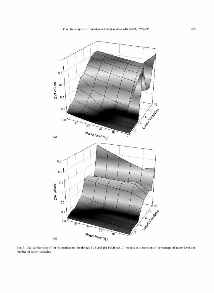
4.1.2.2. Comparison between unsmoothed andsmoothed (second degree seven-point polynomial).The aim of this section is to compare the DW valuesas a function of the percentage of noise added andnumber of latent variables, for the classical PLS andPoLiSh(2, 7) regression models, in order to have amore complete understanding of the variation thatoccur when smoothing.

Fig. 3a and b, present the DW surface plots of theB coefficients for the PLS and PoLiSh(2, 7) models,respectively.

In Fig. 3a (PLS models) the DW values show thedimensionality of the dataset and how the noise affectsthe B coefficient vectors. One can see that between 0and 20% of noise level, the DW values show clearlya distinction between “structured” and “unstructured”latent variables. Above 30% of noise level, this dis-tinction is not very clear, especially at the 50% noiselevel. Despite this, it is possible to use this techniqueas an exploratory tool to study the structure of the re-gression vectors.

When one compares Fig. 3a with Fig. 3b (PoLiShregression models), it is possible to see the influenceof smoothing on the structure of theB coefficients. It isclear in case of Fig. 3b that even at higher noise levels

(40%), one can determine the dimensionality of thedataset and one can also see that, on average, the DWvalues are lower than those in Fig. 3a, due to the morestructuredB coefficient vectors. These results showthat the smoothing approach improves the regressionmodel, giving lower RMSEP values even at high noiselevels (cf. results of Fig. 1).

4.2. Application to real datasets

In this section we will present the application of thistechnique to real datasets, and discuss the advantagesand problems that may arise.

4.2.1. UV–VIS spectra of olive oil — dataset IIThe RMSEP values for the determination of the

degree of acidity of the olive oils are shown inTable 1. The RMSEP values are given for the classi-cal PLS regression (unsmoothed column) and PoLiShregression with several degrees of smoothing. Ascan be seen from the table, six latent variables arenecessary for all models to obtain an acceptable pre-dictive ability. Furthermore, it can be seen that byapplying PoLiSh one has a decrease in the RMSEPvalues from 0.768, for the classical PLS regression

D.N. Rutledge et al. / Analytica Chimica Acta 446 (2001) 281–296 289

Fig. 3. DW surface plot of theB coefficients for the (a) PLS and (b) PoLiSh(2, 7) models as a function of percentage of noise level andnumber of latent variables.

290 D.N. Rutledge et al. / Analytica Chimica Acta 446 (2001) 281–296

Table 1RMSEP values for the determination of the degree of acidity using classical PLS and PoLiSh procedures

LV Unsmoothed PoLiSh(2, 7)

PoLiSh(2, 11)

PoLiSh(2, 15)

PoLiSh(2, 19)

PoLiSh(2, 23)

PoLiSh(2, 27)

PoLiSh(2, 30)

1 4.518 4.519 4.524 4.534 4.548 4.563 4.576 4.5852 2.890 2.891 2.896 2.915 2.954 3.008 3.075 3.1523 1.937 1.935 1.928 1.920 1.913 1.892 1.855 1.8224 1.489 1.489 1.497 1.527 1.589 1.644 1.664 1.6545 0.860 0.861 0.830 0.806 0.815 0.865 0.932 0.9926 0.768 0.728 0.665 0.576 0.504 0.475a 0.486 0.5167 0.848 0.824 0.737 0.649 0.607 0.613 0.618 0.5798 1.076 1.050 1.057 1.003 0.923 0.870 0.802 0.7589 0.967 0.954 0.994 1.069 1.117 1.053 0.949 0.811

10 0.955 0.932 0.917 0.998 1.109 1.270 1.249 0.964

a Minimum RMSEP value.

to 0.475 for the PoLiSh(2, 23) model. An interest-ing result to note is that by using this procedure thedifference between the more important (first six) andthe less important latent variables is higher using thePoLiSh(2, 23) model. For instance, the differencebetween the seventh and the sixth latent variable inthe classical PLS model is 0.080, while this differ-ence increases to 0.138 when using PoLiSh(2, 23).

Fig. 4. B coefficients plots for the determination of the degree of acidity from the UV–VIS spectra, using classical PLS regression andPoLiSh(2, 23).

These results show that one can obtain more robustregression models using PoLiSh and that this proce-dure can also be used as a tool to choose the num-ber of latent variables that characterise a regressionmodel.

In Fig. 4 theB coefficient vectors obtained fromthe classical PLS regression and the PoLiSh(2, 23)models are plotted. It can be seen that small changes

D.N. Rutledge et al. / Analytica Chimica Acta 446 (2001) 281–296 291

Fig. 5. Plot of the rotation angle between classical PLS and PoLiShw-loadings and the DW values for the classical PLSw-loadings.

occurs in theB coefficient profiles. The noisy regionaround 220 nm is slightly smoothed and some shiftsare present in some wavelengths. These shifts seemsto be related to the fact that 23 points are used inthe smoothing step, since it is most noticeable forthe sharp bands. The difference between these twoBcoefficient profiles can be measured in an objectivemeans by calculating the angle between them [12] (cf.Eq. (5)), in this case the angle of rotation was 25.6◦.To have a better insight into the perturbation of thew-loadings with PoLiSh, one can examine both the ro-

Table 2RMSEP values for the determination of fructose content by TD-NMR using classical PLS and PoLiSh procedures

LV Unsmoothed PoLiSh(2, 7)

PoLiSh(2, 11)

PoLiSh(2, 15)

PoLiSh(2, 19)

PoLiSh(2, 23)

PoLiSh(2, 27)

PoLiSh(2, 31)

PoLiSh(2, 35)

1 37.365 37.372 37.360 37.362 37.360 37.352 37.348 37.338 37.3322 14.343 14.349 14.349 14.331 14.330 14.319 14.311 14.309 14.3093 3.853 3.847 3.834 3.840 3.845 3.842 3.857 3.868 3.8874 3.004 3.072 3.020 2.969 2.975 2.933 2.954 2.931a 2.9475 3.605 3.974 4.200 3.872 3.750 3.831 3.745 3.718 3.7396 4.005 5.323 5.588 4.918 4.813 4.605 4.708 4.703 4.6657 3.513 5.106 6.182 5.105 5.308 4.731 4.734 4.551 4.4658 3.311 4.523 6.586 4.733 4.796 3.973 4.128 4.173 4.2739 3.276 4.488 6.586 4.956 5.464 4.365 4.354 5.145 4.357

10 3.344 4.545 7.320 4.623 5.583 4.256 4.030 5.197 5.228

a Minimum RMSEP value.

tation angles of these vectors going from 1 to 10 latentvariables, and the DW profile of the unsmoothedw-loadings.

The rotation angles observed in Fig. 5 shows thatsignificant differences between thew-loadings of theclassical PLS and of PoLiSh(2, 23) models occurs. Atthe same time, and confirming the results shown inTable 2, the DW values of thew-loadings shows thatafter the sixth latent variable the DW value increasessignificantly, showing that latent variables 7–10 con-tain noise.

292 D.N. Rutledge et al. / Analytica Chimica Acta 446 (2001) 281–296

Fig. 6.B coefficients plots for the determination of fructose concentration of aqueous solutions by TD-NMR, using classical PLS regressionand PoLiSh(2, 31).

4.2.2. TD-NMR dataset for the quantification offructose content — dataset III

Table 2 shows the RMSEP values for the determi-nation of fructose concentration of aqueous solutionsby TD-NMR. In this table, one can see that all testedmodels required four latent variables to obtain anacceptable predictive ability. The results shows thatRMSEP slightly decreases for some PoLiSh models,compared to the classical PLS regression procedure(unsmoothed). It can be seen that the minimum RM-SEP value (2.931) obtained was for the PoLiSh(2,31) model, and a similar value (2.933) is obtained forthe PoLiSh(2, 23) model. A characteristic of theseresults (already observed in the previous dataset) canbe seen by comparing the differences between theRMSEP values of the most and less important la-tent variables. A simple calculation shows that themajor differences are observed when one uses thePoLiSh procedure (differences higher than 26%), be-ing maximum with PoLiSh(2, 11) with a differencearound 39%. Therefore, these results shows that thisprocedure can help in choosing the number of latentvariables.

The “optimal” B coefficient vector, correspondingto PoLiSh(2, 31), is plotted in Fig. 6, along theBcoefficient profile of the classical PLS regression. Ascan be seen, the beginning of the curves (region as-sociated with fast relaxation) are very similar for thetwo procedures. It can be seen that PoLiSh(2, 31) hasmuch reduced the noise for the rest of the curve (slowrelaxation). For a better understanding of the noisereduction, the rotation angles between the PLS andPoLiShw-loadings was calculated. These rotation an-gles were: 0.4◦ for LV1, 2.4◦ for LV2, 6.5◦ for LV3,13.5◦ for LV4, 40.4◦ for LV5 and 48.1◦ for LV6. Thesevalues shows that small differences exists between thetwo procedures for the most important latent variables(first four) and that a large difference is observed be-tween the fourth and the fifth latent variables, showingthat the model then starts to include noise.

4.2.3. Determination of the iodine number by FT-IR— dataset IV

Table 3 presents the RMSEP values for the determi-nation of iodine number by FT-IR using the classicalPLS and the PoLiSh procedures. As can be seen in

D.N. Rutledge et al. / Analytica Chimica Acta 446 (2001) 281–296 293

Table 3RMSEP values for the determination of iodine number by FT-IR using classical PLS regression and PoLiSh

LV Unsmoothed PoLiSh(2, 7)

PoLiSh(2, 11)

PoLiSh(2, 15)

PoLiSh(2, 19)

PoLiSh(2, 23)

PoLiSh(2, 27)

PoLiSh(2, 31)

1 46.86 46.85 46.86 46.90 46.95 47.02 47.11 47.202 30.95 30.84 30.89 31.09 31.43 31.90 32.42 32.933 21.02 20.90 20.82 20.73 20.62 20.57 20.58 20.644 19.62 19.41 19.34 19.28 19.22a 19.24 19.31 19.445 19.37 19.34 19.34 19.32 19.29 19.31 19.35 19.436 19.80 19.68 19.66 19.63 19.63 19.68 19.78 19.967 21.51 22.48 22.45 22.30 22.13 21.91 21.69 21.548 22.36 23.14 22.52 22.40 22.32 22.68 22.70 23.269 23.51 23.99 23.77 23.70 23.66 23.77 24.10 24.37

10 23.44 24.15 24.04 23.91 23.81 23.90 24.00 24.02

a Minimum RMSEP value.

this table, the “optimal” model was obtained using afive-latent variable model for the classical PLS regres-sion case. An interesting result is obtained when thePoLiSh procedure is applied. In fact, for all the models,except PoLiSh(2, 31), the RMSEP is lower comparedto the classical PLS. Despite the fact that the “optimal”classical PLS model (RMSEP= 19.37) is not muchgreater than the “optimal” PoLiSh model (RMSEP=

Fig. 7.B coefficients plots for the determination of iodine number based on FT-IR spectra, using classical PLS regression and PoLiSh(2, 19).

19.22), one can see that most of the PoLiSh modelare simpler, i.e. using a lower-dimension regressionmodel (four latent variables). This result seems to in-dicate that the low complexity of these PoLiSh mod-els is related to more robust regression models. Thesesimplified PoLiSh models also seem to indicate thatthere is “noise” in the original dataset that could in-terfere in the construction of the regression model.

294 D.N. Rutledge et al. / Analytica Chimica Acta 446 (2001) 281–296

Fig. 7 shows the twoB coefficient profiles obtainedwith the classical PLS regression and with PoLiSh(2,19). The comparison of these two profiles shows thatsome differences do exist, mainly in the region be-tween 1820 and 600 cm−1. In fact, theB coefficientprofile from the classical PLS regression model showsthe presence of noise which may be due to over-fittingwith the use of five latent variables, instead of the fourlatent variables used by the PoLiSh approach. Hence,it seems that by removing some noise on the low la-tent variables the PoLiSh regression model has be-come more robust. As seen in the previous sections,another way to look at the differences between thetwo present models is by examining the rotation an-gles between the smoothed and unsmoothed models.For theB coefficient profiles shown in Fig. 5, a rota-tion of 25.5◦ was observed, corresponding to a majorchange in the orientation of the PoLiShB coefficientvector. The rotation angles of both the loadingsp andw are plotted in Fig. 8.

As can be seen in Fig. 8, a major change in therotation angle of thew-loadings is observed between

Fig. 8. Rotation angles ofp andw between the classical PLS regression and the PoLiSh(2, 19) model for dataset IV.

the latent variables 4 (17.4◦) and 5 (37.7◦), decreas-ing afterward until the seventh latent variable. Thissame profile is observed on thep vectors. This plotindicates an optimal dimensionality of the regressionmodel of four latent variables for the PoLiSh proce-dure. Looking more closely to the rotation profile ofthe w-loadings, one can observe that there is initiallya slight difference between thew-loadings of PLSand PoLiSh in the first four latent variables, proba-bly meaning that the information extracted by the twoprocedures is similar. After the fourth latent variable(optimal dimensionality), one notes a huge differencebetween the two models, probably due to the noisethat was displaced from the lower latent variables.

The results for this dataset are particularly inter-esting as they show the advantage of using PoLiShto determine the dimensionality of regression models.In fact, as we have seen the cross-validation appliedto the classical PLS gave five latent variables as the“optimal” prediction model (Table 3). However, wehave also seen that PoLiSh has reduced the model di-mensionality to four smoothed latent variables. In fact,

D.N. Rutledge et al. / Analytica Chimica Acta 446 (2001) 281–296 295

Fig. 9. DW profiles of thew andp vectors of the PLS regression on dataset IV.

it seems that the classical PLS prediction model forthis dataset is over-fitted. This is in agreement with thestructure of thew-loadings (orp) of the classical PLSfor this dataset, i.e. by examining the DW profiles, itis clear that in fact the model seems to have only fourlatent variables as shown by PoLiSh. The DW pro-files of p andw obtained from the classical PLS re-gression are plotted in Fig. 9. As can be clearly seen,both profiles show that after the fourth latent variablethere seems to be no useful information present forthe determination of the iodine number. In fact, thelarge change in DW observed between the fourth andthe fifth latent variables suggests a decrease in the sig-nal/noise in the fifth latent variable, i.e. a decrease inthe structure of the “signals” (p andw). We thereforehave several “fast” means of testing the dimensional-ity of a regression model and hence its robustness.

5. Conclusions

The results obtained in this study suggest that theproposed procedure can improve the robustness of PLSregression models and can be a useful tool for the

selection of the number of latent variables. From thesimulated dataset one has seen that this technique canbe most useful in cases were the signals have noiselevels higher than 10–20% of noise. For low noiselevels cases, as the ones shown for the real datasets,this procedure has shown that it is possible to obtainmore robust models compared to the classical PLSregression.

From the obtained results, the smoothing of thew-loadings, in each latent variable, allow the NI-PALS procedure to search for new directions in theN-dimensional space, and as a consequence one canobtain regression models with better predictive abil-ity, since the RMSEP values are lower. It was clearfrom this study that PoLiSh uses new directions inthe latent variables space, since the rotation anglesobserved between, for instance, the PLS and PoLiShw-loadings, are in the most cases significantly high.Hence, it is clear that the presence of noise in thelower latent variables introduce uncertainties that arereduced by the PoLiSh procedure, so more importantinformation is extracted in the low latent variablesgiving parsimonious models. The noise removed fromthe most important latent variables is progressively

296 D.N. Rutledge et al. / Analytica Chimica Acta 446 (2001) 281–296

“displaced” to high latent variables. This can helpin choosing the number of latent variables that themodel should have, since the difference in noiselevels between important and less important latentvariables is very high. The PoLiSh calibration modelsare more robust since the eliminated noise no longercontributes to the definition of the space spanned bythe regression vectors, giving more stable models.

The proposed method, PoLiSh, seems to enhancethe signal to noise ratio and should perform quite wellin cases were the application of PLS could be problem-atic, in terms of choosing the “optimal” dimensional-ity and in terms of calibration robustness. The anal-ysis of some characteristics of PoLiSh and PLS vec-tors, such as smoothing degrees, RMSEP behaviour,and DW profiles (forp, w andb vectors), may providemore objectively methodologies to build more robustregression models.

Despite the obtained results, several studies shouldbe addressed for the full characterisation of PoLiSh.Among these, the properties of the polynomials usedin the smoothing step should be better understood andthe behaviour of the displaced noise should be ad-dressed, i.e. how it propagates throughout the higherlatent variables.

Acknowledgements

A. Barros thanks FCT (Portugal) for the Post-Doctoral Grant no. PRAXIS XXI/BPD/18824/99.

References

[1] D.N. Rutledge, A.S. Barros, M.C. Vackier, S. Baumberger, C.Lapierre, Analysis of time domain NMR and other signals,in: P.S. Belton, B.P. Hills, G.A. Webb (Eds.), Advancesin Magnetic Resonance in Food Science, Royal Society ofChemistry, London, 1999, pp. 203–216.

[2] D.N. Rutledge, A.S. Barros, F. Gaudard, ANOVA and factoranalysis applied to time domain NMR signals, Magn. Reson.Chem. 35 (1997) S13–S21.

[3] D.N. Rutledge, A.S. Barros, A method for detectinginformation in signals: application to 2D time domain-NMRdata, The Analyst 123 (1998) 551–559.

[4] A.S. Barros, D.N. Rutledge, Genetic algorithm applied to theselection of principal components, Chemom. Intell. Lab. Syst.40 (1) (1998) 65–81.

[5] A.G. Marshall, F.R. Verdun, Fourier Transforms in NMR,Optical, and Mass Spectrometry: A User’s Handbook,Elsevier, Amsterdam, 1990.

[6] R. Tomassone, C. Dervin, J.P. Masson, Biométrie:modélisation de phénomènes biologiques, Masson, Paris,1993, p. 409.

[7] A. Savitsky, M.J.E. Golay, Smoothing and differentiation ofdata by simplified least-squares procedures, Anal. Chem. 36(1964) 1627–1639.

[8] J. Steiner, Y. Termonia, J. Deltour, Comments on smoothingand differentiation of data by simplified least-squaresprocedures, Anal. Chem. 44 (1972) 1906–1909.

[9] P.A. Gorry, General least-squares smoothing and differen-tiation by convolution (Savitsky–Golay) method, Anal. Chem.62 (1990) 570–573.

[10] J. Durbin, G.S. Watson, Testing for serial correlations inleast-squares regression, Biometrika 37 (1950) 409–428.

[11] P. Geladi, B. Kowalski, Partial least-squares regression: atutorial, Anal. Chim. Acta 198 (1986) 1–17.

[12] K.V. Mardia, J.T. Kent, J.M. Bibby, Multivariate Analysis,Academic Press, London, 1994, p. 482.