ARTICLE IN PRESS

0167-7152/$ - se

doi:10.1016/j.sp

�CorrespondE-mail addr

Statistics & Probability Letters 76 (2006) 1265–1272

www.elsevier.com/locate/stapro

On equality and proportionality of ordinary least squares,weighted least squares and best linear unbiased estimators in the

general linear model

Yongge Tiana, Douglas P. Wiensb,�

aSchool of Economics, Shanghai University of Finance and Economics, Shanghai 200433, ChinabDepartment of Mathematical and Statistical Sciences, University of Alberta, Edmonton, Alta, Canada T6G 2G1

Received 4 November 2004; received in revised form 23 December 2005

Available online 20 February 2006

Abstract

Equality and proportionality of the ordinary least-squares estimator (OLSE), the weighted least-squares estimator

(WLSE), and the best linear unbiased estimator (BLUE) for Xb in the general linear (Gauss–Markov) model M ¼

fy;Xb; s2Rg are investigated through the matrix rank method.

r 2006 Elsevier B.V. All rights reserved.

MSC: Primary 62J05; 62H12; 15A24

Keywords: General linear model; Equality; Proportionality; OLSE; WLSE; BLUE; Projectors; Rank formulas for partitioned matrices

1. Introduction

Consider the general linear (Gauss–Markov) model

M ¼ fy;Xb;Rg, (1)

where X is a nonnull n� p known matrix, y is an n� 1 observable random vector with expectation EðyÞ ¼ Xb

and with the covariance matrix CovðyÞ ¼ R, b is a p� 1 vector of unknown parameters, and R is an n� n

symmetric nonnegative definite (n.n.d.) matrix, known entirely except for a positive constant multiplier. In thispaper, we investigate some special relations among the ordinary least-squares estimator (OLSE), the weightedleast-squares estimator (WLSE), and the best linear unbiased estimator (BLUE) for Xb in the model M.

Throughout this paper, A0, rðAÞ and RðAÞ represent the transpose, the rank and the range (column space) ofa real matrix A, respectively; Ay denotes the Moore–Penrose inverse of A with the properties AAyA ¼ A,AyAAy ¼ Ay, ðAAyÞ0 ¼ AAy and ðAyAÞ0 ¼ AyA. In addition, let PA ¼ AAy and QA ¼ I� PA.

Let M be as given in (1). The OLSE bb of b is defined to be a vector minimizing ky� Xbk2 ¼

ðy� XbÞ0ðy� XbÞ and OLSEðXbÞ is defined to be Xbb. Suppose V is an n� n n.n.d. matrix. The WLSE eb of b is

e front matter r 2006 Elsevier B.V. All rights reserved.

l.2006.01.005

ing author. Tel.: +1780 4924406; fax: +1 780 4926826.

esses: yongge@mail.shufe.edu.cn (Y. Tian), doug.wiens@ualberta.ca (D.P. Wiens).

ARTICLE IN PRESSY. Tian, D.P. Wiens / Statistics & Probability Letters 76 (2006) 1265–12721266

defined to be a vector b minimizing ky� Xbk2V ¼ ðy� XbÞ0Vðy� XbÞ, and WLSEVðXbÞ is defined to be Xeb.When V ¼ In, WLSEIn

ðXbÞ ¼ OLSEðXbÞ. The weight matrix V in WLSEVðXbÞ can be constructed from thegiven matrix X and R, for example, V ¼ Ry or V ¼ ðXTX0 þ RÞy, see, e.g., Rao (1971). The BLUE of Xb is alinear estimator Gy such that EðGyÞ ¼ Xb and for any other linear unbiased estimator My of Xb, CovðMyÞ �

CovðGyÞ ¼MRM0 �GRG0 is nonnegative definite. The three estimators are well known and have beenextensively investigated in the literature.

Definition 1. Let X be an n� p matrix, and let V and R be two n� n symmetric n.n.d. matrices.

(a)

The projector into the range of X under the seminorm kxk2V ¼ x0Vx is defined to be

PX:V ¼ XðX0VXÞyX0Vþ ½X� XðVXÞyðVXÞ�U, (2)

where U is arbitrary.

(b) The BLUE projector PXkR is defined to be the solution G satisfying the equation

G½X;RQX� ¼ ½X; 0�,

which can be expressed as

PXkR ¼ ½X; 0�½X;RQX�y þU1ðIn � ½X;RQX�½X;RQX�

yÞ,

where U1 is arbitrary. The product PXkRR is unique and can be written as

PXkRR ¼ PXR� PXRðQXRQXÞyR. (3)

The following results on the OLSE, WLSE and BLUE of Xb in M are well known, see, e.g., Mitra and Rao(1974) and Puntanen and Styan (1989).

Lemma 1. Let M be as given in (1). Then:

(a)

The OLSE of Xb in M is unique, and can be written as OLSEðXbÞ ¼ PXy. In this case,

E½OLSEðXbÞ� ¼ Xb and Cov½OLSEðXbÞ� ¼ PXRPX.

(b)

The general expression of the WLSE of Xb in M can be written as WLSEVðXbÞ ¼ PX:Vy. In this case,

E½WLSEVðXbÞ� ¼ PX:VXb and Cov½WLSEVðXbÞ� ¼ PX:VRP0X:V.

In particular, WLSEVðXbÞ is unique if and only if rðVXÞ ¼ rðXÞ. In such a case, PX:VX ¼ X and WLSEVðXbÞ

is unbiased.

(c) The general expression of the BLUE of Xb in M can be written as BLUEðXbÞ ¼ PXkRy. In this case,

E½BLUEðXbÞ� ¼ Xb and Cov½BLUEðXbÞ� ¼ PXkRRP0XkR.

Moreover, Cov½BLUEðXbÞ� can be expressed as

Cov½BLUEðXbÞ� ¼ PXRPX � PXRðQXRQXÞyRPX.

In particular, BLUEðXbÞ is unique if y 2 R½X;R�, the range of ½X;R�.

Various properties of PX:V and PXkR can be found in Mitra and Rao (1974), and Puntanen and Styan (1989).Because these estimators are derived from different optimal criteria, they are not necessarily equal. Aninteresting problem on these estimators is to give necessary and sufficient conditions for them to be equal. Ifthis is true, one can use the OLSE of Xb instead of the BLUE of Xb. Further, it is of interest to consider theproportionality of these estimators.

In order to compare two estimators for an unknown parameter vector, various efficiency functions havebeen introduced. The most frequently used measure for relations between two unbiased estimators L1y and

ARTICLE IN PRESSY. Tian, D.P. Wiens / Statistics & Probability Letters 76 (2006) 1265–1272 1267

L2y of b with both CovðL1yÞ and CovðL2yÞ nonsingular is the D-relative efficiency

effDðL1y;L2yÞ ¼det½CovðL2yÞ�

det½CovðL2yÞ�.

A similar relative efficiency function is also defined for the determinants of the information matricescorresponding to two designs for a linear regression model. Other relative efficiency functions can be definedthrough the traces and norms of covariance matrices, for example,

effAðL1y;L2yÞ ¼tr½CovðL1yÞ�

tr½CovðL2yÞ�.

If effDðL1y;L2yÞ ¼ 1, i.e., det½CovðL1yÞ� ¼ det½CovðL2yÞ�, the two estimators L1y and L2y are said to have the

same D-efficiency, and is denoted by L1y�DL2y.

In addition to the determinant equality det½CovðL1yÞ� ¼ det½CovðL2yÞ�, some strong relations between twounbiased estimators are defined as follows.

Definition 2. Suppose that L1y and L2y are two unbiased linear estimators of b in (1).

(a)

The two estimators are said to have the same efficiency if

CovðL1yÞ ¼ CovðL2yÞ, (4)

and this is denoted by L1y�CL2y.

(b)

The two estimators are said to be identical (coincide) with probability 1 if

CovðL1y� L2yÞ ¼ 0, (5)

and this is denoted by L1y�PL2y.

Clearly (4) is equivalent to

L1RL01 ¼ L2RL

02, (6)

and (5) is equivalent to ðL1 � L2ÞRðL1 � L2Þ0¼ 0, i.e.,

L1R ¼ L2R. (7)

It is easy to see from (6) and (7) that

L1y�PL2y) L1y�

CL2y) L1y�

DL2y.

However, the reverse implication is not true. For example, let

R ¼2 1

1 2

� �; L1 ¼ ½1;�1�; L2 ¼ ½�1; 1�.

Then

L1RL01 ¼ L2RL

02 ¼ 2; but ðL1 � L2ÞR ¼ ½2;�2�a0.

Many authors investigated the equalities among these estimators using Definition 2(a); see, e.g., Baksalaryand Puntanen (1989), Puntanen and Styan (1989), Young et al. (2000), and GroX et al. (2001) among others. Inthis paper, we use Definition 2(b) to characterize the relations between two estimators.

Lemma 2. Let M be as given in (1), and suppose L1y and L2y are two linear estimators for Xb in M. Then

L1y ¼ L2y with probability 1, i.e., L1y�PL2y, if and only if L1X ¼ L2X and L1R ¼ L2R, i.e.,

L1½X;R� ¼ L2½X;R�.

The rank of a matrix is defined to be the dimension of the column space or row space of the matrix. It hasbeen recognized since the 1970s that rank equalities for matrices provide a powerful method for findinggeneral properties of matrix expressions. In fact, for any two matrices A and B of the same size, the equality

ARTICLE IN PRESSY. Tian, D.P. Wiens / Statistics & Probability Letters 76 (2006) 1265–12721268

A ¼ B holds if and only if rðA� BÞ ¼ 0; two sets S1 and S2 consisting of matrices of the same size have acommon matrix if and only if minA2S1;B2S2

rðA� BÞ ¼ 0; the set inclusion S1 � S2 holds if and only ifmaxA2S1

minB2S2rðA� BÞ ¼ 0. If some formulas for the rank of A� B are derived, they can be used to

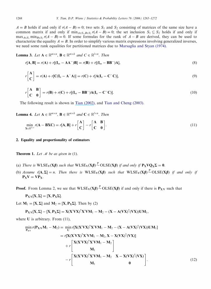
characterize the equality A ¼ B. In order to simplify various matrix expressions involving generalized inverses,we need some rank equalities for partitioned matrices due to Marsaglia and Styan (1974).

Lemma 3. Let A 2 Rm�n, B 2 Rm�k and C 2 Rl�n. Then

r½A;B� ¼ rðAÞ þ r½ðIm � AA�ÞB� ¼ rðBÞ þ r½ðIm � BB�ÞA�, (8)

rA

C

� �¼ rðAÞ þ r½CðIn � A�AÞ� ¼ rðCÞ þ r½AðIn � C�CÞ�, (9)

rA B

C 0

� �¼ rðBÞ þ rðCÞ þ r½ðIm � BB�ÞAðIn � C�CÞ�. (10)

The following result is shown in Tian (2002), and Tian and Cheng (2003).

Lemma 4. Let A 2 Rm�n, B 2 Rm�k and C 2 Rl�n. Then

minX2Rk�l

rðA� BXCÞ ¼ r½A;B� þ rA

C

� �� r

A B

C 0

� �. (11)

2. Equality and proportionality of estimators

Theorem 1. Let M be as given in (1).

(a)

There is WLSEVðXbÞ such that WLSEVðXbÞ �POLSEðXbÞ if and only if PXVQXR ¼ 0.

(b)

Assume r½A;R� ¼ n. Then there is WLSEVðXbÞ such that WLSEVðXbÞ �POLSEðXbÞ if and only if

PXV ¼ VPX.

Proof. From Lemma 2, we see that WLSEVðXbÞ �POLSEðXbÞ if and only if there is PX:V such that

PX:V½X;R� ¼ ½X;PXR�.

Let M1 ¼ ½X;R� and M2 ¼ ½X;PXR�. Then by (2)

PX:V½X;R� � ½X;PXR� ¼ XðX0VXÞyX0VM1 �M2 � ðX� AðVXÞyðVXÞÞUM1,

where U is arbitrary. From (11),

minPX:V

rðPX:VM1 �M2Þ ¼ minU

r½XðX0VXÞyX0VM1 �M2 � ðX� AðVXÞyðVXÞÞUM1�

¼ r½XðX0VXÞyX0VM1 �M2;X� XðVXÞyðVXÞ�

þ rXðX0VXÞyX0VM1 �M2

M1

" #

� rXðX0VXÞyX0VM1 �M2 X� XðVXÞyðVXÞ

M1 0

" #. ð12Þ

ARTICLE IN PRESSY. Tian, D.P. Wiens / Statistics & Probability Letters 76 (2006) 1265–1272 1269

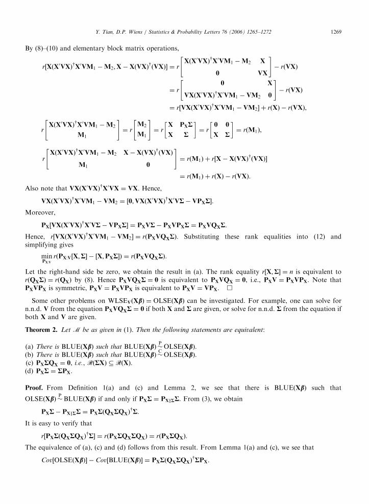
By (8)–(10) and elementary block matrix operations,

r½XðX0VXÞyX0VM1 �M2;X� XðVXÞyðVXÞ� ¼ rXðX0VXÞyX0VM1 �M2 X

0 VX

" #� rðVXÞ

¼ r0 X

VXðX0VXÞyX0VM1 � VM2 0

" #� rðVXÞ

¼ r½VXðX0VXÞyX0VM1 � VM2� þ rðXÞ � rðVXÞ,

rXðX0VXÞyX0VM1 �M2

M1

" #¼ r

M2

M1

" #¼ r

X PXR

X R

� �¼ r

0 0

X R

� �¼ rðM1Þ,

rXðX0VXÞyX0VM1 �M2 X� XðVXÞyðVXÞ

M1 0

" #¼ rðM1Þ þ r½X� XðVXÞyðVXÞ�

¼ rðM1Þ þ rðXÞ � rðVXÞ.

Also note that VXðX0VXÞyX0VX ¼ VX. Hence,

VXðX0VXÞyX0VM1 � VM2 ¼ ½0;VXðX0VXÞyX0VR� VPXR�.

Moreover,

PX½VXðX0VXÞyX0VR� VPXR� ¼ PXVR� PXVPXR ¼ PXVQXR.

Hence, r½VXðX0VXÞyX0VM1 � VM2� ¼ rðPXVQXRÞ. Substituting these rank equalities into (12) andsimplifying gives

minPX:V

rðPX:V½X;R� � ½X;PXR�Þ ¼ rðPXVQXRÞ.

Let the right-hand side be zero, we obtain the result in (a). The rank equality r½X;R� ¼ n is equivalent torðQXRÞ ¼ rðQXÞ by (8). Hence PXVQXR ¼ 0 is equivalent to PXVQX ¼ 0, i.e., PXV ¼ PXVPX. Note thatPXVPX is symmetric, PXV ¼ PXVPX is equivalent to PXV ¼ VPX. &

Some other problems on WLSEVðXbÞ ¼ OLSEðXbÞ can be investigated. For example, one can solve forn.n.d. V from the equation PXVQXR ¼ 0 if both X and R are given, or solve for n.n.d. R from the equation ifboth X and V are given.

Theorem 2. Let M be as given in (1). Then the following statements are equivalent:

(a)

There is BLUEðXbÞ such that BLUEðXbÞ �POLSEðXbÞ.

(b)

There is BLUEðXbÞ such that BLUEðXbÞ �COLSEðXbÞ.

(c)

PXRQX ¼ 0, i.e., RðRXÞ � RðXÞ. (d) PXR ¼ RPX.

Proof. From Definition 1(a) and (c) and Lemma 2, we see that there is BLUEðXbÞ such that

OLSEðXbÞ �PBLUEðXbÞ if and only if PXR ¼ PXkRR. From (3), we obtain

PXR� PXkRR ¼ PXRðQXRQXÞyR.

It is easy to verify that

r½PXRðQXRQXÞyR� ¼ rðPXRQXRQXÞ ¼ rðPXRQXÞ.

The equivalence of (a), (c) and (d) follows from this result. From Lemma 1(a) and (c), we see that

Cov½OLSEðXbÞ� � Cov½BLUEðXbÞ� ¼ PXRðQXRQXÞyRPX.

ARTICLE IN PRESSY. Tian, D.P. Wiens / Statistics & Probability Letters 76 (2006) 1265–12721270

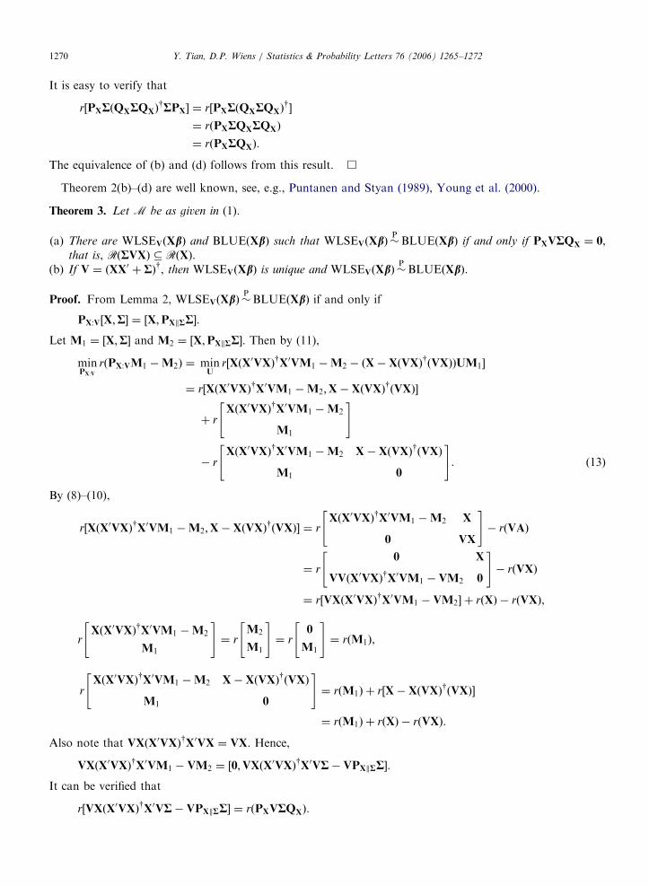
It is easy to verify that

r½PXRðQXRQXÞyRPX� ¼ r½PXRðQXRQXÞ

y�

¼ rðPXRQXRQXÞ

¼ rðPXRQXÞ.

The equivalence of (b) and (d) follows from this result. &

Theorem 2(b)–(d) are well known, see, e.g., Puntanen and Styan (1989), Young et al. (2000).

Theorem 3. Let M be as given in (1).

(a)

There are WLSEVðXbÞ and BLUEðXbÞ such that WLSEVðXbÞ �PBLUEðXbÞ if and only if PXVRQX ¼ 0,

that is, RðRVXÞ � RðXÞ.

(b) If V ¼ ðXX0 þ RÞy, then WLSEVðXbÞ is unique and WLSEVðXbÞ �

PBLUEðXbÞ.

Proof. From Lemma 2, WLSEVðXbÞ �PBLUEðXbÞ if and only if

PX:V½X;R� ¼ ½X;PXkRR�.

Let M1 ¼ ½X;R� and M2 ¼ ½X;PXkRR�. Then by (11),

minPX:V

rðPX:VM1 �M2Þ ¼ minU

r½XðX0VXÞyX0VM1 �M2 � ðX� XðVXÞyðVXÞÞUM1�

¼ r½XðX0VXÞyX0VM1 �M2;X� XðVXÞyðVXÞ�

þ rXðX0VXÞyX0VM1 �M2

M1

" #

� rXðX0VXÞyX0VM1 �M2 X� XðVXÞyðVXÞ

M1 0

" #. ð13Þ

By (8)–(10),

r½XðX0VXÞyX0VM1 �M2;X� XðVXÞyðVXÞ� ¼ rXðX0VXÞyX0VM1 �M2 X

0 VX

" #� rðVAÞ

¼ r0 X

VVðX0VXÞyX0VM1 � VM2 0

" #� rðVXÞ

¼ r½VXðX0VXÞyX0VM1 � VM2� þ rðXÞ � rðVXÞ,

rXðX0VXÞyX0VM1 �M2

M1

" #¼ r

M2

M1

" #¼ r

0

M1

" #¼ rðM1Þ,

rXðX0VXÞyX0VM1 �M2 X� XðVXÞyðVXÞ

M1 0

" #¼ rðM1Þ þ r½X� XðVXÞyðVXÞ�

¼ rðM1Þ þ rðXÞ � rðVXÞ.

Also note that VXðX0VXÞyX0VX ¼ VX. Hence,

VXðX0VXÞyX0VM1 � VM2 ¼ ½0;VXðX0VXÞyX0VR� VPXkRR�.

It can be verified that

r½VXðX0VXÞyX0VR� VPXkRR� ¼ rðPXVRQXÞ.

ARTICLE IN PRESSY. Tian, D.P. Wiens / Statistics & Probability Letters 76 (2006) 1265–1272 1271

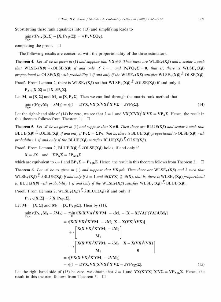
Substituting these rank equalities into (13) and simplifying leads to

minPX:V

rðPX:V½X;R� � ½X;PXkRR�Þ ¼ rðPXVRQXÞ,

completing the proof. &

The following results are concerned with the proportionality of the three estimators.

Theorem 4. Let M be as given in (1) and suppose that VXa0. Then there are WLSEVðXbÞ and a scalar l such

that WLSEVðXbÞ �PlOLSEðXbÞ if and only if l ¼ 1 and PXVQXR ¼ 0, that is, there is WLSEVðXbÞ

proportional to OLSEðXbÞ with probability 1 if and only if the WLSEVðXbÞ satisfies WLSEVðXbÞ �POLSEðXbÞ.

Proof. From Lemma 2, there is WLSEVðXbÞ so that WLSEVðXbÞ �PlOLSEðXbÞ if and only if

PX:V½X;R� ¼ ½lX; lPXR�.

Let M1 ¼ ½X;R� and M2 ¼ ½X;PXR�. Then we can find through the matrix rank method that

minPX:V

rðPX:VM1 � lM2Þ ¼ r½ð1� lÞVX;VXðX0VXÞyX0VR� lVPXR�. (14)

Let the right-hand side of (14) be zero, we see that l ¼ 1 and VXðX0VXÞyX0VR ¼ VPXR. Hence, the result inthis theorem follows from Theorem 1. &

Theorem 5. Let M be as given in (1) and suppose that Xa0. Then there are BLUEðXbÞ and scalar l such that

BLUEðXbÞ �PlOLSEðXbÞ if and only if PXR ¼ RPX, that is, there is BLUEðXbÞ proportional to OLSEðXbÞ with

probability 1 if and only if the BLUEðXbÞ satisfies BLUEðXbÞ �POLSEðXbÞ.

Proof. From Lemma 2, BLUEðXbÞ �PlOLSEðXbÞ holds, if and only if

X ¼ lX and RPXR ¼ lPXkRR,

which are equivalent to l¼1 and RPXR ¼ PXkRR. Hence, the result in this theorem follows from Theorem 2. &

Theorem 6. Let M be as given in (1) and suppose that VXa0. Then there are WLSEVðXbÞ and l such that

WLSEVðXbÞ �PlBLUEðXbÞ if and only if l ¼ 1 and RðRVXÞ � RðXÞ, that is, there is WLSEVðXbÞ proportional

to BLUEðXbÞ with probability 1 if and only if the WLSEVðXbÞ satisfies WLSEVðXbÞ �PBLUEðXbÞ.

Proof. From Lemma 2, WLSEVðXbÞ �PlBLUEðXbÞ if and only if

PAX:V½X;R� ¼ l½X;PXkRR�.

Let M1 ¼ ½X;R� and M2 ¼ ½X;PXkRR�. Then by (11),

minPX:V

rðPX:VM1 � lM2Þ ¼ minU

r½XðX0VAÞyX0VM1 � lM2 � ðX� XðVAÞyðVAÞÞUM1�

¼ r½XðX0VXÞyX0VM1 � lM2;X� XðVXÞyðVXÞ�

þ rXðX0VXÞyX0VM1 � lM2

M1

" #

� rXðX0VXÞyX0VM1 � lM2 X� XðVXÞyðVXÞ

M1 0

" #¼ r½VXðX0VXÞyX0VM1 � lVM2�

¼ r½ð1� lÞVX;VXðX0VXÞyX0VR� lVPXkRR�. ð15Þ

Let the right-hand side of (15) be zero, we obtain that l ¼ 1 and VXðX0VXÞyX0VR ¼ VPXkRR. Hence, theresult in this theorem follows from Theorem 3. &

ARTICLE IN PRESSY. Tian, D.P. Wiens / Statistics & Probability Letters 76 (2006) 1265–12721272

It can be seen from Theorems 4–6 that if any two of the OLSE, WLSE and BLUE for Xb in the model (1)are proportional with probability 1, the two estimators are identical with probability 1.

Many other problems on the model (1) can be investigated through the matrix rank method. For example,assume that the general linear model fy;Xb;Rg incorrectly specifies the covariance matrix as s2R0, where R0 isa given n.n.d. matrix and s2 is a positive parameter (possibly unknown). Then consider the relations betweenthe BLUEs of Xb in the original model and the misspecified model fy;Xb;s2R0g. Some previous results on therelations between the BLUEs of Xb in the two models can be found in Mitra and Moore (1973), and Mathew(1983). In addition, it is of interest to consider partial coincidence and partial proportionality of the OLSE,WLSE and BLUE of Xb in (1), as well as to consider coincidence and proportionality of the OLSE, WLSEand BLUE of Xb in (1) under a restriction Ab ¼ b.

Acknowledgment

The research of both authors was supported by the Natural Sciences and Engineering Research Council ofCanada.

References

Baksalary, J.K., Puntanen, S., 1989. Weighted-least squares estimation in the general Gauss–Markov model. In: Dodge, Y. (Ed.),

Statistical Data Analysis and Inference. Elsevier, New York, pp. 355–368.

GroX, G., Trenkler, T., Werner, H.J., 2001. The equality of linear transformations of the ordinary least squares estimator and the best

linear unbiased estimator. Sankhya Ser. A 63, 118–127.

Marsaglia, G., Styan, G.P.H., 1974. Equalities and inequalities for ranks of matrices. Linear Multilinear Algebra 2, 269–292.

Mathew, T., 1983. Linear estimation with an incorrect dispersion matrix in linear models with a common linear part. J. Amer. Statist.

Assoc. 78, 468–471.

Mitra, S.K., Moore, B.J., 1973. Gauss-Markov estimation with an incorrect dispersion matrix. Sankhya Ser. A 35, 139–152.

Mitra, S.K., Rao, C.R., 1974. Projections under seminorms and generalized Moore–Penrose inverses. Linear Algebra Appl. 9, 155–167.

Puntanen, S., Styan, G.P.H., 1989. The equality of the ordinary least squares estimator and the best linear unbiased estimator. With

comments by O. Kempthorne, S.R. Searle, and a reply by the authors. Amer. Statist. 43, 153–164.

Rao, C.R., 1971. Unified theory of linear estimation. Sankhya Ser. A 33, 371–394.

Tian, Y., 2002. The maximal and minimal ranks of some expressions of generalized inverses of matrices. Southeast Asian Bull. Math. 25,

745–755.

Tian, Y., Cheng, S., 2003. The maximal and minimal ranks of A� BXC with applications. New York J. Math. 9, 345–362.

Young, D.M., Odell, P.L., Hahn, W., 2000. Nonnegative-definite covariance structures for which the blu, wls, and ls estimators are equal.

Statist. Probab. Lett. 49, 271–276.