Embed Size (px)
Citation preview
University of New MexicoUNM Digital Repository
Mathematics & Statistics ETDs Electronic Theses and Dissertations
2-9-2010
Contributions to partial least squares regressionand supervised principal component analysismodelingYizho Jiang
Follow this and additional works at: https://digitalrepository.unm.edu/math_etds
This Dissertation is brought to you for free and open access by the Electronic Theses and Dissertations at UNM Digital Repository. It has beenaccepted for inclusion in Mathematics & Statistics ETDs by an authorized administrator of UNM Digital Repository. For more information, pleasecontact [email protected].
Recommended CitationJiang, Yizho. "Contributions to partial least squares regression and supervised principal component analysis modeling." (2010).https://digitalrepository.unm.edu/math_etds/72

Yizhou JiangCandidate
Mathematics & StatisticsDepartment
This dissertation is approved, and it is acceptable in qualityand form for publication:
~#fJ"'-'_G_ab_n_·e_I_H_,u_ert_a ~
~ lCS
Contributions to Partial Least SquaresRegression and Supervised Principal
Component Analysis Modeling
by
Yizhou Jiang
B.A., English, Changchun University, China, 1997M.A., Communication, University of New Mexico, 2003
M.S., Statistics, University of New Mexico, 2004
DISSERTATION
Submitted in Partial Fulfillment of the
Requirements for the Degree of
Doctor of Philosophy
Statistics
The University of New Mexico
Albuquerque, New Mexico
December, 2009

c©2009, Yizhou Jiang
iii

Dedication
To my parents and my wife for their support and encouragement.
To my son who gives me the greatest joy of life.
iv

Acknowledgments
I would like to express my deepest gratitude to my adviser, Professor Edward Bedrick.Without his guidance and persistent help this dissertation would not have beenpossible. I will always appreciate his great patience, encouragement and time.
I would also like to thank my committee members, Professor Michele Guindani,Professor Gabriel Huerta, and Professor Huining Kang for their valuable suggestionsand comments.
v
Contributions to Partial Least SquaresRegression and Supervised Principal
Component Analysis Modeling
by
Yizhou Jiang
ABSTRACT OF DISSERTATION
Submitted in Partial Fulfillment of the
Requirements for the Degree of
Doctor of Philosophy
Statistics
The University of New Mexico
Albuquerque, New Mexico
December, 2009
Contributions to Partial Least SquaresRegression and Supervised Principal
Component Analysis Modeling
by
Yizhou Jiang
B.A., English, Changchun University, China, 1997
M.A., Communication, University of New Mexico, 2003
M.S., Statistics, University of New Mexico, 2004
Ph.D., Statistics, University of New Mexico, 2009
Abstract
Latent structure techniques have recently found extensive use in regression analysis
for high dimensional data. This thesis attempts to examine and expand two of such
methods, Partial Least Squares (PLS) regression and Supervised Principal Compo-
nent Analysis (SPCA). We propose several new algorithms, including a quadratic
spline PLS, a cubic spline PLS, two fractional polynomial PLS algorithms and two
multivariate SPCA algorithms. These new algorithms were compared to several pop-
ular PLS algorithms using real and simulated datasets. Cross validation was used to
assess the goodness-of-fit and prediction accuracy of the various models. Strengths
and weaknesses of each method were also discussed based on model stability, robust-
ness and parsimony.
vii

The linear PLS and the multivariate SPCA methods were found to be the most
robust among the methods considered, and usually produced models with good fit
and prediction. Nonlinear PLS methods are generally more powerful in fitting non-
linear data, but they had the tendency to over-fit, especially with small sample sizes.
A forward stepwise predictor pre-screening procedure was proposed for multivariate
SPCA and our examples demonstrated its effectiveness in picking a smaller number
of predictors than the standard univariate testing procedure.
viii
Contents
List of Figures xi
List of Tables xiii
1 Introduction 1
2 Partial Least Squares 3
2.1 Linear PLS: NIPALS and SIMPLS . . . . . . . . . . . . . . . . . . . 5
2.1.1 Iterative PLS algorithm: NIPALS . . . . . . . . . . . . . . . . 7
2.1.2 Non-iterative Linear PLS algorithm: SIMPLS . . . . . . . . . 8
2.2 Nonlinear PLS with polynomial inner
relations . . . . . . . . . . . . . . . . . . . . . . . . . . . . . . . . . . 14
2.2.1 Wold’s Quadratic PLS . . . . . . . . . . . . . . . . . . . . . . 17
2.2.2 Error-based quadratic PLS . . . . . . . . . . . . . . . . . . . . 18
2.2.3 The Box-Tidwell PLS algorithm . . . . . . . . . . . . . . . . . 23
2.2.4 Spline nonlinear PLS algorithms . . . . . . . . . . . . . . . . . 29
ix
Contents
2.3 Simplified Spline and Fractional Polynomial PLS . . . . . . . . . . . 31
2.3.1 Simplified Spline PLS . . . . . . . . . . . . . . . . . . . . . . . 31
2.3.2 Fractional Polynomial PLS . . . . . . . . . . . . . . . . . . . . 32
2.3.3 Example . . . . . . . . . . . . . . . . . . . . . . . . . . . . . . 45
2.4 PLS Prediction and Cross Validation . . . . . . . . . . . . . . . . . . 51
2.4.1 Obtaining PLS Predictions . . . . . . . . . . . . . . . . . . . . 51
2.4.2 Model Selection and Validation with Cross Validation . . . . . 52
3 A Comparison of PLS methods 55
3.1 Real Data . . . . . . . . . . . . . . . . . . . . . . . . . . . . . . . . . 56
3.2 Simulated Non-Linear Data . . . . . . . . . . . . . . . . . . . . . . . 58
3.3 Results . . . . . . . . . . . . . . . . . . . . . . . . . . . . . . . . . . . 59
3.4 Discussion . . . . . . . . . . . . . . . . . . . . . . . . . . . . . . . . . 64
4 Supervised Principal Component Analysis with Multiple Responses 80
4.1 Univariate SPCA . . . . . . . . . . . . . . . . . . . . . . . . . . . . . 81
4.2 Multivariate Extension of SPCA . . . . . . . . . . . . . . . . . . . . . 83
4.3 Examples . . . . . . . . . . . . . . . . . . . . . . . . . . . . . . . . . 85
4.4 Discussion . . . . . . . . . . . . . . . . . . . . . . . . . . . . . . . . . 100
5 Conclusion 101
x

List of Figures
2.1 Plots of possible non-differential or discontinuous inner relation func-
tions for BTPLS. . . . . . . . . . . . . . . . . . . . . . . . . . . . . 28
2.2 Plots of example functions in f1(t) with power 2, 0.5, 1 and -1. . . . 35
2.3 Trace plots for parameter estimates using MFPPLS-II with discrete
powers (Cosmetics Data, the first component). . . . . . . . . . . . . 38
2.4 Trace plots for estimates of t1 using MFPPLS-II with discrete powers
(Cosmetics Data). . . . . . . . . . . . . . . . . . . . . . . . . . . . . 40
2.5 Trace plots for estimates of u1 using MFPPLS-II with discrete powers
(Cosmetics Data). . . . . . . . . . . . . . . . . . . . . . . . . . . . . 41
2.6 Trace plots for parameter estimates using MFPPLS-II with continu-
ous powers (Cosmetics Data, the first component). . . . . . . . . . . 42
2.7 Trace plots for estimates of t1 using MFPPLS-II with continuous
powers (Cosmetics Data). . . . . . . . . . . . . . . . . . . . . . . . . 43
2.8 Trace plots for estimates of u1 using MFPPLS-II with continuous
powers (Cosmetics Data). . . . . . . . . . . . . . . . . . . . . . . . . 44
2.9 Plots of ta vs. ua with the fitted curves, MFPPLS-I. . . . . . . . . . 47
xi

List of Figures
2.10 Plots of ta vs. ua with the fitted curves, MFPPLS-II. . . . . . . . . 48
2.11 Plots of ta vs. ua with the fitted curves, NIPALS. . . . . . . . . . . 49
2.12 Plots of ta vs. ua with the fitted curves, BTPLS . . . . . . . . . . . 50
xii

List of Tables
2.1 Outline of the NIPALS Algorithm . . . . . . . . . . . . . . . . . . . 11
2.2 Basic idea of the SIMPLS Algorithm . . . . . . . . . . . . . . . . . . 12
2.3 Steps for the SIMPLS Algorithm . . . . . . . . . . . . . . . . . . . . 13
2.4 The error-based method for updating X weights w∗a. . . . . . . . . . 21
2.5 Steps in the error-based polynomial PLS algorithms. . . . . . . . . . 22
2.6 Partial derivative matrix Z in MFPPLS-I and MFPPLS-II. . . . . . 39
2.7 MFPPLS-I fits the Cosmetics Data. . . . . . . . . . . . . . . . . . . 46
2.8 MFPPLS-II fits the Cosmetics Data. . . . . . . . . . . . . . . . . . . 46
2.9 NIPALS fits the Cosmetics Data. . . . . . . . . . . . . . . . . . . . . 46
2.10 BTPLS fits the Cosmetics Data. . . . . . . . . . . . . . . . . . . . . 47
3.1 PLS comparison with the Cosmetics data. . . . . . . . . . . . . . . . 67
3.2 PLS comparison with the Lung Toxicity data. . . . . . . . . . . . . . 68
3.3 PLS comparison with the Aroma data. . . . . . . . . . . . . . . . . 69
3.4 PLS comparison with the Sea Water data. . . . . . . . . . . . . . . . 70
xiii
List of Tables
3.5 PLS comparison with the Penta data. . . . . . . . . . . . . . . . . . 71
3.6 PLS comparison with the Acids data. . . . . . . . . . . . . . . . . . 72
3.7 PLS comparison with the Jinkle data. . . . . . . . . . . . . . . . . . 73
3.8 PLS comparison with the Mortality data. . . . . . . . . . . . . . . . 74
3.9 PLS comparison with the Tecator data. . . . . . . . . . . . . . . . . 75
3.10 PLS comparison with the Sim A data. . . . . . . . . . . . . . . . . . 76
3.11 PLS comparison with the Sim B data. . . . . . . . . . . . . . . . . . 77
3.12 Strengths of PLS methods . . . . . . . . . . . . . . . . . . . . . . . 78
3.13 Weaknesses of PLS methods . . . . . . . . . . . . . . . . . . . . . . 79
4.1 MSPCA comparison with the Cosmetic data. . . . . . . . . . . . . . 89
4.2 MSPCA comparison with the Lung Toxicity data. . . . . . . . . . . 90
4.3 MSPCA comparison with the Aroma data. . . . . . . . . . . . . . . 91
4.4 MSPCA comparison with the Sea Water data. . . . . . . . . . . . . 92
4.5 MSPCA comparison with the Penta data. . . . . . . . . . . . . . . . 93
4.6 MSPCA comparison with the Acids data. . . . . . . . . . . . . . . . 94
4.7 MSPCA comparison with the Jinkle data. . . . . . . . . . . . . . . . 95
4.8 MSPCA comparison with the Mortality data. . . . . . . . . . . . . . 96
4.9 MSPCA comparison with the Tecator data. . . . . . . . . . . . . . . 97
4.10 MSPCA comparison with the Sim A data. . . . . . . . . . . . . . . . 98
4.11 MSPCA comparison with the Sim B data. . . . . . . . . . . . . . . . 99
xiv

Chapter 1
Introduction
In disciplines such as economics, computational chemistry, social science, psychol-
ogy, medical research and drug development, it is not uncommon to have high di-
mensional data with a large number of variables, and relatively limited sample sizes.
Multicollinearity typically exists in such data causing numerical and statistical prob-
lems with applying traditional regression techniques such as Ordinary Least Squares
(OLS) regression. Modeling techniques with latent variables that are not directly
observed or measured but constructed by projecting the raw variables onto lower
dimensional spaces have been developed to deal with these issues. Partial Least
Squares (PLS) regression and Supervised Principal Component Analysis (SPCA)
are two popular latent variable modeling techniques. Both PLS and SPCA con-
struct the latent variables, or components, with orthogonality and certain variance
or covariance maximization criteria. In this thesis, we seek to expand PLS and SPCA
techniques and compare them with some previously established PLS algorithms.
Chapter 2 reviews and expands PLS methods. In Section 2.1, we review the two
most popular algorithms, NIPALS and SIMPLS for linear PLS. We also discuss these
algorithms’ differences and similarities. In Section 2.2 we review a number of popular
1
Chapter 1. Introduction
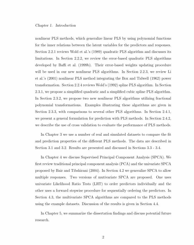
nonlinear PLS methods, which generalize linear PLS by using polynomial functions
for the inner relations between the latent variables for the predictors and responses.
Section 2.2.1 reviews Wold et al.’s (1989) quadratic PLS algorithm and discusses its
limitations. In Section 2.2.2, we review the error-based quadratic PLS algorithms
developed by Baffi et al. (1999b). Their error-based weights updating procedure
will be used in our new nonlinear PLS algorithms. In Section 2.2.3, we review Li
et al.’s (2001) nonlinear PLS method integrating the Box and Tidwell (1962) power
transformation. Section 2.2.4 reviews Wold’s (1992) spline PLS algorithm. In Section
2.3.1, we propose a simplified quadratic and a simplified cubic spline PLS algorithm.
In Section 2.3.2, we propose two new nonlinear PLS algorithms utilizing fractional
polynomial transformations. Examples illustrating these algorithms are given in
Section 2.3.3, with comparisons to several other PLS algorithms. In Section 2.4.1,
we present a general formulation for prediction with PLS methods. In Section 2.4.2,
we describe the use of cross validation to evaluate the performance of PLS methods.
In Chapter 3 we use a number of real and simulated datasets to compare the fit
and prediction properties of the different PLS methods. The data are described in
Section 3.1 and 3.2. Results are presented and discussed in Sections 3.3 - 3.4.
In Chapter 4 we discuss Supervised Principal Component Analysis (SPCA). We
first review traditional principal component analysis (PCA) and the univariate SPCA
proposed by Bair and Tibshirani (2004). In Section 4.2 we generalize SPCA to allow
multiple responses. Two versions of mutivariate SPCA are proposed. One uses
univariate Likelihood Ratio Tests (LRT) to order predictors individually and the
other uses a forward stepwise procedure for sequentially ordering the predictors. In
Section 4.3, the multivariate SPCA algorithms are compared to the PLS methods
using the example datasets. Discussion of the results is given in Section 4.4.
In Chapter 5, we summarize the dissertation findings and discuss potential future
research.
2

Chapter 2
Partial Least Squares
Partial Least Squares (PLS), also called “Projection to Latent Structures,” is a
relatively new biased regression modeling technique that was first developed and
used in economics by Herman Wold (Wold, 1966, 1975). It then became popular
in a number of application areas such as computational chemistry (chemometrics),
quantitative structure-activity relationships modeling, multivariate calibration, and
process monitoring and optimization. In the past four decades, PLS methodology
has been expanded beyond the initial linear NIPALS algorithm (Nonlinear Iterative
Partial Least Squares) developed by H. Wold and coworkers during the mid 1970s
(Eriksson et al., 1999). In the late 1980s to early 1990s, PLS was formulated in a
statistical framework (Hoskuldsson, 1988; Helland, 1990; Frank and Friedman, 1993).
de Jong (1993) developed a linear PLS algorithm, SIMPLS, in which the latent
variables are calculated directly rather than iteratively. Svante Wold, Herman’s
son, has probably made the most significant contributions to the PLS literature and
popularized PLS in computational chemistry. His work (Wold et al., 1989; Wold,
1992) on nonlinear PLS enabled PLS to fit highly nonlinear data. Later works by
Baffi et al. (1999b) and Li et al. (2001) modified Wold’s nonlinear PLS algorithms to
allow more flexible inner relationships. These later methods were shown to achieve
3
Chapter 2. Partial Least Squares
better fit and prediction with a number of datasets.
PLS emerged as a way to model ill-conditioned data for which the ordinary least
squares (OLS) regression is not appropriate. Suppose we have data matrices, X
and Y , with X being an N × P predictor matrix and Y being an N ×M response
matrix. If the goal is to predict Y from X, the simplest method to use is OLS
regression, where the underlying model is often written as Y = XB + E, where B
is the P ×M coefficient parameter matrix and the rows of E are usually assumed
to be independent identically distributed (i.i.d.) vectors of normal random errors.
When X is full rank, the parameter matrix can be estimated with the least squares
estimator: B = (X ′X)−1X ′Y . However, when the number of predictors is large
compared to the number of observations, X may be singular and the parameter
estimates are not unique. A solution is to reduce the dimension of X through latent
variable projections. Principal Component Analysis (PCA) is probably the most
popular approach taking this strategy. In PCA, much of the variance in X can
often be explained by a few orthogonal latent variables or components (often one or
two). The orthogonality of the principal components eliminates multicollinearity in
X. Then these few principal components can be used as new predictors in an OLS
regression with the response Y . Since the principal components are chosen to explain
X only, irrelevant information with regard to Y is also retained. PLS can be viewed
as a response to this weakness of PCA in that it extracts information that is relevant
to both Y and X through a simultaneous decomposition of both the response and
the predictor matrices.
4
Chapter 2. Partial Least Squares
2.1 Linear PLS: NIPALS and SIMPLS
Linear PLS decomposes X and Y in terms of sets of orthogonal factors and loadings.
In this following illustration of the basic structure of linear PLS, XN×P and YN×M
denote the centered (with mean 0) and scaled (with standard deviation 1) predictor
and response matrices.
A linear PLS model with A components has the form
XN×P = TN×AP′A×P + E
= [t1, t2, ..., tA]
p′1
p′2...
p′A
+ E
=A∑a=1
tap′a + E = t1p
′1 + t2p
′2 + · · ·+ tAp
′A + E,
and
YN×M = UN×AQ′A×M + F
= [u1, u2, ..., uA]
q′1
q′2...
q′A
+ F
=A∑a=1
uaq′a + F = u1q
′1 + u2q
′2 + · · ·+ uAq
′A + F,
where the columns of T and U (ta and ua for a = 1, 2, ..., A) are latent variables (also
called “factors” or “factor scores” in PLS) for X and Y , the columns of P and Q (pa
and qa for a = 1, 2, ..., A) are X and Y loading vectors, and E and F are residuals.
5
Chapter 2. Partial Least Squares
The latent variables ta and ua are constrained to be in the column space of X and
Y , respectively. That is, ta = Xwa and ua = Y ca for some wa and ca, and therefore
T = XW and U = Y C, where wa and ca are the ath column of W and C, respectively.
Different PLS algorithms estimate wa and ca differently through fulfilling certain
covariance maximization criteria with a number of constraints. Details about these
criteria and constraints for two of the most popular PLS algorithms, NIPALS and
SIMPLS, will be given in Sections 2.1.1 and 2.1.2.
Besides the decomposition of the data matrices, a linear relation is assumed
between each pair of the latent variables: ua = bata + ha, where ba is a constant and
ha denotes residuals. Write diag(B) as an A × A matrix containing b1, b2, ..., bA as
the diagonal elements and zeros as the other elements. This allows Y to be modeled
by T and Q as:
YN×M = TN×Adiag(B)A×AQ′A×M + F ∗
= [t1, t2, · · · , tA]
b1 0 · · · 0
0 b2 · · · ...... · · · . . . 0
0 · · · 0 bA
q′1
q′2...
q′A
+ F ∗
=A∑a=1
tabaq′a + F ∗ = t1b1q
′1 + t2b2q
′2 + ...+ tAbAq
′A + F ∗.
Letting q∗′a = baq
′a, we can rewrite this equation in regression form as
YN×M = t1q∗1′ + t2q
∗2′ + ...+ tAq
∗A′ + F ∗
=A∑a=1
taq∗a′ + F ∗
= TQ∗′ + F ∗
= XWQ∗′ + F ∗
= XBPLS + F ∗,
6
Chapter 2. Partial Least Squares
where BPLS = WQ∗′.
2.1.1 Iterative PLS algorithm: NIPALS
Herman Wold (1975) published the first PLS algorithm, which he named “Nonlinear
Iterative Partial Least Squares (NIPALS).” Although it is described as “nonlinear,”
the inner relation between the latent variables ua and ta is linear, thus we consider
NIPALS a linear PLS algorithm. The basic steps of NIPALS are described at the
end of this section in Table 2.1. In summary, NIPALS searches for the estimates of
the first pair of components t1 and u1 through iterative steps 2-8 in Table 2.1 and
it stops when the estimate of t1 does not change given some pre-specified tolerance.
Once t1 and u1 are obtained, the algorithm proceeds by deflating the data matrices
(Step 11) and repeats the iterative steps to obtain t2 and u2, and so on until the last
factor scores tA and uA are obtained.
Instead of estimating the X weights wa and Y weights ca directly, NIPALS esti-
mates weights w∗a and c∗a based on the deflated matrices Xa−1 and Ya−1. Therefore
in NIPALS the latent variables ta and ua are estimated as
ta = Xa−1w∗a and ua = Ya−1c
∗a.
Since C(Xa−1) ⊂ C(X) and ta = Xwa = Xa−1w∗a, we have wa = (X ′X)−1X ′Xa−1w
∗a.
Hence we can get the estimate of wa with wa = (X ′X)−1X ′Xa−1w∗a. Similarly, the
estimate of ca satisfies ca = (Y ′Y )−1Y ′Ya−1c∗a. Once we have the estimates for wa, ba
and qa, we can obtain the estimate of the PLS coefficient BPLS with BPLS = W Q∗′.
In Table 2.1, we use t(i)a , u
(i)a , w
∗(i)a and c
∗(i)a to denote the intermediate values
for the estimates of parameters ta, ua, w∗a and c∗a at the ith iteration, respectively,
7
Chapter 2. Partial Least Squares
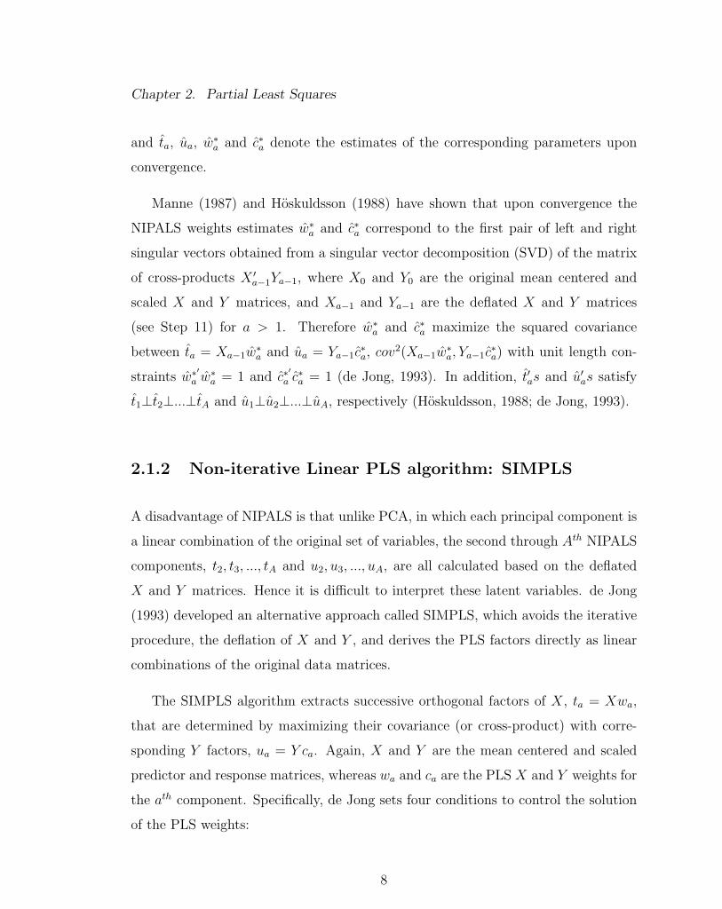
and ta, ua, w∗a and c∗a denote the estimates of the corresponding parameters upon
convergence.
Manne (1987) and Hoskuldsson (1988) have shown that upon convergence the
NIPALS weights estimates w∗a and c∗a correspond to the first pair of left and right
singular vectors obtained from a singular vector decomposition (SVD) of the matrix
of cross-products X ′a−1Ya−1, where X0 and Y0 are the original mean centered and
scaled X and Y matrices, and Xa−1 and Ya−1 are the deflated X and Y matrices
(see Step 11) for a > 1. Therefore w∗a and c∗a maximize the squared covariance
between ta = Xa−1w∗a and ua = Ya−1c
∗a, cov
2(Xa−1w∗a, Ya−1c
∗a) with unit length con-
straints w∗′a w∗a = 1 and c∗
′a c∗a = 1 (de Jong, 1993). In addition, t′as and u′as satisfy
t1⊥t2⊥...⊥tA and u1⊥u2⊥...⊥uA, respectively (Hoskuldsson, 1988; de Jong, 1993).
2.1.2 Non-iterative Linear PLS algorithm: SIMPLS
A disadvantage of NIPALS is that unlike PCA, in which each principal component is
a linear combination of the original set of variables, the second through Ath NIPALS
components, t2, t3, ..., tA and u2, u3, ..., uA, are all calculated based on the deflated
X and Y matrices. Hence it is difficult to interpret these latent variables. de Jong
(1993) developed an alternative approach called SIMPLS, which avoids the iterative
procedure, the deflation of X and Y , and derives the PLS factors directly as linear
combinations of the original data matrices.
The SIMPLS algorithm extracts successive orthogonal factors of X, ta = Xwa,
that are determined by maximizing their covariance (or cross-product) with corre-
sponding Y factors, ua = Y ca. Again, X and Y are the mean centered and scaled
predictor and response matrices, whereas wa and ca are the PLS X and Y weights for
the ath component. Specifically, de Jong sets four conditions to control the solution
of the PLS weights:
8

Chapter 2. Partial Least Squares
(1) Maximization of covariance: u′ata = c′a(Y′X)wa = max!
(2) Normalization of X weights wa: w′awa = 1.
(3) Normalization of Y weights ca: c′aca = 1.
(4) Orthogonality of X factors: t′bta = 0 for a > b.
The last constraint is necessary because without it there will be only one solution.
In particular, the X and Y weights for the first component, w1 and c1, can be
calculated as the first left and right singular vectors of the cross-product matrix
S0 ≡ X ′Y , but then the weights for the remaining components are not defined. The
last constraint requires for a > b:
t′bta = t′bXwa = (t′btb)p′bwa = 0⇒ p′bwa = 0
⇒ wa⊥pb
⇒ wa⊥Pa−1 ≡ [p1, ..., pa−1],
where pb is the loading vector for the bth X factor. Hence any later weights vector
wa, where a > 1, is orthogonal to all preceding loadings.
Let P⊥a−1 = IP −Pa−1(P ′a−1Pa−1)−1P ′a−1 be a projection operator onto the column
space orthogonal to Pa−1, i.e. all X loading vectors preceding pa. Then wa and ca can
be obtained from the SVD of P⊥a−1S0, i.e. the cross-product matrix after a loading
vectors have been projected out, or S0 projected onto a subspace orthogonal to Pa−1.
SIMPLS avoids deflating the X and Y matrices by deflating the cross-product
S0 = X ′Y instead. The deflation is achieved by Sa−1 = S0−Pa−1(P ′a−1Pa−1)−1P ′a−1S0
for a ≥ 2. In practice, Sa−1 is usually deflated from its predecessor Sa−2 by carrying
out the projection onto the column space of Pa−1 as a sequence of orthogonal projec-
tions. For this, an orthonormal basis for Pa−1, Va−1 ≡ [v1, v2, ..., va−1], is constructed
from a Gram-Schmidt orthonormalization of Pa−1, i.e., va−1 ∝ pa−1−Va−2(V ′a−2pa−1),
a = 3, ..., A starting with V1 = v1 ∝ p1. Thus the deflation of Sa−1 is obtained by
9
Chapter 2. Partial Least Squares
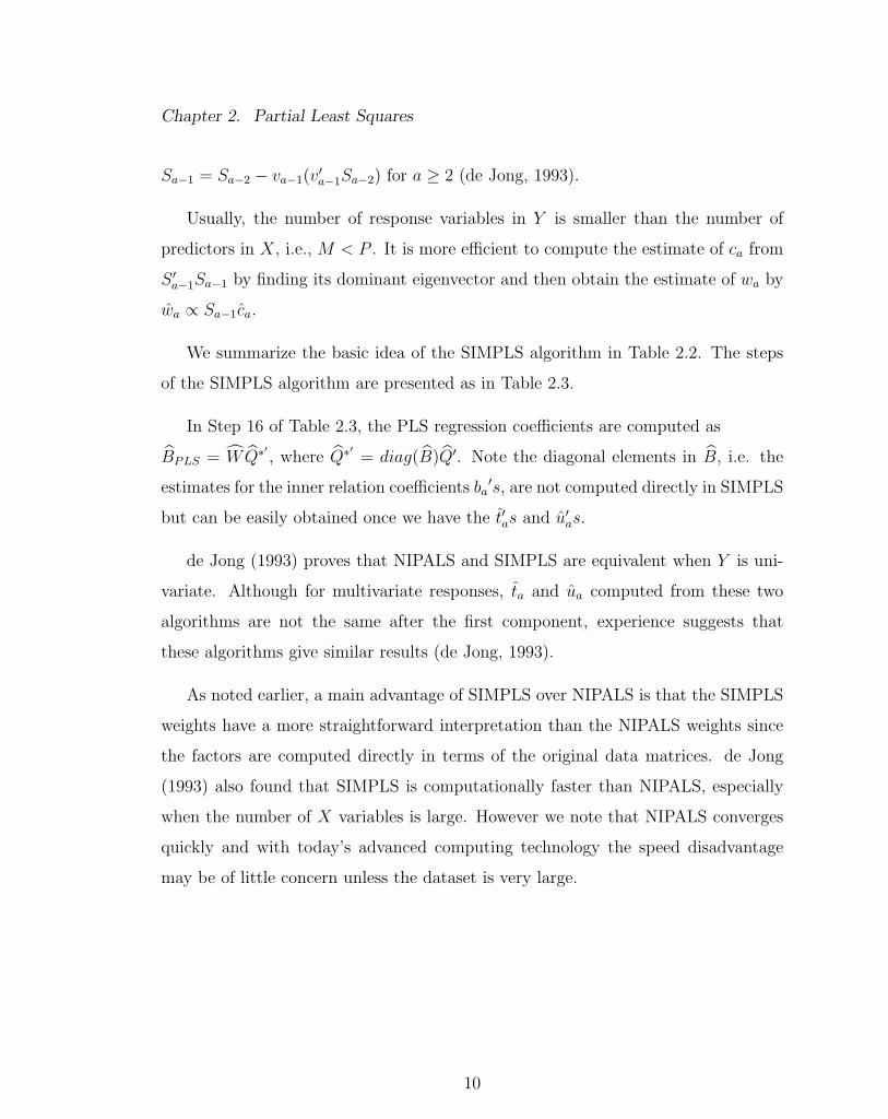
Sa−1 = Sa−2 − va−1(v′a−1Sa−2) for a ≥ 2 (de Jong, 1993).
Usually, the number of response variables in Y is smaller than the number of
predictors in X, i.e., M < P . It is more efficient to compute the estimate of ca from
S ′a−1Sa−1 by finding its dominant eigenvector and then obtain the estimate of wa by
wa ∝ Sa−1ca.
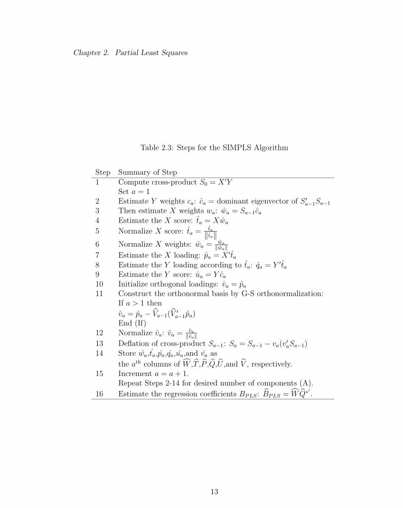
We summarize the basic idea of the SIMPLS algorithm in Table 2.2. The steps
of the SIMPLS algorithm are presented as in Table 2.3.
In Step 16 of Table 2.3, the PLS regression coefficients are computed as
BPLS = W Q∗′, where Q∗
′= diag(B)Q′. Note the diagonal elements in B, i.e. the
estimates for the inner relation coefficients ba′s, are not computed directly in SIMPLS
but can be easily obtained once we have the t′as and u′as.
de Jong (1993) proves that NIPALS and SIMPLS are equivalent when Y is uni-
variate. Although for multivariate responses, ta and ua computed from these two
algorithms are not the same after the first component, experience suggests that
these algorithms give similar results (de Jong, 1993).
As noted earlier, a main advantage of SIMPLS over NIPALS is that the SIMPLS
weights have a more straightforward interpretation than the NIPALS weights since
the factors are computed directly in terms of the original data matrices. de Jong
(1993) also found that SIMPLS is computationally faster than NIPALS, especially
when the number of X variables is large. However we note that NIPALS converges
quickly and with today’s advanced computing technology the speed disadvantage
may be of little concern unless the dataset is very large.
10

Chapter 2. Partial Least Squares
Table 2.1: Outline of the NIPALS Algorithm
Step Summary of Step0 Set X0 = X and Y0 = Y , where X and Y are centered and scaled.
Set a = 1.
1 Set i = 1 and initialize the Y factor scores u(i)a as the first column of Y ,
and initialize the X factor scores t(i)a as the first column of X.
2 Estimate X weight w∗(i)a by regressing Xa−1 on u
(i)a : w
∗(i)a =
X′a−1u(i)a
u(i)′a u
(i)a
.
3 Normalize w∗(i)a to unit length: w
∗(i)a = w
∗(i)a∥∥∥w∗(i)a
∥∥∥ .
4 Calculate X factor scores: t(i)a = Xa−1w
∗(i)a .
5 Calculate Y weights c∗(i)a by regressing Ya−1 on t
(i)a :c
∗(i)a =
Y ′a−1t(i)a
t(i)′a t
(i)a
.
6 Normalize c∗(i)a to unit length: c
∗(i)a = c
∗(i)a∥∥∥c∗(i)a
∥∥∥ .
7 Update u(i)a : u
(i)a = Ya−1c
∗(i)a .
8 Check convergence by examine the change in t(i)a ,
i.e.,∥∥∥t(i−1)a − t(i)a
∥∥∥ /∥∥∥t(i−1)a
∥∥∥ < ε, where ε is small, e.g., 10−6.
If no convergence, increment i = i+ 1 and return to Step 2.
Upon convergence, set ta = t(i)a , ua = u
(i)a , w∗a = w
∗(i)a , and c∗a = c
∗(i)a .
9 Estimate X and Y loadings by regressing Xa−1 on ta and
regressing Ya−1 on ua: pa =X′a−1 ta
t′a ta, qa =
Y ′a−1ua
u′aua.
10 Obtain the coefficient estimate between ua and ta by regressing ua on ta:
ba = u′a tat′a ta
.
11 Deflate Xa−1 and Ya−1 by removing the present component:
Xa = Xa−1 − tap′a and Ya = Ya−1 − batac∗
′a .
12 Increment a = a+ 1.Repeat Step 1 - 11 to give desired number of components.
11

Chapter 2. Partial Least Squares
Table 2.2: Basic idea of the SIMPLS Algorithm
Basic SIMPLS algorithmCenter and scale X and YObtain the cross-product S0 = X ′YFor a = 1, ..., Aif a = 1, compute SVD of S0
if a ≥ 2, compute SVD of Sa−1 = Sa−2 − va−1(v′a−1Sa−2)Estimate X weights wa = first left singular vector of SVD of Sa−1
Estimate X factor scores ta = XwaEstimate Y weights ca = Y ′ ta
t′a ta
Estimate Y factor scores ua = Y caEstimate X loadings pa = X ′ta/t
′ata
Store wa, ta, ua, and pa as the ath column of
W , T , U , and P , respectivelyEnd
12
Chapter 2. Partial Least Squares
Table 2.3: Steps for the SIMPLS Algorithm
Step Summary of Step1 Compute cross-product S0 = X ′Y
Set a = 12 Estimate Y weights ca: ca = dominant eigenvector of S ′a−1Sa−1
3 Then estimate X weights wa: wa = Sa−1ca4 Estimate the X score: ta = Xwa5 Normalize X score: ta = ta
‖ta‖6 Normalize X weights: wa = wa
‖wa‖7 Estimate the X loading: pa = X ′ta8 Estimate the Y loading according to ta: qa = Y ′ta9 Estimate the Y score: ua = Y ca10 Initialize orthogonal loadings: va = pa11 Construct the orthonormal basis by G-S orthonormalization:
If a > 1 then
va = pa − Va−1(V ′a−1pa)End (If)
12 Normalize va: va = va
‖va‖13 Deflation of cross-product Sa−1: Sa = Sa−1 − va(v′aSa−1)14 Store wa,ta,pa,qa,ua,and va as
the ath columns of W ,T ,P ,Q,U ,and V , respectively.15 Increment a = a+ 1.
Repeat Steps 2-14 for desired number of components (A).
16 Estimate the regression coefficients BPLS: BPLS = W Q∗′.
13
Chapter 2. Partial Least Squares
2.2 Nonlinear PLS with polynomial inner
relations
As in linear PLS, a nonlinear PLS model with A components has the form
X = TP ′ + E and Y = UQ′ + F , where P and Q contain the loading vectors for
X and Y , respectively, whereas T and U contain the latent variables ta and ua that
are constrained to be in the column space of X and Y , respectively, i.e., ta = Xwa
and ua = Y ca for some wa and ca. However instead of assuming that ua and ta are
linearly related, more flexible relationships will be allowed.
Linear PLS regression is very popular as it is a robust multivariate linear regres-
sion technique for the analysis of noisy and highly correlated data. However when
applied to data that exhibit significant non-linearity, linear PLS regression is often
unable to adequately model the underlying structure. Between the late 1980s and
early 2000s, researchers made great advances in integrating non-linear features within
the linear PLS framework. The goal was to produce nonlinear PLS algorithms that
retain the orthogonality properties of the linear methodology but were more capable
of dealing with nonlinearity in the inner relations. Among these new PLS meth-
ods, the most notable are the quadratic PLS algorithm (QPLS2) proposed by Wold
et al. (1989) and later modifications. These methods include Frank’s (1990) nonlin-
ear PLS (NLPLS) algorithm with a local linear smoothing procedure for the inner
relations, Wold’s (1992) spline PLS algorithm (SPL-PLS) with a smooth quadratic
spline function for the inner relations, and the error-based quadratic PLS algorithms
proposed by Baffi et al. (1999b). A fair amount of effort was also made in devel-
oping PLS algorithms using neural networks, which can approximate any continu-
ous function with arbitrary accuracy (Cybenko, 1989). Important neural network
PLS methods are Qin and McAvoy’s (1992) generic neural network PLS algorithm
(NNPLS), Holcomb and Morari’s (1992) PLS-neural network algorithm combining
14
Chapter 2. Partial Least Squares
PCA and feed forward neural networks (FFNs), Malthouse et al.’s (1997) nonlin-
ear PLS (NLPLS) algorithm implemented within a neural network, Wilson et al.’s
(1997) RBF-PLS algorithm integrating a radial basis function network, and Baffi et
al.’s (1999a) error-based neural network PLS algorithm. While neural network PLS
algorithms are popular, they are also criticized for having the tendency to over-fit
the data (Mortsell and Gulliksson, 2001), being not parsimonious, and unstable (Li
et al., 2001). We will not consider neural network methods here.
Another important nonlinear PLS algorithm is Li et al.’s (2001) Box-Tidwell
transformation based PLS (BTPLS). The BTPLS algorithm is attractive because it
provides a family of flexible power functions for modeling the PLS inner relation,
with linear and quadratic models as special cases. Secondly and probably more im-
portantly, BTPLS automatically selects the “best” power based on goodness-of-fit
of the data. Therefore, there is no need to pre-specify the exact functional form
for the PLS inner relation, as was necessary with fixed-order polynomial PLS algo-
rithms. This gives more flexibility and potentially more power for modeling data
with different levels of nonlinearity. According to Li et al. (2001), BTPLS is “a
compromise between the two extremes of the complexity spectrum of PLS, i.e., lin-
ear PLS and neural network PLS (NNPLS).” Compared to the neural network PLS
algorithms, BTPLS exhibits advantages in terms of both “computational effort and
model parsimony” (Li et al., 2001).
We note that from a statistical point of view, Wold’s quadratic PLS (QPLS2),
spline PLS (SPL-PLS), and the error-based PLS (PLS-C) are all fixed-order poly-
nomial PLS methods, in which the inner relations are still linear in the parameters.
Other methods, for example BTPLS, are nonlinear in the parameters. The term
“nonlinear” has been used in the literature to describe all of these methods. We
will follow the convention of referring to such extensions of NIPALS and SIMPLS as
nonlinear PLS, although the models used for the inner relation may or may not be
15
Chapter 2. Partial Least Squares
nonlinear in the parameters.
In this paper we will focus on nonlinear PLS models QPLS2, PLS-C, SPL-PLS
and BTPLS, which all adopt the original iterative linear PLS framework. As with
NIPALS, these algorithms estimate weights w∗a and c∗a based on the deflated data
matrices Xa−1 and Ya−1 rather than estimate PLS weights wa and ca directly. Once
w∗a and c∗a are estimated, the estimates for wa and ca can be obtained as previously
discussed for NIPALS, i.e. wa = (X ′X)−1X ′Xa−1w∗a and ca = (Y ′Y )−1Y ′Ya−1c
∗a. In
the following sections, we will first review and discuss the strengths and potential
problems for these models. We will then develop a simplified spline PLS model and
a PLS model that integrates a fractional polynomial based function for the inner
relation between the latent variables.
Throughout the rest of this thesis we will use a natural notation to denote
element-wise operations on the inner relation, the column vector ta and various data
matrices. For example,
t2a =
t2a1
t2a2
...
t2aN
,
and
X2a−1 =
X2a−1,11 X2
a−1,21 · · · X2a−1,P1
X2a−1,12 X2
a−1,22 · · · X2a−1,P2
... · · · . . ....
X2a−1,1N X2
a−1,2N · · · X2a−1,PN
,
where tai is the ith element of ta, and Xa−1,ji is the ith row and jth column element
of Xa−1.
16
Chapter 2. Partial Least Squares
2.2.1 Wold’s Quadratic PLS
In linear PLS, a first-order linear relation is assumed for the pairs of the latent
variables, i.e., for the ath component, ua = bata + ha, where ba is estimated by
least squares and ha denotes the residuals. The central idea behind a nonlinear PLS
method is to change this first-order linear inner relation to a higher-order polynomial
or nonlinear function so that more flexibility may be achieved.
If we rewrite the inner relation in a more general form:
ua = f(ta, βa) + ha,
where f(·) denotes an arbitrary polynomial function and βa is a vector of parame-
ters to be estimated, then we can modify the original linear PLS methods with the
hope that such methods are capable of modeling data with more complex curvature
characteristics.
Wold et al. (1989) proposed a quadratic PLS method QPLS2 by specifying the
inner relation as:
ua = βa0 + βa1ta + βa2t2a + ha,
i.e., a simple quadratic function for the ath PLS component.
The QPLS2 algorithm follows the same iterative scheme as NIPALS, i.e., com-
putes the parameters for one component at a time and upon convergence deflates the
data matrices and then repeats the computations for subsequent components. The
basic idea of QPLS2 is to project X and Y onto T and U with goals of (1) decompos-
ing X and Y as TP ′ and UQ′, respectively, with orthogonality among components;
and (2) satisfying the quadratic inner relation between ua and ta.
17
Chapter 2. Partial Least Squares
QPLS2 starts with a linearly initialized X weights estimate w∗a, and then up-
dates w∗a via a Newton-Raphson (Ypma, 1995) type linearization of the quadratic
inner relation. Vectors ta, qa, and ua are updated as in NIPALS. The inner relation
coefficients βa0, βa1 and βa2 are estimated through least squares. As with NIPALS,
ta is in the column space of X, however w∗a is derived from the correlation of ua with
a linear combination of ta and the quadratic term t2a.
A critical part of QPLS2 is the procedure for updating the X weights estimate
w∗a. Suppose we call the relation between latent variables ta and ua as the “inner
mapping,” and call the relation between ta and Xa−1 or between ua and Ya−1 as
the “outer mapping” (Baffi et al., 1999b). Then, using a higher order polynomial
function to relate each pair of latent variables affects the calculations of both the
inner mapping and the outer mapping because w∗a is derived from the covariance of
the ua scores with Xa−1. To take this into account, Wold et al. (1989) proposed a
procedure for updating w∗a by means of a Newton-Raphson linearization of the inner
relation function, i.e. a first-order Taylor series expansion of the quadratic inner
relation, and then solving it with respect to the weights correction. However, Wold’s
procedure for updating the w∗a is not straightforward and appears awkward. We will
not discuss QPLS2 further and the details of this algorithm can be found in Wold
et al. (1989).
2.2.2 Error-based quadratic PLS
Baffi et al. (1999b) proposed an alternative quadratic PLS algorithm (PLS-C) with an
updating method that we think is more sensible. Write the nonlinear inner relation
as ua = f(ta, βa) + ha, where ta = Xa−1w∗a and f(·, ·) is assumed to be an arbitrary
continuous function that is differentiable with regards to w∗a. Baffi et al. (1999b)
treat the coefficient βa as fixed and approximate ua = f(ta, βa) + ha by means of a
18

Chapter 2. Partial Least Squares
Newton-Raphson linearization:
ua = Ya−1c∗a ≈ f00 +
∂f
∂w∗a∆w∗a ⇒
Ya−1c∗a − f00 ≈
∂f
∂w∗a∆w∗a, (2.1)
where f00 denotes the fitted ua through the “inner mapping” at the current iteration,
∂f/∂w∗a is the partial derivative of the inner relation function with respect to w∗a,
and ∆w∗a denotes the weights correction. For PLS-C, the inner relation function is:
f(ta, βa) = βa0 + βa1t+ βa2t2a + ha.
Therefore f00 at the current iteration can be written as:
f(i)00 = β
(i)a0 + β
(i)a1 t
(i)a + β
(i)a2 t
(i)2a .
The partial derivative, defined as Z, is solved as:
Z = ∂f∂w∗a
= βa1Xa−1 + 2βa2(ta1′P ) ∗Xa−1,
where 1′P denotes a row vector of 1′s with length P (number of predictor variables),
and “∗” indicates element-wise multiplication. Therefore, in the last term of the
calculation of Z, (ta1′P ) ∗Xa−1 is
(ta1′P ) ∗Xa−1 =
ta1Xa−1,11 ta1Xa−1,21 · · · ta1Xa−1,P1
ta2Xa−1,12 ta2Xa−1,22 · · · ta2Xa−1,P2
... · · · . . ....
taNXa−1,1N taNXa−1,2N · · · taNXa−1,PN
.
In the calculation, ua = Ya−1c∗a in (2.1) is replaced with its estimate at the current
iteration u(i)a = Ya−1c
∗(i)a and then the estimate for ∆w∗a at the ith iteration, ∆w
∗(i)a , is
19

Chapter 2. Partial Least Squares
obtained by regressing u(i)a −f (i)
00 onto Z(i), which is obtained by plugging t(i)a and β
(i)a
into the derivative matrix Z. Baffi et al. (1999b) then update w∗(i)a by adding ∆w
∗(i)a .
The updating of w∗a is repeated iteratively until t(i)a = Xa−1w
∗(i)a converges according
to some pre-determined tolerance. Note u(i)a − f (i)
00 calculates the mis-match between
the estimates of ua at the ith iteration based on the “outer mapping” and the “inner
mapping.” This is why Baffi et al. (1999b) call their algorithm “the error-based
quadratic PLS algorithm.”
Baffi et al. (1999b) show that the error-based quadratic PLS algorithm (PLS-C)
performs better than QPLS2 in both goodness-of-fit and prediction. They observed
in their examples that PLS-C places more emphasis than QPLS2 toward explaining
the variability associated with Y rather than X. They claimed this might be because
the error-based input weights updating procedure omits the direct link between the
input weights w∗a and the output scores ta, and w∗a ceases to be directly linked to the
predictor matrix X. The weights correction ∆w∗a is in fact related directly to the
mismatch between ua and f00. This result may be desirable if prediction in Y is the
ultimate goal of the model.
The X weights updating procedure can be generalized to any inner relation,
provided the function is differentiable to the second order. The general error-based
w∗a weights updating steps are presented in Table 2.4. Table 2.5 gives a step-by-
step outline for general error-based nonlinear PLS algorithms without specifying a
particular inner relation for ta and ua. All later nonlinear PLS algorithms that we
will discuss essentially take the same steps. The differences only lie in the actual
Newton-Raphson linearization of the inner relation and the calculation of the partial
derivative matrix Z in the w∗a updating procedure for different inner relations.
20

Chapter 2. Partial Least Squares
Table 2.4: The error-based method for updating X weights w∗a.
Step Summary of Step1 Obtain the first order Taylor series expansion of
ua = Ya−1c∗a = f(ta, βa) + ha ≈ f00 + ∂f
∂w∗a∆w∗a.
Set f(i)00 = f(t
(i)a , β
(i)a ), i.e. f00 estimated at the current ith iteration.
Input t(i)a and β
(i)a into the partial derivative matrix Z = ∂f
∂w∗aand
denote the resulting matrix as Z(i). Set u(i)a = Ya−1c
∗(i)a .
2 Approximate the miss-match between u(i)a and f
(i)00 with
u(i)a − f (i)
00 = Z(i)∆w∗(i)a .
3 Estimate ∆w∗(i)a via least squares: ∆w
∗(i)a = (Z(i)′Z(i))−Z(i)′(u
(i)a − f (i)
00 ).
4 Update w∗(i)a with w
∗(i)a = w
∗(i)a + ∆w
∗(i)a .
21

Chapter 2. Partial Least Squares
Table 2.5: Steps in the error-based polynomial PLS algorithms.
Step Summary of Step0 Set X0 = X and Y0 = Y , where X and Y are centered and scaled.
Set a = 1.1 Set i = 1 and
initialize ua: u(i)a = the column of Ya−1 with the maximum variance.
2 Estimate X weights w∗a by regressing Xa−1 on u(i)a : w
∗(i)a =
X′a−1u(i)a
u(i)′a u
(i)a
.
3 Normalize w∗(i)a : w
∗(i)a = w
∗(i)a∥∥∥w∗(i)a
∥∥∥ .
4 Calculate X factor scores: t(i)a = Xa−1w
∗(i)a .
5 Set up the design matrix R for fitting the inner relation ua = f(ta, βa) + hwith least squares regression. The first column of R is a column of ones
and the remaining columns are the polynomial terms in t(i)a .
Compute β(i)a = (R′R)−1R′u
(i)a .
6 Set f(i)00 = f(t
(i)a , β
(i)a ).
7 Calculate Y loadings: q(i)a =
Y ′a−1f(i)00
f(i)′00 f
(i)00
.
8 Update u(i)a : u
(i)a = Ya−1q
(i)a
q(i)′a q
(i)a
, where q(i)a
q(i)′a q
(i)a
= c∗(i)a is the Y weights estimate.
9 Update the coefficients β(i)a with the updated u
(i)a by least squares.
10 Update w∗(i)a according to Table 2.4.
11 Normalize w∗(i)a to unit length: w
∗(i)a = w
∗(i)a∥∥∥w∗(i)a
∥∥∥ .
12 Update ta with the updated weights: t(i)a = Xa−1w
∗(i)a .
Update the design matrix R.
13 Check convergence by examining the change in t(i)a . If convergence,
move to Step 14, else increment i = i+ 1 and return to Step 5.
14 Set f00 = f(t(i)a , β
(i)a ), and obtain the final estimate of qa, ta, βa, ua and pa:
qa =Y ′a−1f00
f ′00f00, normalize qa with qa = qa
‖qa‖ ; ta = t(i)a ; βa = (R′R)−1R′u
(i)a ;
ua = f(ta, βa); and p′a = t′aXa−1
t′a ta.
15 Deflate X and Y by removing the present component:Xa = Xa−1 − tap
′a and Ya = Ya−1 − uaq
′a.
16 Increment a = a+ 1. Use deflated X and Y for additionalcomponents. Repeat Step 1 - 15.
22
Chapter 2. Partial Least Squares
2.2.3 The Box-Tidwell PLS algorithm
Box and Tidwell’s (1962) power transformation for linear regression has proved useful
in modeling nonlinear relationships. For a positive predictor x, the power transfor-
mation takes the following form:
ξ =
xα, if α 6= 0
ln(x), if α = 0.
Suppose the problem has a single response variable y and a single predictor vari-
able x. Instead of fitting the linear regression model
y = β0 + β1x+ e,
we fit a linear regression model between y and ξ:
y = f(ξ, β0, β1) + e = β0 + β1ξ + e = β0 + β1xα + e.
Clearly, the model with the transformed x is more flexible, with the linear model
as the special case α = 1. There are many other useful transformations such as the
square root (α = 1/2), the reciprocal (α = −1), the quadratic (α = 2), and the
natural logarithm (α = 0) of x. To estimate the unknown parameters β0, β1 and α,
Box and Tidwell used linearization of the function f with a first order Taylor series
expansion about an initial guess of α0 = 1:
E(y) = f(ξ, β0, β1) ≈ β0 + β1x+ (α− α0) {∂f(ξ; β0, β1)/∂α}α=α0= β0 + β1x+ γz,
23

Chapter 2. Partial Least Squares
where γ = (α− 1)β1 and z = xln(x). Box and Tidwell (1962) estimate α, β0 and β1
as follows:
(1) Obtain the least squares estimate of β1 in E(y) = β0 + β1x and denote the
estimate as β1.
(2) Obtain the least squares estimate of γ in E(y) = β0 + β1x+ γz as γ.
(3) Estimate α as α∗ = (γ/β1) + 1.
(4) Update the estimates of β0 and β1 by least squares in E(y) = β0 + β1ξ with ξ
defined using α = α∗.
After α∗, the estimate of α, from the first iteration is obtained, additional iter-
ations of step (1)-(4) follow by replacing the initial guess of α = 1 with α = α∗.
However, as Box and Tidwell (1962) noted, the procedure rapidly converges and of-
ten one iteration is satisfactory. Alternatively, non-linear least squares can be used
to estimate the parameter directly.
The Box-Tidwell transformation assumes x > 0. In PLS regression, the latent
variable ta has zero mean, which means that the Box-Tidwell transformation cannot
be applied directly to model the PLS inner relation. Therefore Li et al. (2001)
modified the Box-Tidwell procedure so that the transformed latent variable satisfies
(sgn(ta))δ|ta|α if α 6= 0 and (sgn(ta))
δln(|ta|) if α = 0, where in both cases δ = 0 or
1. Here sgn(ta) denotes the element-wise operation
sgn(ta) =
sgn(ta1)
sgn(ta2)...
sgn(taN)
,
and the sign function sgn(taj) is defined as
24
Chapter 2. Partial Least Squares
sgn(taj) =
1, if taj > 0
0, if taj = 0
−1, if taj < 0.
Additional modifications are needed since |taj|α is undefined when both taj = 0
and α < 0. Hence, α is constrained to be positive, i.e. α > 0. Therefore, the
regression model used for modeling the PLS inner relation can be written as:
ua = β0 + β1(sgn(ta))δ|ta|α + ha,
where |ta|α = ln(|ta|) if α = 0 for δ = 0 or 1.
To ensure α > 0, Li et al. (2001) define α = v2, where v is non-zero. They
estimate the parameters following the original Box-Tidwell procedure, except that g
is expanded with respect to v instead of α, using an initial guess v0 = 1. They then
linearize the model with a first-order Taylor series:
ua = β0 + β1(sgn(ta))δ|ta|v
2
≈ β0 + β1(sgn(ta))δ|ta|+ (v − v0)
{∂f(ta; β0, β1, δ, v
2)/∂v}v=v0
= β0 + β1(sgn(ta))δ|ta|+ 2(v − 1)β1(sgn(ta))
δ|ta|ln(|ta|)
= β0 + β1z1 + γz2
where γ = 2(v − 1)β1, z1 = (sgn(ta))δ|ta| and z2 = (sgn(ta))
δ|ta|ln(|ta|). Li et al.
(2001) estimate α, β0, β1 and γ using the following steps:
(1) Obtain the least squares estimate of β1 in
ua = β0 + β1(sgn(ta))δ|ta|+ ha
25

Chapter 2. Partial Least Squares
for both δ = 0 and δ = 1. Choose between δ = 0 and 1 based on which gives the
smaller residual sum of squares. Denote the corresponding estimate of β1 by β1.
(2) Obtain the least squares estimate of γ in
ua = β0 + β1(sgn(ta))δ|ta|+ γβ1(sgn(ta))
δ|ta|ln(|ta|) + ha
for both δ = 0 and δ = 1. Choose between δ = 0 and 1 based on which gives the
smaller residual sum of squares. Denote the corresponding estimate of γ by γ.
(3) Estimate α as α∗ = ((γ/2β1) + 1)2.
(4) Update the least squares estimates of β0, β1, and δ in
ua = β0 + β1(sgn(ta))δ|ta|α
∗+ ha
for both δ = 0 and δ = 1. Choose the set of estimates that gives the better fit and
denote these estimates as β∗0 , β∗1 and δ∗.
At each of the steps (1), (2) and (3), least squares is performed separately for
the two values of δ and the estimates with the better fit are selected. Also note that
only the results from the first iteration of Box-Tidwell procedure are used.
The BTPLS algorithm resembles the error-based quadratic PLS algorithm in that
it follows the same computational scheme as NIPALS and uses the error-based PLS
X weights updating procedure of Baffi et al. (1999b). The matrix of derivatives
Z = ∂f/∂w∗a is obtained for both δ = 1 and 0:
Z =
αβ1(|ta|(α−1)1′P ) ∗Xa−1 if δ = 1
αβ1(|ta|(α−1)1′P ) ∗ |Xa−1| if δ = 0 .
26
Chapter 2. Partial Least Squares
Li et al. (2001) proposed two versions of BTPLS. We described BTPLS(I). The
other version, BTPLS(II), contains a linear term for the inner relation:
ua = β0 + β1ta + β2(sgn(ta))δ|ta|α + ha.
BTPLS(II) includes BTPLS(I) as a special case (when β1 = 0). BTPLS(II) is more
flexible at the expense of an additional parameter. Li et al. (2001) suggest that
BTPLS(I) is preferable to BTPLS(II) when model simplicity is more important than
model fit for small datasets where data over-fitting is often an issue. However, we
did not see much difference in performance between these two algorithms for some
small and medium-sized datasets. We will provide results for BTPLS(I), which we
will refer to as “BTPLS” for simplicity.
Li et al. (2001) compared BTPLS with linear PLS, PLS-C and the error-based
neural network PLS (NNPLS) algorithms for several real and simulated datasets
with a high degree of nonlinearity. They conclude that BTPLS provides better fits
and predictions than linear and quadratic PLS for data with nonlinear features.
Compared to NNPLS, BTPLS is more computationally efficient, parsimonious and
stable.
Li et al. (2001) introduce a couple of “tricks” to ensure numerical stability of
BTPLS. In Step (2) of the modified Box-Tidwell procedure, observations with ta
values close to zero, say |taj| < ρ, where ρ is a small positive value, are eliminated
from the calculation. In addition, in Step (3), the estimated power α∗ is truncated
as follows:
α∗ =
αmin if ((γ/2β1) + 1)2 < αmin
αmax if ((γ/2β1) + 1)2 > αmax,
where αmin and αmax are preset boundary values.
27
Chapter 2. Partial Least Squares
Li et al. did not explicitly state what boundary values were used for their analysis.
Choices for ρ, αmin and αmax may be case-specific, i.e., different choices of these values
may affect the stability of the algorithm with different datasets. This was true in
our attempts to apply BTPLS to several datasets. In addition, although we have no
problem with truncating the estimated power, we are less comfortable with holding
out observations to allow the fitting of the power model.
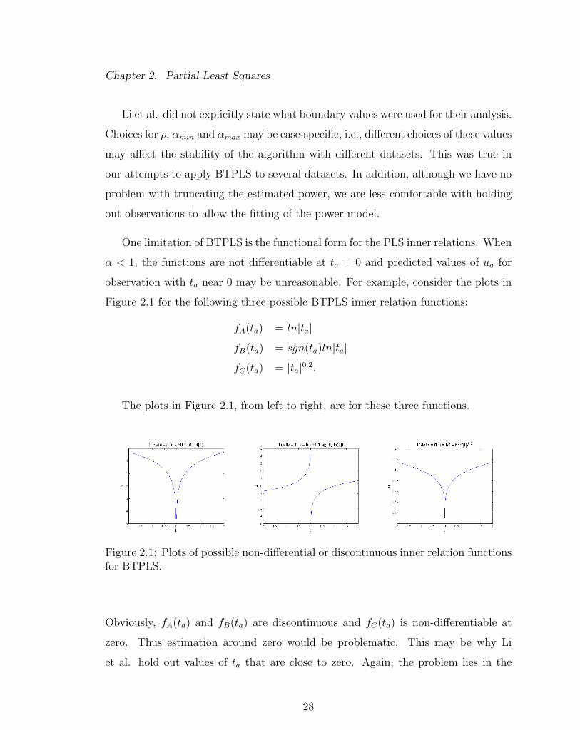
One limitation of BTPLS is the functional form for the PLS inner relations. When
α < 1, the functions are not differentiable at ta = 0 and predicted values of ua for
observation with ta near 0 may be unreasonable. For example, consider the plots in
Figure 2.1 for the following three possible BTPLS inner relation functions:
fA(ta) = ln|ta|
fB(ta) = sgn(ta)ln|ta|
fC(ta) = |ta|0.2.
The plots in Figure 2.1, from left to right, are for these three functions.
Figure 2.1: Plots of possible non-differential or discontinuous inner relation functionsfor BTPLS.
Obviously, fA(ta) and fB(ta) are discontinuous and fC(ta) is non-differentiable at
zero. Thus estimation around zero would be problematic. This may be why Li
et al. hold out values of ta that are close to zero. Again, the problem lies in the
28
Chapter 2. Partial Least Squares
functional form for the inner relation. It would be desirable to avoid such problems
by modifying the functional forms instead of modifying the data.
Another potential drawback of BTPLS is that the power α is estimated on a
continuous scale. Although this may make the modeling function very flexible, this
may also result in over-fitting, especially for small datasets or datasets with influential
observations.
2.2.4 Spline nonlinear PLS algorithms
Wold (1992) proposed a spline PLS algorithm (SPL-PLS), in which quadratic or
cubic functions are smoothly connected through a number of knots. The cubic spline
function used for modeling the PLS inner relation can be written as:
ua = β0 + β1ta + β2t2a + β3t
3a +
J∑j=1
bj+3(ta − zj)3+ + ha,
where zj is the jth knot (j = 1, 2, ..., J), and bj+3 denotes the coefficient for (ta−zj)3+
term, and the positive part function (x)+ is defined as
(x)+ =
x if x > 0
0 else.
The cubic term (ta − zj)3+ works exactly like a linear regression interaction term
between (ta − zj)3 and an indicator of whether ta − zj is positive.
In SPL-PLS, the number of the knots depends on the sample size and the knots
are selected so that each piece of the cubic curve contains approximately an equal
number of observations. SPL-PLS adapts a PLS input weights updating procedure
that is related to QPLS2, but we will omit the details. Other than the updating
procedure, there are a couple of specification issues that make SPL-PLS difficult
29

Chapter 2. Partial Least Squares
to implement. First, since estimates of the latent variables ua and ta change at
each iteration, it is difficult to pre-specify the location or number of knots for the
inner relation spline function. Wold (1992) suggests that the number of knots is
best estimated with cross validation, i.e., fit multiple spline models with different
number of knots and choose the “best” according to cross validation. This makes
the algorithm cumbersome and difficult to implement.
30
Chapter 2. Partial Least Squares
2.3 Simplified Spline and Fractional Polynomial
PLS
2.3.1 Simplified Spline PLS
We first propose a simplified version of the spline PLS algorithm that utilizes the
error-based PLS weights updating procedure and contains a single knot at zero. A
single knot at zero is parsimonious, and sensible because the t′as are linear combi-
nations of Xa−1, which is initially centered at zero. Hence the average value of ta is
approximately zero. This simplification eliminates the needs for specifying the num-
ber and location for knots according to the ta values, which are more “unknown”
to us than the original data. With one knot, we have two polynomials that are
connected smoothly at zero and such functions provide more flexibility than single
polynomial functions.
In particular, we propose quadratic (QSPLPLS) and cubic (CSPLPLS) spline
PLS algorithms. The inner relations for these two methods take the following forms:
(a) QSPLPLS: ua = s(ta) = β0 + β1ta + β2t2a + β3(ta − 0)2
+ + ha and
(b) CSPLPLS: ua = s(ta) = β0 + β1ta + β2t2a + β3t
3a + β4(ta − 0)3
+ + ha.
We fit these spline PLS models by following the computational procedure of the
other error-based polynomial PLS algorithms. Details of the procedure are presented
in Section 2.2.2. As before, the coefficients are estimated using least squares. The
matrices of partial derivatives Z = ∂s/∂w∗a for these two methods are
(a) QSPLPLS: Z = β1Xa−1 + 2β2(ta1′P ) ∗Xa−1 + 2β3[(ta)+1′P ] ∗Xa−1 and
(b) CSPLPLS: Z = β1Xa−1 +2β2(ta1′P )∗Xa−1 +3β3(t2a1
′P )∗Xa−1 +3β4[(ta)
2+1′P ]∗
Xa−1,
31
Chapter 2. Partial Least Squares
where in both cases, 1′P is a row vector of 1′s with length P , and “∗” denotes element-
wise multiplication.
2.3.2 Fractional Polynomial PLS
To overcome our concerns with BTPLS, we propose a new nonlinear PLS algorithm
that utilizes the fractional polynomial family and an error-based X weights updat-
ing procedure. Regression models using fractional polynomials of the predictors have
appeared in the literature for many years but was first formalized by Royston and
Altman (1994). Fractional polynomials can be viewed as a compromise between
fixed-order polynomials and the more flexible power models such as the Box-Tidwell
power model. The power terms of the fractional polynomials are restricted to a
handful of predefined set of rational values. The powers are selected so that the
conventional polynomials used in regression modeling are included. Through exam-
ples with a number of datasets, Royston and Altman (1994) show that fractional
polynomials often provide a better fit with fewer terms than conventional fixed-order
polynomials. They claim that fractional polynomials are “reasonably flexible, easy
to understand, parsimonious and, perhaps above all, are simple and quick to fit using
standard multiple-regression software” (Royston and Altman, 1994).
A fractional polynomial of degree m is defined as follows. For arbitrary powers
ψ1 ≤ ... ≤ ψm and positive values of X
φm(X; ξ, ψ) =m∑j=0
ξiHj(X),
where for j = 1, ...,m,
Hj(X) =
X(ψj) if ψj 6= ψj−1
Hj−1(X)lnX if ψj = ψj−1,
32
Chapter 2. Partial Least Squares
and H0(X) = 1 and ψ0 = 0.
Note
X(ψj) =
Xψj if ψj 6= 0
ln(x) if ψj = 0.
For X < 0, Royston and Altman (1994) suggest a simple transformation of X so
that the positivity requirement can be met. For example, one solution is to choose
a non-zero value ζ < X and rewrite the definition as
φm(X; ξ, ψ) =m∑j=0
ξiHj(X − ζ).
Royston and Altman (1994) found that models with m > 2 are rarely needed in
practice and fractional polynomials with m ≤ 2 offer many potential improvements
compared to traditional polynomials. They suggest that candidate values of the
power ψ include all powers from a fixed set
Ψ = {−2,−1,−0.5, 0, 0.5, 1, 2, ...,max(3,m)} .
They claim this specification is sufficiently rich to cover many practical cases ad-
equately. Obviously, fitting a fractional polynomial is simply fitting a number of
fixed-order polynomials.
Our motivation for developing a new PLS method comes from the potential prob-
lems of the BTPLS algorithm. Let us review these concerns. First, the modeling
functions are not continuous at ta = 0 for α < 1 and are non-differentiable at ta = 0
for 0 < α < 1. Second, the power parameter in BTPLS is estimated, so flexibility
may result in over-fitting, for example, when the dataset is small. Also, the power
α is constrained to be positive. Without this constraint, we may be able to find
33
Chapter 2. Partial Least Squares
better models with less effort. A PLS algorithm utilizing the fractional polynomials
may have potential for solving these problem. That is, it makes sense to fit a few
pre-selected polynomial models and select the one that fits the data best. In addi-
tion, we can use least squares for parameter estimation and linearization of nonlinear
functions is no longer needed. Thus the estimation is straightforward.
To overcome the first problem of BTPLS, we follow Royston and Altman’s (1994)
suggestion and shift ta linearly so that the shifted t′as are always positive. Specifically,
we first normalize ta:
t∗a = ta||ta|| ,
which guarantees that −1 ≤ taj/||ta|| ≤ 1 for the jth element of ta. Then for k > 0,
define
z1(t∗a) = k + kt∗a ∈ (0, 2k), and z2(t∗a) = k − kt∗a ∈ (0, 2k),
which are both centered at k. A natural choice is k = 1, which we use in subsequent
discussions.
We can fit fractional polynomials with z1(t∗a) or z2(t∗a). There is no obvious reason
to choose one over the other. We tried three possible functional forms using both
z1(t∗a) and z2(t∗a):
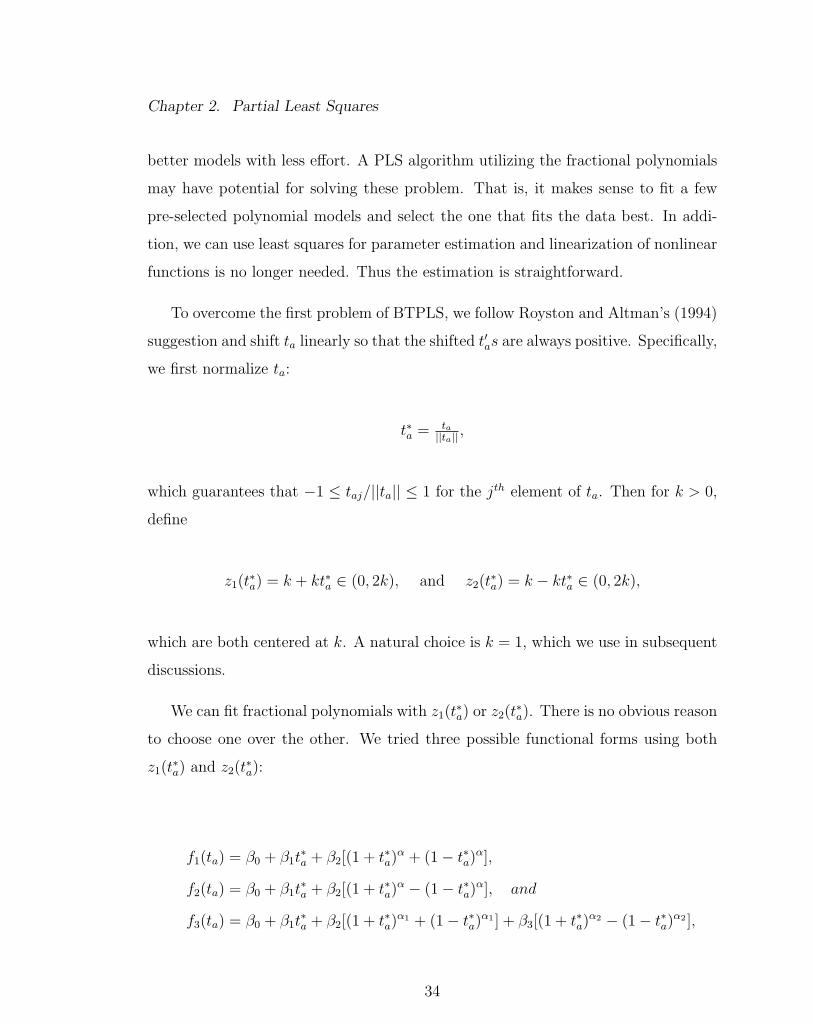
f1(ta) = β0 + β1t∗a + β2[(1 + t∗a)
α + (1− t∗a)α],
f2(ta) = β0 + β1t∗a + β2[(1 + t∗a)
α − (1− t∗a)α], and
f3(ta) = β0 + β1t∗a + β2[(1 + t∗a)
α1 + (1− t∗a)α1 ] + β3[(1 + t∗a)α2 − (1− t∗a)α2 ],
34
Chapter 2. Partial Least Squares
where
(1± t∗a)α =
ln(1± t∗a) if α = 0
(1± t∗a)ln(1± t∗a) if α = 1.
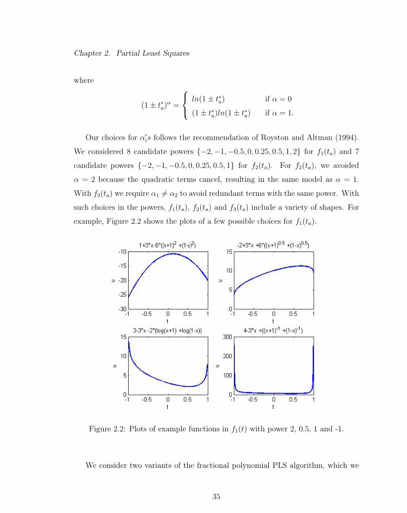
Our choices for α′is follows the recommendation of Royston and Altman (1994).
We considered 8 candidate powers {−2,−1,−0.5, 0, 0.25, 0.5, 1, 2} for f1(ta) and 7
candidate powers {−2,−1,−0.5, 0, 0.25, 0.5, 1} for f2(ta). For f2(ta), we avoided
α = 2 because the quadratic terms cancel, resulting in the same model as α = 1.
With f3(ta) we require α1 6= α2 to avoid redundant terms with the same power. With
such choices in the powers, f1(ta), f2(ta) and f3(ta) include a variety of shapes. For
example, Figure 2.2 shows the plots of a few possible choices for f1(ta).
Figure 2.2: Plots of example functions in f1(t) with power 2, 0.5, 1 and -1.
We consider two variants of the fractional polynomial PLS algorithm, which we
35
Chapter 2. Partial Least Squares
call the Modified Fractional Polynomial PLS algorithms I and II (MFPPLS-I and
MFPPLS-II). In MFPPLS-I, a series of 8, 7, or 8 × 7 − 7 = 49 polynomial PLS
models are fitted individually for each component, depending on whether f1(t), f2(t)
or f3(t) is used. Then the model with the best fit, i.e. the model with the minimum
residual sum of squares in ua is selected for that component. Our examples show that
f1(t) and f2(t) are less likely to lead to over-fitting than f3(t). In our summaries,
MFPPLS-I is based on f1(t). The results based on f2(t) are similar.
With MFPPLS-II, the “best” model is selected at each iteration of fitting the
inner relation. That is, in Step 5 of Table 2.6, all models are fitted in each iteration
and then they are compared. The model with the minimum residual sum of squares
is selected at that iteration, and then the algorithm moves to the next iteration.
Initially, MFPPLS-II showed convergence problems with the discrete set of powers.
The estimated parameters and latent variables may not be stable after a relatively
large number of iterations (e.g., 5,000) for some data. Often the estimated power
fluctuates dramatically between iterations and this contributes to the instability of
the latent variables. In retrospect, this may not be too surprising because the powers
are discrete. To avoid the jump in selected powers from iteration to iteration, we
changed the discrete power set to a continuous set. In practice, we use an equally
spaced, relative fine grid:
α1 ∈ [−2 : s : 2] and α2 ∈ [−2 : s : 1] for α1 6= α2,
where s is the spacing between two adjacent powers. The condition α1 6= α2 in
MFPPLS-II is necessary otherwise β2 and β3 are non-estimable.
After experimenting with the grid spacing, we decided on s = 0.1, i.e. 41 and 31
candidates for α1 and α2, respectively. This choice gives us sufficient continuity in
the powers so that convergence problems are avoided. Therefore, MFPPLS-II fits a
total of 41× 31− 31 = 1240 polynomial models at each iteration of the computation
36
Chapter 2. Partial Least Squares
and then picks the one with the best fit of ta and ua. Obviously this is a lot of
computation, but the algorithm runs quickly with small or medium sized datasets.
In our summaries, MFPPLS-II uses f3(ta) for the inner relation because it showed
better data fit and reasonable predictive ability.
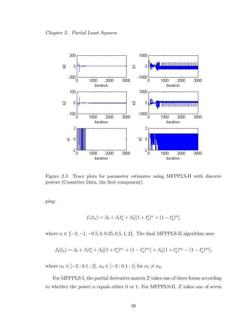
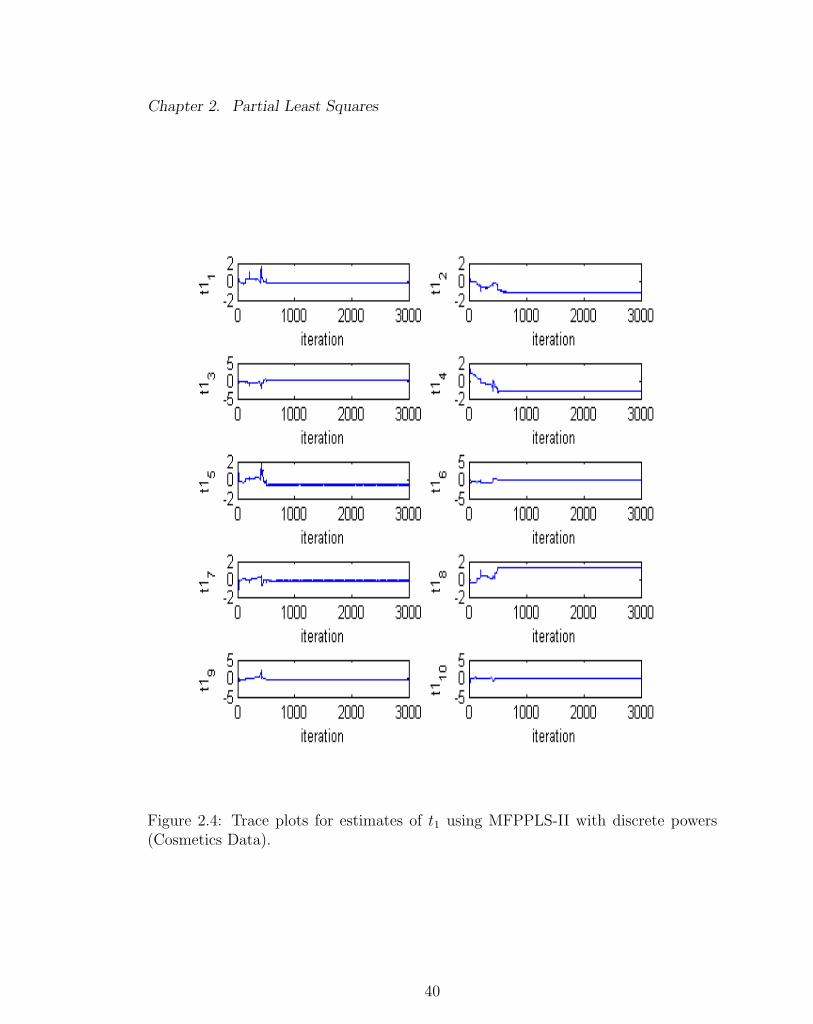
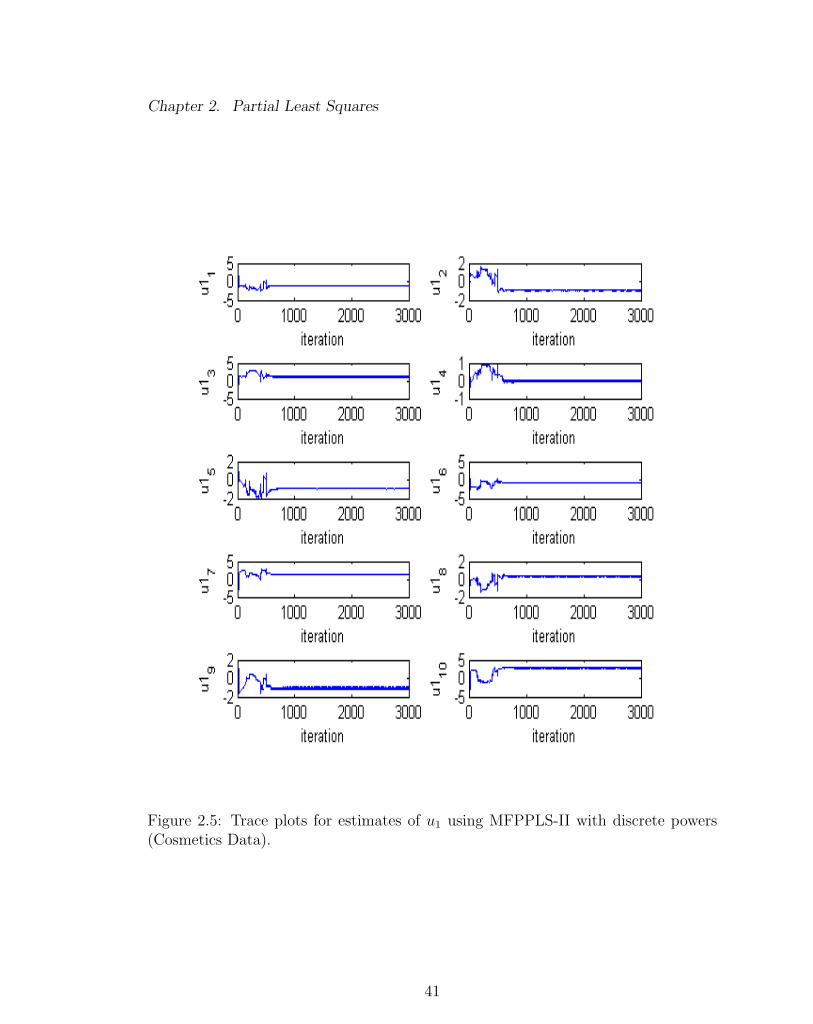
Figures 2.3 - 2.5 demonstrate an example of the convergence problem with using
MFPPLS-II with discrete powers. The convergence problem occurred with the second
component for the Cosmetics data. A description of the Cosmetics data will be
given in Section 2.3.3. Figure 2.3 shows the trace plots (i.e. iteration history) for the
estimates of parameters β0, β1, β2, β3, α1 and α2. Figure 2.4 and Figure 2.5 show the
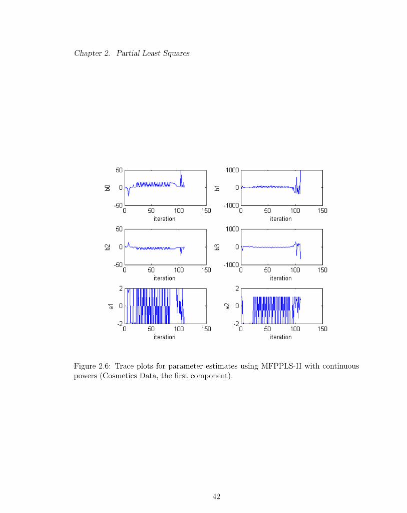
trace plots for the elements of the estimates for t1 and u1, respectively. Figures 2.6 -
2.8 give similar summaries for MFPPLS-II with continuous powers. The convergence
measure for ta (with an analogous measure for ua) is defined as
Dt =N∑n=1
(t(i)an − t(i−1)an )2/
N∑n=1
(t(i−1)an )2,
where t(i)an denotes the estimated value of ta at the ith iteration for the nth observation.
When discrete powers were used, the parameter estimates for β1, β3 and α2
had not converged after 3000 iterations (Figure 2.3), and neither had the estimated
elements of t1 and u1 (Figure 2.4 - 2.5). With a continuous sets of powers, the
estimated elements of t1 and u1 converged after about 200 to 300 iterations. Although
the parameter estimates may still be changing at the end of the 200 to 300 iterations,
we are not too concerned once ta and ua are stable, since the predicted values in Y are
calculated through the fitted values of ta and ua. Details for nonlinear PLS prediction
will be given in Section 2.4. Convergence problems were not observed with MFPPLS-
I. For fixed-order polynomial PLS models such as the error-based quadratic PLS and
the simplified spline PLS, the algorithms usually converges within 100 iterations.
In conclusion, our final MFPPLS-I algorithm uses f1 for the inner relation map-
37
Chapter 2. Partial Least Squares
Figure 2.3: Trace plots for parameter estimates using MFPPLS-II with discretepowers (Cosmetics Data, the first component).
ping:
f1(ta) = β0 + β1t∗a + β2[(1 + t∗a)
α + (1− t∗a)α],
where α ∈ {−2,−1,−0.5, 0, 0.25, 0.5, 1, 2}. The final MFPPLS-II algorithm uses
f3(ta) = β0 + β1t∗a + β2[(1 + t∗a)
α1 + (1− t∗a)α1 ] + β3[(1 + t∗a)α2 − (1− t∗a)α2 ],
where α1 ∈ [−2 : 0.1 : 2], α2 ∈ [−2 : 0.1 : 1] for α1 6= α2.
For MFPPLS-I, the partial derivative matrix Z takes one of three forms according
to whether the power α equals either 0 or 1. For MFPPLS-II, Z takes one of seven
38

Chapter 2. Partial Least Squares
forms according to whether one or both powers α1 and α2 equals either 0 or 1. Table
2.6 gives these expressions, where D = (||ta||Xa−1 − tata′Xa−1/||ta||)/||ta||2.
Table 2.6: Partial derivative matrix Z in MFPPLS-I and MFPPLS-II.
Power Z = ∂f∂w∗a
for MFPPLS-I
α = 0 [(β1 + β21
1+t∗a+ β2
11−t∗a
)1′P ] ∗D
α = 1 [(β1 + 2β2 + β2ln(1 + t∗a) + β2ln(1− t∗a))1′P ] ∗D
else [(β1 + αβ2(1 + t∗a)α−1 + αβ2(1− t∗a)α−1)1′P ] ∗D
Power Z = ∂f∂w∗a
for MFPPLS-II
α1 = 0, α2 = 1 [(β1 + β21
1+t∗a+ β2
11−t∗a
+ β3ln(1 + t∗a)− β3ln(1− t∗a))1′P ] ∗D
α1 = 1, α2 = 0 [(β1 + 2β2 + β2ln(1 + t∗a) + β2ln(1− t∗a) + β31
1+t∗a−β3
11−t∗a
)1′P ] ∗D
α1 = 0, α2 6= 1 [(β1 + β21
1+t∗a+ β2
11−t∗a
+ α2β3(1 + t∗a)α2−1
−α2β3(1− t∗a)α2−1)1′P ] ∗D
α1 6= 1, α2 = 0 [(β1 + α1β2(1 + t∗a)α1−1 + α1β2(1− t∗a)α1−1 + β3
11+t∗a
−β31
1−t∗a)1′P ] ∗D
α1 = 1, α2 6= 0 [(β1 + 2β2 + β2ln(1 + t∗a) + β2ln(1− t∗a) + α2β3(1 + t∗a)α2−1
−α2β3(1− t∗a)α2−1)1′P ] ∗D
α1 6= 0, α2 = 1 [(β1 + α1β2(1 + t∗a)α1−1 + α1β2(1− t∗a)α1−1 + β3ln(1 + t∗a)
−β3ln(1− t∗a))1′P ] ∗D
else [(β1 + α1β2(1 + t∗a)α1−1 + α1β2(1− t∗a)α1−1 + α2β3(1 + t∗a)
α2−1
−α2β3(1− t∗a)α2−1)1′P ] ∗D
39
Chapter 2. Partial Least Squares
Figure 2.4: Trace plots for estimates of t1 using MFPPLS-II with discrete powers(Cosmetics Data).
40
Chapter 2. Partial Least Squares
Figure 2.5: Trace plots for estimates of u1 using MFPPLS-II with discrete powers(Cosmetics Data).
41
Chapter 2. Partial Least Squares
Figure 2.6: Trace plots for parameter estimates using MFPPLS-II with continuouspowers (Cosmetics Data, the first component).
42

Chapter 2. Partial Least Squares
Figure 2.7: Trace plots for estimates of t1 using MFPPLS-II with continuous powers(Cosmetics Data).
43
Chapter 2. Partial Least Squares
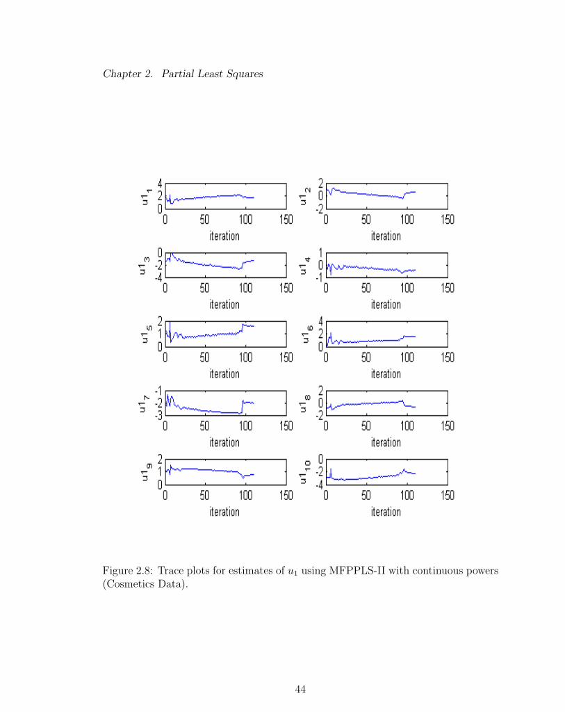
Figure 2.8: Trace plots for estimates of u1 using MFPPLS-II with continuous powers(Cosmetics Data).
44
Chapter 2. Partial Least Squares
2.3.3 Example
The Cosmetics data (Wold et al., 1989) will be used to illustrate MFPPLS-I and
MFPPLS-II. The data have been used by Wold et al. (1989), Baffi et al. (1999b) and
Li et al. (2001) to illustrate nonlinear PLS methods. The data were slightly altered
prior to publication to prevent the source and type of the 17 cosmetic cream formu-
lations used from being revealed (Wold et al., 1989). The formulations are composed
of P = 8 chemical constituents such as glycerin, water, emulsifier, and vaseline. In
a test of the quality of these creams, each cream has been applied to one half of
the face of each of 10 women models, while at the same time a “standard cream”
has been applied to the other half of the face. Then judges, including both trained
evaluators and the models, gave their scores for the M = 11 different quality indica-
tors such as “ease of application,” “greasiness,” “skin smoothness,” “skin shininess,”
and “overall appeal,” relative to the “standard cream.” The responses from the 10
models were averaged. Hence the data consist a 17 × 11 response matrix (Y ) and
a 17 × 8 predictor matrix (X). The purpose of the study was to develop a model
relating the cream composition (X) to the quality indicators (Y ). This model can
hopefully lead to the formulation of an “optimal” cream by choosing the appropriate
composition.
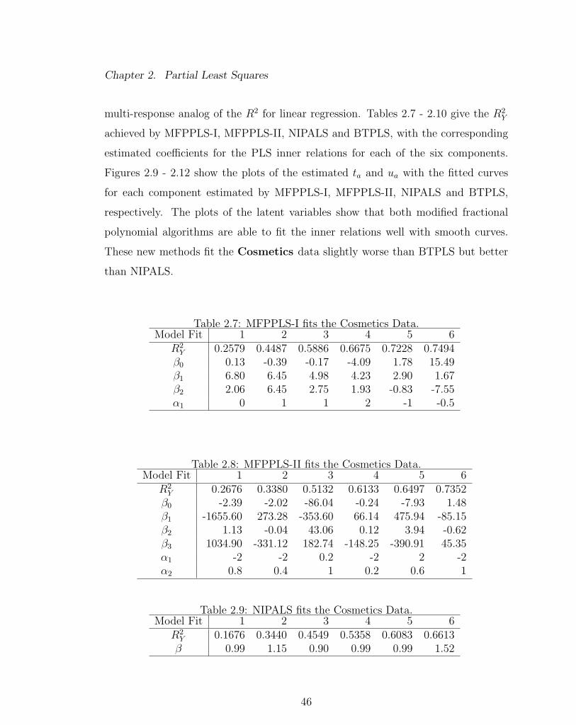
MFPPLS-I and MFPPLS-II were applied to the Cosmetics data, each using six
components. Both algorithms fit the data better than linear PLS methods. We mea-
sured the goodness-of-fit with the total variance explained over all response variables,
which is defined as:
R2Y = 1−
∑mi{Ymi−Ymi}2∑mi{Ymi−Y m.}2 ,
where Ymi and Ymi are the actual and fitted values of the ith observation of the
mth response variable, and Y m. is the mean value of the mth response. R2Y is the
45
Chapter 2. Partial Least Squares
multi-response analog of the R2 for linear regression. Tables 2.7 - 2.10 give the R2Y
achieved by MFPPLS-I, MFPPLS-II, NIPALS and BTPLS, with the corresponding
estimated coefficients for the PLS inner relations for each of the six components.
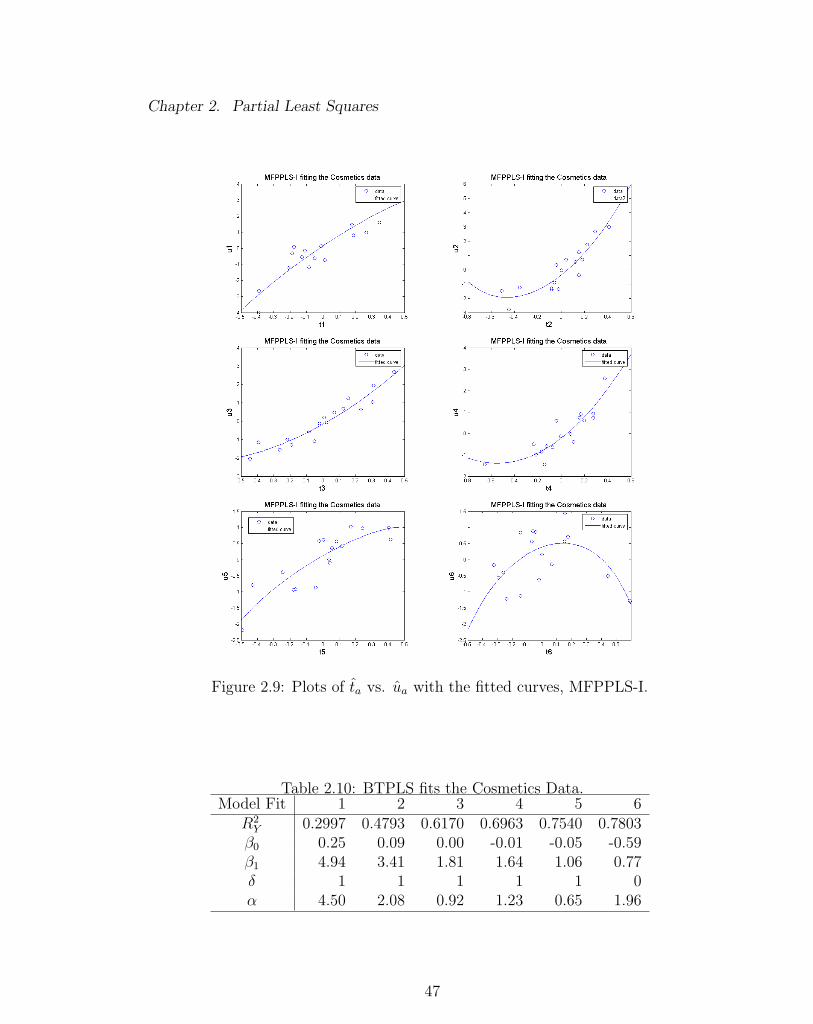
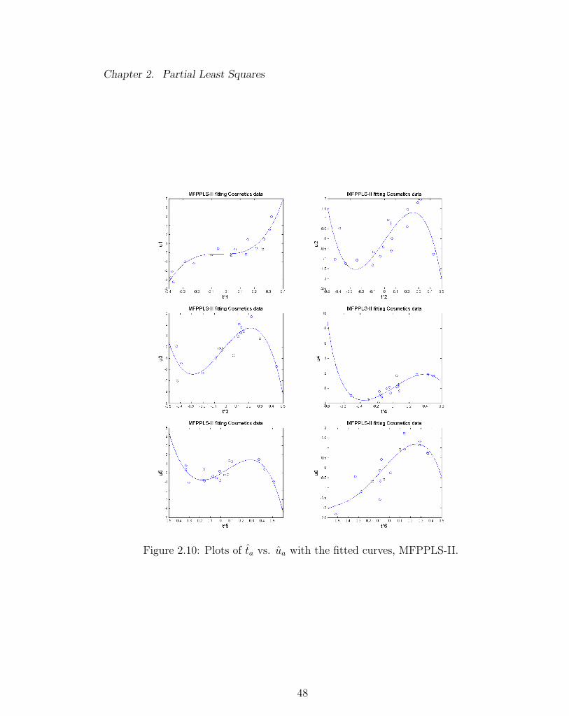
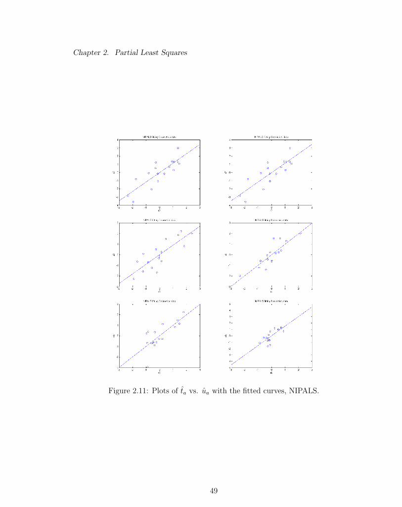
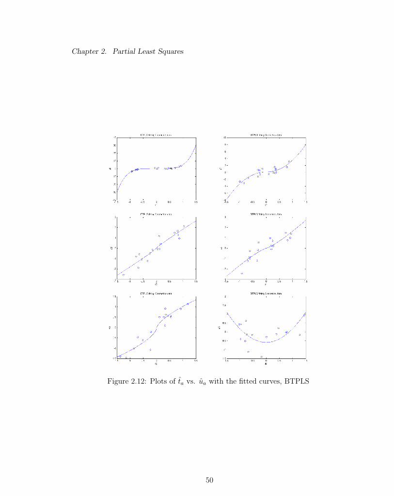
Figures 2.9 - 2.12 show the plots of the estimated ta and ua with the fitted curves
for each component estimated by MFPPLS-I, MFPPLS-II, NIPALS and BTPLS,
respectively. The plots of the latent variables show that both modified fractional
polynomial algorithms are able to fit the inner relations well with smooth curves.
These new methods fit the Cosmetics data slightly worse than BTPLS but better
than NIPALS.
Table 2.7: MFPPLS-I fits the Cosmetics Data.Model Fit 1 2 3 4 5 6
R2Y 0.2579 0.4487 0.5886 0.6675 0.7228 0.7494β0 0.13 -0.39 -0.17 -4.09 1.78 15.49β1 6.80 6.45 4.98 4.23 2.90 1.67β2 2.06 6.45 2.75 1.93 -0.83 -7.55α1 0 1 1 2 -1 -0.5
Table 2.8: MFPPLS-II fits the Cosmetics Data.Model Fit 1 2 3 4 5 6
R2Y 0.2676 0.3380 0.5132 0.6133 0.6497 0.7352β0 -2.39 -2.02 -86.04 -0.24 -7.93 1.48β1 -1655.60 273.28 -353.60 66.14 475.94 -85.15β2 1.13 -0.04 43.06 0.12 3.94 -0.62β3 1034.90 -331.12 182.74 -148.25 -390.91 45.35α1 -2 -2 0.2 -2 2 -2α2 0.8 0.4 1 0.2 0.6 1
Table 2.9: NIPALS fits the Cosmetics Data.Model Fit 1 2 3 4 5 6
R2Y 0.1676 0.3440 0.4549 0.5358 0.6083 0.6613β 0.99 1.15 0.90 0.99 0.99 1.52
46
Chapter 2. Partial Least Squares
Figure 2.9: Plots of ta vs. ua with the fitted curves, MFPPLS-I.
Table 2.10: BTPLS fits the Cosmetics Data.Model Fit 1 2 3 4 5 6
R2Y 0.2997 0.4793 0.6170 0.6963 0.7540 0.7803β0 0.25 0.09 0.00 -0.01 -0.05 -0.59β1 4.94 3.41 1.81 1.64 1.06 0.77δ 1 1 1 1 1 0α 4.50 2.08 0.92 1.23 0.65 1.96
47
Chapter 2. Partial Least Squares
Figure 2.10: Plots of ta vs. ua with the fitted curves, MFPPLS-II.
48
Chapter 2. Partial Least Squares
Figure 2.11: Plots of ta vs. ua with the fitted curves, NIPALS.
49
Chapter 2. Partial Least Squares
Figure 2.12: Plots of ta vs. ua with the fitted curves, BTPLS
50
Chapter 2. Partial Least Squares
2.4 PLS Prediction and Cross Validation
2.4.1 Obtaining PLS Predictions
The regression coefficient matrix BPLS can be readily computed for NIPALS and
SIMPLS as BPLS = W Q∗′, where Q∗
′= diag(B)Q′. W is the estimated X weight
matrix; B is a diagonal matrix containing the estimates of the PLS inner relation
coefficients as the diagonal elements; and Q is the estimated normalized Y loading
matrix. To predict the response for a new observation with X = X~, we first obtain
the predicted values on the standardized scale:
Y ~0 = X~
0 BPLS,
where X~0 is the X~ vector scaled and centered using the mean and standard devi-
ation from the X matrix used for the PLS fit. Next we transform Y ~0 to its original
scale:
Y ~m = (Y ~
0m + Y m)std(Ym),
where Y m and std(Ym) are the mean and standard deviation of the mth response
variable Ym, both computed with the data used to fit the model.
For the other PLS algorithms discussed in this thesis, the prediction is done
for each component, and then the results are summed to obtain the final predicted
values. In particular, we calculate the PLS X latent variable values t~a sequentially
for components a = 1, 2, ..., A. For the first component, t~1 = X~0 w∗1, and then
we continue the calculation with t~a = X~a−1w
∗a, where X~
a−1 = X~a−2 − t~a−1p
′a−1 for
a = 2, 3, ..., A. Once t~a is calculated, we obtain the predicted output latent variable
value with
51
Chapter 2. Partial Least Squares
u~a = fa(t
~a ; βa),
where fa(t~a ; βa) is the fitted inner relation for the ath component with parameter
estimates βa. The predicted response is calculated as
Y ~0 =
A∑a=1
u~a q′a,
where qa is the estimated ath Y loading vector from the PLS model. Lastly, we
transform Y ~0 back to the original response scale.
2.4.2 Model Selection and Validation with Cross Validation
An important aspect of fitting PLS models is to determine the number of components.
More components improve the fit to the data, but at the potential risk of over-fitting,
i.e., getting a well fitting model with little prediction power. The decision of the
“best” number of components with a good balance between model fit and predictive
power is often made with cross validation (Wold, 1982; Hoskuldsson, 1988; Wold
et al., 2001; Eriksson et al., 1999).
Ideally, we should test the prediction accuracy of a model with a separate vali-
dation set that is not used in the model building process. In such cases, the dataset
used for model building is often referred to as a “training set,” and the validation
set is called a “test set.” However, this may not be always possible as collecting
high dimensional data is often costly. Therefore researchers may not have sufficient
data to split into a test set and a training set. If this is the case, cross validation
provides a sensible alternative to evaluate how well a model predicts new data. Good
discussions of cross validation can be found in Wakeling and Morris (1987), Denham
(1997), Hastie et al. (2001), and Wold et al. (2004).
52
Chapter 2. Partial Least Squares
Cross validation is generally carried out by dividing the full dataset into a number
of approximately equal sized subsets, say, five to 10, and then one subset is held out
at a time while the remaining data are used to build the model. Once the model
is fit, predicted values of the held out cases are calculated. The squared difference
between the observed and predicted response is calculated and aggregated to give
the predictive sum of squares, PRESS. This is repeated so that each subset is held
out once and only once. This procedure is called “V-fold cross validation,” where V
is the number of subsets. Leave-One-Out cross validation (LOOCV) corresponds to
V = N , the total sample size of the full dataset. The PRESS statistic is defined as:
PRESS =∑
mi (Ymi − Y(mi))2,
where Y(mi) is the predicted value of Ymi based on the model fit to the (V −1) subsets
that exclude Ymi.
A relatively small PRESS indicates good predictive power of a PLS model. A few
other diagnostic measures based on PRESS are popular for measuring PLS models’
predictive power. These measures include Q2 (Wold, 1982), Eriksson’s (1999) total
CV criteria, and the Root Mean Square Prediction Error (RMSPE). The Q2, also
called “the goodness of prediction” or “the prediction variation” (Eriksson et al.,
1999), is defined as follows:
Q2 = 1−∑
mi{Ymi−Y(mi)}2∑mi{Ymi−Y (m.)}2
= 1− PRESS∑mi{Ymi−Y (m.)}2
,
where∑
mi
{Ymi − Y (m.)
}2is the sum of squared differences between the observed
responses and the mean responses calculated from the data less the held out ob-
servations. Q2 can be large negative but converges to R2Y in probability (Quan,
1988).
Eriksson’s (1999) total CV criterion is defined as:
53
Chapter 2. Partial Least Squares
CV = PRESS/(N − A− 1),
where N is the sample size and A is the number of components. Clearly CV attempts
to penalize a model for the number of components. Eriksson et al. (1999) suggest
choosing the model with the smallest CV . However, when N gets large, the penalty
effect diminishes.
RMSPE is a scaled measure of prediction error defined as
RMSPE =√PRESS/[(N − 1)M ],
where M is the number of response variables. A smaller RMSPE indicates a “better”
model.
We will use R2Y and Q2 to compare strength in goodness-of-fit and prediction
for competing PLS models, respectively, and use CV and RMSPE to determine the
number of components in a given PLS model.
A number of cross validation procedures have been implemented in PLS packages.
For example, the PLS procedure in SAS provides LOOCV and V-fold cross validation
and computes the PRESS statistic.
54
Chapter 3
A Comparison of PLS methods
Seven PLS algorithms were compared in terms of data fitting and prediction. These
algorithms include linear PLS (NIPALS/SIMPLS), the error-based quadratic PLS
algorithm (PLS-C), the Box-Tidwell PLS algorithm (BTPLS), the two simplified
spline PLS algorithms (QSPLPLS and CSPLPLS), and the two fractional polynomial
PLS algorithms (MFPPLS-I and MFPPLS-II). Nine small to large sized datasets
and two large simulated nonlinear datasets were used for the comparison. For each
method, models with one to five components were fit to these datasets, unless the
total response variance was explained before the fifth component, i.e., R2Y = 1.
LOOCV was used for the small to medium sized real data (N ≤ 60) and five-fold cross
validation was used for one large sized (N = 215) real and the two simulated datasets
(N = 500). With V-fold cross validation, results vary with the data splitting. We
ran the five-fold cross validation 10 times for each model and averaged the results.
The strength and weakness of each PLS method will be discussed.
Our tests with various data revealed that the nonlinear PLS methods often make
poor predictions on test data with “outlying” values in the input latent variable,
i.e., extremely small or large fitted values of t~a . This is not surprising since the
55
Chapter 3. A Comparison of PLS methods
extrapolation with high degree polynomials can often be risky. One possible solution
is to base prediction for new observations by restricting the calculated t~a values
within the range of ta obtained from the model fit. That is, if t~a < min(ta) then
set t~a = min(ta), and if t~a > max(ta) then set t~a = max(ta). These truncated t~a
values are then used in the prediction calculations. The truncation of t~a improved
the predictive ability (expressed in Q2) noticeably for all six nonlinear PLS methods
with almost all the datasets tested. The same truncation was also applied to the
linear PLS methods, which are less affected by extreme cases.
We chose NIPALS instead of SIMPLS for the comparisons because it is more
straightforward to obtain predictions based on truncating the extreme t~a values in
cross validation. The two algorithms typically gave similar conclusions.
3.1 Real Data
The sample sizes of the nine real-world datasets vary from seven to 215. All these
datasets have been used either to illustrate certain PLS algorithms or other multi-
variate methods. The Cosmetics data has been described in Section 2.3.3. The
other eight datasets are described as follows.
The Lung Toxicity data is described in McDonald et al.’s article (2004) inves-
tigating the relationship between composition and toxicity of motor vehicle emission
samples. The study used both PCA and linear PLS methods to fit the data, which
contains 11 response variables and 68 predictor variables on seven samples. The
predictor variables are measures of the particle and semi-volatile organic chemical
constituents from five groups of motor vehicles, including “normal-emitting” gasoline
vehicles, “normal-emitting” diesel vehicles, “high-emitting” gasoline vehicles emit-
ting white or black smoke, and “high-emitting” diesel vehicles. The emission sam-
ples were measured at both room temperature and at approximately 30 degrees
56
Chapter 3. A Comparison of PLS methods
Fahrenheit for two “normal-emitting” groups. The measures were then averaged
over samples within each vehicle group. Therefore, there are a total of seven sam-
ples (McDonald et al., 2004). The response variables are 11 laboratory measures of
toxicity measured from inflammation and tissue damage in rat lungs.
The Aroma data was used by Frank and Kowalski (1984) for predicting wine
quality and geographic origin from chemical measurements. It can also be found
in an SAS example for the PLS procedure. The data are from 37 Pinot Noir wine
samples, each described by 17 elemental chemical concentrations (Cd, Mo, Mn, Ni,
Cu, Al, Ba, Cr, Sr, Pb, B, Mg, Si, Na, Ca, P, K) and a score of the wine’s aroma
(the response) given by a panel of judges.
The Sea Water data are originally from Lindberg et al.’s (1983) linear PLS
analysis of spectrofluorimetric data on mixtures of humic acid and ligninsulfonate.
It is also available from the SAS Documentation. The data contain 27 spectra of sea
water, and three compounds in 16 samples from the Baltic Sea. The predictors are
the emission intensities at different frequencies in the spectrum. The responses are
the amounts of the three chemicals in the sample.
The Penta data come from the field of drug discovery and were used as a
SAS example data illustrating the PLS procedure. The dataset contains 30 samples
with 15 chemical measurements, which include size, lipophilicity, and polarity at
various sites on the molecule, and a measurement of the activity of the compound,
represented by the logarithm of the relative Bradykinin activating activity. The data
were used to develop a model to predict the compound’s biological activity from these
chemical measurements.
The Acids data, originally reported in McAvoy and Chamberlain (1989), are
available from the SAS Documentation. The data consist of spectrographic readings
on 33 samples containing known concentrations of two amino acids, tyrosine and
57
Chapter 3. A Comparison of PLS methods
tryptophan. The predictor variables are the measured spectra at 30 frequencies across
the range of frequencies. The response variables are the logarithms of the tyrosine
and tryptophan concentrations, and the logarithm of the total concentration.
The Jinkle data are provided to us by Jinkle Seagrave at the Lovelace Respiratory
Research Institute, Albuquerque, New Mexico. The data contain seven samples with
eight acute lung responses in rats and 24 chemical compositional measurements. The
goal is to build a model using these chemical measurements to predict the acute lung
responses.
The Mortality data, which appeared in McDonald and Schwing (1973), have
been popular in regression applications. The data contain 60 samples with measures
of U.S. mortality rates and 15 predictor variables including air pollution, weather,
population and socioeconomic variables. The goal is to relate air pollution and
confounders to mortality.
The Tecator data contain information on 215 samples of finely chopped pure
meat with different moisture, fat and protein contents. These three measurements
are the response variables. The predictor variables are 100 highly correlated mea-
surements from a spectrum of absorbances, recorded on a Tecator Food Analyzer.
The Tecator data have been used for neural network modeling and are available at
http://lib.stat.cmu.edu/datasets/tecator.
3.2 Simulated Non-Linear Data
Two simulated non-linear datasets, Sim A and Sim B, were generated. Each dataset
contains 500 samples with one response and four predictor variables. Sim A was
generated according to Baffi et al. (1999), i.e., x1, x2, x3, and x4 are mutually inde-
pendent uniformly distributed in [−0.25, 0.25] and Y = exp(2x1 sin(πx4))+sin(x2x3).
58
Chapter 3. A Comparison of PLS methods
Sim B was generated according to Li et al. (2001), i.e., x1, x2, x3, and x4 are mutually
independent uniformly distributed in [−0.25, 0.25] and Y = sinh(25x3) cos(x4)/30 +
50x2 sin(x1).
Baffi et al. (1999b) showed that PLS-C works well with Sim A, while Li et al.
(2001) showed that BTPLS works well with Sim B.
3.3 Results
Tables 2.11 - 2.21 summarize the results of the comparison with the selected datasets.
For the Cosmetics data, all nonlinear PLS algorithms fitted the data better
than NIPALS. QSPLPLS and CSPLPLS gave the best fit, both explaining about
30 - 80% of the total variance in responses with one to five components. The other
nonlinear PLS algorithms performed similarly and achieved slightly lower R2Y ’s than
the spline algorithms. Although NIPALS did not fit as well as the nonlinear algo-
rithms, it showed less over-fitting and is the only algorithm to be able to predict
the Cosmetic data. The five component NIPALS model achieved the highest Q2
of 0.15. All nonlinear PLS algorithms suffered from over-fitting and made poor pre-
dictions. Except for the one component BTPLS model (Q2 = 0.02), all nonlinear
PLS models have Q2 < 0. RMSPE chose a five components NIPALS model, a three
components PLS-C model, and all the other nonlinear models with one component.
CV picked the three components NIPALS model as the “best” linear PLS model and
one component models for all nonlinear methods.
The nonlinear PLS methods gave similar goodness-of-fit on the Lung Toxicity
data. All one component nonlinear models have R2Y ’s around 0.9 whereas the one
component NIPALS model has an R2Y of 0.70. The data fit of NIPALS improved
quickly as the number of components increased. With three components, all models
59
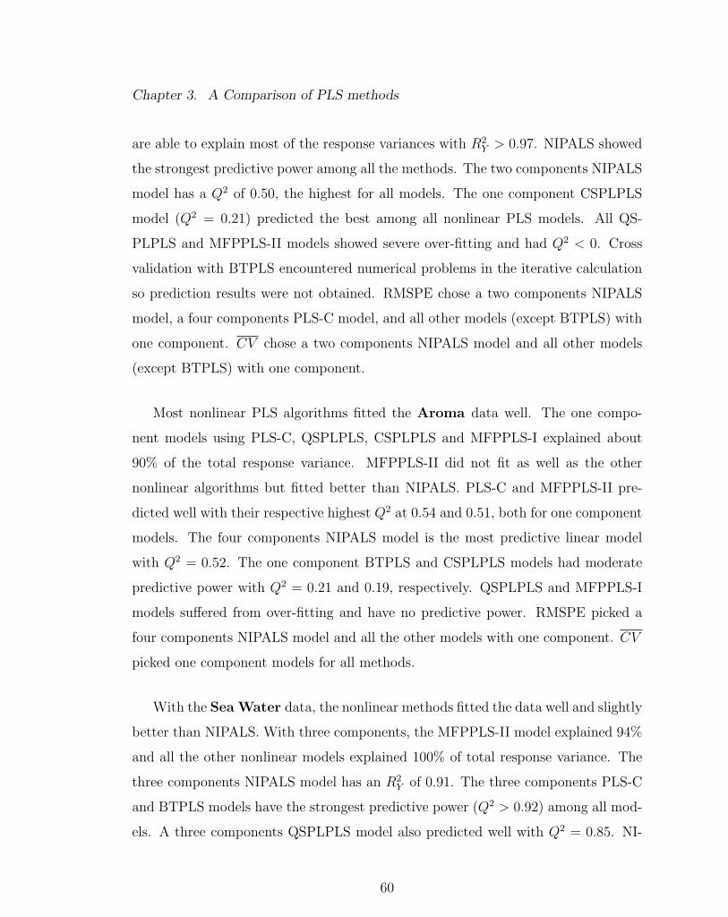
Chapter 3. A Comparison of PLS methods
are able to explain most of the response variances with R2Y > 0.97. NIPALS showed
the strongest predictive power among all the methods. The two components NIPALS
model has a Q2 of 0.50, the highest for all models. The one component CSPLPLS
model (Q2 = 0.21) predicted the best among all nonlinear PLS models. All QS-
PLPLS and MFPPLS-II models showed severe over-fitting and had Q2 < 0. Cross
validation with BTPLS encountered numerical problems in the iterative calculation
so prediction results were not obtained. RMSPE chose a two components NIPALS
model, a four components PLS-C model, and all other models (except BTPLS) with
one component. CV chose a two components NIPALS model and all other models
(except BTPLS) with one component.
Most nonlinear PLS algorithms fitted the Aroma data well. The one compo-
nent models using PLS-C, QSPLPLS, CSPLPLS and MFPPLS-I explained about
90% of the total response variance. MFPPLS-II did not fit as well as the other
nonlinear algorithms but fitted better than NIPALS. PLS-C and MFPPLS-II pre-
dicted well with their respective highest Q2 at 0.54 and 0.51, both for one component
models. The four components NIPALS model is the most predictive linear model
with Q2 = 0.52. The one component BTPLS and CSPLPLS models had moderate
predictive power with Q2 = 0.21 and 0.19, respectively. QSPLPLS and MFPPLS-I
models suffered from over-fitting and have no predictive power. RMSPE picked a
four components NIPALS model and all the other models with one component. CV
picked one component models for all methods.
With the Sea Water data, the nonlinear methods fitted the data well and slightly
better than NIPALS. With three components, the MFPPLS-II model explained 94%
and all the other nonlinear models explained 100% of total response variance. The
three components NIPALS model has an R2Y of 0.91. The three components PLS-C
and BTPLS models have the strongest predictive power (Q2 > 0.92) among all mod-
els. A three components QSPLPLS model also predicted well with Q2 = 0.85. NI-
60
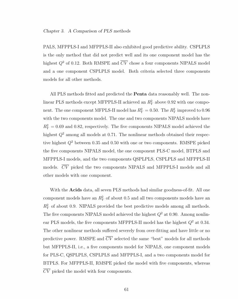
Chapter 3. A Comparison of PLS methods
PALS, MFPPLS-I and MFPPLS-II also exhibited good predictive ability. CSPLPLS
is the only method that did not predict well and its one component model has the
highest Q2 of 0.12. Both RMSPE and CV chose a four components NIPALS model
and a one component CSPLPLS model. Both criteria selected three components
models for all other methods.
All PLS methods fitted and predicted the Penta data reasonably well. The non-
linear PLS methods except MFPPLS-II achieved an R2Y above 0.92 with one compo-
nent. The one component MFPLS-II model has R2Y = 0.50. The R2
Y improved to 0.96
with the two components model. The one and two components NIPALS models have
R2Y = 0.69 and 0.82, respectively. The five components NIPALS model achieved the
highest Q2 among all models at 0.71. The nonlinear methods obtained their respec-
tive highest Q2 between 0.35 and 0.50 with one or two components. RMSPE picked
the five components NIPALS model, the one component PLS-C model, BTPLS and
MFPPLS-I models, and the two components QSPLPLS, CSPLPLS and MFPPLS-II
models. CV picked the two components NIPALS and MFPPLS-I models and all
other models with one component.
With the Acids data, all seven PLS methods had similar goodness-of-fit. All one
component models have an R2Y of about 0.5 and all two components models have an
R2Y of about 0.9. NIPALS provided the best predictive models among all methods.
The five components NIPALS model achieved the highest Q2 at 0.90. Among nonlin-
ear PLS models, the five components MFPPLS-II model has the highest Q2 at 0.34.
The other nonlinear methods suffered severely from over-fitting and have little or no
predictive power. RMSPE and CV selected the same “best” models for all methods
but MFPPLS-II, i.e., a five components model for NIPALS, one component models
for PLS-C, QSPLPLS, CSPLPLS and MFPPLS-I, and a two components model for
BTPLS. For MFPPLS-II, RMSPE picked the model with five components, whereas
CV picked the model with four components.
61
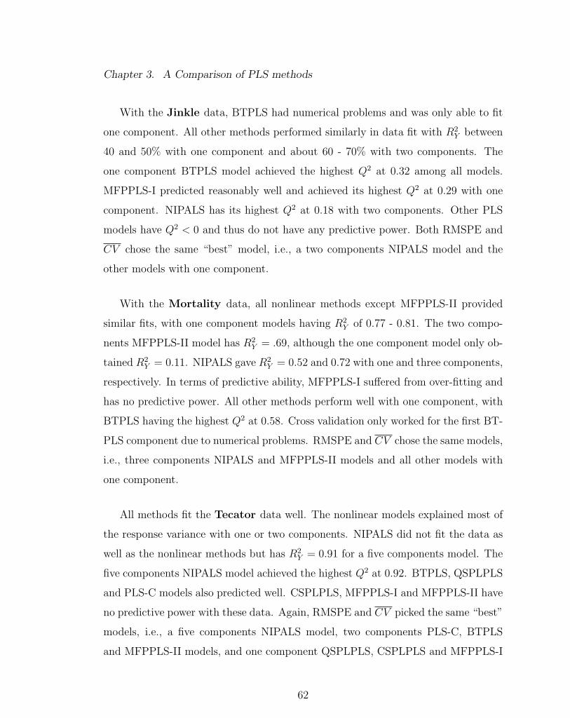
Chapter 3. A Comparison of PLS methods
With the Jinkle data, BTPLS had numerical problems and was only able to fit
one component. All other methods performed similarly in data fit with R2Y between
40 and 50% with one component and about 60 - 70% with two components. The
one component BTPLS model achieved the highest Q2 at 0.32 among all models.
MFPPLS-I predicted reasonably well and achieved its highest Q2 at 0.29 with one
component. NIPALS has its highest Q2 at 0.18 with two components. Other PLS
models have Q2 < 0 and thus do not have any predictive power. Both RMSPE and
CV chose the same “best” model, i.e., a two components NIPALS model and the
other models with one component.
With the Mortality data, all nonlinear methods except MFPPLS-II provided
similar fits, with one component models having R2Y of 0.77 - 0.81. The two compo-
nents MFPPLS-II model has R2Y = .69, although the one component model only ob-
tained R2Y = 0.11. NIPALS gave R2
Y = 0.52 and 0.72 with one and three components,
respectively. In terms of predictive ability, MFPPLS-I suffered from over-fitting and
has no predictive power. All other methods perform well with one component, with
BTPLS having the highest Q2 at 0.58. Cross validation only worked for the first BT-
PLS component due to numerical problems. RMSPE and CV chose the same models,
i.e., three components NIPALS and MFPPLS-II models and all other models with
one component.
All methods fit the Tecator data well. The nonlinear models explained most of
the response variance with one or two components. NIPALS did not fit the data as
well as the nonlinear methods but has R2Y = 0.91 for a five components model. The
five components NIPALS model achieved the highest Q2 at 0.92. BTPLS, QSPLPLS
and PLS-C models also predicted well. CSPLPLS, MFPPLS-I and MFPPLS-II have
no predictive power with these data. Again, RMSPE and CV picked the same “best”
models, i.e., a five components NIPALS model, two components PLS-C, BTPLS
and MFPPLS-II models, and one component QSPLPLS, CSPLPLS and MFPPLS-I
62
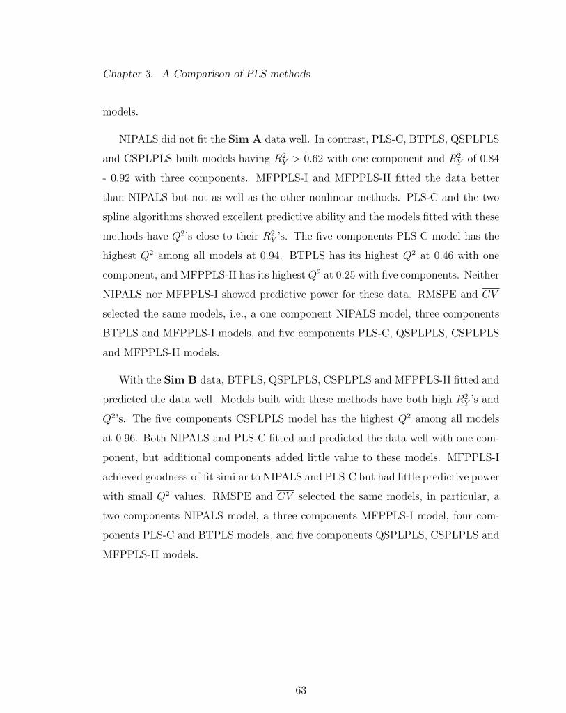
Chapter 3. A Comparison of PLS methods
models.
NIPALS did not fit the Sim A data well. In contrast, PLS-C, BTPLS, QSPLPLS
and CSPLPLS built models having R2Y > 0.62 with one component and R2
Y of 0.84
- 0.92 with three components. MFPPLS-I and MFPPLS-II fitted the data better
than NIPALS but not as well as the other nonlinear methods. PLS-C and the two
spline algorithms showed excellent predictive ability and the models fitted with these
methods have Q2’s close to their R2Y ’s. The five components PLS-C model has the
highest Q2 among all models at 0.94. BTPLS has its highest Q2 at 0.46 with one
component, and MFPPLS-II has its highest Q2 at 0.25 with five components. Neither
NIPALS nor MFPPLS-I showed predictive power for these data. RMSPE and CV
selected the same models, i.e., a one component NIPALS model, three components
BTPLS and MFPPLS-I models, and five components PLS-C, QSPLPLS, CSPLPLS
and MFPPLS-II models.
With the Sim B data, BTPLS, QSPLPLS, CSPLPLS and MFPPLS-II fitted and
predicted the data well. Models built with these methods have both high R2Y ’s and
Q2’s. The five components CSPLPLS model has the highest Q2 among all models
at 0.96. Both NIPALS and PLS-C fitted and predicted the data well with one com-
ponent, but additional components added little value to these models. MFPPLS-I
achieved goodness-of-fit similar to NIPALS and PLS-C but had little predictive power
with small Q2 values. RMSPE and CV selected the same models, in particular, a
two components NIPALS model, a three components MFPPLS-I model, four com-
ponents PLS-C and BTPLS models, and five components QSPLPLS, CSPLPLS and
MFPPLS-II models.
63
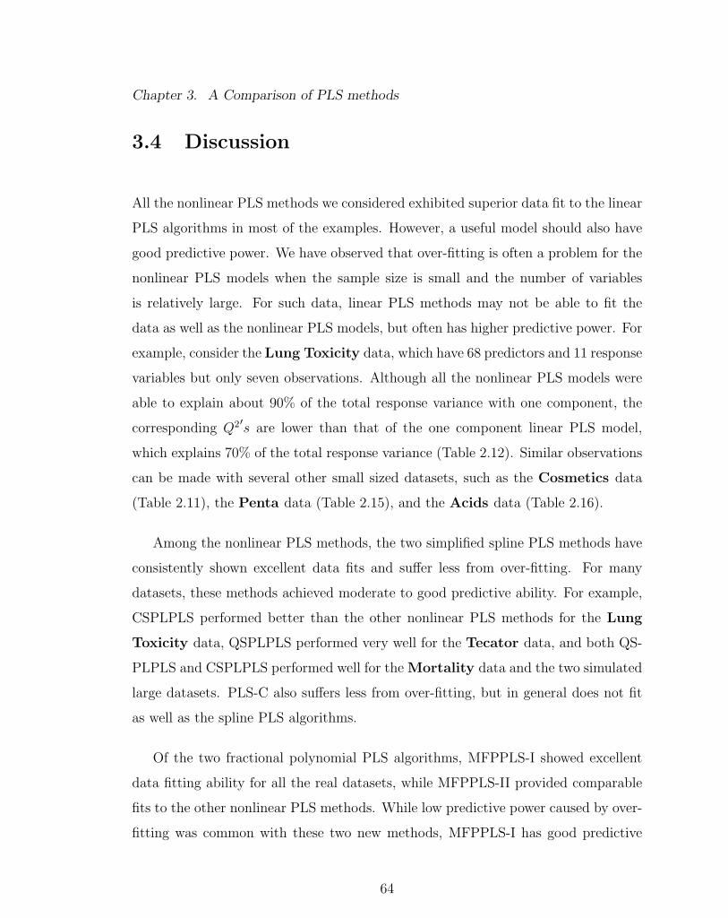
Chapter 3. A Comparison of PLS methods
3.4 Discussion
All the nonlinear PLS methods we considered exhibited superior data fit to the linear
PLS algorithms in most of the examples. However, a useful model should also have
good predictive power. We have observed that over-fitting is often a problem for the
nonlinear PLS models when the sample size is small and the number of variables
is relatively large. For such data, linear PLS methods may not be able to fit the
data as well as the nonlinear PLS models, but often has higher predictive power. For
example, consider the Lung Toxicity data, which have 68 predictors and 11 response
variables but only seven observations. Although all the nonlinear PLS models were
able to explain about 90% of the total response variance with one component, the
corresponding Q2′s are lower than that of the one component linear PLS model,
which explains 70% of the total response variance (Table 2.12). Similar observations
can be made with several other small sized datasets, such as the Cosmetics data
(Table 2.11), the Penta data (Table 2.15), and the Acids data (Table 2.16).
Among the nonlinear PLS methods, the two simplified spline PLS methods have
consistently shown excellent data fits and suffer less from over-fitting. For many
datasets, these methods achieved moderate to good predictive ability. For example,
CSPLPLS performed better than the other nonlinear PLS methods for the Lung
Toxicity data, QSPLPLS performed very well for the Tecator data, and both QS-
PLPLS and CSPLPLS performed well for the Mortality data and the two simulated
large datasets. PLS-C also suffers less from over-fitting, but in general does not fit
as well as the spline PLS algorithms.
Of the two fractional polynomial PLS algorithms, MFPPLS-I showed excellent
data fitting ability for all the real datasets, while MFPPLS-II provided comparable
fits to the other nonlinear PLS methods. While low predictive power caused by over-
fitting was common with these two new methods, MFPPLS-I has good predictive
64
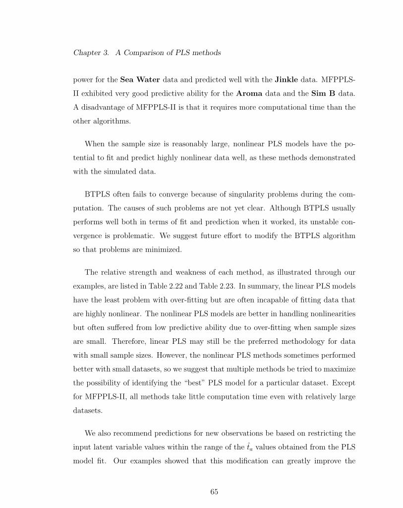
Chapter 3. A Comparison of PLS methods
power for the Sea Water data and predicted well with the Jinkle data. MFPPLS-
II exhibited very good predictive ability for the Aroma data and the Sim B data.
A disadvantage of MFPPLS-II is that it requires more computational time than the
other algorithms.
When the sample size is reasonably large, nonlinear PLS models have the po-
tential to fit and predict highly nonlinear data well, as these methods demonstrated
with the simulated data.
BTPLS often fails to converge because of singularity problems during the com-
putation. The causes of such problems are not yet clear. Although BTPLS usually
performs well both in terms of fit and prediction when it worked, its unstable con-
vergence is problematic. We suggest future effort to modify the BTPLS algorithm
so that problems are minimized.
The relative strength and weakness of each method, as illustrated through our
examples, are listed in Table 2.22 and Table 2.23. In summary, the linear PLS models
have the least problem with over-fitting but are often incapable of fitting data that
are highly nonlinear. The nonlinear PLS models are better in handling nonlinearities
but often suffered from low predictive ability due to over-fitting when sample sizes
are small. Therefore, linear PLS may still be the preferred methodology for data
with small sample sizes. However, the nonlinear PLS methods sometimes performed
better with small datasets, so we suggest that multiple methods be tried to maximize
the possibility of identifying the “best” PLS model for a particular dataset. Except
for MFPPLS-II, all methods take little computation time even with relatively large
datasets.
We also recommend predictions for new observations be based on restricting the
input latent variable values within the range of the ta values obtained from the PLS
model fit. Our examples showed that this modification can greatly improve the
65

Chapter 3. A Comparison of PLS methods
prediction accuracy, especially with the nonlinear PLS models.
66
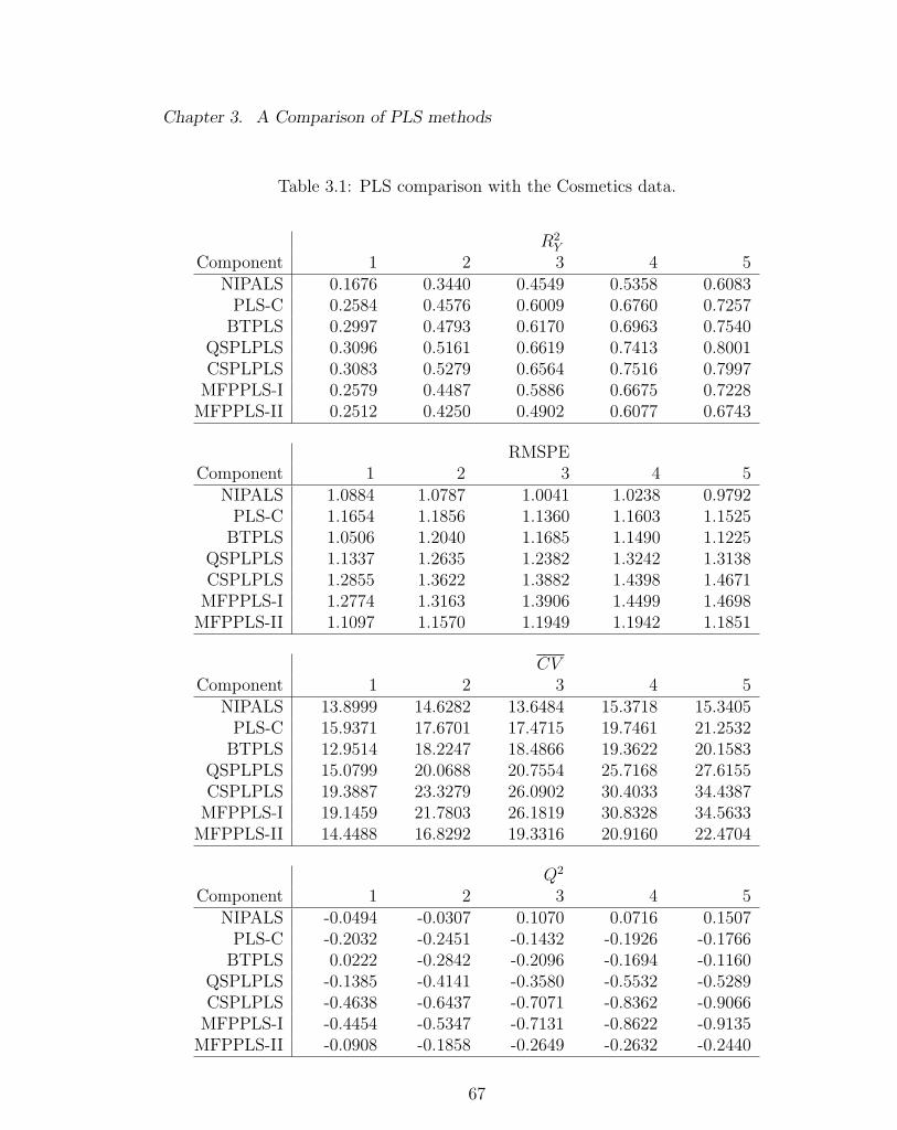
Chapter 3. A Comparison of PLS methods
Table 3.1: PLS comparison with the Cosmetics data.
R2Y
Component 1 2 3 4 5NIPALS 0.1676 0.3440 0.4549 0.5358 0.6083
PLS-C 0.2584 0.4576 0.6009 0.6760 0.7257BTPLS 0.2997 0.4793 0.6170 0.6963 0.7540
QSPLPLS 0.3096 0.5161 0.6619 0.7413 0.8001CSPLPLS 0.3083 0.5279 0.6564 0.7516 0.7997
MFPPLS-I 0.2579 0.4487 0.5886 0.6675 0.7228MFPPLS-II 0.2512 0.4250 0.4902 0.6077 0.6743
RMSPEComponent 1 2 3 4 5
NIPALS 1.0884 1.0787 1.0041 1.0238 0.9792PLS-C 1.1654 1.1856 1.1360 1.1603 1.1525
BTPLS 1.0506 1.2040 1.1685 1.1490 1.1225QSPLPLS 1.1337 1.2635 1.2382 1.3242 1.3138CSPLPLS 1.2855 1.3622 1.3882 1.4398 1.4671
MFPPLS-I 1.2774 1.3163 1.3906 1.4499 1.4698MFPPLS-II 1.1097 1.1570 1.1949 1.1942 1.1851
CVComponent 1 2 3 4 5
NIPALS 13.8999 14.6282 13.6484 15.3718 15.3405PLS-C 15.9371 17.6701 17.4715 19.7461 21.2532
BTPLS 12.9514 18.2247 18.4866 19.3622 20.1583QSPLPLS 15.0799 20.0688 20.7554 25.7168 27.6155CSPLPLS 19.3887 23.3279 26.0902 30.4033 34.4387
MFPPLS-I 19.1459 21.7803 26.1819 30.8328 34.5633MFPPLS-II 14.4488 16.8292 19.3316 20.9160 22.4704
Q2
Component 1 2 3 4 5NIPALS -0.0494 -0.0307 0.1070 0.0716 0.1507
PLS-C -0.2032 -0.2451 -0.1432 -0.1926 -0.1766BTPLS 0.0222 -0.2842 -0.2096 -0.1694 -0.1160
QSPLPLS -0.1385 -0.4141 -0.3580 -0.5532 -0.5289CSPLPLS -0.4638 -0.6437 -0.7071 -0.8362 -0.9066
MFPPLS-I -0.4454 -0.5347 -0.7131 -0.8622 -0.9135MFPPLS-II -0.0908 -0.1858 -0.2649 -0.2632 -0.2440
67
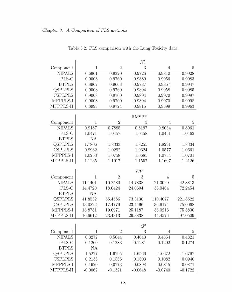
Chapter 3. A Comparison of PLS methods
Table 3.2: PLS comparison with the Lung Toxicity data.
R2Y
Component 1 2 3 4 5NIPALS 0.6961 0.9320 0.9726 0.9810 0.9928
PLS-C 0.9008 0.9760 0.9889 0.9956 0.9983BTPLS 0.8962 0.9663 0.9787 0.9857 0.9947
QSPLPLS 0.9008 0.9760 0.9894 0.9958 0.9985CSPLPLS 0.9008 0.9760 0.9894 0.9970 0.9997
MFPPLS-I 0.9008 0.9760 0.9894 0.9970 0.9998MFPPLS-II 0.8998 0.9724 0.9815 0.9899 0.9963
RMSPEComponent 1 2 3 4 5
NIPALS 0.9187 0.7885 0.8197 0.8034 0.8061PLS-C 1.0471 1.0457 1.0458 1.0451 1.0462
BTPLS NAQSPLPLS 1.7806 1.8333 1.8255 1.8291 1.8334CSPLPLS 0.9932 1.0292 1.0324 1.0577 1.0661
MFPPLS-I 1.0253 1.0758 1.0685 1.0734 1.0701MFPPLS-II 1.1235 1.1917 1.1557 1.1607 1.2126
CVComponent 1 2 3 4 5
NIPALS 11.1401 10.2580 14.7838 21.3020 42.8813PLS-C 14.4720 18.0424 24.0604 36.0464 72.2454
BTPLS NAQSPLPLS 41.8532 55.4586 73.3130 110.4077 221.8522CSPLPLS 13.0222 17.4779 23.4496 36.9174 75.0068
MFPPLS-I 13.8751 19.0971 25.1187 38.0216 75.5800MFPPLS-II 16.6612 23.4313 29.3838 44.4576 97.0509
Q2
Component 1 2 3 4 5NIPALS 0.3272 0.5044 0.4643 0.4854 0.4821
PLS-C 0.1260 0.1283 0.1281 0.1292 0.1274BTPLS NA
QSPLPLS -1.5277 -1.6795 -1.6566 -1.6672 -1.6797CSPLPLS 0.2135 0.1556 0.1503 0.1082 0.0940
MFPPLS-I 0.1620 0.0773 0.0898 0.0815 0.0871MFPPLS-II -0.0062 -0.1321 -0.0648 -0.0740 -0.1722
68
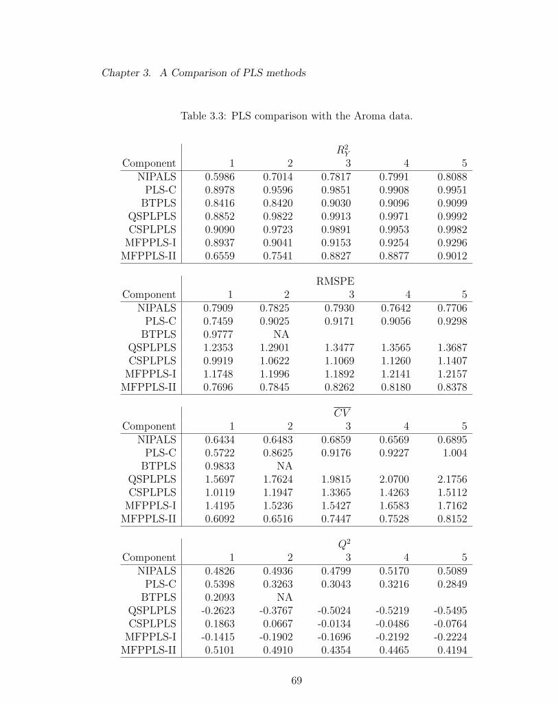
Chapter 3. A Comparison of PLS methods
Table 3.3: PLS comparison with the Aroma data.
R2Y
Component 1 2 3 4 5NIPALS 0.5986 0.7014 0.7817 0.7991 0.8088
PLS-C 0.8978 0.9596 0.9851 0.9908 0.9951BTPLS 0.8416 0.8420 0.9030 0.9096 0.9099
QSPLPLS 0.8852 0.9822 0.9913 0.9971 0.9992CSPLPLS 0.9090 0.9723 0.9891 0.9953 0.9982
MFPPLS-I 0.8937 0.9041 0.9153 0.9254 0.9296MFPPLS-II 0.6559 0.7541 0.8827 0.8877 0.9012
RMSPEComponent 1 2 3 4 5
NIPALS 0.7909 0.7825 0.7930 0.7642 0.7706PLS-C 0.7459 0.9025 0.9171 0.9056 0.9298
BTPLS 0.9777 NAQSPLPLS 1.2353 1.2901 1.3477 1.3565 1.3687CSPLPLS 0.9919 1.0622 1.1069 1.1260 1.1407
MFPPLS-I 1.1748 1.1996 1.1892 1.2141 1.2157MFPPLS-II 0.7696 0.7845 0.8262 0.8180 0.8378
CVComponent 1 2 3 4 5
NIPALS 0.6434 0.6483 0.6859 0.6569 0.6895PLS-C 0.5722 0.8625 0.9176 0.9227 1.004
BTPLS 0.9833 NAQSPLPLS 1.5697 1.7624 1.9815 2.0700 2.1756CSPLPLS 1.0119 1.1947 1.3365 1.4263 1.5112
MFPPLS-I 1.4195 1.5236 1.5427 1.6583 1.7162MFPPLS-II 0.6092 0.6516 0.7447 0.7528 0.8152
Q2
Component 1 2 3 4 5NIPALS 0.4826 0.4936 0.4799 0.5170 0.5089
PLS-C 0.5398 0.3263 0.3043 0.3216 0.2849BTPLS 0.2093 NA
QSPLPLS -0.2623 -0.3767 -0.5024 -0.5219 -0.5495CSPLPLS 0.1863 0.0667 -0.0134 -0.0486 -0.0764
MFPPLS-I -0.1415 -0.1902 -0.1696 -0.2192 -0.2224MFPPLS-II 0.5101 0.4910 0.4354 0.4465 0.4194
69
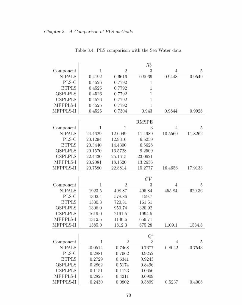
Chapter 3. A Comparison of PLS methods
Table 3.4: PLS comparison with the Sea Water data.
R2Y
Component 1 2 3 4 5NIPALS 0.4192 0.6616 0.9069 0.9448 0.9549
PLS-C 0.4526 0.7792 1BTPLS 0.4525 0.7792 1
QSPLPLS 0.4526 0.7792 1CSPLPLS 0.4526 0.7792 1
MFPPLS-I 0.4526 0.7792 1MFPPLS-II 0.4525 0.7304 0.943 0.9844 0.9928
RMSPEComponent 1 2 3 4 5
NIPALS 24.4629 12.0049 11.4989 10.5560 11.8262PLS-C 20.1294 12.9316 6.5259
BTPLS 20.3440 14.4300 6.5628QSPLPLS 20.1570 16.5728 9.2509CSPLPLS 22.4430 25.1615 23.0621
MFPPLS-I 20.2081 18.1520 13.2636MFPPLS-II 20.7580 22.8814 15.2777 16.4656 17.9133
CVComponent 1 2 3 4 5
NIPALS 1923.5 498.87 495.84 455.84 629.36PLS-C 1302.4 578.86 159.7
BTPLS 1330.3 720.81 161.51QSPLPLS 1306.0 950.74 320.92CSPLPLS 1619.0 2191.5 1994.5
MFPPLS-I 1312.6 1140.6 659.71MFPPLS-II 1385.0 1812.3 875.28 1109.1 1534.8
Q2
Component 1 2 3 4 5NIPALS -0.0514 0.7468 0.7677 0.8042 0.7543
PLS-C 0.2881 0.7062 0.9252BTPLS 0.2729 0.6341 0.9243
QSPLPLS 0.2862 0.5174 0.8496CSPLPLS 0.1151 -0.1123 0.0656
MFPPLS-I 0.2825 0.4211 0.6909MFPPLS-II 0.2430 0.0802 0.5899 0.5237 0.4008
70
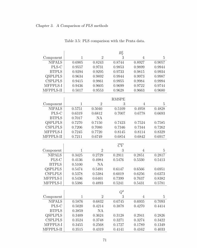
Chapter 3. A Comparison of PLS methods
Table 3.5: PLS comparison with the Penta data.
R2Y
Component 1 2 3 4 5NIPALS 0.6905 0.8243 0.8744 0.8927 0.9057
PLS-C 0.9557 0.9731 0.9853 0.9899 0.9944BTPLS 0.9294 0.9295 0.9733 0.9815 0.9934
QSPLPLS 0.9634 0.9892 0.9944 0.9973 0.9987CSPLPLS 0.9415 0.9861 0.9955 0.9984 0.9994
MFPPLS-I 0.9436 0.9605 0.9699 0.9722 0.9744MFPPLS-II 0.5017 0.9553 0.9628 0.9663 0.9680
RMSPEComponent 1 2 3 4 5
NIPALS 0.5751 0.5040 0.5109 0.4958 0.4828PLS-C 0.6319 0.6812 0.7007 0.6778 0.6693
BTPLS 0.7017 NAQSPLPLS 0.7270 0.7150 0.7423 0.7524 0.7585CSPLPLS 0.7206 0.7080 0.7346 0.7344 0.7262
MFPPLS-I 0.7245 0.7720 0.8145 0.8114 0.8329MFPPLS-II 0.7211 0.6749 0.6854 0.6842 0.6917
CVComponent 1 2 3 4 5
NIPALS 0.3425 0.2729 0.2911 0.2851 0.2817PLS-C 0.4136 0.4984 0.5476 0.5330 0.5413
BTPLS 0.5100 NAQSPLPLS 0.5474 0.5491 0.6147 0.6566 0.6951CSPLPLS 0.5378 0.5384 0.6019 0.6256 0.6373
MFPPLS-I 0.5436 0.6401 0.7399 0.7637 0.8382MFPPLS-I 0.5386 0.4893 0.5241 0.5431 0.5781
Q2
Component 1 2 3 4 5NIPALS 0.5876 0.6832 0.6745 0.6935 0.7093
PLS-C 0.5020 0.4214 0.3878 0.4270 0.4414BTPLS 0.3859 NA
QSPLPLS 0.3409 0.3624 0.3128 0.2941 0.2826CSPLPLS 0.3524 0.3748 0.3271 0.3274 0.3422
MFPPLS-I 0.3455 0.2568 0.1727 0.1789 0.1349MFPPLS-II 0.3515 0.4319 0.4141 0.4162 0.4033
71
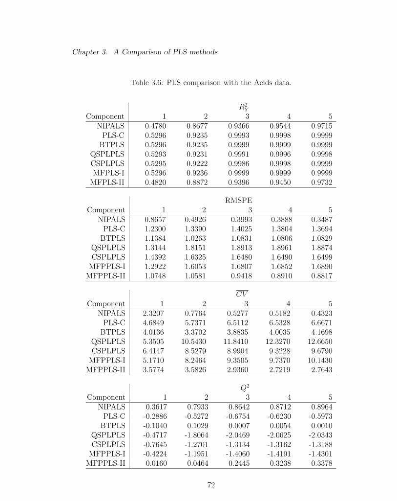
Chapter 3. A Comparison of PLS methods
Table 3.6: PLS comparison with the Acids data.
R2Y
Component 1 2 3 4 5NIPALS 0.4780 0.8677 0.9366 0.9544 0.9715
PLS-C 0.5296 0.9235 0.9993 0.9998 0.9999BTPLS 0.5296 0.9235 0.9999 0.9999 0.9999
QSPLPLS 0.5293 0.9231 0.9991 0.9996 0.9998CSPLPLS 0.5295 0.9222 0.9986 0.9998 0.9999MFPLS-I 0.5296 0.9236 0.9999 0.9999 0.9999
MFPLS-II 0.4820 0.8872 0.9396 0.9450 0.9732
RMSPEComponent 1 2 3 4 5
NIPALS 0.8657 0.4926 0.3993 0.3888 0.3487PLS-C 1.2300 1.3390 1.4025 1.3804 1.3694
BTPLS 1.1384 1.0263 1.0831 1.0806 1.0829QSPLPLS 1.3144 1.8151 1.8913 1.8961 1.8874CSPLPLS 1.4392 1.6325 1.6480 1.6490 1.6499
MFPPLS-I 1.2922 1.6053 1.6807 1.6852 1.6890MFPPLS-II 1.0748 1.0581 0.9418 0.8910 0.8817
CVComponent 1 2 3 4 5
NIPALS 2.3207 0.7764 0.5277 0.5182 0.4323PLS-C 4.6849 5.7371 6.5112 6.5328 6.6671
BTPLS 4.0136 3.3702 3.8835 4.0035 4.1698QSPLPLS 5.3505 10.5430 11.8410 12.3270 12.6650CSPLPLS 6.4147 8.5279 8.9904 9.3228 9.6790
MFPPLS-I 5.1710 8.2464 9.3505 9.7370 10.1430MFPPLS-II 3.5774 3.5826 2.9360 2.7219 2.7643
Q2
Component 1 2 3 4 5NIPALS 0.3617 0.7933 0.8642 0.8712 0.8964
PLS-C -0.2886 -0.5272 -0.6754 -0.6230 -0.5973BTPLS -0.1040 0.1029 0.0007 0.0054 0.0010
QSPLPLS -0.4717 -1.8064 -2.0469 -2.0625 -2.0343CSPLPLS -0.7645 -1.2701 -1.3134 -1.3162 -1.3188
MFPPLS-I -0.4224 -1.1951 -1.4060 -1.4191 -1.4301MFPPLS-II 0.0160 0.0464 0.2445 0.3238 0.3378
72
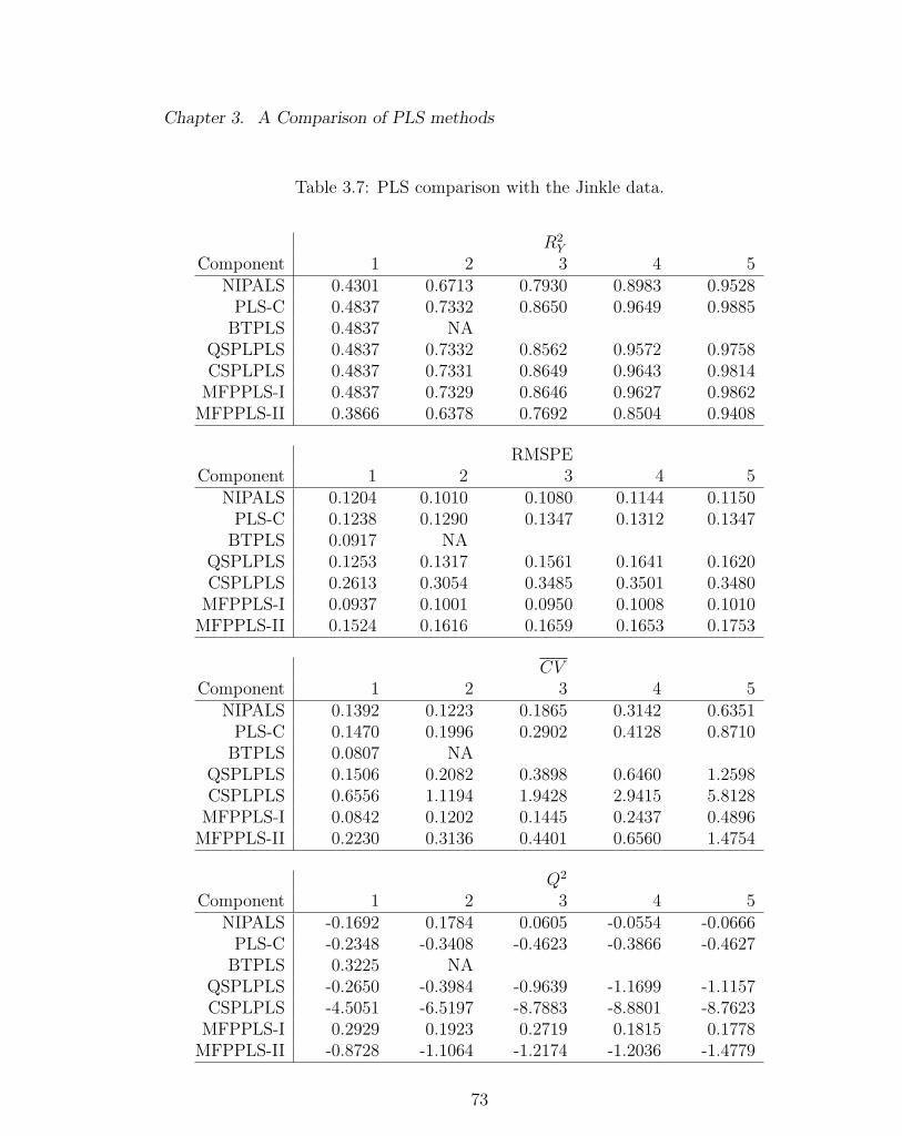
Chapter 3. A Comparison of PLS methods
Table 3.7: PLS comparison with the Jinkle data.
R2Y
Component 1 2 3 4 5NIPALS 0.4301 0.6713 0.7930 0.8983 0.9528
PLS-C 0.4837 0.7332 0.8650 0.9649 0.9885BTPLS 0.4837 NA
QSPLPLS 0.4837 0.7332 0.8562 0.9572 0.9758CSPLPLS 0.4837 0.7331 0.8649 0.9643 0.9814
MFPPLS-I 0.4837 0.7329 0.8646 0.9627 0.9862MFPPLS-II 0.3866 0.6378 0.7692 0.8504 0.9408
RMSPEComponent 1 2 3 4 5
NIPALS 0.1204 0.1010 0.1080 0.1144 0.1150PLS-C 0.1238 0.1290 0.1347 0.1312 0.1347
BTPLS 0.0917 NAQSPLPLS 0.1253 0.1317 0.1561 0.1641 0.1620CSPLPLS 0.2613 0.3054 0.3485 0.3501 0.3480
MFPPLS-I 0.0937 0.1001 0.0950 0.1008 0.1010MFPPLS-II 0.1524 0.1616 0.1659 0.1653 0.1753
CVComponent 1 2 3 4 5
NIPALS 0.1392 0.1223 0.1865 0.3142 0.6351PLS-C 0.1470 0.1996 0.2902 0.4128 0.8710
BTPLS 0.0807 NAQSPLPLS 0.1506 0.2082 0.3898 0.6460 1.2598CSPLPLS 0.6556 1.1194 1.9428 2.9415 5.8128
MFPPLS-I 0.0842 0.1202 0.1445 0.2437 0.4896MFPPLS-II 0.2230 0.3136 0.4401 0.6560 1.4754
Q2
Component 1 2 3 4 5NIPALS -0.1692 0.1784 0.0605 -0.0554 -0.0666
PLS-C -0.2348 -0.3408 -0.4623 -0.3866 -0.4627BTPLS 0.3225 NA
QSPLPLS -0.2650 -0.3984 -0.9639 -1.1699 -1.1157CSPLPLS -4.5051 -6.5197 -8.7883 -8.8801 -8.7623
MFPPLS-I 0.2929 0.1923 0.2719 0.1815 0.1778MFPPLS-II -0.8728 -1.1064 -1.2174 -1.2036 -1.4779
73
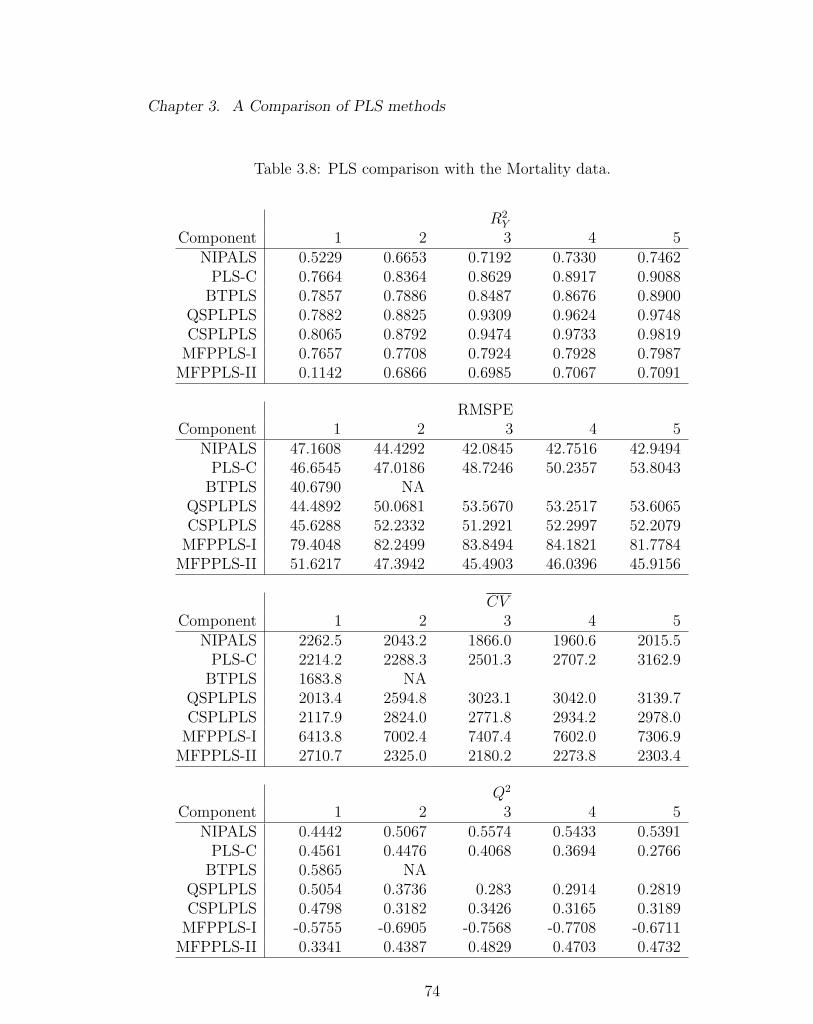
Chapter 3. A Comparison of PLS methods
Table 3.8: PLS comparison with the Mortality data.
R2Y
Component 1 2 3 4 5NIPALS 0.5229 0.6653 0.7192 0.7330 0.7462
PLS-C 0.7664 0.8364 0.8629 0.8917 0.9088BTPLS 0.7857 0.7886 0.8487 0.8676 0.8900
QSPLPLS 0.7882 0.8825 0.9309 0.9624 0.9748CSPLPLS 0.8065 0.8792 0.9474 0.9733 0.9819
MFPPLS-I 0.7657 0.7708 0.7924 0.7928 0.7987MFPPLS-II 0.1142 0.6866 0.6985 0.7067 0.7091
RMSPEComponent 1 2 3 4 5
NIPALS 47.1608 44.4292 42.0845 42.7516 42.9494PLS-C 46.6545 47.0186 48.7246 50.2357 53.8043
BTPLS 40.6790 NAQSPLPLS 44.4892 50.0681 53.5670 53.2517 53.6065CSPLPLS 45.6288 52.2332 51.2921 52.2997 52.2079
MFPPLS-I 79.4048 82.2499 83.8494 84.1821 81.7784MFPPLS-II 51.6217 47.3942 45.4903 46.0396 45.9156
CVComponent 1 2 3 4 5
NIPALS 2262.5 2043.2 1866.0 1960.6 2015.5PLS-C 2214.2 2288.3 2501.3 2707.2 3162.9
BTPLS 1683.8 NAQSPLPLS 2013.4 2594.8 3023.1 3042.0 3139.7CSPLPLS 2117.9 2824.0 2771.8 2934.2 2978.0
MFPPLS-I 6413.8 7002.4 7407.4 7602.0 7306.9MFPPLS-II 2710.7 2325.0 2180.2 2273.8 2303.4
Q2
Component 1 2 3 4 5NIPALS 0.4442 0.5067 0.5574 0.5433 0.5391
PLS-C 0.4561 0.4476 0.4068 0.3694 0.2766BTPLS 0.5865 NA
QSPLPLS 0.5054 0.3736 0.283 0.2914 0.2819CSPLPLS 0.4798 0.3182 0.3426 0.3165 0.3189
MFPPLS-I -0.5755 -0.6905 -0.7568 -0.7708 -0.6711MFPPLS-II 0.3341 0.4387 0.4829 0.4703 0.4732
74
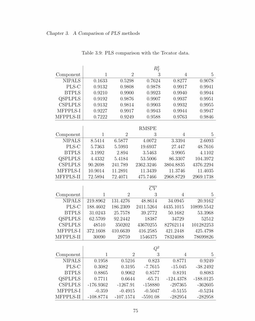
Chapter 3. A Comparison of PLS methods
Table 3.9: PLS comparison with the Tecator data.
R2Y
Component 1 2 3 4 5NIPALS 0.1633 0.5298 0.7624 0.8277 0.9078
PLS-C 0.9132 0.9808 0.9878 0.9917 0.9941BTPLS 0.9210 0.9900 0.9923 0.9940 0.9944
QSPLPLS 0.9192 0.9876 0.9907 0.9937 0.9951CSPLPLS 0.9132 0.9814 0.9903 0.9932 0.9955
MFPPLS-I 0.9227 0.9917 0.9943 0.9944 0.9947MFPPLS-II 0.7222 0.9249 0.9588 0.9763 0.9846
RMSPEComponent 1 2 3 4 5
NIPALS 8.5414 6.5877 4.0072 3.3394 2.6093PLS-C 5.7363 5.5993 19.6937 27.447 48.7616
BTPLS 3.1992 2.894 3.5463 3.9905 4.1102QSPLPLS 4.4332 5.4184 53.5006 86.3307 104.3972CSPLPLS 90.2698 241.789 2362.3246 3804.8835 4376.2294
MFFPLS-I 10.9014 11.2891 11.3439 11.3746 11.4035MFFPLS-II 72.5894 72.4071 475.7466 2968.8729 2969.1738
CVComponent 1 2 3 4 5
NIPALS 219.8962 131.4276 48.8614 34.0945 20.9162PLS-C 188.4602 186.2309 2411.5264 4435.1015 10899.5542
BTPLS 31.0243 25.7578 39.2772 50.1682 53.3968QSPLPLS 62.5709 92.2442 18387 34729 52512CSPLPLS 48510 350202 43670255 82762114 101282253
MFPPLS-I 372.1608 410.6639 416.2585 421.2448 425.4798MFPPLS-II 30090 29759 1546375 78324088 78699826
Q2
Component 1 2 3 4 5NIPALS 0.1958 0.5216 0.823 0.8771 0.9249
PLS-C 0.3082 0.3195 -7.7615 -15.045 -38.2492BTPLS 0.8865 0.9062 0.8577 0.8191 0.8083
QSPLPLS 0.7711 0.6644 -65.71 -124.4378 -188.0125CSPLPLS -176.9362 -1267.91 -158880 -297365 -362605
MFPPLS-I -0.359 -0.4915 -0.5047 -0.5155 -0.5234MFPPLS-II -108.8774 -107.1574 -5591.08 -282954 -282958
75
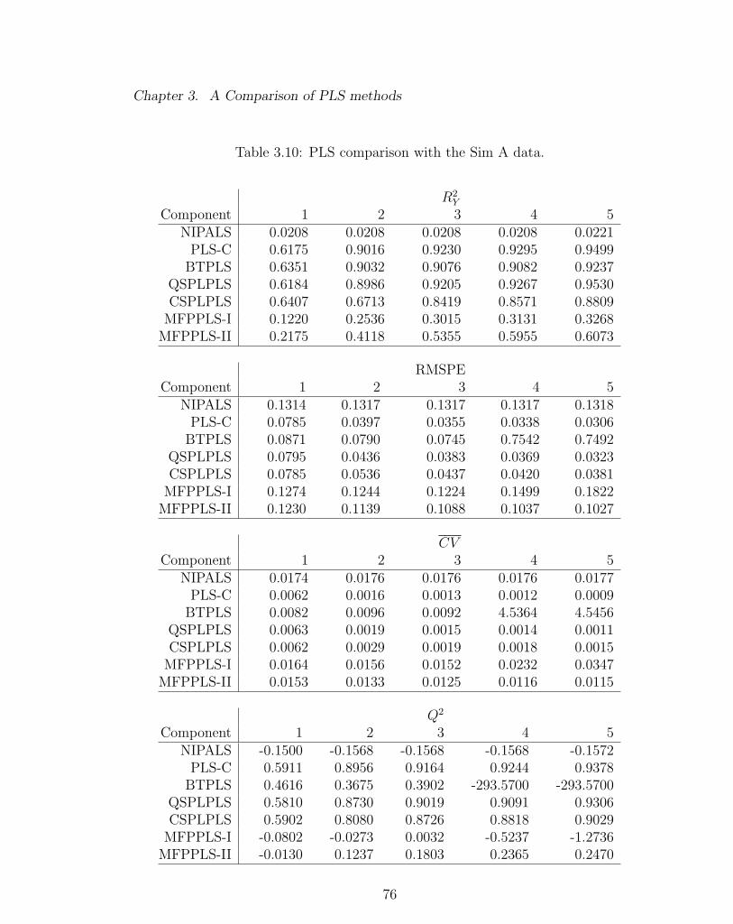
Chapter 3. A Comparison of PLS methods
Table 3.10: PLS comparison with the Sim A data.
R2Y
Component 1 2 3 4 5NIPALS 0.0208 0.0208 0.0208 0.0208 0.0221
PLS-C 0.6175 0.9016 0.9230 0.9295 0.9499BTPLS 0.6351 0.9032 0.9076 0.9082 0.9237
QSPLPLS 0.6184 0.8986 0.9205 0.9267 0.9530CSPLPLS 0.6407 0.6713 0.8419 0.8571 0.8809
MFPPLS-I 0.1220 0.2536 0.3015 0.3131 0.3268MFPPLS-II 0.2175 0.4118 0.5355 0.5955 0.6073
RMSPEComponent 1 2 3 4 5
NIPALS 0.1314 0.1317 0.1317 0.1317 0.1318PLS-C 0.0785 0.0397 0.0355 0.0338 0.0306
BTPLS 0.0871 0.0790 0.0745 0.7542 0.7492QSPLPLS 0.0795 0.0436 0.0383 0.0369 0.0323CSPLPLS 0.0785 0.0536 0.0437 0.0420 0.0381
MFPPLS-I 0.1274 0.1244 0.1224 0.1499 0.1822MFPPLS-II 0.1230 0.1139 0.1088 0.1037 0.1027
CVComponent 1 2 3 4 5
NIPALS 0.0174 0.0176 0.0176 0.0176 0.0177PLS-C 0.0062 0.0016 0.0013 0.0012 0.0009
BTPLS 0.0082 0.0096 0.0092 4.5364 4.5456QSPLPLS 0.0063 0.0019 0.0015 0.0014 0.0011CSPLPLS 0.0062 0.0029 0.0019 0.0018 0.0015
MFPPLS-I 0.0164 0.0156 0.0152 0.0232 0.0347MFPPLS-II 0.0153 0.0133 0.0125 0.0116 0.0115
Q2
Component 1 2 3 4 5NIPALS -0.1500 -0.1568 -0.1568 -0.1568 -0.1572
PLS-C 0.5911 0.8956 0.9164 0.9244 0.9378BTPLS 0.4616 0.3675 0.3902 -293.5700 -293.5700
QSPLPLS 0.5810 0.8730 0.9019 0.9091 0.9306CSPLPLS 0.5902 0.8080 0.8726 0.8818 0.9029
MFPPLS-I -0.0802 -0.0273 0.0032 -0.5237 -1.2736MFPPLS-II -0.0130 0.1237 0.1803 0.2365 0.2470
76
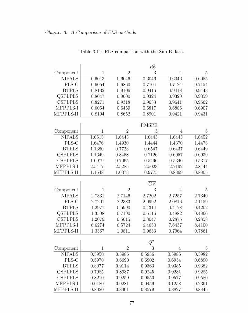
Chapter 3. A Comparison of PLS methods
Table 3.11: PLS comparison with the Sim B data.
R2Y
Component 1 2 3 4 5NIPALS 0.6013 0.6046 0.6046 0.6046 0.6055
PLS-C 0.6054 0.6860 0.7104 0.7124 0.7154BTPLS 0.8132 0.9106 0.9416 0.9418 0.9443
QSPLPLS 0.8047 0.9000 0.9324 0.9329 0.9359CSPLPLS 0.8271 0.9318 0.9633 0.9641 0.9662
MFPPLS-I 0.6054 0.6459 0.6817 0.6886 0.6907MFPPLS-II 0.8194 0.8652 0.8901 0.9421 0.9431
RMSPEComponent 1 2 3 4 5
NIPALS 1.6515 1.6443 1.6443 1.6443 1.6452PLS-C 1.6476 1.4930 1.4444 1.4370 1.4473
BTPLS 1.1380 0.7723 0.6547 0.6437 0.6449QSPLPLS 1.1649 0.8458 0.7126 0.6957 0.6939CSPLPLS 1.0979 0.7065 0.5496 0.5340 0.5317
MFPPLS-I 2.5417 2.5285 2.5023 2.7192 2.8444MFPPLS-II 1.1548 1.0373 0.9775 0.8869 0.8805
CVComponent 1 2 3 4 5
NIPALS 2.7331 2.7146 2.7202 2.7257 2.7340PLS-C 2.7201 2.2383 2.0992 2.0816 2.1159
BTPLS 1.2977 0.5990 0.4314 0.4178 0.4202QSPLPLS 1.3598 0.7190 0.5116 0.4882 0.4866CSPLPLS 1.2079 0.5015 0.3047 0.2876 0.2858
MFPPLS-I 6.6274 6.5724 6.4650 7.6437 8.4100MFPPLS-II 1.3367 1.0811 0.9633 0.7964 0.7861
Q2
Component 1 2 3 4 5NIPALS 0.5950 0.5986 0.5986 0.5986 0.5982
PLS-C 0.5970 0.6690 0.6902 0.6934 0.6890BTPLS 0.8077 0.9114 0.9363 0.9385 0.9382
QSPLPLS 0.7985 0.8937 0.9245 0.9281 0.9285CSPLPLS 0.8210 0.9259 0.9550 0.9577 0.9580
MFPPLS-I 0.0180 0.0281 0.0459 -0.1258 -0.2361MFPPLS-II 0.8020 0.8401 0.8579 0.8827 0.8845
77
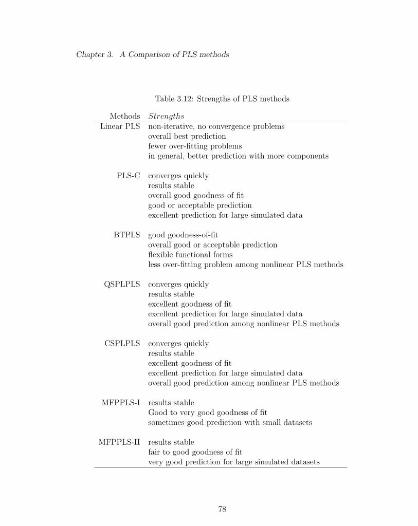
Chapter 3. A Comparison of PLS methods
Table 3.12: Strengths of PLS methods
Methods StrengthsLinear PLS non-iterative, no convergence problems
overall best predictionfewer over-fitting problemsin general, better prediction with more components
PLS-C converges quicklyresults stableoverall good goodness of fitgood or acceptable predictionexcellent prediction for large simulated data
BTPLS good goodness-of-fitoverall good or acceptable predictionflexible functional formsless over-fitting problem among nonlinear PLS methods
QSPLPLS converges quicklyresults stableexcellent goodness of fitexcellent prediction for large simulated dataoverall good prediction among nonlinear PLS methods
CSPLPLS converges quicklyresults stableexcellent goodness of fitexcellent prediction for large simulated dataoverall good prediction among nonlinear PLS methods
MFPPLS-I results stableGood to very good goodness of fitsometimes good prediction with small datasets
MFPPLS-II results stablefair to good goodness of fitvery good prediction for large simulated datasets
78
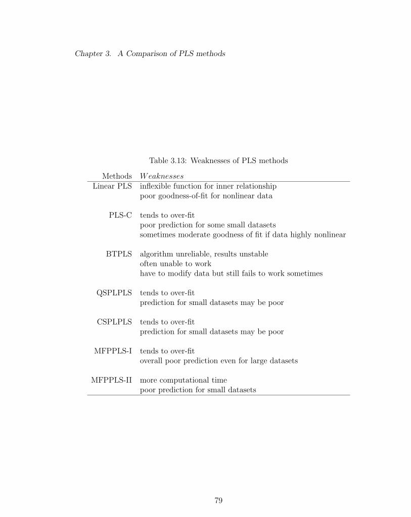
Chapter 3. A Comparison of PLS methods
Table 3.13: Weaknesses of PLS methods
Methods WeaknessesLinear PLS inflexible function for inner relationship
poor goodness-of-fit for nonlinear data
PLS-C tends to over-fitpoor prediction for some small datasetssometimes moderate goodness of fit if data highly nonlinear
BTPLS algorithm unreliable, results unstableoften unable to workhave to modify data but still fails to work sometimes
QSPLPLS tends to over-fitprediction for small datasets may be poor
CSPLPLS tends to over-fitprediction for small datasets may be poor
MFPPLS-I tends to over-fitoverall poor prediction even for large datasets
MFPPLS-II more computational timepoor prediction for small datasets
79
Chapter 4
Supervised Principal Component
Analysis with Multiple Responses
In principal component analysis (PCA), one first decomposes the predictor matrix
X into A principal components ua = Xwa with the first principal component u1
accounting for as much of the variability in X as possible, and each successive com-
ponent accounting for as much of the remaining variability as possible. The compo-
nents also satisfy u1⊥u2⊥...⊥uA. The principal components U can be computed as
follows.
Assume that the columns of XN×P are the mean centered predictor variables.
Write the SVD of X as
X = UDV ′,
where U , D, V are N ×K, K ×K and P ×K respectively, and K = min(N − 1, P )
is the rank of X. D is a diagonal matrix containing the singular values dj with
d1 ≥ d2 ≥ ...dK ≥ 0. The columns of U are the principal components u1, u2, ... ,
uK . From the SVD of X, we also have
80
Chapter 4. Supervised Principal Component Analysis with Multiple Responses
U = XVD−1 = XW ,
where W = V D−1 is the principal component weight matrix.
The first few components, which often contain most of the information in X,
are used as new predictors in a regression analysis with a response Y . PCA is a
commonly used regression tool to deal with multicollinearity of predictors and the
number of predictors being larger than the sample size. A potential weakness of
PCA is that its construction does not consider the relationship between X and Y
and thus the resulting components may not contain much information that is useful
in explaining or predicting Y . Supervised PCA (SPCA) is a modified version of
PCA targeting this weakness that appears to be a promising tool for prediction in
regression problems (Bair et al., 2006; Roberts and Michael, 2006).
4.1 Univariate SPCA
SPCA was first proposed as a semi-supervised regression tool for predicting patient
survival with DNA microarray data (Bair and Tibshirani, 2004). Bair et al. (2006)
provided further details. Several applications (Bair et al., 2006; Roberts and Michael,
2006) demonstrated that SPCA is able to identify the underlying structures that are
relevant to the response and often produces more accurate predictions than PCA.
SPCA is similar to conventional PCA except that the components are constructed
on a subset of the predictors, which are selected based on their association with the
response. Bair et al. (2006) proposed the following SPCA algorithm. Let X be
the mean centered N × P predictor matrix and Y be a vector of the single response
variable. First, the standard regression coefficients for measuring the univariate effect
of the jth predictor on Y are calculated:
81
Chapter 4. Supervised Principal Component Analysis with Multiple Responses
sj =X′jY
‖Xj‖ ,
with a scale estimate σ omitted from the calculation since it is common to all sj′s.
Let Cθ be the collection of indices such that |sj| > θ, where θ is a threshold value
estimated by cross validation. Denote Xθ as the matrix consisting of the columns
of X corresponding to Cθ. Then compute the principal components of the reduced
predictor matrix Xθ using the SVD:
Xθ = UθDθV′θ .
The columns of Uθ, say uθ1, uθ2, ..., uθm, are the supervised principal components
of X. Bair et al. (2006) suggest that the first or the first few supervised principal
components be used to fit a regression model. For example, a simple linear regression
model with the first SPCA component uθ1 can be fitted with:
Y spc,θ = Y + γuθ1.
If wθ1 are the principal component weights for uθ1, then
Y spc,θ = Y +Xθβθ,
where βθ = γwθ1. This approach directly extends to models built from multiple
components.
SPCA is applicable to generalized regression settings such as logistic regression
and Cox proportional hazards models. Bair et al. (2006) suggest that a score statistic
be used in place of the standardized regression coefficients to assess the association
between each predictor and the response, followed by the use of the appropriate
generalized regression at the last step.
82
Chapter 4. Supervised Principal Component Analysis with Multiple Responses
4.2 Multivariate Extension of SPCA
To extend the univariate SPCA to multiple responses, we use likelihood ratio test
(LRT) statistics to evaluate the association of each predictor in X with Y , which is
assumed to be a N ×M matrix. Both X and Y are centered to have zero means.
Assume Y = XjBj + Ej, where Xj is the jth predictor in X, Bj is a 1 ×M vector
and the rows of the error term Ej have a multivariate normal distribution N(0,Σj).
This is a simple linear regression model for each response with no intercepts. Write
Yi as an M × 1 vector by stacking the ith observation for each of the M responses
and denote Xji as the ith observation in Xj. Then the likelihood function is
L(Bj,Σj) = (2π)−N2 |Σj|−
N2 exp[−1
2
N∑i=1
((Yi −B′jXji)′Σ−1
j (Yi −B′jXji))]
= (2π)−N2 |Σj|−
N2 exp[−1
2trace(Σ−1
j (Y −XjBj)′(Y −XjBj))],
which implies
L(Bj, Σj) = (2π)−N2
∣∣∣Σj
∣∣∣−N2
exp[−N2trace(Σ−1
j Σj)]
= (2π)−N2
∣∣∣Σj
∣∣∣−N2
exp(−N2
2),
where Bj = (X ′jXj)−1X ′jY and Σj = Y ′(I−MXj
)Y/N . Here I is the N ×N identity
matrix and MXjis a N × N perpendicular projection operator onto C(Xj), i.e.
Xj(Xj′Xj)
−Xj′. Therefore the LRT statistic testing H0 : Bj = 01×M vs. HA : Bj 6=
01×M is
Λj =L(Bj0, Σj0)
L(Bj, Σj)=
∣∣∣Σj0
∣∣∣−N2
∣∣∣Σj
∣∣∣−N2
=
∣∣∣Σj
∣∣∣N2
∣∣∣Σj0
∣∣∣N2
=
∣∣∣Y ′(I−MXj)Y
N
∣∣∣N2
∣∣Y ′YN
∣∣N2
.
83
Chapter 4. Supervised Principal Component Analysis with Multiple Responses
A smaller Λj value indicates a stronger association between Xj and Y .
Once we obtain the LRT statistic Λj for all Xj′s, we rank the Xj
′s according to
increasing values of the Λj′s, i.e., Λ(1) < Λ(2) < ... < Λ(p). The denominator of Λj is
the same for all j′s and therefore it is irrelevant for the ranking. The remaining steps
are similar to the SPCA for single response. Suppose the final selected subset of X
is Xspc and Uspc contains the corresponding principal components. The prediction
for a new observation Y ~ can be obtained through
Y ~ = Y + UspcΓ,
where Y is the mean response vector and Γ = (Uspc′Uspc)
−Uspc′Y .
Besides the univariate LRT, we also used a forward selection LRT procedure to
rank the predictor variables, as a means to account for correlations among predictors.
A series of stepwise tests may be better than the univariate tests for selecting the
“best” subset of predictors for SPCA. For example, suppose two predictors are highly
associated with the responses and one is a proxy of the other. If one of them is selected
in the subset for principal component construction, including the other in the subset
may add little extra value. With the univariate LRT, it is highly likely that both these
predictors or neither predictor would be selected in the subset. A stepwise procedure,
analogous to that used in multiple regression for automatic model selection, may be
used to avoid redundant predictors from being selected and thus potentially result in
a more parsimonious SPCA model. A forward selection procedure is straightforward
to implement, as described below.
(1) Calculate univariate LTR statistics Λj for all predictors, and rank Xj in terms
of ascending Λj. Denote the ordered predictors X(1), X(2), ..., X(P ).
(2) Calculate LTR statistics Λ∗j for testing the significance of X(1) with each of the
other predictors X(2), ... , X(P ) individually. In particular, let X(1,s) = [X(1) X(s)]
for s = 2, 3, ..., P and define
84
Chapter 4. Supervised Principal Component Analysis with Multiple Responses
Λ∗j =|Σ∗j |
N2
|Σj0|N2
,
where Σ∗j = (Y ′Y − Y ′X(1,s)(X(1,s)′X(1,s))
−X(1,s)′Y )/N . Next, update and relabel the
ranking of the predictors X(2), ... , X(P ) according to Λ∗j . Let X(2,s) =
[X(1) X(2) X(s)] for s = 3, ..., P .
(3) Find the next forward stepwise selected predictor X(3) using the same ap-
proach as in Step (2). Repeat this step until all P predictors are ordered.
The multivariate SPCA algorithm with univariate LRT tests will be called
MSPCA-I. The forward selection algorithm will be identified as MSPCA-II. With
MSPCA-I and MSPCA-II, a prediction model can be built for K predictors and
A components, provided A ≤ K. For a given value of A, the optimal number
of predictors, denoted as Pspc, can be identified by cross validation, following the
presentation in Section 2.4.2. Similarly, prediction measures such as Q2, CV , and
RMSPE can be compared for a fixed number of predictors and a varying number A
of components.
4.3 Examples
MSPCA-I and MSPCA-II were tested with the datasets that were used in Chapter
3 for comparing PLS algorithms. We compared MSPCA-I and MSPCA-II to each
other and to the PLS algorithms in terms of goodness-of-fit (measured by R2Y ) and
predictive ability (measured by Q2). RMSPE and CV were used to determine the
“best” number of components. As with the comparison of PLS algorithms, LOOCV
was used for the small to medium sized real datasets (N ≤ 60), and five-fold cross
validation was used for the large sized (N = 215) Tecator data and the two simulated
datasets Sim A and Sim B (N = 500).
85
Chapter 4. Supervised Principal Component Analysis with Multiple Responses
Results for MSPCA-I and MSPCA-II are presented in Table 4.1 - 4.11 at the end
of this section. The results shown are based on the models with the optimal number
of predictors for each fixed number of components.
With the Cosmetic data, MSPCA-I and MSPCA-II performed similarly and the
R2′s are the same for all models with one to five components. The one component
models, where only one predictor was selected in the SPC predictor subset, are
equivalent to linear regression models. These models’ ability to fit the data is similar
to that of NIPALS but not as good as the nonlinear PLS models. However, the
MSPCA models suffered less from over-fitting than the nonlinear PLS models but
did not predict as well as NIPALS. RMSPE selected a four components MSPCA-I
model and a three components MSPCA-II model both having a Q2 of 0.12. CV
selected one component models with both methods.
Both MSPCA-I and MSPCA-II fitted and predicted the Lung Toxicity data
well. Both five components models obtained an R2Y near 1. RMSPE selected a five
components MSPCA-I model and a three components MSPCA-II model. MSPCA-I
achieved the highest Q2 of 0.49 with five components, whereas the three components
MSPCA-II model obtained its highestQ2 of 0.32. CV selected one component models
for both methods. The performance of these MSPCA models is similar to NIPALS
and better than nonlinear PLS.
The MSPCA methods performed similarly with the Aroma data. Both one
component MSPCA models have R2Y = 0.63 and MSPCA-I achieved its highest R2
Y
at 0.71 with four components whereas MSPCA-II obtained its highest R2Y at 0.77
with five components. However, the second and subsequent components did not
substantially improve prediction. RMSPE selected the five components MSPCA-
I model and the one component MSPCA-II model. CV chose the one component
model for both methods. MSPCA did not fit the Aroma data as well as PLS methods
but predicted better. The one component MSPCA-II model and the five components
86
Chapter 4. Supervised Principal Component Analysis with Multiple Responses
MSPCA-I model achieved their respective highest Q2 at 0.60 and 0.63, whereas the
highest Q2 from the PLS models is 0.54, achieved by the one component PLS-C
model.
With the Sea Water data, both MSPCA methods fitted and predicted the
data well. Their performance is comparable to that of the PLS methods. Both two
components models have R2Y ’s over 0.83. An interesting observation is that MSPCA-
II seems to be able to fit the data as well as MSPCA-I with fewer predictors. For
example, with five components, MSPCA-II has a higher R2Y than MSPCA-I with 20
predictors. The two components MSPCA-II model has the highest R2Y at 0.85 among
all MSPCA models. Both RMSPE and CV selected a three components MSPCA-I
model and a two components MSPCA-II model.
With the Penta data, both MSPCA methods fitted and predicted the data rea-
sonably well. Although they did not fit as well as the nonlinear PLS methods, they
showed less over-fitting and predicted better. Both three components models ex-
plained about 80% of the response variation. Both methods achieved the highest
Q2 at 0.79 with five components. RMSPE selected the five components model for
both methods, whereas CV prefers a one component MSPCA-I model and a two
components MSPCA-II model.
With the Acids data, both MSPCA methods performed well. Although they
did not fit the data as well as the nonlinear PLS methods, neither did they over-
fit the data and thus predicted better. Both methods have R2Y > 0.9 with three
components. MSPCA-II fitted the data as well as or slightly better than MSPCA-I
with fewer predictors, regardless of the number of components. For example, the
three components MSPCA-II model using three predictors has R2Y = 0.94, whereas
the three components MSPCA-I model needed 21 predictors to have R2Y = 0.92. The
five components MSPCA-II model with 5 predictors has the highest Q2 at 0.93 among
all MSPCA models. Both RMSPE and CV chose a four components MSPCA-I model
87
Chapter 4. Supervised Principal Component Analysis with Multiple Responses
and a five components MSPCA-II model.
Both methods fitted and predicted the Jinkle data well. While the MSPCA
methods achieved comparable fit to the PLS methods, they displayed better robust-
ness and predicted considerably better than any of the PLS algorithms. RMSPE
picked four components MSPCA models, while CV selected two components models.
Both methods achieved their best prediction with four components having Q2 = 0.52.
The MSPCA methods fitted and predicted the Mortality data well. Although
they did not fit as well as most of the nonlinear PLS methods, they predicted better.
Both RMSPE and CV made the same choices of models, i.e. a two components
MSPCA-I model and a five components MSPCA-II model, where both achieved
their respective best prediction with Q2 = 0.61 and 0.62. The forward stepwise
predictor screening procedure selected fewer predictors for two to four components
models than the univariate procedure.
MSPCA-I and MSPCA-II fitted the Tecator data well and their prediction ability
is comparable to the best PLS methods, such as NIPALS, BTPLS and QSPLPLS.
The five components MSPCA-II model has the highest Q2 at 0.93 among all MSPCA
and PLS models. Both RMSPE and CV picked a four components MSPCA-I model
and a five components MSPCA-II model. The forward stepwise procedure once again
picked smaller predictor subsets than the univariate selection procedure.
As with NIPALS, MSPCA-I and MSPCA-II had trouble fitting the nonlinear
Sim A data. Since there are only four predictors in the data, no five components
model is fit. None of these models was able to fit and predict the data.
The performance of the MSPCA models with the Sim B resembles that of NI-
PALS. That is, the one component models were able to fit and predict well (both
R2Y ’s and R2
Y ’s are about 0.6). Additional components provided no further value.
The nonlinear PLS methods fitted and predicted these data considerably better.
88
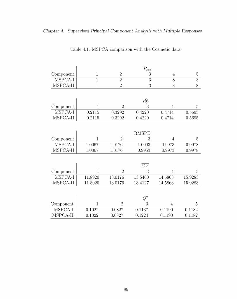
Chapter 4. Supervised Principal Component Analysis with Multiple Responses
Table 4.1: MSPCA comparison with the Cosmetic data.
PspcComponent 1 2 3 4 5
MSPCA-I 1 2 3 8 8MSPCA-II 1 2 3 8 8
R2Y
Component 1 2 3 4 5MSPCA-I 0.2115 0.3292 0.4220 0.4714 0.5695
MSPCA-II 0.2115 0.3292 0.4220 0.4714 0.5695
RMSPEComponent 1 2 3 4 5
MSPCA-I 1.0067 1.0176 1.0003 0.9973 0.9978MSPCA-II 1.0067 1.0176 0.9953 0.9973 0.9978
CVComponent 1 2 3 4 5
MSPCA-I 11.8920 13.0176 13.5460 14.5863 15.9283MSPCA-II 11.8920 13.0176 13.4127 14.5863 15.9283
Q2
Component 1 2 3 4 5MSPCA-I 0.1022 0.0827 0.1137 0.1190 0.1182
MSPCA-II 0.1022 0.0827 0.1224 0.1190 0.1182
89
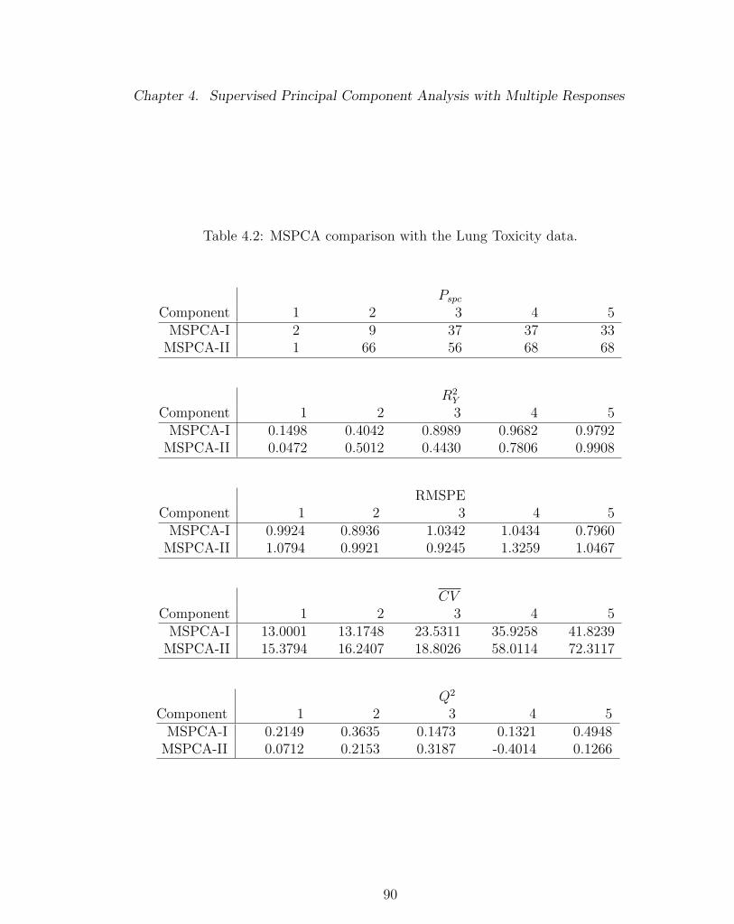
Chapter 4. Supervised Principal Component Analysis with Multiple Responses
Table 4.2: MSPCA comparison with the Lung Toxicity data.
PspcComponent 1 2 3 4 5
MSPCA-I 2 9 37 37 33MSPCA-II 1 66 56 68 68
R2Y
Component 1 2 3 4 5MSPCA-I 0.1498 0.4042 0.8989 0.9682 0.9792
MSPCA-II 0.0472 0.5012 0.4430 0.7806 0.9908
RMSPEComponent 1 2 3 4 5
MSPCA-I 0.9924 0.8936 1.0342 1.0434 0.7960MSPCA-II 1.0794 0.9921 0.9245 1.3259 1.0467
CVComponent 1 2 3 4 5
MSPCA-I 13.0001 13.1748 23.5311 35.9258 41.8239MSPCA-II 15.3794 16.2407 18.8026 58.0114 72.3117
Q2
Component 1 2 3 4 5MSPCA-I 0.2149 0.3635 0.1473 0.1321 0.4948
MSPCA-II 0.0712 0.2153 0.3187 -0.4014 0.1266
90
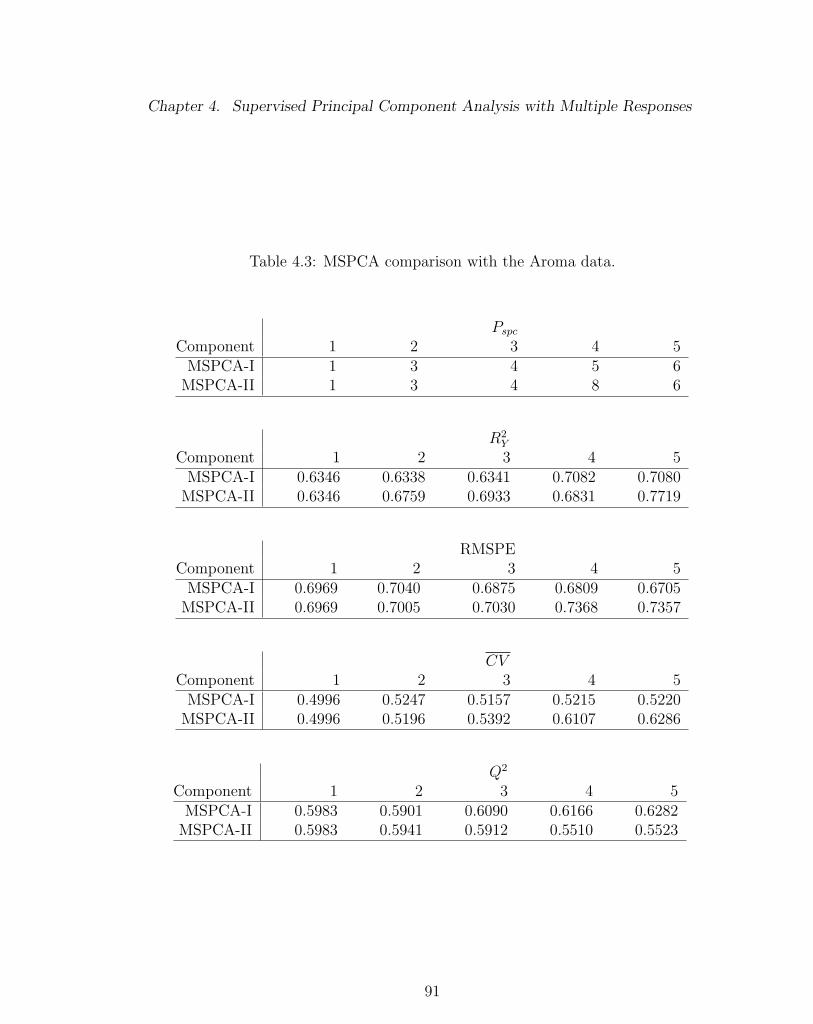
Chapter 4. Supervised Principal Component Analysis with Multiple Responses
Table 4.3: MSPCA comparison with the Aroma data.
PspcComponent 1 2 3 4 5
MSPCA-I 1 3 4 5 6MSPCA-II 1 3 4 8 6
R2Y
Component 1 2 3 4 5MSPCA-I 0.6346 0.6338 0.6341 0.7082 0.7080
MSPCA-II 0.6346 0.6759 0.6933 0.6831 0.7719
RMSPEComponent 1 2 3 4 5
MSPCA-I 0.6969 0.7040 0.6875 0.6809 0.6705MSPCA-II 0.6969 0.7005 0.7030 0.7368 0.7357
CVComponent 1 2 3 4 5
MSPCA-I 0.4996 0.5247 0.5157 0.5215 0.5220MSPCA-II 0.4996 0.5196 0.5392 0.6107 0.6286
Q2
Component 1 2 3 4 5MSPCA-I 0.5983 0.5901 0.6090 0.6166 0.6282
MSPCA-II 0.5983 0.5941 0.5912 0.5510 0.5523
91
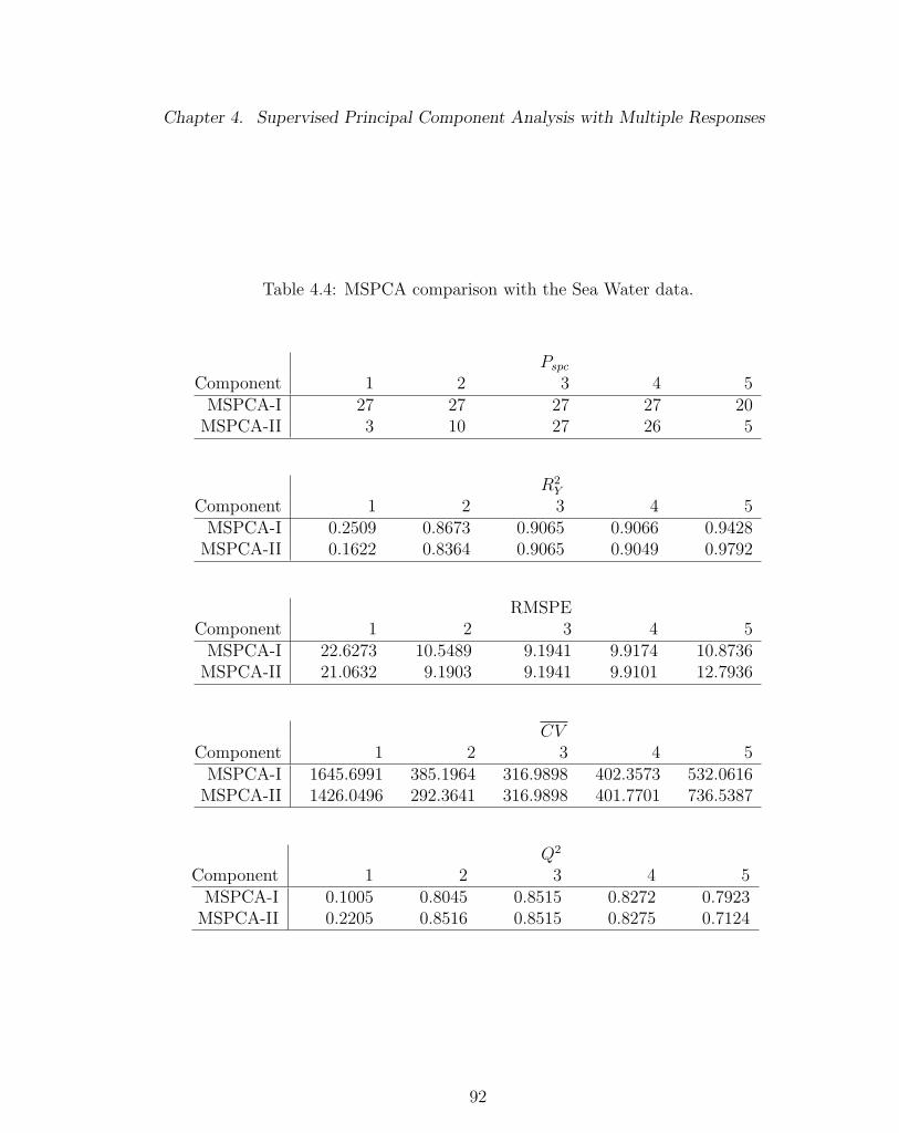
Chapter 4. Supervised Principal Component Analysis with Multiple Responses
Table 4.4: MSPCA comparison with the Sea Water data.
PspcComponent 1 2 3 4 5
MSPCA-I 27 27 27 27 20MSPCA-II 3 10 27 26 5
R2Y
Component 1 2 3 4 5MSPCA-I 0.2509 0.8673 0.9065 0.9066 0.9428
MSPCA-II 0.1622 0.8364 0.9065 0.9049 0.9792
RMSPEComponent 1 2 3 4 5
MSPCA-I 22.6273 10.5489 9.1941 9.9174 10.8736MSPCA-II 21.0632 9.1903 9.1941 9.9101 12.7936
CVComponent 1 2 3 4 5
MSPCA-I 1645.6991 385.1964 316.9898 402.3573 532.0616MSPCA-II 1426.0496 292.3641 316.9898 401.7701 736.5387
Q2
Component 1 2 3 4 5MSPCA-I 0.1005 0.8045 0.8515 0.8272 0.7923
MSPCA-II 0.2205 0.8516 0.8515 0.8275 0.7124
92
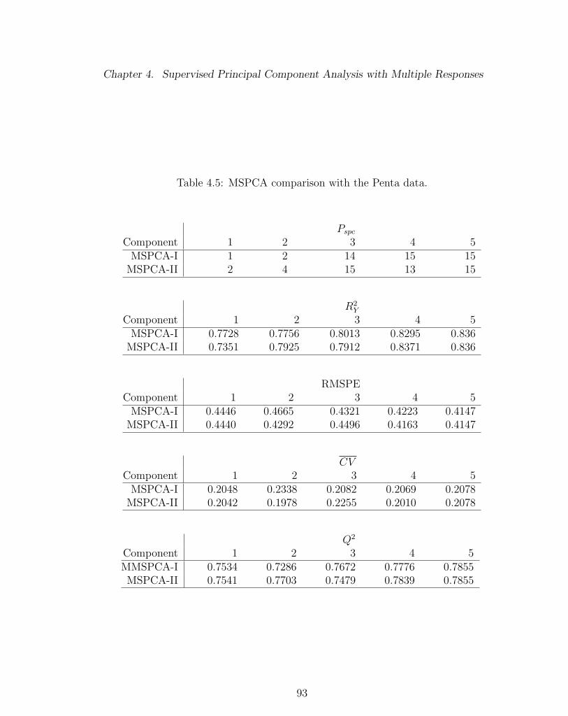
Chapter 4. Supervised Principal Component Analysis with Multiple Responses
Table 4.5: MSPCA comparison with the Penta data.
PspcComponent 1 2 3 4 5
MSPCA-I 1 2 14 15 15MSPCA-II 2 4 15 13 15
R2Y
Component 1 2 3 4 5MSPCA-I 0.7728 0.7756 0.8013 0.8295 0.836
MSPCA-II 0.7351 0.7925 0.7912 0.8371 0.836
RMSPEComponent 1 2 3 4 5
MSPCA-I 0.4446 0.4665 0.4321 0.4223 0.4147MSPCA-II 0.4440 0.4292 0.4496 0.4163 0.4147
CVComponent 1 2 3 4 5
MSPCA-I 0.2048 0.2338 0.2082 0.2069 0.2078MSPCA-II 0.2042 0.1978 0.2255 0.2010 0.2078
Q2
Component 1 2 3 4 5MMSPCA-I 0.7534 0.7286 0.7672 0.7776 0.7855MSPCA-II 0.7541 0.7703 0.7479 0.7839 0.7855
93

Chapter 4. Supervised Principal Component Analysis with Multiple Responses
Table 4.6: MSPCA comparison with the Acids data.
PspcComponent 1 2 3 4 5
MSPCA-I 21 29 21 21 29MSPCA-II 4 9 3 16 6
R2Y
Component 1 2 3 4 5MSPCA-I 0.4335 0.8497 0.9232 0.9343 0.9348
MSPCA-II 0.4271 0.8601 0.9400 0.9346 0.9564
RMSPEComponent 1 2 3 4 5
MSPCA-I 0.8410 0.4588 0.3436 0.3248 0.3286MSPCA-II 0.8210 0.4321 0.3311 0.3276 0.2947
CVComponent 1 2 3 4 5MMSPCA-I 2.1902 0.6737 0.3908 0.3617 0.3840MSPCA-II 2.0872 0.5974 0.3630 0.3680 0.3088
Q2
Component 1 2 3 4 5MSPCA-I 0.3976 0.8207 0.8994 0.9101 0.9080
MSPCA-II 0.4259 0.8410 0.9066 0.9086 0.9260
94

Chapter 4. Supervised Principal Component Analysis with Multiple Responses
Table 4.7: MSPCA comparison with the Jinkle data.
PspcComponent 1 2 3 4 5
MSPCA-I 8 23 24 22 24MSPCA-II 2 24 24 24 24
R2Y
Component 1 2 3 4 5MSPCA-I 0.2529 0.7164 0.869 0.9198 0.9338
MSPCA-II 0.1164 0.7164 0.8690 0.9198 0.9338
RMSPEComponent 1 2 3 4 5
MSPCA-I 0.1070 0.0925 0.0818 0.0772 0.1336MSPCA-II 0.1100 0.0926 0.0818 0.0775 0.1336
CVComponent 1 2 3 4 5
MSPCA-I 0.1098 0.1027 0.1070 0.1429 0.8562MSPCA-II 0.1161 0.1029 0.1070 0.1440 0.8562
Q2
Component 1 2 3 4 5MSPCA-I 0.0776 0.3099 0.4608 0.5201 -0.4379
MSPCA-II 0.0252 0.3086 0.4608 0.5164 -0.4379
95
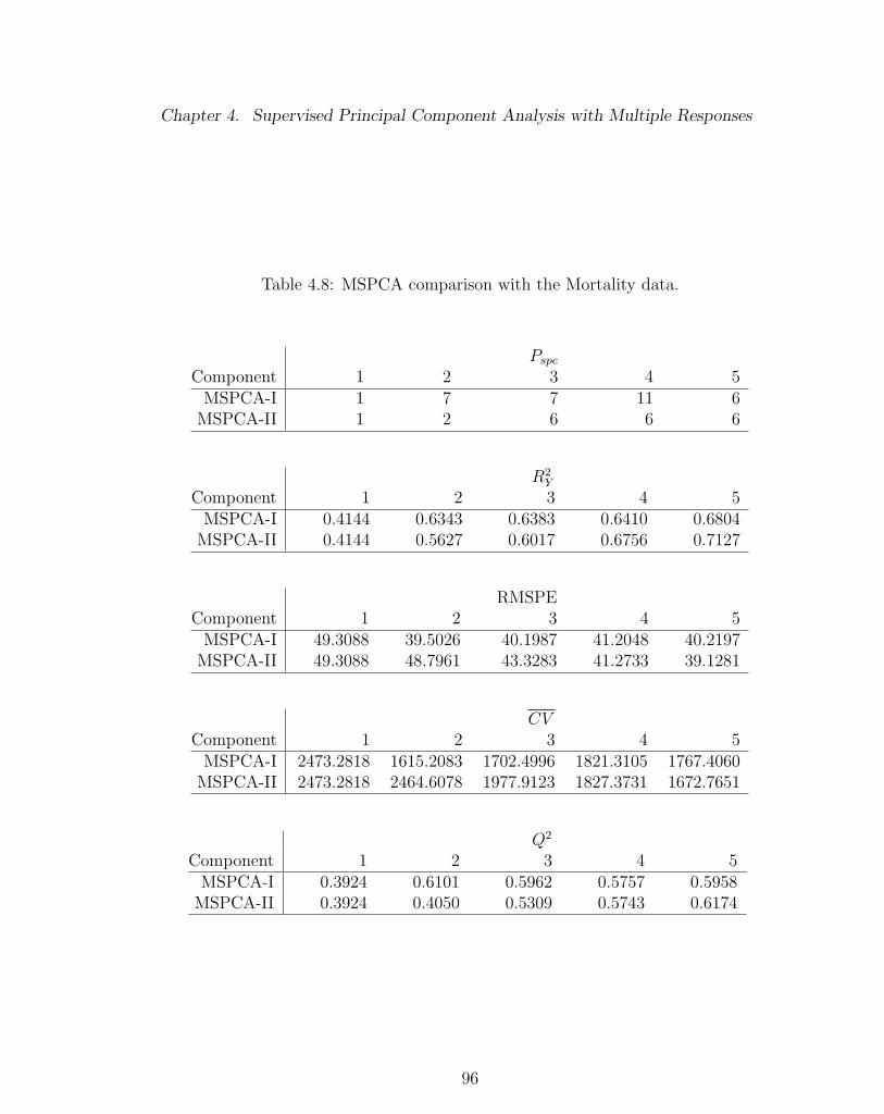
Chapter 4. Supervised Principal Component Analysis with Multiple Responses
Table 4.8: MSPCA comparison with the Mortality data.
PspcComponent 1 2 3 4 5
MSPCA-I 1 7 7 11 6MSPCA-II 1 2 6 6 6
R2Y
Component 1 2 3 4 5MSPCA-I 0.4144 0.6343 0.6383 0.6410 0.6804
MSPCA-II 0.4144 0.5627 0.6017 0.6756 0.7127
RMSPEComponent 1 2 3 4 5
MSPCA-I 49.3088 39.5026 40.1987 41.2048 40.2197MSPCA-II 49.3088 48.7961 43.3283 41.2733 39.1281
CVComponent 1 2 3 4 5
MSPCA-I 2473.2818 1615.2083 1702.4996 1821.3105 1767.4060MSPCA-II 2473.2818 2464.6078 1977.9123 1827.3731 1672.7651
Q2
Component 1 2 3 4 5MSPCA-I 0.3924 0.6101 0.5962 0.5757 0.5958
MSPCA-II 0.3924 0.4050 0.5309 0.5743 0.6174
96
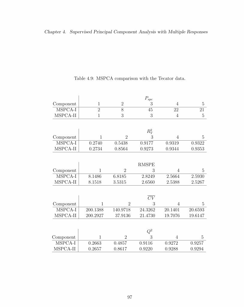
Chapter 4. Supervised Principal Component Analysis with Multiple Responses
Table 4.9: MSPCA comparison with the Tecator data.
PspcComponent 1 2 3 4 5
MSPCA-I 2 8 45 22 21MSPCA-II 1 3 3 4 5
R2Y
Component 1 2 3 4 5MSPCA-I 0.2740 0.5438 0.9177 0.9319 0.9322
MSPCA-II 0.2734 0.8564 0.9273 0.9344 0.9353
RMSPEComponent 1 2 3 4 5
MSPCA-I 8.1486 6.8185 2.8249 2.5664 2.5930MSPCA-II 8.1518 3.5315 2.6560 2.5388 2.5267
CVComponent 1 2 3 4 5
MSPCA-I 200.1388 140.9718 24.3262 20.1401 20.6593MSPCA-II 200.2927 37.9136 21.4730 19.7076 19.6147
Q2
Component 1 2 3 4 5MSPCA-I 0.2663 0.4857 0.9116 0.9272 0.9257
MSPCA-II 0.2657 0.8617 0.9220 0.9288 0.9294
97
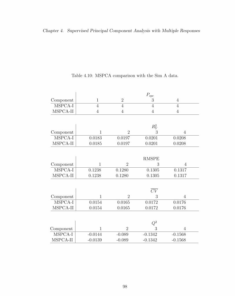
Chapter 4. Supervised Principal Component Analysis with Multiple Responses
Table 4.10: MSPCA comparison with the Sim A data.
PspcComponent 1 2 3 4
MSPCA-I 4 4 4 4MSPCA-II 4 4 4 4
R2Y
Component 1 2 3 4MSPCA-I 0.0183 0.0197 0.0201 0.0208
MSPCA-II 0.0185 0.0197 0.0201 0.0208
RMSPEComponent 1 2 3 4
MSPCA-I 0.1238 0.1280 0.1305 0.1317MSPCA-II 0.1238 0.1280 0.1305 0.1317
CVComponent 1 2 3 4
MSPCA-I 0.0154 0.0165 0.0172 0.0176MSPCA-II 0.0154 0.0165 0.0172 0.0176
Q2
Component 1 2 3 4MSPCA-I -0.0144 -0.089 -0.1342 -0.1568
MSPCA-II -0.0139 -0.089 -0.1342 -0.1568
98
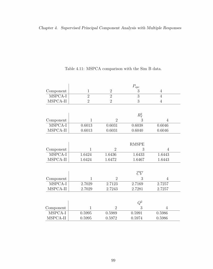
Chapter 4. Supervised Principal Component Analysis with Multiple Responses
Table 4.11: MSPCA comparison with the Sim B data.
PspcComponent 1 2 3 4
MSPCA-I 2 2 3 4MSPCA-II 2 2 3 4
R2Y
Component 1 2 3 4MSPCA-I 0.6013 0.6031 0.6038 0.6046
MSPCA-II 0.6013 0.6031 0.6040 0.6046
RMSPEComponent 1 2 3 4
MSPCA-I 1.6424 1.6436 1.6433 1.6443MSPCA-II 1.6424 1.6472 1.6467 1.6443
CVComponent 1 2 3 4
MSPCA-I 2.7029 2.7123 2.7169 2.7257MSPCA-II 2.7029 2.7243 2.7281 2.7257
Q2
Component 1 2 3 4MSPCA-I 0.5995 0.5989 0.5991 0.5986
MSPCA-II 0.5995 0.5972 0.5974 0.5986
99
Chapter 4. Supervised Principal Component Analysis with Multiple Responses
4.4 Discussion
The comparison between MSPCA-I and MSPCA-II shows that these methods per-
form similarly in both goodness-of-fit and prediction. For most of the real data we
examined, these methods exhibit reasonably good performance. In some cases, al-
though MSPCA methods are not able to fit the data as well as the nonlinear PLS
methods, they are less prone to over-fitting and thus able to predict better. The over-
all performance of these semi-supervised methods resembles that of the linear PLS.
As with the linear PLS, MSPCA is a robust regression tool that can work well with
high dimensional data having severe predictor multicollinearity. However, MSPCA
methods did not fit and predict the two simulated highly nonlinear datasets as well as
the nonlinear PLS methods. Some modifications to the algorithms, such as applying
polynomial transformations to the principal components before the regression, may
potentially improve MSPCA’s performance with such data.
The forward stepwise procedure used in MSPCA-II provided a more effective
means to rank the predictor variables than the univariate procedure in MSPCA-I.
In a number of examples, MSPCA-II selected predictor subsets with fewer variables
yet fitted the data at least as well as MSPCA-I. This was especially true for data
with high predictor multicollinearity, such as the Acids and Tecator data where
MSPCA-II consistently picked fewer predictors than MSPCA-I. MSPCA-II often
provides more parsimonious models and therefore it is preferred to MSPCA-I.
Previous SPCA studies (Bair et al., 2006; Roberts and Michael, 2006) suggested
that the first principal component be used for regression. Our examples show that
more often than not, extra components could add considerable value and result in
more predictive models. We recommend fitting models with a number of components,
say five, and using cross validation to choose the final model.
100
Chapter 5
Conclusion
In Chapter 2, we reviewed the general PLS methodology and two popular linear
PLS algorithms, NIPALS and SIMPLS. We then reviewed a number of nonlinear
extensions of the PLS modeling technique, including Wold’s (1989) quadratic PLS,
Baffi et al.’s (1999b) error-based PLS-C, Li et al.’s (2001) BTPLS utilizing Box-
Tidwell power transformations and Wold’s (1992) spline PLS algorithm. We also
explored and discussed the strength and limitations of these methods. We then
proposed two simplified spline PLS algorithms and two fractional polynomial PLS
algorithms. We have shown that these methods have potential to model complicated
nonlinear data by providing greater flexibility in fitting the PLS inner relations.
All the newly proposed algorithms adapted the error-based X weights updating
procedure.
In Chapter 4, we first reviewed traditional principal component analysis and Bair
et al.’s (2004, 2006) SPCA modeling technique, which uses a predictor subset selec-
tion procedure based on univariate tests of the association between each predictor
and the response. We then expanded SPCA to allow multiple responses and consid-
ered two approaches for selecting predictors, one of which uses a forward selection
101
Chapter 5. Conclusion
criterion.
Chapters 3 and 4 present comparisons of the new and existing methods using real
and simulated data. Our analyses showed that both simplified spline PLS algorithms
are flexible enough to fit a number of different datasets very well. In general, these
new methods showed relative robustness among nonlinear PLS methods and provided
reasonable predictive power. The MFPPLS algorithms were able to fit most of the
datasets very well but showed a tendency to over-fit when the sample size is small.
Therefore we recommend using the nonlinear PLS with caution when the sample
size is small. Assessment of the prediction error is necessary to guard against over-
fitting. Overall linear PLS algorithms are more robust than nonlinear PLS methods
and they have fewer problems with over-fitting. However, the nonlinear PLS methods
are much more capable of fitting data with high nonlinearity.
The overall performance of the MSPCA algorithms is similar to that of linear PLS.
With the forward stepwise predictor selecting procedure, MSPCA-II often selected
fewer predictors than MSPCA-I yet provided comparable fits and predictions. We
recommend MSPCA-II over MSPCA-I.
In summary, this thesis makes several contributions to data modeling with la-
tent variable regressions. First, we expand PLS modeling techniques by introducing
several new algorithms that are suited for fitting and predicting nonlinear data.
Second, we extend univariate SPCA to handle multiple responses. Our proposed
forward stepwise procedure provides a more effective means to find the important
predictors in MSPCA than the simple unadjusted ordering scheme proposed by Bair
et al. (2006). And last, our comparisons of these newly developed methods with some
previously established popular PLS algorithms provide valuable insights about these
techniques’ ability to handle data with different sample sizes and characteristics.
In the future we may use simulation studies to fully assess when certain methods
102

Chapter 5. Conclusion
are likely or unlikely to perform well with regards to sample size, data dimensional-
ity and correlation. Hopefully such studies will provide better guidelines for making
choices among these methods. Another potential future consideration is to incor-
porate variable transformations into MSPCA in a hope to better handle nonlinear
data.
103
References
Baffi, G., E. Martin, and A. Morris (1999a). Non-linear projection to latent structures
revised: the neural network PLS algorithm. Computers and Chemical Engineer-
ing 23, 1293–1307.
Baffi, G., E. Martin, and A. Morris (1999b). Non-linear projection to latent structures
revised: the quadratic PLS algorithm. Computers and Chemical Engineering 23,
395–411.
Bair, E., T. Hastie, D. Paul, and R. Tibshirani (2006). Prediction by supervised
principal components. J Am Statist Assoc 101, 119–137.
Bair, E. and R. Tibshirani (2004). Semi-supervised methods to predict patient sur-
vival from gene expression data. PLoS Biology 2, 511–522.
Box, G. E. P. and P. W. Tidwell (1962). Transformation of the independent variables.
Technometrics 4 (4), 531–550.
Cybenko, G. (1989). Approximation by superpositions of a sigmoidal function. Math-
ematics of Control, Signals, and Systems 2 (4), 303–314.
de Jong, S. (1993). SIMPLS: an alternative approach to partial least squares regres-
sion. Chemometrics and Intelligent Laboratory Systems 18, 251–263.
Denham, M. (1997). Prediction intervals in partial least squares. Journal of Chemo-
metrics 11, 39 – 52.
104
REFERENCES
Eriksson, L., E. Johnasson, N. Kettaneh-Wold, and S. Wold (1999). Introduction
to multi- and megavariate data analysis using projection methods (PCA & PLS).
Umea, Sweden: Umetrics AB.
Frank, I. and J. Friedman (1993). A statistical view of some chemometrics regression
tools. Technometrics 35, 109–135.
Frank, I. and B. Kowalski (1984). Prediction of wine quality and geographic origin
from chemical measurements by partial least-squares regression modeling. Analyt-
ica Chimica Acta 162, 241–251.
Frank, I. E. (1990). A nonlinear PLS model. Chemometrics and intelligent laboratory
systems 8 (2), 109–119.
Hastie, T., R. Tibshirani, and J. Friedman (2001). The Elements of Statistical Learn-
ing: Data Mining, Inference, and Prediction. New York: Springer.
Helland, I. (1990). PLS regression and statistical models. Scandivian Journal of
Statistics 17, 97–114.
Holcomb, T. R. and M. Morari (1992). PLS/Neural networks. Computers and
Chemical Engineering 16, 393–411.
Hoskuldsson, A. (1988). PLS regression methods. Journal of Chemometrics 2, 211–
228.
Li, B., E. Martin, and M. A. (2001). Box-Tidwell transformation based partial least
squares regression. Computers and Chemical Engineering 25, 1219–1233.
Lindberg, W., J.-A. Persson, , and S. Wold (1983). Partial least-squares method for
spectrofluorimetric analysis of mixtures of humic acid and ligninsulfonate. Ana-
lytical Chemistry 55, 643–648.
105
REFERENCES
Malthouse, E. C., A. C. Tamhane, and R. S. H. Mah (1997). Non-linear partial least
squares. Computers and Chemical Engineering 21, 875–890.
Manne, R. (1987). Analysis of two partial-least-squares algorithms for multivariate
calibration. Chemometrics and Intelligent Laboratory Systems 2, 283–290.
McAvoy, J. W. and C. G. Chamberlain (1989). Fibroblast growth factor (FGF)
induces different responses in lens epithelial cells depending on its concentration.
Development 107, 221–228.
McDonald, G. and R. Schwing (1973). Instabilities of regression estimates relating
air pollution to mortality. Technometrics 15, 463–482.
McDonald, J., I. Eide, J. Seagrave, B. Zielinska, K. Whitnety, D. Lawson, and
J. Mauderly (2004). Relationship between composition and toxicity of motor ve-
hicle emission samples. Environmental Health Perspectives 112, 1527–1538.
Mortsell, M. and M. Gulliksson (2001). An overview of some non-linear techniques
in chemometrics. Rapportserie Fibre Science and Communication Network - ISSN
1650-5387 2001:6.
Qin, S. J. and T. J. McAvoy (1992). Non-linear PLS modeling using neural networks.
Computers and Chemical Engineering 16, 379–391.
Roberts, S. and M. Michael (2006). Using supervised principal components analysis
to assess multiple pollutant effects. Environmental Health Perspectives 114 (12),
1877–1882.
Royston, P. and D. G. Altman (1994). Regression using fractional polynomials of
continuous covariates: parsimonious parameter modeling. Applied Statistics 43 (3),
429–467.
Wakeling, I. and J. Morris (1987). A test of significance for partial least squares
regression. Journal of Chemometrics 7, 291–304.
106
REFERENCES
Wilson, D., G. Irwin, and G. Lightbody (1997). Nonlinear PLS using radial basis
functions. Transactions of the Institute of Measurement and Control 19 (4), 211–
220.
Wold, H. (1966). Estimation of principal components and related models by iterative
least squares. In P. Krishnaiaah (Ed.), Multivariate Analysis. Academic Press, New
York.
Wold, H. (1975). Soft modeling by latent variables: The nonlinear iterative partial
least squares approach. In J. Gani (Ed.), Perspectives in Probability and Statistics.
Academic Press, New York.
Wold, H. (1982). Soft modelling: The basic design and some extensions. Systems
Under Indirect Observations: Causality, Structure, Predictions (Part 2). Eds. K.
Joreskog and H. Wold. Amsterdam: North-Holland, pp. 1-53.
Wold, S. (1992). Nonlinear partial least squares modeling II. spline inner relation.
Chemometrics and Intelligent Laboratory Systems 14, 71–84.
Wold, S., M. Josefson, J. Gottfries, and A. Linusson (2004). The utility of multivari-
ate design in PLS modeling. Journal of Chemometrics 18, 156–165.
Wold, S., N. Kettaneh-Wold, and B. Skagerberg (1989). Nonlinear PLS modeling.
Chemometrics and Intelligent Laboratory Systems 7, 53–65.
Wold, S., M. Sostrom, and L. Eriksson (2001). PLS-regression: a basic tool of
chemometrics. Chemometrics and Intelligent Laboratory Systems 58, 109–130.
Ypma, T. (1995). Historical development of the Newton-Raphson method. SIAM
Review 37 (4), 531–551.
107