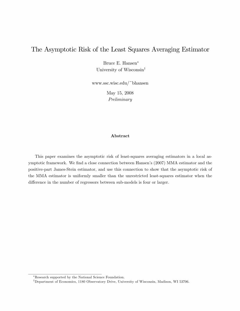
The Asymptotic Risk of the Least Squares Averaging Estimator

Bruce E. Hansen�

University of Wisconsiny

www.ssc.wisc.edu/~bhansen

May 15, 2008Preliminary

Abstract

This paper examines the asymptotic risk of least-squares averaging estimators in a local as-

ymptotic framework. We �nd a close connection between Hansen�s (2007) MMA estimator and the

positive-part James-Stein estimator, and use this connection to show that the asymptotic risk of

the MMA estimator is uniformly smaller than the unrestricted least-squares estimator when the

di¤erence in the number of regressors between sub-models is four or larger.

�Research supported by the National Science Foundation.yDepartment of Economics, 1180 Observatory Drive, University of Wisconsin, Madison, WI 53706.

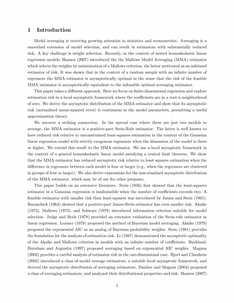
1 Introduction

Model averaging is receiving growing attention in statistics and econometrics. Averaging is a

smoothed extension of model selection, and can result in estimators with substantially reduced

risk. A key challenge is weight selection. Recently, in the context of nested homoskedastic linear

regression models, Hansen (2007) introduced the the Mallows Model Averaging (MMA) estimator

which selects the weights by minimization of a Mallows criterion, the latter motivated as an unbiased

estimator of risk. It was shown that in the context of a random sample with an in�nite number of

regressors the MMA estimator is asymptotically optimal in the sense that the risk of the feasible

MMA estimator is asymptotically equivalent to the infeasible optimal averaging estimator.

This paper takes a di¤erent approach. Here we focus on �nite-dimensional regression and explore

estimation risk in a local asymptotic framework where the coe¢ cients are in a root-n neighborhood

of zero. We derive the asymptotic distribution of the MMA estimator and show that its asymptotic

risk (normalized mean-squared error) is continuous in the model parameters, permitting a useful

approximation theory.

We uncover a striking connection. In the special case where there are just two models to

average, the MMA estimator is a positive-part Stein-Rule estimator. The latter is well known to

have reduced risk relative to unconstrained least-squares estimation in the context of the Gaussian

linear regression model with strictly exogenous regressors when the dimension of the model is three

or higher. We extend this result to the MMA estimator. We use a local asymptotic framework in

the context of a general homoskedastic linear model satisfying a central limit theorem. We show

that the MMA estimator has reduced asymptotic risk relative to least squares estimation when the

di¤erence in regressors between each model is four or larger (e.g., when the regressors are clustered

in groups of four or larger). We also derive expressions for the non-standard asymptotic distribution

of the MMA estimator, which may be of use for other purposes.

This paper builds on an extensive literature. Stein (1956) �rst showed that the least-squares

estimator in a Gaussian regression is inadmissible when the number of coe¢ cients exceeds two. A

feasible estimator with smaller risk than least-squares was introduced by James and Stein (1961).

Baranchick (1964) showed that a positive-part James-Stein estimator has even smaller risk. Akaike

(1973), Mallows (1973), and Schwarz (1978) introduced information criterion suitable for model

selection. Judge and Bock (1978) provided an extensive evaluation of the Stein-rule estimator in

linear regression. Leamer (1978) proposed the method of Bayesian model averaging. Akaike (1979)

proposed the exponential AIC as an analog of Bayesian probability weights. Stein (1981) provides

the foundation for the analysis of estimation risk. Li (1987) demonstrated the asymptotic optimality

of the Akaike and Mallows criterion in models with an in�nite number of coe¢ cients. Buckland,

Burnham and Augustin (1997) proposed averaging based on exponential AIC weights. Magnus

(2002) provides a careful analysis of estimator risk in the one-dimensional case. Hjort and Claeskens

(2003) introduced a class of model average estimators, a suitable local asymptotic framework, and

derived the asymptotic distribution of averaging estimators. Danilov and Magnus (2004) proposed

a class of averaging estimators, and analyzed their distributional properties and risk. Hansen (2007)

1

proposed the MMA estimator and demonstrated its asymptotic optimality in the sense of Li (1987).

Hansen and Racine (2007) proposed a jackknife model averaging (JMA) estimator appropriate for

regression models with heteroskedasticity and demonstrated its asymptotic optimality.

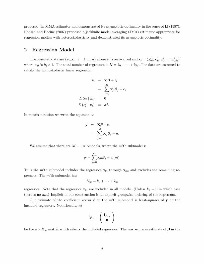
2 Regression Model

The observed data are fyi;xi : i = 1; :::; ng where yi is real-valued and xi = (x00i;x01i;x02i; :::;x0Mi)0

where xji is kj � 1. The total number of regressors is K = k0+ � � �+ kM : The data are assumed tosatisfy the homoskedastic linear regression

yi = x0i� + ei

=

MXj=0

x0ji�j + ei

E (ei j xi) = 0

E�e2i j xi

�= �2:

In matrix notation we write the equation as

y = X� + e

=

MXj=0

Xj�j + e:

We assume that there are M + 1 submodels, where the m�th submodel is

yi =

mXj=0

xji�j + ei(m):

Thus the m�th submodel includes the regressors x0i through xmi and excludes the remaining re-

gressors. The m�th submodel has

Km = k0 + � � �+ km

regressors. Note that the regressors x0i are included in all models. (Unless k0 = 0 in which case

there is no x0i.) Implicit in our construction is an explicit groupwise ordering of the regressors.

Our estimate of the coe¢ cient vector � in the m�th submodel is least-squares of y on the

included regressors. Notationally, let

Sm =

IKm

0

!

be the n�Km matrix which selects the included regressors. The least-squares estimate of � in the

2

m�th submodel is

�m = Sm�S0mX

0XSm��1

S0mX0y

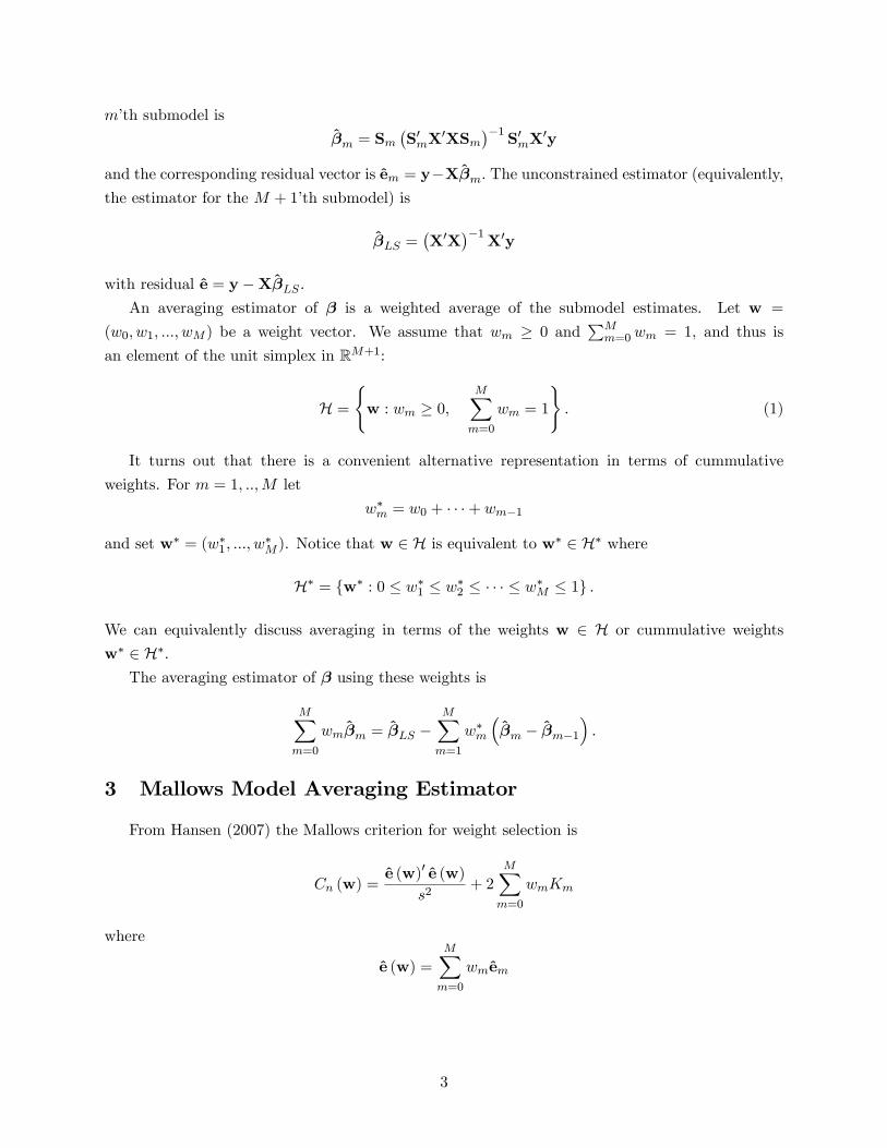
and the corresponding residual vector is em = y�X�m: The unconstrained estimator (equivalently,the estimator for the M + 1�th submodel) is

�LS =�X0X

��1X0y

with residual e = y �X�LS .An averaging estimator of � is a weighted average of the submodel estimates. Let w =

(w0; w1; :::; wM ) be a weight vector. We assume that wm � 0 andPMm=0wm = 1, and thus is

an element of the unit simplex in RM+1:

H =

(w : wm � 0;

MXm=0

wm = 1

): (1)

It turns out that there is a convenient alternative representation in terms of cummulative

weights. For m = 1; ::;M let

w�m = w0 + � � �+ wm�1

and set w� = (w�1; :::; w�M ). Notice that w 2 H is equivalent to w� 2 H� where

H� = fw� : 0 � w�1 � w�2 � � � � � w�M � 1g :

We can equivalently discuss averaging in terms of the weights w 2 H or cummulative weights

w� 2 H�:The averaging estimator of � using these weights is

MXm=0

wm�m = �LS �MXm=1

w�m

��m � �m�1

�:

3 Mallows Model Averaging Estimator

From Hansen (2007) the Mallows criterion for weight selection is

Cn (w) =e (w)0 e (w)

s2+ 2

MXm=0

wmKm

where

e (w) =MXm=0

wmem

3

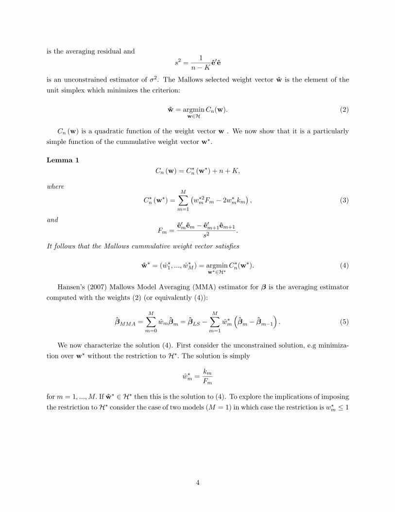
is the averaging residual and

s2 =1

n�K e0e

is an unconstrained estimator of �2. The Mallows selected weight vector w is the element of the

unit simplex which minimizes the criterion:

w = argminw2H

Cn(w): (2)

Cn (w) is a quadratic function of the weight vector w . We now show that it is a particularly

simple function of the cummulative weight vector w�:

Lemma 1Cn (w) = C

�n (w

�) + n+K;

where

C�n (w�) =

MXm=1

�w�2mFm � 2w�mkm

�; (3)

and

Fm =e0mem � e0m+1em+1

s2:

It follows that the Mallows cummulative weight vector satis�es

w� = (w�1; :::; w�M ) = argmin

w�2H�C�n(w

�): (4)

Hansen�s (2007) Mallows Model Averaging (MMA) estimator for � is the averaging estimator

computed with the weights (2) (or equivalently (4)):

�MMA =

MXm=0

wm�m = �LS �MXm=1

w�m

��m � �m�1

�: (5)

We now characterize the solution (4). First consider the unconstrained solution, e.g minimiza-

tion over w� without the restriction to H�: The solution is simply

w�m =kmFm

form = 1; :::;M: If w� 2 H� then this is the solution to (4). To explore the implications of imposingthe restriction toH� consider the case of two models (M = 1) in which case the restriction is w�m � 1

4

and the constrained solution takes the simple form

w�1 =

8>>>><>>>>:k1F1

ifk1F1< 1

1 ifk1F1� 1

which implies that the weights take the form

w0 =

8>>>><>>>>:k1F1

ifk1F1< 1

1 ifk1F1� 1

w1 =

8>>>><>>>>:1� k1

F1ifk1F1< 1

0 ifk1F1� 1

The unrestricted estimate of the weight for model 0 is k1=F1: When this is infeasible (exceeds 1)

then the weight is truncated at the boundary and the weight for model 1 is set to zero �model

1 is eliminated from the estimator. This is a general feature of the solutions to (4) �when the

uncontrained solution is infeasible, the constraints are imposed by elimination of submodels.

Thus when M = 1 the MMA estimator is simply

�MMA = �LS ���LS � �0

�� k1F11

�k1F1� 1�+ 1

�k1F1> 1

��:

This is a member of the �positive part James-Stein�class of estimators. This is easiest to see when

k0 = 0 so that there is no �0: In this case F1 = �0LSX

0X�LS=s2 and

�MMA = �LS

1� s2k1

�0LSX

0X�LS

!+

(6)

where (a)+ is the positive part operator. This is a positive-part James-Stein estimator with penalty

k1: In the Gaussian linear regression model with strictly exogeneous regressors this estimator is

known to have reduced risk relative to �LS when k1 � 4: If k1 in the de�nition (6) is replaced withk1 � 2 (the classic choice) then there is reduction in risk relative to �LS when k1 � 3:

For M > 1 is it cumbersome to explicitly write down the solutions. Instead, we have the

following characterization.

Lemma 2 The solution to (4) takes the following form. There is a (random) integer J � M and

5

index set fm0;m1; :::;mJg � f0; 1; :::;Mg; such that if we de�ne

�kj = kmj�1+1 + � � �+ kmj ; (7)

�Fj = Fmj�1+1 + � � �+ Fmj ; (8)

and

�w�j =�kj�Fj1

� �kj�Fj� 1�+ 1

� �kj�Fj> 1

�; (9)

then for m = mj�1 + 1; :::;mj ; the cummulative weights equal

w�m = �w�j : (10)

The cummulative weights (10) are continuous functions of (F1; :::; FM ): An algorithm which �nds

the index set fm0;m1; :::;mJg is as follows:

1. Start with the set of models fm0;m1; :::;mJg = f0; 1; :::;Mg:

2. Calculate �kj and �Fj using (7)-(8).

3. For 0 < j < M; eliminate any mj in the set fm0;m1; :::;mJg for which

�kj�Fj��kj+1�Fj+1

:

4. Repeat steps 2 and 3 until�k1�F1<�k2�F2< � � � <

�kJ�FJ:

5. Set �w�j by (9) and w�m by (10). This is the solution to (4).

Given the representation in Lemma 2, we see that the MMA estimator can be also written in

terms of the weights (9):

�MMA = �LS �JXj=1

�w�j

��mj

� �mj�1

�:

This representation is conditional on the index set fm0;m1; :::;mJg which is a function of the data.

4 Asymptotic Distribution

The distribution of the estimators discussed in the previous section are invariant to �0; the

coe¢ cients on the included regressors, but are not invariant to the other coe¢ cients. To develop

an asymptotic theory which is continuous in their values we follow Hjort and Claesken (2004) and

use a canonical local asymptotic framework when �j is in a local n�1=2 neighborhood of zero.

6

We start by describing the asymptotic distribution of the LS estimator in the m�th model.

The following high level conditions embrace cross-section, panel, and time-series applications, but

impose homoskedasticity.

Assumption 1 As n ! 1; n�1X0X !p Q, n�1=2X0e !d N�0; �2Q

�; and for j � 1; n1=2�j !

�j :

The MMA estimator depends on the submodel estimators �m and statistics Fm:We now present

their asymptotic (joint) distribution. Let V = �2Q�1 be the asymptotic variance of the uncon-

strained estimator �LS , let �0 = 0; and set � = (�00; �

01; :::; �

0M )

0:

Theorem 1 As n!1;pn��LS � �

�d�! Z� � (11)

pn��m � �m�1

�d�! AmZ (12)

and

Fmd�! Z0WmZ; (13)

jointly in m = 0; :::;M; where Z � N(�;V) ;

Am = Sm�S0mV

�1Sm��1

S0mV�1 � Sm�1

�S0m�1V

�1Sm�1��1

S0m�1V�1; (14)

and

Wm = V�1Am: (15)

From Lemma 1 and Theorem 1 we can deduce the asymptotic distribution of the MMA criterion,

weights, and estimator.

Theorem 2 As n!1;

C�n (w�)

d�! C� (w� j Z) =MXm=1

�w�2mZ

0WmZ� 2w�mkm�; (16)

w�d�! w� (Z) = argmin

w�2H�C� (w� j Z) ; (17)

andpn��MMA � �

�d�! Z�

MXm=1

w�m (Z)AmZ� � = Z�JXj=1

�w�j (Z) �AjZ� � (18)

where�Aj = Amj�1+1 + � � �+Amj : (19)

The solution to (17) takes the following form. There is an integer J (Z) � M and index set

7

fm0 (Z) ;m1 (Z) ; :::;mJ (Z)g � f0; 1; :::;Mg; functions of Z; such that if we de�ne

�Wj =Wmj�1+1 + � � �+Wmj (20)

and

�w�m (Z) =�kj

Z0 �WjZ1

� �kj

Z0 �WjZ� 1�+ 1

� �kj

Z0 �WjZ> 1

�(21)

then for m = mj�1 + 1; :::;mj ;

w�m (Z) = �w�j (Z) : (22)

The weights (22) are continuous functions of Z: The index set fm0 (Z) ;m1 (Z) ; :::;mJ (Z)g is de-termined by the algorithm described in Lemma 2, with (21), (22) and Z0 �WjZ; replacing (9), (10)

and �Fj ; respectively.

These distributions are functions of the normal random vector Z: We use these results in the

next section to compute the asymptotic risk of the MMA estimator. However, these distributional

results may be useful for alternative purposes, including inference.

5 Asymptotic Risk

The risk of �MMA for � under quadratic weighted loss is

trE

���MMA � �

���MMA � �

�0W

�= E

���MMA � �

�0W��MMA � �

��where W is a weight matrix. Setting W = nV�1 is convenient to minimized the dependence on

nuisance parameters. Further simpli�cation can be obtained by taking the limit as n tends to

in�nity. This yields the risk

limn!1

E

�n��MMA � �

�0V�1

��MMA � �

��: (23)

Unfortunately the expectation may not exist for �nite n without imposing strong conditions.

When the expectation exists (and is uniformly integrable) the limit in (23) equals the expectation

of the asymptotic distribution of the random variable in (23). A simple solution is to de�ne the

asymptotic risk directly as this asymptotic expectation. That is, since (18) shows that

pn��MMA � �

�d�! Z�

MXm=1

�w�m (Z)AmZ� �

8

then we de�ne the asymptotic risk of �MMA as

RMMA = E

0@ Z� MXm=1

�w�m (Z)AmZ� �!0V�1

Z�

MXm=1

�w�m (Z)AmZ� �!1A :

Similarly, since (11) shows thatpn��LS � �

�d�! Z � �; then we de�ne the asymptotic risk of

�LS as

RLS = E�(Z� �)0V�1 (Z� �)

�= K:

We are now in a position to calculate the asymptotic risk of the MMA estimator.

Theorem 3RMMA = K � E (q (Z)) (24)

where

q (Z) =JXj=1

�kj��kj � 4

�Z0 �WjZ

1��kj � Z0 �WjZ

�+

JXj=1

�2�kj � Z0 �WjZ

�1��kj > Z

0 �WjZ�: (25)

If km � 4 for m � 1 then q (Z) � 0 and

RMMA � RLS : (26)

If M = 1 or km � 5 then the inequality in (26) is strict.The risk of �MMA depends on unknowns only through Z

0 �WmZ; which are non-central chi-square

with degrees of freedom km and non-centrality parameters

��2m = �

0 �Wm�: (27)

Equations (24)-(25) give an expression for the asymptotic risk of the MMA estimator. Our most

important result is equation (26) which states that the asymptotic risk of the MMA estimator is less

than that of the least-squares estimator, uniformly in the parameter space, so long as the dimension

of each regression group km is four or larger. This occurs when the regressors are clustered into

groups of at least four. [Note: I expect the weak inequality in (26) can be made into a strict

inequality.] This result reinforces the view that the MMA estimator is similar to a generalized

James-Stein estimator. One interesting implication of Theorem 3 is that (26) holds for all values of

�; so it does not require that the regressors have been �correctly�ordered. For example, suppose

that �1 = 0 and �2 6= 0 so that the �correct�model should include x0i and x2i but exclude x1i; sothat the ordering is incorrect. Even in this case, the MMA estimator achieves reduced risk relative

to unrestricted least-squares. This result is surprising.

The �nal statement of the theorem is that the asymptotic risk depends only on the dimension

km of the variables xmi and the non-centrality parameters ��m: The risk is invariant to other features

of the parameters and data distributions.

9

6 Quantitative Illustration

In this section we display quantitative representations of the risk of the averaging estimators.

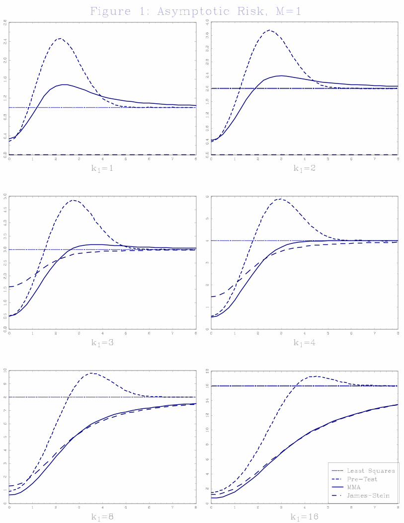
We �rst consider the two-model case M = 1: Theorem 3 shows that the asymptotic risk of the

MMA estimator is completely determined by k1 and ��1: In Figure 1 we display the asymptotic

risk as a function of ��1; for k1 = 1; 2, 3, 4, 8, and 16. We display the asymptotic risk of four

estimators: MMA, least-squares, James-Stein, and the traditional asymptotic pre-test estimator

with a 5% critical value. Least-squares is our baseline estimator, with an asymptotic risk of k1:

As is well known, the pre-test estimator has quite poor risk properties: The risk of the MMA

estimator is mixed for k1 = 1 and k1 = 2; but is excellent for k1 � 3: The MMA estimator has

smaller risk than the James-Stein estimator for small ��1 but the reverse for large ��1:

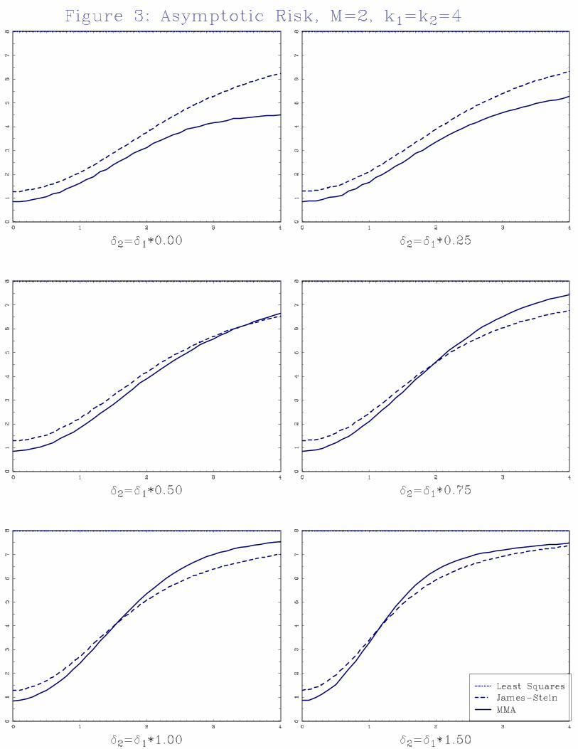
The three-model caseM = 2 is slightly more complicated. Theorem 3 shows that the asymptotic

risk depends on k1; k2; ��1 and ��2: To keep things simple we focus on k1 = k2 and consider only

k1 = k2 = 3 (e.g. K = 6) and k1 = k2 = 4 (K = 8): We plot the asymptotic risk of the least

squares, James-Stein, and MMA estimators as a function of ��1; varying ��2 = c��1 with c = 0; .25,

.50, .75, 1.00 and 1.50. These choices are motivated by the assumption that MMA is designed for

the nested regression model, so that ��1 � ��2 (or 0 � c < 1) is the leading case of interest, and

c � 1 is included as a robustness check. Figure 2 displays the asymptotic risk for k1 = k2 = 3; andFigure 3 displays the asymptotic risk for k1 = k2 = 4:

Even in Figure 2 all averaging estimators have nearly uniformly smaller risk than least squares

(it is guarenteed in Figure 3 by Theorem 3). In most �gures the risk of least squares (6 in Figure 2,

8 in Figure 3) is at the top of the display. Notice that for small ��1 the risk of MMA is substantially

smaller than least-squares.

For small �2 the risk of the MMA estimator is uniformly smaller than the other estimators.

This is re�ecting the nested ordering inherit in MMA. For larger ��2 neither MMA nor James-Stein

uniformly dominate the other.

10

7 Appendix

Proof of Lemma 1: Let Lm = e0mem denote the sum-of-squared errors in the m�th model.

Note that Lj � Lj+1 and e0j ek = Lj for k < j by the properties of the LS residuals. The Mallowscriterion is

Cn (w) = s�2

MXj=0

MXm=0

wjwmLj_m + 2MXm=0

wmKm: (28)

The �rst term in (28) can be rewritten as

s�2�w20L0 +

�w21 + 2w1w0

�L1 +

�w22 + 2w2 (w0 + w1)

�L2 + � � �+

�w2M + 2wM (w0 + � � �+ wM�1)

�LM�

= s�2�w20L0 +

�(w0 + w1)

2 � w20�L1 +

�(w0 + w1 + w2)

2 � (w0 + w1)2�L2

+ � � �+�(w0 + � � �+ wM )2 � (w0 + � � �+ wM�1)

2��LM

= s�2�w20 (L0 � L1) + (w0 + w1)

2 (L1 � L2)

+ � � �+ (w0 + � � �+ wM�1)2 (LM�1 � LM ) + (w0 + � � �+ wM )2

�LM

=

MXm=1

w�2mFm + n�K: (29)

the �nal line using the fact that s�2LM = n�K:The second term in (28) is twice

MXm=0

wmKm = w0 (K0 �K1) + (w0 + w1) (K1 �K2) + � � �

+(w0 + � � �+ wM�1) (KM�1 �KM ) + (w0 + � � �+ wM )KM

= �MXm=1

w�mkm +K: (30)

Summing (29) and twice (30), we �nd C�n (w�) as de�ned in (3). �

Proof of Lemma 2: [incomplete] The solution to (4) with either be interior to H�, in whichcase w�m = km=Fm for all m; or on the boundary of H�: As H� is a convex polyhedron, its boundaryconsists of sets of binding contraints, each constraint corresponding to excluding a speci�c model

(that is, setting w�m = w�m+1 and thus wm = 0): Finding the solution is thus equivalent to �nding

the set of included and excluded models.

Suppose that the the set of included models is fm1; :::;mJg:We want to show that the solutiontakes the form (10). The restriction of included models to the set fm1; :::;mJg means that forj = 1; :::; J and ` = mj�1 + 1; :::;mj ;

w�` = w�mj

(31)

11

and for ` � mJ + 1;

w�` = 1 (32)

Thus (4) can be written as

argminw�m1 ;:::;w

�mJ

JXj=1

mjX`=mj�1+1

�w�2` F` � 2w�`k`

�

= argminw�m1 ;:::;w

�mJ

JXj=1

(mj �mj�1)

0@w�2mj

0@ mjX`=mj�1+1

F`

1A� 2w�mj

0@ mjX`=mj�1+1

k`

1A1A= argmin

w�m1 ;:::;w�mJ

JXj=1

(mj �mj�1)�w�2mj

�Fj � 2w�mj�kj

�which has the solution

w�mj=�kj�Fj:

Combined with (31) and (32) this implies (10) as desired.

We now want to establish that the algorithm described in the Lemma implements the solution

to (4). As mentioned above, it is su¢ cient to describe how to �nd the set of included models is

fm1; :::;mJg. Since the analysis of the problem given any set of models is identical, it is su¢ cient

to describe how to eliminate models from the set of included models. By sequential elimination,

the included set will be found. We now describe how to do so.

The Lagrange multiplier problem for (4) can be written as

minwm2R; �m�0

MXm=1

�1

2w�2mFm � w�mkm

��

MXm=1

�m�w�m+1 � w�m

�where we �x wM+1 = 1: The �m are non-negative Lagrange multipliers imposing the inequality

constraints w�m+1 � w�m � 0: The �rst-order conditions for the cummulative weights can be solvedto �nd

w�m =km + �m�1 � �m

Fm(33)

The events f�m > 0g ;�w�m = w

�m+1

and fwm = 0g are equivalent.

We claim that km=Fm > km+1=Fm+1 implies that w�m = w�m+1; which we prove by contradiction.

That is, suppose that km=Fm > km+1=Fm+1 yet w�m < w�m+1: Then �m = 0 (as the constraint is

not binding). Using (33) for w�m and w�m+1 and setting �m = 0; it follows that

w�m =km + �m�1

Fm< w�m+1 =

km+1 � �m+1Fm+1

orkmFm

� km+1Fm+1

< ���m�1Fm

+�m+1Fm+1

�� 0 (34)

12

the �nal inequality since �j � 0 and Ff � 0 for all j: But (34) contradicts the assumption that

km=Fm > km+1=Fm+1: The contradiction establishes the claim that km=Fm > km+1=Fm+1 implies

that w�m = w�m+1:

We have established that starting with the set of models f1; :::;Mg, if km=Fm > km+1=Fm+1

then model m can be eliminated, which establishes the elimination set in the algorithm. �

Lemma 3 For Am and Wm de�ned in (14) and (15), A0mV�1Am = Wm and for m 6= `;

A0mV�1A` = 0:

Proof: Since the models are nested, if m � ` then Sm is in the range space of S` and thereforeSm = S`T for some matrix T. It follows that

S`�S0`V

�1S`��1

S0`V�1Sm = S`

�S0`V

�1S`��1

S0`V�1S`T = S`T = Sm:

Thus S`�S0`V

�1S`��1

S0`V�1 is a projection operator. This allows us to calculate that

A0mV�1Am = V�1Sm

�S0mV

�1Sm��1

S0mV�1Sm

�S0mV

�1Sm��1

S0mV�1

�V�1Sm�S0mV

�1Sm��1

S0mV�1Sm�1

�S0m�1V

�1Sm�1��1

S0m�1V�1

�V�1Sm�1�S0m�1V

�1Sm�1��1

S0m�1V�1Sm

�S0mV

�1Sm��1

S0mV�1

+V�1Sm�1�S0m�1V

�1Sm�1��1

S0m�1V�1Sm�1

�S0m�1V

�1Sm�1��1

S0m�1V�1

= V�1Sm�S0mV

�1Sm��1

S0mV�1

�V�1Sm�1�S0m�1V

�1Sm�1��1

S0m�1V�1

�V�1Sm�1�S0m�1V

�1Sm�1��1

S0m�1V�1

+V�1Sm�1�S0m�1V

�1Sm�1��1

S0m�1V�1

= Wm:

Suppose m � `� 1: Then

A0mV�1A` = V�1Sm

�S0mV

�1Sm��1

S0mV�1S`

�S0`V

�1S`��1

S0`V�1

�V�1Sm�S0mV

�1Sm��1

S0mV�1S`�1

�S0`�1V

�1S`�1��1

S0`�1V�1

�V�1Sm�1�S0m�1V

�1Sm�1��1

S0m�1V�1S`

�S0`V

�1S`��1

S0`V�1

+V�1Sm�1�S0m�1V

�1Sm�1��1

S0m�1V�1S`�1

�S0`�1V

�1S`�1��1

S0`�1V�1

= V�1Sm�S0mV

�1Sm��1

S0mV�1

�V�1Sm�S0mV

�1Sm��1

S0mV�1

= 0

Similarly if ` � m� 1 then A0mV�1A` = 0; completing the proof.

13

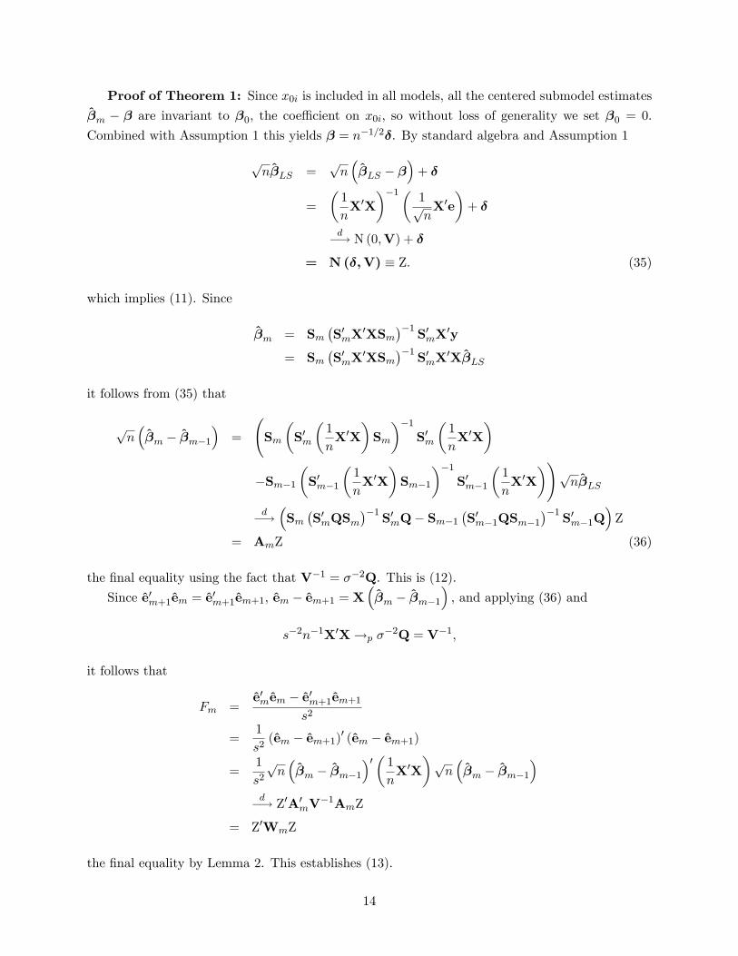
Proof of Theorem 1: Since x0i is included in all models, all the centered submodel estimates�m � � are invariant to �0; the coe¢ cient on x0i; so without loss of generality we set �0 = 0.

Combined with Assumption 1 this yields � = n�1=2�. By standard algebra and Assumption 1

pn�LS =

pn��LS � �

�+ �

=

�1

nX0X

��1� 1pnX0e

�+ �

d�! N(0;V) + �

= N(�;V) � Z: (35)

which implies (11). Since

�m = Sm�S0mX

0XSm��1

S0mX0y

= Sm�S0mX

0XSm��1

S0mX0X�LS

it follows from (35) that

pn��m � �m�1

�=

Sm

�S0m

�1

nX0X

�Sm

��1S0m

�1

nX0X

�

�Sm�1�S0m�1

�1

nX0X

�Sm�1

��1S0m�1

�1

nX0X

�!pn�LS

d�!�Sm�S0mQSm

��1S0mQ� Sm�1

�S0m�1QSm�1

��1S0m�1Q

�Z

= AmZ (36)

the �nal equality using the fact that V�1 = ��2Q. This is (12).

Since e0m+1em = e0m+1em+1; em � em+1 = X

��m � �m�1

�; and applying (36) and

s�2n�1X0X!p ��2Q = V�1;

it follows that

Fm =e0mem � e0m+1em+1

s2

=1

s2(em � em+1)0 (em � em+1)

=1

s2pn��m � �m�1

�0� 1nX0X

�pn��m � �m�1

�d�! Z0A0mV

�1AmZ

= Z0WmZ

the �nal equality by Lemma 2. This establishes (13).

14

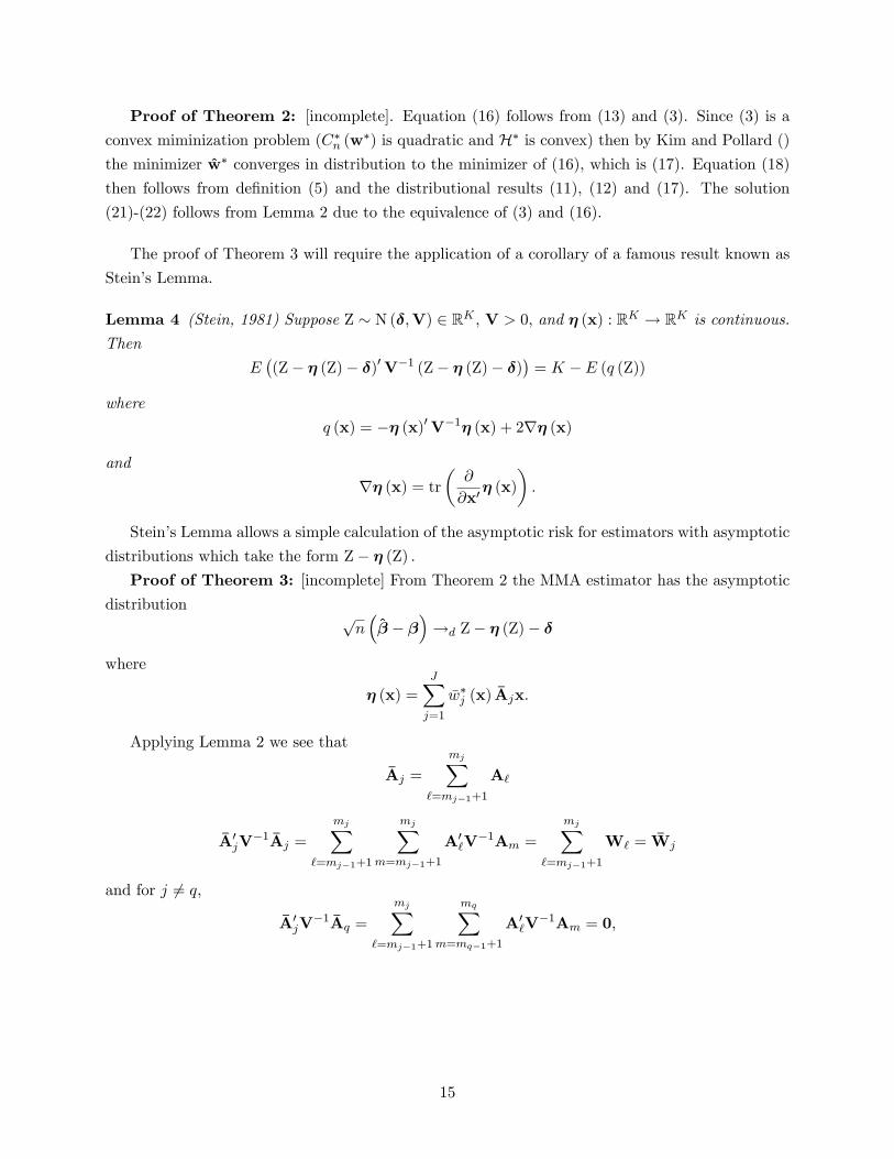
Proof of Theorem 2: [incomplete]. Equation (16) follows from (13) and (3). Since (3) is a

convex miminization problem (C�n (w�) is quadratic and H� is convex) then by Kim and Pollard ()

the minimizer w� converges in distribution to the minimizer of (16), which is (17). Equation (18)

then follows from de�nition (5) and the distributional results (11), (12) and (17). The solution

(21)-(22) follows from Lemma 2 due to the equivalence of (3) and (16).

The proof of Theorem 3 will require the application of a corollary of a famous result known as

Stein�s Lemma.

Lemma 4 (Stein, 1981) Suppose Z � N(�;V) 2 RK ; V > 0; and � (x) : RK ! RK is continuous.

Then

E�(Z� � (Z)� �)0V�1 (Z� � (Z)� �)

�= K � E (q (Z))

where

q (x) = �� (x)0V�1� (x) + 2r� (x)

and

r� (x) = tr�@

@x0� (x)

�:

Stein�s Lemma allows a simple calculation of the asymptotic risk for estimators with asymptotic

distributions which take the form Z� � (Z) :Proof of Theorem 3: [incomplete] From Theorem 2 the MMA estimator has the asymptotic

distributionpn�� � �

�!d Z� � (Z)� �

where

� (x) =

JXj=1

�w�j (x) �Ajx:

Applying Lemma 2 we see that

�Aj =

mjX`=mj�1+1

A`

�A0jV�1 �Aj =

mjX`=mj�1+1

mjXm=mj�1+1

A0`V�1Am =

mjX`=mj�1+1

W` = �Wj

and for j 6= q;

�A0jV�1 �Aq =

mjX`=mj�1+1

mqXm=mq�1+1

A0`V�1Am = 0;

15

and hence

� (x)0V�1� (x) =

JXj=1

��w�j (x)

�2x0 �A0jV

�1 �Ajx

=JXj=1

��w�j (x)

�2x0 �Wjx:

Recalling that

�w�j (x) =�kj

x0 �Wjx1

� �kj

x0 �Wjx� 1�+ 1

� �kj

x0 �Wjx> 1

�we �nd

� (x)0V�1� (x) =JXj=1

�k2j

x0 �Wjx1

� �kj

x0 �Wjx� 1�+

JXj=1

�x0 �Wjx

�1

� �kj

x0 �Wjx> 1

�:

Next, since

� (x) =JXj=1

�w�j (x) �Ajx

=

JXj=1

�Ajx�kj�

x0 �Wjx�1� �kj

x0 �Wjx� 1�+

JXj=1

�Ajx1

� �kj

x0 �Wjx> 1

�

then

tr

�@

@x0� (x)

�= tr

0@ JXj=1

�Aj

"�kj�

x0 �Wjx� � 2�kj�

x0 �Wjx�2xx0 �Wj

#1

� �kj

x0 �Wjx� 1�+

JXj=1

�Aj1

� �kj

x0 �Wjx> 1

�1A=

JXj=1

�k2j � 2�kj�x0 �Wjx

�! 1� �kj

x0 �Wjx� 1�+

JXj=1

�kj1

� �kj

x0 �Wjx> 1

�

(since tr��Aj�= �kj) and

r� (x) =JXj=1

�k2j � 2�kjx0 �Wjx

!1

� �kj

x0 �Wjx� 1�+

JXj=1

�kj1

� �kj

x0 �Wjx> 1

�:

Hence

q (x) = �� (x)0V�1� (x) + 2r� (x)

=JXj=1

�kj��kj � 4

�x0 �Wjx

!1

� �kj

x0 �Wjx� 1�+

JXj=1

�2�kj �

�x0 �Wjx

��1

� �kj

x0 �Wjx> 1

�:

16

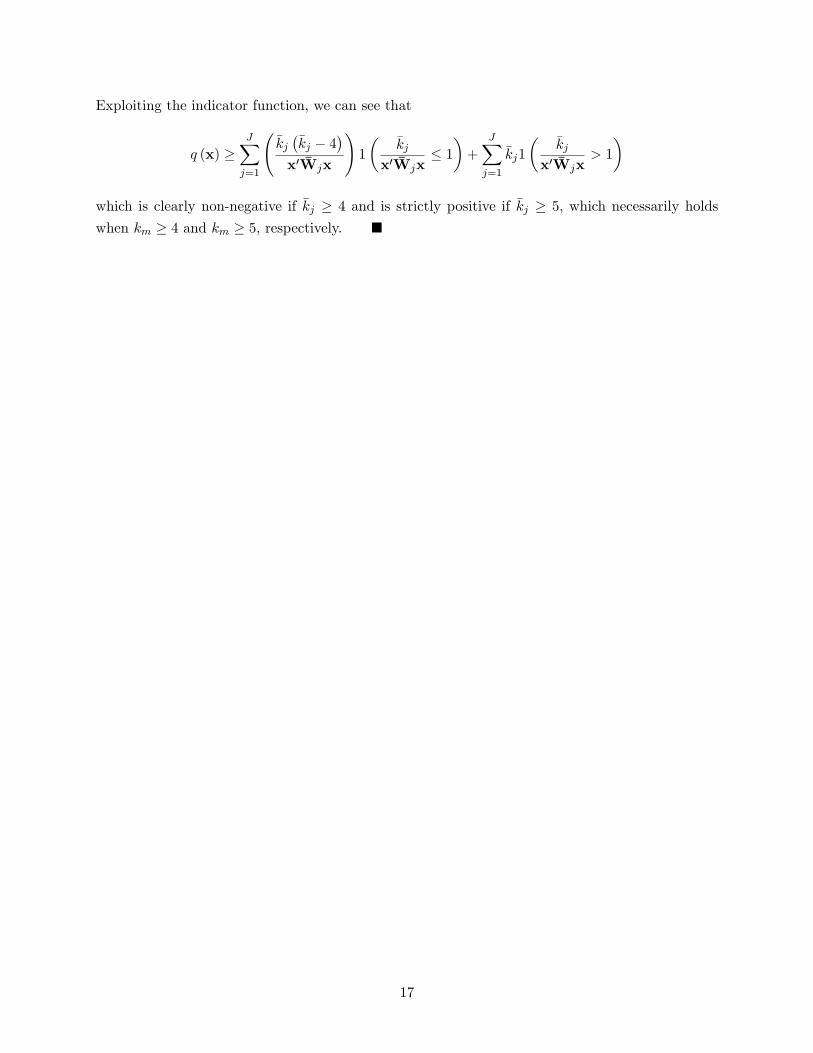
Exploiting the indicator function, we can see that

q (x) �JXj=1

�kj��kj � 4

�x0 �Wjx

!1

� �kj

x0 �Wjx� 1�+

JXj=1

�kj1

� �kj

x0 �Wjx> 1

�

which is clearly non-negative if �kj � 4 and is strictly positive if �kj � 5; which necessarily holds

when km � 4 and km � 5; respectively. �

17

References

[1] Akaike, Hirotsugu (1973): �Information theory and an extension of the maximum likelihood

principle.�In B. Petroc and F. Csake, eds., Second International Symp. on Information Theory.

[2] Akaike, Hirotsugu, (1979): �A Bayesian extension of the minimum AIC procedure of autore-

gressive model �tting,�Biometrika, 66, 237-242.

[3] Baranchick, A. (1964): �Multiple regression and estimation of the mean of a multivariate

normal distribution,�Technical Report No. 51, Department of Statistics, Stanford University.

[4] Buckland, S.T., K.P. Burnhamn and N.H. Augustin (1997): �Model Selection: An Integral

Part of Inference,�Biometrics, 53, 603-618.

[5] Danilov, Dmitry and Jan R. Magnus (2004): �On the harm that ignoring pretesting can cause,�

Journal of Econometrics, 122, 27-64.

[6] Hansen, Bruce E., (2007): �Least Squares Model Averaging,�Econometrica, 75, 1175-1189.

[7] Hansen, Bruce E. and Je¤rey S. Racine (2007): �Jackknife Model Averaging,�working paper.

[8] Hjort, Nils Lid and Gerda Claeskens (2003): �Frequentist Model Average Estimators,�Journal

of the American Statistical Association, 98, 879-899.

[9] James W. and Charles M. Stein (1961): �Estimation with quadratic loss,�Proc. Fourth Berke-

ley Symp. Math. Statist. Probab., 1, 361-380.

[10] Judge, George and M. E. Bock (1978): The Statistical Implications of Pre-test and Stein-rule

Estimators in Econometrics, North-Holland.

[11] Leamer, Edward E. (1978): Speci�cation Searches: Ad Hoc Inference with Nonexperimental

Data, Wiley, New York.

[12] Li, Ker-Chau (1987): �Asymptotic optimality for Cp; CL; cross-validation and generalized

cross-validation: Discrete Index Set,� Annals of Statistics, 15, 958-975.

[13] Magnus, Jan R. (2002): �Estimation of the mean of a univariate normal distribution with

known variance,�Econometrics Journal, 5, 225-236.

[14] Mallows, Colin L. (1973): �Some comments on Cp;�Technometrics, 15, 661-675.

[15] Schwarz, G. (1978): �Estimating the dimension of a model,�Annals of Statistics, 6, 461-464.

[16] Stein, Charles M. (1956): �Inadmissibility of the usual estimator for the mean of a multivariate

normal distribution,�Proc. Third Berkeley Symp. Math. Statist. Probab., 1, 197-206.

[17] Stein, Charles M. (1981): �Estimation of the mean of a multivariate normal distribution,�

Annals of Statistics, 9, 1135-1151.

18