The Geography of Sustainability: Agglomeration, Global Economy and Environment

The geography of sustainability: agglomeration, global economy and environment Fifth Urban Research Symposium 2009

THE GEOGRAPHY OF SUSTAINABILITY:

AGGLOMERATION, GLOBAL ECONOMY AND ENVIRONMENT

Fabio GRAZI a, Henri WAISMAN a and Jeroen C.J.M. van den BERGH b,c

([email protected]; [email protected]; [email protected])

a International Research Centre on the Environment and Development (CIRED)

b ICREA, Department of Economics and Economic History & Institute of Environmental Science and Technology, Autonomous University of Barcelona.

c Faculty of Economics and Business Administration & Institute for Environmental Studies, Vrije Universiteit

ABSTRACT

This paper develops a theoretical model to formalize the notions of spatial sustainability and sustainable trade. It incorporates agglomeration effects, production- and trade-related environmental externalities, and dynamics of migration and pollution. The model can generate different spatial configurations of the economy and transitions between these. Among sustainable economies, a spatially asymmetric configuration generally performs the best in terms of global welfare. The results reflect welfare-offsetting trade and spatial structure effects in environmental regulation. Our model is conceptually innovative in formalizing continuously variable degrees and multi-regional heterogeneity of economic concentration in space, and in distinguishing between environmental externalities and environmental sustainability. (JEL F12, F18, Q56, R12).

Keywords: Pollution externality, Regional and Urban economics, Trade, Welfare.

1

mailto:[email protected];%[email protected]

mailto:[email protected]


THE GEOGRAPHY OF SUSTAINABILITY:

AGGLOMERATION, GLOBAL ECONOMY AND ENVIRONMENT

I. INTRODUCTION Translating the notion of sustainable development into concrete principles and actions at local, regional, and national levels, where governance is most concrete and effective, has turned out to be difficult (OECD, 2007). One reason is that there is not an agreed upon framework for studying the spatial dimension of sustainable development. This would require a combination of dynamic, spatial, and economic building blocks. A natural way to operationalize such a framework is to adopt a system of regions and trade relations.

This paper presents a theoretical framework to analyze the impact of spatial configurations of economic activities on the (un)sustainability of the economy in the long run. We introduce the notion of ‘spatial sustainability’, which refers to spatial configurations and dynamics that are consistent with environmental sustainability, in the sense that resource use and pollution are within the assimilative capacity (Pezzey and Toman, 2005). We develop a general equilibrium model that integrates three important influences on (un)sustainability, namely agglomeration spillovers, advantages of international or interregional trade, and dynamic aspects of pollution externalities on regional and global scales. The model is used to study long-run performance of the economy in terms of both social welfare and sustainability, and the emergence of alternative spatial configurations of the global economy. The result is a quite complete, albeit simple, analysis of spatial sustainability.

Two possible spatial structures for each region are considered, representing a spatial distribution of manufacturing activities (or more generally, built-up environment), agriculture and non-productive (nature-dominated) land. One spatial structure describes an urban concentration of manufacturing activities, and the other a dispersed use of space. We consider a two-region system, which then gives rise to three possible spatial configurations of the global economy.1 Our approach extends the well-known Core-Periphery model by Krugman (1991) with dynamic mechanisms to address long-term aspects of sustainable development. A large literature following Krugman, known as new economic geography (NEG), addresses the mechanisms through which economies develop in space. By combining location choice, transport and trade costs, and imperfect market competition in a mathematically tractable framework, a range of policy issues has been studied, including trade taxation, regulation of transport, and lobbying of factor mobility.2 Yet this literature has neglected the links between the economy, space and the natural environment.3

Our approach adds a number of innovative features to existing NEG models. First, we formalize the notion of spatial sustainability and define spatial configurations of the economy, pollution dynamics with natural assimilation, and environmental externalities associated with domestic production and international trade. Second, our study performs a

22 41 Actually, with the two possible regional structures described, = spatial configurations for the two-region economy are possible. However, two of these are spatial mirror images of each other. 2 For an overview of the NEG literature, see Fujita,M. et al. (1999), Fujita,M. and Thisse J-F (2002), and. Ottaviano , G I.P and Thisse J-F (2004). 3 An exception is Grazi,F. et al. (2007), who develop a NEG model to address the relation between land use and environment. However, they focus on a static, short-run equilibrium. On the other hand, the standard approach to studying trade and environment (e.g., Copeland, B R. and Taylor, S M. (1995)) has not paid attention to the spatial structure of the economy in relation to location choice, concentration and agglomeration.

2


social welfare evaluation to rank the spatial configurations. Third, we include a parameter capturing the degree of agglomeration via a marginal labor requirement. This allows us to address multiregional heterogeneity of economic concentration (and resulting agglomeration) in a more subtle, continuous way. Agglomeration spillover effects have been recognized in the economic literature on trade theory and urban economics since Marshall and Chamberlin, but their formal representation has turned out to be difficult and controversial (Ciccone, 2002). Our approach presents one way to solve this problem. Fourth, since the focus of this paper is spatial sustainability, we offer a detailed analysis of the effect of the parameters that relate to the spatial and environmental dimensions of the model, notably the degree of economic concentration and the intensity of the environmental externality effect on welfare and sustainability for different spatial configurations. Finally, our model clearly distinguishes between environmental externalities and environmental sustainability. To the best of our knowledge, this represents an innovation over the existing literature on environmental economics and sustainability.

The remainder of this paper is organized as follows. Section II develops the two-region economic model with agglomeration economies, environmental externalities, trade, and dynamics of migration and pollution. Section III derives long-run spatial equilibria under the condition of environmental sustainability. Section IV ranks spatial configurations of the economy on the basis of sustainability and welfare performance. Section V concludes the paper.

3


II. THE SPATIAL ECONOMY

1. The Short-run Model Our model builds on the static framework presented by Grazi et al. (2007). It describes a global economy consisting of two regions (labeled 1,2j = ) and two production sectors. One is a manufacturing sector, M, which produces a continuum of i varieties of a horizontally differentiated good through mobile human capital H and immobile unskilled labor L as input factors. The second sector is a food sector, F, which produces agricultural goods with an unskilled labor force. M is characterized by increasing returns and monopolistic competition à la Dixit and Stiglitz (1977). Due to consumer preferences for variety and increasing returns to scale, each entrant firm specializes in producing a distinct variety of the manufacturing good. Hence, the total number of active firms in the two-region economy, 1N 2n n= +

T= =

2L

2

, equals the amount of varieties available in the market. F produces under Walrasian conditions (constant returns to scale and perfect competition). Food is the numéraire good (i.e., its price is set at unity). At any time, by assuming the well-known iceberg structure for transport costs (Samuelson, 1952), any variety can be traded between the two regions: and is the same in both directions, i.e., T T . Food can be freely traded across regions. Transportation costs are zero for intraregional shipment of both goods. and

1,2 1T >

1L L= +1,2 2,1

1H H H= +

h H=

1Θ ≥

denote the total available number of unskilled and skilled laborers, respectively. Skilled workers are distributed across the two regions unevenly according to the share of them living in region 1: ; unskilled workers are assumed to be evenly spread across regions, such that . Each worker supplies one unit of labor.

1 / H/ 2jL L=

Households ⎯ Workers maximize utility through consumption of the two goods and suffer from negative effects on utility due to environmental external effects associated with production and trade of the goods. Aggregate utility is a Cobb-Douglas function of consumption of the agricultural commodity F and consumption of the aggregate manufactured good M. The latter is modeled as a CES function of consumption levels cjj(i) and cjk(i) of a particular variety i of the manufactured good that is sold in region j and produced in regions j and k, respectively.4 The negative environmental externalities are captured through the term . j

{ }

( ) ( ) { }

1

( 1)/ ( 1)/

0 0

, 1,2 , 1; with

; , 1,2 , ; .

j k

(1 )j j j

n n

j jj kji i

M jj jU F

M c i di c i di j k j k i N

δ δ θ

εε

ε ε ε ε∫ ∫

− −

−

− −

= =

= Θ = Θ ≥

⎡ ⎤⎢ ⎥= + = ≠ ∈⎢ ⎥⎣ ⎦

0 1

(1)

Here, δ< < 0 is the share of income Yj spent on manufactures, θ >1

represents the intensity of the environmental externality, .and > is the elasticity of substitution between varieties. ε Domestic consumption of traded goods ckj results from standard utility maximization:

( ) { }1 1 1

1 ; , 1,2 , jkj k

j j k k

T j kn T n

c εε ε ε

Yj k

δε − βε β β

−

− − − = ≠+

= . (2)

Here, T is the iceberg unitary transport cost of the manufacturing good and β is the marginal labor requirement capturing the agglomeration effect (see further below). 4 For ease of notation we drop the index i for varieties in the remainder of the paper.

4

https://www.researchgate.net/publication/248040224_The_Transfer_Problem_and_Transport_Costs_The_Terms_of_Trade_When_Impediments_Are_Absent?el=1_x_8&enrichId=rgreq-8f2087d6-cbfd-4d8f-b330-8e43b5901ee5&enrichSource=Y292ZXJQYWdlOzIyODQzNDk0MztBUzoxMDI5MDQ4Nzg4NjIzNDdAMTQwMTU0NTg0Mzg1MQ==


Firms ⎯ Manufacturing firms produce using both labor factors, L and H, as inputs. Workers are hired at a domestic wage rate wj. The cost structure of a typical j-firm entails fixed costs in human capital, αwj, and variable costs in unskilled labor per unit of output, j jxβ : j j j jw xχ α β= + . (3)

The parameter βj captures the j-specific agglomeration effect. For lo r vwe alues, it presents positive externalities of production activitie

labor re s resulting in lower domestic marginal

requirement, while for higher values production costs increase due to the spreading market effect (Fujita et al., 1999). Given the relevance of the agglomeration parameter in determining the economy’s supply set-up, we consider different values for βj in Section II.3.

Production of food is a linear function of labor. Given that j j jn xβ unskilled workers are employed in manufacturing production (see eq. (3)), the domestic supply of food is: / 2j j j jF L n xβ= − . (4)

hort-run market equilibrium ⎯ For a given regional j, the short-run model is determined by a set of four equations (for details, see Grazi et al.

S distribution of the skilled labor factor H(2007)): / 2j j jY w H L= + . (5) Here, Yj is the income generated in each region j by w , the wage rate of skilled workers H , nd the numéraire wage of unskilled workers

j ja / 2jL L= .5 Thus,

jj

Hn

α= , (6)

here a fixed input requirement α implies propperating in region j, nj, to locally available skilled

w ortionality of the total amount of firms o laborers.

( )1

j jj

xw

βα ε

=−

. (7)

Here, wj is the equilibrium wage rate. ( )

( ) { }

1 1

11 1 1

, with

1,2

1

,0 1; , ; .1

kjjx δ= ⎢

⎣ j j k

j j j k k

Y YI I

I n n j k j k

ε

ε ε

ε ε ε

ε φβ ε

ε β φ β φε

− −

− − −

⎡ ⎤− ⎛ ⎞+⎥ ⎜ ⎟

⎦ ⎝ ⎠

= + ≤ ≤ = ≠−

(8)

Here, j jj jkx c Tc= +

index of a j-is the market-clearing size of a typical firm in equilibrium, Ij is the price

firm in equilibrium, and 1T εφ −= is a variable representing the openness to trade, defined as the reciprocal of the transport cost T. For 0φ = , barriers to interregional trade are maximal and lead to autarky, while 1φ = represents free trade across regions.6

1F Fj kp p

5 This is a consequence of assuming free trade for the numéraire agricultural good F, whose price is thus equalized to 1 across regions: { }== , with j, 1,2 ,k j k= ≠

1F Lj jp w ==

{

. Marginal cost pricing implies the interregional equalization of the wages of unskilled labor input L used in the food sector: , with

}1,2j = . 6 In the new economic geography, transport costs allow one to study the extent to which space affects economic decisions by individual agents (consumers and producers) and how these decisions in turn drive the spatial distribution of economic activities.

5

https://www.researchgate.net/publication/5182400_The_Spatial_Economy_cities_Regions_and_International_Trade_MIT_Press?el=1_x_8&enrichId=rgreq-8f2087d6-cbfd-4d8f-b330-8e43b5901ee5&enrichSource=Y292ZXJQYWdlOzIyODQzNDk0MztBUzoxMDI5MDQ4Nzg4NjIzNDdAMTQwMTU0NTg0Mzg1MQ==


By substituting equations (5), (6), and (7) in (8), the domestic production size of a generic i-firm operating in a two-region economy can be re-written as a function of the exogenous variables, namely domestic and foreign population Hj and Hk and the trade cost φ :

( )( )

2(1 ) 2 1 1

2(1 ) 2 2(1 ) 2 2 1 1

2 1 11

1 12

j j j k k

jj

j j k k j k j

H Hx

kH H H

Lε ε

ε ε ε ε

δ δφβ φ β βα ε δ ε εβ ε δ δ δφ β β φ β β

ε ε

− − −

− − − −

⎡ ⎤⎛ ⎞+ − + −⎜ ⎟⎢ ⎥− ⎝ ⎠⎣ ⎦=− ⎡ ⎤⎛ ⎞⎡ ⎤+ + − + −⎜ ⎟⎢ ⎥⎣ ⎦ ⎝ ⎠⎣ ⎦

H

ε

. (8 bis)

By combining equations (7) and (8bis) the model can be analytically solved:

( )

2(1 ) 2 1 1

2(1 ) 2 2(1 ) 2 2 1 1

2 1 1

1 11 2

j j j k k

j

j j k k j k j

H Hw

kH H H

Lε ε

ε ε ε ε

δ δφβ φ β βε ε

δ δφ β β φ β βε ε

δ εδ ε

− −

− − − −

⎡ ⎤⎛ ⎞+ − + −⎜ ⎟⎢ ⎥⎝ ⎠⎣ ⎦=⎡ ⎤⎛ ⎞⎡ ⎤+ + − + −⎜ ⎟⎢ ⎥⎣ ⎦ ⎝ ⎠⎣ ⎦

− H

ε−

. (9)

Environmental externalities and welfare ⎯ Transboundary environmental externalities are generated by both production and trade of goods:

( ) ( )2

with , , 0, jk j kj kj j jj

Tc n Tc nm a n x b F d a b dE ⎡ ⎤+⎛ ⎞

+ +⎢ ⎥⎜ ⎟⎝ ⎠⎣ ⎦

>= (10)

Here, m is a constant and a, b, d represent the intensity of externalities generated by manufacture Mj, food supply Fj, and trade Tcjk, respectively. The choice of additive factors in the externality function assures that environmental externalities are positive even in the absence of domestic industrial production ( 0jn = ) – a possible outcome of long-term location choices by firms and individuals – due to pollution generated by agriculture. We consider both regional and global externalities (Ej and E, respectively). They are connected as follows: j

j

E E= ∑ . By substituting (4), (5), (6), (7), (8bis), and (9) in (10), we

can express the level of global emissions E as a function of two exogenous variables, namely the share of the regional population 1h H H= and the trade cost φ .

( ) ( )( )

( )( )

( )( ) ( )

( )

1 2

1 1 2 2

2 11 1 1 11 2 1 2

1, ( , ) 1 ( , )1

( , ) 1 ( , ) 1 12 21 .

1 1

aE h h x h h x h bL

L Lx h h x h hd h h

h h h hε ε

ε ε ε ε

δφ φ φδαε

β φ α ε β φ α εδ φ β βαε β φ β φ β β

− −− − − −

−= + − + +

−

⎡ ⎤+ − − + −⎢ ⎥+ − +⎢ ⎥+ − + −⎢ ⎥

⎣ ⎦

(11)

It is now worth devoting a few words to the pollution term jΘ entering the utility in (1). We distinguish between flow and stock effects of the environmental externalities, which are introduced through ,j fΘ and ,j sΘ , respectively. The former refer to the negative environmental effects of both local and global emissions flows, Ej and E, respectively, whereas the latter capture the negative impact of the pollution stock (index S) resulting from the accumulation of global externalities over time. The pollution term in utility captures flow and stock effects through a simple multiplicative relation: 1 2

, ,z z

j j f j sΘ = Θ Θ . The power coefficients are chosen such that and 1 2,z z 1 2,z z ≥ 0 1 2 1z z+ = . This aggregation represents a multiplicative weighting of the flow and stock effect on utility.

The flow of pollution is defined by ( ), 1j f j kE EηΘ = + + . Here, the parameter η measures the relative impact of domestically produced externalities with respect to the externalities produced in the foreign region. Since the former obviously have a stronger effect

6


on domestic utility, condition 1η ≥ is assumed to hold. The stock of pollution is a new element here, and accounting for long-term pollution trajectories and comparing these with the assimilation capacity of the environment (ecosystems) is key to investigating sustainability issues. For the sake of simplicity, we introduce a threshold level *S corresponding to a sustainable value of the pollution stock: as long as the stock remains below this threshold level ( *S S≤ ), the utility is unaffected; in contrast, values of S greater than *S S≥ will negatively t consumers’ utility. This relationship is summarized by affec

, *max 1

als’

, S ⎞Θ = . By combining all of the above definitions, the pollution factor affecting

(1) is given by:

( )

j s S⎛⎜ ⎟⎝ ⎠

individu utility in

2

11 2, , 1 2 1 2*1 max 1, , , 0;

zz

1j j f j kSE E z z z zS

⎡ ⎤⎛ ⎞Θ = Θ Θ + ≥ + =⎜ ⎟⎢ ⎥⎝ ⎠⎣ ⎦ aggregate global social welfare is derived as a weighted geometric mean of the

util

z zj s = η+ . (12)

Finally,itj- y in (1).The weights represent a region’s relative population size (sum of two types of

labor):

( ) ( )1

j j k kH L H LH Lj kW U U+ ++⎡ ⎤=

mics

standa

In addressing the m

med to m

⎣ ⎦

. T -run Model: D of Migration and Pollution

th on, we extend t rd NEG modeling framework to address the long-ter

igr ynamics ⎯ igration dynamics, our framework draws on a

igrate in response to expectations of greater well-

. (13)

m

2 he Long

is secti

ation d

yna

he

su

Inimpact of different spatial configurations of the economy on environmental sustainability. One mechanism in an NEG context of relevance for dynamics is the dependence of migration on (indirect) utility differences. To this we add sustainability dynamics of pollution and its assimilation. Model complexity results from the interaction between the two types of dynamics. Given that migration is influenced by environmental externalities, as these affect utility differences, pollution dynamics affects migration dynamics. Moreover, since migration causes spatial reconfiguration and thus influences pollution patterns, migration dynamics affects pollution dynamics. Mclass of models known under the name “footloose entrepreneur,” in which factor mobility is the result of the migration of skilled workers over ‘time’ (Forslid and Ottaviano, 2003). The model variable that can capture this type of dynamic is the share h of skilled workers living in region 1, already defined as 1 /h H H= . Skilled workers are asbeing in another region, or more generally of differences in well-being between the two regions. We define the indirect utility differential between region 1 and 2 (given equation (1)) as ( ) ( ) ( )1 2, , ,h V h V hφ φ φΩ = − , where indirect utility Vj is specified as:

{ }2( , )

zz S h

θ

φ−

⎡ ⎤⎛ ⎞ 1

*) 1 ) ( , ) max 1, , , 1,2 ; .( , )

jk

j

E h j k j kI h Sδ φ φ

φ

⎧ ⎫⎪ ⎪⎡ ⎤= Γ + = ≠⎨ ⎬⎜ ⎟⎢ ⎥⎣ ⎦ ⎝ ⎠⎣ ⎦⎪ ⎪⎩ ⎭Here, 1

( , )w h φ( ,V h ( ,j jE hφ η+ (14)

δ (1 ) δδ δ −− is a c t relates individuals’ indirect utility to the utility in (1) Γ = onstant thathrough the share of income devoted to manufacturing good purchases, δ.

7

https://www.researchgate.net/publication/5213258_An_Analytically_Solvable_Core-Periphery_Model?el=1_x_8&enrichId=rgreq-8f2087d6-cbfd-4d8f-b330-8e43b5901ee5&enrichSource=Y292ZXJQYWdlOzIyODQzNDk0MztBUzoxMDI5MDQ4Nzg4NjIzNDdAMTQwMTU0NTg0Mzg1MQ==


In the long-run model all the variables are expressed as a function of the endogenous variable h, and of parameters and exogenous variables: , , , , , j k L Hδ ε β β . The study of long-run behavior of the central variables of the model is carried out for different values of φ , causing us to consider wage, price index, emissions, indirect utility, etc. as functions of exogenous variables h and φ and to denote them as ( ),w hj φ , ( ),jI h φ , ( ),jE h φ , and ( ),jV h φ . Substituting (14) in the indirect utility differential ( ),h φΩ gives the following derived relationship, which represents the incentive to move from region 2 to region 1:

( )

( )( ) ( ) ( )

( ) ( )

2

1 1

*

1 21 2 2 1

1 2

( , ), max 1,

, ,1 ( , ) ( , ) 1 ( , ) ( , )

, ,

z

z z

S hhS

w h w hE h E h E h E h

I h I h

θ

θ θ

δ δ

φφ

φ φη φ φ η φ φ

φ φ

−

− −

⎡ ⎤⎛ ⎞Ω = Γ ⋅⎢ ⎥⎜ ⎟⎝ ⎠⎢ ⎥⎣ ⎦

⎧ ⎫⎪ ⎪⎡ ⎤ ⎡⋅ + + − + +⎨ ⎬⎣ ⎦ ⎣⎪ ⎪⎩ ⎭⎤ ⋅⎦

]

(15)

Given , the equation describing the dynamics of factor mobility can be expressed as follows:

[0,1h∈7

( )

( )( )( )( )

, if 0

max 0, , if 0

min 0, , if 1

h hdh h hdt

h h

φ

φ

φ

⎧Ω <⎪⎪= Ω =⎨⎪

Ω =⎪⎩

1<

. (16)

Clearly, a long-run spatial equilibrium is defined by condition:

0dhdt

= . (17)

Substituting (15) and (16) into (17) gives the implicit relationship between the distribution of population h and the trade barrier φ in the long run. Such an equilibrium is always stable if it is a corner configuration ( 0,h or 1h= = ), while an interior equilibrium

( ) is stable only if 0 h< <1 ( ),hh

φ∂Ω 0≤∂

(Forslid and Ottaviano, 2003). Hereafter, we only

consider long-run equilibria satisfying this stability condition.8 Pollution dynamics ⎯ The second dynamic extension concerns the level of accumulation and assimilation of the environmental externality. We employ a standard equation that describes the stock of pollution S as resulting from the dynamic accumulation of the pollution flow

( ,j )E h φ (eq. (11)) net of assimilation (reducing, transforming, or buffering) of pollution, captured by the process A. This results in the following dynamic equation for environmental pollution:

( ),dS E hdt

φ A= − . (18)

Given a threshold level of sustainable pollution stock , the sustainability of long-run spatial configurations is satisfied only if the condition

*SS *S≤ holds, thus requiring non-

increasing cumulative pollution in the long term. This is expressed by the condition:

h 1

7 Note that dynamics are implicit-in-time in this type of modelling framework (Paul Krugman [1991]). This allows us to skip the index for time dependence from the variables of the long-run model. 8 Note that if is a stable equilibrium for 2kj = and = , then 1 h− is a stable equilibrium for k 1= and

. The symmetry assumption with respect to 2j = 0.5h = is then valid for all the spatial configurations considered and allows us to narrow the range of values of interest for the study of long-run equilibria to

. 0.5 1h≤ ≤

8



0dSdt

≤ . (19)

Sustainability is then addressed in the dynamic model by setting a constant assimilation capacity A on global emissions and combining equations (18) and (19) so as to ensure that for a given spatial configuration, the following general condition is verified: ( ),E h φ A≤ . (20) Using the constraints in (17) and (20), we are now able to write down the general analytical functional form for the condition of sustainability of long-run spatial configurations of the economic system. For a given spatial configuration and a given assimilation capacity A, a certain pattern of population distribution associated with a trade cost level

hφ defines a sustainable long-run equilibrium if one of the three following

conditions is verified:

( )

( )

( ) ( )

( )

( )( )

0.5 0.5 1 1( ) , 0; ( ) , 0, , 0 ; ( ) , 0

,, ,

h h ha h b h h c h

h hE h AE h A E h A

φ φ φ

φφ φ

⎧ ⎧= < < ⎧ =⎪ ⎪ ⎪∂Ω ∂Ω⎪ ⎪≤ Ω = ≤ Ω⎨ ⎨ ⎨∂ ∂⎪ ⎪ ⎪ ≤⎩⎪ ⎪≤ ≤⎩ ⎩

φ ≥ . (21)

If condition (a) in (21) holds, the short-run equilibrium 0.5h = is a sustainable long-run equilibrium for the spatial configuration considered. With the global population evenly distributed across regions, the agglomeration effect and environmental externality become the determinants of the economy’s spatial structure and the dynamics of population migration, independently of any initial domestic endowment of production factors. If condition (b) (condition (c)) holds, a partial (full) agglomeration of skilled workers in region 1 is the sustainable long-run equilibrium. Finally, if none of the three conditions is satisfied, the spatial configuration is always unsustainable, that is, for all possible trade costs and population distributions. Note that the choice of a homogenous distribution of the (exogenous) skilled labor population across regions ( ) as the starting short-run equilibrium (before migration) gives rise to multiple sustainable long-run equilibria. However, since these represent mirror images in terms of the two-regional population distribution, we only focus on one of these, without loss of generality.

0.5h =

3. Baseline Values of Model Parameters and Exogenous Variables Whenever possible, the values of the economic parameter have been taken from the literature on spatial and trade economics (e.g., Fujita,M. et al. (1999); Fujita, M., and Thisse,J.F. (2002); Bernard et al. (2003)). The share of income spent on manufactured goods is set equal to 0.4δ = , and the elasticity of substitution is 3ε = . In line with Grazi,F. et al. (2007), the exogenous variable total unskilled labor availability L is set equal to 5. Moreover, since the number of individuals plays no independent role in our model, we normalize the global skilled population to 1, i.e., . In addition, global and local flows of emissions are assumed to have equal effects on the utility of individuals:

1 2 1H H H= + =

( ) ( ), 1 1 2j f j j kE E+ = + E E+Θ = + . In other words, 2η = . Finally, for the sake of simplicity we consider terms of flow and stock ( ,j f anΘ d ,j sΘ , respectively) of pollution jΘ as having equal impact on the utility in (1). We thus set 1 2

, ,z z

j j f j sΘ = Θ that 1 2z zΘ such 0.5= = . Since the focus of this paper is spatial sustainability, a more detailed analysis is

required of the parameters that relate to the spatial and environmental dimensions of the

9



model, notably the degree of economic agglomeration and the intensity of the environmental externality effect on individual utility. The β-agglomeration parameter ⎯ As discussed in Section II.1, the marginal labor requirement parameter βj captures the agglomeration effect in region j by transmitting spatial positive spillovers arising from the regional concentration of economic activities. We consider spatial configurations where each of the two regions is characterized by a given spatial structure, i.e., constant over time, and described by fixed parameters βj. Two types of regional spatial structure are considered: “concentrated regions,” characterized by a strong agglomeration effect (a low value of jβ : 0 j 1β< < ), and “spread-out regions” ( 1jβ > ). We define a symmetric configuration as characterized by regions having identical agglomeration effects, i.e., j kβ β= . In addition, we consider a non-symmetric configuration; in this case, in line with Grazi et al. (2007), we set for an agglomerated region and for a spread-out region. Table 1 summarizes the possible combinations of the regional agglomeration parameter values, resulting in three spatial configurations.

0.5=jβ 2jβ =

TABLE 1 −

VALUES OF THE AGGLOMERATION PARAMETERS IN THE THREE SPATIAL CONFIGURATIONS Spatial configuration Region 1 Region 2

A (both regions with spread-out activities) 1 2β = 2 2β = B (both regions with concentrated activities) 1 0.5β = 2 0.5β =

C (one region concentration, other spread-out) 1 0.5β = 2 2β =

A comparative statics analysis of the feedback from the agglomeration effect on the economy’s spatial structure is presented in the Appendix. It is found that increasing the agglomeration effect of the domestic production sector causes an increase in the firms’ production stimulates local demand for locally produced manufacturing goods, and ultimately makes the region's industry-based income rise. These insights are in line with what is known in trade theory as the “home market effect”, but has not been formalized through a specific agglomeration-effect parameter.9 The intensity of the environmental externality parameter θ ⎯ As is clear from equation (14), the parameter θ capturing the intensity of environmental externalities influences the long-run equilibrium as indirect utility drives interregional migration of skilled workers. Indeed, high values of θ foster the homogenous distribution 0.5h = , whereas low θ-values (close to 0) encourage agglomeration of production activities (either partial, , or full agglomeration, ). In the numerical analysis of the sustainability of the long-run spatial equilibria and corresponding welfare values, we set

0.5 1h< <1h =

0.5θ = . Such a low value of the environmental parameter is chosen to reflect a low influence of pollution externalities in shaping the spatial distribution of production (firms) and consumption (skilled workers) activities under a business-as-usual (BAU) scenario. In other words, location decisions by (myopic) economic agents are influenced by the benefits from the positive agglomeration externalities and are only marginally influenced by the negative pollution externalities. 9 The home market effect means that industries can enjoy considerable competitive gains from locating mainly or only in areas with a large capacity for demand (Paul Krugman [1980]; Elhanan Helpman and Paul Krugman [1985]).

10


III. LONG-RUN MARKET EQUILIBRIA AND SPATIAL SUSTAINABILITY

Providing insight into the spatial sustainability of regional and global economies requires a description of the long-term dynamics of the economic system considered. This section offers and discusses the outcomes of the two types of dynamic analysis with the model developed in Sections II.1 and II.2 to address the economic and environmental dimensions of spatial sustainability. First, we analyze the long-run spatial distribution of utility-maximizing skilled workers for different spatial configurations and trade costs. Subsequently, we study the sustainability characteristics of those long-run equilibria by varying both the pollution assimilation capacity A and the trade parameter φ , the core driver of geography in this type of economic modeling framework. The analysis offered in this subsection represents the major contribution of this paper to the NEG literature, in that this analysis takes into account the negative environmental externalities as drivers of the interregional migration of agents and allows for different spatial structure in the two regions. 1. Market Equilibria in the Long Run

The distribution of the population h in the stable long-run equilibria defined by condition (17) depends on the spatial configuration (Table 1) and the trade barrier φ . Here, we consider the different conditions under which long-run equilibria are established. Now, h is an endogenous function of φ , which instead remains exogenous. Symmetric configurations (A and B) ⎯ We start by considering symmetric spatial configurations in which jβ kβ= , as is standard in the footloose entrepreneur class of models (Forslid and Ottaviano, 2003). Initially, avoiding analyzing the long-run implications of different spatial settings permits us to isolate the effect of environmental externalities on dynamics of regional spatial and economic development. Figure 1 plots the resulting long-run equilibrium for different values of trade costs, for the two symmetric configurations.

100.5

1

Configuration A (both regions spread-out, )2β =

distribution (h)

Trade barrier ( )

Population

0.5

1

0 1Configuration B (both regions concentrated, )0.5β =

φ

Population distribution (h)

Trade barrier ( )φ

FIGURE 1. THE LONG -RUN EQUILIBRIA FOR SYMMETRIC SPATIAL CONFIGURATIONS. Comparing configurations A and B, which differ only by the degree of economic activity concentration through different β-values, shows that the numerical value of the agglomeration parameter is a crucial driver of the long-run equilibrium.

11



For a low concentration degree of economic activities (i.e., a spread-out spatial structure), as captured by a high β-value (configuration A), the typical NEG bifurcation diagram is obtained, with regions showing full agglomeration of skilled agents for low trade costs and even distribution of the population at high trade costs. In this case, allowing for pollution externality as a driver of migration does not significantly affect the shape of long-run equilibria due to the low intensity of production-related emissions. On the contrary, for higher degrees of concentration and lower β-values (configuration B), the long-run equilibrium is modified. Here a “bubble-shaped” pattern is realized, in which low and high trade costs lead to an even geographic distribution of skilled workers in the long run ( ), whereas partial or full agglomeration in one region ( ) results for intermediate trade costs.

0.5h = 0.5 1h< ≤

In particular, results obtained for low trade costs (φ close to 1) showing a homogenous population distribution as the prevailing long-run equilibrium contradict traditional NEG modeling outcomes, in which such trade-cost values typically favor a core-periphery pattern. This difference is due to negative environmental externalities associated with manufacturing production in the context of intense agglomeration effect. A high level of production-related pollution pushes the economy to re-distribute across the regions, since full agglomeration of industrial activity would result in even higher levels of domestic pollution, causing a drop in the welfare of citizens of that region. Such a centrifugal force is absent from traditional NEG models.10

Our analysis extends the traditional NEG approach in that it allows for long run spatial asymmetries–in terms of the degree of economic activity concentration–of ex-ante identical short-run regional economies, once negative externalities associated with production and trade are accounting for. Asymmetric configuration (C) ⎯ We now turn to considering the non-symmetric configuration C. In so doing, we aim to shed light on a second relevant aspect of the study of dynamic spatial systems, namely the study of spatially heterogeneous regions of the world economy and their impact on the equilibrium pattern in the long run. This has been neglected in the NEG literature. Traditional NEG models assume regions to be ex-ante identical. Figure 2 presents the results. Note that we report results of the long-run equilibrium (in terms of the regional share of population h) for values of φ that fall in the domain [0, 0.02]. For 0.02φ > , the long-run equilibrium invariably shows full agglomeration in region 1 ( 1h = ).

10 Pflüger,M. and Südekum ,J. (2008) also find that full agglomeration ( 1h = ) is unstable for φ close to 1. In their framework, this results from the introduction of immobile factors (namely housing as a non-traded and non-produced good in fixed supply in each region). Unlike in our case, the associated centrifugal force associated with housing congestion is independent of trade costs.

12


0.012 0.02 1

Configuration C (one region concentrated, one region spread-out)

Population distribution (h)

00.5

1

Trade barrier ( )φ

FIGURE 2. THE LONG-RUN EQUILIBRIA FOR THE NON-SYMMETRIC SPATIAL CONFIGURATION. Configuration C describes regions with different degrees of economic concentration ( j kβ β≠ ). For most trade cost values, the asymmetric configuration C involves a full agglomeration of skilled workers in the concentrated region, so that food production remains the only active sector in the dispersed region in the long run. This results from the differentiated agglomeration spillover effects (captured by different β-values) that drive down the production costs when manufacturing firms choose to locate in the concentrated region instead of the dispersed one (see eq. (3)). This centripetal force dominates in driving the migration of skilled workers. For very low values of the trade parameter ( 0.012φ < ), however, the benefits of agglomeration are completely offset by the high trade costs, resulting in partial agglomeration in the concentrated region as the stable long-run equilibrium.

The latter finding diverges from the standard NEG treatment of dynamics of factor mobility and regional spatial economic development, as partial equilibria are not usually found to be stable in the NEG literature. Exceptions are frameworks developed in light of non-standard NEG assumptions: Helpman (1998) includes non-traded goods; Fujita et al. (1999) adopt decreasing returns in the food sector; Forslid and Ottaviano (2003) introduce exogenous regional asymmetries in terms of immobile factor endowments; and Pflüger (2004) employs an ad-hoc logarithmic quasi-linear upper-tier utility. Here, however, partial equilibrium as a stable long-run outcome arises from the standard Dixit-Stiglitz utility adopted in the seminal paper by Krugman (1991) and, initially, an identical immobile factor endowment.

2. Sustainability of Spatial Configurations for Different Assimilation Capacities

The various equilibria considered in the previous sub-section are associated with long-run regional endowment of production factors (namely, skilled workers) and related interregional trade flow of goods, which jointly give rise to negative regional and global environmental externalities through pollution. Spatial sustainability features are analyzed by setting a sustainability condition on environmental externalities in (20), which in turn depends on the characteristics of the long-run spatial equilibrium (reflected by the set { },h φ ) and on the assimilation capacity A.

13





For each spatial configuration and given (exogenous) assimilation capacity A, we investigate the range of φ -values that may satisfy the condition for sustainability in (20). We denote as the highest of these values (lowest trade cost), and by it we mean the minimum constraint on the economy in terms of barriers to trade to ensure a sustainable development of the spatial economy.

*( )Aφ

Let { }A,B,Cγ ∈ denote a specific spatial configuration and minEγ and maxEγ the corresponding minimum and maximum long-run levels of emissions associated with this configuration11. For each spatial configuration, three cases are considered in accordance with pollution emissions and associated levels of assimilation capacity A.

For low assimilation capacities, characterized by the condition minA Eγ< , the level of long-run pollution is always larger than the assimilation capacity A, whatever the trade cost φ . This means that the spatial configuration considered is always unsustainable as a result of a too-high level of emission relative to the assimilation capacity A. The condition *( ) 0Aγφ = expresses this unsustainability of the configuration γ (Case 1). For all different ranges of A-values, a condition on long-run emissions imposed by spatial sustainability in (20) is defined by the interplay between minimum trade barriers ( ), γ-specific pollution emissions (

*( )Aγφ

Eγ ), and assimilation capacity (A), as follows: ( ) ( )*

max, ( ) min ,E h A A Eγγφ = γ . (22)

For intermediate values of the assimilation capacity satisfying the condition min maxE A Eγ γ< < , the relation in (22) becomes ( )*, ( )E h Aγ

γφ A= . The corresponding

solution in is such that: *( )Aγφ *0 ( )Aγφ 1< <

) *( )Aγφ φ>

(Case 2). In this case, the configuration considered satisfies (does not satisfy) the sustainability conditions on emissions if trade costs are high enough (too low): ( ). *(Aγφ φ<

If, on the other hand, condition maxE Aγ < holds, long-run emissions associated with spatial configuration γ always satisfy the sustainability condition on emissions, whatever the value of the trade cost. In particular, even if free trade is assumed, the configuration remains sustainable. This is expressed through *( )Aγφ 1= (Case 3). Figure 3 illustrates these three cases.

11 The existence of extreme values for the global emission function in each spatial configuration is ensured by fixed amounts of available production factors (namely, labor input L and H), which constrain the intensity of the economic activity in terms of both production and trade (and thus the extent of related externalities).

14


Global emissions ( )

(Case 3)(Case 2)(Case 1)

γE

3A

maxγE

2A

minγE

1A

( )*1 0Aγφ = ( )*

20 1Aγφ< < ( )*3 1Aγφ =

( ),E hγ φ

Trade barrier ( )φ

FIGURE 3. THE THREE CASES FOR SUSTAINABILITY CONDITION, ASSIMILATION CAPACITY, AND TRADE BARRIER.

For any assimilation capacity A, we are now able to study the sustainability characteristics of the final long-run spatial equilibrium through studying the minimum value of the trade barrier that ensures sustainability of spatial configuration*(Aγφ ) { }A,B,Cγ ∈

min

. By using eq. (11) and (20) and considering baseline values for the model parameters and exogenous variables in Section II.3, we compute the threshold values for emissions Eγ and

maxEγ over which the range of assimilation capacity A for a generic configuration γ is defined (Table 2).

TABLE 2 −

THRESHOLD VALUES FOR EMISSIONS IN THE THREE SPATIAL CONFIGURATIONS Spatial configuration Emission threshold values

minEγ maxEγ A 1.4 1.6 B 2.2 3.2 C 1.8 3.1

We then turn to consider the three spatial configurations together and for each of them

study the sustainability characteristics of the final long-run spatial equilibrium as a function of the minimum trade barrier (and related assimilation capacity A). We narrow the analysis to the range of values of the assimilation capacity A that are not associated with trivial outcomes, that is, we exclude A-values for which the spatial configurations are all either never or always sustainable. To do that, we set minA ( maxA ) equal to the minimum (maximum) value of minEγ ( maxEγ ) across all spatial configurations, such that

{ }min mA,B,CminA E in

γ

γ ∈= (

{ }A,B,Cmaxmax maxA Eγ

γ=

∈) and we only consider values of A satisfying

15


min maxA A A< < 12. We are interested in numerical values of the assimilation capacity A that identify the lowest trade cost *( )Aφ satisfying the sustainability condition in (20). Given the relations

{ } minA,B,CminA Emin

γ

γ ∈= and

{ } maxA,B,CmaxAmax Eγ

γ ∈=

2

and the numerical data summarized in Table

2, we find that and . min 1.4A =

( )

max 3.A =The conditions for environmental sustainability of the three spatial configurations are

graphically summarized in Figure 4 through the dependence of the level of the minimum trade barrier on the assimilation capacity A. * Aφ

Assimilation capacity (A)

Configuration A

Minimbarrie

um trade r ( )* ( )Aφ

1

00 1 2 3 4

Configuration B

Configuration C

FIGURE 4. SUSTAINABILITY OF THE SPATIAL CONFIGURATIONS FOR DIFFERENT LEVELS OF ASSIMILATION CAPACITY AND TRADE COSTS. Note: Configuration A (both regions spread-out), B (concentration in both regions), and C (one region concentrated, the other spread-out).

The first remarkable finding from the analysis in Figure 4 is that, for a wide range of

assimilation capacity levels, free trade (defined by 1φ = ) is incompatible with the sustainability condition. Higher trade costs are required to meet that condition, as captured by

. For each configuration γ, the magnitude of the barriers to trade that are necessary to achieve sustainability is captured by the value of : the higher , the wider the range of trade costs compatible with sustainability for assimilation capacity A in configuration γ.

* ( ) 1Aφ <

* ( )Aγφ *( )Aγφ13

For a given value of the assimilation capacity, the differentiation in the values of across configurations illustrates that the nature of those trade restrictions depends significantly on the spatial configuration considered. Sustainability is therefore conditional on the combination of specific patterns of development of the world economy (its spatial organization) and trade cost. In particular, it appears that is always higher for configuration A than for the two others, implying that any trade cost that ensures sustainability of either configuration B or C also assures configuration A is sustainable.

*( )Aφ

( )Aφ∗

min12 For a certain assimilation capacity A satisfying the condition A A< min, this implies that EγA <

max

for all spatial configurations, corresponding to the absence of sustainable configurations. Similarly, assimilation capacities A satisfying the condition A A>

* ( )

correspond to always-sustainable configurations. In order to perform a non-trivial analysis of the sustainability of the configurations, we do not consider these two cases. 13 We recall that, by definition of Aγφ , configuration γ is sustainable as long as trade cost φ satisfies

* ( )Aγφ φ≤ .

16


A more precise analysis requires a study of different A-range values, as summarized in Table 3. Note that the value ranges for the assimilation capacity A are defined over the minimum and maximum values of pollution emissions E for the three configurations, as listed in Table 2. For each interval, the dependence of on A is studied. *( )Aγφ

TABLE 3 −

SUSTAINABILITY OF SPATIAL CONFIGURATIONS FOR DIFFERENT ASSIMILATION CAPACITIES Spatial

configuration Value range of the assimilation capacity A

[1.4 , 1.8) [1.8 , 1.9) [1.9 , 2.2) [2.2 , 3.1) [3.1 , 3.2] A φ∃ φ∀ φ∀ φ∀ φ∀B – – – φ∃ φ∃C – – φ∃ φ∃ φ∀

Legend: The symbol ‘ φ∃ ’ denotes that the condition for sustainability is satisfied only for certain values of the trade barrier parameter (namely, * ( )Aφ φ≤ with * ( ) 1Aφ < , associated with the case

min maxE A Eγ < < γ ). The symbol ‘ φ∀ ’ denotes that the condition for sustainability is always satisfied, for any value of the trade barrier parameter (since , associated with the case* ( ) 1Aφ = maxE Aγ < ). The symbol ‘–’ denotes that condition minA Eγ< holds so that the condition for sustainability is never satisfied.

For , only spatial configuration A can satisfy the sustainability condition. This means that for such a low-value range of the assimilation capacity, a sprawl pattern of the spatial structure of the two-region economy is a necessary condition for reaching spatial sustainability.

1.8A <

When, instead, , several spatial configurations potentially meet the spatial sustainability requirements summarized by condition

1.8A >* ( )Aφ φ< . However, the resulting

constraint on trade costs depends on the spatial configuration considered. For example, for a value such that 1.9A 2.2A< < , two sustainable equilibria are possible: either production is dispersed in both regions (configuration A) and no constraint on trade cost is necessary for sustainability purposes (condition φ∀ in Table 3) or the system moves to a C-like spatial configuration. In this latter case, trade costs must be set high enough to satisfy condition

(condition * 1φ φ ( )A≤ < φ∃ in Table 3). For , the three spatial configurations can satisfy the sustainability condition, but, as in the case 1.9

2.2A >2.2A< < , associated constraints on

trade costs should not be too low (as captured by high values of *( )Aφ ) and are strictly dependent on the spatial configuration considered. We recall that high values of ensure a soft constraint on the economy in terms of barriers to trade.

*( )Aφ

17


IV. WELFARE ANALYSIS OF SUSTAINABLE SPATIAL CONFIGURATIONS

1. Basic Results

To assess the most socially desirable sustainable long-run equilibrium, we evaluate and rank the spatial configurations in terms of global welfare (eq. (13)). We consider relative welfare values, i.e., a criterion normalized on the maximum value of welfare across all configurations and assimilation capacity. Normalized welfare then informs us of the magnitude of social losses due to a sub-optimal assimilation capacity or spatial organization of the economy. Figure 5 presents normalized welfare for all spatial configurations in the sustainable long-run equilibrium as a function of assimilation capacity A. According to sub-section III.2, the sustainability condition in (20) imposes the condition that trade costs φ are set at for each configuration

*φ ( )Aγ

{ }A,B,Cγ ∈ *φ. The resulting values of are also reported in Figure 5. ( )Aγ

( )*A 0Aφ = ( )*

A 1Aφ =

( )*C 0.012Aφ =

( )*C 1Aφ =

( )*B 1Aφ =

( )*B 0Aφ =

( )*C 0Aφ =


Configuration A

Configuration B

Configuration C

Normalizedwelfare (W)

0

0.5θ =

50%

100%

75%

1 2 3 4AR

FIGURE 5. NORMALIZED WELFARE OF THE LONG-RUN SPATIAL CONFIGURATIONS FOR DIFFERENT ASSIMILATION CAPACITY LEVELS AND A LOW INTENSITY OF THE ENVIRONMENTAL EXTERNALITY ( 0 5.= , BAU SCENARIO). θNote: The graph is based on numerically solving equation (22) for 100 equally spaced points.

A general comment about interpreting the curves in Figure 5 is in order. Discrete jumps

in the curves indicate points where the distribution of the skilled labor population over the two regions alters towards full agglomeration in one region, a state that represents a kind of structural change in the spatial economy. This goes along with a change in the agglomeration pattern. On the other hand, gradual parts of the curves denote that this type of structural change does not occur, even though activity levels and trade patterns may change.

Moving to the right in Figure 5, we show that increasing the assimilation capacity corresponds, in all spatial configurations, to φ increase in value, which reflects more openness or fewer barriers to trade. This in turn means that overall economic activity becomes greater. Similarly, moving from configuration A to C to B for a given assimilation capacity means increasing activity, but only as a result of agglomeration effects. This immediately brings us to a first insight, namely that environmental externalities increase along two dimensions. As a derived result, environmental policy aimed at reducing externalities or optimizing welfare can focus on trade regulation and the spatial structure of economic activities.

18


The analysis in Figure 5 shows that configuration A (both regions spread-out) appears to be the least favored in terms of welfare, whatever the trade cost. This outcome reflects the economic disadvantage of spatial dispersion of manufacturing production in terms of associated high production costs, because of a lack of agglomeration effects. The only case in which configuration A is socially optimal from a spatial sustainability perspective corresponds to values of the assimilation capacity so low (1.4 1.8A< < ) that pollution emissions produced in configuration B (both regions concentrated) and C (one region concentrated, the other spread-out) are incompatible with the sustainability condition.

The ranking of configurations B and C depends on the assimilation capacity A. Threshold level AR with value 3.1,14 corresponding to intersection point R, is where the welfare ranking of the two configurations changes. For values of the assimilation capacity

, welfare is higher in configuration B than in C, as B enjoys a combination of many benefits from regional concentration of economic activities and freer trade. Trade benefits increase with the assimilation capacity and are not fully offset in welfare terms by the associated increase in trade-induced emissions; thus, welfare increases. Instead, configuration C shows a general downward-sloping trend of global welfare for the same range of (low) A-values ( ). The reason is that the value range of the trade cost parameter is

, causing the long run equilibrium of configuration C to be a partial agglomeration ( ; see Figure 2). The economic benefits of additional trade thus do not compensate for the additional negative environmental externalities. The difference between the performances of configurations B and C is due to multiple factors, including agglomeration of skilled population (higher in C than B), trade activity (higher in C), and environmental externalities. The latter are especially generated by manufacturing, which is higher in C, explaining the decreasing welfare over the considered range of assimilation capacity.

RA A<

*C ( )Aφ <

RA A<

0.0120.5 1h< <

For , both configuration B and C support full agglomeration of economic activity ( ) in the concentrated region (

RA A=1h = 0.5jβ = ) as a stable equilibrium. These

configurations benefit from the same agglomeration advantages and perform equally in terms of welfare. The associated discrete jump in welfare results from the benefits of freer trade following the spatial restructuring of the skilled labor population, which is not offset in welfare terms by additional pollution. Indeed, in a core-periphery pattern (full agglomeration in one region), our model shows that environmental externalities converge for the two configurations even though the values of trade costs do not.15 Even a marginal increase in the assimilation capacity is sufficient to stimulate a lowering of trade barriers (as captured by an increase in from 0.012 to 1) while still ensuring compatibility with the sustainability condition. At the threshold value AR both configurations are in full agglomeration and reach identical levels of pollution emissions:

*C ( )Aφ

( ) ( )B h C1RA E E h 1= = = = . For configuration C, this value of the assimilation capacity is even sufficiently high to support full agglomeration with an open trade system ( ). This leads to configuration C reaching the highest welfare level.

*C ( ) 1Aφ =

( )

14 At this value a shift occurs to the final value range for A and associated sustainability regime in Table 5. 15 If all manufacturing activity agglomerates in region 1, rearranging equations (8bis) and (11) gives the

following expression for global pollution emissions: ( )( )

( )1 1

1 1112LE h a L bL d

ε δ εδ δεβ ε δ ε δ ε β

− −−= = + +

− −. This

is independent of the trade cost parameter φ . Note that it is also independent of 2β , which means that the spatial structure of region 2 does not affect emission and therefore welfare (i.e., for 1h = ).

19


For any assimilation capacity A higher than AR, configuration C always reaches the highest welfare. The associated trade cost in configuration B, , is such that the long-run dynamics favor a redistribution of economic activity across regions. This creates a reduction of agglomeration benefits and a parallel increase of trade-induced emissions (the core-periphery pattern no longer holds). Those two effects combine to reduce welfare with respect to the case , in which configuration B is in full agglomeration. For configuration C, the fact that the highest welfare level is reached for any assimilation capacity level means that here the optimal trade-off between spatial configuration and trade is reached. In particular, the benefits and environmental cost of economic activity and trade are balanced here. This result underscores the relevance of welfare-offsetting trade and spatial structure effects in environmental regulation.

*B ( )Aφ

RA A=

First, maximum agglomeration benefits in manufacturing production can be enjoyed as the skilled labor population completely ends up in one region. The volume of trade is then determined by the necessity of providing manufacturing goods produced in region 1 to unskilled workers in region 2. Second, trade activity is insensitive to interregional trade barriers (i.e., trade costs), which in turn means that neither the volume of trade nor the associated emissions increase.

These findings illustrate the different effects on welfare of positive spatial and environmental negative external economies in a context of endogenous trade barriers (or costs or regulation) and limited pollution assimilation capacity. We have in fact demonstrated that, for a sufficiently high assimilative capacity, a spatially mixed configuration (namely, configuration C) is more desirable than a fully agglomerated spatial configuration (configuration B) when both long-run dynamics and related environmental externalities are accounted for. 2. A sensitivity analysis of the intensity of the environmental externality

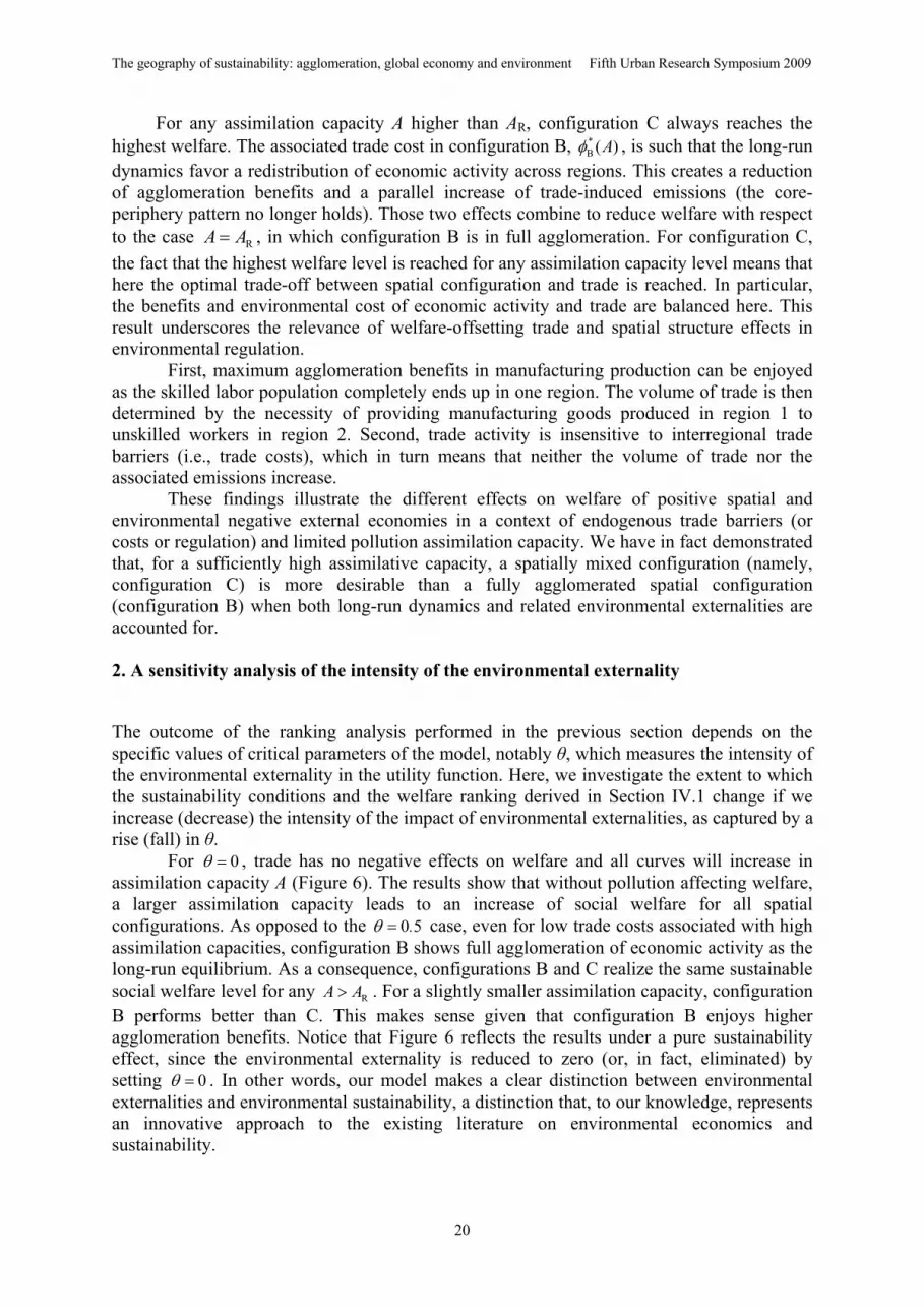
The outcome of the ranking analysis performed in the previous section depends on the specific values of critical parameters of the model, notably θ, which measures the intensity of the environmental externality in the utility function. Here, we investigate the extent to which the sustainability conditions and the welfare ranking derived in Section IV.1 change if we increase (decrease) the intensity of the impact of environmental externalities, as captured by a rise (fall) in θ. For 0θ =

0 5.

, trade has no negative effects on welfare and all curves will increase in assimilation capacity A (Figure 6). The results show that without pollution affecting welfare, a larger assimilation capacity leads to an increase of social welfare for all spatial configurations. As opposed to the θ = case, even for low trade costs associated with high assimilation capacities, configuration B shows full agglomeration of economic activity as the long-run equilibrium. As a consequence, configurations B and C realize the same sustainable social welfare level for any . For a slightly smaller assimilation capacity, configuration B performs better than C. This makes sense given that configuration B enjoys higher agglomeration benefits. Notice that Figure 6 reflects the results under a pure sustainability effect, since the environmental externality is reduced to zero (or, in fact, eliminated) by setting

RAA >

0θ = . In other words, our model makes a clear distinction between environmental externalities and environmental sustainability, a distinction that, to our knowledge, represents an innovative approach to the existing literature on environmental economics and sustainability.

20



0θ =


R

1 2 3 4AR

50%

100%

75%

0

Configuration A

Configuration B

Configuration C

FIGURE 6. WELFARE IN THE SUSTAINABLE LONG-RUN EQUILIBRIA FOR 0θ = .

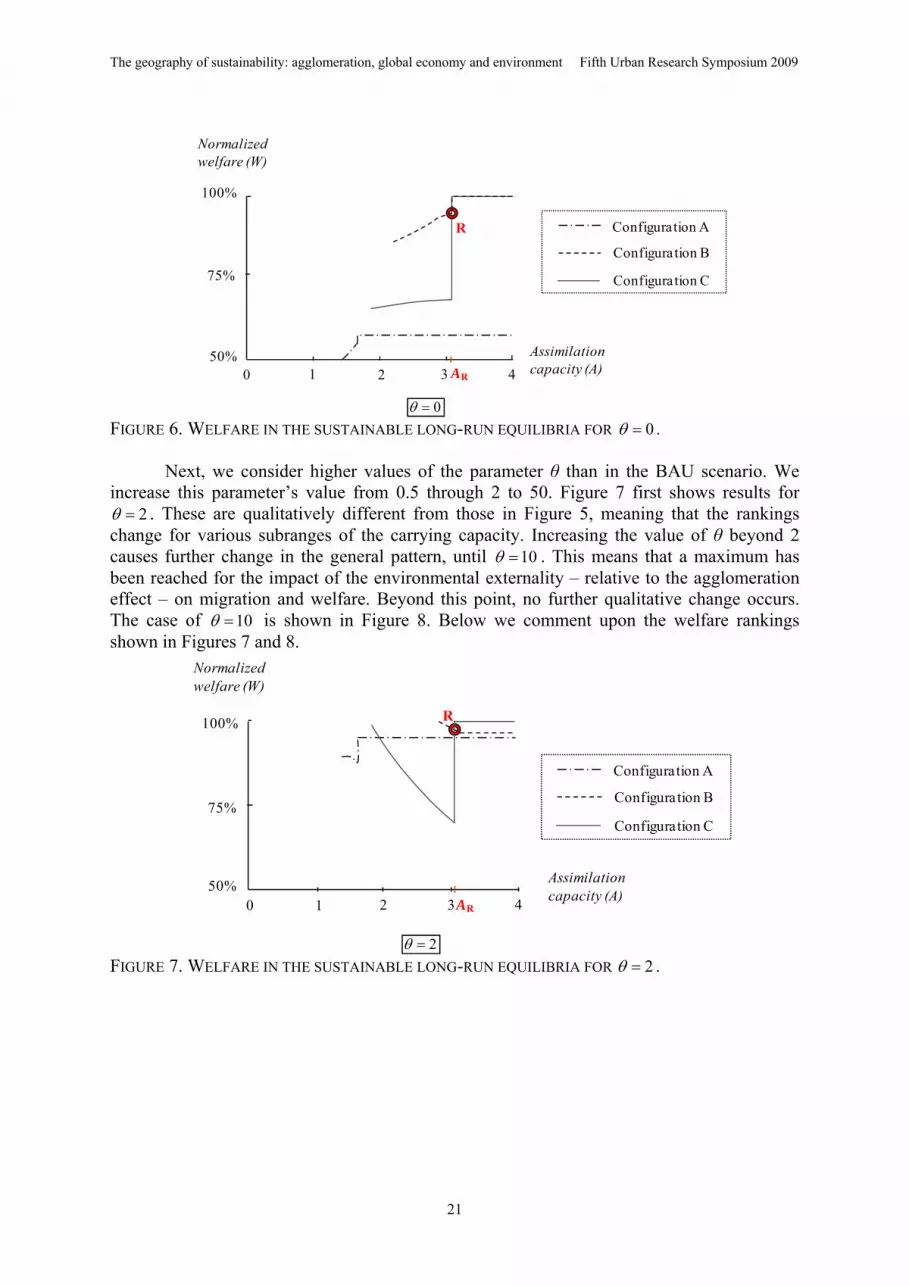
Next, we consider higher values of the parameter θ than in the BAU scenario. We increase this parameter’s value from 0.5 through 2 to 50. Figure 7 first shows results for

2θ = . These are qualitatively different from those in Figure 5, meaning that the rankings change for various subranges of the carrying capacity. Increasing the value of θ beyond 2 causes further change in the general pattern, until 10θ = . This means that a maximum has been reached for the impact of the environmental externality – relative to the agglomeration effect – on migration and welfare. Beyond this point, no further qualitative change occurs. The case of 10θ = is shown in Figure 8. Below we comment upon the welfare rankings shown in Figures 7 and 8.



R

1 2 3 450%

100%

75%

2

AR

θ =

0

Configuration A

Configuration B

Configuration C

FIGURE 7. WELFARE IN THE SUSTAINABLE LONG-RUN EQUILIBRIA FOR 2θ = .

21


Normalized welfare (W)

Assimilation capacity (A)1 2 3 4

50%

100%

75%

AR

R

0

Configuration A

Configuration B

Configuration C

10θ = FIGURE 8. WELFARE IN THE SUSTAINABLE LONG-RUN EQUILIBRIA FOR 10= . θ

Comparing figures 5, 7, and 8 reveals some consistencies and differences. The

consistencies can be summarized as follows: (i) for low values of the assimilation capacity, no spatial configuration of the economy can meet the environmental sustainability condition; (ii) for higher values of the assimilation capacity, configuration A, with low concentration of economic activity in both regions, is the only sustainable system; (iii) for even higher values of the assimilation capacity, configuration C, with a mix of low and high regional concentration of activities, is sustainable; (iv) for very high values of the assimilation capacity, all configurations are sustainable. The best-performing spatial configuration depends on the assimilation capacity and on the value of the intensity of the environmental externality θ. If its value is not too high (Figures 5 and 7) then configuration B, with both regions having concentration of activities, has the highest sustainable social welfare level. Further, beyond a threshold value of the assimilation capacity, configuration C will perform the best. The reason is that it evidently allows for the best combination of agglomeration, trade, and environmental externalities. If the intensity of the environmental externality θ attains a very high value (Figure 8), then beyond a critical threshold of the assimilation capacity, configuration A, with the lowest degree of economic concentration in both regions, reaches the highest welfare. This makes sense because the higher activity and trade levels associated with more pollution in those alternative configurations with more concentrated activities (B and C) can be regarded as being heavily punished by the high value of θ. Finally, a higher θ causes increasing declines in parts of the welfare patterns, because utility, and as a result social welfare, is more negatively influenced by a given level of environmental externality.

Next, note that, within a configuration, an increase in the assimilation capacity can cause increases or decreases in welfare, depending on what dominates: welfare benefits of extra production and trade, or welfare costs of extra environmental externalities.

V. CONCLUSIONS

This paper has developed a theoretical approach to study the impact of spatial configurations of the global economy on long-term environmental sustainability. The starting point was the notion of spatial sustainability, denoting a spatial configuration that is consistent with

22


sustainable resource use and pollution being within the assimilative capacity. We have focused here on the latter condition. Our framework accounts for three drivers of welfare and (un)sustainability, namely, agglomeration economies, advantages of trade, and environmental externalities. It extends the “footloose entrepreneur” model of the new economic geography by introducing three innovations. First, it generates different spatial configurations of the economy and transitions between these. Second, it formalizes continuously variable degrees and multi-regional heterogeneity of economic concentration in space. Third, it includes the dynamics of pollution, and distinguishes between environmental externalities and environmental sustainability.

The starting point is a spatial structure with industrial, agricultural and nature-dominated land uses. Regions are characterized by specific regional concentrations of economic activities, resulting in different intensities of agglomeration spillovers on production costs. By formalizing through a specific agglomeration-effect parameter what is known in trade theory as the “home market effect”, we capture the economic feedbacks between agglomeration patterns and the spatial structure of the economy. Through the effect of pollution on welfare differences, pollution acts as an indirect driver of migration decisions. The result is a dynamic economic theory of spatial sustainability.

The sustainability characteristics of the long-run equilibrium were studied by varying the pollution assimilation capacity, or indirectly the trade parameter, which is a core driver of spatial structure. This results in different rankings of sustainable spatial configurations in terms of global welfare. A main result of the analysis is that agglomeration of economic activities is not necessarily the most desirable spatial structure. A spatial configuration characterized by full dispersion of economic activities across regions is preferred if the intensity of environmental externalities is very high. The welfare effect of environmental externalities then outweighs that of agglomeration. For medium values of the assimilation capacity, a symmetric configuration with both regions having concentration of activities reaches the highest sustainable social welfare level. An asymmetric configuration, with one region having concentrated activities and the other having a dispersion of economic activities, performs best for higher values of assimilation capacity. In addition, for a very high intensity of the environmental externality an economy with a symmetric configuration characterized by concentrated activities is unsustainable as it generates a very high level of activity and associated emissions.

The results illustrate the relevance of welfare-offsetting spatial structure and trade effects in environmental regulation. This insight can help to formulate an effective and efficient mix of policies focusing directly on emissions reduction, redirecting trade or spatial reorganization. More specifically, the approach can be used to further investigate the interaction and complementary of such diverse instruments as pollution taxes, technological standards, land taxation, road pricing and parking tariffs. Moreover, since the approach clearly distinguishes between environmental externalities and environmental sustainability, not only it adds a dynamic element to the existing literature on trade and environment but also it can be applied to long-term environmental problems like climate change.

23


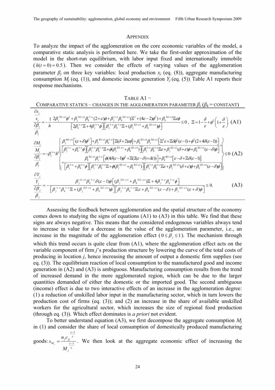
APPENDIX

To analyze the impact of the agglomeration on the core economic variables of the model, a comparative static analysis is performed here. We take the first-order approximation of the model in the short-run equilibrium, with labor input fixed and internationally immobile ( ). Then we consider the effects of varying values of the agglomeration parameter βj on three key variables: local production xj (eq. (8)), aggregate manufacturing consumption Mj (eq. (1)), and domestic income generation Yj (eq. (5)). Table A1 reports their response mechanisms.

( 0) 0.5h t = =

TABLE A1 −

COMPARATIVE STATICS – CHANGES IN THE AGGLOMERATION PARAMETER βj (βk = CONSTANT)

3(1 ) 2 2(1 ) 1 1 2(1 ) 2 2 3(1 )2

1 1 1 1 2(1 ) 2(1 )

2 (2 ) ( (4 2) )1 0 , 1 .12 4 ( )

j

j j j k j k k

j k j j k j k

j

xx

h

ε ε ε ε ε ε

ε ε ε ε ε ε

β φ β β ε φ β β ε φ β εφ δ δφβ ε εβ β φ β β β β φβ

− − − − − −

− − − − − −

∂

+ + + Ξ + − + Ξ ⎛= − ≤ Ξ = − + +⎜∂ ⎡ ⎤ ⎡ ⎤ ⎝ ⎠Ξ+ Ξ+ +⎣ ⎦ ⎣ ⎦

⎞⎟ (A1)

[ ]4(1 ) 2 3(1 ) 1 2(1 ) 2(1 ) 2 2 2

1 1 1 1 2(1 ) 2(1 ) 1 1 2(1 ) 2(1 )

1 6

( ) ( 2) ( 1) (2 4 ( 1))

( ) ( ) (j j k k j

j

j k j k j k j k j kjj

j

j

MM

h

ε ε ε ε ε

ε ε ε ε ε ε ε ε ε ε

ε

β ε δ φ β β δ εφ β β ε δφ ε φ δ ε

β β φ β β φ β β β β ε β δ ε φ β ε δβ

ββ

− − − − −

− − − − − − − − − −

−

⎡ ⎤ ⎡ ⎤+ + Ξ + + Ξ +Ξ − + + −∂ ⎣ ⎦ ⎣⎡ ⎤⎡ ⎤+ Ξ+ + Ξ + + + −⎣ ⎦⎣ ⎦=−

∂

⎦

[ ]3(1 ) 1 2 4(1 )

1 1 1 1 2(1 ) 2(1 ) 1 1 2(1 ) 2(1 )

)0

(4 ( 1) (2( ) )) ( 1)

( ) ( ) ( )k j k

j k j k j k j k j k

ε ε ε

ε ε ε ε ε ε ε ε ε ε

φ

β β φ δ ε φ ε δ δε β ε δ δ ε

β β φ β β φ β β β β ε β δ ε φ β ε δ φ

− − −

− − − − − − − − − −

⋅

+

+

⎧ ⎫⎪ ⎪

⎡ ⎤⎪ ⎪⎪ ⎣ ≤⎨ ⎬⎡ ⎤− +Ξ − + + − +Ξ −⎪ ⎪⎣ ⎦

⎪ ⎪⎡ ⎤⎡ ⎤⎡ ⎤+ Ξ+ + Ξ + + + −⎪ ⎪⎣ ⎦⎣ ⎦⎣ ⎦⎩ ⎭

⎦ ⎪ (A2)

(1 ) 1 2(1 ) 2(1 ) 1 1

1 1 2(1 ) 2(1 ) 1 1 2(1 ) 2(1 )

( 1) ( ) 40.

( ) ( ) ( )

j

j k j k j kj

j j k j k j k k j

j

YY ε ε ε ε ε ε

ε ε ε ε ε ε ε ε

β β δ ε φ β β β β φβ β β β β φ β β ε β ε δ β ε δ φβ

− − − − − −

− − − − − − − −

∂⎡ ⎤− + Ξ +⎣ ⎦= − ≤

∂ ⎡ ⎤ ⎡Ξ + + Ξ + − + +⎣ ⎦ ⎣ ⎤⎦A3) (

ssessing the feedback between agglomeration and the spatial structure of the economy

comeAs down to studying the signs of equations (A1) to (A3) in this table. We find that these

signs are always negative. This means that the considered endogenous variables always tend to increase in value for a decrease in the value of the agglomeration parameter, i.e., an increase in the magnitude of the agglomeration effect ( 0 1jβ≤ ≤ ). The mechanism through which this trend occurs is quite clear from (A1), where t meration effect acts on the variable component of firm j’s production structure by lowering the curve of the total costs of producing in location j, hence increasing the amount of output a domestic firm supplies (see eq. (3)). The equilibrium reaction of local consumption to the manufactured good and income generation in (A2) and (A3) is ambiguous. Manufacturing consumption results from the trend of increased demand in the more agglomerated region, which can be due to the larger quantities demanded of either the domestic or the imported good. The second ambiguous (income) effect is due to two interactive effects of an increase in the agglomeration degree: (1) a reduction of unskilled labor input in the manufacturing sector, which in turn lowers the production cost of firms (eq. (3)); and (2) an increase in the share of available unskilled workers for the agricultural sector, which increases the size of regional food production (through eq. (3)). Which effect dominates is a priori not evident.

To better understand equation (A3), we first decompose the

he agglo

aggregate consumption Mj in (1)

goods:

and consider the share of local consumption of domestically produced manufacturing 1

n cε

1j

j jjM

j

sM

ε

εε−= . We then look at the aggregate economic effect of increasing the

−

24


agglomeration degree in driving individual consumption choices by studying the sign of the ng equation:followi

4(1 ) 2 3(1 ) 1 2(1 ) 2(1 ) 2 2 1 3(1 ) 4(1 ) 2

1

1 1 1 1 2(1 ) 2(1 ) 1 1 2(1

( ) (2 ) (2 ) (2 ) ( )2 ( 1)jM j j k j k j k k

k

j

sh

ε ε ε ε ε ε ε ε

ε

ε ε ε ε ε ε ε ε ε

β φ ε δ β β φ ε δ β β ε φ β β φ ε δ β φ ε δβ φ ε

β β φ

− − − − − − − −

−

− − − − − − − − −

+ + Ξ + + + Ξ + Ξ − + −= − −

∂ ⎡⎣ ( )

jM

j k j k j k j k j

j

s

β β β β β φ β β ε β

β

∂

+ Ξ + + Ξ +⎤⎡ ⎤⎦⎣ ⎦) 2(1 )

0ε−

≤ (A2bis)( ) ( )kφ δ ε β φ ε δ+ + −⎡ ⎤⎣ ⎦

This share of domestic consumption of the domestically produced manufacturing good is responding negatively to an increase in the agglomeration effect of region j (i.e., a decrthe βj

value), indicating that the agglomeration effect acts in favor of the home market. This ease in

trend reflects productivity gains of firms in a more agglomerated region as a result of a decrease in the marginal production costs (eq. (A1)). These gains, in turn, benefit consumers via lower consumption prices.

To better understand equation (A3), we need to explain the aggregate economic effect of an increase in the agglomeration degree of region j on the distribution of domestic income studied in (A3). We therefore determine the shares of revenue of the industrial and agriculture sectors. By using equations (4) and (5), the share of domestic income generated

by the industrial sector is: M j

j j j j jY

j

w H n xs

Yβ+

= . We derive the effect of a marginal change in

the agglomeration on this share:

2(1 ) 1 3(1 ) 1 2(1 ) 2

14 ( 1)

M jY

jj j

sh

ε ε ε

ε ε

β φ β β φβ ε

β β

− − −

−

Ξ + Ξ= − −

∂ ⎡⎣

1 21 2(1 ) 2(1 ) 1 1 2(1 )

40.

( ) 2M jY j k k j k

k j k j k j

j

sε ε

εε ε ε ε ε

β β φβ φ β β β β β φ

β

− −−

− − − − − −

∂

Ξ +≤

⎤ ⎡ ⎤Ξ + + Ξ +⎦ ⎣ ⎦ (A3bis)

tive. Hence, our model predicts an increase in industry-relatedomestic income in response to the agglomeration of firms, which in turn raises regional

wages and domestic consumption because of the increased purchase power of consumers.16

n International Trade.” American Economic Review, 93, 1268–1290.

.”Agglomeration Effects in Europe.” European Economic Review, 46, 213-

The sign of this effect is nega d

REFERENCES

Bernard, A. B., Eaton J., Jensen B.J, and Kortum, S. (2003). “Plants and Productivity i

Ciccone, A.. 2002227.

Copeland, B. R., and Scott M. Taylor. S.M. (1995). “Trade and Transboundary Pollution.” American Economic Review, 85, 716–737.

Dixit, A. K., and. Stiglitz. J. E (1977). “Monopolistic Competition and Optimum Product Diversity.” American Economic Review, 67, 297-308.

Forslid, R., and Ottaviano. G I.P. (2003). “An Analytically Solvable Core-periphery Model.” Journal of Economic Geography, 3, 229-240.

Fujita, M. . Krugman, P, and Venables. A. J. (1999). The Spatial Economy: Cities, Regions, and International Trade. Cambridge MA, MIT Press.

Fujita, M., and Thisse, J.F. (2002). Economics of Agglomeration: Cities, Industrial Location, and Regional Growth. Cambridge, Cambridge University Press.

16 We also performed a comparative statics analysis on the effect of a change in the agglomeration parameter βj on the domestic wage wj. This turned out to be negative (results not shown here).

25





https://www.researchgate.net/publication/4901306_'Trade_and_Transboundary_Pollution'?el=1_x_8&enrichId=rgreq-8f2087d6-cbfd-4d8f-b330-8e43b5901ee5&enrichSource=Y292ZXJQYWdlOzIyODQzNDk0MztBUzoxMDI5MDQ4Nzg4NjIzNDdAMTQwMTU0NTg0Mzg1MQ==

https://www.researchgate.net/publication/4901306_'Trade_and_Transboundary_Pollution'?el=1_x_8&enrichId=rgreq-8f2087d6-cbfd-4d8f-b330-8e43b5901ee5&enrichSource=Y292ZXJQYWdlOzIyODQzNDk0MztBUzoxMDI5MDQ4Nzg4NjIzNDdAMTQwMTU0NTg0Mzg1MQ==

https://www.researchgate.net/publication/4725236_Monopolistic_Competition_and_Optimum_Product_Diversity_Reply?el=1_x_8&enrichId=rgreq-8f2087d6-cbfd-4d8f-b330-8e43b5901ee5&enrichSource=Y292ZXJQYWdlOzIyODQzNDk0MztBUzoxMDI5MDQ4Nzg4NjIzNDdAMTQwMTU0NTg0Mzg1MQ==

https://www.researchgate.net/publication/4725236_Monopolistic_Competition_and_Optimum_Product_Diversity_Reply?el=1_x_8&enrichId=rgreq-8f2087d6-cbfd-4d8f-b330-8e43b5901ee5&enrichSource=Y292ZXJQYWdlOzIyODQzNDk0MztBUzoxMDI5MDQ4Nzg4NjIzNDdAMTQwMTU0NTg0Mzg1MQ==


26

ternalities, and Trade.”

Heha, 33-54. Cambridge, Cambridge

Het Competition, and the International Economy. Cambridge, MA: MIT

Kran Economic Review, 70, 950-959.

ization for Economic Co-operation and Development.

Regional and Urban

Pe Growth: Natural

Pfld Urban Economics, 34, 565-673.

wh 62, 278-304.

Grazi, F, van den Bergh, J. C.J.M. and Rietveld. P (2007). “Spatial Welfare Economics versus Ecological Footprint: Modeling Agglomeration, ExEnvironmental and Resource Economics, 38, 135-153. lpman, E. (1998). “The Size Of Regions.” In: Topics in Public Economics. Theoretical and Empirical Analysis, ed. D. Pines, E. Sadka, and I. ZilcUniversity Press lpman, E. and Paul Krugman. 1985. Market Structure and Foreign Trade: Increasing Returns, ImperfecPress. ugman, P. (1980). “Scale Economies, Product Differentiation, and the Pattern of Trade.” Americ

Krugman, P.. (1991). “Increasing Returns and Economic Geography.” Journal of Political Economy, 99, 483-499.

OECD. 2007. 2007-2008 Programme of Work of the OECD Territorial Development Policy Committee. Paris: Organ

Ottaviano, G I.P., and Puga. D (1998). “Agglomeration in the Global Economy: a Survey of the New Economic Geography”. The World Economy, 21, 707-731.

Ottaviano, G I.P., and Jacques-François Thisse. (2004). “Agglomeration and Economic Geography.” In Henderson,V. and Thisse, J.F,editors. Handbook ofEconomics: Cities and Geography, Elsevier, Amsterdam, p 2563-2608 zzey, J.C.V., and Toman. M A. ( 2005). “Sustainability and its Economic Interpretations.” In Simpson, R.D., Toman, M.A,. Ayres R.U., editors. Scarcity andResources and the Environment in the New Millennium, RFF Press, Washington D.C., p 121-142. üger, M. (2004). “A Simple, Analytically Solvable, Chamberlinian Model.” Regional Science an

Pflüger, M. and Südekum J. (2008). “Integration, Agglomeration and Welfare.” Journal of Urban Economics, 63, 544-566.

Samuelson, P A. (1952). “The Transfer Problem and Transport Costs: The Terms of Trade en the Impediments are Absent.” Economic Journal,



https://www.researchgate.net/publication/222298362_Integration_Agglomeration_and_Welfare?el=1_x_8&enrichId=rgreq-8f2087d6-cbfd-4d8f-b330-8e43b5901ee5&enrichSource=Y292ZXJQYWdlOzIyODQzNDk0MztBUzoxMDI5MDQ4Nzg4NjIzNDdAMTQwMTU0NTg0Mzg1MQ==

https://www.researchgate.net/publication/222298362_Integration_Agglomeration_and_Welfare?el=1_x_8&enrichId=rgreq-8f2087d6-cbfd-4d8f-b330-8e43b5901ee5&enrichSource=Y292ZXJQYWdlOzIyODQzNDk0MztBUzoxMDI5MDQ4Nzg4NjIzNDdAMTQwMTU0NTg0Mzg1MQ==

Documents

The Geography of Sustainability: Agglomeration, Global Economy and Environment