arX

iv:1

411.

6215

v2 [

mat

h.A

G]

25

Nov

201

4

Suzuki-invariant codes from the Suzuki curve

Abdulla Eid, Hilaf Hasson, Amy Ksir, Justin Peachey∗

November 27, 2014

Abstract

In this paper we consider the Suzuki curve yq + y = xq0(xq + x) over the fieldwith q = 22m+1 elements. The automorphism group of this curve is known to bethe Suzuki group Sz(q) with q2(q−1)(q2+1) elements. We construct AG codes overFq4 from a Sz(q)-invariant divisor D, giving an explicit basis for the Riemann-Rochspace L(ℓD) for 0 < ℓ ≤ q2 − 1. These codes then have the full Suzuki group Sz(q)as their automorphism group. These families of codes have very good parametersand are explicitly constructed with information rate close to one. The dual codesof these families are of the same kind if 2g − 1 ≤ ℓ ≤ q2 − 1.

1 Introduction

The Suzuki curve has been a source of very good error-correcting codes. Codes con-structed from the Suzuki curve have been studied, for example, in [1], [3], [7] (one-pointcodes), and [9] (two-point codes) and shown to have very good parameters. Furthermore,the Suzuki curve has a very large automorphism group for its genus, namely the Suzukigroup Sz(q) = 2B2 of order q2(q − 1)(q2 + 1). The one-point and two-point codes pre-viously studied had automorphism groups which were not the full Suzuki group. In thispaper, we construct a family of codes on the Suzuki curve with the full Suzuki group asits group of automorphisms. We find that our codes also have very good parameters.

The outline of our paper is as follows: In Section 2 we start with some preliminariesabout the Suzuki curve. In Section 3 we give an explicit basis for the Riemann-Roch spaceL(ℓD) for 0 < ℓ ≤ q2 − 1, where the divisor D is the sum of all Fq–rational points of theSuzuki curve. In Section 4 we construct families of AG–codes with good parameters, andwith the full Suzuki group as automorphism group. These families are significant becausethey are explicitly constructed in a polynomial–time with rate close to one. In Section 5we find the dual codes of the codes constructed in Section 4 and we find the conditionsof these codes to be of the same kind, isodual, and iso–orthogonal.

The authors would like to thank Rachel Pries for organizing the workshop on rationalpoints on Suzuki Curves in which this paper was conceived.

∗This work was conducted at the Mathematics Department, Colorado State University, Summer 2011,funded by NSF grant DMS-11-01712

1

2 Preliminaries

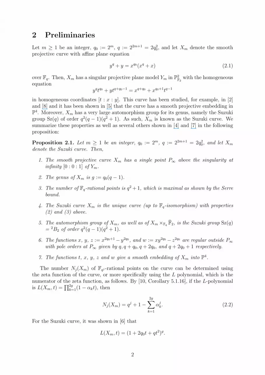
Let m ≥ 1 be an integer, q0 := 2m, q := 22m+1 = 2q20, and let Xm denote the smoothprojective curve with affine plane equation

yq + y = xq0(xq + x) (2.1)

over Fq. Then, Xm has a singular projective plane model Ym in P2

F2

with the homogeneousequation

yqtq0 + ytq+q0−1 = xq+q0 + xq0+1tq−1

in homogeneous coordinates [t : x : y]. This curve has been studied, for example, in [2]and [8] and it has been shown in [5] that the curve has a smooth projective embedding inP4. Moreover, Xm has a very large automorphism group for its genus, namely the Suzukigroup Sz(q) of order q2(q − 1)(q2 + 1). As such, Xm is known as the Suzuki curve. Wesummarize these properties as well as several others shown in [4] and [7] in the followingproposition:

Proposition 2.1. Let m ≥ 1 be an integer, q0 := 2m, q := 22m+1 = 2q20, and let Xm

denote the Suzuki curve. Then,

1. The smooth projective curve Xm has a single point P∞ above the singularity atinfinity [0 : 0 : 1] of Ym.

2. The genus of Xm is g := q0(q − 1).

3. The number of Fq-rational points is q2+1, which is maximal as shown by the Serre

bound.

4. The Suzuki curve Xm is the unique curve (up to Fq-isomorphism) with properties(2) and (3) above.

5. The automorphism group of Xm, as well as of Xm×FqF2, is the Suzuki group Sz(q)

= 2B2 of order q2(q − 1)(q2 + 1).

6. The functions x, y, z := x2q0+1− y2q0, and w := xy2q0 − z2q0 are regular outside P∞

with pole orders at P∞ given by q, q + q0, q + 2q0, and q + 2q0 + 1 respectively.

7. The functions t, x, y, z and w give a smooth embedding of Xm into P4.

The number Nj(Xm) of Fqj -rational points on the curve can be determined usingthe zeta function of the curve, or more specifically using the L polynomial, which is thenumerator of the zeta function, as follows. By [10, Corollary 5.1.16], if the L-polynomialis L(Xm, t) =

∏2g

k=1(1− αkt), then

Nj(Xm) = qj + 1−

2g∑

k=1

αjk. (2.2)

For the Suzuki curve, it was shown in [6] that

L(Xm, t) = (1 + 2q0t + qt2)g.

2

The roots of the polynomial L(Xm, t) are α, α, . . . , α︸ ︷︷ ︸

g times

and β, β, . . . , β︸ ︷︷ ︸

g times

, where

α := q0(−1 + i)

andβ := α = q0(−1− i).

Therefore,

Nj(Xm) = qj + 1− gq0(−1 + i)− gq0(−1− i) = qj + 1 + 2gq0.

In the case j = 1, we see that N1(Xm) = q + 1− q(q − 1) = q2 + 1. We will use thesepoints to construct our codes.

3 The Riemann-Roch space L(ℓD)

In order to construct an AG code whose automorphism group is the full automorphismgroup Sz(q) of Xm, we need to choose a divisor that is invariant under the action of Sz(q)on Xm. Suzuki originally constructed Sz(q) as a doubly transitive group acting on thecurve [11]. So the only way to choose an invariant divisor is to take the set of all Fqj

points for some j. The smallest such set of points is the set of Fq-points.Consider the divisor D ∈ Div(Xm) given by the sum of all Fq-rational points of Xm.

These are the points Pα,β with affine coordinates (α, β) for any α and β in Fq, plus thepoint at infinity. Thus

D = P∞ +∑

α,β∈Fq

Pα,β.

Since there are q2 + 1 many Fq-rational points of Xm, deg(D) = q2 + 1. Moreover, thedivisor D is fixed by Sz(q), so codes based at D will have Sz(q) as their automorphismgroup. In this section, we prove the following theorem, finding an explicit Fq-basis forthe space L(ℓD), where ℓ ≤ q2 − 1.

Theorem 3.1. Let ℓ ∈ N, ℓ ≤ q2 − 1, and D be defined to be the sum of all Fq-rationalpoints of Xm. Then,

S :=

xaybzcwd

(xq + x)r:aq + b(q + q0) + c(q + 2q0) + d(q + 2q0 + 1) ≤ rq2 + ℓ,0 ≤ a ≤ q − 1, 0 ≤ b ≤ 1, 0 ≤ c ≤ q0 − 1,0 ≤ d ≤ q0 − 1, 0 ≤ r ≤ ℓ

(3.1)

is a basis for L(ℓD).

Note that the function xq + x vanishes at every affine point of Xm and has a pole oforder q2 at P∞. Therefore

div(xq + x) = −q2P∞ +∑

α,β∈Fq

Pα,β.

Hence, ℓD = ℓ(q2 + 1)P∞ + div((xq + x)ℓ), i.e., ℓD ∼ ℓ(q2 + 1)P∞. Thus, we havethat L(ℓD) ≃ L(ℓ(q2 + 1)P∞) where the Fq-isomorphism is given by f 7→ f(xq + x)ℓ forf ∈ L(ℓD). Thus Theorem 3.1 is equivalent (via rnew = ℓ− rold) to the following.

3

Theorem 3.2. Let ℓ ∈ N, ℓ ≤ q2 − 1. Then

S ′ :=

xaybzcwd(xq + x)r :

aq + b(q + q0) + c(q + 2q0) + d(q + 2q0 + 1) + rq2 ≤ ℓ(q2 + 1)0 ≤ a ≤ q − 1, 0 ≤ b ≤ 1, 0 ≤ c ≤ q0 − 1,0 ≤ d ≤ q0 − 1, 0 ≤ r ≤ ℓ

(3.2)is a basis for L(ℓ(q2 + 1)P∞).

In order to prove this theorem, we recall a result in [7]. Let P ⊆ Z≥0 be the semigroupgenerated by the pole orders of the functions x, y, z, and w defined in Proposition 2.1.That is,

P := 〈q, q + q0, q + 2q0, q + 2q0 + 1〉 ⊆ Z≥0. (3.3)

Proposition 1.6 in [7] is equivalent to the following:

Proposition 3.3. ([7]) For every integer j,

dimFq(L(jP∞)) = #{n ∈ P|n ≤ j}.

We are now ready for the proof.

Proof. (Theorem 3.2) Let f = xaybzcwd(xq + x)r be an element of S ′, and let v∞ be thediscrete valuation corresponding to the point P∞. Then

v∞(f) = −[aq + b(q + q0) + c(q + 2q0) + d(q + 2q0 + 1) + rq2

],

and f has no other poles. Thus the first inequality in the definition of S ′ shows thatS ′ ⊆ L(ℓ(q2 + 1)P∞). Thus, in light of Proposition 3.3, it suffices to show that for everyn ∈ P such that n ≤ ℓ(q2 +1), S ′ contains exactly one function with a pole of order n atP∞. First we show that the valuations at P∞ of the functions in S ′ are distinct. Supposethat F1 and F2 in S ′ had the same valuation at infinity, where F1 = xa1yb1zc1wd1(xq+x)r1

and F2 = xa2yb2zc2wd2(xq + x)r2 . Then

a1q + b1(q + q0) + c1(q + 2q0) + d1(q + 2q0 + 1) + r1q2 =

a2q + b2(q + q0) + c2(q + 2q0) + d2(q + 2q0 + 1) + r2q2. (3.4)

We consider (3.4) modulo q0. Then,

d1 ≡ d2 (mod q0).

Since 1 ≤ d1, d2 ≤ q0 − 1, it must be that d1 = d2.Next, we consider (3.4) modulo 2q0. Then,

b1q0 + d1 ≡ b2q0 + d1 (mod 2q0).

Note that 0 ≤ b1, b2 ≤ 1. Thus, is must be that b1 = b2.Next, consider (3.4) modulo q. Since d1 = d2 and b1 = b2, we get

2c1q0 ≡ 2c2q0 (mod q)

and therefore c1 ≡ c2 (mod q0). Since 0 ≤ c1, c2 ≤ q0−1, it must be the case that c1 = c2.Finally, consider (3.4) modulo q2. Then, since b1 = b2, c1 = c2, d1 = d2, we have

a1q ≡ a2q (mod q2).

4

Note that 0 ≤ a1, a2 ≤ q−1. Thus, it must be that a1 = a2. This also shows that r1 = r2.We conclude that if v∞(F1) = v∞(F2), then F1 = F2.

Now we must show that if n ≤ ℓ(q2 + 1) is an element of P, then there is a functionin S ′ with pole order n at P∞. Let n be such an element. By definition,

n = aq + b(q + q0) + c(q + 2q0) + d(q + 2q0 + 1) (3.5)

for some positive integers a, b, c, d. We need to show that there are a′,b′,c′,d′, and r suchthat

n = a′q + b′(q + q0) + c′(q + 2q0) + d′(q + 2q0 + 1) + rq2 (3.6)

and 0 ≤ a′ ≤ q − 1, 0 ≤ b′ ≤ 1, 0 ≤ c′ ≤ q0 − 1, 0 ≤ d′ ≤ q0 − 1, and 0 ≤ r ≤ ℓ.Let d′ be the remainder when n is divided by q0. Then d′ will be in the correct range.

Let

nd =n− d′(q + 2q0 + 1)

q0.

Let b′ be the remainder when nd is divided by 2. Again, b′ will be in the correct range.Let

nb =nd − b′(2q0 + 1)

2.

Let c′ be the remainder when nb is divided by q0. Now 0 ≤ c′ ≤ q0 − 1. Let

nc =nb − c′(q0 + 1)

q0.

Finally, let a′ be the remainder when nc is divided by q, so that 0 ≤ a′ ≤ q − 1, and let

r =nc − a′

q.

Then we can put these back together as follows:

n = ndq0 + d′(q + 2q0 + 1)

= (2nb + b′(2q0 + 1))q0 + d′(q + 2q0 + 1)

= 2q0nb + b′(q + q0) + d′(q + 2q0 + q)

= 2q0(q0nc + c′(q0 + 1)) + b′(q + q0) + d′(q + 2q0 + q)

= ncq + c′(q + 2q0) + b′(q + q0) + d′(q + 2q0 + q)

= rq2 + a′q + c′(q + 2q0) + b′(q + q0) + d′(q + 2q0 + q).

What remains is to show that r is in the correct range. Since n ≤ ℓ(q2 + 1), this meansthat

nd ≤ ℓ(2qq0 +1

q0)

nb ≤ ℓ(qq0 +1

2q0)

nc ≤ ℓ(q +1

q)

r ≤ ℓ +ℓ

q2.

5

Since r is an integer and ℓ < q2, this means that r ≤ ℓ. Finally, to see that 0 ≤ r weneed first to show that nd, nb, nc are positive integers. Since n ≡ d′ (mod q0), we havethat d ≡ d′ (mod q0) and so we can write d− d′ = tdq0, for some positive integer td (notethe previous assumtion asserts that d ≥ d′, otherwise we have d already in the requiredrange and we don’t need to find nd). Now we have that

nd : =n− d′(q + 2q0 + 1)

q0=

aq + b(q + q0) + c(q + 2q0) + (d− d′)(q + 2q0 + 1)

q0= a(2q0) + b(2q0 + 1) + c(2q0 + 2) + td(q + 2q0 + 1)

which is a positive integer.Next we have that nd ≡ b′ (mod 2), so we have b + td ≡ b′ (mod 2) and so again we

can write it as b+ tb − b′ = 2tb, for some positive integer tb ( with the same assumptionas before that b is not in the required range {0, 1}, so b ≥ b′). Now we have that

nb : =nd − b′(2q0 + 1)

2=

a(2q0 + c(2q0 + 2) + (b+ td − b′)(2q0 + 1) + td(q)

2= a(q0) + c(q0 + 1) + tb(2q0 + 1) + tdq

20

Which is again a positive integer.Next, we have that nb ≡ c′ (mod q0), so we have c + tb ≡ c′ (mod q)0 and we write

c+ tb − c′ = tcq0, for some positive integer tc and we have that

nc : =nb − c′(q0 + 1)

q0=

a(q0) + (c+ tb − c′)(q0 + 1) + tbq0 + tdq20

q0= a + tc(q0 + 1) + tb + tdq0

which is a positive integer. Finally, we have nc ≡ a′ (mod q) and so we have nc − a′ ismultiple of q and thus r is a positive integer.

Remark 1. The dimension of L(ℓD) is given by

dimFqL(ℓD) = ℓ(q2 + 1)− q0(q − 1) + 1, (3.7)

which we can see in two ways. First, since q2 + 1 > 2q0(q − 1), we have degD > 2gand the result follows from the Riemann-Roch theorem. Second, in [7, Appendix A], itis shown that #(N \P) = q0(q− 1), and an analysis of their proof shows that the largestnumber in N \ P is 2q0(q − 1)− 1. Thus #S is the number of possibilities for a, b, c, d,and r, minus #(N \ P).

Theorem 3.1 gives us an explicit basis for L(ℓD), which we use to construct Suzuki-invariant codes in the next section.

4 Construction and properties of the code C(E, ℓD)

As above, let D ∈ Div(Xm) be the sum of all Fq-rational points in Xm. By Theorem 3.1,for ℓ ≤ q2 − 1 the Riemann-Roch space L(ℓD) has the Fq-basis (3.1), and by Remark 1dimFq

L(ℓD) = ℓ(q2 + 1)− g + 1 = ℓ(q2 + 1)− q0(q − 1) + 1.

6

Now to construct a Suzuki-invariant geometry code, we must choose another set ofpoints, disjoint from D, which is also invariant under Sz(q). Since we have used all ofthe Fq points for D, we must look to points over extensions of Fq. Consider the fieldextension Fq4 of Fq. Let the divisor E ∈ Div(Xm) be the sum of all Fq4-points minus thesum of all Fq-points. Then, we have

n := deg(E) = N4(Xm)−N1(Xm),

where N4(Xm) is given by the formula (2.2), i.e.,

N4(Xm) = q4 + 1− g(α4 + β4) = q4 + 1 + 2gq2 = q4 + 1 + 2q0q2(q − 1).

Therefore, n = deg(E) = q4 + 1 + 2q0q2(q − 1)− (q2 + 1) = q4 + 2q0q

2(q − 1)− q2.Since Supp(E)∩Supp(D) = ∅ and Theorem 3.1 provides an explicit basis for L(ℓD),

we construct an algebraic geometry code using the divisors E,D as follows. Let P1, . . . , Pn

be all the points in support of E. Define

Cm,ℓ := CL(E, ℓ ·D) = {(f(P1), f(P2), . . . , f(Pn)) ∈ Fnq4 | f ∈ L(ℓ ·D)}.

Then, we have the following theorem.

Theorem 4.1. Consider the algebraic geometry code

Cm,ℓ := CL(E, ℓ ·D)

over Fq4, where ℓ ≤ q2 − 1. Then, Cm,ℓ is an [n, k, d]-linear code, where

n = deg(E) = q4 + 2q0q2(q − 1)− q2,

k := dimFqL(ℓ ·D) = ℓ(q2 + 1)− q0(q − 1) + 1,

d ≥ d∗ := n− deg(ℓ ·D) = n− ℓ(q2 + 1).

Moreover, this code can correct at least t = ⌊(d∗ − 1)/2⌋ errors, and has Sz(q) as itsautomorphism group.

Remark 2. Let S = {f1, . . . , fk} be the Fq-basis for L(ℓD) as in Theorem 3.1. Then,the code Cm,ℓ has generator matrix Gm,ℓ := (fj(Pi))1≤j≤k,1≤i≤n.

Proof. The parameters n and k were computed above; d, d∗ and t come from the generaltheory of AG codes. Because we chose D to be an invariant divisor, the code will havethe full group Sz(q) as its automorphism group.

Remark 3. It is easy to check, using equation (2.2), that the number of points of Xm

over Fq2 and Fq3 are

N2(Xm) = q2 + 1; N3(Xm) = q3 + 1− q2(q − 1) = q2 + 1.

Thus if we let Ej be the sum of all Fqj -points minus the sum of all Fq-points, thendeg(E2) = deg(E3) = 0. Therefore E4, which is the E we used above, is the first non-trivial case.

In fact, the Suzuki curve is a maximal curve over Fq4 , meeting the Hasse-Weil bound.

7

We now focus on the family of codes where ℓ = q2−1. Denote this family by Cm, i.e.,Cm := Cm,q2−1 = CL(E, (q2 − 1)D). By Theorem 4.1, Cm is a [n, k, d ≥ d∗]-linear code,where

n = q4 + 2q0q2(q − 1)− q2,

k = (q2 − 1)(q2 + 1)− q0(q − 1) + 1 = q4 − q0(q − 1),

d∗ = n− q4 + 1 = 2q0q2(q − 1)− q2 + 1.

Using the above, Cm has information rate

Rm :=kmnm

=q4 − q0q + q0

q4 + 2q0q2(q − 1)− q2=

16q80 − 2q30 + q016q80 + 16q70 − 4q50 − 4q40

.

Thus, as m → ∞, we have Rm → 1. This shows that these codes are siginficant becausethey have very good parameter, explicitly constructed in polynomial–time, with rateasymptotically approaches one, and in many cases cannot be achieved by Reed–Solomoncodes.

Example 4.2. The rate gets close to one very quickly. In order to show this, let usconsider the following examples:

1. Let m = 1; thus, q = 8, q0 = 2. Then, the resulting code C1 = C1,63 is a[5824, 4082,≥ 1729]-linear code over F4096 and can correct up to 864 errors withinformation rate R1 = 0.7008.

2. Let m = 2; thus, q = 25 = 32, q0 = 4. Then, the resulting code C2 = C2,1023 is a[1051679, 1048452,≥ 3104]-linear code over F1048576 and can correct at least 1551errors with information rate R2 = 0.996.

5 Dual code

As before, let D be the sum of all Fq-points and the divisor E is the sum of all Fq4-rational points minus all the Fq-rational points. Next, we study the dual code of the codeCm,ℓ := CL(E, ℓD), where ℓ ≤ q2 − 1.

Recall from [10, Proposition 2.2.10] that the dual of an algebraic geometry code isgiven by CL(E, ℓD)⊥ = CL(E,E − ℓD + (η)) , where η is a Weil differential such thatνPi

(η) = −1 and resPi(η) = 1, for all i = 1, 2, . . . , n.

In order to find η we first identify the points of P1Fq4

whose fiber in Xm via the map

induced by x has an Fq4-rational point. By Proposition 2.1, P∞ is the unique point aboveinfinity.

We therefore focus on the points that lie in the affine patch of Xm isomorphic to theopen affine t 6= 0 of the model Ym. Note that y

q+ y−αq0(αq +α) factors completely intolinear terms over Fq4 for exactly q3 + 2gq many α’s in Fq4 , and that for the rest of theα’s the polynomial factors into q/2 many irreducible components, each of degree 2. ByKummer’s criterion [10, Theorem 3.3.7] applied to the equation yq+y−xq0(xq+x) = 0, thisimplies that there are exactly q3 + 2gq many Fq4-rational points of A

1Fq4

that completely

split in Xm, whereas the rest of Fq4-rational points of A1Fq4

don’t have an Fq4-rational

point in their fiber.

8

Let T be the set of α’s in Fq4 such that x = α splits, and let t :=∏

α∈T (x − α) beviewed as an element of the function field κ(Xm) of Xm, and let η := dt/t.

By the above discussion, every Fq4-rational point P of Xm except for P∞ lies abovesome affine point Qα := (x− α) of P1

Fq4

where α ∈ T . Therefore:

vP (t) = e(P |Qα)vQα(t) = 1 · vQα

(∏

α∈T

(x− α)) = 1.

And so:

vP (η) = vP (dt/t) = −1

and

resP (η) = resP (1/t) = 1

Therefore η satisfies the conditions of Proposition 2.2.10 in [10]. We will now compute(η). Note that t has zeros at all the Fq4-rational places except at P∞, that is,

(t)0 = E +D − P∞.

Let Q∞ denote the point at infinity of P1Fq4. Then:

vP∞(t) = vP∞

(∏

α∈T

(x− α)) = e(P∞|Q∞)vQ∞(∏

α∈T

(x− α)) = −q|T | = −q(q3 + 2gq)

= −q4 − 2gq2.

Therefore (t)∞ = (q4 + 2gq2)P∞. Therefore,

(t) = (t)0 − (t)∞ = E +D − P∞ − (q4 + 2gq2)P∞.

It follows that (η) = (dt/t) = (2g − 2)P∞ − E −D + P∞ + (q4 + 2gq2)P∞. Thus, by[10, Proposition 2.2.10], the dual of Cm,ℓ = CL(E, ℓD) is given by CL(E,G⊥), where

G⊥ = E − ℓD + (η)

= E − ℓD + (2g − 2)P∞ −E −D + P∞ + (q4 + 2gq2)P∞

= (−1− ℓ)D + (2g − 2 + 1 + q4 + 2gq2)P∞

= (−1− ℓ)D + (q2 − 1 + 2g)(q2 + 1)P∞.

Since D ∼ (q2 + 1)P∞,

G⊥ ∼ (−1− ℓ)D + (q2 + 2g − 1)D

∼ (q2 + 2g − 1− 1− ℓ)D.

Thus, the dual code of CL(E, ℓD) is equivalent to the code CL(E, (q2+2g−2− ℓ)D).Moreover, the dual code CL(E, (q2+2g−2−ℓ)D) is also of the form Cm,ℓ′ = CL(E, ℓ′D)

if q2 + 2g − 2 − ℓ ≤ q2 − 1, i.e., whenever 2g − 1 ≤ ℓ ≤ q2 − 1. (In which caseℓ′ = q2 + 2g − 2− ℓ.)

Thus, we obtain the following result.

9

Proposition 5.1. If ℓ ≤ q2−1, then the dual code of CL(E, ℓD) is equivalent to the codeCL(E, (−1 − ℓ + q2 + 2g − 1)D). Moreover, if 2g − 1 ≤ ℓ, C⊥

m,ℓ is of the form Cm,ℓ′ forℓ′ = q2 + 2g − 2− ℓ.

Remark 4. The code CL(E, ℓD) is isodual if and only if for the Weil differential above,we have

2ℓD − E = (η)

2ℓD − E = (2g − 2)P∞ − E −D + P∞ + (q4 + 2gq2)P∞

2ℓD = (q4 + 2gq2 + 2g − 1)P∞ −D

2ℓD ∼ (q2 + 2g − 1)D −D

2ℓ = q2 + 2g − 2

ℓ =q2

2+ g − 1.

Hence, we have:

1. CL(E, ℓD) is isodual if and only if ℓ = q2/2 + g − 1.

2. CL(E, ℓD) is iso-orthogonal if and only if ℓ ≤ q2/2 + g − 1.

Example 5.2. The smallest case of an isodual code in our family is the case m = 1 andℓ = q2/2 + g − 1 = 82/2 + 14− 1 = 45. In that case the code C1,45 is isodual.

Remark 5. Note that since the codes CL(E, ℓD) and CL(E, ℓ(q2+1)P∞) are equivalent(since D ∼ (q2 + 1)P∞), the code Cm,ℓ is a one-point algebraic geometry code.

References

[1] Chen, C., Duursma, I.: Geometry Reed-Solomon codes of length 64 and 65 over F8.IEEE Transactions in Information Theory 49 no. 5, 1351-1353 (2003)

[2] Deligne P., Lusztig G.: Representations of reductive groups over finite fields. Ann.of Math. 103, 103–161 (1976)

[3] Duursma, I., Park S.: Delta sets for divisors supported in two points. Finite FieldsAppl. 18 no. 5, 865–885 (2012)

[4] Fuhrmann R., Fernando T.: On Weierstrass points and optimal curves. Rend. Circ.Mat. Palermo (2) Suppl. no. 51, 25–46 (1998)

[5] Giulietti M., Korchmaros G., Torres F.: Quotient curves of the Suzuki curve. ActaArith. 122. no. 3, 245–274 (2006)

[6] Hansen J. P.: Deligne-Lusztig varieties and group codes. Coding theory and al-gebraic geometry (Luminy, 1991), 63–81. Lecture Notes in Math. 1518. Springer,Berlin (1992)

[7] Hansen J. P., Stichtenoth H.: Group codes on certain algebraic curves with manyrational points. Appl. Algebra Engrg. Comm. Comput. 1. no. 1, 67–77 (1990)

10

[8] Henn, H.: Funktionenkorper mit grosser Automorphismengruppe. J. Reine Angew.Math. 302, 96–115 (1978)

[9] Matthews, G.L: Codes from the Suzuki function field. IEEE Trans. Inform. Theory50. no. 12, 3298–3302 (2004)

[10] Stichtenoth, H.: Algebraic function field and code. Springer, Berlin (2009)

[11] Suzuki, M.: On a class of doubly transitive groups. Ann. of Math. 75, 105–145(1962)

Current authors information:Abdulla Eid: Department of Mathematics at BTC, University of Bahrain, Bahrainemail: aeid@uob.edu.bh

Hilaf Hasson: Department of Mathematics, Stanford University, Palo Alto, CA 94305,USAemail: hilaf@stanford.edu

Amy Ksir: Department of Mathematics, United States Naval Academy, Annapolis, MD21402, USAemail: ksir@usna.edu

Justin Peachey: Independent Researcheremail: jdpeachey@gmail.com

11