Embed Size (px)
Citation preview
AIMS Mathematics, 6(7): 7798‒7832.
DOI: 10.3934/math.2021454
Received: 16 February 2021
Accepted: 11 May 2021
Published: 17 May 2021
http://www.aimspress.com/journal/Math
Research article
Some average aggregation operators based on spherical fuzzy soft sets
and their applications in multi-criteria decision making
Jabbar Ahmmad1, Tahir Mahmood1, Ronnason Chinram2,* and Aiyared Iampan3
1 Department of Mathematics and Statistics, International Islamic University, Islamabad 44000, Pakistan
2 Algebra and Applications Research Unit, Division of Computational Science, Faculty of Science, Prince of Songkla University, Hat Yai, Songkhla 90110, Thailand
3 Department of Mathematics, School of Science, University of Phayao, Phayao 56000, Thailand
* Correspondence: Email: [email protected].
Abstract: Spherical fuzzy soft sets 𝑆𝐹𝑆 𝑆𝑠 have its importance in a situation where human opinion is not only restricted to yes or no but some kind of abstinence or refusal aspects are also involved. Moreover, the notion of 𝑆𝐹𝑆 𝑆 is free from all that complexities which suffers the contemporary theories because parameterization toll is a more important character of 𝑆𝐹𝑆 𝑆. Also, note that aggregation operators are very effective apparatus to convert the overall information into a single value which further helps in decision-making problems. Due to these reasons, based on a spherical fuzzy soft set 𝑆𝐹𝑆 𝑆 , we have first introduced basic operational laws and then based on these introduced operational laws, some new notions like spherical fuzzy soft weighted average
𝑆𝐹𝑆 𝑊𝐴 aggregation operator, spherical fuzzy soft ordered weighted average 𝑆𝐹𝑆 𝑂𝑊𝐴 aggregation operator and spherical fuzzy soft hybrid average 𝑆𝐹𝑆 𝐻𝐴 aggregation
operators are introduced. Furthermore, the properties of these aggregation operators are discussed in detail. An algorithm is established in the environment of 𝑆𝐹𝑆 𝑆 and a numerical example are given to show the authenticity of the introduced work. Moreover, a comparative study is established with other existing methods to show the validity and superiority of the established work.
Keywords: spherical fuzzy set; spherical fuzzy soft set; aggregation operators; multicriteria decision making Mathematics Subject Classification: 03E72, 62C86
7799
AIMS Mathematics Volume 6, Issue 7, 7798–7832.
1. Introduction
Fuzzy set (FS) proposed by Zadeh [1] established the foundation in the field of fuzzy set theory and provided a track to address the difficulties of acquiring accurate data for multi-attribute decision-making problems. Fuzzy set only considers membership grade (MG) "𝔞" which is bounded to 0, 1 ] while in many real-life problems we have to deal with not only MG but also non-membership grade (NMG) "𝔟", and due to this reason, the concept of FS has been extended to intuitionistic fuzzy set (IFS) established by Atanassov [2] that also compensate the drawback of FS. IFS has gained the attention of many researchers and they have used it for their desired results in practical examples for decision-making problems. IFS also enlarges the information space for decision-makers (DMs) because NMG is also involved with the condition that 0 𝔞 𝔟 1. Zhao et al. [3] established the generalized intuitionistic fuzzy aggregation operators. Moreover, some intuitionistic fuzzy weighted average, intuitionistic fuzzy ordered weighted average, and intuitionistic fuzzy hybrid average aggregation operators are introduced in [4]. Moreover, IF interaction aggregation operators and IF hybrid arithmetic and geometric aggregation operators are established in [5]. Later on, the MG and NMG are denoted by interval values and a new notion has been introduced called interval-valued IFS (IVIFS) [6] being a generalization of FS and IFS. The notions of IFS and IVIFS have been applied to many areas like group decision-making [7], similarity measure [8], and multicriteria decision-making problems [9]. Zhang et al. [10] introduce some information measures for interval-valued intuitionistic fuzzy sets. In many decision-making problems when decision-makers prove 0.6 as an MG and "0.5" as NMG then IFS fail to handle this kind of information, so to overcome this issue, the idea of IFS is further extended to the Pythagorean fuzzy set 𝑃 𝐹𝑆 established by Yager [11] with condition that 0 𝔞 𝔟 1. Therefore, 𝑃 𝐹𝑆 can express more information and IFS can be viewed as a particular case of 𝑃 𝐹𝑆. Since aggregation operators are very helpful to change the overall data into single value which help us in decision-making problems for the selection of the best alternative among the given ones, so Khan et al. [12] introduced Pythagorean fuzzy Dombi aggregation operators and their application in decision support system. Moreover, 𝑃 𝐹 interaction aggregation operators and their application to multiple-attribute decision-making have been proposed in [13]. In many circumstances, we have information that cannot be tackled by 𝑃 𝐹𝑆 like 𝑠𝑢𝑚 0.8 , 0.9 ∉ 0, 1 , to compensate for this hurdle the idea of .q-rung orthopair fuzzy set (q-ROFS) is established by Yager [14] with condition that 0 𝔞 𝔟 1 for 𝑞 1. It is clear that IFS and 𝑃 𝐹𝑆 are special cases of q-ROFS and it is more strong apparatus to deal with the fuzzy information more accurately. Wei et al. [15] introduced some q‐rung orthopair fuzzy Heronian mean operators in multiple attribute decision making. Moreover, Liu and Wang [16] established the multiple-attribute decision-making based on Archimedean Bonferroni operators. Since all ideas given above can only consider only MG and NMG, while in many decision-making problems we need to consider the abstinence grade (AG) "𝔠", hence to overcome this drawback, the idea of picture fuzzy set (PFS) has been introduced by Cuong [17]. Cuong et al. [18] introduce the primary fuzzy logic operators, conjunction, disjunction, negation, and implication based on PFS. Furthermore, some concepts and operational laws are proposed by Wang et al. [19], and also some picture fuzzy geometric aggregation operators and their properties have been discussed by them. Some PF aggregation operators are also discussed in [20,21]. Zeng et al. [22] introduced the extended version of the linguistic picture fuzzy Topsis method and its application in enterprise resource planning systems. In the picture fuzzy set, we have a condition that 0 𝔞 𝔟 𝔠 1, but in many decision-making problems, the information given by experts cannot be handled by PFS and PFS fail to hold. For example, when experts provide "0.6" as MG, "0.5" as
7800
AIMS Mathematics Volume 6, Issue 7, 7798–7832.
NMG, and "0.3" as AG then we can see that 𝑠𝑢𝑚 0.6, 0.5, 0.3 ∉ 0, 1 . To overcome this difficulty, the idea of a spherical fuzzy set has been proposed by Mahmood et al. [23] with condition that 0 𝔞 𝔟 𝔠 1 . So, SFS is a more general form and provides more space to decision-makers for making their decision in many multi-attribute group decision-making problems. Jin et al. [24] discover the spherical fuzzy logarithmic aggregation operators based on entropy and their application in decision support systems. Furthermore, some weighted average, weighted geometric, and Harmonic mean aggregation operators based on the SF environment with their application in group decision-making problems have been discussed in [25,26]. Also, some spherical fuzzy Dombi aggregation operators are defined in [27]. Ashraf et al. [28] introduced the GRA method based on a spherical linguistic fuzzy Choquet integral environment. Ali et al. [29] introduced the TOPSIS method based on a complex spherical fuzzy set with Bonferroni mean operator.
Note that all the above existing literature has the characteristic that they can only deal with fuzzy information and cannot consider the parameterization structure. Due to this reason, Molodtsov [30] introduced the idea of a soft set (SS) which is more general than that of FS due to parameterization structure. Moreover, Maji et al. [31,32] use the SS in multi-criteria decision-making problems. The notions of a fuzzy soft set 𝐹𝑆 𝑆 has been introduced by Maji et al. [33] which is the combination of fuzzy set and soft set. Also, the applications of 𝐹𝑆 𝑆 theory to BCK/BC-algebra, in medical diagnosis, and decision-making problems have been established in [34–36]. Similarly as FS set is generalized into IFS, 𝐹𝑆 𝑆 is generalized into an intuitionistic fuzzy soft set 𝐼𝐹𝑆 𝑆 [37] that is more strong apparatus to deal with fuzzy soft theory. Furthermore, Garg and Arora [38] introduced Bonferroni mean aggregation operators under an intuitionistic fuzzy soft set environment and proposed their applications to decision-making problems. Moreover, the concept of intuitionistic fuzzy parameterized soft set theory and its application in decision-making have been established in [39]. Since 𝐼𝐹𝑆 𝑆 is a limited notion, so the idea of Pythagorean fuzzy soft set 𝑃 𝐹𝑆 𝑆 has been established by Peng et al. [40]. Furthermore q-rung orthopair fuzzy soft set generalizes the intuitionistic fuzzy soft set, as well as the Pythagorean fuzzy soft set and some q-rung orthopair fuzzy soft aggregation operators, are defined by Husain et al. [41]. Since 𝐹𝑆 𝑆, 𝐼𝐹𝑆 𝑆, 𝑃 𝐹𝑆 𝑆 and 𝑞 𝑅𝑂𝐹𝑆 𝑆 can only explore the MG and NMG but they cannot consider the AG, so to overcome this drawback, PFS and SS are combined to introduce a more general notion called picture fuzzy soft set 𝑃𝐹𝑆 𝑆 given in [42]. Also, Jan et al. [43] introduced the multi-valued picture fuzzy soft sets and discussed their applications in group decision-making problems. Furthermore, SFS and soft set are combined to introduce a new notion called spherical fuzzy soft set 𝑆𝐹𝑆 𝑆 discussed in [44] being the generalization of picture fuzzy soft set. Furthermore, the concepts of interval-valued neutrosophic fuzzy soft set and bipolar fuzzy neutrosophic fuzzy soft set along with their application in decision-making problems have been introduced in [45,46].
The motivation of the study is to use 𝑆𝐹𝑆 𝑆 because (1) Most of the existing structure like 𝐹𝑆 𝑆, 𝐼𝐹𝑆 𝑆, 𝑃 𝐹𝑆 𝑆, 𝑞 𝑅𝑂𝐹𝑆 𝑆 and 𝑃𝐹𝑆 𝑆 are the special cases of 𝑆𝐹𝑆 𝑆. (2) Also, note that 𝑆𝐹𝑆 𝑆 can cope with the information involving the human opinion based on MG, AG, NMG, and RG. Consider the example of voting where one can vote in favor of someone or vote against someone or abstain to vote or refuse to vote. 𝑆𝐹𝑆 𝑆 can easily handle this situation, while the existing structures like 𝐹𝑆 𝑆, 𝐼𝐹𝑆 𝑆, 𝑃 𝐹𝑆 𝑆 and 𝑞 𝑅𝑂𝐹𝑆 𝑆 can note cope this situation due to lack of AG or RG. (3) The aim of using 𝑆𝐹𝑆 𝑆 is to enhance the space of 𝑃𝐹𝑆 𝑆 because 𝑃𝐹𝑆 𝑆 has its limitation in assigning MG, AG, and NMG to the element of a set. (4) Also note that FS, IFS, 𝑃 𝐹𝑆 and q-ROFS are non-parameterized structure, while 𝑆𝐹𝑆 𝑆 is a parameterized
7801
AIMS Mathematics Volume 6, Issue 7, 7798–7832.
structure, so 𝑆𝐹𝑆 𝑆 has more advantages over all these concepts. So in this article, based on 𝑆𝐹𝑆 𝑆, we have introduced the idea of 𝑆𝐹𝑆 𝑊𝐴, 𝑆𝐹𝑆 𝑂𝑊𝐴 and 𝑆𝐹𝑆 𝐻𝐴 aggregation operators. Moreover, their properties are discussed in detail.
Further, we organize our article as follows: Section 2 deal with basic notions of FS, 𝑆 𝑆, PFS, 𝑃𝐹𝑆 𝑆, SFS and 𝑆𝐹𝑆 𝑆 and their operational laws. In section 3, we have introduced the basic operational laws for 𝑆𝐹𝑆 𝑁𝑠. Section 4 deal with some new average aggregation operators called 𝑆𝐹𝑆 𝑊𝐴, 𝐼𝑉𝑇 𝑆𝐹𝑆 𝑂𝑊𝐴 and 𝑆𝐹𝑆 𝐻𝐴 operators. In section 5, we have established an algorithm and an illustrative example is given to show the validity of the established work. Finally, we have provided the comparative analysis of the proposed work to support the proposed work and show the superiority of established work by comparing it with existing literature.
2. Preliminaries
Definition 1. [1] Fuzzy set (FS) on a nonempty set 𝕌 is given by
𝐹 ⟨𝜘, 𝔞 𝜘 ⟩ ∶ 𝜘 ∈ 𝕌
where 𝔞: 𝕌 → 0, 1 denote the MG.
Definition 2. [30] For a fix universal set 𝕌, 𝐸 a set of parameters and 𝑇 ⊆ 𝐸, the pair 𝑄, 𝑇 is said
to be soft set 𝑆 𝑆 over 𝕌, where 𝑄 is the map given by 𝑄: 𝑇 → 𝑃 𝕌 , where 𝑃 𝕌 is the
power set of 𝕌.
Definition 3. [33] Let 𝕌 be a universal set, 𝐸 be the set of parameters and 𝛨 ⊆ 𝙴. A pair 𝑃, 𝛨 is
said to be fuzzy soft set 𝐹𝑆 𝑆 over 𝕌, where "𝑃" is the map given by 𝑃: 𝛨 → 𝐹𝑆𝕌, which is
defined by 𝑃
𝒿𝜘𝒾 ⟨𝜘𝒾, 𝔞𝒿 𝜘𝒾 ⟩ ∶ 𝜘𝒾 ∈ 𝕌
where 𝐹𝑆𝕌 is the family of all FSs on 𝕌. Here 𝔞𝒿 𝜘𝒾 represents the MG satisfying the condition that 0 𝔞𝒿 𝜘𝒾 1.
Definition 4. [17] Let 𝕌 be a universal set then a picture fuzzy set (PFS) over 𝕌 is given by
𝑃 ⟨𝜘, 𝔞 𝜘 , 𝔟 𝜘 , 𝔠 𝜘 ⟩ ∶ 𝜘 ∈ 𝕌
where 𝔞: 𝕌 → 0, 1 is the MG, 𝔟: 𝕌 → 0, 1 is the AG and 𝔠: 𝕌 → 0, 1 is NMG with the condition that 0 𝔞 𝜘 𝔟 𝜘 𝔠 𝑥 1.
Definition 5. [19–21] Let 𝑃 𝔞 , 𝔟 , 𝔠 , 𝑃 𝔞 , 𝔟 , 𝔠 be two 𝑃𝐹𝑁𝑠 and ℷ 0. Then basic operations on 𝑃𝐹𝑁𝑠 are defined by
1. 𝑃 ∪ 𝑃 𝑚𝑎𝑥 𝔞 𝜘 , 𝔞 𝜘 , 𝑚𝑖𝑛 𝔟 𝜘 , 𝔟 𝜘 , 𝑚𝑖𝑛 𝔠 𝜘 , 𝔠 𝜘 .
2. 𝑃 ⋂𝑃 𝑚𝑖𝑛 𝔞 𝜘 , 𝔞 𝜘 , 𝑚𝑖𝑛 𝔟 𝜘 , 𝔟 𝜘 , 𝑚𝑎𝑥 𝔠 𝜘 , 𝔠 𝜘 .
3. 𝑃 𝔠 𝜘 , 𝔟 𝜘 , 𝔞 𝜘 .
4. 𝑃 ⊕ 𝑃 𝔞 𝜘 𝔞 𝜘 𝔞 𝜘 𝔞 𝜘 , 𝔟 𝜘 𝔟 𝜘 , 𝔠 𝜘 𝔠 𝜘 .
7802
AIMS Mathematics Volume 6, Issue 7, 7798–7832.
5. 𝑃 ⨂𝑃𝔞 𝜘 𝔞 𝜘 , 𝔟 𝜘 𝔟 𝜘 𝔟 𝜘 𝔟 𝜘 ,
𝔠 𝜘 𝔠 𝜘 𝔠 𝜘 𝔠 𝜘.
6. 𝑃 ℷ 𝔞 𝜘 ℷ, 1 1 𝔟 𝜘 ℷ , 1 1 𝔠 𝜘 ℷ .
7. ℷ𝑃 1 1 𝔞 𝜘 ℷ , 𝔟 𝜘 ℷ, 𝔠 𝜘 ℷ .
Definition 6. [42] Let 𝕌 be a universal set, 𝐸 be the set of parameters and 𝛨 ⊆ 𝐸. A pair 𝑃, 𝛨
is said to be picture fuzzy soft set 𝑃𝐹𝑆 𝑆 over 𝕌, where "𝑃" is the map given by 𝑃: 𝛨 →
𝑃𝐹𝑆𝕌, which is defined by
𝑃𝒿
𝜘𝒾 ⟨𝜘𝒾, 𝔞𝒿 𝜘𝒾 , 𝔟𝒿 𝜘𝒾 , 𝔠𝒿 𝜘𝒾 ⟩ ∶ 𝜘𝒾 ∈ 𝕌
where 𝑃𝐹𝑆𝕌 is the family of all PFSs over 𝕌. Here 𝔞𝒿 𝜘𝒾 , 𝔟𝒿 𝜘𝒾 , and 𝔠𝒿 𝜘𝒾 represent the MG, AG, and NMG respectively satisfying the condition that 0 𝔞𝒿 𝜘𝒾 𝔟𝒿 𝜘𝒾 𝔠𝒿 𝜘𝒾 1.
Definition 7. [23] Let 𝕌 be a universal set then a spherical fuzzy set (SFS) over 𝕌 is given by
𝑆 ⟨𝜘, 𝔞 𝜘 , 𝔟 𝜘 , 𝔠 𝜘 ⟩: 𝜘 ∈ 𝕌
where 𝔞: 𝕌 → 0, 1 is the MG, 𝔟: 𝕌 → 0, 1 is the AG and 𝔠: 𝕌 → 0, 1 is NMG with the
condition that 0 𝔞 𝜘 𝔟 𝜘 𝔠 𝑥 1.
Definition 8. [25] Let 𝑆 𝔞 , 𝔟 , 𝔠 , 𝑆 𝔞 , 𝔟 , 𝔠 be two 𝑆𝐹𝑁𝑠 and ℷ 0 . Then basic operations on 𝑆𝐹𝑁𝑠 are defined by
1. 𝑆 ∪ 𝑆 𝑚𝑎𝑥 𝔞 𝜘 , 𝔞 𝜘 , 𝑚𝑖𝑛 𝔟 𝜘 , 𝔟 𝜘 , 𝑚𝑖𝑛 𝔠 𝜘 , 𝔠 𝜘 .
2. 𝑆 ⋂𝑆 𝑚𝑖𝑛 𝔞 𝜘 , 𝔞 𝜘 , 𝑚𝑖𝑛 𝔟 𝜘 , 𝔟 𝜘 , 𝑚𝑎𝑥 𝔠 𝜘 , 𝔠 𝜘 .
3. 𝑆 𝔠 𝜘 , 𝔟 𝜘 , 𝔞 𝜘 .
4. 𝑆 ⊕ 𝑆 𝔞 𝜘 𝔞 𝜘 𝔞 𝜘 𝔞 𝜘 , 𝔟 𝜘 𝔟 𝜘 , 𝔠 𝜘 𝔠 𝜘 .
5. 𝑆 ⨂𝑆 𝔞 𝜘 𝔞 𝜘 , 𝔟 𝜘 𝔟 𝜘 , 𝔠 𝜘 𝔠 𝜘 𝔠 𝜘 𝔠 𝜘 .
6. 𝑆 ℷ 𝔞 𝜘 ℷ , 𝔟 𝜘 ℷ, 1 1 𝔠 𝜘 ℷ .
7. ℷ𝑆 1 1 𝔞 𝜘 ℷ , 𝔟 𝜘 ℷ, 𝔠 𝜘 ℷ .
3. Operational laws for spherical fuzzy soft numbers
In this section, we will define some basic operational laws for 𝑆𝐹𝑆 𝑁𝑠, score function, accuracy function, and certainty function, which further helps in MCDM problems for the selection of the best alternative.
Definition 9. Let 𝑆𝒾𝒿
𝔞𝒾𝒿, 𝔟𝒾𝒿, 𝔠𝒾𝒿 , 𝑆,𝒾𝒿
𝔞,𝒾𝒿, 𝔟,
𝒾𝒿, 𝔠,𝒾𝒿 be two 𝑆𝐹𝑆 𝑁𝑠 and ℷ 0. Then
basic operational laws for 𝑆𝐹𝑆 𝑁𝑠 are defined by
7803
AIMS Mathematics Volume 6, Issue 7, 7798–7832.
1. 𝑆𝒾𝒿
⊆ 𝑆,𝒾𝒿
iff 𝔞𝒾𝒿 𝔞,𝒾𝒿, 𝔟𝒾𝒿 𝔟,
𝒾𝒿 and 𝔠𝒾𝒿 𝔠,𝒾𝒿.
2. 𝑆𝒾𝒿
𝑆,𝒾𝒿
iff 𝑆𝒾𝒿
⊆ 𝑆,𝒾𝒿
and 𝑆,𝒾𝒿
⊆ 𝑆𝒾𝒿
.
3. 𝑆𝒾𝒿
∪ 𝑆,𝒾𝒿
⟨𝑚𝑎𝑥 𝔞𝒾𝒿, 𝔞,𝒾𝒿 , 𝑚𝑖𝑛 𝔟𝒾𝒿, 𝔟,
𝒾𝒿 , 𝑚𝑖𝑛 𝔠𝒾𝒿, 𝔠,𝒾𝒿 ⟩.
4. 𝑆𝒾𝒿
⋂𝑆,𝒾𝒿
⟨ 𝑚𝑖𝑛 𝔞𝒾𝒿, 𝔞,𝒾𝒿 , 𝑚𝑖𝑛 𝔟𝒾𝒿, 𝔟,
𝒾𝒿 , 𝑚𝑎𝑥 𝔠𝒾𝒿, 𝔠,𝒾𝒿 ⟩.
5. 𝑆𝒾𝒿
𝔠𝒾𝒿, 𝔟𝒾𝒿, 𝔞𝒾𝒿 .
6. 𝑆𝒾𝒿
⊕ 𝑆,𝒾𝒿
𝔞𝒾𝒿 𝔞,𝒾𝒿 𝔞𝒾𝒿 𝔞, , 𝔟𝒾𝒿𝔟,
𝒾𝒿, 𝔠𝒾𝒿𝔠,𝒾𝒿 .
7. 𝑆𝒾𝒿
⨂𝑆,𝒾𝒿
𝔞𝒾𝒿𝔞,𝒾𝒿, 𝔟𝒾𝒿𝔟,
𝒾𝒿, 𝔠𝒾𝒿 𝔠,𝒾𝒿 𝔠𝒾𝒿 𝔠,
𝒾𝒿 .
8. ℷ𝑆𝒾𝒿
1 1 𝔞𝒾𝒿 , 𝔟𝒾𝒿ℷ, 𝔠𝒾𝒿
ℷ .
9. 𝑆𝒾𝒿
ℷ 𝔞𝒾𝒿ℷ, 𝔟𝒾𝒿
ℷ, 1 1 𝔠𝒾𝒿ℷ
.
Example 1. Let 𝑆 0.3, 0.5, 0.6 , 𝑆 0.4, 0.7, 0.3 and 𝑆 0.2, 0.6, 0.5 be three
𝑆𝐹𝑆 𝑁𝑠 and ℷ 3. Then
1. 𝑆 ∪ 𝑆 ⟨𝑚𝑎𝑥 0.3, 0.4 , 𝑚𝑖𝑛 0.5, 0.7 , 𝑚𝑖𝑛 0.6, 0.3 ⟩ 0.4, 0.5, 0.3 .
2. 𝑆 ⋂𝑆 ⟨ 𝑚𝑖𝑛 0.3, 0.4 , 𝑚𝑖𝑛 0.5, 0.7 , 𝑚𝑎𝑥 0.6, 0.3 ⟩ 0.3, 0.5, 0.6 .
3. 𝑆 0.5, 0.6, 0.2 .
4. 𝑆 ⊕ 𝑆 0.3 0.4 0.3 0.4 , 0.5 0.7 , 0.6 0.3
0.49, 0.35, 0.18 .
5. 𝑆 ⨂𝑆 0.3 0.4 , 0.5 0.7 , 0.6 0.3 0.6 0.3
0.12, 0.35, 0.65 .
6. ℷ𝑆 1 1 0.2 , 0.6 , 0.5 0.3395, 0.216, 0.125 .
7. 𝑆ℷ 0.2 , 0.6 , 1 1 0.5 0.008, 0.216, 0.7603 .
Definition 10. For a 𝑆𝐹𝑆 𝑁, 𝑆𝒾𝒿
𝔞𝒾𝒿, 𝔟𝒾𝒿, 𝔠𝒾𝒿 , the score function (SF), accuracy function (AF),
and certainty function (CF) are respectively defined by
𝑆𝑐 𝑆𝒾𝒿
2 𝔞𝒾𝒿 𝔟𝒾𝒿 𝔠𝒾𝒿
3
𝐴𝑐 𝑆 𝔞𝒾𝒿 𝔠𝒾𝒿
and
𝐶𝐹 𝑆 𝔞𝒾𝒿.
Note that 𝑆𝐹 𝑆 ∈ 1, 1 .
7804
AIMS Mathematics Volume 6, Issue 7, 7798–7832.
Example 2. For a 𝑆𝐹𝑆 𝑁 𝑆 0.5, 0.6, 0.3 , score values, accuracy values, and certainty values
are respectively calculated by
𝑆𝑐 𝑆2 0.5 0.6 0.3
30.5333
𝐴𝑐 𝑆 0.5 0.3 0.2
and
𝐶𝐹 𝑆 0.5.
Definition 11. Let 𝑆 𝔞 , 𝔟 , 𝔠 and 𝑆 𝔞 , 𝔟 , 𝔠 be two 𝑆𝐹𝑆 𝑁𝑠. Then
1. If 𝑆𝑐 𝑆 𝑆𝑐 𝑆 , then 𝑆 𝑆 .
2. If 𝑆𝑐 𝑆 𝑆𝑐 𝑆 , then 𝑆 𝑆 .
3. If 𝑆𝑐 𝑆 𝑆𝑐 𝑆 , then
1) If 𝓇 𝓇 , then 𝑆 𝑆 .
2) If 𝓇 𝓇 , then 𝑆 𝑆 .
Theorem 1. Let 𝑆 𝔞 , 𝔟 , 𝔠 and 𝑆 𝔞 , 𝔟 , 𝔠 be two 𝑆𝐹𝑆 𝑁𝑠 and ℷ 0. Then
the following properties hold.
1. 𝑆 ⊕ 𝑆 𝑆 ⊕ 𝑆 .
2. 𝑆 ⨂𝑆 𝑆 ⨂𝑆 .
3. ℷ 𝑆 ⊕ 𝑆 ℷ𝑆 ⊕ ℷ𝑆 .
4. ℷ ℷ 𝑆 ℷ 𝑆 ℷ 𝑆 .
5. 𝑆ℷ ℷ
𝑆ℷ
⨂ 𝑆ℷ
.
6. 𝑆ℷ⨂ 𝑆
ℷ𝑆 ⨂𝑆
ℷ.
Proof. Proofs are straightforward and follow immediately from Definition 9.
4. Spherical fuzzy soft average aggregation operators
In this section, basic notions of 𝑆𝐹𝑆 𝑊𝐴, 𝑆𝐹𝑆 𝑂𝑊𝐴 and 𝑆𝐹𝑆 𝛨𝐴 operators are elaborated and further their properties are discussed in detail.
7805
AIMS Mathematics Volume 6, Issue 7, 7798–7832.
4.1. Spherical fuzzy soft weighted averaging aggregation operators
Here, we present the detailed structure of 𝑆𝐹𝑆 𝑊𝐴 aggregation operator and discuss their properties in detail.
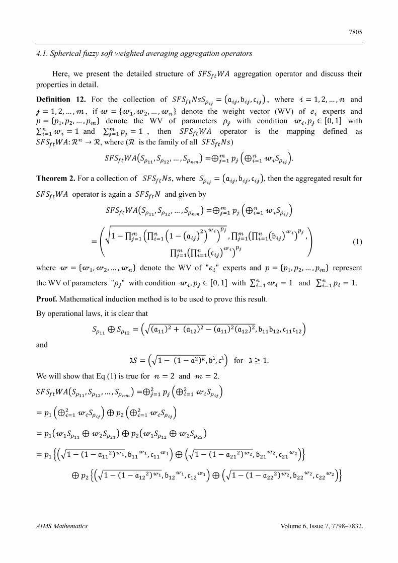
Definition 12. For the collection of 𝑆𝐹𝑆 𝑁𝑠𝑆𝒾𝒿
𝔞𝒾𝒿, 𝔟𝒾𝒿, 𝔠𝒾𝒿 , where 𝒾 1, 2, … , 𝓃 and
𝒿 1, 2, … , 𝓂 , if 𝓌 𝓌 , 𝓌 , … , 𝓌𝓃 denote the weight vector (WV) of ℯ𝒾 experts and 𝑝 𝑝 , 𝑝 , … , 𝑝𝓂 denote the WV of parameters 𝜌𝒿 with condition 𝓌𝒾, 𝑝𝒿 ∈ 0, 1 with ∑ 𝓌𝒾 1𝓃
𝒾 and ∑ 𝑝𝒿 1𝓂𝒿 , then 𝑆𝐹𝑆 𝑊𝐴 operator is the mapping defined as
𝑆𝐹𝑆 𝑊𝐴: ℛ𝓃 → ℛ, where (ℛ is the family of all 𝑆𝐹𝑆 𝑁𝑠)
𝑆𝐹𝑆 𝑊𝐴 𝑆 , 𝑆 , … , 𝑆𝓃𝓂
⊕𝒿𝓂 𝑝𝒿 ⊕𝒾
𝓃 𝓌𝒾𝑆𝒾𝒿
.
Theorem 2. For a collection of 𝑆𝐹𝑆 𝑁𝑠, where 𝑆𝒾𝒿
𝔞𝒾𝒿, 𝔟𝒾𝒿, 𝔠𝒾𝒿 , then the aggregated result for
𝑆𝐹𝑆 𝑊𝐴 operator is again a 𝑆𝐹𝑆 𝑁 and given by
𝑆𝐹𝑆 𝑊𝐴 𝑆 , 𝑆 , … , 𝑆𝓃𝓂
⊕𝒿𝓂 𝑝𝒿 ⊕𝒾
𝓃 𝓌𝒾𝑆𝒾𝒿
1 ∏ ∏ 1 𝔞𝒾𝒿
𝓌𝒾𝓃𝒾
𝒿𝓂𝒿 , ∏ ∏ 𝔟𝒾𝒿
𝓌𝒾𝓃𝒾
𝒿𝓂𝒿 ,
∏ ∏ 𝔠𝒾𝒿𝓌𝒾𝓃
𝒾𝒿𝓂
𝒿
(1)
where 𝓌 𝓌 , 𝓌 , … , 𝓌𝓃 denote the WV of "ℯ𝒾" experts and 𝑝 𝑝 , 𝑝 , … , 𝑝𝓂 represent
the WV of parameters "𝜌𝒿" with condition 𝓌𝒾, 𝑝𝒿 ∈ 0, 1 with ∑ 𝓌𝒾𝓃𝒾 1 and ∑ 𝑝𝒾 1𝓃
𝒾 .
Proof. Mathematical induction method is to be used to prove this result.
By operational laws, it is clear that
𝑆 ⊕ 𝑆 𝔞 𝔞 𝔞 𝔞 , 𝔟 𝔟 , 𝔠 𝔠
and
ℷ𝑆 1 1 𝔞 , 𝔟ℷ, 𝔠ℷ for ℷ 1.
We will show that Eq (1) is true for 𝓃 2 and 𝓂 2.
𝑆𝐹𝑆 𝑊𝐴 𝑆 , 𝑆 , … , 𝑆𝓃𝓂
⊕𝒿 𝑝𝒿 ⊕𝒾 𝓌𝒾𝑆𝒾𝒿
𝑝 ⊕𝒾 𝓌𝒾𝑆𝒾𝒿
⊕ 𝑝 ⊕𝒾 𝓌𝒾𝑆𝒾𝒿
𝑝 𝓌 𝑆 ⊕ 𝓌 𝑆 ⊕ 𝑝 𝓌 𝑆 ⊕ 𝓌 𝑆
𝑝 1 1 𝔞 𝓌 , 𝔟 𝓌 , 𝔠 𝓌 ⊕ 1 1 𝔞 𝓌 , 𝔟 𝓌 , 𝔠 𝓌
⊕ 𝑝 1 1 𝔞 𝓌 , 𝔟 𝓌 , 𝔠 𝓌 ⊕ 1 1 𝔞 𝓌 , 𝔟 𝓌 , 𝔠 𝓌
7806
AIMS Mathematics Volume 6, Issue 7, 7798–7832.
𝑝
⎝
⎛ 1 1 𝔞𝒾
𝒾
𝓌𝒾
, 𝔟𝒾𝓌𝒾
𝒾
, 𝔠𝒾𝓌𝒾
𝒾⎠
⎞
⊕ 𝜌
⎝
⎛ 1 1 𝔞𝒾
𝒾
𝓌𝒾
, 𝔟𝒾𝓌𝒾
𝒾
, 𝔠𝒾𝓌𝒾
𝒾⎠
⎞
⎝
⎛ 1 1 𝔞𝒾
𝒾
𝓌𝒾
, 𝔟𝒾𝓌𝒾
𝒾
, 𝔠𝒾𝓌𝒾
𝒾⎠
⎞
⊕
⎝
⎛ 1 1 𝔞𝒾
𝒾
𝓌𝒾
, 𝔟𝒾𝓌𝒾
𝒾
, 𝔠𝒾𝓌𝒾
𝒾⎠
⎞
1 ∏ ∏ 1 𝔞𝒾𝒿𝒾𝓌𝒾 𝒿
𝒿 , ∏ ∏ 𝔟𝒾𝒿𝓌𝒾
𝒾𝒿
𝒿 , ∏ ∏ 𝔠𝒾𝒿𝓌𝒾
𝒾𝒿
𝒿 .
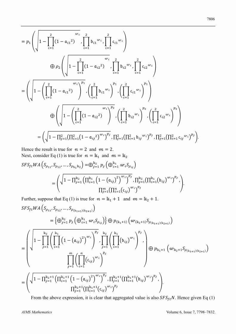
Hence the result is true for 𝓃 2 and 𝓂 2. Next, consider Eq (1) is true for 𝓃 𝕜 and 𝓂 𝕜
𝑆𝐹𝑆 𝑊𝐴 𝑆 , 𝑆 , … , 𝑆𝕜 𝕜 ⊕𝒿
𝕜 𝑝𝒿 ⊕𝒾𝕜 𝓌𝒾𝑆
𝒾𝒿
1 ∏ ∏ 1 𝔞𝒾𝒿
𝓌𝒾𝕜𝒾
𝒿𝕜𝒿 , ∏ ∏ 𝔟𝒾𝒿
𝓌𝒾𝕜𝒾
𝒿𝕜𝒿 ,
∏ ∏ 𝔠𝒾𝒿𝓌𝒾𝓃
𝒾𝒿𝓂
𝒿
.
Further, suppose that Eq (1) is true for 𝓃 𝕜 1 and 𝓂 𝕜 1.
𝑆𝐹𝑆 𝑊𝐴 𝑆 , 𝑆 , … , 𝑆𝕜 𝕜
⊕𝒿𝕜 𝑝𝒿 ⊕𝒾
𝕜 𝓌𝒾𝑆𝒾𝒿
⊕ 𝑝 𝕜 𝓌 𝕜 𝑆𝕜 𝕜
⎝
⎜⎜⎜⎛ 1 1 𝔞𝒾𝒿
𝓌𝒾
𝕜
𝒾
𝒿𝕜
𝒿
, 𝔟𝒾𝒿𝓌𝒾
𝕜
𝒾
𝒿𝕜
𝒿
,
𝔠𝒾𝒿𝓌𝒾
𝓃
𝒾
𝒿𝓂
𝒿 ⎠
⎟⎟⎟⎞
⊕ 𝑝𝕜 𝓌𝕜 𝑆𝕜 𝕜
1 ∏ ∏ 1 𝔞𝒾𝒿
𝓌𝒾𝕜𝒾
𝒿𝕜𝒿 , ∏ ∏ 𝔟𝒾𝒿
𝓌𝒾𝕜𝒾
𝒿𝕜𝒿 ,
∏ ∏ 𝔠𝒾𝒿𝓌𝒾𝕜
𝒾𝒿𝕜
𝒿
.
From the above expression, it is clear that aggregated value is also 𝑆𝐹𝑆 𝑁. Hence given Eq (1)
7807
AIMS Mathematics Volume 6, Issue 7, 7798–7832.
is true for 𝓃 𝕜 1 and 𝓂 𝕜 1. Hence it is true for all 𝓂, 𝓃 1.
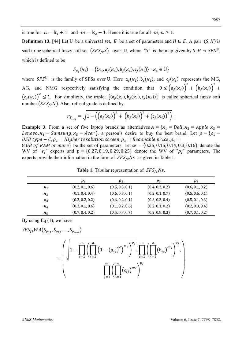
Definition 13. [44] Let 𝕌 be a universal set, 𝐸 be a set of parameters and 𝛨 ⊆ 𝐸. A pair 𝑆, 𝛨 is
said to be spherical fuzzy soft set 𝑆𝐹𝑆 𝑆 over 𝕌, where "𝑆" is the map given by 𝑆: 𝛨 → 𝑆𝐹𝑆𝕌,
which is defined to be
𝑆𝒿
𝜘𝒾 ⟨𝜘𝒾, 𝔞𝒿 𝜘𝒾 , 𝔟𝒿 𝜘𝒾 , 𝔠𝒿 𝜘𝒾 ⟩ ∶ 𝜘𝒾 ∈ 𝕌
where 𝑆𝐹𝑆𝕌 is the family of SFSs over 𝕌. Here 𝔞𝒿 𝜘𝒾 , 𝔟𝒿 𝜘𝒾 , and 𝔠𝒿 𝜘𝒾 represents the MG,
AG, and NMG respectively satisfying the condition that 0 𝔞𝒿 𝜘𝒾 𝔟𝒿 𝜘𝒾
𝔠𝒿 𝜘𝒾 1. For simplicity, the triplet ⟨𝔞𝒿 𝜘𝒾 , 𝔟𝒿 𝜘𝒾 , 𝔠𝒿 𝜘𝒾 ⟩ is called spherical fuzzy soft
number 𝑆𝐹𝑆 𝑁 . Also, refusal grade is defined by
𝓇𝒾𝒿
1 𝔞𝒿 𝜘𝒾 𝔟𝒿 𝜘𝒾 𝔠𝒿 𝜘𝒾 .
Example 3. From a set of five laptop brands as alternatives 𝐴 𝜘 𝐷𝑒𝑙𝑙, 𝜘 𝐴𝑝𝑝𝑙𝑒, 𝜘𝐿𝑒𝑛𝑜𝑣𝑜, 𝜘 𝑆𝑎𝑚𝑠𝑢𝑛𝑔, 𝜘 𝐴𝑐𝑒𝑟 , a person’s desire to buy the best brand. Let 𝜌 𝜌𝑈𝑆𝐵 𝑡𝑦𝑝𝑒 𝐶, 𝜌 𝐻𝑖𝑔ℎ𝑒𝑟 𝑟𝑒𝑠𝑜𝑙𝑢𝑡𝑖𝑜𝑛 𝑠𝑐𝑟𝑒𝑒𝑛, 𝜌 𝑅𝑒𝑎𝑜𝑛𝑎𝑏𝑙𝑒 𝑝𝑟𝒾𝑐ℯ, 𝜌8 𝐺𝐵 𝑜𝑓 𝑅𝐴𝑀 𝑜𝑟 𝑚𝑜𝑟𝑒 be the set of parameters. Let 𝓌 0.25, 0.15, 0.14, 0.3, 0,16 denote the WV of "ℯ𝒾" experts and 𝑝 0.27, 0.19, 0.29, 0.25 denote the WV of "𝜌𝒿" parameters. The experts provide their information in the form of 𝑆𝐹𝑆 𝑁𝑠 as given in Table 1.
Table 1. Tabular representation of 𝑆𝐹𝑆 𝑁𝑠.
𝝆𝟏 𝝆𝟐 𝝆𝟑 𝝆𝟒
𝝒𝟏 0.2, 0.1, 0.6 0.5, 0.3, 0.1 0.4, 0.3, 0.2 0.6, 0.1, 0.2
𝝒𝟐 0.1, 0.4, 0.4 0.6, 0.3, 0.1 0.2, 0.1, 0.7 0.5, 0.6, 0.1
𝝒𝟑 0.3, 0.2, 0.2 0.6, 0.2, 0.1 0.3, 0.3, 0.4 0.5, 0.1, 0.3
𝝒𝟒 0.3, 0.1, 0.6 0.1, 0.2, 0.6 0.2, 0.1, 0.2 0.2, 0.3, 0.4
𝝒𝟓 0.7, 0.4, 0.2 0.5, 0.3, 0.7 0.2, 0.8, 0.3 0.7, 0.1, 0.2
By using Eq (1), we have
𝑆𝐹𝑆 𝑊𝐴 𝑆 , 𝑆 , … , 𝑆𝓃𝓂
⎝
⎜⎜⎜⎛ 1 1 𝔞𝒾𝒿
𝓌𝒾𝓃
𝒾
𝒿𝓂
𝒿
, 𝔟𝒾𝒿𝓌𝒾
𝓃
𝒾
𝒿𝓂
𝒿
,
𝔠𝒾𝒿𝓌𝒾
𝓃
𝒾
𝒿𝓂
𝒿 ⎠
⎟⎟⎟⎞
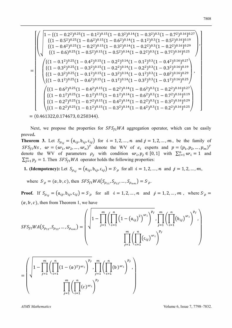
7808
AIMS Mathematics Volume 6, Issue 7, 7798–7832.
⎣⎢⎢⎢⎢⎢⎢⎢⎢⎢⎢⎢⎢⎢⎢⎡
⎝
⎜⎛
1 1 0.2 . 1 0.1 . 1 0.3 . 1 0.3 . 1 0.7 . .
1 0.5 . 1 0.6 . 1 0.6 . 1 0.1 . 1 0.5 . .
1 0.4 . 1 0.2 . 1 0.3 . 1 0.2 . 1 0.2 . .
1 0.6 . 1 0.5 . 1 0.5 . 1 0.2 . 1 0.7 . .⎠
⎟⎞
,
⎝
⎜⎛
1 0.1 . 1 0.4 . 1 0.2 . 1 0.1 . 1 0.4 . .
1 0.3 . 1 0.3 . 1 0.2 . 1 0.2 . 1 0.3 . .
1 0.3 . 1 0.1 . 1 0.3 . 1 0.1 . 1 0.8 . .
1 0.1 . 1 0.6 . 1 0.1 . 1 0.3 . 1 0.1 . .⎠
⎟⎞
,
⎝
⎜⎛
1 0.6 . 1 0.4 . 1 0.2 . 1 0.6 . 1 0.2 . .
1 0.1 . 1 0.1 . 1 0.1 . 1 0.6 . 1 0.7 . .
1 0.2 . 1 0.7 . 1 0.4 . 1 0.2 . 1 0.3 . .
1 0.2 . 1 0.1 . 1 0.3 . 1 0.4 . 1 0.2 . .⎠
⎟⎞
⎦⎥⎥⎥⎥⎥⎥⎥⎥⎥⎥⎥⎥⎥⎥⎤
0.461322,0.174673, 0.250344 .
Next, we propose the properties for 𝑆𝐹𝑆 𝑊𝐴 aggregation operator, which can be easily proved. Theorem 3. Let 𝑆
𝒾𝒿𝔞𝒾𝒿, 𝔟𝒾𝒿, 𝔠𝒾𝒿 for 𝒾 1, 2, … , 𝓃 and 𝒿 1, 2, … , 𝓂 , be the family of
𝑆𝐹𝑆 𝑁𝑠 , 𝓌 𝓌 , 𝓌 , … , 𝓌𝓃 denote the WV of ℯ𝒾 experts and 𝑝 𝑝 , 𝑝 , … , 𝑝𝓂 denote the WV of parameters 𝜌𝒿 with condition 𝓌𝒾, 𝑝𝒿 ∈ 0, 1 with ∑ 𝓌𝒾 1𝓃
𝒾 and ∑ 𝑝𝒿 1𝓂
𝒿 . Then 𝑆𝐹𝑆 𝑊𝐴 operator holds the following properties:
1. (Idempotency): Let 𝑆𝒾𝒿
𝔞𝒾𝒿, 𝔟𝒾𝒿, 𝔠𝒾𝒿 𝑆, for all 𝒾 1, 2, … , 𝓃 and 𝒿 1, 2, … , 𝓂,
where 𝑆, 𝔞,, 𝔟,, 𝔠, , then 𝑆𝐹𝑆 𝑊𝐴 𝑆 , 𝑆 , … , 𝑆𝓃𝓂
𝑆, .
Proof. If 𝑆𝒾𝒿
𝔞𝒾𝒿, 𝔟𝒾𝒿, 𝔠𝒾𝒿 𝑆, for all 𝒾 1, 2, … , 𝓃 and 𝒿 1, 2, … , 𝓂 , where 𝑆,
𝔞,, 𝔟,, 𝔠, , then from Theorem 1, we have
𝑆𝐹𝑆 𝑊𝐴 𝑆 , 𝑆 , … , 𝑆𝓃𝓂
⎝
⎜⎜⎜⎛ 1 1 𝔞𝒾𝒿
𝓌𝒾𝓃
𝒾
𝒿𝓂
𝒿
, 𝔟𝒾𝒿𝓌𝒾
𝓃
𝒾
𝒿𝓂
𝒿
,
𝔠𝒾𝒿𝓌𝒾
𝓃
𝒾
𝒿𝓂
𝒿 ⎠
⎟⎟⎟⎞
⎝
⎜⎜⎜⎛ 1 1 𝔞, 𝓌𝒾
𝓃
𝒾
𝒿𝓂
𝒿
, 𝔟, 𝓌𝒾
𝓃
𝒾
𝒿𝓂
𝒿
,
𝔠, 𝓌𝒾
𝓃
𝒾
𝒿𝓂
𝒿 ⎠
⎟⎟⎟⎞
7809
AIMS Mathematics Volume 6, Issue 7, 7798–7832.
1 1 𝔞, , 𝔟,, 𝔠, 𝔞,, 𝔟,, 𝔠, 𝑆, .
Hence 𝑆𝐹𝑆 𝑊𝐴 𝑆 , 𝑆 , … , 𝑆𝓃𝓂
𝑆, .
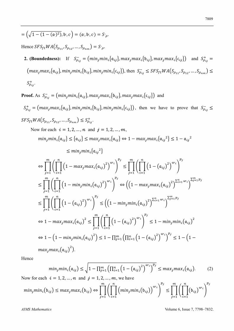
2. (Boundedness): If 𝑆𝒾𝒿
𝑚𝑖𝑛𝒿𝑚𝑖𝑛𝒾 𝔞𝒾𝒿 , 𝑚𝑎𝑥𝒿𝑚𝑎𝑥𝒾 𝔟𝒾𝒿 , 𝑚𝑎𝑥𝒿𝑚𝑎𝑥𝒾 𝔠𝒾𝒿 and 𝑆𝒾𝒿
𝑚𝑎𝑥𝒿𝑚𝑎𝑥𝒾 𝔞𝒾𝒿 , 𝑚𝑖𝑛𝒿𝑚𝑖𝑛𝒾 𝔟𝒾𝒿 , 𝑚𝑖𝑛𝒿𝑚𝑖𝑛𝒾 𝔠𝒾𝒿 , then 𝑆𝒾𝒿
𝑆𝐹𝑆 𝑊𝐴 𝑆 , 𝑆 , … , 𝑆𝓃𝓂
𝑆𝒾𝒿
.
Proof. As 𝑆𝒾𝒿
𝑚𝑖𝑛𝒿𝑚𝑖𝑛𝒾 𝔞𝒾𝒿 , 𝑚𝑎𝑥𝒿𝑚𝑎𝑥𝒾 𝔟𝒾𝒿 , 𝑚𝑎𝑥𝒿𝑚𝑎𝑥𝒾 𝔠𝒾𝒿 and
𝑆𝒾𝒿
𝑚𝑎𝑥𝒿𝑚𝑎𝑥𝒾 𝔞𝒾𝒿 , 𝑚𝑖𝑛𝒿𝑚𝑖𝑛𝒾 𝔟𝒾𝒿 , 𝑚𝑖𝑛𝒿𝑚𝑖𝑛𝒾 𝔠𝒾𝒿 , then we have to prove that 𝑆𝒾𝒿
𝑆𝐹𝑆 𝑊𝐴 𝑆 , 𝑆 , … , 𝑆𝓃𝓂
𝑆𝒾𝒿
.
Now for each 𝒾 1, 2, … , 𝓃 and 𝒿 1, 2, … , 𝓂,
𝑚𝑖𝑛𝒿𝑚𝑖𝑛𝒾 𝔞𝒾𝒿 𝔞𝒾𝒿 𝑚𝑎𝑥𝒿𝑚𝑎𝑥𝒾 𝔞𝒾𝒿 ⇔ 1 𝑚𝑎𝑥𝒿𝑚𝑎𝑥𝒾 𝔞𝒾𝒿 1 𝔞𝒾𝒿
𝑚𝑖𝑛𝒿𝑚𝑖𝑛𝒾 𝔞𝒾𝒿
⇔ 1 𝑚𝑎𝑥𝒿𝑚𝑎𝑥𝒾 𝔞𝒾𝒿
𝓌𝒾𝓃
𝒾
𝒿𝓂
𝒿
1 𝔞𝒾𝒿
𝓌𝒾𝓃
𝒾
𝒿𝓂
𝒿
1 𝑚𝑖𝑛𝒿𝑚𝑖𝑛𝒾 𝔞𝒾𝒿
𝓌𝒾𝓃
𝒾
𝒿
⇔ 1 𝑚𝑎𝑥𝒿𝑚𝑎𝑥𝒾 𝔞𝒾𝒿
∑ 𝓌𝒾𝓃𝒾
∑ 𝒿𝓂𝒿
𝓂
𝒿
1 𝔞𝒾𝒿
𝓌𝒾𝓃
𝒾
𝒿𝓂
𝒿
1 𝑚𝑖𝑛𝒿𝑚𝑖𝑛𝒾 𝔞𝒾𝒿
∑ 𝓌𝒾𝓃𝒾
∑ 𝒿𝓂𝒿
⇔ 1 𝑚𝑎𝑥𝒿𝑚𝑎𝑥𝒾 𝔞𝒾𝒿 1 𝔞𝒾𝒿
𝓌𝒾𝓃
𝒾
𝒿𝓂
𝒿
1 𝑚𝑖𝑛𝒿𝑚𝑖𝑛𝒾 𝔞𝒾𝒿
⇔ 1 1 𝑚𝑖𝑛𝒿𝑚𝑖𝑛𝒾 𝔞𝒾𝒿 1 ∏ ∏ 1 𝔞𝒾𝒿
𝓌𝒾𝓃𝒾
𝒿𝓂𝒿 1 1
𝑚𝑎𝑥𝒿𝑚𝑎𝑥𝒾 𝔞𝒾𝒿 .
Hence
𝑚𝑖𝑛𝒿𝑚𝑖𝑛𝒾 𝔞𝒾𝒿 1 ∏ ∏ 1 𝔞𝒾𝒿
𝓌𝒾𝓃𝒾
𝒿𝓂𝒿 𝑚𝑎𝑥𝒿𝑚𝑎𝑥𝒾 𝔞𝒾𝒿 . (2)
Now for each 𝒾 1, 2, … , 𝓃 and 𝒿 1, 2, … , 𝓂, we have
𝑚𝑖𝑛𝒿𝑚𝑖𝑛𝒾 𝔟𝒾𝒿 𝑚𝑎𝑥𝒿𝑚𝑎𝑥𝒾 𝔟𝒾𝒿 ⇔ 𝑚𝑖𝑛𝒿𝑚𝑖𝑛𝒾 𝔟𝒾𝒿
𝓌𝒾𝓃
𝒾
𝒿𝓂
𝒿
𝔟𝒾𝒿𝓌𝒾
𝓃
𝒾
𝒿𝓂
𝒿
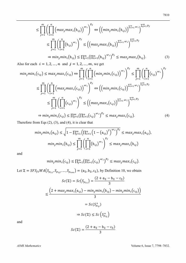
7810
AIMS Mathematics Volume 6, Issue 7, 7798–7832.
𝑚𝑎𝑥𝒿𝑚𝑎𝑥𝒾 𝔟𝒾𝒿
𝓌𝒾𝓃
𝒾
𝒿𝓂
𝒿
⇔ 𝑚𝑖𝑛𝒿𝑚𝑖𝑛𝒾 𝔟𝒾𝒿
∑ 𝓌𝒾𝓃𝒾
∑ 𝒿𝓂𝒿
𝔟𝒾𝒿𝓌𝒾
𝓃
𝒾
𝒿𝓂
𝒿
𝑚𝑎𝑥𝒿𝑚𝑎𝑥𝒾 𝔟𝒾𝒿
∑ 𝓌𝒾𝓃𝒾
∑ 𝒿𝓂𝒿
⇒ 𝑚𝑖𝑛𝒿𝑚𝑖𝑛𝒾 𝔟𝒾𝒿 ∏ ∏ 𝔟𝒾𝒿𝓌𝒾𝓃
𝒾𝒿𝓂
𝒿 𝑚𝑎𝑥𝒿𝑚𝑎𝑥𝒾 𝔟𝒾𝒿 . (3)
Also for each 𝒾 1, 2, … , 𝓃 and 𝒿 1, 2, … , 𝓂, we get
𝑚𝑖𝑛𝒿𝑚𝑖𝑛𝒾 𝔠𝒾𝒿 𝑚𝑎𝑥𝒿𝑚𝑎𝑥𝒾 𝔠𝒾𝒿 ⇔ 𝑚𝑖𝑛𝒿𝑚𝑖𝑛𝒾 𝔠𝒾𝒿
𝓌𝒾𝓃
𝒾
𝒿𝓂
𝒿
𝔠𝒾𝒿𝓌𝒾
𝓃
𝒾
𝒿𝓂
𝒿
𝑚𝑎𝑥𝒿𝑚𝑎𝑥𝒾 𝔠𝒾𝒿
𝓌𝒾𝓃
𝒾
𝒿𝓂
𝒿
⇔ 𝑚𝑖𝑛𝒿𝑚𝑖𝑛𝒾 𝔠𝒾𝒿
∑ 𝓌𝒾𝓃𝒾
∑ 𝒿𝓂𝒿
𝔠𝒾𝒿𝓌𝒾
𝓃
𝒾
𝒿𝓂
𝒿
𝑚𝑎𝑥𝒿𝑚𝑎𝑥𝒾 𝔠𝒾𝒿
∑ 𝓌𝒾𝓃𝒾
∑ 𝒿𝓂𝒿
⇒ 𝑚𝑖𝑛𝒿𝑚𝑖𝑛𝒾 𝔠𝒾𝒿 ∏ ∏ 𝔠𝒾𝒿𝓌𝒾𝓃
𝒾𝒿𝓂
𝒿 𝑚𝑎𝑥𝒿𝑚𝑎𝑥𝒾 𝔠𝒾𝒿 . (4)
Therefore from Eqs (2), (3), and (4), it is clear that
𝑚𝑖𝑛𝒿𝑚𝑖𝑛𝒾 𝔞𝒾𝒿 1 ∏ ∏ 1 𝔞𝒾𝒿
𝓌𝒾𝓃𝒾
𝒿𝓂𝒿 𝑚𝑎𝑥𝒿𝑚𝑎𝑥𝒾 𝔞𝒾𝒿 ,
𝑚𝑖𝑛𝒿𝑚𝑖𝑛𝒾 𝔟𝒾𝒿 𝔟𝒾𝒿𝓌𝒾
𝓃
𝒾
𝒿𝓂
𝒿
𝑚𝑎𝑥𝒿𝑚𝑎𝑥𝒾 𝔟𝒾𝒿
and
𝑚𝑖𝑛𝒿𝑚𝑖𝑛𝒾 𝔠𝒾𝒿 ∏ ∏ 𝔠𝒾𝒿𝓌𝒾𝓃
𝒾𝒿𝓂
𝒿 𝑚𝑎𝑥𝒿𝑚𝑎𝑥𝒾 𝔠𝒾𝒿 .
Let 𝔗 𝑆𝐹𝑆 𝑊𝐴 𝑆 , 𝑆 , … , 𝑆𝓃𝓂
𝔞𝔗, 𝔟𝔗, 𝔠𝔗 , by Definition 10, we obtain
𝑆𝑐 𝔗 𝑆𝑐 𝑆2 𝔞𝔗 𝔟𝔗 𝔠𝔗
3
2 𝑚𝑎𝑥𝒿𝑚𝑎𝑥𝒾 𝔞𝒾𝒿 𝑚𝑖𝑛𝒿𝑚𝑖𝑛𝒾 𝔟𝒾𝒿 𝑚𝑖𝑛𝒿𝑚𝑖𝑛𝒾 𝔠𝒾𝒿
3
𝑆𝑐 𝑆𝒾𝒿
⇒ 𝑆𝑐 𝔗 𝑆𝑐 𝑆𝒾𝒿
and
𝑆𝑐 𝔗2 𝔞𝔗 𝔟𝔗 𝔠𝔗
3
7811
AIMS Mathematics Volume 6, Issue 7, 7798–7832.
2 𝑚𝑖𝑛𝒿𝑚𝑖𝑛𝒾 𝔞𝒾𝒿 𝑚𝑎𝑥𝒿𝑚𝑎𝑥𝒾 𝔟𝒾𝒿 𝑚𝑎𝑥𝒿𝑚𝑎𝑥𝒾 𝔠𝒾𝒿
3
𝑆𝑐 𝑆𝒾𝒿
⇒ 𝑆𝑐 𝔗 𝑆𝑐 𝑆𝒾𝒿
.
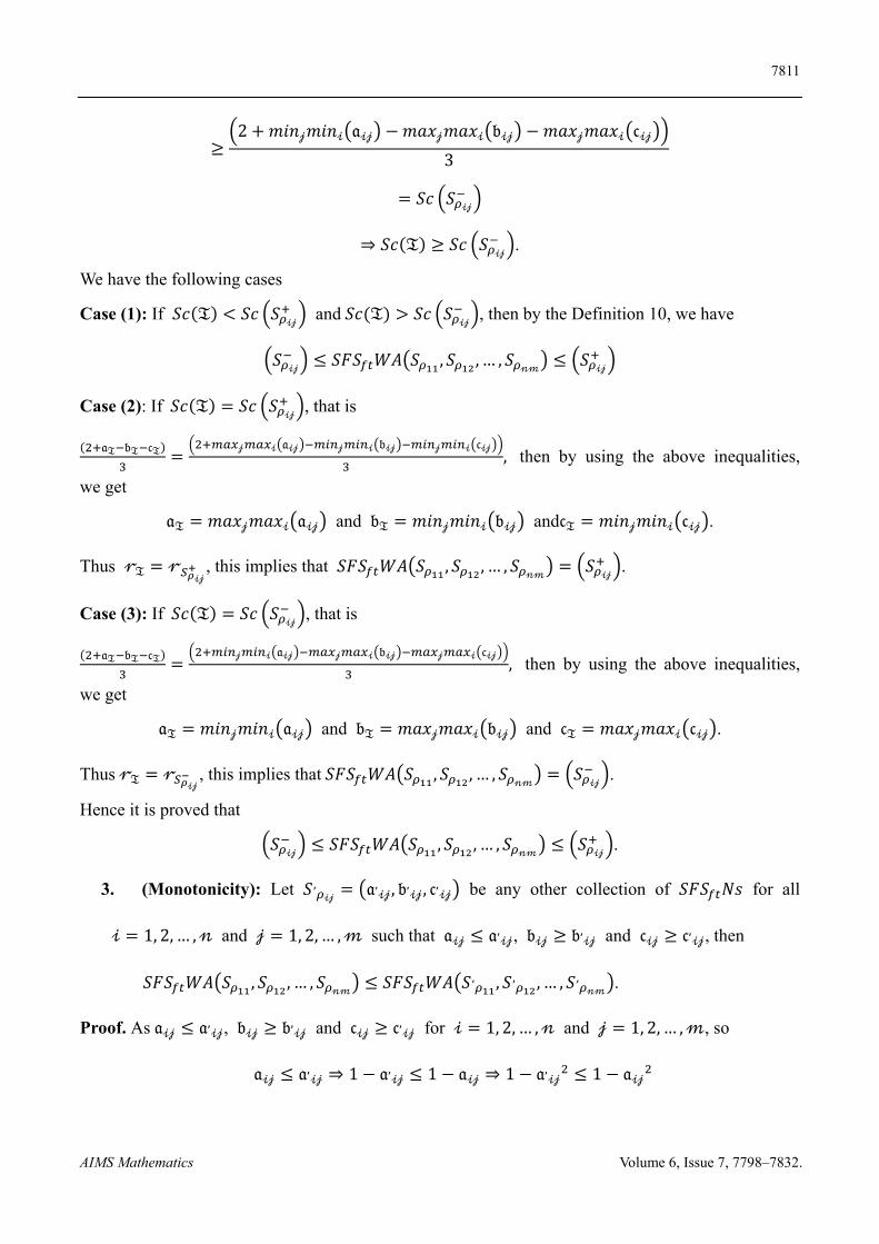
We have the following cases
Case (1): If 𝑆𝑐 𝔗 𝑆𝑐 𝑆𝒾𝒿
and 𝑆𝑐 𝔗 𝑆𝑐 𝑆𝒾𝒿
, then by the Definition 10, we have
𝑆𝒾𝒿
𝑆𝐹𝑆 𝑊𝐴 𝑆 , 𝑆 , … , 𝑆𝓃𝓂
𝑆𝒾𝒿
Case (2): If 𝑆𝑐 𝔗 𝑆𝑐 𝑆𝒾𝒿
, that is
𝔞𝔗 𝔟𝔗 𝔠𝔗 𝒿 𝒾 𝔞𝒾𝒿 𝒿 𝒾 𝔟𝒾𝒿 𝒿 𝒾 𝔠𝒾𝒿, then by using the above inequalities,
we get
𝔞𝔗 𝑚𝑎𝑥𝒿𝑚𝑎𝑥𝒾 𝔞𝒾𝒿 and 𝔟𝔗 𝑚𝑖𝑛𝒿𝑚𝑖𝑛𝒾 𝔟𝒾𝒿 and𝔠𝔗 𝑚𝑖𝑛𝒿𝑚𝑖𝑛𝒾 𝔠𝒾𝒿 .
Thus 𝓇𝔗 𝓇𝒾𝒿
, this implies that 𝑆𝐹𝑆 𝑊𝐴 𝑆 , 𝑆 , … , 𝑆𝓃𝓂
𝑆𝒾𝒿
.
Case (3): If 𝑆𝑐 𝔗 𝑆𝑐 𝑆𝒾𝒿
, that is
𝔞𝔗 𝔟𝔗 𝔠𝔗 𝒿 𝒾 𝔞𝒾𝒿 𝒿 𝒾 𝔟𝒾𝒿 𝒿 𝒾 𝔠𝒾𝒿, then by using the above inequalities,
we get
𝔞𝔗 𝑚𝑖𝑛𝒿𝑚𝑖𝑛𝒾 𝔞𝒾𝒿 and 𝔟𝔗 𝑚𝑎𝑥𝒿𝑚𝑎𝑥𝒾 𝔟𝒾𝒿 and 𝔠𝔗 𝑚𝑎𝑥𝒿𝑚𝑎𝑥𝒾 𝔠𝒾𝒿 .
Thus 𝓇𝔗 𝓇𝒾𝒿
, this implies that 𝑆𝐹𝑆 𝑊𝐴 𝑆 , 𝑆 , … , 𝑆𝓃𝓂
𝑆𝒾𝒿
.
Hence it is proved that
𝑆𝒾𝒿
𝑆𝐹𝑆 𝑊𝐴 𝑆 , 𝑆 , … , 𝑆𝓃𝓂
𝑆𝒾𝒿
.
3. (Monotonicity): Let 𝑆,𝒾𝒿
𝔞,𝒾𝒿, 𝔟,
𝒾𝒿, 𝔠,𝒾𝒿 be any other collection of 𝑆𝐹𝑆 𝑁𝑠 for all
𝒾 1, 2, … , 𝓃 and 𝒿 1, 2, … , 𝓂 such that 𝔞𝒾𝒿 𝔞,𝒾𝒿, 𝔟𝒾𝒿 𝔟,
𝒾𝒿 and 𝔠𝒾𝒿 𝔠,𝒾𝒿, then
𝑆𝐹𝑆 𝑊𝐴 𝑆 , 𝑆 , … , 𝑆𝓃𝓂
𝑆𝐹𝑆 𝑊𝐴 𝑆, , 𝑆, , … , 𝑆,𝓃𝓂
.
Proof. As 𝔞𝒾𝒿 𝔞,𝒾𝒿, 𝔟𝒾𝒿 𝔟,
𝒾𝒿 and 𝔠𝒾𝒿 𝔠,𝒾𝒿 for 𝒾 1, 2, … , 𝓃 and 𝒿 1, 2, … , 𝓂, so
𝔞𝒾𝒿 𝔞,𝒾𝒿 ⇒ 1 𝔞,
𝒾𝒿 1 𝔞𝒾𝒿 ⇒ 1 𝔞,𝒾𝒿 1 𝔞𝒾𝒿
7812
AIMS Mathematics Volume 6, Issue 7, 7798–7832.
⇒ 1 𝔞,𝒾𝒿
𝓌𝒾𝓃
𝒾
𝒿𝓂
𝒿
1 𝔞𝒾𝒿
𝓌𝒾𝓃
𝒾
𝒿𝓂
𝒿
⇒ 1 1 𝔞𝒾𝒿
𝓌𝒾𝓃
𝒾
𝒿
1
𝓂
𝒿
1 𝔞,𝒾𝒿
𝓌𝒾𝓃
𝒾
𝒿𝓂
𝒿
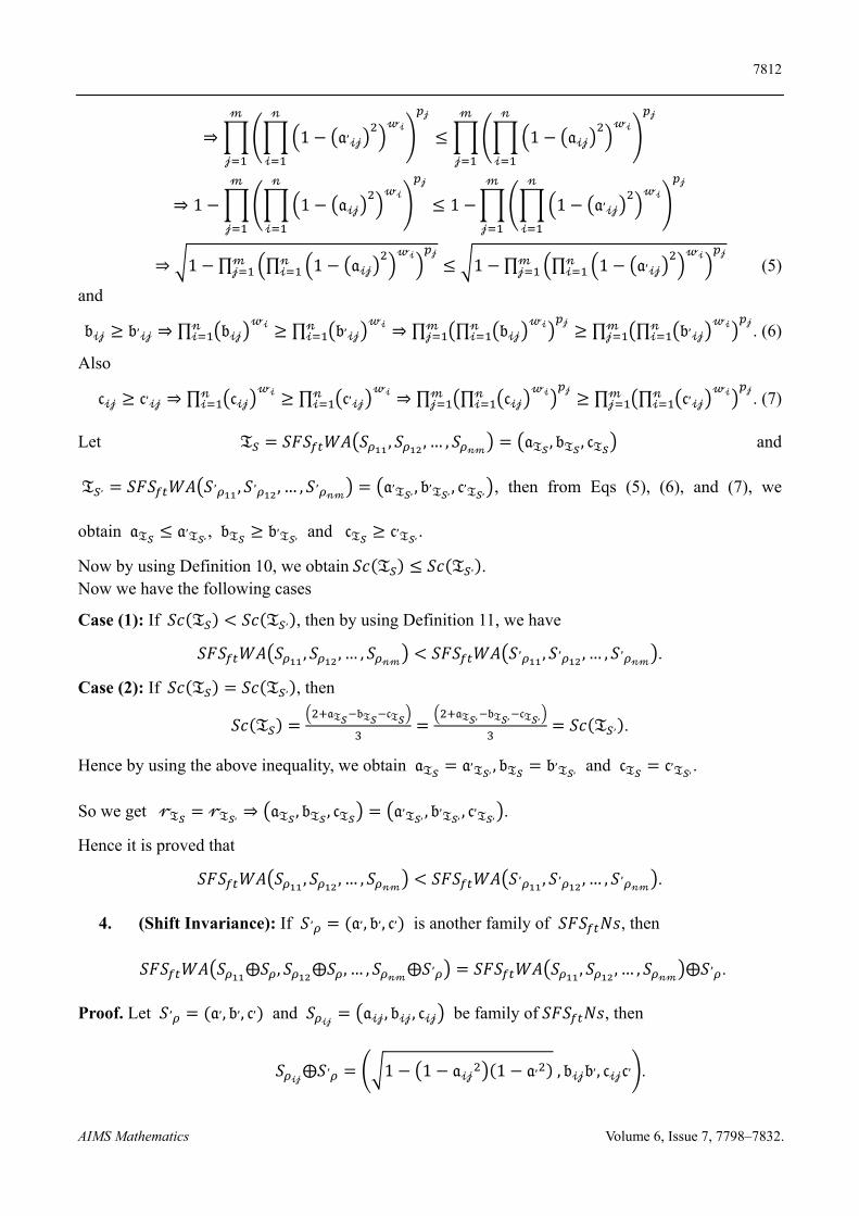
⇒ 1 ∏ ∏ 1 𝔞𝒾𝒿
𝓌𝒾𝓃𝒾
𝒿𝓂𝒿 1 ∏ ∏ 1 𝔞,
𝒾𝒿
𝓌𝒾𝓃𝒾
𝒿𝓂𝒿 (5)
and
𝔟𝒾𝒿 𝔟,𝒾𝒿 ⇒ ∏ 𝔟𝒾𝒿
𝓌𝒾𝓃𝒾 ∏ 𝔟,
𝒾𝒿𝓌𝒾𝓃
𝒾 ⇒ ∏ ∏ 𝔟𝒾𝒿𝓌𝒾𝓃
𝒾𝒿𝓂
𝒿 ∏ ∏ 𝔟,𝒾𝒿
𝓌𝒾𝓃𝒾
𝒿𝓂𝒿 . (6)
Also
𝔠𝒾𝒿 𝔠,𝒾𝒿 ⇒ ∏ 𝔠𝒾𝒿
𝓌𝒾𝓃𝒾 ∏ 𝔠,
𝒾𝒿𝓌𝒾𝓃
𝒾 ⇒ ∏ ∏ 𝔠𝒾𝒿𝓌𝒾𝓃
𝒾𝒿𝓂
𝒿 ∏ ∏ 𝔠,𝒾𝒿
𝓌𝒾𝓃𝒾
𝒿𝓂𝒿 . (7)
Let 𝔗 𝑆𝐹𝑆 𝑊𝐴 𝑆 , 𝑆 , … , 𝑆𝓃𝓂
𝔞𝔗 , 𝔟𝔗 , 𝔠𝔗 and
𝔗 , 𝑆𝐹𝑆 𝑊𝐴 𝑆, , 𝑆, , … , 𝑆,𝓃𝓂
𝔞,𝔗 , , 𝔟,
𝔗 , , 𝔠,𝔗 , , then from Eqs (5), (6), and (7), we
obtain 𝔞𝔗 𝔞,𝔗 , , 𝔟𝔗 𝔟,
𝔗 , and 𝔠𝔗 𝔠,𝔗 , .
Now by using Definition 10, we obtain 𝑆𝑐 𝔗 𝑆𝑐 𝔗 , . Now we have the following cases
Case (1): If 𝑆𝑐 𝔗 𝑆𝑐 𝔗 , , then by using Definition 11, we have
𝑆𝐹𝑆 𝑊𝐴 𝑆 , 𝑆 , … , 𝑆𝓃𝓂
𝑆𝐹𝑆 𝑊𝐴 𝑆, , 𝑆, , … , 𝑆,𝓃𝓂
.
Case (2): If 𝑆𝑐 𝔗 𝑆𝑐 𝔗 , , then
𝑆𝑐 𝔗𝔞𝔗 𝔟𝔗 𝔠𝔗 𝔞𝔗 , 𝔟𝔗 , 𝔠𝔗 ,
𝑆𝑐 𝔗 , .
Hence by using the above inequality, we obtain 𝔞𝔗 𝔞,𝔗 , , 𝔟𝔗 𝔟,
𝔗 , and 𝔠𝔗 𝔠,𝔗 , .
So we get 𝓇𝔗 𝓇𝔗 , ⇒ 𝔞𝔗 , 𝔟𝔗 , 𝔠𝔗 𝔞,𝔗 , , 𝔟,
𝔗 , , 𝔠,𝔗 , .
Hence it is proved that
𝑆𝐹𝑆 𝑊𝐴 𝑆 , 𝑆 , … , 𝑆𝓃𝓂
𝑆𝐹𝑆 𝑊𝐴 𝑆, , 𝑆, , … , 𝑆,𝓃𝓂
.
4. (Shift Invariance): If 𝑆, 𝔞,, 𝔟,, 𝔠, is another family of 𝑆𝐹𝑆 𝑁𝑠, then
𝑆𝐹𝑆 𝑊𝐴 𝑆 ⨁𝑆 , 𝑆 ⨁𝑆 , … , 𝑆𝓃𝓂
⨁𝑆, 𝑆𝐹𝑆 𝑊𝐴 𝑆 , 𝑆 , … , 𝑆𝓃𝓂
⨁𝑆, .
Proof. Let 𝑆, 𝔞,, 𝔟,, 𝔠, and 𝑆𝒾𝒿
𝔞𝒾𝒿, 𝔟𝒾𝒿, 𝔠𝒾𝒿 be family of 𝑆𝐹𝑆 𝑁𝑠, then
𝑆𝒾𝒿
⨁𝑆, 1 1 𝔞𝒾𝒿 1 𝔞, , 𝔟𝒾𝒿𝔟,, 𝔠𝒾𝒿𝔠, .
7813
AIMS Mathematics Volume 6, Issue 7, 7798–7832.
Therefore,
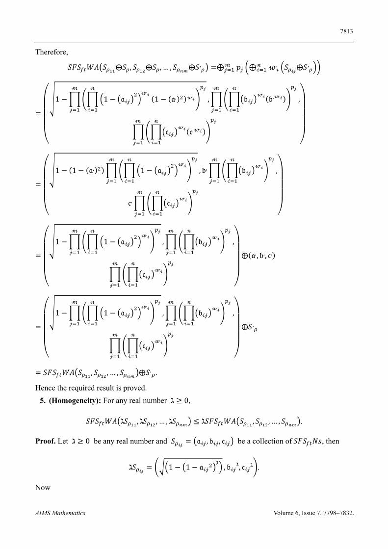
𝑆𝐹𝑆 𝑊𝐴 𝑆 ⨁𝑆 , 𝑆 ⨁𝑆 , … , 𝑆𝓃𝓂
⨁𝑆, ⊕𝒿𝓂 𝑝𝒿 ⊕𝒾
𝓃 𝓌𝒾 𝑆𝒾𝒿
⨁𝑆,
⎝
⎜⎜⎜⎛ 1 1 𝔞𝒾𝒿
𝓌𝒾𝓃
𝒾
1 𝔞, 𝓌𝒾
𝒿𝓂
𝒿
, 𝔟𝒾𝒿𝓌𝒾 𝔟,𝓌𝒾
𝓃
𝒾
𝒿𝓂
𝒿
,
𝔠𝒾𝒿𝓌𝒾 𝔠,𝓌𝒾
𝓃
𝒾
𝒿𝓂
𝒿 ⎠
⎟⎟⎟⎞
⎝
⎜⎜⎜⎛ 1 1 𝔞, 1 𝔞𝒾𝒿
𝓌𝒾𝓃
𝒾
𝒿𝓂
𝒿
, 𝔟, 𝔟𝒾𝒿𝓌𝒾
𝓃
𝒾
𝒿𝓂
𝒿
,
𝔠, 𝔠𝒾𝒿𝓌𝒾
𝓃
𝒾
𝒿𝓂
𝒿 ⎠
⎟⎟⎟⎞
⎝
⎜⎜⎜⎛ 1 1 𝔞𝒾𝒿
𝓌𝒾𝓃
𝒾
𝒿𝓂
𝒿
, 𝔟𝒾𝒿𝓌𝒾
𝓃
𝒾
𝒿𝓂
𝒿
,
𝔠𝒾𝒿𝓌𝒾
𝓃
𝒾
𝒿𝓂
𝒿 ⎠
⎟⎟⎟⎞
⨁ 𝔞,, 𝔟,, 𝔠,
⎝
⎜⎜⎜⎛ 1 1 𝔞𝒾𝒿
𝓌𝒾𝓃
𝒾
𝒿𝓂
𝒿
, 𝔟𝒾𝒿𝓌𝒾
𝓃
𝒾
𝒿𝓂
𝒿
,
𝔠𝒾𝒿𝓌𝒾
𝓃
𝒾
𝒿𝓂
𝒿 ⎠
⎟⎟⎟⎞
⨁𝑆,
𝑆𝐹𝑆 𝑊𝐴 𝑆 , 𝑆 , … , 𝑆𝓃𝓂
⨁𝑆, .
Hence the required result is proved.
5. (Homogeneity): For any real number ℷ 0,
𝑆𝐹𝑆 𝑊𝐴 ℷ𝑆 , ℷ𝑆 , … , ℷ𝑆𝓃𝓂
ℷ𝑆𝐹𝑆 𝑊𝐴 𝑆 , 𝑆 , … , 𝑆𝓃𝓂
.
Proof. Let ℷ 0 be any real number and 𝑆𝒾𝒿
𝔞𝒾𝒿, 𝔟𝒾𝒿, 𝔠𝒾𝒿 be a collection of 𝑆𝐹𝑆 𝑁𝑠, then
ℷ𝑆𝒾𝒿
1 1 𝔞𝒾𝒿ℷ
, 𝔟𝒾𝒿ℷ, 𝔠𝒾𝒿
ℷ .
Now
7814
AIMS Mathematics Volume 6, Issue 7, 7798–7832.
𝑆𝐹𝑆 𝑊𝐴 ℷ𝑆 , ℷ𝑆 , … , ℷ𝑆𝓃𝓂
⎝
⎜⎜⎜⎛ 1 1 𝔞𝒾𝒿
ℷ𝓌𝒾𝓃
𝒾
𝒿𝓂
𝒿
, 𝔟𝒾𝒿ℷ𝓌𝒾
𝓃
𝒾
𝒿𝓂
𝒿
,
𝔠𝒾𝒿ℷ𝓌𝒾
𝓃
𝒾
𝒿𝓂
𝒿 ⎠
⎟⎟⎟⎞
⎝
⎜⎜⎜⎜⎛ 1 1 𝔞𝒾𝒿
𝓌𝒾𝓃
𝒾
𝒿𝓂
𝒿
ℷ
, 𝔟𝒾𝒿𝓌𝒾
𝓃
𝒾
𝒿𝓂
𝒿
ℷ
,
𝔠𝒾𝒿𝓌𝒾
𝓃
𝒾
𝒿𝓂
𝒿
ℷ
⎠
⎟⎟⎟⎟⎞
ℷ𝑆𝐹𝑆 𝑊𝐴 𝑆 , 𝑆 , … , 𝑆𝓃𝓂
.
Hence the result is proved.
4.2. Spherical fuzzy soft ordered weighted average 𝑆𝐹𝑆 𝑂𝑊𝐴 operator
From the above analysis, it is clear that 𝑆𝐹𝑆 𝑊𝐴 cannot weigh the order position through scoring the 𝑆𝐹𝑆 values, so to overcome this drawback, in this section, we will discuss the notion of 𝑆𝐹𝑆 𝑂𝑊𝐴 operator which can weigh the ordered position thorough scoring the 𝑆𝐹𝑆 𝑁𝑠. Also, the properties of established operators are discussed.
Definition 14. Let 𝑆𝒾𝒿
𝔞𝒾𝒿, 𝔟𝒾𝒿, 𝔠𝒾𝒿 for 𝒾 1, 2, … , 𝓃 and 𝒿 1, 2, … , 𝓂, be the collection of
𝑆𝐹𝑆 𝑁𝑠 , 𝓌 𝓌 , 𝓌 , … , 𝓌𝓃 and 𝑝 𝑝 , 𝑝 , … , 𝑝𝓂 are the WVs of "ℯ𝒾" experts and
parameters 𝜌𝒿 respectively with condition 𝓌𝒾, 𝑝𝒿 ∈ 0, 1 and ∑ 𝓌𝒾 1𝓃𝒾 , ∑ 𝑝𝒿 1𝓂
𝒿 . Then
𝑆𝐹𝑆 𝑂𝑊𝐴 operator is the mapping defined by 𝑆𝐹𝑆 𝑂𝑊𝐴: ℛ𝓃 → ℛ, where (ℛ is the family of all 𝑆𝐹𝑆 𝑁𝑠)
𝑆𝐹𝑆 𝑂𝑊𝐴 𝑆 , 𝑆 , … , 𝑆𝓃𝓂
⊕𝒿𝓂 𝑝𝒿 ⊕𝒾
𝓃 𝓌𝒾𝑆𝔡 𝒾𝒿.
Theorem 4. Let 𝑆𝒾𝒿
𝔞𝒾𝒿, 𝔟𝒾𝒿, 𝔠𝒾𝒿 for 𝒾 1, 2, … , 𝓃 and 𝒿 1, 2, … , 𝓂 , be the family of
𝑆𝐹𝐹𝑁𝑠. Then the aggregated result for 𝑆𝐹𝑆 𝑂𝑊𝐴 operator is again a 𝑆𝐹𝑆 𝑁 given by
𝑆𝐹𝑆 𝑂𝑊𝐴 𝑆 , 𝑆 , … , 𝑆𝓃𝓂
⊕𝒿𝓂 𝑝𝒿 ⊕𝒾
𝓃 𝓌𝒾𝑆𝔡 𝒾𝒿
1 ∏ ∏ 1 𝔞𝔡𝒾𝒿
𝓌𝒾𝓃𝒾
𝒿𝓂𝒿 , ∏ ∏ 𝔟𝔡𝒾𝒿
𝓌𝒾𝓃𝒾
𝒿𝓂𝒿 ,
∏ ∏ 𝔠𝔡𝒾𝒿𝓌𝒾𝓃
𝒾𝒿𝓂
𝒿
(8)
7815
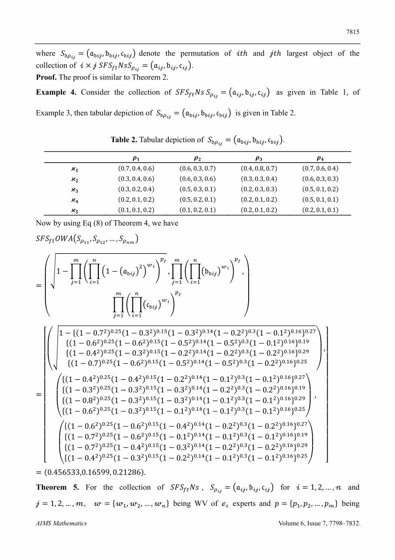
AIMS Mathematics Volume 6, Issue 7, 7798–7832.
where 𝑆𝔡 𝒾𝒿𝔞𝔡𝒾𝒿, 𝔟𝔡𝒾𝒿, 𝔠𝔡𝒾𝒿 denote the permutation of 𝒾𝑡ℎ and 𝒿𝑡ℎ largest object of the
collection of 𝒾 𝒿 𝑆𝐹𝑆 𝑁𝑠𝑆𝒾𝒿
𝔞𝒾𝒿, 𝔟𝒾𝒿, 𝔠𝒾𝒿 .
Proof. The proof is similar to Theorem 2.
Example 4. Consider the collection of 𝑆𝐹𝑆 𝑁𝑠 𝑆𝒾𝒿
𝔞𝒾𝒿, 𝔟𝒾𝒿, 𝔠𝒾𝒿 as given in Table 1, of
Example 3, then tabular depiction of 𝑆𝔡 𝒾𝒿𝔞𝔡𝒾𝒿, 𝔟𝔡𝒾𝒿, 𝔠𝔡𝒾𝒿 is given in Table 2.
Table 2. Tabular depiction of 𝑆𝔡 𝒾𝒿𝔞𝔡𝒾𝒿, 𝔟𝔡𝒾𝒿, 𝔠𝔡𝒾𝒿 .
𝝆𝟏 𝝆𝟐 𝝆𝟑 𝝆𝟒
𝝒𝟏 0.7, 0.4, 0.6 0.6, 0.3, 0.7 0.4, 0.8, 0.7 0.7, 0.6, 0.4
𝝒𝟐 0.3, 0.4, 0.6 0.6, 0.3, 0.6 0.3, 0.3, 0.4 0.6, 0.3, 0.3
𝝒𝟑 0.3, 0.2, 0.4 0.5, 0.3, 0.1 0.2, 0.3, 0.3 0.5, 0.1, 0.2
𝝒𝟒 0.2, 0.1, 0.2 0.5, 0.2, 0.1 0.2, 0.1, 0.2 0.5, 0.1, 0.1
𝝒𝟓 0.1, 0.1, 0.2 0.1, 0.2, 0.1 0.2, 0.1, 0.2 0.2, 0.1, 0.1
Now by using Eq (8) of Theorem 4, we have
𝑆𝐹𝑆 𝑂𝑊𝐴 𝑆 , 𝑆 , … , 𝑆𝓃𝓂
⎝
⎜⎜⎜⎛ 1 1 𝔞𝔡𝒾𝒿
𝓌𝒾𝓃
𝒾
𝒿𝓂
𝒿
, 𝔟𝔡𝒾𝒿𝓌𝒾
𝓃
𝒾
𝒿𝓂
𝒿
,
𝔠𝔡𝒾𝒿𝓌𝒾
𝓃
𝒾
𝒿𝓂
𝒿 ⎠
⎟⎟⎟⎞
⎣⎢⎢⎢⎢⎢⎢⎢⎢⎢⎢⎢⎢⎢⎢⎡
⎝
⎜⎛
1 1 0.7 . 1 0.3 . 1 0.3 . 1 0.2 . 1 0.1 . .
1 0.6 . 1 0.6 . 1 0.5 . 1 0.5 . 1 0.1 . .
1 0.4 . 1 0.3 . 1 0.2 . 1 0.2 . 1 0.2 . .
1 0.7 . 1 0.6 . 1 0.5 . 1 0.5 . 1 0.2 . .⎠
⎟⎞
,
⎝
⎜⎛
1 0.4 . 1 0.4 . 1 0.2 . 1 0.1 . 1 0.1 . .
1 0.3 . 1 0.3 . 1 0.3 . 1 0.2 . 1 0.2 . .
1 0.8 . 1 0.3 . 1 0.3 . 1 0.1 . 1 0.1 . .
1 0.6 . 1 0.3 . 1 0.1 . 1 0.1 . 1 0.1 . .⎠
⎟⎞
,
⎝
⎜⎛
1 0.6 . 1 0.6 . 1 0.4 . 1 0.2 . 1 0.2 . .
1 0.7 . 1 0.6 . 1 0.1 . 1 0.1 . 1 0.1 . .
1 0.7 . 1 0.4 . 1 0.3 . 1 0.2 . 1 0.2 . .
1 0.4 . 1 0.3 . 1 0.2 . 1 0.1 . 1 0.1 . .⎠
⎟⎞
⎦⎥⎥⎥⎥⎥⎥⎥⎥⎥⎥⎥⎥⎥⎥⎤
0.456533,0.16599, 0.21286 .
Theorem 5. For the collection of 𝑆𝐹𝑆 𝑁𝑠 , 𝑆𝒾𝒿
𝔞𝒾𝒿, 𝔟𝒾𝒿, 𝔠𝒾𝒿 for 𝒾 1, 2, … , 𝓃 and
𝒿 1, 2, … , 𝓂, 𝓌 𝓌 , 𝓌 , … , 𝓌𝓃 being WV of ℯ𝒾 experts and 𝑝 𝑝 , 𝑝 , … , 𝑝𝓂 being
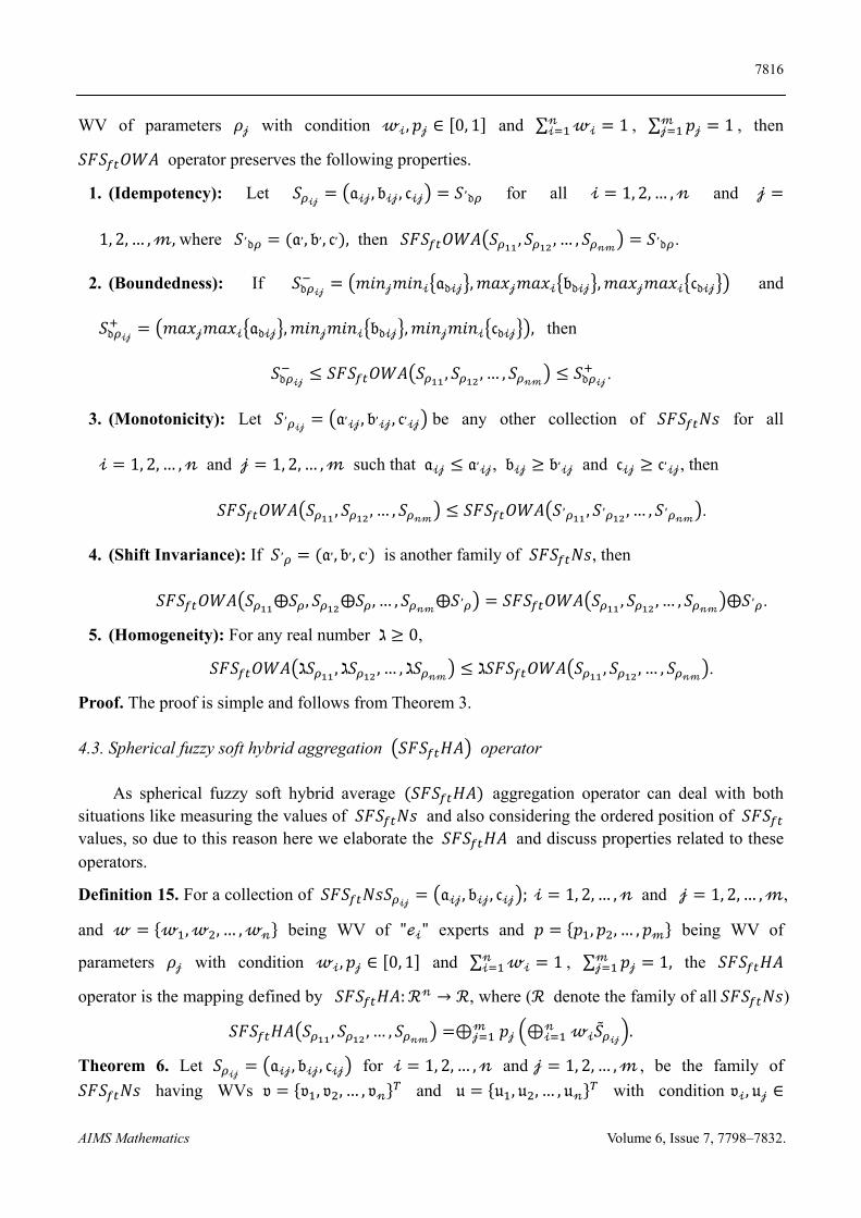
7816
AIMS Mathematics Volume 6, Issue 7, 7798–7832.
WV of parameters 𝜌𝒿 with condition 𝓌𝒾, 𝑝𝒿 ∈ 0, 1 and ∑ 𝓌𝒾 1𝓃𝒾 , ∑ 𝑝𝒿 1𝓂
𝒿 , then
𝑆𝐹𝑆 𝑂𝑊𝐴 operator preserves the following properties.
1. (Idempotency): Let 𝑆𝒾𝒿
𝔞𝒾𝒿, 𝔟𝒾𝒿, 𝔠𝒾𝒿 𝑆,𝔡 for all 𝒾 1, 2, … , 𝓃 and 𝒿
1, 2, … , 𝓂, where 𝑆,𝔡 𝔞,, 𝔟,, 𝔠, , then 𝑆𝐹𝑆 𝑂𝑊𝐴 𝑆 , 𝑆 , … , 𝑆
𝓃𝓂𝑆,
𝔡 .
2. (Boundedness): If 𝑆𝔡 𝒾𝒿𝑚𝑖𝑛𝒿𝑚𝑖𝑛𝒾 𝔞𝔡𝒾𝒿 , 𝑚𝑎𝑥𝒿𝑚𝑎𝑥𝒾 𝔟𝔡𝒾𝒿 , 𝑚𝑎𝑥𝒿𝑚𝑎𝑥𝒾 𝔠𝔡𝒾𝒿 and
𝑆𝔡 𝒾𝒿𝑚𝑎𝑥𝒿𝑚𝑎𝑥𝒾 𝔞𝔡𝒾𝒿 , 𝑚𝑖𝑛𝒿𝑚𝑖𝑛𝒾 𝔟𝔡𝒾𝒿 , 𝑚𝑖𝑛𝒿𝑚𝑖𝑛𝒾 𝔠𝔡𝒾𝒿 , then
𝑆𝔡 𝒾𝒿𝑆𝐹𝑆 𝑂𝑊𝐴 𝑆 , 𝑆 , … , 𝑆
𝓃𝓂𝑆𝔡 𝒾𝒿
.
3. (Monotonicity): Let 𝑆,𝒾𝒿
𝔞,𝒾𝒿, 𝔟,
𝒾𝒿, 𝔠,𝒾𝒿 be any other collection of 𝑆𝐹𝑆 𝑁𝑠 for all
𝒾 1, 2, … , 𝓃 and 𝒿 1, 2, … , 𝓂 such that 𝔞𝒾𝒿 𝔞,𝒾𝒿, 𝔟𝒾𝒿 𝔟,
𝒾𝒿 and 𝔠𝒾𝒿 𝔠,𝒾𝒿, then
𝑆𝐹𝑆 𝑂𝑊𝐴 𝑆 , 𝑆 , … , 𝑆𝓃𝓂
𝑆𝐹𝑆 𝑂𝑊𝐴 𝑆, , 𝑆, , … , 𝑆,𝓃𝓂
.
4. (Shift Invariance): If 𝑆, 𝔞,, 𝔟,, 𝔠, is another family of 𝑆𝐹𝑆 𝑁𝑠, then
𝑆𝐹𝑆 𝑂𝑊𝐴 𝑆 ⨁𝑆 , 𝑆 ⨁𝑆 , … , 𝑆𝓃𝓂
⨁𝑆, 𝑆𝐹𝑆 𝑂𝑊𝐴 𝑆 , 𝑆 , … , 𝑆𝓃𝓂
⨁𝑆, .
5. (Homogeneity): For any real number ℷ 0,
𝑆𝐹𝑆 𝑂𝑊𝐴 ℷ𝑆 , ℷ𝑆 , … , ℷ𝑆𝓃𝓂
ℷ𝑆𝐹𝑆 𝑂𝑊𝐴 𝑆 , 𝑆 , … , 𝑆𝓃𝓂
.
Proof. The proof is simple and follows from Theorem 3.
4.3. Spherical fuzzy soft hybrid aggregation 𝑆𝐹𝑆 𝐻𝐴 operator
As spherical fuzzy soft hybrid average 𝑆𝐹𝑆 𝐻𝐴 aggregation operator can deal with both situations like measuring the values of 𝑆𝐹𝑆 𝑁𝑠 and also considering the ordered position of 𝑆𝐹𝑆 values, so due to this reason here we elaborate the 𝑆𝐹𝑆 𝐻𝐴 and discuss properties related to these operators.
Definition 15. For a collection of 𝑆𝐹𝑆 𝑁𝑠𝑆𝒾𝒿
𝔞𝒾𝒿, 𝔟𝒾𝒿, 𝔠𝒾𝒿 ; 𝒾 1, 2, … , 𝓃 and 𝒿 1, 2, … , 𝓂,
and 𝓌 𝓌 , 𝓌 , … , 𝓌𝓃 being WV of "ℯ𝒾" experts and 𝑝 𝑝 , 𝑝 , … , 𝑝𝓂 being WV of
parameters 𝜌𝒿 with condition 𝓌𝒾, 𝑝𝒿 ∈ 0, 1 and ∑ 𝓌𝒾 1𝓃𝒾 , ∑ 𝑝𝒿 1𝓂
𝒿 , the 𝑆𝐹𝑆 𝛨𝐴
operator is the mapping defined by 𝑆𝐹𝑆 𝛨𝐴: ℛ𝓃 → ℛ, where (ℛ denote the family of all 𝑆𝐹𝑆 𝑁𝑠)
𝑆𝐹𝑆 𝛨𝐴 𝑆 , 𝑆 , … , 𝑆𝓃𝓂
⊕𝒿𝓂 𝑝𝒿 ⊕𝒾
𝓃 𝓌𝒾𝑆𝒾𝒿
.
Theorem 6. Let 𝑆𝒾𝒿
𝔞𝒾𝒿, 𝔟𝒾𝒿, 𝔠𝒾𝒿 for 𝒾 1, 2, … , 𝓃 and 𝒿 1, 2, … , 𝓂 , be the family of
𝑆𝐹𝑆 𝑁𝑠 having WVs 𝔳 𝔳 , 𝔳 , … , 𝔳𝓃 and 𝔲 𝔲 , 𝔲 , … , 𝔲𝓃 with condition 𝔳𝒾, 𝔲𝒿 ∈
7817
AIMS Mathematics Volume 6, Issue 7, 7798–7832.
0, 1 , ∑ 𝔳𝒾 1𝓃𝒾 , ∑ 𝔲𝒿 1𝓂
𝒿 . Also "𝓃" represents the corresponding coefficient for the number
of elements in 𝒾𝑡ℎ row and 𝒿𝑡ℎ column with WVs 𝓌 𝓌 , 𝓌 , … , 𝓌𝓃 denote the WVs of "ℯ𝒾" experts and 𝑝 𝑝 , 𝑝 , … , 𝑝𝓂 being WVs of parameters "𝜌𝒿" with condition 𝓌𝒾, 𝑝𝒿 ∈0, 1 , ∑ 𝓌𝒾 1 𝑎𝑛𝑑 𝓃
𝒾 ∑ 𝑝𝒿 1𝓂𝒿 , then
𝑆𝐹𝑆 𝛨𝐴 𝑆 , 𝑆 , … , 𝑆𝓃𝓂
⊕𝒿𝓂 𝑝𝒿 ⊕𝒾
𝓃 𝓌𝒾𝑆𝒾𝒿
1 ∏ ∏ 1 𝔞𝒾𝒿
𝓌𝒾𝓃𝒾
𝒿𝓂𝒿 , ∏ ∏ 𝔟𝒾𝒿
𝓌𝒾𝓃𝒾
𝒿𝓂𝒿 ,
∏ ∏ �̃�𝒾𝒿𝓌𝒾𝓃
𝒾𝒿𝓂
𝒿
(9)
where 𝑆𝒾𝒿
𝓃𝔳𝒾𝔲𝒿𝑆𝒾𝒿
denote the permutation of 𝒾𝑡ℎ and 𝒿𝑡ℎ largest object of the family of
𝒾 𝒿 𝑆𝐹𝑆𝑁𝑠𝑆𝒾𝒿
𝔞𝒾𝒿, 𝔟𝒾𝒿, �̃�𝒾𝒿 .
Proof. The proof is similar to Theorem 1.
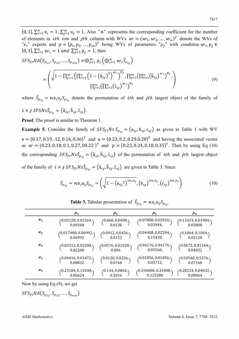
Example 5. Consider the family of 𝑆𝐹𝑆 𝑁𝑠 𝑆𝒾𝒿
𝔞𝒾𝒿, 𝔟𝒾𝒿, 𝔠𝒾𝒿 as given in Table 1 with WV
𝔳 0.17, 0.19, .12, 0.16, 0.36 and 𝔲 0.23, 0.2, 0.29,0.28 and having the associated vector as 𝓌 0.23, 0.18, 0.1, 0.27, 00.22 and 𝑝 0.23, 0.24, 0.18, 0.35 . Then by using Eq (10)
the corresponding 𝑆𝐹𝑆 𝑁𝑠𝑆𝒾𝒿
𝔞𝒾𝒿, 𝔟𝒾𝒿, �̃�𝒾𝒿 of the permutation of 𝒾𝑡ℎ and 𝒿𝑡ℎ largest object
of the family of 𝒾 𝒿 𝑆𝐹𝑆 𝑁𝑠𝑆𝒾𝒿
𝔞𝒾𝒿, 𝔟𝒾𝒿, �̃�𝒾𝒿 are given in Table 3. Since
𝑆𝒾𝒿
𝓃𝔳𝒾𝔲𝒿𝑆𝒾𝒿
1 𝔞𝒾𝒿𝓃𝔳𝒾𝔲𝒿 , 𝔟𝒾𝒿
𝓃𝔳𝒾𝔲𝒿 , 𝔠𝒾𝒿𝓃𝔳𝒾𝔲𝒿 . (10)
Table 3. Tabular presentation of 𝑆𝒾𝒿
𝓃𝔳𝒾𝔲𝒿𝑆𝒾𝒿
.
𝝆𝟏 𝝆𝟐 𝝆𝟑 𝝆𝟒
𝝒𝟏 0.03128, 0.01564, 0.09348
0.068, 0.0408,0.0136
0.07888, 0.05916,
0.03944, 0.11424, 0.01904, 0.03808
𝝒𝟐 0.017480, 0.06992, 0.06992
0.0912, 0.0456,0.0152
0.04408, 0.02204,
0.15428, 0.1064, 0.1064, 0.02128
𝝒𝟑 0.03312, 0.02208, 0.02208
0.0576, 0.01920,0.096
0.04176, 0.04176,
0.05568, 0.0672, 0.01344, 0.04032
𝝒𝟒 0.04416, 0.01472, 0.08832
0.0128, 0.0256,0.0768
0.01856, 0.01856,
0.03712, 0.03548, 0.5376, 0.07168
𝝒𝟓 0.23184, 0.13248, 0.06624
0.144, 0.0864,0.2016
0.334008, 0.33408,0.125280
0.28224, 0.04032, 0.08064
Now by using Eq (9), we get
𝑆𝐹𝑆 𝛨𝐴 𝑆 , 𝑆 , … , 𝑆𝓃𝓂
7818
AIMS Mathematics Volume 6, Issue 7, 7798–7832.
⎝
⎜⎜⎜⎛ 1 1 𝔞𝒾𝒿
𝓌𝒾𝓃
𝒾
𝒿𝓂
𝒿
, 𝔟𝒾𝒿𝓌𝒾
𝓃
𝒾
𝒿𝓂
𝒿
,
�̃�𝒾𝒿𝓌𝒾
𝓃
𝒾
𝒿𝓂
𝒿 ⎠
⎟⎟⎟⎞
0.114201, 0.025752, 0.034869 .
Theorem 7. Let 𝑆𝒾𝒿
𝔞𝒾𝒿, 𝔟𝒾𝒿, 𝔠𝒾𝒿 for 𝒾 1, 2, … , 𝓃 and 𝒿 1, 2, … , 𝓂 , be the family of
𝑆𝐹𝑆 𝑁𝑠 with WVs 𝔳 𝔳 , 𝔳 , … , 𝔳𝓃 and 𝔲 𝔲 , 𝔲 , … , 𝔲𝓃 having condition 𝔳𝒾, 𝔲𝒿 ∈0, 1 and ∑ 𝔳𝒾 1𝓃
𝒾 , ∑ 𝔲𝒿 1𝓂𝒿 . Also "𝓃" represents the corresponding coefficient for the
number of elements in 𝒾𝑡ℎ row and 𝒿𝑡ℎ column linked with vectors 𝓌 𝓌 , 𝓌 , … , 𝓌𝓃 denote the WV of "ℯ𝒾" experts and 𝑝 𝑝 , 𝑝 , … , 𝑝𝓂 denote the WV of parameters "𝜌𝒿" having condition 𝓌𝒾, 𝑝𝒿 ∈ 0, 1 and ∑ 𝓌𝒾 1𝓃
𝒾 , ∑ 𝑝𝒿 1𝓂𝒿 . Then 𝑆𝐹𝑆 𝛨𝐴 operator
contains the subsequent properties:
1. (Idempotency): Let 𝑆𝒾𝒿
𝑆, for all 𝒾 1, 2, … , 𝓃 and 𝒿 1, 2, … , 𝓂,𝑆, 𝓃𝔳𝒾𝔲𝒿𝑆, then
𝑆𝐹𝑆 𝛨𝐴 𝑆 , 𝑆 , … , 𝑆𝓃𝓂
𝑆, .
2. (Boundedness): If 𝑆𝒾𝒿
𝑚𝑖𝑛𝒿𝑚𝑖𝑛𝒾 𝔞𝒾𝒿 , 𝑚𝑎𝑥𝒿𝓂𝑎𝜘𝒾 𝔟𝒾𝒿 , 𝑚𝑎𝑥𝒿𝑚𝑎𝑥𝒾 �̃�𝒾𝒿 and 𝑆𝒾𝒿
𝑚𝑎𝑥𝒿𝑚𝑎𝑥𝒾 𝔞𝒾𝒿 , 𝑚𝑖𝑛𝒿𝑚𝑖𝑛𝒾 𝔟𝒾𝒿 , 𝑚𝑖𝑛𝒿𝑚𝑖𝑛𝒾 �̃�𝒾𝒿 , then
𝑆𝒾𝒿
𝑆𝐹𝑆 𝛨𝐴 𝑆 , 𝑆 , … , 𝑆𝓃𝓂
𝑆𝒾𝒿
.
3. (Monotonicity): Let 𝑆,𝒾𝒿
𝔞,𝒾𝒿, 𝔟,
𝒾𝒿, 𝔠,𝒾𝒿 be any other family of 𝑆𝐹𝑆 𝑁𝑠 for all 𝒾
1, 2, … , 𝓃 and 𝒿 1, 2, … , 𝓂 such that 𝔞𝒾𝒿 𝔞,𝒾𝒿, 𝔟𝒾𝒿 𝔟,
𝒾𝒿 and 𝔠𝒾𝒿 𝔠,𝒾𝒿, then
𝑆𝐹𝑆 𝛨𝐴 𝑆 , 𝑆 , … , 𝑆𝓃𝓂
𝑆𝐹𝑆 𝛨𝐴 𝑆, , 𝑆, , … , 𝑆,𝓃𝓂
.
4. (Shift Invariance): If 𝑆, 𝔞,, 𝔟,, 𝔠, is another family of 𝑆𝐹𝑆 𝑁𝑠, then
𝑆𝐹𝑆 𝛨𝐴 𝑆 ⨁𝑆 , 𝑆 ⨁𝑆 , … , 𝑆𝓃𝓂
⨁𝑆, 𝑆𝐹𝑆 𝛨𝐴 𝑆 , 𝑆 , … , 𝑆𝓃𝓂
⨁𝑆, .
5. (Homogeneity): For any real number ℷ 0,
𝑆𝐹𝑆 𝐻𝐴 ℷ𝑆 , ℷ𝑆 , … , ℷ𝑆𝓃𝓂
ℷ𝑆𝐹𝑆 𝐻𝐴 𝑆 , 𝑆 , … , 𝑆𝓃𝓂
.
Proof. The proof is simple and follows from Theorem 3.
5. A multicriteria decision making method based on spherical fuzzy soft average aggregation operators
In this section, we will discuss a new MCDM method based on 𝑆𝐹𝑆 𝑊𝐴, 𝑆𝐹𝑆 𝑂𝑊𝐴 and
7819
AIMS Mathematics Volume 6, Issue 7, 7798–7832.
𝑆𝐹𝑆 𝐻𝐴 aggregation operators to solve MCDM problems under the environment of 𝑆𝐹𝑆 𝑁𝑠. Consider a common MCDM problem. Let 𝐴 𝜘 , 𝜘 , 𝜘 , … , 𝜘 be the set of "𝑟" alternative,
𝐸 𝐸 , 𝐸 , 𝐸 , … , 𝐸𝓃 be the family of "𝓃" senior experts with 𝜌 𝜌 , 𝜌 , 𝜌 , … , 𝜌𝓂 as a family of "𝓂" parameters. The experts evaluate each alternative 𝜘 𝑙 1, 2, 3, … , 𝑟 according to their respective parameters 𝜌𝒿 𝒿 1, 2, 3, … , 𝓂 . Suppose evaluation information given by experts
is in the form of 𝑆𝐹𝑆 𝑁𝑠 𝑆𝒾𝒿
𝔞𝒾𝒿, 𝔟𝒾𝒿, 𝔠𝒾𝒿 for 𝒾 1, 2, … , 𝓃 and 𝒿 1, 2, … , 𝓂. Let
𝓌 𝓌 , 𝓌 , … , 𝓌𝓃 denote the WV of "ℯ𝒾" experts and 𝑝 𝑝 , 𝑝 , … , 𝑝𝓂 represent the WV of parameters "𝜌𝒿" with a condition that 𝓌𝒾, 𝑝𝒿 ∈ 0, 1 and∑ 𝓌𝒾 1𝓃
𝒾 ,∑ 𝑝𝒿 1.𝓂𝒾 The
overall information is given in matrix 𝑀 𝑆𝒾𝒿 𝓃 𝓂
. By using the aggregation operator for
assessment values, the aggregated 𝑆𝐹𝑆 𝑁 "𝔅 " for alternative 𝜘 𝑙 1, 2, 3, … , 𝑟 are given by 𝔅 𝔞 , 𝔟 , 𝔠 𝑙 1, 2, … , 𝑟 . Use the Definition 10 to find the score values for 𝑆𝐹𝑆 𝑁𝑠 and rank them.
Step vise algorithm is given by Step 1: Arrange all assessment information given by experts for each alternative to their
corresponding parameters to construct an overall decision matrix 𝑀 𝑆𝒾𝒿 𝓃 𝓂
given by:
𝑀
⎣⎢⎢⎢⎡
𝔞 , 𝔟 , 𝔠 𝔞 , 𝔟 , 𝔠 ⋯ 𝔞 𝓂, 𝔟 𝓂, 𝔠 𝓂
𝔞 , 𝔟 , 𝔠⋮
𝔞 , 𝔟 , 𝔠 … 𝔞 𝓂, 𝔟 𝓂, 𝔠 𝓂
𝔞𝓃 , 𝔟𝓃 , 𝔠𝓃⋮
𝔞𝓃 , 𝔟𝓃 , 𝔠𝓃 … 𝔞𝓃𝓂, 𝔟𝓃𝓂, 𝔠𝓃𝓂 ⎦⎥⎥⎥⎤
.
Step 2: Normalize the 𝑆𝐹𝑆 decision matrix that is given in step 1, because there are two type of parameters, cost type parameters and benefit type parameters if it is needed according to the following formula
𝜌𝒾𝒿
𝑆𝒾𝒿
, for cost tyρe parameter
𝑆𝒾𝒿
, for a bene it type parameter
where 𝑆𝒾𝒿
𝔠𝒾𝒿, 𝔟𝒾𝒿, 𝔞𝒾𝒿 denote the complement of 𝑆𝒾𝒿
𝔞𝒾𝒿, 𝔟𝒾𝒿, 𝔠𝒾𝒿 .
Step 3: Aggregate 𝑆𝐹𝑆 𝑁𝑠 by using the proposed aggregation operators for each parameter 𝜌 𝑙 1, 2, … , 𝑟 to get 𝔅 𝔞 , 𝔟 , 𝔠 .
Step 4: Using Definition 10 to calculate the score values for each "𝔅 ".
Step 5: Rank the results for each alternative 𝜘 𝑙 1, 2, 3, … , 𝑟 and choose the best result.
5.1. Application steps for the proposed method
In this section, we describe the detailed explanation of the above-given algorithm through an illustrative example to show the effectiveness of the established work.
Example 6. Suppose a person wants to select the best tyre brand from a set of four alternatives 𝐴𝜘 𝐵𝑟𝑖𝑑𝑔𝑒𝑠𝑡𝑜𝑛𝑒, 𝜘 𝐻𝑎𝑛𝑘𝑜𝑜𝑘, 𝜘 𝐷𝑢𝑛𝑙𝑜𝑝, 𝜘 𝑀𝑅𝐹 𝑡𝑦𝑟𝑒𝑠 . Let a team of experts
consisting of five members 𝐸 𝐸 , 𝐸 , 𝐸 , 𝐸 , 𝐸 with WVs 𝓌 0.15, 0.13, 0.25, 0.23, 0.24 provide their information about alternatives having parameters 𝜌 𝜌 𝐶𝑜𝑟𝑛𝑒𝑟𝑖𝑛𝑔 𝑔𝑟𝑖𝑝, 𝜌
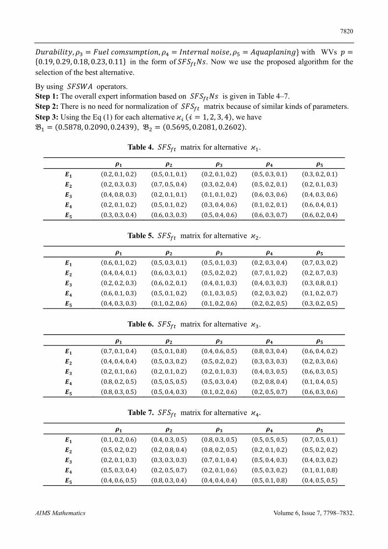
7820
AIMS Mathematics Volume 6, Issue 7, 7798–7832.
𝐷𝑢𝑟𝑎𝑏𝑖𝑙𝑖𝑡𝑦, 𝜌 𝐹𝑢𝑒𝑙 𝑐𝑜𝑚𝑠𝑢𝑚𝑝𝑡𝑖𝑜𝑛, 𝜌 𝐼𝑛𝑡𝑒𝑟𝑛𝑎𝑙 𝑛𝑜𝑖𝑠𝑒, 𝜌 𝐴𝑞𝑢𝑎𝑝𝑙𝑎𝑛𝑖𝑛𝑔 with WVs 𝑝0.19, 0.29, 0.18, 0.23, 0.11 in the form of 𝑆𝐹𝑆 𝑁𝑠. Now we use the proposed algorithm for the
selection of the best alternative.
By using 𝑆𝐹𝑆𝑊𝐴 operators. Step 1: The overall expert information based on 𝑆𝐹𝑆 𝑁𝑠 is given in Table 4–7. Step 2: There is no need for normalization of 𝑆𝐹𝑆 matrix because of similar kinds of parameters. Step 3: Using the Eq (1) for each alternative 𝜘𝒾 𝒾 1, 2, 3, 4 , we have 𝔅 0.5878, 0.2090, 0.2439 , 𝔅 0.5695, 0.2081, 0.2602 .
Table 4. 𝑆𝐹𝑆 matrix for alternative 𝜘 .
𝝆𝟏 𝝆𝟐 𝝆𝟑 𝝆𝟒 𝝆𝟓
𝑬𝟏 0.2, 0.1, 0.2 0.5, 0.1, 0.1 0.2, 0.1, 0.2 0.5, 0.3, 0.1 0.3, 0.2, 0.1
𝑬𝟐 0.2, 0.3, 0.3 0.7, 0.5, 0.4 0.3, 0.2, 0.4 0.5, 0.2, 0.1 0.2, 0.1, 0.3
𝑬𝟑 0.4, 0.8, 0.3 0.2, 0.1, 0.1 0.1, 0.1, 0.2 0.6, 0.3, 0.6 0.4, 0.3, 0.6
𝑬𝟒 0.2, 0.1, 0.2 0.5, 0.1, 0.2 0.3, 0.4, 0.6 0.1, 0.2, 0.1 0.6, 0.4, 0.1
𝑬𝟓 0.3, 0.3, 0.4 0.6, 0.3, 0.3 0.5, 0.4, 0.6 0.6, 0.3, 0.7 0.6, 0.2, 0.4
Table 5. 𝑆𝐹𝑆 matrix for alternative 𝜘 .
𝝆𝟏 𝝆𝟐 𝝆𝟑 𝝆𝟒 𝝆𝟓
𝑬𝟏 0.6, 0.1, 0.2 0.5, 0.3, 0.1 0.5, 0.1, 0.3 0.2, 0.3, 0.4 0.7, 0.3, 0.2
𝑬𝟐 0.4, 0.4, 0.1 0.6, 0.3, 0.1 0.5, 0.2, 0.2 0.7, 0.1, 0.2 0.2, 0.7, 0.3
𝑬𝟑 0.2, 0.2, 0.3 0.6, 0.2, 0.1 0.4, 0.1, 0.3 0.4, 0.3, 0.3 0.3, 0.8, 0.1
𝑬𝟒 0.6, 0.1, 0.3 0.5, 0.1, 0.2 0.1, 0.3, 0.5 0.2, 0.3, 0.2 0.1, 0.2, 0.7
𝑬𝟓 0.4, 0.3, 0.3 0.1, 0.2, 0.6 0.1, 0.2, 0.6 0.2, 0.2, 0.5 0.3, 0.2, 0.5
Table 6. 𝑆𝐹𝑆 matrix for alternative 𝜘 .
𝝆𝟏 𝝆𝟐 𝝆𝟑 𝝆𝟒 𝝆𝟓
𝑬𝟏 0.7, 0.1, 0.4 0.5, 0.1, 0.8 0.4, 0.6, 0.5 0.8, 0.3, 0.4 0.6, 0.4, 0.2
𝑬𝟐 0.4, 0.4, 0.4 0.5, 0.3, 0.2 0.5, 0.2, 0.2 0.3, 0.3, 0.3 0.2, 0.3, 0.6
𝑬𝟑 0.2, 0.1, 0.6 0.2, 0.1, 0.2 0.2, 0.1, 0.3 0.4, 0.3, 0.5 0.6, 0.3, 0.5
𝑬𝟒 0.8, 0.2, 0.5 0.5, 0.5, 0.5 0.5, 0.3, 0.4 0.2, 0.8, 0.4 0.1, 0.4, 0.5
𝑬𝟓 0.8, 0.3, 0.5 0.5, 0.4, 0.3 0.1, 0.2, 0.6 0.2, 0.5, 0.7 0.6, 0.3, 0.6
Table 7. 𝑆𝐹𝑆 matrix for alternative 𝜘 .
𝝆𝟏 𝝆𝟐 𝝆𝟑 𝝆𝟒 𝝆𝟓
𝑬𝟏 0.1, 0.2, 0.6 0.4, 0.3, 0.5 0.8, 0.3, 0.5 0.5, 0.5, 0.5 0.7, 0.5, 0.1
𝑬𝟐 0.5, 0.2, 0.2 0.2, 0.8, 0.4 0.8, 0.2, 0.5 0.2, 0.1, 0.2 0.5, 0.2, 0.2
𝑬𝟑 0.2, 0.1, 0.3 0.3, 0.3, 0.3 0.7, 0.1, 0.4 0.5, 0.4, 0.3 0.4, 0.3, 0.2
𝑬𝟒 0.5, 0.3, 0.4 0.2, 0.5, 0.7 0.2, 0.1, 0.6 0.5, 0.3, 0.2 0.1, 0.1, 0.8
𝑬𝟓 0.4, 0.6, 0.5 0.8, 0.3, 0.4 0.4, 0.4, 0.4 0.5, 0.1, 0.8 0.4, 0.5, 0.5
7821
AIMS Mathematics Volume 6, Issue 7, 7798–7832.
𝔅 0.6330, 0.2626, 0.4138 , 𝔅 0.6341, 0.2623, 0.3955 .
Step 4: To find out the score values, use Definition 10 for each 𝔅𝒾 𝒾 1, 2, 3, 4, 5 given in step 3, i.e. 𝑆𝑐 𝔅 0.7116, 𝑆𝑐 𝔅 0.7004, 𝑆𝑐 𝔅 0.6522, 𝑆𝑐 𝔅 0.6587.
Step 5: Select the best solution by ranking the score values. 𝑆𝑐 𝔅 𝑆𝑐 𝔅 𝑆𝑐 𝔅 𝑆𝑐 𝔅 .
Hence it is clear that "𝜘 " is the best result.
By using 𝑆𝐹𝑆 𝑂𝑊𝐴 operators. Step 1: Same as above. Step 2: Same as above. Step 3: Using the Eq (8) for each alternative 𝜘𝒾 𝒾 1, 2, 3, 4 , we have
𝔅 0.5670, 0.1843, 0.2113 , 𝔅 0.5601, 0.1936, 0.2211 , 𝔅 0.6145, 0.2379, 0.3771 , 𝔅 0.6098, 0.2433, 0.3591 .
Step 4: To find out the score values, use Definition 10 for each 𝔅𝒾 𝒾 1, 2, 3, 4, 5 given in step 3, i.e. 𝑆𝑐 𝔅 0.7238, 𝑆𝑐 𝔅 0.7151, 𝑆𝑐 𝔅 0.6665, 𝑆𝑐 𝔅 0.6691.
Step 5: Select the best solution by ranking the score values.
𝑆𝑐 𝔅 𝑆𝑐 𝔅 𝑆𝑐 𝔅 𝑆𝑐 𝔅 . Note that the aggregated result for 𝑆𝐹𝑆 𝑂𝑊𝐴 operator is same as result obtained for 𝑆𝐹𝑆 𝑊𝐴 operator. Hence "𝜘 " is the best result.
By using 𝑆𝐹𝑆 𝛨𝐴 operators. Step 1: Same as above. Step 2: Same as above. Step 3: Using the Eq (9) for each alternative𝜘𝒾 𝒾 1, 2, 3, 4 , with 𝔳 0.12, 0.13, 0.2,0.4, 0.15 and 𝔲 0.11, 0.14, 0.2, 0.3, 0.25 being the WVs of 𝑆
𝒾𝒿𝔞𝒾𝒿, 𝔟𝒾𝒿, 𝔠𝒾𝒿 . Also "𝓃" represents
the corresponding balancing coefficient for the number of elements in 𝒾𝑡ℎ row and 𝒿𝑡ℎ column. Let 𝓌 0.15, 0.13, 0.25, 0.23, 0.24 be the WV of "ℯ𝒾" experts and 𝑝 0.19, 0.29, 0.18, 0.23, 0.11 denote the WV of "𝜌𝒿" parameters, so we get
𝔅 0.3823, 0.6357, 0.6422 , 𝔅 0.3801, 0.6379, 0.6411 , 𝔅 0.3579, 0.6347, 0.6645 , 𝔅 0.3616, 0.6454, 0.6567 .
Step 4: To find out the score values, use Definition 10 for each 𝔅𝒾 𝒾 1, 2, 3, 4, 5 given in step 3, i.e. 𝑆𝑐 𝔅 0.3681, 𝑆𝑐 𝔅 0.3670, 𝑆𝑐 𝔅 0.3529, 𝑆𝑐 𝔅 0.3531.
Step 5: Select the best solution by ranking the score values.
𝑆𝑐 𝔅 𝑆𝑐 𝔅 𝑆𝑐 𝔅 𝑆𝑐 𝔅 .
Hence it is noted that the aggregated result for 𝑆𝐹𝑆 𝛨𝐴 operator is same as result obtained for 𝑆𝐹𝑆 𝑊𝐴 and 𝑆𝐹𝑆 𝑂𝑊𝐴 operator. Hence "𝜘 " is the best alternative.
7822
AIMS Mathematics Volume 6, Issue 7, 7798–7832.
5.2. Comparative analysis
In this section, we are desire to establish the comparative analysis of proposed work with some existing operators to discuss the superiority and validity of established work. The overall analysis is captured in the following examples.
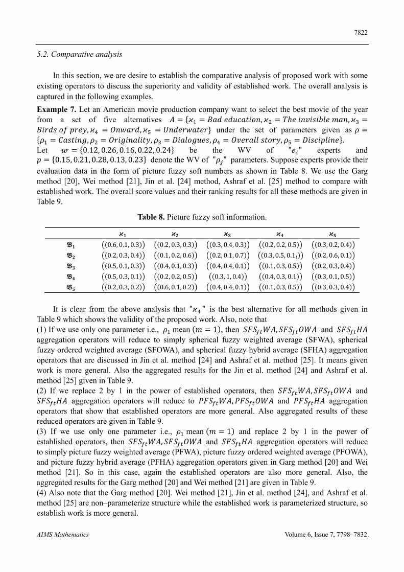
Example 7. Let an American movie production company want to select the best movie of the year from a set of five alternatives 𝐴 𝜘 𝐵𝑎𝑑 𝑒𝑑𝑢𝑐𝑎𝑡𝑖𝑜𝑛, 𝜘 𝑇ℎ𝑒 𝑖𝑛𝑣𝑖𝑠𝑖𝑏𝑙𝑒 𝑚𝑎𝑛, 𝜘𝐵𝑖𝑟𝑑𝑠 𝑜𝑓 𝑝𝑟𝑒𝑦, 𝜘 𝑂𝑛𝑤𝑎𝑟𝑑, 𝜘 𝑈𝑛𝑑𝑒𝑟𝑤𝑎𝑡𝑒𝑟 under the set of parameters given as 𝜌𝜌 𝐶𝑎𝑠𝑡𝑖𝑛𝑔, 𝜌 𝑂𝑟𝑖𝑔𝑖𝑛𝑎𝑙𝑖𝑡𝑦, 𝜌 𝐷𝑖𝑎𝑙𝑜𝑔𝑢𝑒𝑠, 𝜌 𝑂𝑣𝑒𝑟𝑎𝑙𝑙 𝑠𝑡𝑜𝑟𝑦, 𝜌 𝐷𝑖𝑠𝑐𝑖𝑝𝑙𝑖𝑛𝑒 .
Let 𝓌 0.12, 0.26, 0.16, 0.22, 0.24 be the WV of "ℯ𝒾" experts and 𝑝 0.15, 0.21, 0.28, 0.13, 0.23 denote the WV of "𝜌𝒿" parameters. Suppose experts provide their
evaluation data in the form of picture fuzzy soft numbers as shown in Table 8. We use the Garg method [20], Wei method [21], Jin et al. [24] method, Ashraf et al. [25] method to compare with established work. The overall score values and their ranking results for all these methods are given in Table 9.
Table 8. Picture fuzzy soft information.
𝝒𝟏 𝝒𝟐 𝝒𝟑 𝝒𝟒 𝝒𝟓
𝕭𝟏 0.6, 0.1, 0.3 0.2, 0.3, 0.3 0.3, 0.4, 0.3 0.2, 0.2, 0.5 0.3, 0.2, 0.4
𝕭𝟐 0.2, 0.3, 0.4 0.1, 0.2, 0.6 0.2, 0.1, 0.7 0.3, 0.5, 0.1 0.2, 0.6, 0.1
𝕭𝟑 0.5, 0.1, 0.3 0.4, 0.1, 0.3 0.4, 0.4, 0.1 0.1, 0.3, 0.5 0.2, 0.3, 0.4
𝕭𝟒 0.5, 0.3, 0.1 0.2, 0.2, 0.5 0.3, 1, 0.4 0.4, 0.3, 0.1 0.3, 0.1, 0.5
𝕭𝟓 0.2, 0.3, 0.2 0.6, 0.1, 0.2 0.4, 0.4, 0.1 0.1, 0.3, 0.5 0.3, 0.3, 0.4
It is clear from the above analysis that "𝜘 " is the best alternative for all methods given in
Table 9 which shows the validity of the proposed work. Also, note that (1) If we use only one parameter i.e., 𝜌 mean 𝑚 1 , then 𝑆𝐹𝑆 𝑊𝐴, 𝑆𝐹𝑆 𝑂𝑊𝐴 and 𝑆𝐹𝑆 𝐻𝐴 aggregation operators will reduce to simply spherical fuzzy weighted average (SFWA), spherical fuzzy ordered weighted average (SFOWA), and spherical fuzzy hybrid average (SFHA) aggregation operators that are discussed in Jin et al. method [24] and Ashraf et al. method [25]. It means given work is more general. Also the aggregated results for the Jin et al. method [24] and Ashraf et al. method [25] given in Table 9. (2) If we replace 2 by 1 in the power of established operators, then 𝑆𝐹𝑆 𝑊𝐴, 𝑆𝐹𝑆 𝑂𝑊𝐴 and 𝑆𝐹𝑆 𝐻𝐴 aggregation operators will reduce to 𝑃𝐹𝑆 𝑊𝐴, 𝑃𝐹𝑆 𝑂𝑊𝐴 and 𝑃𝐹𝑆 𝐻𝐴 aggregation operators that show that established operators are more general. Also aggregated results of these reduced operators are given in Table 9. (3) If we use only one parameter i.e., 𝜌 mean 𝑚 1 and replace 2 by 1 in the power of established operators, then 𝑆𝐹𝑆 𝑊𝐴, 𝑆𝐹𝑆 𝑂𝑊𝐴 and 𝑆𝐹𝑆 𝐻𝐴 aggregation operators will reduce to simply picture fuzzy weighted average (PFWA), picture fuzzy ordered weighted average (PFOWA), and picture fuzzy hybrid average (PFHA) aggregation operators given in Garg method [20] and Wei method [21]. So in this case, again the established operators are also more general. Also, the aggregated results for the Garg method [20] and Wei method [21] are given in Table 9. (4) Also note that the Garg method [20]. Wei method [21], Jin et al. method [24], and Ashraf et al. method [25] are non–parameterize structure while the established work is parameterized structure, so establish work is more general.
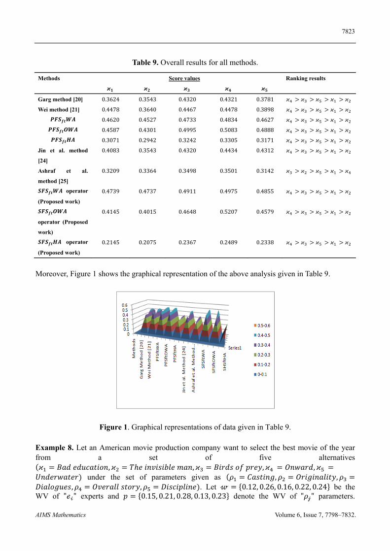
7823
AIMS Mathematics Volume 6, Issue 7, 7798–7832.
Table 9. Overall results for all methods.
Methods
𝝒𝟏
𝝒𝟐
Score values
𝝒𝟑
𝝒𝟒
𝝒𝟓
Ranking results
Garg method [20] 0.3624 0.3543 0.4320 0.4321 0.3781 𝜘 𝜘 𝜘 𝜘 𝜘
Wei method [21] 0.4478 0.3640 0.4467 0.4478 0.3898 𝜘 𝜘 𝜘 𝜘 𝜘
𝑷𝑭𝑺𝒇𝒕𝑾𝑨 0.4620 0.4527 0.4733 0.4834 0.4627 𝜘 𝜘 𝜘 𝜘 𝜘
𝑷𝑭𝑺𝒇𝒕𝑶𝑾𝑨 0.4587 0.4301 0.4995 0.5083 0.4888 𝜘 𝜘 𝜘 𝜘 𝜘
𝑷𝑭𝑺𝒇𝒕𝑯𝑨 0.3071 0.2942 0.3242 0.3305 0.3171 𝜘 𝜘 𝜘 𝜘 𝜘
Jin et al. method
[24]
0.4083 0.3543 0.4320 0.4434 0.4312 𝜘 𝜘 𝜘 𝜘 𝜘
Ashraf et al.
method [25]
0.3209 0.3364 0.3498 0.3501 0.3142 𝜘 𝜘 𝜘 𝜘 𝜘
𝑺𝑭𝑺𝒇𝒕𝑾𝑨 operator
(Proposed work)
0.4739 0.4737 0.4911 0.4975 0.4855 𝜘 𝜘 𝜘 𝜘 𝜘
𝑺𝑭𝑺𝒇𝒕𝑶𝑾𝑨
operator (Proposed
work)
0.4145 0.4015 0.4648 0.5207 0.4579 𝜘 𝜘 𝜘 𝜘 𝜘
𝑺𝑭𝑺𝒇𝒕𝑯𝑨 operator
(Proposed work)
0.2145 0.2075 0.2367 0.2489 0.2338 𝜘 𝜘 𝜘 𝜘 𝜘
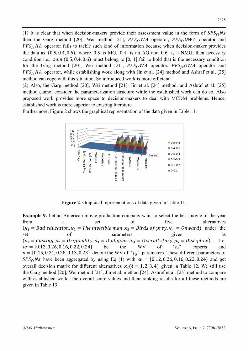
Moreover, Figure 1 shows the graphical representation of the above analysis given in Table 9.
Figure 1. Graphical representations of data given in Table 9.
Example 8. Let an American movie production company want to select the best movie of the year from a set of five alternatives 𝜘 𝐵𝑎𝑑 𝑒𝑑𝑢𝑐𝑎𝑡𝑖𝑜𝑛, 𝜘 𝑇ℎ𝑒 𝑖𝑛𝑣𝑖𝑠𝑖𝑏𝑙𝑒 𝑚𝑎𝑛, 𝜘 𝐵𝑖𝑟𝑑𝑠 𝑜𝑓 𝑝𝑟𝑒𝑦, 𝜘 𝑂𝑛𝑤𝑎𝑟𝑑, 𝜘
𝑈𝑛𝑑𝑒𝑟𝑤𝑎𝑡𝑒𝑟 under the set of parameters given as 𝜌 𝐶𝑎𝑠𝑡𝑖𝑛𝑔, 𝜌 𝑂𝑟𝑖𝑔𝑖𝑛𝑎𝑙𝑖𝑡𝑦, 𝜌𝐷𝑖𝑎𝑙𝑜𝑔𝑢𝑒𝑠, 𝜌 𝑂𝑣𝑒𝑟𝑎𝑙𝑙 𝑠𝑡𝑜𝑟𝑦, 𝜌 𝐷𝑖𝑠𝑐𝑖𝑝𝑙𝑖𝑛𝑒 . Let 𝓌 0.12, 0.26, 0.16, 0.22, 0.24 be the WV of "ℯ𝒾" experts and 𝑝 0.15, 0.21, 0.28, 0.13, 0.23 denote the WV of "𝜌𝒿" parameters.
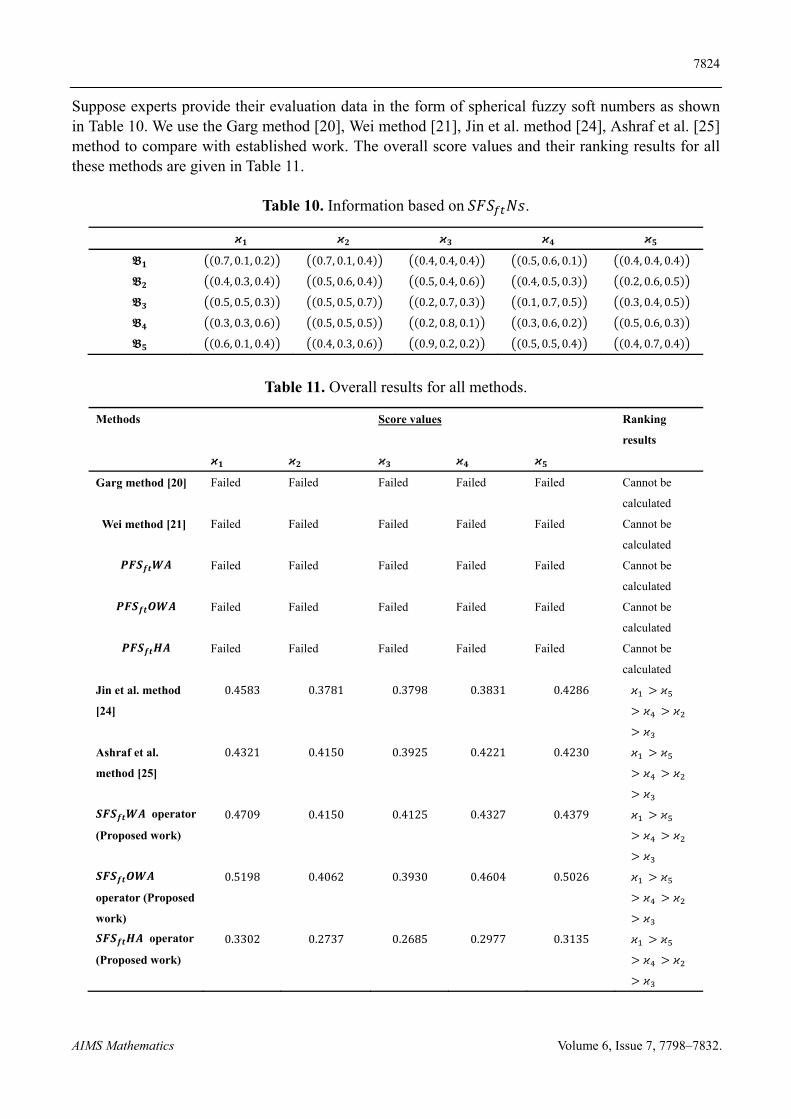
7824
AIMS Mathematics Volume 6, Issue 7, 7798–7832.
Suppose experts provide their evaluation data in the form of spherical fuzzy soft numbers as shown in Table 10. We use the Garg method [20], Wei method [21], Jin et al. method [24], Ashraf et al. [25] method to compare with established work. The overall score values and their ranking results for all these methods are given in Table 11.
Table 10. Information based on 𝑆𝐹𝑆 𝑁𝑠.
𝝒𝟏 𝝒𝟐 𝝒𝟑 𝝒𝟒 𝝒𝟓
𝕭𝟏 0.7, 0.1, 0.2 0.7, 0.1, 0.4 0.4, 0.4, 0.4 0.5, 0.6, 0.1 0.4, 0.4, 0.4
𝕭𝟐 0.4, 0.3, 0.4 0.5, 0.6, 0.4 0.5, 0.4, 0.6 0.4, 0.5, 0.3 0.2, 0.6, 0.5
𝕭𝟑 0.5, 0.5, 0.3 0.5, 0.5, 0.7 0.2, 0.7, 0.3 0.1, 0.7, 0.5 0.3, 0.4, 0.5
𝕭𝟒 0.3, 0.3, 0.6 0.5, 0.5, 0.5 0.2, 0.8, 0.1 0.3, 0.6, 0.2 0.5, 0.6, 0.3
𝕭𝟓 0.6, 0.1, 0.4 0.4, 0.3, 0.6 0.9, 0.2, 0.2 0.5, 0.5, 0.4 0.4, 0.7, 0.4
Table 11. Overall results for all methods.
Methods
𝝒𝟏
𝝒𝟐
Score values
𝝒𝟑
𝝒𝟒
𝝒𝟓
Ranking
results
Garg method [20] Failed Failed Failed Failed Failed Cannot be
calculated
Wei method [21] Failed Failed Failed Failed Failed Cannot be
calculated
𝑷𝑭𝑺𝒇𝒕𝑾𝑨 Failed Failed Failed Failed Failed Cannot be
calculated
𝑷𝑭𝑺𝒇𝒕𝑶𝑾𝑨 Failed Failed Failed Failed Failed Cannot be
calculated
𝑷𝑭𝑺𝒇𝒕𝑯𝑨 Failed Failed Failed Failed Failed Cannot be
calculated
Jin et al. method
[24]
0.4583 0.3781 0.3798 0.3831 0.4286 𝜘 𝜘
𝜘 𝜘
𝜘
Ashraf et al.
method [25]
0.4321 0.4150 0.3925 0.4221 0.4230 𝜘 𝜘
𝜘 𝜘
𝜘
𝑺𝑭𝑺𝒇𝒕𝑾𝑨 operator
(Proposed work)
0.4709 0.4150 0.4125 0.4327 0.4379 𝜘 𝜘
𝜘 𝜘
𝜘
𝑺𝑭𝑺𝒇𝒕𝑶𝑾𝑨
operator (Proposed
work)
0.5198 0.4062 0.3930 0.4604 0.5026 𝜘 𝜘
𝜘 𝜘
𝜘
𝑺𝑭𝑺𝒇𝒕𝑯𝑨 operator
(Proposed work)
0.3302 0.2737 0.2685 0.2977 0.3135 𝜘 𝜘
𝜘 𝜘
𝜘
7825
AIMS Mathematics Volume 6, Issue 7, 7798–7832.
(1) It is clear that when decision-makers provide their assessment value in the form of 𝑆𝐹𝑆 𝑁𝑠 then the Garg method [20], Wei method [21], 𝑃𝐹𝑆 𝑊𝐴 operator, 𝑃𝐹𝑆 𝑂𝑊𝐴 operator and 𝑃𝐹𝑆 𝐻𝐴 operator fails to tackle such kind of information because when decision-maker provides the data as 0.5, 0.4, 0.6 , where 0.5 is MG, 0.4 is an AG and 0.6 is a NMG, then necessary condition i.e., 𝑠𝑢𝑚 0.5, 0.4, 0.6 must belong to [0, 1] fail to hold that is the necessary condition for the Garg method [20], Wei method [21], 𝑃𝐹𝑆 𝑊𝐴 operator, 𝑃𝐹𝑆 𝑂𝑊𝐴 operator and 𝑃𝐹𝑆 𝐻𝐴 operator, while establishing work along with Jin et al. [24] method and Ashraf et al, [25] method can cope with this situation. So introduced work is more efficient. (2) Also, the Garg method [20], Wei method [21], Jin et al. [24] method, and Ashraf et al. [25] method cannot consider the parameterization structure while the established work can do so. Also proposed work provides more space to decision-makers to deal with MCDM problems. Hence, established work is more superior to existing literature. Furthermore, Figure 2 shows the graphical representation of the data given in Table 11.
Figure 2. Graphical representations of data given in Table 11.
Example 9. Let an American movie production company want to select the best movie of the year from a set of five alternatives 𝜘 𝐵𝑎𝑑 𝑒𝑑𝑢𝑐𝑎𝑡𝑖𝑜𝑛, 𝜘 𝑇ℎ𝑒 𝑖𝑛𝑣𝑖𝑠𝑖𝑏𝑙𝑒 𝑚𝑎𝑛, 𝜘 𝐵𝑖𝑟𝑑𝑠 𝑜𝑓 𝑝𝑟𝑒𝑦, 𝜘 𝑂𝑛𝑤𝑎𝑟𝑑 under the
set of parameters given as 𝜌 𝐶𝑎𝑠𝑡𝑖𝑛𝑔, 𝜌 𝑂𝑟𝑖𝑔𝑖𝑛𝑎𝑙𝑖𝑡𝑦, 𝜌 𝐷𝑖𝑎𝑙𝑜𝑔𝑢𝑒𝑠, 𝜌 𝑂𝑣𝑒𝑟𝑎𝑙𝑙 𝑠𝑡𝑜𝑟𝑦, 𝜌 𝐷𝑖𝑠𝑐𝑖𝑝𝑙𝑖𝑛𝑒 . Let
𝓌 0.12, 0.26, 0.16, 0.22, 0.24 be the WV of "ℯ𝒾" experts and 𝑝 0.15, 0.21, 0.28, 0.13, 0.23 denote the WV of "𝜌𝒿" parameters. These different parameters of 𝑆𝐹𝑆 𝑁𝑠 have been aggregated by using Eq (1) with 𝓌 0.12, 0.26, 0.16, 0.22, 0.24 and get overall decision matrix for different alternatives 𝜘𝒾 𝒾 1, 2, 3, 4 given in Table 12. We still use the Garg method [20], Wei method [21], Jin et al. method [24], Ashraf et al. [25] method to compare with established work. The overall score values and their ranking results for all these methods are given in Table 13.
7826
AIMS Mathematics Volume 6, Issue 7, 7798–7832.
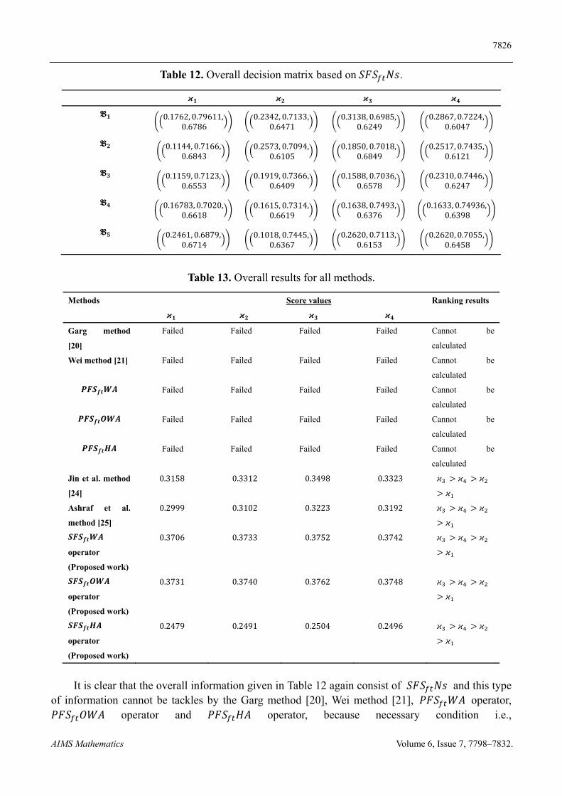
Table 12. Overall decision matrix based on 𝑆𝐹𝑆 𝑁𝑠.
𝝒𝟏 𝝒𝟐 𝝒𝟑 𝝒𝟒
𝕭𝟏 0.1762, 0.79611, 0.6786
0.2342, 0.7133,0.6471
0.3138, 0.6985,0.6249
0.2867, 0.7224, 0.6047
𝕭𝟐 0.1144, 0.7166, 0.6843
0.2573, 0.7094,0.6105
0.1850, 0.7018,0.6849
0.2517, 0.7435, 0.6121
𝕭𝟑 0.1159, 0.7123, 0.6553
0.1919, 0.7366,0.6409
0.1588, 0.7036,0.6578
0.2310, 0.7446, 0.6247
𝕭𝟒 0.16783, 0.7020, 0.6618
0.1615, 0.7314,0.6619
0.1638, 0.7493,0.6376
0.1633, 0.74936, 0.6398
𝕭𝟓 0.2461, 0.6879, 0.6714
0.1018, 0.7445,0.6367
0.2620, 0.7113,0.6153
0.2620, 0.7055, 0.6458
Table 13. Overall results for all methods.
Methods
𝝒𝟏
𝝒𝟐
Score values
𝝒𝟑
𝝒𝟒
Ranking results
Garg method
[20]
Failed Failed Failed Failed Cannot be
calculated
Wei method [21] Failed Failed Failed Failed Cannot be
calculated
𝑷𝑭𝑺𝒇𝒕𝑾𝑨 Failed Failed Failed Failed Cannot be
calculated
𝑷𝑭𝑺𝒇𝒕𝑶𝑾𝑨 Failed Failed Failed Failed Cannot be
calculated
𝑷𝑭𝑺𝒇𝒕𝑯𝑨 Failed Failed Failed Failed Cannot be
calculated
Jin et al. method
[24]
0.3158 0.3312 0.3498 0.3323 𝜘 𝜘 𝜘
𝜘
Ashraf et al.
method [25]
0.2999 0.3102 0.3223 0.3192 𝜘 𝜘 𝜘
𝜘
𝑺𝑭𝑺𝒇𝒕𝑾𝑨
operator
(Proposed work)
0.3706 0.3733 0.3752 0.3742 𝜘 𝜘 𝜘
𝜘
𝑺𝑭𝑺𝒇𝒕𝑶𝑾𝑨
operator
(Proposed work)
0.3731 0.3740 0.3762 0.3748 𝜘 𝜘 𝜘
𝜘
𝑺𝑭𝑺𝒇𝒕𝑯𝑨
operator
(Proposed work)
0.2479 0.2491 0.2504 0.2496 𝜘 𝜘 𝜘
𝜘
It is clear that the overall information given in Table 12 again consist of 𝑆𝐹𝑆 𝑁𝑠 and this type
of information cannot be tackles by the Garg method [20], Wei method [21], 𝑃𝐹𝑆 𝑊𝐴 operator, 𝑃𝐹𝑆 𝑂𝑊𝐴 operator and 𝑃𝐹𝑆 𝐻𝐴 operator, because necessary condition i.e.,
7827
AIMS Mathematics Volume 6, Issue 7, 7798–7832.
𝑠𝑢𝑚 0.1919, 0.7366, 0.6409 fail to hold for all above-given methods for the data 0.1919, 0.7366,
0.6409 given in Table 12, while established work can handle this kind of information.
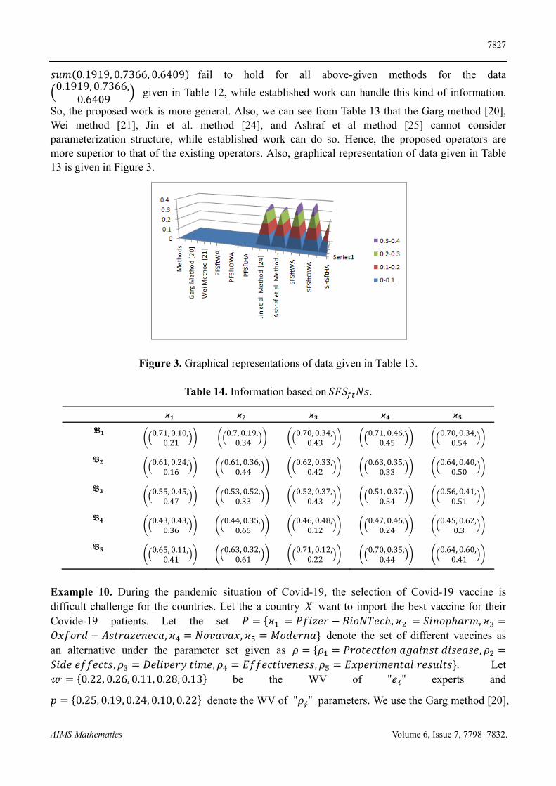
So, the proposed work is more general. Also, we can see from Table 13 that the Garg method [20], Wei method [21], Jin et al. method [24], and Ashraf et al method [25] cannot consider parameterization structure, while established work can do so. Hence, the proposed operators are more superior to that of the existing operators. Also, graphical representation of data given in Table 13 is given in Figure 3.
Figure 3. Graphical representations of data given in Table 13.
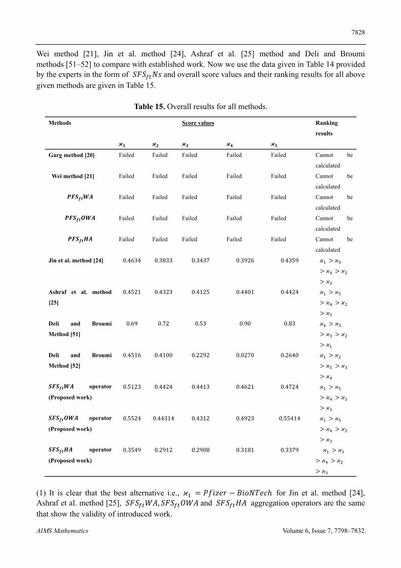
Table 14. Information based on 𝑆𝐹𝑆 𝑁𝑠.
𝝒𝟏 𝝒𝟐 𝝒𝟑 𝝒𝟒 𝝒𝟓
𝕭𝟏 0.71, 0.10, 0.21
0.7, 0.19,0.34
0.70, 0.34,0.43
0.71, 0.46,0.45
0.70, 0.34, 0.54
𝕭𝟐 0.61, 0.24, 0.16
0.61, 0.36,0.44
0.62, 0.33,0.42
0.63, 0.35,0.33
0.64, 0.40, 0.50
𝕭𝟑 0.55, 0.45, 0.47
0.53, 0.52,0.33
0.52, 0.37,0.43
0.51, 0.37,0.54
0.56, 0.41, 0.51
𝕭𝟒 0.43, 0.43, 0.36
0.44, 0.35,0.65
0.46, 0.48,0.12
0.47, 0.46,0.24
0.45, 0.62, 0.3
𝕭𝟓 0.65, 0.11, 0.41
0.63, 0.32,0.61
0.71, 0.12,0.22
0.70, 0.35,0.44
0.64, 0.60, 0.41
Example 10. During the pandemic situation of Covid-19, the selection of Covid-19 vaccine is difficult challenge for the countries. Let the a country 𝑋 want to import the best vaccine for their Covide-19 patients. Let the set 𝑃 𝜘 𝑃𝑓𝑖𝑧𝑒𝑟 𝐵𝑖𝑜𝑁𝑇𝑒𝑐ℎ, 𝜘 𝑆𝑖𝑛𝑜𝑝ℎ𝑎𝑟𝑚, 𝜘𝑂𝑥𝑓𝑜𝑟𝑑 𝐴𝑠𝑡𝑟𝑎𝑧𝑒𝑛𝑒𝑐𝑎, 𝜘 𝑁𝑜𝑣𝑎𝑣𝑎𝑥, 𝜘 𝑀𝑜𝑑𝑒𝑟𝑛𝑎 denote the set of different vaccines as an alternative under the parameter set given as 𝜌 𝜌 𝑃𝑟𝑜𝑡𝑒𝑐𝑡𝑖𝑜𝑛 𝑎𝑔𝑎𝑖𝑛𝑠𝑡 𝑑𝑖𝑠𝑒𝑎𝑠𝑒, 𝜌𝑆𝑖𝑑𝑒 𝑒𝑓𝑓𝑒𝑐𝑡𝑠, 𝜌 𝐷𝑒𝑙𝑖𝑣𝑒𝑟𝑦 𝑡𝑖𝑚𝑒, 𝜌 𝐸𝑓𝑓𝑒𝑐𝑡𝑖𝑣𝑒𝑛𝑒𝑠𝑠, 𝜌 𝐸𝑥𝑝𝑒𝑟𝑖𝑚𝑒𝑛𝑡𝑎𝑙 𝑟𝑒𝑠𝑢𝑙𝑡𝑠 . Let 𝓌 0.22, 0.26, 0.11, 0.28, 0.13 be the WV of "ℯ𝒾" experts and
𝑝 0.25, 0.19, 0.24, 0.10, 0.22 denote the WV of "𝜌𝒿" parameters. We use the Garg method [20],
7828
AIMS Mathematics Volume 6, Issue 7, 7798–7832.
Wei method [21], Jin et al. method [24], Ashraf et al. [25] method and Deli and Broumi methods [51–52] to compare with established work. Now we use the data given in Table 14 provided by the experts in the form of 𝑆𝐹𝑆 𝑁𝑠 and overall score values and their ranking results for all above given methods are given in Table 15.
Table 15. Overall results for all methods.
Methods
𝝒𝟏
𝝒𝟐
Score values
𝝒𝟑
𝝒𝟒
𝝒𝟓
Ranking
results
Garg method [20] Failed Failed Failed Failed Failed Cannot be
calculated
Wei method [21] Failed Failed Failed Failed Failed Cannot be
calculated
𝑷𝑭𝑺𝒇𝒕𝑾𝑨 Failed Failed Failed Failed Failed Cannot be
calculated
𝑷𝑭𝑺𝒇𝒕𝑶𝑾𝑨 Failed Failed Failed Failed Failed Cannot be
calculated
𝑷𝑭𝑺𝒇𝒕𝑯𝑨 Failed Failed Failed Failed Failed Cannot be
calculated
Jin et al. method [24] 0.4634 0.3833 0.3437 0.3926 0.4359 𝜘 𝜘
𝜘 𝜘
𝜘
Ashraf et al. method
[25]
0.4521 0.4323 0.4125 0.4401 0.4424 𝜘 𝜘
𝜘 𝜘
𝜘
Deli and Broumi
Method [51]
0.69 0.72 0.53 0.90 0.83 𝜘 𝜘
𝜘 𝜘
𝜘
Deli and Broumi
Method [52]
0.4516 0.4100 0.2292 0.0270 0.2640 𝜘 𝜘
𝜘 𝜘
𝜘
𝑺𝑭𝑺𝒇𝒕𝑾𝑨 operator
(Proposed work)
0.5123 0.4424 0.4413 0.4621 0.4724 𝜘 𝜘
𝜘 𝜘
𝜘
𝑺𝑭𝑺𝒇𝒕𝑶𝑾𝑨 operator
(Proposed work)
0.5524 0.44314 0.4312 0.4923 0.55414 𝜘 𝜘
𝜘 𝜘
𝜘
𝑺𝑭𝑺𝒇𝒕𝑯𝑨 operator
(Proposed work)
0.3549 0.2912 0.2908 0.3181 0.3379 𝜘 𝜘
𝜘 𝜘
𝜘
(1) It is clear that the best alternative i.e., 𝜘 𝑃𝑓𝑖𝑧𝑒𝑟 𝐵𝑖𝑜𝑁𝑇𝑒𝑐ℎ for Jin et al. method [24], Ashraf et al. method [25], 𝑆𝐹𝑆 𝑊𝐴, 𝑆𝐹𝑆 𝑂𝑊𝐴 and 𝑆𝐹𝑆 𝐻𝐴 aggregation operators are the same that show the validity of introduced work.
7829
AIMS Mathematics Volume 6, Issue 7, 7798–7832.
(2) Also note that the results for Deli and Broumi [51] and Deli and Broumi [52] are slightly different from the results for the introduced operators. It is because the methods that are given in [51] and [52] are based on neutrosophic soft set 𝑁𝑆 𝑆 and 𝑁𝑆 𝑆 do not consider the refusal grade (RG) while computing the scores. Infect there is no concept of RG in the neutrosophic soft set, while the established work can do so. That is the reason that the introduced work and methods that are given in [51] and [52] produce different results.
5.3. Conclusion
In the basic notions of 𝐹𝑆 𝑆, 𝐼𝐹𝑆 , 𝑃 𝐹𝑆 𝑆 and 𝑞 𝑅𝑂𝐹𝑆 𝑆, the yes or no type of aspects have been denoted by MG or NMG. But note that, in real-life problems, human opinion is not restricted to MG and NMD but it has AG or RG as well. So the all above given methods cannot cope with this situation, while 𝑆𝐹𝑆 𝑆 has the characteristics to handle this situation. Since the MCDM method is a renowned method for the selection of the best alternative among a given one and aggregation operators are very efficient apparatus to convert the overall information into a single value so based on spherical fuzzy soft set 𝑆𝐹𝑆 𝑆, the notions of 𝑆𝐹𝑆 average aggregation operators are introduced like spherical fuzzy soft weighted average aggregation 𝑆𝐹𝑆 𝑊𝐴 operator, spherical fuzzy soft ordered weighted average aggregation 𝑆𝐹𝑆 𝑂𝑊𝐴 operator and spherical fuzzy soft hybrid average aggregation 𝑆𝐹𝑆 𝐻𝐴 operator. Moreover, the properties of these aggregation operators are discussed in detail. An algorithm is established and a numerical example is given to show the authenticity of established work. Furthermore, a comparative study is proposed with other existing methods to show the strength and advantages of established work.
In the future direction, based on the operational laws for 𝑆𝐹𝑆 𝑆, some other aggregation operators and similarities measure for medical diagnosis and pattern recognition can be defined as given in [47–48]. Furthermore, this work can be extended to a T-spherical fuzzy set and real-life problems can be resolved as given in [49‒50].
Acknowledgments
This paper was supported by Algebra and Applications Research Unit, Division of Computational Science, Faculty of Science, Prince of Songkla University.
Conflict of interest
The authors declare no conflict of interest.
References
1. G. J. Klir, B. Yuan, Fuzzy sets, fuzzy logic, and fuzzy systems: selected papers by Lotfi A Zadeh, Vol. 6, World Scientific, 1996.
2. K. T. Atanassov, New operations defined over the intuitionistic fuzzy sets, Fuzzy set. Syst., 61 (1994), 137–142.
3. H. Zhao, Z. Xu, M. Ni, S. Liu, Generalized aggregation operators for intuitionistic fuzzy sets, Int. J. Intell. Syst., 25 (2010), 1‒30.
4. Z. Xu, Intuitionistic fuzzy aggregation operators, IEEE T. Fuzzy Syst., 15 (2007), 1179–1187.
7830
AIMS Mathematics Volume 6, Issue 7, 7798–7832.
5. Y. He, H. Chen, L. Zhou, J. Liu, Z. Tao, Intuitionistic fuzzy geometric interaction averaging operators and their application to multi-criteria decision making, Inform. Sciences, 259 (2014), 142‒159.
6. K. T. Atanassov, Interval valued intuitionistic fuzzy sets. In Intuitionistic Fuzzy Sets (pp. 139‒177), Physica, Heidelberg, 1999.
7. E. Szmidt, J. Kacprzyk, Intuitionistic fuzzy sets in group decision making, Notes on IFS, 2 (1996).
8. Z. Liang, P. Shi, Similarity measures on intuitionistic fuzzy sets, Pattern Recogn. Lett., 24 (2003), 2687‒2693.
9. V. L. G. Nayagam, S. Muralikrishnan, G. Sivaraman, Multi-criteria decision-making method based on interval-valued intuitionistic fuzzy sets, Expert Syst. Appl., 38 (2011), 1464‒1467.
10. Q. S. Zhang, S. Jiang, B. Jia, S. Luo, Some information measures for interval-valued intuitionistic fuzzy sets, Inform. sciences, 180 (2010), 5130‒5145.
11. R. R. Yager, Pythagorean fuzzy subsets, 2013 joint IFSA world congress and NAFIPS annual meeting (IFSA/NAFIPS), (2013), 57‒61.
12. A. A. Khan, S. Ashraf, S. Abdullah, M. Qiyas, J. Luo, S. U. Khan, Pythagorean fuzzy Dombi aggregation operators and their application in decision support system, Symmetry, 11 (2019), 383.
13. G. Wei, Pythagorean fuzzy interaction aggregation operators and their application to multiple attribute decision making, J. Intell. Fuzzy Syst., 33 (2017), 2119‒2132.
14. R. R. Yager, Generalized orthopair fuzzy sets, IEEE T. Fuzzy Syst., 25 (2016), 1222‒1230. 15. G. Wei, H. Gao, Y. Wei, Some q‐rung orthopair fuzzy Heronian mean operators in multiple
attribute decision making, Int. J. Intell. Syst., 33 (2018), 1426‒1458. 16. P. Liu, P. Wang, Multiple-attribute decision-making based on Archimedean Bonferroni
Operators of q-rung orthopair fuzzy numbers, IEEE T. Fuzzy Syst., 27 (2018), 834‒848. 17. B. C. Cuong, Picture fuzzy sets-first results. Part 2, seminar neuro-fuzzy systems with
applications, Institute of Mathematics, Hanoi, 2013. 18. B. C. Cuong, P. Van Hai, Some fuzzy logic operators for picture fuzzy sets. In 2015 seventh
international conference on knowledge and systems engineering (KSE) (pp. 132‒137). IEEE, 2015.
19. C. Wang, X. Zhou, H. Tu, S. Tao, Some geometric aggregation operators based on picture fuzzy sets and their application in multiple attribute decision making, Ital. J. Pure Appl. Math., 37 (2017), 477‒492.
20. H. Garg, Some picture fuzzy aggregation operators and their applications to multicriteria decision-making, Arab. J. Sci. Eng., 42 (2017), 5275‒5290.
21. G. Wei, Picture fuzzy aggregation operators and their application to multiple attribute decision making, J. Intell. Fuzzy Syst., 33 (2017), 713‒724.
22. S. Zeng, M. Qiyas, M. Arif, T. Mahmood, Extended version of linguistic picture fuzzy TOPSIS method and its applications in enterprise resource planning systems, Math. Probl. Eng., 2019.
23. T. Mahmood, K. Ullah, Q. Khan, N. Jan, An approach toward decision-making and medical diagnosis problems using the concept of spherical fuzzy sets, Neural Computing and Applications, 31 (2019), 7041‒7053.
24. Y. Jin, S. Ashraf, S. Abdullah, Spherical fuzzy logarithmic aggregation operators based on entropy and their application in decision support systems, Entropy, 21 (2019), 628.
7831
AIMS Mathematics Volume 6, Issue 7, 7798–7832.
25. S. Ashraf, S. Abdullah, T. Mahmood, F. Ghani, T. Mahmood, Spherical fuzzy sets and their applications in multi-attribute decision making problems. J. Intell. Fuzzy Syst., 36 (2019), 2829‒2844.
26. Y. Donyatalab, E. Farrokhizadeh, S. D. S. Garmroodi, S. A. S. Shishavan, Harmonic Mean Aggregation Operators in Spherical Fuzzy Environment and Their Group Decision Making Applications, J. Multi-Valued Log. S., 33 (2019).
27. S. Ashraf, S. Abdullah, T. Mahmood, Spherical fuzzy Dombi aggregation operators and their application in group decision making problems, J. Amb. Intel. Hum. Comp., (2019), 1‒19.
28. S. Ashraf, S. Abdullah, T. Mahmood, GRA method based on spherical linguistic fuzzy Choquet integral environment and its application in multi-attribute decision-making problems, Math. Sci., 12 (2018), 263‒275.
29. Z. Ali, T. Mahmood, M. S. Yang, TOPSIS Method Based on Complex Spherical Fuzzy Sets with Bonferroni Mean Operators, Mathematics, 8 (2020), 1739.
30. D. Molodtsov, Soft set theory—first results, Comput. Math. Appl., 37 (1999), 19‒31. 31. P. K. Maji, R. Biswas, A. Roy, Soft set theory, Comput. Math. Appl., 45 (2003), 555‒562. 32. P. K. Maji, A. R. Roy, R. Biswas, An application of soft sets in a decision making problem,
Comput. Math. Appl., 44 (2002), 1077‒1083. 33. P. K. Maji, R. K. Biswas, A. Roy, Fuzzy soft sets, 2001 34. Y. B. Jun, K. J. Lee, C. H. Park, Fuzzy soft set theory applied to BCK/BCI-algebras, Comput.
Math. Appl., 59 (2010), 3180‒3192. 35. Z. Kong, L. Wang, Z. Wu, Application of fuzzy soft set in decision making problems based on
grey theory, J. Comput. Appl. Math., 236 (2011), 1521‒1530. 36. T. J. Neog, D. K. Sut, An application of fuzzy soft sets in medical diagnosis using fuzzy soft
complement, Int. J. Comput. Appl., 33 (2011), 30‒33. 37. P. K. Maji, A. R. Roy, R. Biswas, On intuitionistic fuzzy soft sets, Journal of fuzzy mathematics,
12 (2004), 669‒684. 38. H. Garg, R. Arora, Bonferroni mean aggregation operators under intuitionistic fuzzy soft set
environment and their applications to decision-making, J. Oper. Res. Soc., 69 (2018), 1711‒1724.
39. I. Deli, N. Çağman, Intuitionistic fuzzy parameterized soft set theory and its decision making, Appl. Soft Comput., 28 (2015), 109‒113.
40. X. D. Peng, Y. Yang, J. P. Song, Y. Jiang, Pythagorean fuzzy soft set and its application, Computer Engineering, 41 (2015), 224‒229.
41. A. Hussain, M. I. Ali, T. Mahmood, M. Munir, q‐Rung orthopair fuzzy soft average aggregation operators and their application in multicriteria decision‐making, Int. J. Intell. Syst., 35 (2020), 571‒599.
42. Y. Yang, C. Liang, S. Ji, T. Liu, Adjustable soft discernibility matrix based on picture fuzzy soft sets and its applications in decision making, J. Intell. Fuzzy Syst., 29 (2015), 1711‒1722.
43. N. Jan, T. Mahmood, L. Zedam, Z. Ali, Multi-valued picture fuzzy soft sets and their applications in group decision-making problems, Soft Comput., 24 (2020), 18857‒18879.
44. F. Perveen PA, J. J. Sunil, K. V. Babitha, H. Garg, Spherical fuzzy soft sets and its applications in decision-making problems, J. Intell. Fuzzy Syst., 37 (2019), 8237‒8250.
45. I. Deli, Interval-valued neutrosophic soft sets and its decision making, Int. J. Mach. Learn. Cyb., 8 (2017), 665‒676.
7832
AIMS Mathematics Volume 6, Issue 7, 7798–7832.
46. M. Ali, L. H. Son, I. Deli, N. D. Tien, Bipolar neutrosophic soft sets and applications in decision making, J. Intell. Fuzzy Syst., 33 (2017), 4077‒4087.
47. Y. Donyatalab, E. Farrokhizadeh, S. D. S. Garmroodi, S. A. S. Shishavan, Harmonic Mean Aggregation Operators in Spherical Fuzzy Environment and Their Group Decision Making Applications, J. Multi-Valued Log. S., 33 (2019).
48. T. Mahmood, M. Ilyas, Z. Ali, A. Gumaei, Spherical Fuzzy Sets-Based Cosine Similarity and Information Measures for Pattern Recognition and Medical Diagnosis, IEEE Access, 9 (2021), 25835‒25842.
49. K. Ullah, T. Mahmood, H. Garg, Evaluation of the performance of search and rescue robots using T-spherical fuzzy hamacher aggregation operators, Int. J. Fuzzy Syst., 22 (2020), 570‒582.
50. S. Zeng, M. Munir, T. Mahmood, M. Naeem, Some T-Spherical Fuzzy Einstein Interactive Aggregation Operators and Their Application to Selection of Photovoltaic Cells, Math. Probl. Eng., 2020.
51. I. Deli, S. Broumi, Neutrosophic soft relations and some properties, Annals of fuzzy mathematics and informatics, 9 (2015), 169‒182.
52. I. Deli, S. Broumi, Neutrosophic soft matrices and NSM-decision making, J. Intell. Fuzzy Syst., 28 (2015), 2233‒2241.
©2021 the Author(s), licensee AIMS Press. This is an open access article distributed under the terms of the Creative Commons Attribution License (http://creativecommons.org/licenses/by/4.0)