Embed Size (px)
Citation preview
-vJWt"
Simulation Study of MHD Dynamo: Convection in a Rotating Spherical Shell
A. Kageyama, K. Watanabe and T. Sato
(Received - Jan. 11, 1993)
NIFS—207
JP9306164
NIFS-207 . Feb. 1993
This report was prepared as a preprint of work performed as a collaboration research of the National Institute for Fusion Science (NIFS) of Japan. This document is intended for information only and for future publication in a journal after some rearrangements of its contents.
Inquiries about copyright and reproduction should be addressed to the Research Information Center, National Institute for Fusion Science, Nagoya 464-01, Japan.
Simulation Study of MHD Dynamo:
Convection in a Rotating Spherical Shell
A. KAGBYAMA1
Faculty of Science, Hiroshima University, Higaski Hiroshima 72J, Japan
K. WATANABB and T. SATO
Theory and Computer Simulation Center, National Institute for Fusion Science, Nagoya 464-01, Japan
Abstract
Numerical simulations on the thermal convection of a neutral fluid (without the mag
netic field) in a rotating spherical shell have been carried out. The results indicate that if the
rotation is sufficiently rapid, the fluid results in a strong differential rotation where an equa
torial acceleration is remarkable. The formation dynamics of convection columns aligned to
the rotation axis is studied extensively. A new model of generation mechanism of the differ
ential rotation is then proposed which concludes that the fluid motion generates an equatorial
acceleration by selectively exciting the cyclonic columns in the spherical shell.
Keywords: dynamo, convection, differential rotation, computer simulation
'Now at Tkeory and Computer Simulatioa Center, National Institute for FNwio* Science, Nagoya 464-01,
Japan
3
1 Introduction
"Dynamo" may be one of the most mysterious mechanism in the frontiers of the mag-
netohydrodynamtc (MHD) physics. The strong nonlinearity of the problem has compelled
researchers to adopt rather rude approximations such as the kinematic dynamo model in which
the feedback of the magnetic field to the fluid velocity is ignored. Recent remarkable develop
ment of computers, however, has enabled us to attack this highly nonlinear problem by means
of the computer simulation.
The final goal of the present study is to invoke a comprehensive understanding of the
dynamo mechanism with the belief that a non-turbulent, global ordered MHD flow induced
in a rotating spherical shell can directly generate an ordered magnetic field like the earth's
dipole field. Our main interest is the physics of the general MHD dynamo. We therefore do not
exclude a priori the compressibility of the fluid which is ignored in the Boussinesq and anelastic
approximations, but retain it in the belief that it would play some essential role in dynamo.
The convection vessel considered here is a rotating spherical shell because this geometry is of
special interest in connection with the planetary or stellar dynamo problem.
We divide the approach to revealing the MHD dynamo problem into two stages. The
first is the study of the three-dimensional behaviors of the convection of a fluid without the
magnetic field (neutral fluid). The effect of the magnetic field will be included subsequently.
In this paper, we will report the results of numerical simulations of the thermal convection of
a neutral fluid in a rotating spherical shell. The results of the simulation of the MHD fluid
including the magnetic field will be reported in the future papers.
The thermal convection in a rotating spherical shell has so far been investigated through
analytical [1, 2, 3], experimental [4, 5, 6, 7, 8,9,10] and numerical {11, 12,13,14,15,16,17,18]
approaches. A common interest in these investigations is to explain the formation of the
differential rotation on the sun and major planets where the fluid near the equator rotates
faster than the rigid rotation of the celestial body. This phenomenon is known as the equatorial
acceleration. Busse [2] pointed out that the differential rotation could be generated by nonlinear
coupling of the velocity field. He has shown that the convection velocity is organized as a set of
columnar cells because of the existence of the Coriolis force [1]. Gilman [11] has shown by the
numerical simulation that the differential rotation takes the form of an equatorial acceleration
when the rotation is sufficiently rapid. He argues that the kinetic helicity density is negative
in the northern hemisphere. (Here and hereafter the north u defined as the direction of the
rotation of the shell.) The above results are obtained under the Bouttinetq approximation.
2
Gilman and Miller [15] performed a numerical simulation using an anelastic approximation [19]
to study the effects of the density distribution in the spherical shell. Their major results are
the same as those of the Boussinesq simulation.
These studies have led us to the understanding of many specific features of the rotating
spherical shell convection. There remains, however, some important unresolved questions.
Namely, what is the physical mechanism of the generation of the differential rotation? How is
the differential rotation related to the velocity structure in the convection column?
The purposes of this paper is (a) to clarify the velocity configuration in the convection
columns and (b) to propose a model of the generation mechanism of the differential rotation
with a preferential equatorial acceleration.
2 Physical and Numerical Models
2.1 Geometry, governing equations and normalization
We consider an ideal gas confined between two concentric spherical boundaries. Both
the inner and outer spherical boundaries are assumed to rotate with the same constant angular
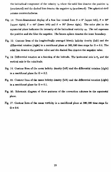
velocity ft. We adopt the frame of reference rotating with the angular velocity ft (see the left
panel of Fig. 1).
We normalize the variables by the following three parameters; the radius of the outer
spherical boundary, the density and the temperature at the outer boundary. Denoting the nor
malized time, mass density, pressure, temperature and velocity by t, pt p, T and v, respectively,
the governing normalized equations are written as follows:
| = - V - ( P V ) , (1)
gjipv) = - V • (pvv) - Vp + pg + 2pv x O + ji(VJv + | v ( V • v)), (2)
7 with
P = fiT,
«—fy r3
'2n(e««u-5(V-v)')
3
W
(5)
(6)
(7)
where 7(= 5/3), /( and A' are the adiabatic constant, normalized viscosity and normalized
thermal diffusivity, respectively, r is the position vector, </o is the gravity at the outer spherical
boundary (r = 1) and 0 is the dissipation function. e>3 is the stress tensor. The viscosity /* and
the thermal diffusivity K are assumed to be constant. We ignore the self-gravity of the fluid
and the centrifugal force. Using the equation of state (4), we can rewrite the thermodynamic^
equation (3) in the following way:
( ^ + v . V ) p = - 7 p V - v + ( 7 - l ) A - V 2 r + ( 7 - l ) $ . (8)
Note that the normalized sound velocity at the outer boundary is * /7« 1.29.
2.2 Initial and boundary conditions
The initial condition is given by the hydrostatic and thermal equilibrium state:
T(r) = l - / ? + £ , (9)
p(r) = T(r)m, (10)
v = 0, (II)
"" - 1 (12)
with
where $ > 0 is a constant and
is the polytropic index [20].
The temperatures at both the inner (hot) and outer (cold) spherical boundaries are fixed.
We adopt the stress-free boundary condition for the velocity.
2 .3 P h y s i c a l p a r a m e t e r s
The system has six independent parameters; r, ( the radius of the inner sphere), p
(normalized viscosity), K (normalized thermal diffusivity), g0 (gravity at the outer boundary),
ft (rotation rate of the ehell) and m (polytropic index). Other important non-dimensional
parameters which characterize the system are the Rayleigh number R, the Taylor number T
and the Prandtl number P which are given by
MK (13)
T-(2S£j", (14)
4
and p ~ ^ (»)
where d is the depth of the shell (d — 1 — r^). Note that the Rayleigh number of a stratified
fluid is a function of the depth [20], Here we measure the local Rayleigh number on the outer
spherical boundary (r = 1) because we normalize the variables by the values on this boundary.
The physical parameters used in this study are as follows. n = 0.5, p = 4 x 10~4,
A' = 1 x 10~3, gQ = 0.4 and m = 1. The local Rayleigh number and the Prandtl number for
these parameters are 3.52 x 10³ and 0.6. The remaining free parameter is the rotation rate of
the shell fi. We perform simulations for four different values of 0; 0 (without the rotation),
0.1, 0.2 and 0.4. We concentrate mainly on the results of ft = 0.4 in this paper. The Taylor
number is 2.50 x 10⁵ for this case.
The density stratification is a specific feature for a compressible fluid in the gravity field.
Note, however, that the density change in the spherical shell under the above parameters is
small: The density at the inner boundary is only 1.15.
2.4 Coordinate system and numerical method
We numerically solve the equations (1), (2) and (8) as an initial value problem on the
spherical coordinate system {r,9,<p), where r is the radius (0.5 < r < 1.0), 9 is the colatitude
(0 < 8 < 7r) and tp is the longitude (0 < <p < 2ir) (see the right panel of Fig. 1). The polar axis
6 = 0 is the direction of ft. We shall call the plane 9 — ir/2 as the equatorial plane.
We solve the above set of equations without any ad hoc assumptions, keeping the full
compressibility of the fluid. We, therefore, have the sound wave mode as well as the convection
mode. The maximum speed of the convection is about \% of the sound speed under the above
physical parameters.
We use the second-order finite difference in all (r, 9 and <p) directions. The total grid
number is 20 (radial) x46 (latitudinal) xl28 (longitudinal) for all the simulation runs. The
latitudinal grid spacing is A0 = 3.9* and the longitudinal grid spacing is &<p « 2.8*. Simulations
indicate that the convection velocity is organized as a set of many elongated columns aligned
to the rotation axis. Thus the finer grid mesh in the longitudinal direction than that in the
latitudinal direction is required.
We adopt the fourth-order Runge-Kutta-Gill (RKG) scheme for the time integration
[21, 22]. The length of the time step it determined by the Courant-Frtdrich-Levi condition:
a* =7.1 x lO"3.
5
There are two numerical difficulties to solve the finite difference equations on the spher
ical coordinate system. The difficulties and the numerical techniques developed to overcome
them are given in Appendix.
We begin the simulation run by adding a random temperature perturbation to the initial
equilibrium. Convective flows are excited by the perturbation since the initial condition is
unstable. We execute the time development of the convections for a sufficiently long time
(about 5.7 thermal diffusion time in the typical case).
3 Simulation Results
3.1 Formation of convection columns
The best way to reflect the effects of the rotation on the convection motion in the
spherical shell is to compare the saturated convection patterns of the two cases with and
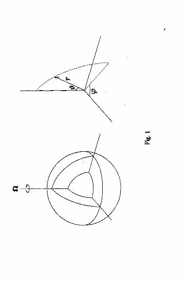
without the rotation. The two panels in Fig. 2 show the velocity field on a spherical cross
section of radius r = 0.75 (the middle of the spherical shell) for the case of ft = 0 (upper
panel) and for Q = 0.4 (lower panel). The contour line denotes the radial component of the
velocity. The solid line illustrates the rising (up-going) fluid region and the dashed line the
sinking (down-going) fluid region. All physical parameters in both cases are the same except
for the rotation rate. When the rotation is absent, the system is spherically symmetric so that
the convection cells have, of course, no preference for a particular direction. On the other hand,
when the shell is rotating, convection cells are elongated and alinged to the rotation axis [1].
We call them "convection columns" in this paper.
Although the initial temperature perturbation, which is imposed randomly, is not nec
essarily symmetric about the equator, Fig. 2 indicates that the saturated convection pattern is
symmetric about the equator [1].
Hereafter we wilt mainly investigate the convection for the case of Si = 0.4.
3.2 Temporal evolution of energy and helicity
In order to outline the evolution of the convection, we first show the time history of the
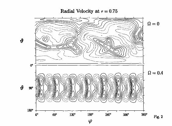
total volume integral of several quantities over the whole spherical shell. Fig. 3 shows the time
development of the volume integral of the kinetic energy (thick line), the differential rotation
kinetic energy (thin line) and the absolute value of the kinetic helicity density. (Because the
saturated convection motion is almost perfectly mirror symmetric about the equatorial plane,
6
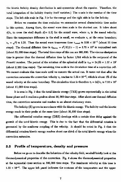
ihe kinetic helicity density distribution is anti-symmetric about the equator. Therefore, the
total integration of the helicity density itself vanishes.) The x-axis is the number of the time
steps. The left side scale in Fig. 3 is for the energy and the right side is for the helicity.
Before we examine the time evolution we summerize several characteristic time scales
in this system. Among them, the sound wave time scale is the shortest one. It takes about
dfvt to cross the shell depth d{= 0.5) for the sound wave, where v, is the sound velocity.
Since the temperature difference in the shell is small, we evaluate v, at the outer boundary;
vt = yft « 1.29. Then the sound wave transverse time rtound as 3.88 x 10 - 1 (about 55 time
steps). The thermal diffusion time is Ttherm = cP/K/d — 1) = 3.75 x 10² in normalized unit
(about 53,000 time steps). The total time steps of this run are 300,000. The viscous dissipation
time is greater than the thermal diffusion time by factor 1/0.6 which is the reciprocal of the
Prandtl number. The period of the rotation of the spherical shell is TTOt — 2ir/Q — 1.57 x 101
(about 2,200 time steps). The remaining time scale is the circulation time of a convection cell.
We cannot evaluate this time scale until we execute the actual run. It turns out that after the
convection saturates the convection velocity ve reaches to 1.33 x 10~2, which is about 1% of the
sound velocity at the outer boundary. The circulation time is therefore r, = 2d/vc « 7.52 x 101
(about 11,000 time steps).
It is seen in Fig. 3 that the total kinetic energy (TKE) grows exponentially in the initial
linear phase and it reaches a peak at about 30,000 time steps. After about one thermal diffusion
time, the convection saturates and reaches to an almost stationary state.
The helicity (H) grows in accordance with the kinetic energy. The helicity and the kinetic
energy reach to their peaks at the same time (about 30,000 time steps).
The differential rotation energy (DRE) develops with a certain time delay against the
growth of the total kinetic energy. This is due to the fact that the differential rotation is
generated by the nonlinear coupling of the velocity. It should be noted in Fig. 3 that the
differential rotation kinetic energy reaches about one third of the total kinetic energy when the
convection saturates.
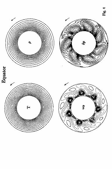
3.3 Profile of temperature, density and pressure
Before we go on to describe the behaviors of the velocity field, we shall briefly look at the
thermodynamic al properties of the convection. Fig. 4 shows the thermodynamical properties
at the equatorial cross section at 300,000 time steps. The maximum velocity at this time is
1.33 x 10**3. The upper left panel indicates the contours of the temperature and the upper
7
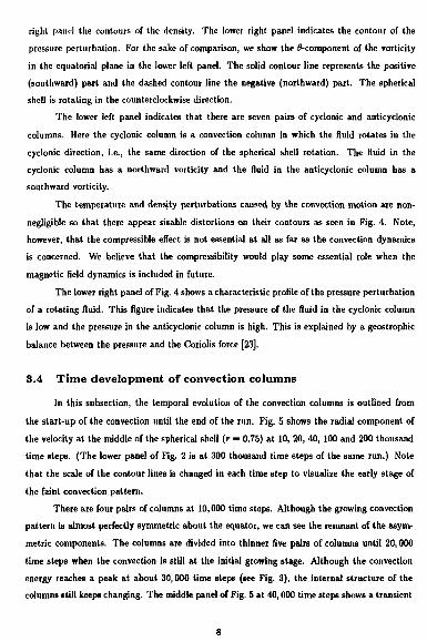
right panel the contours of the density. The lower right panel indicates the contour of the
pressure perturbation. For the sake of comparison, we show the ^-component of the vorticity
in the equatorial plane in the lower left panel. The solid contour line represents the positive
(southward) part and the dashed contour line the negative (northward) part. The spherical
shell is rotating in the counterclockwise direction.
The lower left panel indicates that there are seven pairs of cyclonic and anticyclonic
columns. Here the cyclonic column is a convection column in which the fluid rotates in the
cyclonic direction, i.e., the same direction of the spherical shell rotation. The fluid in the
cyclonic column has a northward vorticity and the fluid in the anticyclonic column has a
southward vorticity.
The temperature and density perturbations caused by the convection motion are non-
negligible so that there appear sizable distortions on their contours as seen in Pig. 4. Note,
however, that the compressible effect is not essential at all as far as the convection dynamics
is concerned. We believe that the compressibility would play some essential role when the
magnetic field dynamics is included in future.
The lower right panel of Fig. 4 shows a characteristic profile of the pressure perturbation
of a rotating fluid. This figure indicates that the pressure of the fluid in the cyclonic column
is low and the pressure in the anticyclonic column is high. This is explained by a geostrophic
balance between the pressure and the Coriolis force [23].
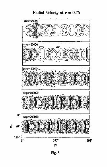
3.4 Time development of convection columns
In this subsection, the temporal evolution of the convection columns is outlined from
the start-up of the convection until the end of the run. Pig. 5 shows the radial component of
the velocity at the middle of the spherical shell (r = 0.75) at 10, 20, 40, 100 and 200 thousand
time steps. (The lower panel of Fig. 2 is at 300 thousand time steps of the same run.) Note
that the scale of the contour lines is changed in each time step to visualize the early stage of
the faint convection pattern.
There are four pairs of columns at 10,000 time steps. Although the growing convection
pattern is almost perfectly symmetric about the equator, we can see the remnant of the asym
metric components. The columns are divided into thinner five pairs of columns until 20,000
time steps when the convection is still at the initial growing stage. Although the convection
energy reaches a peak at about 30,000 time steps (see Fig. 3), the internal structure of the
columns still keeps changing. The middle panel of Fig. 5 at 40,000 time steps shows a transient
8
stage when the column pair number is decomposed into seven from the early four columns at
10,000 time steps. The cascade of the column decomposition ends at this mode number seven.
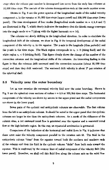
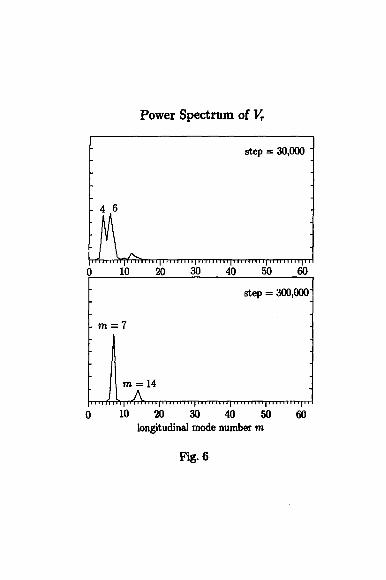
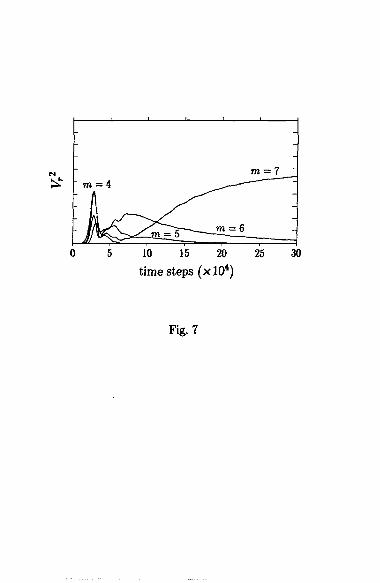
Shown in Fig. 6 are the power spectra of the longitudinal mode of the radial velocity
component vr in the equator at 30,000 time steps (upper panel) and 300,000 time steps (lower
panel). The time development of four modes (longitudinal mode number m = 4,5,6 and 7)
are illustrated in Fig. 7, which clearly indicates the tendency that the kinetic energy converges
into the single mode m = 7 (along with the higher harmonic m = 14).
The columns are slowly drifting in the longitudinal direction. In order to elucidate the
longitudinal drift of the columns, we show in Fig. 8 the temporal development of the radial
component of the velocity vT in the equator. The x-axis is the longitude (thus periodic) and
the y-axis is the time steps. The black region corresponds to vr > 0 (rising fluid) and the
white region vT < 0 (sinking fluid). This figure clearly shows the change of the number of the
convection columns and the longitudinal drifts of the columns. An interesting finding in this
figure is that the columns drift eastward until the convection saturates (about 30,000 time
steps) and then they drift westward. The westward drift velocity is about 2" per rotation of
the spherical shell.
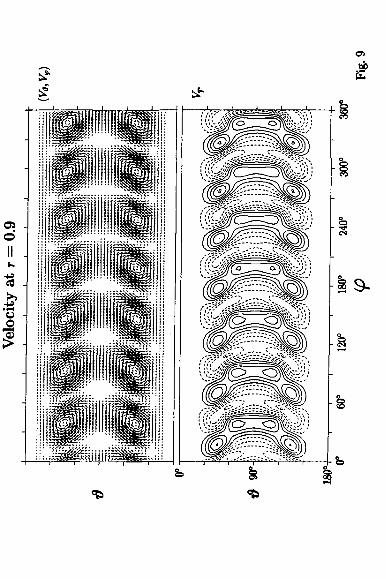
3.5 Velocity near the outer boundary
Let us now examine the saturated velocity field near the outer boundary. Shown in
Fig. 9 are the spherical cross sections of radius r = 0.9 at 300,000 time steps. The horizontal
components of the velocity are shown by arrows in the upper panel and the radial components
are shown in the lower panel.
Seven pairs of the cyclonic and anticyclonic columns are observable. The first column
from the left is an anticyclonic column. It should be noted in the upper panel that the cyclonic
columns are larger in size than the anticyclonic columns. As a result of the difference of the
column sizes, a net eastward zonal flow is generated near the equator and a westward zonal
flow at the high latitude region. In this way, an equatorial acceleration is generated-
Comparison of the behaviors of the horizontal and radial flows in Fig. 9 indicates that
there must exist the velocity component parallel to the rotation axis Q. The fluid in the
anticyclonic column "rises'1 from the equator toward both the northern and southern ends
of the column and then the fluid in the cyclonic column "sinks" from both ends toward the
equator. This is confirmed by the contour lines of radial component of the velocity field (the
lower panel). Hereafter, we shall call this fluid flow along the column axis as the axial flow
9
circulation in the direction of 11. The direction of the axial flow circulation indicates that
fluid parcels in both the cyclonic and anticyclonic columns experience the left-handed helical
trajectories in the northern hemisphere and the right-handed helical trajectories in the southern
hemisphere [24], The fluid, therefore, has a negative helicity in the northern hemisphere and a
positive helicity in the southern hemisphere.
Another lemakable feature observed in Fig. 9 is the crescent shape of the convection
patterns (see the lower panel). It is to be emphasized that the bending of the convection
pattern in the spherical cross section does not mean that the convection columns themselves
are bended. We will show in section 3.7 that the convection columns are certainly straight in
the direction of ft. The reason that despite the straight columns the contour lines exhibit the
bending structure will be explained in the next subsection.
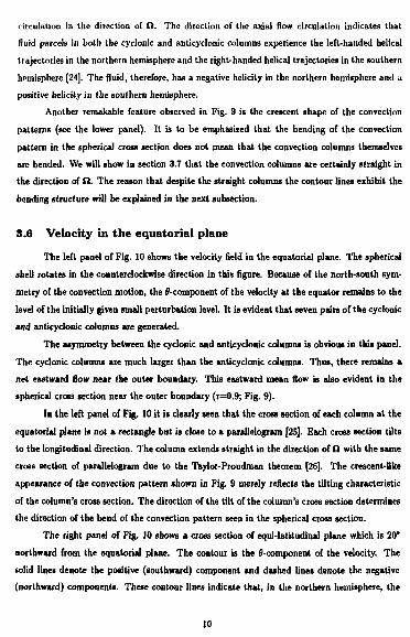
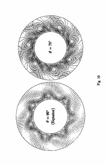
3.6 Velocity in the equatorial plane
The left panel of Fig. 10 shows the velocity field in the equatorial plane. The spherical
shell rotates in the counterclockwise direction in this figure. Because of the north-south sym
metry of the convection motion, the ^-component of the velocity at the equator remains to the
level of the initially given small perturbation level It is evident that seven pairs of the cyclonic
and anticycJonic columns are generated.
The asymmetry between the cyclonic and anticyclonic columns is obvious in this panel.
The cyclonic columns are much larger than the anticyclonic columns. Thus, there remains a
net eastward flow near the outer boundary. This eastward mean flow is also evident in the
spherical cross section near the outer boundary (r=0.9; Fig. 9).
In the left panel of Fig. 10 it is clearly seen that the cross section of each column at the
equatorial plane is not a rectangle but is close to a parallelogram [25]. Each cross section tilts
to the longitudinal direction. The column extends straight in the direction of ft with the same
cross section of parallelogram due to the Taylor-Proudman theorem [26]. The crescent-like
appearance of the convection pattern shown in Fig. 9 merely reflects the tilting characteristic
of the column's cross section. The direction of the tilt of the column's cross section determines
the direction of the bend of the convection pattern seen in the spherical cross section.
The right panel of Fig. 10 shows a cross section of equi-Jatitudina) plane which is 20'
northward from the equatorial plane. The contour is the ^-component of the velocity. The
solid lines denote the positive (southward) component and dashed lines denote the negative
(northward) components. These contour lines indicate that, in the northern hemisphere, the
10
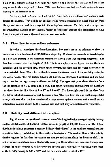
fluid in the cyclonic column flows from the northern end toward the equator and the other
way round in the anticyclonic column. This panel indicates us that the fluid circulates in each
column in the direction of (1.
In the cyclonic column, the fluid "sinks" from both the northern and southern ends
toward the equator. They collide at the equator and form a combined flow which wells out from
the cyclonic column and then merge into the anticyclonic column. The fluid, which merges into
an anticyclonic column at the equator, "rises" or "emerges" through the anticyclonic column
from the equator towards the northern and southern ends.
3.7 Flow Line in convection columns
In order to investigate the three-dimensional flow structure in the columns we show an
example of a flow line traced at 200,000 time steps. Fig. 11 shows the three-dimensional display
of a flow line (white) in the northern hemisphere viewed from four different directions. The
flow line is traced over the length of 12.5. The brown sphere in the figure denotes the inner
boundary and the greenish disk, which spans between, the inner and the outer boundaries, is
the equatorial plane. The color on the disk shows the ^-component of the vorticity cu§ in the
equatorial plane. The red region denotes the positive w» (southward vorticity) and the blue
region denotes the negative u/« (northward vorticity). The upper-left panel shows the view from
the the direction of 8 = 0, or from the north. The upper-right panel and the lower-left panel are
the views from the directions of 0 = 30* and 9 — 60". The lower-right panel is the view from
Q = 90' in which the equatorial disk becomes a line. The view from the due north (upper-left)
clearly indicates that the flow consists of a large vortex cyclonic column and a small vortex
anticyclonic column aligned to the rotation axis and that they are continuously connected,
3.8 Helicity and differential rotation
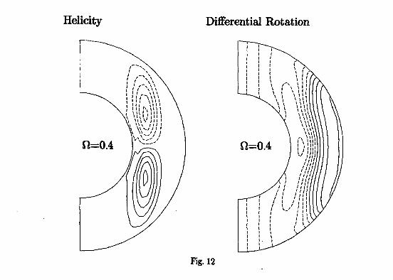
Fig. 12 shows the meridional cross sections of the longitudinally averaged helicity density
contours (left) and the differential rotation contours (right) at 300,000 time steps. The helical
flow in each column generates a negative helicity (dashed lines) in the northern hemisphere and
a positive helicity (solid lines) in the southern hemisphere. The contour lines of the helicity
density support the fact that the columns are straight and extend along the direction of O. The
anti-symmetrical distribution of the helicity density in the northern and southern hemispheres
reflects the mirror-symmetry of the convection motion about the equator. The maximum value
of the helicity density is 8.48 x 10~* and the minimum value is —8.48 x 10~*.
11
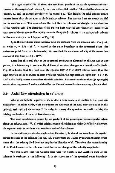
The right panel of Fig. 12 shows the meridional profile of the axially symmetrical com
ponent of the longitudinal velocity vv, i.e., the differential rotation. The solid line denotes the
positive vv and the dashed line denotes the negative vp. The fluid in the solid contour region
rotates faster than the rotation of the boundary spheres. The contour lines are nearly parallel
to the rotation axis. This also reflects the fact that the columns are straight in the direction
of the rotation axis. The distortion of the contour lines near the inner boundary indicates the
existence of the transverse flow which connects the cyclonic column to the anticyclonic column
in the west side (see the left panel of Fig. 10).
Vv in the meridional plane increases with the distance from the rotation axis. The peak,
at which vv = 2.95 x 10~3, is located at the outer boundary in the equatorial plane (the
outermost point from the rotation, axis.) We note that the maximum velocity of the convection
motion at this time is 1.33 x 10*"3.
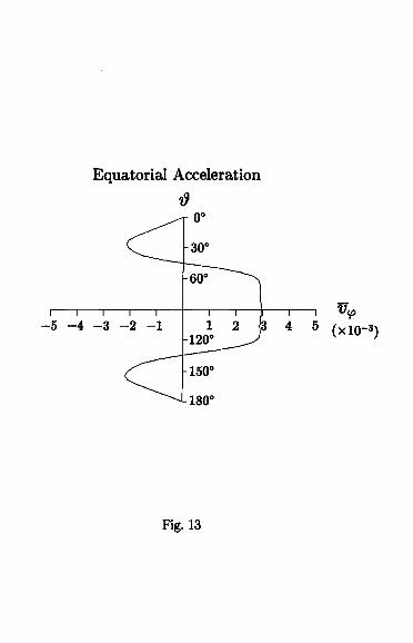
Regarding the zonal flow or the equatorial acceleration observed on the sun and major
planes, it is interesting to see how the differential rotation changes as a function of latitude.
Fig. 13 indicates that the fluid near the equator (60* < & < 120") rotates faster than the
rigid rotation of the boundary spheres while the fluid in the high latitude region ((0* < 9 < 45,
135* < 0 < 180*) rotates slower than the rigid rotation. This result confirms that the equatorial
acceleration is generated and maintained by the thermal convection in a rotating spherical shell.
3.9 Axial flow circulation in columns
Why is the helicity negative in the northern hemisphere and positive in the southern
hemisphere? In other words, what determines the diiection of the axial flow circulation in the
cyclonic and anticyclonic columns? In order to answer this question, we shall consider the
driving mechanism of the axial flow circulation.
The axial circulation is caused by the gradient of the geostrophic pressure perturbation
along the column axis, — V|p', which originates from the difference of the Coriolis force between
the equator and the northern and southern ends of the columns.
In the stationary state, the amplitude of the velocity is almost the same from the equator
toward the ends of the columns (see Fig. 12). This reflects the Taylor-Proudman theorem which
states that the velocity field does not vary in the direction of fl. Therefore, the nonuniformity
of the Coriolis force in the columns is not due to the change of the velocity amplitude.
The real reason that the Coriolis force near the northern and southern ends of the
columns is weakened is the following. It is the curvature of the spherical outer boundary.
12
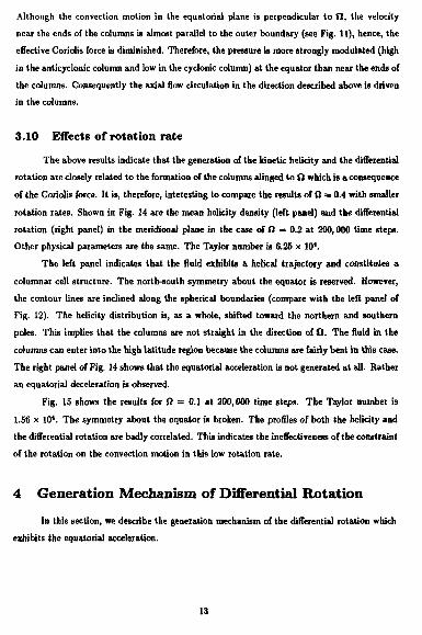
Although the convection motion in the equatorial plane is perpendicular to (2, the velocity
near the ends of the columns is almost parallel to the outer boundary (see Fig. 11), hence, the
effective Coriolis force is diminished. Therefore, the pressure is more strongly modulated (high
in the anticyclonic column and low in the cyclonic column) at the equator than near the ends of
the columns. Consequently the axial flow circulation in the direction described above is driven
in the columns.
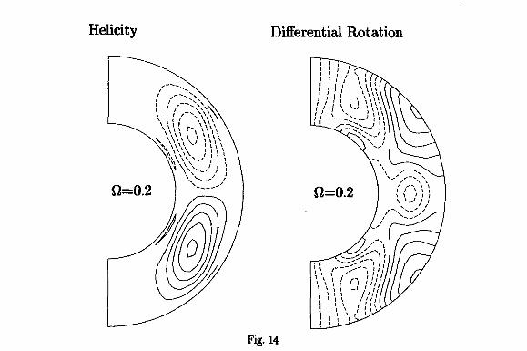
3.10 Effects of rotation rate
The above results indicate that the generation of the kinetic helicity and the differential
rotation are closely related to the formation of the columns alinged to fl which is a consequence
of the Coriolis force. It is, therefore, interesting to compare the results of ft = 0.4 with smaller
rotation rates. Shown in Fig. 14 are the mean helicity density (left panel) and the differential
rotation (right panel) in the meridional plane in the case of ft = 0.2 at 200,000 time steps.
Other physical parameters are the same. The Taylor number is 6.25 x 10*.
The left panel indicates that the fluid exhibits a helical trajectory and constitutes a
columnar cell structure. The north-south symmetry about the equator is reserved. However,
the contouT lines are inclined along the spherical boundaries (compare with the left panel of
Fig. 12). The helicity distribution is, as a whole, shifted toward the northern and southern
poles. This implies that the columns are not straight in the direction of fl. The fluid in the
columns can enter into the high latitude region because the columns are fairly bent in this case.
The right panel of Fig. 14 shows that the equatorial acceleration is not generated at all. Rather
an equatorial deceleration is observed.
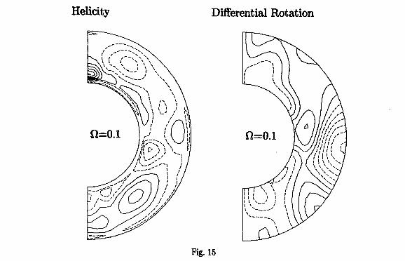
Fig. 15 shows the results for Q = 0.1 at 200,000 time steps. The Taylor number is
1.56 x 10*. The symmetry about the equator is broken. The profiles of both the helicity and
the differential rotation are badly correlated. This indicates the ineffectiveness of the constraint
of the rotation on the convection motion in this low rotation rate.
4 Generation Mechanism of Differential Rotation
In this section, we describe the generation mechanism of the differential rotation which
exhibits the equatorial acceleration.
13
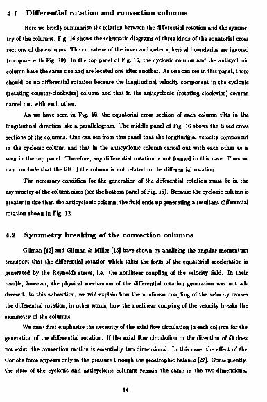
4 .1 D i f f e r en t i a l r o t a t i o n a n d c o n v e c t i o n c o l u m n s
Here we briefly summarize the relation between the differential rotation and the symme
try of the columns. Fig. 16 shows the schematic diagrams of three kinds of the equatorial cross
sections of the columns. The curvature of the inner and outer spherical boundaries are ignored
(compare with Fig. 10). In the top panel of Fig. 16, the cyclonic column and the anticyclonic
column have the same size and are located one after another. As one can see in this panel, there
should be no differential rotation because the longitudinal velocity component in the cyclonic
(rotating counter-clockwise) column and that in the anticyclonic (rotating clockwise) column
cancel out with each other.
As we have seen in Fig. 10, the equatorial cross section of each column tilts in the
longitudinal direction like a parallelogram. The middle panel of Fig. 16 shows the tilted cross
sections of the columns. One can see from this panel that the longitudinal velocity component
in the cyclonic column and that in the anticyclonic column cancel out with each other as is
seen in the top panel. Therefore, any differential rotation is not formed in this case. Thus we
c*n conclude that the tilt of the column is not related to the differential rotation.
The necessary condition for the generation of the differential rotation must lie in the
asymmetry of the column sizes (see the bottom panel of Fig. 16). Because the cyclonic column is
greater in size than the anticyclonic column, the fluid ends up generating a resultant differential
rotation shown in Fig. 12.
4.2 Symmetry breaking of the convection columns
Gilman [12] and Gilman & Miller [15] have shown by analizing the angular momentum
transport that the differential rotation which takes the form of the equatorial acceleration is
generated by the Reynolds stress, i.e., the nonlinear coupling of the velocity field. In their
results, however, the physical mechanism of the differential rotation generation was not ad
dressed. In this subsection, we will explun how the nonlinear coupling of the velocity causes
the differential rotation, in other words, how the nonlinear coupling of the velocity breaks the
symmetry of the columns.
We must first emphasize the necessity of the axial flow circulation in each column for the
generation of the differential rotation. If the axial flow circulation in the direction of ft does
not exist, the convection motion is essentially two dimensional. In this case, the effect of the
Goriolis force appears only in the pressure through the geostrophic balance [27]. Consequently,
the sizes of the cyclonic and anticyclonic columns remain the same in the two-dimensional
14
flow. Therefore, the axial flow circulation is concluded to be essential for the generation of the
differential rotation.
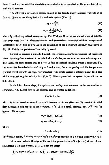
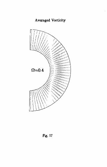
The differential rotation is closely related to the longitudinally averaged vorticity w as
follows. (Here we use the cylindrical coordinate system (R,<f>,z).)
*>—%< ( , 6 )
* • - * & * * > • ( I 7 )
where v+ is the longitudinal average of vv. Fig. 17 shows W in the meridional plane at 300,000
time steps when fi = 0.4. The formation of the differential rotation which exhibits the equatorial
acceleration (Fig. 12) is equivalent to the generation of the northward vorticity flux shown in
Fig. 17. This is the problem of "vorticity dynamo".
Here let us consider a simplified model. We concentrate on the region near the equatorial
plane. Ignoring the curvature of the spherical boundaries, we use a cartesian coordinate system.
The equatorial plane corresponds to z = 0. A fluid is confined in a layer which is surrounded by
the stress-free boundaries located at y = 0 and y — IT. Both the gravity and the temperature
gradient direct towards the negative y direction. The whole system is rotating about the z-axis
with a constant angular velocity II = (0,0,0). We suppose that the system is periodic in the
x-direction.
In the initial linear stage, the cyclonic and anticyclonic columns can be assumed to be
symmetric. The helical flow in the columns can be written as follows.
v » v 0 + fV|, (18)
where Vo is the two-dimensional convective motion in the x-y plane and Vi denotes the axial
flow circulation component in the columns, e (> 0) is a small constant and Ofe3) will be
ignored. We suppose
Vi = < - M , 0 , - * f l , (20)
where
t/< = sinisiny. (21)
The helicity density h = v*w = —2cz(sin2a:+sinJy) is negative in z > 0 and positive in z < 0.
Let us now evaluate the sign of the vorticity generation rate V x (v x w) at the column
boundaries x = 0 and ir where ut = 0. Then we obtain
JJ[v x (v x «)],<*„ = e^vxwj^y-Kv *«),];:;
15
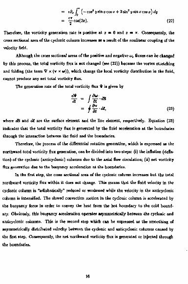
= tds I (— cos2 y sin x cos x + 2 sin2 y sin x cos a 1 dy
= yC M (2x) . (22)
Therefore, the vorticity generation rate is positive at x = 0 and z = r. Consequently, the
cross sectional area of the cyclonic column increases as a result of the nonlinear coupling of the
velocity field.
Although the cross sectional areas of the positive and negative wt fluxes can be changed
by this process, the total vorticity flux is not changed (see (22)) because the vortex stretching
and folding (the term V x (v x w)), which change the local vorticity distribution in the fluid,
cannot produce any net total vorticity flux.
The generation rate of the total vorticity flux $ is given by
dt ~ J dt dS dv
/ * • * w» where dS and dl are the surface element and the line element, respectively. Equation (23)
indicates that the total vorticity flux is generated by the fluid acceleration at the boundaries
through the interaction between the fluid and the boundaries.
Therefore, the process of the differential rotation generation, which is expressed as the
northward total vortictty flux generation, can be divided into two steps: (i) the inflation (defla
tion) of the cyclonic (anticyclonic) columns due to the axial flow circulation; (ii) net vorticity
flux generation due to the buoyancy acceleration at the boundaries.
In the first step, the cross sectional area of the cyclonic column increases but the total
northward vorticity flux within it does not change. This means that the fluid velocity in the
cyclonic column is "adiabatically" reduced or weakened while the velocity in the anticyclonic
column is intensified. The slowed convection motion in the cyclonic column is accelerated by
the buoyancy force in order to convey the heat from the hot boundary to the cold bound
ary. Obviously, this buoyancy acceleration operates asymmetrically between the cyclonic and
anticyclonic columns. This is the second step which can be expressed as the smoothing of
asymmetrically distributed velocity between the cyclonic and anticyclonic columns caused by
the first step. Consequently, the net northward vorticity flux is generated or injected through
the boundaries.
16
5 Summary
In a rotating spherical shell convection, the velocity is organized as a set of convection
columns alinged to the rotation axis ft because of the constraint of the Coiiolis force. If the
rotation is sufficiently rapid, the columns extend straight in the direction of O. This configura
tion inevitably causes the axial flow circulation along the column axis. The combination of the
axial flow circulation and the rotating convective motion produces a negative kinetic heticity
in the northern hemisphere and positive helicity in the southern hemisphere.
The differential rotation which takes the form of equatorial acceleration is expressed as
the mean northward vorticity flux. The generation of the differential rotation can, therefore,
be rephrased as a vorticity dynamo problem.
The cyclonic column has a northward vorticity flux and the anticydonic column has a
southward vortidty flux. Therefore, the spherical shell is filled with pairs of the vortidty fluxes
with opposite polarities. If the cyclonic column and the anticyclonic column are perfectly
symmetric, the total vorticity flux is zero since both fluxes cancel out with each other. The
equatorial acceleration is a consequence of the fact that the northward vortidty flux in the
cyclonic column glows more effectively than the southward vorticity flux in the anticydonic
column.
The axial flow circulation in each column inflates the cyclonic columns and deflates the
anticyclonic columns due to the nonlinear coupling of the velodty field. The vortidty flux,
however, cannot be generated by this process because it is merely a vortex stretching and fold
ing. The inflation of the cyclonic column reduces the velodty in the cyclonic column while the
velocity in the anticyclonic column is intensified. The asymmetric velocity distribution in the
columns is smoothed by the buoyancy acceleration at the boundaries. In order to compensate
the rarefied northward vorticity flux in the cyclonic columns, the northward vorticity flux must
be injected through the boundaries. Thus a net northward vorticity flux is generated as a result
of the nonlinear coupling of the convection columns.
The results obtained in this study indicate that the convection motion in a rapidly
rotating spherical shell generates a differential rotation where an equatorial acceleration takes
place by the selective growth of the cyclonic convection columns.
Acknowledgements
The authors are grateful to Professor K. Nishikawa for his encouragement through out
ir
this work. The authors arc also grateful to Professor R. Horiuchi and Dr. K. Kusano for valuable
discussions. This research is supported by a Giant-in-Aid from the Ministry of Education,
Science and Culture in Japan.
18
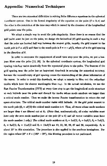
Appendix: Numerical Techniques
There are two numerical difficulties in solving finite difference equations in the spherical
coordinate system. One is the formal singularity of the equation on the poles (0 — 0, TT) and
the other is the restriction of the time step which is caused by the closeness of the longitudinal
grid points near the poles.
We adopt a simple way to avoid the pole singularity. Since there is no reason that the
grid point must be just on the poles, we design the latitudinal (0) grid spacing in such a way
that the poles are located half way between the nearest grids, namely, the grid nearest to the
north pole is 9 = &B/2 and that to the south pole is 9 = T — A0/2, where A0 is the grid spacing
in the direction of 9.
In order to overcome the requirement of small time step near the poles, we put a low-
pass filter near the poles [12, 28]. In the spherical coordinate system, the longitudinal grid
spacing r$in0&<p varies drastically from the equatorial plane to the poles. The fineness of the
grid spacing near the poles has an important drawback in securing the numerical accuracy,
because the nonuniformity of grid spacing causes the mismatching of the phase information of
the waves. In order to avoid this drawback, we adopt a remedy to filter out the redundant
modes which have the shorter wavelengths than r&p. In the actual calculation, we use the
Fast Fourier Transformation (FFT) at every time step to get the longitudinal mode structure
at each latitude near the poles and discard the modes whose mode numbers are larger than
a critical mode number. Then we make the inverse Fourier transformation to return the real
space structure. The critical mode number varies with latitude. At the grid point nearest to
the north pole ($i = &&/2) the critical mode number is 4. Thus, all waves whose mode numbers
are larger than 4 are filtered out at $\. (Note that, mathematically, all scalar variables must
have only the zero mode number just at the pole (9 = 0) and all vector variables must have
the mode number 1 only.) The critical mode numbers at 82 = 3A0/2, 9$ - 5&0/2, 9A ~ 7*9/2,
05 = 9*9/2, Ba = 11&0/2 and 67 = 13*0/2 are 13, 22, 30, 39, 47 and 56, respectively. 97 is
about 25" in this simulation. The procedure is also applied to the southern hemisphere. For
the region where 25" < 9 < (180" - 25*), this filtering procedure is not performed.
19
References
[1] F. H. Busse. J. Fluid Mech., 44, 441, 1970.
[2] F. H. Busse. Aatrophya. J., 159, 629, 1970.
[3] F. H. Busse. Astron. k Astrophys., 28, 27, 1973.
[4] F. H. Busse and C. R. Carrigan. J. Fluid Mech., 62, 579, 1974.
[5] F. H. Busse and C. R. Cairigan. Science, 191, 81, 1976.
[6] F. H. Busse and P. G. Cuong. Geophya. Aatropkys. Fluid Dyn., 8, 17, 1977.
[7] C. R. Carrigan and F. H. Busse. J. Fluid Mech., 126, 287, 1983.
[8] J. A. Chamberlain and C. R. Carrigan. Geophya. Aalrophya. Fluid Dyn., 35, 303, 1986.
[9] G. A. Glatzmaier J. E. Hart and J. Toomrc. J. Fluid Mech., 173, 519, 1986.
[10] S. Cordero and F. H. Busse. Geophya. Rea. Lett., 19, 733, 1992.
[11] P. A. Gilroan. J. Aimoaph. Science, 32, 1331, 1975.
[12] P. A. Gilman. Geophys. Astropkya. Fluid Dyn., 8, 93, 1977.
[13] P. A. Gilman. Geophya. Aalrophya. Fluid Dyn., 11, 157, 1978.
[14] P. A. Gilman. Geophya. Aatrophya. Fluid Dyn., 11, 181, 1978.
[15] P. A. Gilman and 3. Miller. Aatrophya. J. Suppl, 61, 585, 1986.
[16] K. Zhang and F. H. Busse. Geophys. Aatrophya. Fluid Dyn., 39, 119, 1987.
[17] K. Zhang. Geophys. Res. Lett, 18, 685, 1991.
[18] K. Zhang. J. Fluid Mech., 236, 535, 1992.
[19] P. A. Gilman and G. A. Glatzmaier. Astrophys. J. Suppl., 45, 335, 1981.
[20] E. A. Spiegel. Astrophys. J., 141, 1068,1964.
[21] R. Horiuchi and T. Sato. Phya. Fluid, Bl , 581, 1989.
[22] K. Watanabe and T. Sato. J. Geophys. Res., 95, 1990.
20
[23] A. S. Monin. Theoretical geophysical fluid dynamics. Kluwet Academic Publishers, 1988.
[24] P. A. Gilman. Astropkys. J. Suppl., 53, 243, 1983.
[25] F. H. Busse and A. C. Ot. Geophys. Astrophys. Fluid Dyn., 21, 59, 1986.
[26] S. Chandrasekhat. Hydrodynamic and Hydromagnetic Stability. Dover, 1968.
[27] F. H. Busse and L. L. Hood. Geopkys. Astropkys. Fluid Dyn., 21, 59, 1982.
[28] M. J. P. Cullen. J. Comp. Phys., 50, 1, 1983.
21
Figure Captions
Fig. I: Geometry of the convection vessel (left panel) and the spherical coordinate system r
(radius), 6 (colatitude) and <p (longitude).
Fig. 2: Contour lines of the radial component of the velocity at the middle of the spherical
shell (r = 0.75) for the case of ft = 0 (upper panel) and Q = 0,4 (lower panel). The solid
line denotes the rising fluid and the dashed line denotes the sinking fluid.
Fig. 3: Time development of the total energy (solid thick line), the differential rotation kinetic
energy (thin Une) and the helicity (dashed line) for the case of 12 = 0.4. The left side
scale is for the energy and the right side scale is for the helicity.
Fig. 4: Contour lines of the temperature (upper left panel), density (upper right), latitudinal
component of the vorticity (lower left) and the pressure perturbation (lower right panel)
in the equatorial plane. The solid contour denotes the positive value and the dashed
contour denotes the negative value. The spherical shell rotates in the counterclockwise
direction in this figure.
Fig. 5: Time development of the convection pattern in the middle of the spherical shell (r =
0.75).
Fig. 6: Power spectra of the longitudinal mode of the radial component velocity vr at the
equator at 30,000 time steps (upper panel) and 300,000 time steps (lower panel).
Fig. 7: Time development of the longitudinal modes of the radial component velocity vr at
the equator.
Fig. 8: Time development of the convection columns. The black (white) regions correspond to
the regions where the fluid rises (sinks) at the middle of the shell in the equatorial plane
(r = 0.75).
Fig. 9: Flow distributions of the horizontal component (upper panel) and the radial component
(lower panel) of the velocity on a spherical surface near the outer boundary (r = 0.9) at
300,000 time steps. The solid line denotes the rising part of the fluid and the dashed line
denotes the sinking part.
Fig. 10: Flow distributions of the velocity vectors in the equatorial plane (0 = 90*) and in the plane (0 = 70') at 300,000 time steps. The contour line on the right shows
22
the latitudinal component of the velocity vg where the solid line denotes the positive vg
(southward) and the dashed line denotes the negative vg (northward). The spherical shell
rotates counterclockwise.
Fig. 11: Three-dimensional display of a flow line viewed from 5 = 0 ° (upper left), $ = 30"
(upper right), B = 60° (lower left) and 8 = 90* (lower right). The color plot in the
equatorial plane indicates the intensity of the latitudinal vorticity w». The red expresses
the positive and the blue the negative. The brown sphere denotes the inner boundary.
Fig. 12: Contour lines of the longitudinally averaged kinetic helicity density (left) and the
differential rotation (right) in a meridional plane at 300,000 time steps for ft = 0.4. The
solid line denotes the positive value and the dashed line denotes the negative value.
Fig. 13: Differential rotation as a function of the latitude. The horizontal axis is vv and the
vertical axis is the colatitude.
Fig. 14: Contour lines of the mean helicity density (left) and the differential rotation (right)
in a meridional plane for Q = 0.2.
Fig. 15: Contour lines of the mean helicity density (left) and the differential rotation (right)
in a meridional plane for ft = 0.1.
Fig. 16: Schematic diagram of three patterns of the convection columns in the equatorial
plane.
Fig. 17: Contour lines of the mean vorticity in a meridional plane at 300,000 time steps for
ft = 0.4.
23
Radial Velocity at r = 0.75
#
$ 90°
180° 0° 60° 120°
i i 1 1 1 r-180° 240° 300°
n = o
¥>
fi = 0.4
360° Fig. 2
time steps (xlO4)
Fig. 3
Radial Velocty at r = 0.75
step=40000....,
Fig. 5
Power Spectrum of VT
step = 30,000
• 4 6
•Wftftr i iTjrnITT11111111 n 111 f rn 111'n i |-i 11 n 1111| 111111111111 0 10 20 30 40 50 60
step = 300,000
m = 7
m = 14
rA 11 n | m i n 111 rm 111111 (111111111 p 1111111 IJ 111111 n 1111 0 10 20 30 40 50 60
longitudina] mode number m
Fig. 6
10 15 20
time steps (xlO4) 25 30
Fig. 7
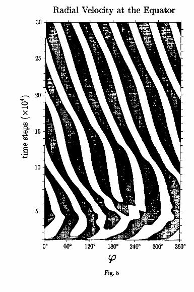
Radial Velocity at the Equator
120° 180° 240° 300° 360°
Fig. 8
60
OS ©
18 >>
•+3
o
o
S9-
I?
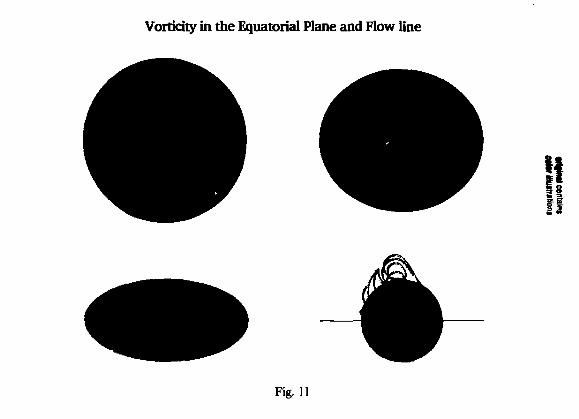
Vorticfty in the Equatorial Plane and Flow line
H i
Fig. 11
Helicity Differential Rotation
Fig. 12
Equatorial Acceleration
Fig. 13
Helicity Differential Rotation
Fig. 14
Helicity Differential Rotation
ft=0.1
Fig. 15
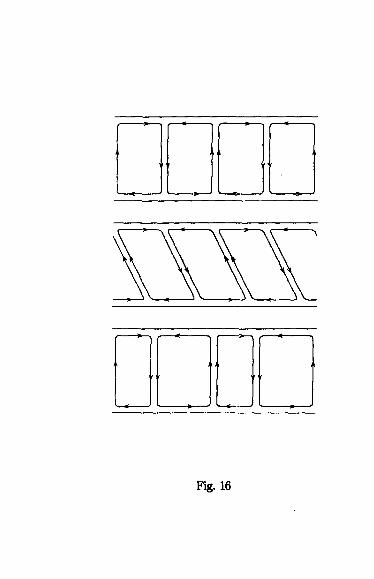
Fig. 16
Averaged Vorticity
Fig. 17
Recent Issues of NIFS Series
NIFS-165 T. Sekl, R. Kumazawa, T. Watari, M. Ono, Y. Yasaka, F. Shimpo, A. Ando, O. Kanaka, Y. Oka, K. Adatl, R. Aklyama, Y. Hamada, S. Hktekuma, S. Hlrokura, K. Ida, A. Karita, K. Kawahala, Y. Kawasumi, Y. Kitoti, T. Kohmoto, M. Kojima, K. Maaai, S. Morita, K. Narihara, Y. Ogawa, K. Ohkubo, S. Okajima, T. Ozakl, M. Sakamoto, M. Sasao, K. Sato, K. N. Sato, H. Takahaahi, Y. TaniflucW, K. Toi and T. Tsuzuki, High Frequency Ion Bernstein Wave Heating Experiment on JIPP T-IIU Tokamak; Aug. 1992
NIFS-166 Vo Hong Anh and Nguyen Tien Dung, A Synergetic Treatment of the Vortices Behaviour of a Plasma with Viscosity; Sep. 1992
NIFS-167 K.Watanabe and T.Sato, A Triggering Mechanism of Fast Crash in Sawtooth Oscillation; Sep. 1992
NIFS-168 T. Hayashi, T. Sato, W. Lotz, P. Merkel, J. NQhrenberg, U. Schwann and E. Strumberger, 3D MHD Study of Helios and Heliotron; Sap. 1992
NIFS-169 N. Nakajkna, K. Ichlguchi, K. Watanabe, H. Sugama, M. Okamoto, M. Wakatani, Y. Nakamura and C. Z. Cheng, Neoclassical Current and Related MHD Stability, Gap Modes, and Radial Electric Field Effects in Heliotron and Torsatron Plasmas: Sep. 1992
NIFS-170 H. Sugama, M.Okamoto and M. Wakatani, K-c Model of Anomalous Transport in Resistive Interchange Turbulence; Sap, 1992
NIFS-171 H. Sugama, M. Okamoto and M. Wakatani, Vlasov Equation in the Stochastic Magnetic Field ; Sep. 1992
NIFS-172 N. Nakajima, M. Okamoto and M. Fujiwara, Physical Mechanism of E . -Driven Current in Asymmetric Toroidal Systems; Sep.1992
NIFS-173 N. Nakajima, J. Todoroki and M. Okamoto, On Relation between Hamada and Boozer Magnetic Coordinate System; Sep. 1992
NIFS-174 K. Ichiguchi, N. Makajlma, M. Okamoto, Y. Nakamura and M. Wakatani, Effects of Net Toroidal Current on Mercier Criterion in the Large Helical Device ; Sap. 1992
NIFS-175 S. -I. Hon, K. Hon and A. Fukuyama, Modelling ofELMs and Dynamic Responses of the H-Mode; Sep. 1992
NIFS-176 K. Itoh, S.-l. Iloh, A. Fukuyama, H. Sanukl, K. Ichlguchi and J. Todoroki, Improved Models of p-Limit, Anomalous Transport
and Radial Electric Field with Loss Cone Loss in Heliotron I Torsatron ; Sep. 1992
NIFS-177 N. Ohyabu, K. Yamazaki, I. Katanuma, H. Ji, T. Watanaba, K. Watanabe. H. Akao, K. Akaishi, T. Ono, H. Kaneko, T. Kawamura, Y. Kubota. N. Noda, A. Sagara, O. Motojime, M. Fujiwara and A. liyoshl, Design Study of WD Helical Divertor and High Temperature Divertor Plasma Operation; Sep. 1992
NIFS-178 H. Sanukl, K. Itoh and S.-l. Itoh, Selfconsistent Analysis of Radial Electric Field and Fast Ion Losses in CHS Torsatron I Heliotron ; Sep. 1992
NIFS-179 K. Toi. S. Morita, K. Kawahata, K. Ida, T. Watari, R. Kumazawa, A. Ando, Y. Oka, K. Ohkubo, Y. Hamada, K. AdaU, R. Akiyama, S. Hidekuma, S. Hlrokura, 0. Kaneko, T. Kawamoto, Y. Kawasuml, M. Kojima. T. Kuroda, K. Masai, K. Narihara, Y. Ogawa, S. Okajima, M. Sakamoto, M. Sasao. K. Sato. K. N. Sato, T. Seki, F. Shimpo, S. Tanahashi, Y. Taniguchi, T. Tsuzuki, New Features ofL-H Transition in Limiter H-Modes ofJIPP T-HU; Sep. 1992
H. Momota, Y. Tomita. A. Ishkta, Y. Kohzakl, M. Ohnishi, S. Ohl,
Y. Nakao and M. Nishlkawa. D-3He Fueled FRC Reactor "Artemis-L" ; Sep. 1992 T. Watari, R. Kumazawa, T. Seki, Y. Yasaka, A. Ando, Y. Oka.O. Kaneko, K. Adatl, R. Akiyama, Y. Hamada, S. Hidekuma. S. Hlrokura, K. Ida, K. Kawahata, T. Kawamoto, Y. Kawasuml, S. Kitagawa, M. Kojima, T. Kuroda, K. Masai, S. Morita, K. Narihara, Y. Ogawa, K. Ohkubo, S. Okajima, T. Ozakl, M. Sakamoto, M. Sasao, K. Sato, K. N. Sato, F.Shlmpo, H. Takahashi, S. Tanahasi, Y. Taniguchi, K. Toi, T. Tsuzuki and M. Ono, The New Features of Ion Bernstein Wave Heating in JIPP TIIU Tokamak ,Sep, 1992
NIFS-182 K. Itoh, H. Sanukl and S.-l. Itoh, Effect of Alpha Particles on Radial Electric Field Structure in Torsatron I Heliotron Reactor, Sap. 1992
NIFS-183 S. Morimoto, M. Sato, H. Yamada, H. Ji, S. Okamura, S. Kubo, O. Motojima, M. Murakami, T. C. Jemigan, T. S. Bigatow, A. C. England, R. S. Isler, J. F. Lyon, C. H. Ma, D. A. Rasmussen, C. R. Sohaksh, J. B. WHgen and J. L. Yarber, Long Pulse Discharges Sustained by Second Harmonic Electron Cyclotron Heating Using a 35GHZ Gyrotron in the Advanced Toroidal Facility; Sap. 1992
NIFS-184 S. Okamura, K. Hanatanl, K. Nithimura, R. Akiyama, T. Amano, H. Arknoto, M. Fujiwara, M. Hosokawa, K. Ida. H. Idal, H. Iguchi, O. Kaneko, T. Kawamoto, S. Kubo, R. Kumazawa, K. Malauoka, S. Morita, O. Molojima, T. Mutoh, N. Nakajima, N. Noda, M. Okamolo, T. Ozakl, A. Sagara, S. Sakakibara, H. Sanuki, T. Seki. T. ShoJI,
NIFS-180
NIFS-181
F. Sbimbo, C. Takahaahi, Y. Takeki, Y. TakHa, K. Toi, K. Taumofi. M. Ueda, T. Watarl, H. Yamada and I. Yamede, Heating Experiments Using Neutral Beams with Variable Injection Angle and ICKF Waves in CHS; Sep. 1992
NIFS-185 H. Yamada, S. Morita, K. Ida, S. Okamun, H. kjuchi, S. SaKaWbara, K. Nishimura, R. Akiyama, H. Arimolo, M. Fujiwara, K. Hanatanl, S. P. Hlrshman, K. tefifguchi, H. fctol, O. Kantko, T. Kawamoto, S. Kubo, D. K. Lee, K. Matsuoka, O, Motojima, T. Ozakl, V. D. Pustovitov, A. Sagara, H. Sanukl, T. Shoji, C. Takahaahi, Y. Takeiri, Y. Taklta, S. Tanahashl, J. Todorokl, K. Tol, K. Taumori, M Ueda and I. Yamada, MHD and Confinement Characteristics in the High-fi Regime on the CHS Low-Aspect-Ratio Heliotrm I Torsatron : Sep. 1992
NIFS-186 S. Morita. H. Yamada, H. Iguchl, K. Adatl, R. AJdyama, H. Arimolo, M. Fujiwara, Y. Hamada, K. Ida, H. Idei, O. Kaneko. K. Kawahata, T. Kawamoto, S. Kubo, R. Kumazawa, K. Matsuoka, T. Mdrisaki, K. Nishimura, S. Okamura, T. Ozaki. T. Seki, M. Sakurai, S, Sakakibara, A. Sagara, C. Takahashi, Y. Takeiri, H. Takenaga, Y. Takita, K. Toi, K. Tsumori, K. Uchino, M. Ueda, T. Watarl, I. Yamada, A Role of Neutral Hydrogen in CHS Plasmas with Reheat and Collapse and Comparison with JIPP T-ttU Tokamak Plasmas ; Sep. 1992
NIFS-187 K. loth. S.-l. Itoh, A. Fukuyama, M. Yagi and M. Azumi. Model of the L-Mode Confinement in Tokamaks; Sep. 1992
NIFS-188 K. Itoh, A. Fukuyama and S.-l. Itoh, Beta-Limiting Phenomena in High-Aspect-Ratio Toroidal Helical Plasmas; Oct. 1992
NIFS-189 K. Itoh, S. -I. Itoh and A. Fukuyama, Cross Field Ion Motion at Sawtooth Crash ; Oct. 1992
NIFS-190 N. Noda. Y. Kubota, A. Sagara, N. Ohyabu, K. Akaiahl, H. Ji, O. Motojima, M. Hashlba, I. Fujita, T. Hino, T. Yamashlna, T. Matsuda, T. Sogabe. T. Matsumoto, K. Kuroda, S. Yamazakl, H. Ise, J. Adachi and T. Suzuki, Design Study on Divertor Plates of Large Helical Device (LHD); Oct. 1992
NIFS-191 Y. Kondoti, Y. Hosaka and K. IshH, Kernel Optimum Nearly-Analytical Discretization (KOND) Algorithm Applied to Parabolic and Hyperbolic Equations : Oct. 1892
NIFS-192 K. Itoh, M. Yagi, S.-l. Itoh, A. Fukuyama and M. Azumi, L-Mode Confinement Model Based on Transport-MHD Theory in Tokamaks ; Oct. 1992
NIFS-193 T. Watari, Review of Japanese Results on Heating and Current
Drive; Oct. 1992
NIFS-194 Y. Kondoh, Eigenfunction for Dissipative Dynamics Operator and Attractor of Dissipative Structure; Oct. 1992
NIFS-195 T. Wannabe, H. Oya, K. Watanaba and T. Salo, Comprehensive Simulation Study on Local and Global Development of Auroral Arcs and Field-Aligned Potentials ; Oct. 1992
NIFS-196 T. Mori, K. Akalshi, Y. Kubota, O. Molojima, M. Muahiaki, Y. Funato and Y. Hanaoka, Pumping Experiment of Water on B and LaB6 Films with Electron Beam Evaporator; Oct., 1992
NIFS-197 T. Kato and K. Maul, X-ray Spectra from Hinotori Satellite and Suprathermal Electrons; Oct. 1992
NIFS-198 K. Toi, S. Okamura, H. Igucril, H. Yamada, S. Morita, S. Sakakibara, K. Ida, K. Minimum, K. Matsuoka, R. Akryama, H. Arlmoto, M. Fujhvara, M. Hotokawa, H. ktei, O. Kaneko, S. Kubo, A. Sagara, C. Takahashl, Y. Takalri, Y. Taklta, K. Tsumori, I. Yamada and H. Zushi, Formation of H-mode Like Transport Barrier in the CHS Heliotron I Torsatron; Oct 1992
NIFS-199 M. Tanaka, A Kinetic Simulation of Low-Frequency Electromagnetic Phenomena in Inhomogeneous Plasmas of Three-Dimensions ; Nov. 1992
NIFS-200 K. Itoh, S.-l. Itoh, H. Sanukl and A. Fukuyama, Roles of Electric Field on Toroidal Magnetic Confinement, Nov. 1992
NIFS-201 Q. Gnudi and T. Hatori, Hamiltonian for the Toroidal Helical Magnetic Field Lines in the Vacuum; Nov. 1992
NIFS-202 K. Itoh, S.-l. Hoh and A. Fukuyama, Physics of Transport Phenomena in Magnetic Confinement Plasmas: Dae. 1992
NIFS-203 Y. Hamada, Y. Kawatumi, H. Iguchl, A. Fufltawa, Y. Aba and M. Takahathl, Mesh Effect in a Parallel Plate Analyzer, Dae. 1992
NIFS-204 T.OkadaandH.Tazawa,7Wo-S(r«ijn Instability for a Light Ion Beam •Plasma System with External Magnetic Field; Dae. 1992
NIFS-20S M. Oaakaba, S. Itoh, Y. Ctotoh, M. Saaao and J. FuJKa, A Compact Neutron Counter Telescope with Thick Radiator (Cotetra)for Fusion Experiment; Jan. 1993
NIFS-206 T. Yaba and F. Xiao, Tracking Sharp Interface of Two Fluids by the CIP (Cubic-Interpolated Propagation) Scheme, Jan. 1993


