Spherical‐earth Fréchet sensitivity kernels

Geophys. J. Int. (2007) 168, 1051–1066 doi: 10.1111/j.1365-246X.2006.03123.x

GJI

Sei

smol

ogy

Spherical-earth Frechet sensitivity kernels

Tarje Nissen-Meyer,1 F. A. Dahlen1 and Alexandre Fournier2

1Department of Geosciences, Princeton University, Princeton, NJ 08544, USA. E-mail: [email protected] de Geophysique Interne et Tectonophysique, Universite Joseph Fourier, 38041 Grenoble Cedex 9, France

Accepted 2006 June 29. Received 2006 May 11; in original form 2005 November 17

S U M M A R YWe outline a method that enables the efficient computation of exact Frechet sensitivity ker-nels for a non-gravitating 3-D spherical earth model. The crux of the method is a 2-D weakformulation for determining the 3-D elastodynamic response of the earth model to both amoment-tensor and a point-force source. The sources are decomposed into their monopole,dipole and quadrupole constituents, with known azimuthal radiation patterns. The full 3-Dresponse and, therefore, the 3-D waveform sensitivity kernel for an arbitrary source–receivergeometry, can be reconstructed from a series of six independent 2-D solutions, which may beobtained using a spectral-element or other mesh-based numerical method on a 2-D, planar,semicircular domain. This divide-and-conquer, 3-D to 2-D reduction strategy can be used tocompute sensitivity kernels for any seismic phase, including grazing and diffracted waves, atrelatively low computational cost.

Key words: Frechet derivatives, global seismology, normal modes, numerical techniques,perturbation methods, seismic-wave propagation.

1 I N T RO D U C T I O N

Many features related to the thermal and chemical dynamics of the Earth’s deep interior are the subject of ongoing seismological investigations,including the fine structure of the outer (e.g. Yu et al. 2005) and inner core (e.g. Ishii et al. 2002), the transition zone (Gu et al. 2003) andthe core–mantle boundary region (e.g. Lay & Garnero 2004), ultralow velocity zones and deep partial melting (Lay et al. 2004), possibledeep mantle stratification due to chemical reservoirs (Kellogg et al. 1999; Davaille 1999), strong anisotropy (Kendall 2000), deep mantleplumes (Montelli et al. 2004; Rost et al. 2005), and sharp vertical discontinuities bounding superplumes (To et al. 2005; Ni et al. 2005).Despite the ever-increasing resolution of seismic tomographic studies and a converging agreement on the presence of a thermo-chemicalboundary layer in the D′′ region (Lay & Garnero 2004), we are still at the dawn of constraining many lowermost mantle characteristicsin terms of geodynamically critical unknowns such as the heat flux across the core–mantle boundary, the nature of mantle upwellings anddownwellings, the scale lengths of 3-D heterogeneities and the interconnection between thermal, chemical, mineralogical and mechanicalproperties.

A number of recent and future developments show great promise for new and more detailed seismological insights into these regions,including software and hardware advances to model the propagation of seismic waves in realistic 3-D media, broadband digital seismic data,better path coverage by new seismometer locations (e.g. oceans, USArray) and improvements in the analytical treatment of both the seismicforward and inverse problem. To a large extent, global tomographic inversion still primarily relies on a small portion of the informationpresent in a broadband seismogram, namely the traveltimes of direct and reflected body waves. While it is evident that the ultimate goalof seismic tomographers is to exploit all of the information present in seismic waveforms (e.g. Tarantola 1984), it has been argued thatfull-waveform inversion may easily fail even for weak 3-D velocity contrasts, due to the highly non-linear character of the misfit functionsand the plethora of local minima limiting any gradient-based method (Gauthier et al. 1986). The relative merits of traveltime versus waveforminversion thus lie in the combined robustness and ease of computation, convergence and data selection. Aside from path coverage and otherdata-related discriminants, the physics underlying the inversion process plays a central role in recovering the Earth’s 3-D structure. Correctexpressions for the first-order sensitivity of a seismic waveform or cross-correlation traveltime have been known for more than two decades(Tarantola 1984; Luo & Schuster 1991; Woodward 1992), culminating more recently in the counter-intuitive observation that the traveltimesensitivity vanishes along the infinite-frequency ray path (Marquering et al. 1998; Dahlen et al. 2000). Further studies have addressed otheraspects of the sensitivity of seismic waves, focusing upon body-wave amplitudes (Dahlen & Baig 2002), surface waves (Zhou et al. 2004),transversely isotropic media (Favier & Chevrot 2003), discontinuity undulations (Dahlen 2005), and approximate finite-frequency effectsof diffracted and core phases (Hung et al. 2005). The determination of the exact sensitivity of a waveform to 3-D velocity and density

C© 2007 The Authors 1051Journal compilation C© 2007 RAS

1052 T. Nissen-Meyer, F. A. Dahlen and A. Fournier

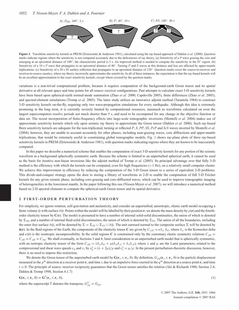
C) SS, 120◦, 20 sB) P , 40◦, 10 sA) Pdiff, 100◦, 5 s

??

?

?

Figure 1. Traveltime sensitivity kernels in PREM (Dziewonski & Anderson 1981), calculated using the ray-based approach of Dahlen et al. (2000). Questionmarks indicate regions where the sensitivity is not computed accurately due to the deficiencies of ray theory. (a) Sensitivity of a P wave grazing the core andemerging at an epicentral distance of 100◦; the characteristic period is 5 s. An improved method is needed to compute the sensitivity in the D′′ region. (b)Sensitivity of a 10 s P wave that propagates to an epicentral distance of 40◦. Turning P and S waves at this distance and less are affected by upper-mantletriplications. (c) Sensitivity of a 20 s SS surface reflection that propagates to an epicentral distance of 120◦. Question marks cover the source-to-receiver andreceiver-to-source caustics, where ray theory incorrectly approximates the sensitivity. In all of these instances, the expectation is that the ray-based kernels willbe an excellent approximation to the exact sensitivity kernels, except where covered by the question marks.

variations is a non-trivial computational problem, because it requires computation of the background-earth Green tensor and its spatialderivative at all relevant space and time points for all source–receiver configurations. Past attempts to calculate exact 3-D sensitivity kernelshave been based upon spherical-earth normal-mode summation (Zhao et al. 2000; Capdeville 2005), finite differences (Zhao et al. 2005),and spectral-element simulations (Tromp et al. 2005). The latter study utilizes an innovative adjoint method (Tarantola 1984) to construct3-D sensitivity kernels on-the-fly, requiring only two wave-propagation simulations for every earthquake. Although this idea is extremelypromising in the long term, it is currently severely limited by computational resources, inasmuch as waveforms calculated on even thelargest supercomputers resolve periods not much shorter than 5 s, and need to be recomputed for any change in the objective function ordata set. The recent incorporation of finite-frequency effects into large-scale tomographic inversions (Montelli et al. 2004) makes use ofapproximate sensitivity kernels which rely upon seismic ray theory to approximate the Green tensor (Dahlen et al. 2000). Such ray-basedBorn sensitivity kernels are adequate for the non-triplicated, turning or reflected P, S, PP, SS, PcP and ScS waves inverted by Montelli et al.(2004); however, they are unable to account accurately for other phases, including near-grazing waves, core diffractions and upper-mantletriplications, that would be extremely useful in constraining global tomographic models. Fig. 1 shows ray-plane plots of three ray-basedsensitivity kernels in PREM (Dziewonski & Anderson 1981), with question marks indicating regions where they are known to be inaccuratelycomputed.

In this paper we describe a numerical scheme that enables the computation of exact 3-D sensitivity kernels for any portion of the seismicwaveform in a background spherically symmetric earth. Because the scheme is limited to an unperturbed spherical earth, it cannot be usedas the basis for iterative non-linear inversions like the adjoint method of Tromp et al. (2005). Its principal advantage over that fully 3-Dmethod is the efficiency with which the kernels can be computed, even for high frequencies (>1 Hz), on a relatively small computer cluster.We achieve this improvement in efficiency by reducing the computation of the 3-D Green tensor to a series of equivalent 2-D problems.This divide-and-conquer strategy opens the door to storing a library of waveforms in 2-D to enable the computation of full 3-D Frechetkernels for any given seismic phase, including core-grazing and core-diffracted waves, which can be used to improve tomographic imagingof heterogeneities in the lowermost mantle. In the paper following this one (Nissen-Meyer et al. 2007), we will introduce a numerical methodbased on 2-D spectral elements to compute the spherical-earth Green tensor and its spatial derivative.

2 F I R S T - O R D E R P E RT U R B AT I O N T H E O RY

For simplicity, we ignore rotation, self-gravitation and anelasticity, and consider an unperturbed, anisotropic, elastic earth model occupying afinite volume ⊕ with surface ∂⊕. Points within the model will be labelled by their position r; we denote the mass density by ρ(r) and the fourth-order elasticity tensor by C(r). The model is presumed to have a number of internal solid-solid discontinuities, the union of which is denotedby �SS, and a number of internal fluid-solid discontinuities, the union of which is denoted by �FS. The union of all the boundaries, includingthe outer free surface ∂⊕, will be denoted by � = �SS ∪ �FS ∪ ∂⊕. The unit outward normal to the composite surface � will be denoted byn(r). In the fluid regions of the Earth, the components of the elasticity tensor C are given by C i jkl = κδ i j δkl , where δ i j is the Kronecker deltaand κ(r) is the isentropic incompressibility. In the solid regions C is constrained only by the customary elastic symmetry relations C ijkl =C jikl = C ijlk = C klij. We shall eventually, in Sections 3 and 4, limit consideration to an unperturbed earth model that is spherically symmetric,with an isotropic elasticity tensor of the form C ijkl = λδ i jδkl + µ(δ ikδ jl + δ ilδ jk), where λ and µ are the Lame parameters, related to thecompressional and shear wave speeds vp and v s by v2

p = (λ + 2µ)/ρ and v2s = µ/ρ. In the present perturbation-theoretic discussion, however,

there is no need to impose this restriction.We denote the Green tensor of the unperturbed earth model by G(rr, t ; rs, 0). By definition, G pq (rr, t ; rs, 0) is the particle displacement

measured in the pth direction at a receiver point rr and time t, due to an impulsive force exerted in the q th direction at a source point rs and timet = 0. The principle of source–receiver reciprocity guarantees that the Green tensor satisfies the relation (Aki & Richards 1980, Section 2.4;Dahlen & Tromp 1998, Section 4.1.7)

G(rr, t ; rs, 0) = GT(rs, t ; rr, 0), (1)

where the superscript T denotes the transpose, GTpq = Gqp .

C© 2007 The Authors, GJI, 168, 1051–1066

Journal compilation C© 2007 RAS

Spherical-earth Frechet sensitivity kernels 1053

Let u(t) be the p component of the displacement at the receiver rr due to a step-function, moment-tensor source MH(t) situated at thesource point rs. This moment-tensor response of the Earth is given in terms of the Green tensor by (Aki & Richards 1980, Section 3.3; Dahlen& Tromp 1998, Section 5.4.1)

u(t) =∫ t

0M :∇sG

T(rr, τ ; rs, 0) · p dτ, (2)

where ∇s denotes the gradient with respect to the source coordinates rs. For a more general earthquake source at rs, with a moment releasehistory m(t), 0 ≤ t ≤ ∞, satisfying∫ ∞

0m(t) dt = 1, (3)

where a dot denotes differentiation with respect to time, the displacement at rr is given by

u(t) =∫ ∞

0m(t − τ )uH (τ ) dτ, (4)

where uH (t) is the Heaviside response, given by eq. (2). We shall henceforth restrict attention to a step-function source m(t) = H (t), and dropthe subscript H upon the response u(t).

2.1 Volumetric perturbation

Suppose now that the earth model is subjected to pointwise infinitesimal perturbations in the density and elastic properties, ρ(r) → ρ(r) +δρ(r) and C(r) → C(r) + δC(r). The moment-tensor response is altered as a result of this slight perturbation, u(t) → u(t) + δu(t). The Bornapproximation provides an explicit linear relation between the waveform perturbation δu(t) and the volumetric model perturbations δρ(r) andδC(r). We do not provide an independent derivation of this well-known relationship (e.g. Chapman 2004, Section 10.3.1.2), but instead simplyquote the result here. Two unperturbed displacement fields are required at every volumetric ‘scatterer’ location r: the first is the response

u(r, t) =∫ t

0M :∇sG

T(r, τ ; rs, 0) dτ (5)

to the earthquake MH (t) situated at the source location rs, and the second is the response←u (r, t) = G(r, t ; rr, 0) · p. (6)

to an impulsive point force p δ(t) exerted in the receiver polarization direction at rr. Differentiation with respect to t and r yields the associateddisplacement and strain fields→v (r, t) = ∂t

→u (r, t),

→E (r, t) = 1

2

[∇→

u (r, t) + ∇→u (r, t)T

], (7)

←v (r, t) = ∂t

←u (r, t),

←E (r, t) = 1

2

[∇←

u (r, t) + ∇←u (r, t)T

]. (8)

The forward-pointing and backward-pointing arrows serve as a mnemonic reminder that the fields u→

, v→

and E→

are considered to propagate in

the forward direction from rs to r, whereas←u,

←v and

←E are considered to propagate in the backward direction from rr to r. The perturbation

δu(t) is given in terms of δρ(r) and δC(r) by (Chapman 2004, eq. 10.3.42)

δu(t) = −∫

⊕d3r δρ(r)

∫ t

0

→v (r, τ ) · ←

v (r, t − τ ) dτ −∫

⊕d3r

∫ t

0

→E (r, τ ) :δC(r) :

←E (r, t − τ ) dτ. (9)

Making use of an obvious index notation and suppressing all of the dependencies, we can rewrite this in the abbreviated form

δu = −∫

⊕

[δρ

→vi ∗ ←

vi +δCi jkl

→Ei j ∗

←Ekl

]d3r, (10)

where ∗ denotes time-domain convolution. The physical signal u(t) + δu(t) propagates entirely in the forward direction, from the source rs

to the scatterer r and then to the receiver rr. We have made use of the reciprocity relation (1) to express the results (9) and (10) in terms of the

backward-propagating velocity←v = ←

v i xi and strain←E = ←

Ekl xk xl at the scatterer r.

2.2 Boundary perturbation

Suppose next that, in addition to the volumetric perturbations δρ and δC, the boundary � is displaced outward (i.e. in the n direction) by aninfinitesimal amount δd(r). In that case, eq. (10) must be supplemented by a boundary integral term (Dahlen 2005):

δu = −∫

⊕

[δρ

→v i ∗ ←

v i +δCi jkl

→Ei j ∗

←Ekl

]d3r

+∫

�

δd[ρ

→v i ∗ ←

v i + Ci jkl

→Ei j ∗

←Ekl −ni Ci jkl

←Ekl ∗∂n

←u j − ni Ci jkl

←Ekl ∗∂n

→u j

]+

−d2r

−∫

�FS

δd[ni n j Ci jkl

←Ekl ∗∂ �

q

←u q + ni n j Ci jkl

←Ekl ∗∂ �

q

→u q + →

u q ∗∂ �q (ni n j Ci jkl

←Ekl ) + ←

u q ∗∂ �q (ni n j Ci jkl

←Ekl )

]+

−d2r, (11)

C© 2007 The Authors, GJI, 168, 1051–1066



0

x

y

z

rs

θs

xs

ys

north

φs

zs

south

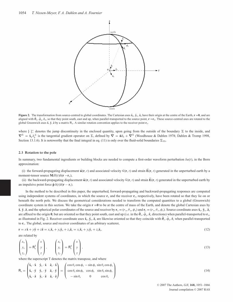
Figure 2. The transformation from source-centred to global coordinates. The Cartesian axes xs, ys, zs have their origin at the centre of the Earth, r =0, and arealigned with θs, φs, rs, so that they point south, east and up, when parallel-transported to the source point, r =rs. These source-centred axes are rotated to theglobal Greenwich axes x, y, z by a matrix Rs. A similar rotation convention applies to the receiver point rr.

where [· ]+− denotes the jump discontinuity in the enclosed quantity, upon going from the outside of the boundary � to the inside, and∇� = xq∂

�q is the tangential gradient operator on �, defined by ∇ = n∂n + ∇� (Woodhouse & Dahlen 1978; Dahlen & Tromp 1998,

Section 13.1.6). It is noteworthy that the final integral in eq. (11) is only over the fluid-solid boundaries �FS.

2.3 Rotation to the pole

In summary, two fundamental ingredients or building blocks are needed to compute a first-order waveform perturbation δu(t), in the Bornapproximation:

(i) the forward-propagating displacement u→

(r, t) and associated velocity v→(r, t) and strain E→

(r, t) generated in the unperturbed earth by amoment-tensor source MH (t)δ(r −rs),

(ii) the backward-propagating displacement u←(r, t) and associated velocity v←(r, t) and strain E←

(r, t) generated in the unperturbed earth byan impulsive point force p δ(t)δ(r − rr).

In the method to be described in this paper, the unperturbed, forward-propagating and backward-propagating responses are computedusing independent systems of coordinates, in which the source rs and the receiver rr, respectively, have been rotated so that they lie on orbeneath the north pole. We discuss the geometrical considerations needed to transform the computed quantities to a global (Greenwich)coordinate system in this section. We take the origin r =0 to be at the centre of mass of the Earth, and denote the global Cartesian axes byx, y, z, and the spherical polar coordinates of the source and receiver by rs = (r s, θ s, φ s) and rr = (r r, θ r, φ r). Source coordinate axes xs, ys, zs

are affixed to the origin 0, but are oriented so that they point south, east and up (i.e. in the θs, φs, rs directions) when parallel-transported to rs,as illustrated in Fig. 2. Receiver coordinate axes xr, yr, zr are likewise oriented so that they coincide with θr, φr, rr when parallel-transportedto rr. The global, source and receiver coordinates of an arbitrary scatterer,

r = x x + yy + zz = xsxs + ysys + zszs = xrxr + yryr + zrzr, (12)

are related by

xs

ys

zs

= RT

s

x

y

z

,

xr

yr

zr

= RT

r

x

y

z

, (13)

where the superscript T denotes the matrix transpose, and where

Rs =

xs · x ys · x zs · x

xs · y ys · y zs · y

xs · z ys · z zs · z

=

cos θs cos φs − sin φs sin θs cos φs

cos θs sin φs cos φs sin θs sin φs

− sin θs 0 cos θs

(14)

C© 2007 The Authors, GJI, 168, 1051–1066



and

Rr =

xr · x yr · x zr · x

xr · y yr · y zr · y

xr · z yr · z zr · z

=

cos θr cos φr − sin φr sin θr cos φr

cos θr sin φr cos φr sin θr sin φr

− sin θr 0 cos θr

(15)

are the rotation matrices that rotate the source rs and the receiver rr to the north pole.Suppose we have the capability of computing the components

→vs =

xs · →v

ys · →v

zs · →v

,

→Es =

xs·→E · xs xs·

→E · ys xs·

→E · zs

ys·→E · xs ys·

→E · ys ys·

→E · zs

zs·→E · xs zs·

→E · ys zs·

→E · zs

(16)

of the forward-propagating velocity and strain fields v→

(r, t) and E→

(r, t) in the source coordinate system xs, ys, zs. The corresponding components

→v =

x · →v

y · →v

z · →v

,

→E =

x · →E · x x · →

E · y x · →E · z

y · →E · x y · →

E · y y · →E · z

z · →E · x z · →

E · y z · →E · z

(17)

in the global coordinate system x, y, z are given by the usual transformation relations→v = RT

s

→vs,

→E = RT

s

→Es Rs. (18)

The receiver-coordinate components

←vr =

xr · ←v

yr · ←v

zr · ←v

,

←Er =

xr ·←E · xr xr·

←E · yr xr ·

←E · zr

yr ·←E · xr yr·

←E · yr yr ·

←E · zr

zr ·←E · xr zr·

←E · yr zr ·

←E · zr

(19)

of the backward-propagating velocity and strain fields v←

(r, t) and E←

(r, t) are likewise related to the global-coordinate components

←v =

x · ←v

y · ←v

z · ←v

,

←E =

x · ←E · x x · ←

E · y x · ←E · z

y · ←E · x y · ←

E · y y · ←E · z

z · ←E · x z · ←

E · y z · ←E · z

(20)

by←v = RT

r

←vr,

←E = RT

r

←Er Rr. (21)

2.4 Computational outline

To conclude this section, we outline the steps needed to compute a first-order waveform perturbation δu(t):

(i) Compute the matrices Rs, Rr that rotate the source and receiver rr, rs to the pole.(ii) Find the source and receiver coordinates of a selected scatterer r = (x , y, z).(iii) Compute the unperturbed, forward-propagating velocity v

→s and strain E

→s.

(iv) Compute the unperturbed, backward-propagating velocity v←

r and strain E←

r.(v) Transform v

→s, E

→s and v

←r, E

←r to global coordinates v

→, E

→and v

←, E

←.

(vi) Use v→

, E→

and v←

, E←

to compute the convolutions −δρ v→

i ∗ v←

i − δCijklE→

i j ∗ E←

kl.(vii) Additional convolutions are required if there are also boundary perturbations δd.(viii) Repeat for all scatterers r and integrate over ⊕ and � to find δu(t).

Steps (iii) and (iv) are the crux of the calculation. Fundamentally, we need to be able to compute the forward-propagating displacementfield u

→and its temporal and spatial derivatives v

→, E

→in a system of coordinates with the source rs rotated to the north pole, and the backward-

propagating displacement field u←

and its temporal and spatial derivatives v←

, E←

in a system of coordinates with the receiver rs rotated to thenorth pole. A numerical scheme for conducting such calculations is, in fact, the central topic of this paper; so far, all we have done is articulateour principal motivation for developing such a scheme.

3 S N R E I E A RT H M O D E L

We shall, in our numerical scheme, restrict attention to an unperturbed SNREI earth model, having spherical boundaries � = �SS ∪ �FS ∪∂⊕, with unit normal everywhere equal to the radial vector, n = r. The density ρ, fluid incompressibility κ , solid Lame parameters λ and µ,

C© 2007 The Authors, GJI, 168, 1051–1066



and compressional and shear wave speeds vp and v s are all functions only of radius r = ‖r‖. The source rs and receiver rr will henceforthalways be considered to lie on or beneath the north pole. The subscripts s and r will be dropped from the coordinate axes xs, ys, zs and xr, yr, zr,for simplicity, and the spherical polar coordinates of an arbitrary scatterer will now be denoted simply by r = (r , θ , φ). The polar coordinatesof the source and receiver are rs = (r s, 0, · ) and rr = (r r, 0, · ), where the dots are indicative of the indeterminateness of the longitude φ atthe pole. In any realistic whole-earth application, the receiver will be situated on the free surface, so that r r = r 0, the radius of the Earth. Theearthquake moment tensor M and receiver polarization vector p will be expressed in terms of their x, y, z components in the form

M = Mxx xx + Myy yy + Mzz zz + Mxy(xy + yx) + Mxz(xz + zx) + Myz(yz + zy), (22)

p = px x + py y + pz z. (23)

In this notation, Mxz and Myz correspond to θs · M · rs and φs · M · rs at the global source location rs, and px , p y , pz point to the south, eastand up (i.e. in the θr, φr and rr directions) at the global receiver location rr.

3.1 Mode-sum representation of the response

The response of a spherically symmetric, non-rotating, elastic earth model to a polar moment-tensor or point-force source MH (t) or p δ(t)can be expressed as a sum over the normal modes of free oscillation. We review this mode-sum representation of the response in what follows,since it provides a useful guide to the expected form of the alternative solution which we seek to develop. The results in this section are notrestricted to a SNREI earth model, but are applicable to any elastic earth model that is invariant with respect to rigid rotations about its centre.We adopt the normal-mode nomenclature of Dahlen & Tromp (1998), denoting the eigenfrequency of a mode of angular degree l = 0, 1, . . .

and overtone number n = 0, 1, . . . by nωl , and normalizing the associated spheroidal and toroidal eigenfunctions by∫ r0

0

[nU 2

l (r ) + n V 2l (r ) + n W 2

l (r )]

r 2 dr = 1. (24)

The forward-propagating response to a step-function moment-tensor source is of the form (Dahlen & Tromp 1998, eq. 4.67)

→u (r, t) =

∞∑n=0

∞∑l=0

nω−2l n

→A l (r) [1 − cos(nωl t)] , (25)

whereas the backward-propagating response to an impulsive point force is of the form (Dahlen & Tromp 1998, eq. 4.60)

←u (r, t) =

∞∑n=0

∞∑l=0

nω−1l n

←A l (r) sin(nωl t). (26)

The vector amplitude factors nA→

l (r) and nA←

l (r) describing the shape of every spherical-earth oscillation are given by (Dahlen & Tromp 1998,eqs 10.52 and 10.60)

A↔

(r, θ, φ) =(

2l + 1

4π

) {rU (r ) + θk−1

[V (r )∂θ + W (r )(sin θ )−1∂φ

] + φk−1[V (r )(sin θ )−1∂φ − W (r )∂θ

] }A↔

(θ, φ), (27)

where the double-sided arrows point in either direction, and where we have let k = √l(l + 1) and dropped the subscripts n and l for simplicity.

The depth-independent, forward-propagating scalar n A→l (θ , φ) is a sum over surface spherical harmonics of degree l and orders 0 ≤ m ≤ 2

(Dahlen & Tromp 1998, eqs 10.53–10.59)→A = a0 Pl0(cos θ ) + Pl1(cos θ )(a1 cos φ + b1 sin φ) + Pl2(cos θ )(a2 cos 2φ + b2 sin 2φ), (28)

where

a0 = Mzz U ′s + (Mxx + Myy)r−1

s

(Us − 1

2 kVs

), (29)

a1 = k−1[Mxz(V′

s − r−1s Vs + kr−1

s Us) − Myz(W′s − r−1

s Ws)], (30)

b1 = k−1[Myz(V′

s − r−1s Vs + kr−1

s Us) + Mxz(W′s − r−1

s Ws)], (31)

a2 = k−1r−1s

[12 (Mxx − Myy)Vs − Mxy Ws

], (32)

b2 = k−1r−1s

[Mxy Vs + 1

2 (Mxx − Myy)Ws

]. (33)

The backward-propagating scalar←A(θ , φ) has an analogous form, except that the order is restricted to 0 ≤ m ≤ 1:

←A = c0 Pl0(cos θ ) + Pl1(cos θ )(c1 cos φ + d1 sin φ), (34)

where

c0 = pzUr, c1 = k−1(

px Vr − py Wr

), d1 = k−1

(py Vr + px Wr

). (35)

A prime in eqs (29)–(33) denotes differentiation with respect to radius r, and the subscripts s and r denote evaluation of U , V and W at thesource and receiver radii, r = r s and r = r r. The quantities Pl0, Pl1, Pl2 are the associated Legendre functions of degree l and orders m = 0,1, 2 (e.g. Dahlen & Tromp 1998, eq. B.48).

C© 2007 The Authors, GJI, 168, 1051–1066



3.2 Monopole, dipole and quadrupole sources

Inspection of the above results shows that the forward- and backward-propagating, spherical-earth responses u→

(r, t) and u←

(r, t) can be expressedas a linear superposition of three different types of sources, which can be distinguished on the basis of their azimuthal dependence on φ:

(i) monopole sources, for which u→

and u←

are independent of φ,(ii) dipole sources, for which u

→and u

←vary as cos φ or sin φ,

(iii) quadrupole sources, for which u→

and u←

vary as cos 2φ or sin 2φ.

The source-coordinate representation of the moment tensor M in eq. (22) can be rearranged to yield a representation of M in terms ofits monopole, dipole and quadrupole constituents:

M =monopole︷︸︸︷

Mzz zz + 12 (Mxx + Myy)(xx + yy) +

dipole︷︸︸︷Mxz(xz + zx) + Myz(yz + zy)

+ 12 (Mxx − Myy)(xx − yy) + Mxy(xy + yx)︸︷︷︸

quadrupole

. (36)

Likewise, the point force (23) is a sum of monopole and dipole sources:

p = pz z︸︷︷︸monopole

+ px x + py y︸︷︷︸dipole

. (37)

The dipole sources in eq. (36) as well as those in eq. (37) may be treated simultaneously, because the response u→

to an Myz source at longitudeφ is identical to the response to an Mxz source at longitude φ − π/2, and the response u

←to a p y source at longitude φ is identical to the

response to a px source at longitude φ − π/2. Likewise, the two quadrupole sources in eq. (36) may be treated simultaneously, since theresponse u

→to an Mxy source at longitude φ is identical to the response to a 1

2 (Mxx − Myy) source at longitude φ − π/4. Altogether, we canreconstruct the full forward- and backward-propagating displacement fields u

→(r, t) and u

←(r, t) by considering six independent source types:

(i) a pz monopole source,(ii) an Mzz monopole source,(iii) a 1

2 (Mxx + Myy) monopole source,(iv) a px or p y dipole source,(v) an Mxz or Myz dipole source,(vi) a 1

2 (Mxx − Myy) or Mxy quadrupole source.

We describe the preliminaries of a numerical scheme for solving these six types of source problems within a SNREI earth in the nextsection. The essential strategy is to effect a reduction in the dimension from 3-D to 2-D by accounting explicitly for the known azimuthaldependence of the responses u

→(r, t) or u

←(r, t) to a monopole, dipole or quadrupole source. The resulting 2-D integral equations can be solved

numerically within a D-shaped, planar, semicircular disk, as illustrated schematically in Fig. 3. The method we describe can be generalised toa transversely isotropic, spherically symmetric earth model such as PREM (Dziewonski & Anderson 1981).

4 R E D U C E D - D I M E N S I O N W E A K F O R M U L AT I O N

In what follows, we shall be obliged to pay closer attention to the distinction between the fluid and solid regions of the Earth than we havedone so far; to that end, we introduce some refinements in our notation. For simplicity, we shall restrict attention to SNREI earth models witha solid inner core, overlain by a fluid outer core, overlain by a solid mantle and crust, but with no surficial ocean. We shall henceforth usethree-letter symbols to label the various regions and the spherical boundaries that separate them:

SIC: solid inner core,FOC: fluid outer core,SMC: solid mantle-plus-crust,ICB: inner-core boundary,CMB: core–mantle boundary.

We shall also de-emphasize the distinction between the forward-propagating, moment-tensor and backward-propagating, point-force responses,using generic, arrowless symbols u, E, T to refer to the displacements, strains and stresses u

→, E

→, T

→and u

←, E

←, T

←.

4.1 Equations of motion

To find u (r, t) everywhere within the Earth, we must solve the usual strong form of the equations of motion,

ρ∂2t u = ∇ · T in SIC, (38)

ρ∂2t u = −∇ P in FOC, (39)

C© 2007 The Authors, GJI, 168, 1051–1066



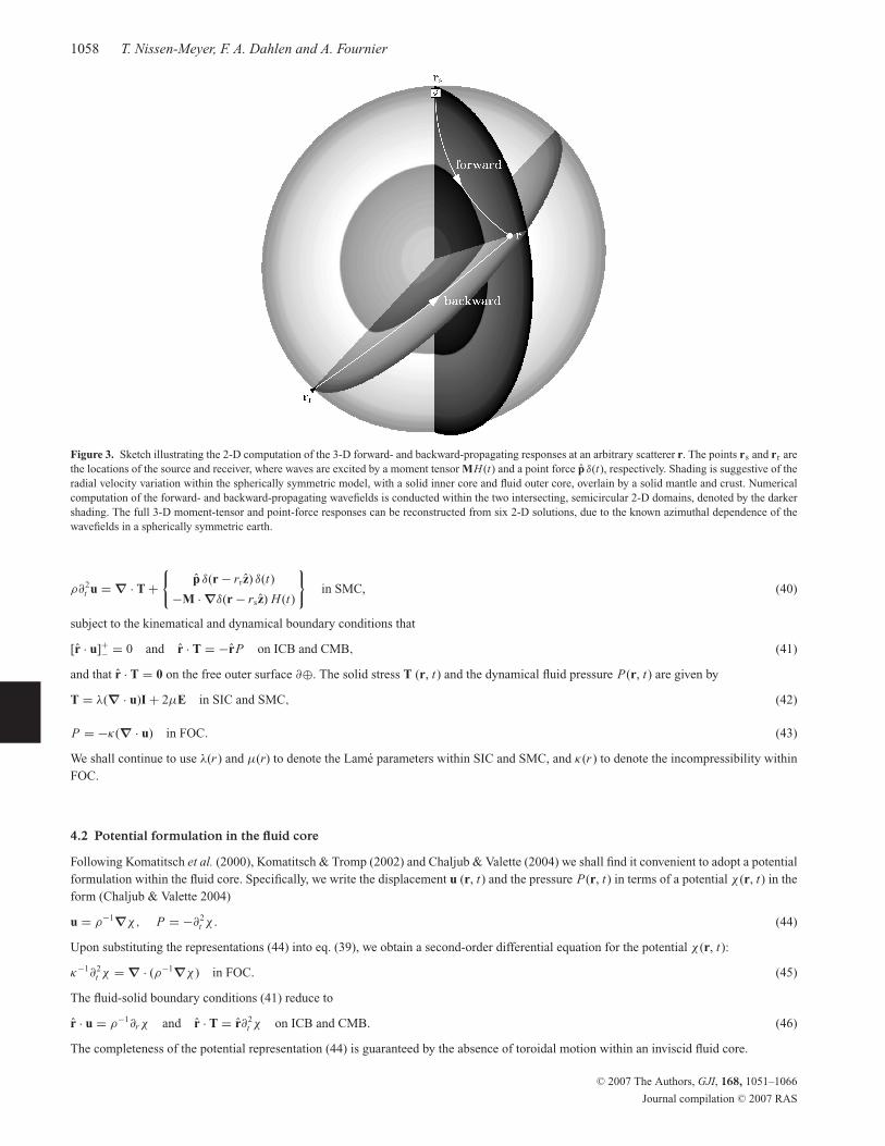
Figure 3. Sketch illustrating the 2-D computation of the 3-D forward- and backward-propagating responses at an arbitrary scatterer r. The points rs and rr arethe locations of the source and receiver, where waves are excited by a moment tensor MH (t) and a point force p δ(t), respectively. Shading is suggestive of theradial velocity variation within the spherically symmetric model, with a solid inner core and fluid outer core, overlain by a solid mantle and crust. Numericalcomputation of the forward- and backward-propagating wavefields is conducted within the two intersecting, semicircular 2-D domains, denoted by the darkershading. The full 3-D moment-tensor and point-force responses can be reconstructed from six 2-D solutions, due to the known azimuthal dependence of thewavefields in a spherically symmetric earth.

ρ∂2t u = ∇ · T +

{p δ(r − rrz) δ(t)

−M · ∇δ(r − rsz) H (t)

}in SMC, (40)

subject to the kinematical and dynamical boundary conditions that

[r · u]+− = 0 and r · T = −rP on ICB and CMB, (41)

and that r · T = 0 on the free outer surface ∂⊕. The solid stress T (r, t) and the dynamical fluid pressure P(r, t) are given by

T = λ(∇ · u)I + 2µE in SIC and SMC, (42)

P = −κ(∇ · u) in FOC. (43)

We shall continue to use λ(r ) and µ(r) to denote the Lame parameters within SIC and SMC, and κ(r ) to denote the incompressibility withinFOC.

4.2 Potential formulation in the fluid core

Following Komatitsch et al. (2000), Komatitsch & Tromp (2002) and Chaljub & Valette (2004) we shall find it convenient to adopt a potentialformulation within the fluid core. Specifically, we write the displacement u (r, t) and the pressure P(r, t) in terms of a potential χ (r, t) in theform (Chaljub & Valette 2004)

u = ρ−1∇χ, P = −∂2t χ. (44)

Upon substituting the representations (44) into eq. (39), we obtain a second-order differential equation for the potential χ (r, t):

κ−1∂2t χ = ∇ · (ρ−1∇χ ) in FOC. (45)

The fluid-solid boundary conditions (41) reduce to

r · u = ρ−1∂rχ and r · T = r∂2t χ on ICB and CMB. (46)

The completeness of the potential representation (44) is guaranteed by the absence of toroidal motion within an inviscid fluid core.

C© 2007 The Authors, GJI, 168, 1051–1066



4.3 3-D weak formulation

To derive the integral or weak form of the above equations of motion, we dot eqs (38) and (40) with a test vector w (r), multiply eq. (45)by a test scalar w(r), and integrate by parts over the 3-D earth ⊕, making use of the fluid-solid boundary conditions (46) and the free-surface condition r · T = 0 on ∂⊕. A solution u, χ in an appropriate space with square-integrable derivatives is then sought such that,for all admissible w, w, the following three integral equalities (obtained after integration over SIC, FOC and SMC) hold in the order listedbelow:∫

SIC

[ρw · ∂2

t u + λ(∇ · w)(∇ · u) + 2µ∇w :E]

d3r −∫

ICB(r · w)∂2

t χ d2r = 0, (47)

∫FOC

[κ−1w∂2

t χ + ρ−1∇w · ∇χ]

d3r +∫

ICBw(r · u) d2r −

∫CMB

w(r · u) d2r = 0, (48)

∫SMC

[ρw · ∂2

t u + λ(∇ · w)(∇ · u) + 2µ∇w :E]

d3r +∫

CMB(r · w)∂2

t χ d2r ={

p · w(rrz) δ(t)

M :∇w(rsz) H (t)

}. (49)

The SIC, FOC and SMC eqs (47)–(49) are coupled by virtue of the boundary integrals over ICB and CMB. It is noteworthy that the sourceterms on the right side of eq. (49) only involve the test vector w(rrz) and its gradient ∇w(rsz) evaluated at the polar receiver and earthquakelocations. Eqs (47)–(49) are identical to eqs (24), (23) and (16) of Komatitsch & Tromp (2002), except that they used a velocity potentialrepresentation v = ∂ t u = −ρ−1∇χ , P = ∂ tχ rather than the displacement potential representation (44), first introduced by Chaljub & Valette(2004).

4.4 2-D computational domain

Our objective in the remainder of this paper is to reduce the 3-D weak formulation (47)–(49) to a collection of 2-D weak problems, one foreach of the six source types listed in Section 3.2. The computational domain for each of these problems is a planar, D-shaped region , witha boundary ∂ consisting of a straight left edge corresponding to the polar axis, and a semicircular boundary on the right corresponding tothe free surface of the 3-D earth, as illustrated in Fig. 4. We shall continue to refer to the various solid and fluid subdomains by SIC, FOC andSMC, and to the semicircular boundaries separating them as ICB and CMB. Following Bernardi et al. (1999), Gerritsma & Phillips (2000)and Fournier et al. (2004, 2005) we shall employ a system of cylindrical polar coordinates s, z related to the spherical polar coordinates ineqs (27)–(28) by

s = r sin θ, z = r cos θ, r =√

s2 + z2, θ ={

arctan(s/z) if z ≥ 0,

arctan(s/z) + π if z < 0,(50)

The unit vectors s, z are Cartesian axes within the 2-D computational domain = SIC ∪ FOC ∪ SMC, with an origin 0 at the centre of theEarth. The unit radial vector on ICB and CMB is given by

r = s sin θ + z cos θ = s s + zz√s2 + z2

. (51)

We consider monopole, dipole and quadrupole sources separately, in the next three sections.

4.5 Monopole source

Inspection of the mode-sum eqs (25)–(35) shows that the response u (r, t), χ (r, t) to a pz , Mzz or 12 (Mxx + Myy) monopole source is of the

form

u = s us(s, z, t) + z uz(s, z, t), χ = χ (s, z, t). (52)

We choose time-independent test functions w(r), w(r) of the same form, i.e.

w = s ws(s, z) + z wz(s, z), w = w(s, z). (53)

To reduce the dimensionality of the weak formulation (47)–(49), we substitute the monopole representations (52)–(53), employ the cylindricalpolar formula for the gradient operator, ∇ = s ∂s + z ∂z + φ s−1∂φ , and the cylindrical divergence operator, ∇ ·u = (

∂s + s−1)

us +s−1∂φuφ +∂zuz , and evaluate the integrals

∫ 2π

0 dφ = 2π over the longitude φ. This yields a 2-D system of weak equations governing the three unknownsus(s, z, t), u z(s, z, t) and χ (s, z, t), which are equivalent to the 3-D system (47)–(49):∫

SIC

[ρ(ws∂

2t us + wz∂

2t uz) + λ(∂sws + ∂zwz + s−1ws)(∂sus + ∂zuz + s−1us)

+2µ(∂sws∂sus + ∂zwz∂zuz + s−2wsus) + µ(∂swz + ∂zws)(∂suz + ∂zus)]s ds dz

−∫

ICB

(sws + zwz√

s2 + z2

)∂2

t χ s ds dz = 0, (54)

C© 2007 The Authors, GJI, 168, 1051–1066



φ

s

z

polar axis

SIC

SMC

free surface

FOC

CMB

ICB

Figure 4. Planar 2-D computational domain composed of the subdomains SIC, FOC and SMC, with intervening fluid-solid boundaries ICB and CMB; thecylindrical coordinates s, φ, z are indicated. The outer boundary ∂ consists of two portions, a semicircular arc on the right corresponding to the free surface,where the boundary condition r · T = 0 is automatically satisfied in the weak formulation, and a straight left edge, corresponding to the polar axis passingthrough the 3-D earth. Special attention must be paid to this axis, because of the presence of divergent factors such as s−1 and s−2 in the governing 2-D integraleqs (54)–(56), (61)–(63) and (69)–(71).

∫FOC

[κ−1w∂2

t χ + ρ−1(∂sw∂sχ + ∂zw∂zχ )]

s ds dz

+∫

ICBw

(sus + zuz√

s2 + z2

)s ds dz −

∫CMB

w

(sus + zuz√

s2 + z2

)s ds dz = 0, (55)

2π

∫SMC

[ρ(ws∂

2t us + wz∂

2t uz

) + λ(∂sws + ∂zwz + s−1ws

)(∂sus + ∂zuz + s−1us

)+ 2µ

(∂sws∂sus + ∂zwz∂zuz + s−2wsus

) + µ(∂swz + ∂zws

)(∂suz + ∂zus

)]s ds dz

+ 2π

∫CMB

(sws + zwz√

s2 + z2

)∂2

t χ s ds dz =

pz wz(0, rr) δ(t)

Mzz ∂zwz(0, rs) H (t)

12 (Mxx + Myy)

[2∂sws(0, rs)

]H (t)

. (56)

As the braces in the final term indicate, eqs (54)–(56) are actually three independent coupled systems of equations, one for each of the threedifferent types of monopole sources, pz , Mzz and 1

2 (Mxx + Myy). We present a detailed derivation of the 12 (Mxx + Myy) axial source term

2∂ sws in Appendix A.

4.6 Dipole source

We follow a similar 2-D reduction strategy in the case of a dipole source. From inspection of eqs (25)–(35), we can deduce that the solutionu (r, t), χ (r, t) must be of the form

u = [ s us(s, z, t) + z uz(s, z, t)] cos φ − φ uφ(s, z, t) sin φ, χ = χ (s, z, t) cos φ (57)

in the case of either a px or Mxz source, and of the form

u = [ s us(s, z, t) + z uz(s, z, t)] sin φ + φ uφ(s, z, t) cos φ, χ = χ (s, z, t) sin φ (58)

in the case of either a p y or Myz source. As noted in Section 3.2, the response to a p y or Myz source at longitude φ is the same as the responseto a px or Mxz source at longitude φ − π/2, so that the functions us , u z , uφ are identical in eqs (57) and (58). It is also noteworthy thatbecause of the factors cos φ and sin φ, the symbols us , u z , uφ do not have their usual meaning (i.e. they are not the s, z, φ components of the

C© 2007 The Authors, GJI, 168, 1051–1066



displacement u). We again choose test functions w (r), w(r) of the same form, namely

w = [ s ws(s, z) + z wz(s, z)] cos φ − φwφ(s, z) sin φ, w = w(s, z) cos φ (59)

or

w = [ s ws(s, z) + z wz(s, z)] sin φ + φwφ(s, z) cos φ, w = w(s, z) sin φ, (60)

substitute into the 3-D eqs (47)–(49), and evaluate the integrals, in this case,∫ 2π

0 cos2 φ dφ = ∫ 2π

0 sin2 φ dφ = π and∫ 2π

0 sin φ cos φ dφ = 0,over the longitude φ. The resulting 2-D system of weak equations for a dipole source are∫

SIC

{ρ(ws∂

2t us + wz∂

2t uz + wφ∂2

t uφ

) + λ[∂sws + ∂zwz + s−1(ws − wφ)

][∂sus + ∂zuz + s−1(us − uφ)

]+ 2µ

[∂sws∂sus + ∂zwz∂zuz + s−2(ws − wφ)(us − uφ)

]+ µ(∂swz + ∂zws)(∂suz + ∂zus)

+µ[∂swφ + s−1(ws − wφ)

][∂suφ + s−1(us − uφ)

]+ µ(∂zwφ + s−1ws)(∂zuφ + s−1us)

}s ds dz

−∫

ICB

(sws + zwz√

s2 + z2

)∂2

t χ s ds dz = 0, (61)

∫FOC

[κ−1w∂2

t χ + ρ−1(∂sw∂sχ + ∂zw∂zχ + s−2wχ )]

s ds dz

+∫

ICBw

(sus + zuz√

s2 + z2

)s ds dz −

∫CMB

w

(sus + zuz√

s2 + z2

)s ds dz = 0, (62)

π

∫SMC

{ρ(ws∂

2t us + wz∂

2t uz + wφ∂2

t uφ

) + λ[∂sws + ∂zwz + s−1(ws − wφ)

][∂sus + ∂zuz + s−1(us − uφ)

]+ 2µ

[∂sws∂sus + ∂zwz∂zuz + s−2(ws − wφ)(us − uφ)


+ µ[∂swφ + s−1(ws − wφ)

][∂suφ + s−1(us − uφ)

]+ µ(∂zwφ + s−1wz)(∂zuφ + s−1uz)

}s ds dz

+ π

∫CMB

(sws + zwz√

s2 + z2

)∂2

t χ s ds dz =

(px or py) w+(0, rr) δ(t)

(Mxz or Myz)[∂swz(0, rs) + ∂zw+(0, rs)

]H (t)

, (63)

where we have defined the auxiliary test functions

w±(s, z) = 12 [ws(s, z) ± wφ(s, z)]. (64)

We need only solve the 2-D weak eqs (61)–(63) once to find the response (57) to a px or Mxz source and the response (58) to a p y or Myz

source. The px , p y and Mxz, Myz axial source terms w+ and ∂ sw z + ∂ zw+ are derived in Appendix A.

4.7 Quadrupole source

The response u (r, t), χ (r, t) to a quadrupolar 12 (Mxx − Myy) source is of the form

u = [ s us(s, z, t) + z uz(s, z, t)] cos 2φ − φ uφ(s, z, t) sin 2φ, χ = χ (s, z, t) cos 2φ, (65)

whereas the response to an Mxy source is of the form

u = [ s us(s, z, t) + z uz(s, z, t)] sin 2φ + φ uφ(s, z, t) cos 2φ, χ = χ (s, z, t) sin 2φ. (66)

Choosing test functions w (r), w(r) of the same form, either

w = [ s ws(s, z) + z wz(s, z)] cos 2φ − φwφ(s, z) sin 2φ, w = w(s, z) cos 2φ (67)

or

w = [ sws(s, z) + zwz(s, z)] sin 2φ + φwφ(s, z) cos 2φ, w = w(s, z) sin 2φ, (68)

C© 2007 The Authors, GJI, 168, 1051–1066



and making use of the longitudinal identities∫ 2π

0 cos2 2φ dφ = ∫ 2π

0 sin2 2φ dφ = π and∫ 2π

0 sin 2φ cos 2φ dφ = 0, we obtain the 2-D weaksystem of equations governing a quadrupole source:∫

SIC

{ρ(ws∂

2t us + wz∂

2t uz + wφ∂2

t uφ

) + λ[∂sws + ∂zwz + s−1(ws − 2wφ)

][∂sus + ∂zuz + s−1(us − 2uφ)

]+ 2µ

[∂sws∂sus + ∂zwz∂zuz + s−2(ws − 2wφ)(us − 2uφ)


+ µ[∂swφ + s−1(2ws − wφ)

][∂suφ + s−1(2us − uφ)

]+ µ(∂zwφ + 2s−1ws)(∂zuφ + 2s−1us)

}s ds dz

−∫

ICB

(sws + zwz√

s2 + z2

)∂2

t χ s ds dz = 0. (69)

∫FOC

[κ−1w∂2

t χ + ρ−1(∂sw∂sχ + ∂zw∂zχ + 4s−2wχ )]

s ds dz

+∫

ICBw

(sus + zuz√

s2 + z2

)s ds dz −

∫CMB

w

(sus + zuz√

s2 + z2

)s ds dz = 0, (70)

∫SMC

{ρ(ws∂

2t us + wz∂

2t uz + wφ∂2

t uφ

) + λ[∂sws + ∂zwz + s−1(ws − 2wφ)

][∂sus + ∂zuz + s−1(us − 2uφ)

]+2µ

[∂sws∂sus + ∂zwz∂zuz + s−2(ws − 2wφ)(us − 2uφ)


+µ[∂swφ + s−1(2ws − wφ)

][∂suφ + s−1(2us − uφ)

]+ µ(∂zwφ + 2s−1wz)(∂zuφ + 2s−1uz)

}s ds dz

−π

∫ICB

(sws + zwz√

s2 + z2

)∂2

t χ s ds dz = [12 (Mxx − Myy) or Mxy

] [2∂sw+(0, rs)

]H (t). (71)

Once again, we relegate the derivation of the source term 2∂ sw+ to Appendix A.

4.8 Axial boundary conditions

Solutions us(s, z, t), u z(s, z, t), uφ(s, z, t), χ (s, z, t) to the weak eqs (54)–(56), (61)–(63) and (69)–(71) automatically satisfy the stress-freecondition r · T = 0 on the semicircular right segment of the computational boundary ∂ . Special attention must, however, be paid to thestraight left segment of ∂ , since it is a boundary of the 2-D computational domain that does not have a physical counterpart in the 3-Dearth model ⊕. The boundary conditions along this s → 0 axis can be readily deduced by considering the θ → 0 limit of the mode-sumsolution (25)–(35). The limiting behaviours of the associated Legendre equations in eqs (28) and (34) are (Dahlen & Tromp 1998, eq. B.62)

Pl0(cos θ ) ∼ 1, Pl1(cos θ ) ∼ 12 l(l + 1)θ, Pl2(cos θ ) ∼ 1

2 l(l + 1)(l + 2)(l − 1)θ 2. (72)

The asymptotic functional form of the unknown variables us , u z , uφ , χ and associated test functions ws , w z , wφ , w in the axial limit dependsupon the source type:pz , Mzz or 1

2 (Mxx + Myy) monopole source:

uz ∼ f (z, t), us ∼ f (z, t)s, χ ∼ f (z, t), (73)

wz ∼ f (z), ws ∼ f (z)s, w ∼ f (z), (74)

px , p y or Mxz, Myz dipole source:

u+ ∼ f (z, t), uz ∼ f (z, t)s, u− ∼ f (z, t)s2, χ ∼ f (z, t)s, (75)

w+ ∼ f (z), wz ∼ f (z)s, w− ∼ f (z)s2, w ∼ f (z)s, (76)

12 (Mxx − Myy) or Mxy quadrupole source:

u+ ∼ f (z, t)s, uz ∼ f (z, t)s2, u− ∼ f (z, t)s3, χ ∼ f (z, t)s, (77)

w+ ∼ f (z)s, wz ∼ f (z)s2, w− ∼ f (z)s3, w ∼ f (z)s, (78)

where, by analogy with eq. (64), we have defined

u±(s, z, t) = 12 [us(s, z, t) ± uφ(s, z, t)]. (79)

The s → 0 asymptotic properties (74), (76) and (78) of w z and w± = 12 (ws ± wφ) have been used in Appendix A to evaluate the various

source terms in eqs (56), (63) and (71).Similar axial considerations arise in the application of the Fourier-spectral element method to the Navier–Stokes equations governing

fluid flows in axisymmetric geometries (Lopez & Shen 1998; Lopez et al. 2002; Fournier et al. 2004, 2005). As in that fluid-dynamical context,

C© 2007 The Authors, GJI, 168, 1051–1066



it is important to distinguish the so-called essential axial boundary conditions, which are all of Dirichlet type and must be specifically imposedin using a Galerkin formulation such as the spectral-element method (Karniadakis & Sherwin 1999) to solve the 2-D weak equations, fromthe Neumann and other higher-order boundary conditions (termed natural), which simply describe the expected asymptotic behaviour of thenumerical solution and are implicitly satisfied. The essential s → 0 boundary conditions for the three different source types are

pz, Mzz or 12 (Mxx + Myy) monopole source: us = ws = 0, (80)

px , py or Mxz, Myz dipole source: uz = u− = wz = w− = 0, χ = w = 0, (81)

12 (Mxx − Myy) or Mxy quadrupole source: uz = u± = wz = w± = 0, χ = w = 0. (82)

The Dirichlet conditions (80)–(82) must be imposed by axial masking of the unknowns u z , u±, χ and test functions w z , w±, w in solving eqs(54)–(56), (61)–(63) and (69)–(71).

5 C O N C L U S I O N S

The principle of elastodynamic reciprocity enables the Frechet sensitivity kernel for a seismic waveform to be computed by temporal andspatial differentiation, followed by convolution, of two unperturbed wavefields: the forward-propagating displacement response u

→(r, t) to

a moment-tensor MH (t) at the source rs and the backward-propagating response u←

(r, t) to a point force p δ(t) at the receiver rr. In thispaper, we have described a divide-and-conquer strategy for computing the two responses u

→(r, t) and u

←(r, t) at all points r within a 3-D

spherically symmetric earth by solving six systems of coupled weak equations within a planar, 2-D semicircular domain to account for allpossible monopole, dipole and quadrupole, moment-tensor and point-force source types. The full 3-D responses u

→(r, t) and u

←(r, t) can be

reconstructed from the six 2-D solutions, together with the known azimuthal dependence of the waves excited by the various sources. Theseresults establish the foundation for the paper that follows (Nissen-Meyer et al. 2007), in which we develop and implement a spectral-elementmethod to solve the resulting 2-D weak equations. Our ultimate objective is the development of a flexible and efficient scheme for computingspherical-earth, finite-frequency sensitivity kernels for arbitrary seismic phases and source–receiver configurations, with an initial focus uponwaves that probe the highly heterogeneous and geodynamically interesting D′′ region above the Earth’s core–mantle boundary.

A C K N O W L E D G M E N T S

We wish to thank Guust Nolet and Brian Schlottmann for insightful discussions, and Raffaella Montelli for her assistance in plotting Fig. 1.Financial support for this work has been provided by the US National Science Foundation under Grants EAR-0105387 and EAR-0345996.

R E F E R E N C E S

Aki, K. & Richards, P., 1980. Quantitative Seismology: Theory and Methods,W.H. Freeman & Co., San Francisco, California.

Bernardi, C., Dauge, M. & Maday, Y., 1999. Spectral Methods for Ax-isymmetric Domains, Vol. 3 of Series in Applied Mathematics, Gauthier-Villars, Paris, Numerical algorithms and tests by Mejdi Azaıez.

Capdeville, Y., 2005. An efficient Born normal mode method to computesensitivity kernels and synthetic seismograms in the earth, Geophys. J.Int., 163, 639–646.

Chaljub, E. & Tarantola, A., 1997. Sensitivity of SS precursors to topogra-phy on the upper-mantle 660 km discontinuity, Geophys. Res. Lett., 24,2613–2616.

Chaljub, E. & Valette, B., 2004. Spectral element modeling of three di-mensional wave propagation in a self-gravitating Earth with an arbitrarilystratified outer core, Geophys. J. Int., 158, 131–141.

Chapman, C., 2004. Fundamentals of Seismic Wave Propagation, CambridgeUniversity Press, Cambridge.

Dahlen, F.A., 2005. Finite-frequency sensitivity kernels for boundary topog-raphy perturbations, Geophys. J. Int., 162, 525–540.

Dahlen, F.A. & Baig, A., 2002. Frechet kernels for body wave amplitudes,Geophys. J. Int., 150, 440–466.

Dahlen, F.A. & Tromp, J., 1998. Theoretical Global Seismology, PrincetonUniversity Press, Princeton, New Jersey.

Dahlen, F.A., Hung, S.-H. & Nolet, G., 2000. Frechet kernels forfinite-frequency traveltimes—I. Theory, Geophys. J. Int., 141, 175–203.

Davaille, A., 1999. Simultaneous generation of hotspots and superswellsby convection in a heterogenous planetary mantle, Nature, 402, 756–760.

Dziewonski, A. & Anderson, D., 1981. Preliminary Reference Earth Model,Phys. Earth planet. Inter., 25, 297–356.

Favier, N. & Chevrot, S., 2003. Sensitivity kernels for shear wavesplitting in transverse isotropic media, Geophys. J. Int., 153, 213–228.

Fournier, A., Bunge, H.-P., Hollerbach, R. & Vilotte, J.-P., 2004. Applica-tion of the spectral element method to the axisymmetric Navier-Stokesequation, Geophys. J. Int., 156, 682–700.

Fournier, A., Bunge, H.-P., Hollerbach, R. & Vilotte, J.-P., 2005. A Fourier-spectral element algorithm for thermal convection in rotating axisymmet-ric containers, J. Comp. Phys., 204, 462–489.

Gauthier, O., Virieux, J. & Tarantola, A., 1986. Two-dimensional nonlin-ear inversion of seismic waveforms—numerical results, Geophysics, 51,1387–1403.

Gerritsma, M. & Phillips, T., 2000. Spectral element methods for axisym-metric Stokes problems, J. Comp. Phys., 164, 81–103.

Gu, Y.J., Dziewonski, A.M. & Ekstrom, G., 2003. Simultaneous inversion formantle shear velocity and topography of transition zone discontinuities,Geophys. J. Int., 154, 559–583.

Hung, S.-H., Garnero, E., Chiao, L.-Y., Kuo, B.-Y. & Lay, T., 2005. Finite-frequency tomography of D′′ shear velocity heterogeneity beneath theCaribbean, J. geophys. Res., 110, doi:10.1029/2004JB003373.

Igel, H. & Weber, M., 1995. SH-wave propagation in the whole mantle usinghigh-order finite differences, Geophys. Res. Lett., 22, 731–734.

Igel, H. & Weber, M., 1996. P-SV wave propagation in the Earth’s mantleusing finite differences: application to heterogeneous lowermost mantlestructure, Geophys. Res. Lett., 23, 415–418.

Ishii, M., Dziewonski, A.M., Tromp, J. & Ekstrom, G., 2002. Joint inversionof normal-mode and body-wave data for inner-core anisotropy: 2. Possiblecomplexities, J. geophys. Res., 107, doi:10.1029/2001JB000713.

C© 2007 The Authors, GJI, 168, 1051–1066



Karniadakis, G.E. & Sherwin, S.J., 1999. Spectral/hp Element Methods forCFD, Oxford University Press, Oxford.

Kellogg, L.H., Hager, B.H. & van der Hilst, R.H., 1999. Com-positional stratification in the deep mantle, Science, 283, 1881–1884.

Kendall, J.-M., 2000. Seismic anisotropy in the boundary layers of the Earth’smantle, in Earth’s Deep Interior: Mineral Physics and Tomography fromthe Atomic to the Global Scale, pp. 149–175, eds Karato, S., Stixrude, L.,Liebermann, R.C., Masters, T.G. & Forte, A.M., Geophysical MonographSeries 117, American Geophysical Union.

Komatitsch, D. & Tromp, J., 2002. Spectral-element simulations ofglobal seismic wave propagation—I. Validation, Geophys. J. Int., 149,390–412.

Komatitsch, D., Barnes, C. & Tromp, J., 2000. Wave propagation near afluid-solid interface: A spectral element approach, Geophysics, 65, 623–631.

Lay, T. & Garnero, E., 2004. Core-mantle boundary structures and processes,in The State of the Planet: Frontiers and Challenges in Geophysics, edsSparks, R.S.J. & Hawkesworth, C.J., Geophysical Monograph 150, IUGGVolume 19, doi:10.1029/150GM04.

Lay, T., Garnero, E. & Williams, Q., 2004. Partial melting in a thermo-chemical boundary layer at the base of the mantle, Phys. Earth planet.Inter., 146, 441–467.

Lopez, J. & Shen, J., 1998. An efficient spectral-projection method for theNavier-Stokes equations in cylindrical geometries I. Axisymmetric cases,J. Comp. Phys., 139, 308–326.

Lopez, J., Marques, F. & Shen, J., 2002. An efficient spectral-projectionmethod for the Navier-Stokes equations in cylindrical geometries II. Threedimensional cases, J. Comp. Phys., 176, 384–401.

Luo, Y. & Schuster, G., 1991. Wave equation traveltime inversion, Geo-physics, 56, 645–653.

Marquering, H., Nolet, G. & Dahlen, F.A., 1998. Three-dimensional wave-form sensitivity kernels, Geophys. J. Int., 132, 521–534.

Montelli, R., Nolet, G., Dahlen, F.A., Masters, G., Engdahl, E.R. & Hung,

S.-H., 2004. Finite-frequency tomography reveals a variety of plumes inthe mantle, Science, 303, 338–343.

Ni, S., Helmberger, D. & Tromp, J., 2005. Three-dimensional structure ofthe african superplume from waveform modelling, Geophys. J. Int., 161,283–294.

Nissen-Meyer, T., Fournier, A. & Dahlen, F.A., 2007. A two-dimensionalspectral-element method for computing spherical-earth seismograms– I. Moment-tensor source, Geophys. J. Int., doi:10.1111/j.1365-246X.2006.03121.x.

Rost, S., Garnero, E., Williams, Q. & Manga, M., 2005. Seismic constraintson a possible plume root at the core-mantle boundary, Nature, 435, 666–669.

Tarantola, A., 1984. Inversion of seismic reflection data in the acoustic ap-proximation, Geophysics, 49, 1259–1266.

To, A., Romanowicz, B., Capdeville, Y. & Takeuchi, N., 2005. 3D effects ofsharp boundaries at the borders of the African and Pacific Superplumes:observation and modeling, Earth planet. Sci. Lett., 233, 137–153.

Tromp, J., Tape, C. & Liu, Q., 2005. Seismic tomography, adjoint meth-ods, time reversal and banana-doughnut kernels, Geophys. J. Int., 160,195–216.

Woodhouse, J.H. & Dahlen, F.A., 1978. The effect of a general asphericalperturbation on the free oscillations of the Earth, Geophys. J. R. astr. Soc.,53, 335–354.

Woodward, M.J., 1992. Wave-equation tomography, Geophysics, 57, 15–26.Yu, W.-C., Wen, L. & Niu, F., 2005. Seismic velocity structure in the Earth’s

outer core, J. geophys. Res., 110, doi:10.1029/2003JB002928.Zhao, L., Jordan, T. & Chapman, C.H., 2000. Three-dimensional Frechet

differential kernels for seismic delay times, Geophys. J. Int., 141, 558–576.

Zhao, L., Jordan, T., Olsen, K.B. & Chen, P., 2005. Frechet kernels for imag-ing regional earth structure based on three-dimensional reference models,Bull. seism. Soc. Am., 95, 2066–2080.

Zhou, Y., Dahlen, F.A. & Nolet, G., 2004. 3-D sensitivity kernels for surface-wave observables, Geophys. J. Int., 158, 142–168.

A P P E N D I X A : D E R I VAT I O N O F T H E A X I A L S O U RC E T E R M S

The 2-D systems of weak eqs (54)–(56), (61)–(63) and (69)–(71) are noteworthy in that they enable synthetic-seismogram computations for apoint-force or moment-tensor source p δ(r − rr) δ(t) or −M : ∇ δ(r −rs) H (t) situated on the axis s = 0. In contrast, only a monopole source,including a toroidal ring source artificially situated one grid point away from the axis, can be treated using a 2-D, axisymmetric finite-differencemethod based upon the strong form (Chaljub & Tarantola 1997; Igel & Weber 1995, 1996). Since the successful incorporation of a point-forceor moment-tensor source is the principal advantage of the present 2-D formulation, and since the source terms in eqs (56), (63) and (71) dependupon a systematic application of the axial boundary conditions (73)–(78), we present a detailed derivation here. All of the test functions w z ,ws , wφ and w± = 1

2 (ws ± wφ) in this appendix are evaluated on the axis, at either the receiver point rr = (r r, 0, ·) or the source point rs =(r s, 0, ·).A1 Monopole source

Both a pz and a Mzz source are straightforward; the axial source terms are, respectively, w z and ∂ zw z . In the case of a 12 (Mxx + Myy) source,

the source term is (xx + yy) :∇w, where

∇w = ss ∂sww + zz ∂zwz + φφ s−1ws + sz ∂swz + zs ∂zws . (A1)

Utilizing the elementary transformation formulae x = s cos φ − φ sin φ, y = s sin φ + φ cos φ, we obtain

(xx + yy) :∇w = (∂sws + s−1ws)(cos2 φ + sin2 φ) = 2∂sws, (A2)

where we have used the axial boundary condition ∂ sws = s−1 ws , which is equivalent to the second of eqs (74), to obtain the final relation.

A2 Dipole source

The source term for a px dipole source is

x · w = (s cos φ − φ sin φ) · [(s ws + z wz) cos φ − φwφ sin φ]

= ws cos2 φ + wφ sin2 φ = w+(cos2 φ + sin2 φ) + w−(cos2 φ − sin2 φ)

= w+, (A3)

C© 2007 The Authors, GJI, 168, 1051–1066



where we have used the axial boundary condition w− = 0. The source term for a p y source is

y · w = (s sin φ + φ cos φ) · [(s ws + z wz) sin φ + φwφ cos φ]

= ws sin2 φ + wφ cos2 φ = w+(sin2 φ + cos2 φ) + w−(sin2 φ − cos2 φ)

= w+, (A4)

which is identical to eq. (A3), as expected. The source term for an Mxz dipole source is (xz + zx) :∇w, where

∇w = [ss ∂sws + zz ∂zwz + φφ s−1(ws − wφ) + sz ∂swz + zs ∂zws] cos φ

−[sφ ∂swφ + φs s−1(ws − wφ) + zφ ∂zwφ + φz s−1wz] sin φ. (A5)

Utilizing x = s cos φ − φ sin φ, we obtain

(xz + zx) :∇w = (∂swz + ∂zws) cos2 φ + (s−1wz + ∂zwφ) sin2 φ

= 12 (∂swz + s−1wz + 2∂zw+)(cos2 φ + sin2 φ) + 1

2 (∂swz − s−1wz + 2∂zw−)(cos2 φ − sin2 φ)

= ∂swz + ∂zw+, (A6)

where we have used the axial boundary conditions ∂ zw z = s−1 w z and w− = 0. The source term for an Myz source is (yz + zy) :∇w, where

∇w = [ss ∂sws + zz ∂zwz + φφ s−1(ws − wφ) + sz ∂swz + zs ∂zws] sin φ

+[sφ ∂swφ + φs s−1(ws − wφ) + zφ ∂zwφ + φz s−1wz] cos φ. (A7)

Utilizing y = s sin φ + φ cos φ, we obtain

(yz + zy) :∇w = (∂swz + ∂zws) sin2 φ + (s−1wz + ∂zwφ) cos2 φ

= 1

2(∂swz + s−1wz + 2∂zw+)(sin2 φ + cos2 φ) + 1

2 (∂swz − s−1wz + 2∂zw−)(sin2 φ − cos2 φ)

= ∂swz + ∂zw+, (A8)

which is identical to eq. (A6).

A3 Quadrupole source

The axial source term for a 12 (Mxx − Myy) quadrupole source is (xx − yy) :∇w, where

∇w = [ss ∂sws + zz ∂zwz + φφ s−1(ws − 2wφ) + sz ∂swz + zs ∂zws] cos 2φ

−[sφ ∂swφ + φs s−1(2ws − wφ) + zφ ∂zwφ + φz (2s−1wz)] sin 2φ. (A9)

Utilizing x = s cos φ − φ sin φ and y = s sin φ + φ cos φ, we obtain

(xx − yy) :∇w = [∂sws − s−1(ws − 2wφ)] cos2 2φ + [∂swφ + s−1(2ws − wφ)] sin2 2φ

= (∂sw+ + s−1w+)(cos2 2φ + sin2 2φ) + (∂sw− − 3s−1w−)(cos2 2φ − sin2 2φ)

= 2∂sw+, (A10)

where we have used the axial boundary conditions ∂ sw+ − s−1 w+ = 0 and ∂ sw– − 3s−1 w−, which are equivalent to the first and third ofeqs (78). In the case of an Mxy source, eqs (A9) and (A10) are replaced by

∇w = [ss ∂sws + zz ∂zwz + φφ s−1(ws − 2wφ) + sz ∂swz + zs ∂zws] sin 2φ

+[sφ ∂swφ + φs s−1(2ws − wφ) + zφ ∂zwφ + φz (2s−1wz)] cos 2φ (A11)

and

(xx + yy) :∇w = [∂sws − s−1(ws − 2wφ)] sin2 2φ + [∂swφ + s−1(2ws − wφ)] cos2 2φ

= (∂sw+ + s−1w+)(sin2 2φ + cos2 2φ) + (∂sw− − 3s−1w−)(sin2 2φ − cos2 2φ)

= 2∂sw+, (A12)

so that the 12 (Mxx − Myy) and Mxy source terms are the same.

A4 Summary

In summary, the weak-form source terms for the six independent, 2-D problems listed in Section 3.2 are

(i) a pz monopole source: w z ,(ii) an Mzz monopole source: ∂ zw z ,(iii) a 1

2 (Mxx + Myy) monopole source: 2∂ sws ,

C© 2007 The Authors, GJI, 168, 1051–1066



(iv) a px or p y dipole source: ws ,(v) an Mxz or Myz dipole source: ∂ sw z + ∂ zw+,(vi) a 1

2 (Mxx − Myy) or Mxy quadrupole source: 2∂ sw+.

Three axial derivatives arise: ∂ sws in case (iii), ∂ sw z in case (v) and ∂ sw+ in case (vi). In every instance, the differentiated quantity ws ,w z or w+ is the only variable that varies linearly with s in the vicinity of the axis.

C© 2007 The Authors, GJI, 168, 1051–1066


Documents

Spherical‐earth Fréchet sensitivity kernels