SIMIODE - STUDENT VERSION Stiff Differential Equations

STUDENT VERSION

Stiff Differential Equations

Kurt Bryan

Department of Mathematics

Rose-Hulman Institute of Technology

Terre Haute IN U.S.

1 INTRODUCTION

Most real-world systems of ordinary differential equations (ODE’s) must be solved numerically, either

because no closed-form solution exists, or the solution is too unwieldy to manipulate symbolically.

“Stiffness” is a particular property that some systems of ODE’s have that makes them challenging

to solve numerically. Stiffness often reflects an essential disparity of scale in a physical system—

one facet of a physical system may evolve in time on a relatively slow scale, e.g., seconds, while

another facet of the same system evolves much more rapidly, e.g., microseconds. It might be the

slow scale/large time evolution of the system that interests us, but the rapidly changing aspect

of the system’s behavior demands the attention of the numerical method and makes long-term

simulations computationally expensive. Stiff systems are surprisingly common, but rarely talked

about in introductory ODE or numerical analysis courses.

We consider here a variety of straightforward examples that illustrate the essential idea behind

stiffness. The goal here is not a treatise on the theory of numerical methods for ODE’s and stiff

systems, but rather an intuitive and practical guide to what stiff ODE’s are and some ideas on how

to handle them. There are also some physical examples and exercises to illustrate how stiff systems

come about.

2 NUMERICAL METHODS FOR ODE’S REVIEW

Consider a first order initial value problem

y′(t) = f(t, y(t)) (1)

2 Stiff Differential Equations

for an unknown scalar function y(t), with initial condition y(t0) = a. You can consider t as time. It is

frequently the case that we can’t solve (1) explicitly and so must resort to numerical approximation.

Recall that Euler’s method is one of the simplest schemes for this computation, and is really just

repeated tangent line extrapolation. In the examples that follow we’ll often use Euler’s method to

illustrate, but the conclusions generally hold for any “explicit one-step” numerical method (defined

below).

In Euler’s method we choose a step size “h” with h > 0 for the independent variable t and then

construct a sequence of approximations yk ≈ y(tk) where tk = t0 + kh with k = 1, 2, . . ., as follows.

If h is sufficiently small the approximation

y′(t) ≈ y(t+ h)− y(t)

h(2)

should be accurate (in the limit h→ 0 the right side converges to y′(t), assuming y is differentiable).

The approximation (2) can be rearranged to

y(t+ h) ≈ y(t) + hy′(t)

and if y(t) satisfies (1) we then have

y(t+ h) ≈ y(t) + hf(t, y(t)). (3)

Equation (3) tells us how to extrapolate the solution forward from time t to time t + h, at least

approximately.

We can use (3) to approximate y(t) for t0 ≤ t ≤ T for some final time T = t0 + Mh with the

following algorithm, Euler’s Method:

1. Set y0 = a and counter k = 0. Set tk = t0 + kh.

2. Use (3) to generate yk+1, an approximation to y(tk+1), as

yk+1 = yk + hf(tk, yk). (4)

3. If tk = T (equivalently, k = M) stop and return y0, y1, . . . , yM . Otherwise, increment k ← k+1

and return to step 2.

The smaller the step size h, the better this algorithm “tracks” the true solution.

Example 2.1. Consider the classic “exponential decay” ODE

y′ = λy (5)

where λ < 0, with initial condition y(0) = 1. The true solution is y(t) = eλt.

For λ = −1 we have y(t) = e−t. If we approximate y(t) with Euler’s method on the interval

0 ≤ t ≤ 5 with step size h = 0.5, the situation is as shown in the left panel in Figure 1. Also shown

is the direction field for the ODE (5). When h is smaller, the Euler procedure tracks the direction

field or solution more accurately, as shown in the right panel of Figure 1.

Stiff Differential Equations 3

Figure 1. Euler approximation to y′ = −y solution, step sizes 0.5 (left) and 0.1 (right).

But now consider what happens if we solve (5) with λ = −3 and the same step size h = 0.5,

as shown in the left panel in Figure 2. The Euler approximation is very poor, and qualitatively

incorrect—the true solution is always positive, but the approximation is actually negative at times.

When λ = 5 the situation is even worse, as illustrated in the right panel of Figure 2, for although

the true solution decays smoothly to zero, Euler’s method is unstable—the iterates grow without

bound!

Figure 2. Euler approximation to y′ = −λy solution, step size 0.5, λ = 3 (left) and λ = 5 (right).

If you examine Euler’s method geometrically in relation to the direction field, it’s easy to see

what goes wrong. Although the true solution decays smoothly to zero for any λ < 0, when λ is

“very” negative the solution changes rapidly, with a rather steep rate of decay. Even if the current

iterate yk is exact, Euler steps that are too large end up extrapolating to a wildly incorrect value


(very negative). For this ODE, a large step size in Euler’s method yields an iteration that isn’t

simply inaccurate, but actually unstable.

2.1 Exercises

1. For the ODE (5) with y(0) = 1, show that Euler’s method produces iterates that satisfy

yk+1 = (1 + λh)yk, and that (given that y0 = 1)

yk = (1 + λh)k. (6)

2. Based on (6), for a fixed λ < 0 show that the condition |1 + λh| < 1 requires that h < 2/|λ| if

we want yk → 0 as k →∞ (so the iterates decay, just like the solution). What happens if this

condition is not met (h is too large?) What condition on h assures that the yk iterates actually

remain positive?

3. The Improved Euler Method replaces the formula (4) in Euler’s Method with the two-step

procedure

u = yk + hf(tk, yk)

yk+1 = yk +h

2(f(tk, yk) + f(tk+1, u)) (7)

and is generally more accurate than Euler’s Method.

Solve the ODE (5) with λ = −1 and y(0) = 1 using the Improved Euler method, with step

size h = 0.5 out to time t = 5. Look at the iterates y0, . . . , y10. Do they remain positive? Decay

to zero? Are they accurate? Repeat with λ = −3 and λ = −5 (step size h = 0.5). Does the

Improved Euler method suffer from the same stability problems as Euler’s method?

The moral here is that for many numerical methods and ODE’s, step sizes that are too large

result in more than just inaccurate iterates. The numerical solution actually becomes unstable and

“blows up”, even if the true solution decays. This is starting to get at what stiffness is about, but

it’s not the whole story. Stiffness is really a property possessed by a system of differential equations.

Let’s look at some more examples, now involving systems of ODE’s.

3 STIFF SYSTEMS OF ODE’S

A system of ODE’s can be written in a form similar to (1), namely

y′(t) = f(t,y(t)) (8)

where y(t) = 〈y1(t), . . . , yn(t)〉 is a vector-valued function taking values in Rn, whose components

are the functions of interest. The function f(t,y(t)) is a vector-valued function taking values in Rn

that indicates how to compute the derivative of each function yk(t) in terms of t and y(t). Euler’s

Method for such a system takes precisely the same form as the scalar version and is simply repeated

extrapolation on each component of y(t).


Example 3.1. Let’s start by considering a system of ODE’s of the form

y′1(t) = λ1y1(t) (9)

y′2(t) = λ2y2(t) (10)

for some constants λ1, λ2 < 0. In the framework of (8) we have f(t,y) = 〈λ1y1, λ2y2〉. Of course, this

“system” is in fact decoupled—each equation can be solved independently of the other. Nonetheless,

it will serve to illustrate the essential issue with stiff systems. The exact solution is y1(t) = y1(0)eλ1t

and y2(t) = y2(0)eλ2t.

Let’s use Euler’s Method to solve the system starting at time t0 = 0 with y1(0) = 0.5 and

y2(0) = 0.5. Let h be the step size, tk = kh, and let’s use yk1 and yk2 to denote the iterates produced

by Euler’s Method, as approximations to y1(tk) and y2(tk). Euler’s Method (8) for the system

(9)-(10) takes the form

yk+11 = (1 + λ1h)yk1 (11)

yk+12 = (1 + λ2h)yk2 . (12)

It’s easy to see then that yk1 = y1(0)(1 + λ1h)k and yk1 = y2(0)(1 + λ2h)k from Exercise 1 above.

Suppose that λ1 and λ2 are both negative, and recall Exercise 2 above. Both true solutions

decay to zero, but |1 + λjh| > 1 if h > 2/|λj |, and so ykj (here j = 1 or j = 2) will grow without

bound as the iteration counter k increases, which does not reflect a qualitatively (or quantitatively!)

accurate solution; Euler’s method will be unstable. This means the maximum step size we can

take is dictated by the smaller of the quantities 2/|λ1|, 2/|λ2|, that is, the larger of |λ1|, |λ2|. If, for

example, λ2 < λ1 < 0, it’s λ2 that dictates the largest permissible step size. But it may be the case

that we’re interested in the evolution of the system related to λ1, which occurs on a longer time

scale, long after the eλ2t part of the solution has decayed. Yet we’re forced to take tiny steps with

size less than 2/|λ2| to track this solution.

To illustrate, suppose λ1 = −1 and λ2 = −100. Then y1(t) = y1(0)e−t, while y2(t) = y2(0)e−100t.

Here y2(t) decays much more rapidly than y1(t) and very quickly will be insignificant in magnitude.

If we are interested in tracking the decay of y1(t), however, we have to continue to iterate (11) and

(12) in a stable manner, which requires h < 2/100, even though (11) itself would only require h < 2.

This means taking unnecessarily many more iterations to get out to a large enough time to see the

evolution of y(t). This system is (moderately)“stiff.”

Example 3.2. Of course in the above example it would make sense to solve (9) and (10) inde-

pendently, each with an appropriate step size, but most systems are not decoupled like this one.

Consider instead a slightly more complicated (but still linear) system of the form[y′1(t)

y′2(t)

]=

[−56 55

44 −45

][y1(t)

y2(t)

]. (13)

The eigenvalues and eigenvectors of the matrix on the right in (13) are λ1 = −1, λ2 = −100 with


corresponding eigenvectors v1 =< 〈1, 1〉 and v2 = 〈1,−0.8〉. As such, the general solution is

y(t) = c1e−t

[1

1

]+ c2e

−100t

[1

−0.8

]. (14)

Take initial conditions y1(0) = 0.5 and y2(0) = 0.5; these are slightly “rigged” initial conditions, to

illustrate the vital point, but we’ll consider something more typical below. We find that c1 = 0.5

and c2 = 0.0. The solution is

y(t) = 0.5e−t

[1

1

].

The e−100t portion isn’t even present in the true solution (and if it were, it would decay toward zero

long before the solution above would).

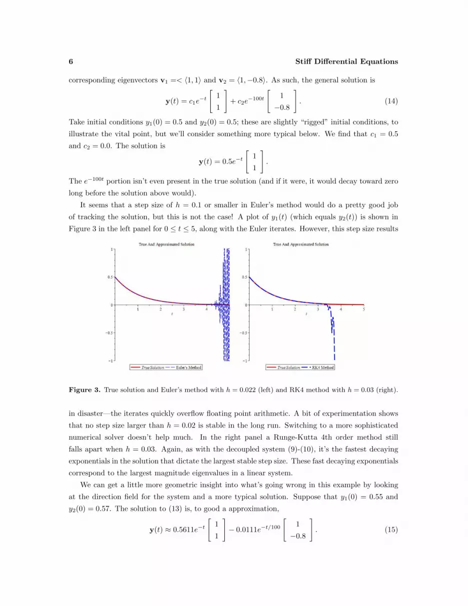
It seems that a step size of h = 0.1 or smaller in Euler’s method would do a pretty good job

of tracking the solution, but this is not the case! A plot of y1(t) (which equals y2(t)) is shown in

Figure 3 in the left panel for 0 ≤ t ≤ 5, along with the Euler iterates. However, this step size results

Figure 3. True solution and Euler’s method with h = 0.022 (left) and RK4 method with h = 0.03 (right).

in disaster—the iterates quickly overflow floating point arithmetic. A bit of experimentation shows

that no step size larger than h = 0.02 is stable in the long run. Switching to a more sophisticated

numerical solver doesn’t help much. In the right panel a Runge-Kutta 4th order method still

falls apart when h = 0.03. Again, as with the decoupled system (9)-(10), it’s the fastest decaying

exponentials in the solution that dictate the largest stable step size. These fast decaying exponentials

correspond to the largest magnitude eigenvalues in a linear system.

We can get a little more geometric insight into what’s going wrong in this example by looking

at the direction field for the system and a more typical solution. Suppose that y1(0) = 0.55 and

y2(0) = 0.57. The solution to (13) is, to good a approximation,

y(t) ≈ 0.5611e−t

[1

1

]− 0.0111e−t/100

[1

−0.8

]. (15)


The direction field for the system (13) is shown in Figure 4, along with a parametric plot of the true

solution y(t) (the black curve). Bear in mind that for aesthetic reasons, the arrows that delineate

the direction field are not drawn to scale—they are much longer than indicated in Figure 4. In

particular, the arrows that lie very far off the diagonal line y2 = y1 are rather long and point almost

orthogonally toward this line, a geometric manifestation of the fact that solutions like (14) decay

rapidly to a multiple of the vector 〈1, 1〉, and then slowly toward the origin.

Of course the true solution in this case does exactly this, starting at 〈0.55, 0.57〉 and quickly

decaying to the line y2 = y1. At all points the true solution curve follows the direction field (that’s

what it means to be a solution!) However, the Euler iterates (shown in blue/dashed) with step size

h = 0.022 do not behave like this. The first Euler step starts at 〈0.55, 0.57〉; at this point the vector

that dictates the direction the solution should go is 〈0.55,−1.45〉, but a step of h = 0.022 puts the

next iterate at 〈0.55, 0.57〉 + 0.022〈0.55, 1.45〉 ≈ 〈0.5621, 0.5381〉. This overshoots the line y2 = y1

and actually ends up farther off this line than the starting point 〈0.55, 0.57〉! This makes matters

even worse, for the direction field has an even larger magnitude here, and the next iterate overshoots

the other way. The process is repeated, with obvious effect. In every case, however, Euler’s method

is following the direction field toward the true solution, but due to the large magnitude of the

direction field (that stems from the large eigenvalue of −100) Euler overshoots and oscillates in an

unbounded manner.

The heart of the problem in this example is the large disparity in the magnitude of the eigenvalues.

The portion of the solution (14) corresponding to the −1 eigenvalue or e−t term dominates in most

cases, at least after a very short time, and the solution decays smoothly and gradually to zero.

But the portion of the solution corresponding to the eigenvalue of −100 is what limits the size of

the steps we can take, no matter how small that portion of the solution might be. In many stiff

systems one might encounter eigenvalues that vary over a much larger range, e.g., five or six orders

of magnitude, or more! We are then forced to take time steps perhaps one million times smaller

than the actual rate of change of the solution dictates. See Exercises 2 and 3 below.

This is the essence of stiffness, which does not have a precise or universally accepted definition.

Nonetheless, the general idea is

A system of ODE’s is stiff if the step size required to maintain stability in a numerical ODE

solver is small in relation to the scale on which the solution changes with respect to the

independent variable.

This can occur in a linear system x′ = Ax if the eigenvalues of A (real or complex) are of widely

varying magnitude. See Exercise 3 at the end for an example with complex eigenvalues. In a

nonlinear system the phenomena can be even more complicated; the solution may be stiff in some

intervals and not in others.

Modern numerical ODE solvers also incorporate “adaptive stepsizing.” That is, the step size h is

adjusted at each time step in order to control the (estimated) error of the solver at each step. When

things are going poorly, h is decreased. This can combat stiffness to some extent, but in practice


Figure 4. Euler iterates versus true solution and the direction field.

what ultimately happens is that h is reduced almost to 0 and the solver grinds to a halt. Another

approach to overcoming stiffness is needed.

4 THE IMPLICIT EULER METHOD

If a system is stiff, what can be done? One common solution is to use an “implicit” ODE solver.

Euler’s method and most other numerical methods encountered in an introductory ODE course are

“explicit, one-step” methods. What this means is that yk+1 is computed from the previous iterate

yk, the time tk, and the step size h (and the ODE itself, of course), in the form

yk+1 = yk + hφ(tk,yk, h) (16)

where φ(t,y, h) is a function of the indicated variables. For example, for an ODE (1) with Euler’s

method we have φ(t,y, h) = f(t,y). For the Improved Euler method we have (using (7)) φ(t,y, h) =12 (f(t,y) + f(t + h,y + hf(t,y))). The “explicit” refers to the fact that yk+1 is given explicitly in


(16). The “one-step” means that only yk (and not previous iterates yk−1,yk−2, etc.) are involved

in the right side of (16).

Explicit methods are convenient because we can “march” the iterates forward in time with a

minimum of fuss. Their drawback, for stiff systems, is that the step size h has to be small enough

to maintain stability of the method, even if the solution doesn’t change rapidly. An alternative is

to use an “implicit” method. These frequently remain stable for large (even arbitrarily large) step

sizes.

The simplest example of such a method is the implicit Euler method. The implicit version of

Euler’s method for a scalar ODE (1) replaces the approximation (2) with a so-called “backwards

difference”

y′(t) ≈ y(t)− y(t− h)

h(17)

(again, h > 0 here). The right side of (17) converges to y′(t) as h → 0, so if h is small enough the

approximation of (17) should be accurate. With t = tk (17) becomes y′(tk) ≈ (y(tk) − y(tk−1))/h,

which can be rearranged to y(tk) ≈ y(tk−1) + hy′(tk). Finally, if y satisfies (1) then we have

y(tk) ≈ y(tk−1) + hf(tk, y(tk)). If yk denotes our approximation to y(tk) this becomes a recipe for

how to compute yk, as a solution to yk = yk−1 +hf(tk, yk). Actually, we can shift indices k → k+ 1

and write the implicit Euler method as

yk+1 = yk + hf(tk+1, yk+1), (18)

a prescription for computing yk+1 from yk by solving (18). If f is sufficiently simple we might be

able to solve for yk+1 in closed-form, but in most cases we actually have to use a numerical method

(e.g., Newton’s method) just to obtain yk+1. Thus the implicit Euler’s method probably requires

more work at each iteration. The payback is that the method remains stable for large step sizes h.

Equation (18) generalizes to systems in an obvious way.

Example 4.1. To illustrate, let’s consider the ODE (5) again, with y(0) = 1, this time with the

implicit Euler method. In this case equation (18) yields yk+1 = yk−hλyk+1. Because f is so simple

here, we can actually solve for yk+1 in closed form as

yk+1 =yk

1 + λh.

With y0 = 1 its easy to see that in general

yk =1

(1 + λh)k. (19)

Contrast this to (6). In the case that λ = −5 and h is reasonably small, the implicit Euler method

does a good job of approximating the true solution. But even if h is large—say h = 0.5—the implicit

Euler method remains stable, and even positive, albeit a bit inaccurate. See Figure 5. In fact (19)

makes it clear that any step size h > 0 will yield such an approximation.


Figure 5. True solution and implicit Euler’s method with h = 0.5.

Example 4.2. To further illustrate, let’s apply the implicit Euler Method to the system (13). As

with standard Euler’s method, the implicit approach extends to a system of n ODE’s (8) in n

unknowns and leads to

yk+1 = yk + hf(tk+1,yk+1), (20)

a system of n (possibly nonlinear) equations in n unknowns, the components of the vector yk+1.

For the system y′ = Ay of (13) this means we must solve

yk+1 = yk + hAyk+1 (21)

to compute yk+1 from yk at each iteration. This is equivalent to solving (I − hA)yk+1 = yk for

yk+1, a linear system of equations that can be handled by Gaussian elimination or any linear solver.

This is a fortunate consequence of the fact that our ODE’s here are linear. In general the resulting

equations for yk+1 could be nonlinear and something like Newton’s method might be needed.

In fact in this case since A has eigenvalues −1 and −100, the matrix I−hA has nonzero positive

eigenvalues 1 + h and 1 + 100h if h > 0. Thus I − hA must be invertible and so (21) will have a

unique solution for yk+1.

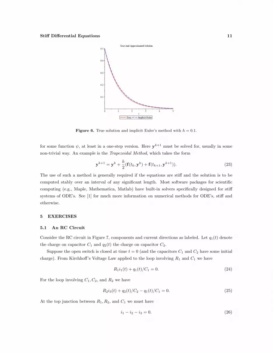
Figure 6 shows the result of this iteration, a plot of the true solution y1(t) = e−t and the implicit

Euler iterates for y1 with step size h = 0.1. Contrast this with the results of Figure 3. We can get

away with a much larger step size here and still maintain stability. An excessively large step size

will still result in a poor approximation though, just one that doesn’t blow up!

SUMMARY

There are many other implicit methods for systems of ODE’s. These methods often take the form

ψ(yk+1,yk, tk, tk+1) = 0, (22)


Figure 6. True solution and implicit Euler’s method with h = 0.1.

for some function ψ, at least in a one-step version. Here yk+1 must be solved for, usually in some

non-trivial way. An example is the Trapezoidal Method, which takes the form

yk+1 = yk +h

2(f(tk,y

k) + f(tk+1,yk+1)). (23)

The use of such a method is generally required if the equations are stiff and the solution is to be

computed stably over an interval of any significant length. Most software packages for scientific

computing (e.g., Maple, Mathematica, Matlab) have built-in solvers specifically designed for stiff

systems of ODE’s. See [1] for much more information on numerical methods for ODE’s, stiff and

otherwise.

5 EXERCISES

5.1 An RC Circuit

Consider the RC circuit in Figure 7, components and current directions as labeled. Let q1(t) denote

the charge on capacitor C1 and q2(t) the charge on capacitor C2.

Suppose the open switch is closed at time t = 0 (and the capacitors C1 and C2 have some initial

charge). From Kirchhoff’s Voltage Law applied to the loop involving R1 and C1 we have

R1i1(t) + q1(t)/C1 = 0. (24)

For the loop involving C1, C2, and R2 we have

R2i3(t) + q2(t)/C2 − q1(t)/C1 = 0. (25)

At the top junction between R1, R2, and C1 we must have

i1 − i2 − i3 = 0. (26)


Figure 7. Two loop RC circuit.

Finally, we also have

q′1 = i2 (27)

q′2 = i3. (28)

Using (26) to eliminate i1 in (24)-(25), then (27)-(28) to replace i2, i3, and finally solving for q′1 and

q′2 leads to

q′1(t) = −(

1

R2C1+

1

R1C2

)q1(t) +

1

R2C2q2(t) (29)

q′2(t) =1

R2C1q1(t)− 1

R2C2q2(t) (30)

a linear system of ODE’s for functions q1(t), q2(t).

Suppose C1 = C2 = 0.001 farad, R1 = 1000 ohms, and R2 = 0.1 ohm. The ODE’s (29)-(30)

become

q′1(t) = −(1.0001× 107)q1(t) + (1.0× 107)q2(t) (31)

q′2(t) = (1.0× 107)q1(t)− (1.0× 107)q2(t). (32)

With initial condition q1(0) = 0.000001 and q2(0) = 0.000001 the true solution to (31)-(32) is (to

good approximation)

q1(t) = (9.99975× 10−7)e−499.99t + (2.5× 10−11)e(−2×107)t (33)

q2(t) = (1.0× 10−6)e−499.99t − (2.5× 10−11)e(−2×107)t. (34)

Note that both of q1(t) and q2(t) contain a comparatively large amount of e−499.99t, a decaying

exponential, and a very small multiple of e(−2×107)t, a much faster decaying exponential (this term

decays 40, 000 times faster!).

RC Circuit Exercises

1. Plot q1(t) and q2(t) on the range 0 ≤ t ≤ 0.01. (They should look pretty similar).


2. It seems that a step size of h = 0.0001 would do a good job of tracking both of q1(t) and q2(t).

Solve the system (31)-(32) numerically with Euler’s method and h = 0.0001 on the interval

0 ≤ t ≤ 0.01 (or as far as the numerics will go). What happens?

Decrease h until the Euler iteration is stable over 0 ≤ t ≤ 0.01. How small does h have to

be?

3. Repeat the last problem but with the Implicit Euler method and step size h = 0.0001. Compare

to the true solution.

4. Try the Trapezoidal Method (23). What step sizes yield stability?

Note the disparity of time scales in the circuit’s physical behavior. The e(−2×107)t stems from

the capacitors discharging through the small R2 resistor, and they quickly assume an equal charge;

this occurs on a time scale of 10−7 seconds. But both capacitors then discharge through the much

larger R1 resistor at a comparatively slow rate—this is the e−499.99t term in the solutions, and this

discharges occurs on a scale of 10−3 seconds. It may be this slower scale behavior that interests us,

while the very rapid equalization of the capacitor charges that occurs when the switch is closed is of

no interest. Nonetheless, it is this short time-scale phenomena that dictates the very small step size

Euler’s method must take to remain stable. We are thus forced to take many very small time steps

in order to track the solution out to time 0.01. This problem is not confined to Euler’s Method, but

shared by any explicit method.

5.2 A Spring-Mass Problem

Consider a simple spring-mass system consisting of two masses m1 and m2, as illustrated in Figure

8. Let’s assume the masses are constrained to move horizontally and that the only forces acting on

either mass are the springs themselves and friction (no gravity). The spring attaching m1 to the

wall has spring constant k1, while the spring connecting m1 to m2 has constant k2. Suppose both

springs have natural length 1.

Figure 8. Double spring-mass system.

Let x1(t) denote the displacement of the spring attaching m1 to the wall from its natural length

(e.g., x1 = 0 means the spring is at its natural length, neither stretched nor compressed) and x2(t)

the same for the second spring. Assume both springs obey Hooke’s Law. The position of the first

mass would then be 1 + x1(t) and the position of the second mass is 2 + x1(t) + x2(t). The velocity

of the first mass is then x′1(t) and the velocity of the second mass is x′1(t) + x′2(t).

The spring with constant k1 exerts a force −k1x1 on m1, while the spring with constant k2 exerts

a force k2(x2 − x1). Suppose also that m1 experiences a frictional force proportional to its velocity,


say −c1x′1 for some constant c1 > 0. The net force on m1 is thus F1 = −k1x1 +k2(x2−x1)− c1x′1 =

−(k1 + k2)x1 + k2x2 − c1x′1. From Newton’s Second Law, F = ma, we have

m1x′′1 = −(k1 + k2)x1 + k2x2 − c1x′1. (35)

The force exerted by the spring with constant k2 on m2 is −k2(x2−x1) = k2x1−k2x2. If the frictional

force on m2 is proportional to the velocity of m2 then this force is of the form −c2(x′1 +x′2) for some

c2 > 0, and so

m2x′′2 = k2x1 − k2x2 − c2(x′1 + x′2). (36)

With initial conditions x1(0) = a, x′1(0) = v1, x2(0) = b, x′2(0) = v2, equations (35)-(36) form a

couple pair of linear second order ODE’s. There is a unique solution.

If we let y1 = x1, y2 = x′1, y3 = x2, and y4 = x′2, the system (35)-(36) can be formulated as a

first order system of four differential equations in four unknowns

y′1 = y2

y′2 = −k1 + k2m1

y1 −c1m1

y2 +k2m1

y3

y′3 = y4

y′4 =k2m2

y1 −c2m2

y2 −k2m2

y3 −c2m2

y4

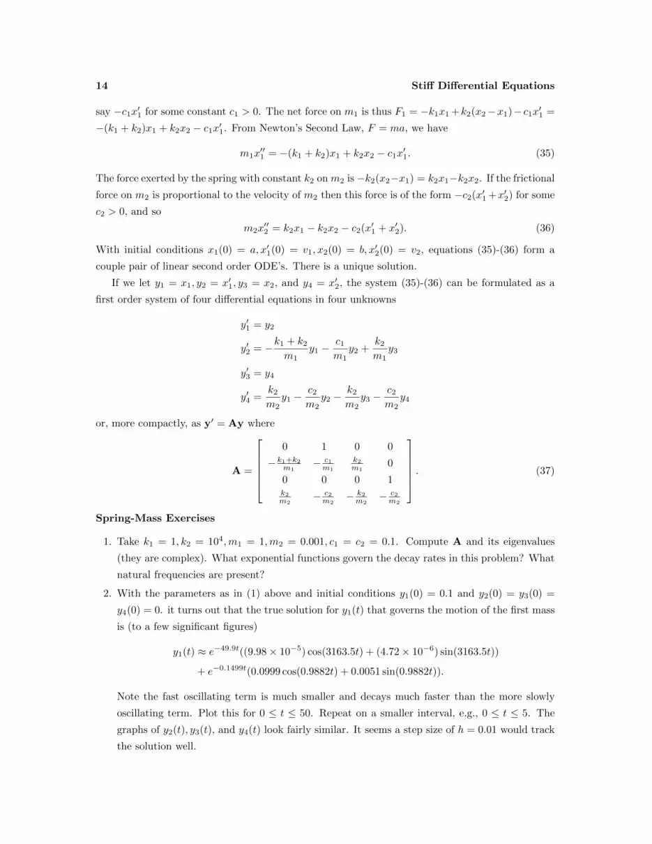
or, more compactly, as y′ = Ay where

A =

0 1 0 0

−k1+k2m1− c1m1

k2m1

0

0 0 0 1k2m2

− c2m2

− k2m2

− c2m2

. (37)

Spring-Mass Exercises

1. Take k1 = 1, k2 = 104,m1 = 1,m2 = 0.001, c1 = c2 = 0.1. Compute A and its eigenvalues

(they are complex). What exponential functions govern the decay rates in this problem? What

natural frequencies are present?

2. With the parameters as in (1) above and initial conditions y1(0) = 0.1 and y2(0) = y3(0) =

y4(0) = 0. it turns out that the true solution for y1(t) that governs the motion of the first mass

is (to a few significant figures)

y1(t) ≈ e−49.9t((9.98× 10−5) cos(3163.5t) + (4.72× 10−6) sin(3163.5t))

+ e−0.1499t(0.0999 cos(0.9882t) + 0.0051 sin(0.9882t)).

Note the fast oscillating term is much smaller and decays much faster than the more slowly

oscillating term. Plot this for 0 ≤ t ≤ 50. Repeat on a smaller interval, e.g., 0 ≤ t ≤ 5. The

graphs of y2(t), y3(t), and y4(t) look fairly similar. It seems a step size of h = 0.01 would track

the solution well.


3. Solve the system with Euler’s method and h = 0.01 out to time t = 5, or however far it will go.

Is it stable?

4. Repeat with the Implicit Euler method. Is the numerical solution stable? Accurate?

5. Repeat the last question with the Trapezoidal Method (23).

REFERENCES

[1] Butcher, J.C., 2016. Numerical Methods for Ordinary Differential Equations, Third Edition.

New York; John Wiley & Sons, Inc.

Documents

SIMIODE - STUDENT VERSION Stiff Differential Equations