BzzOde: a new C++ class for the solution of stiff and non-stiff ordinary differential equation systems

*Author to whom all correspondence should be addressed.

Computers Chem. Engng Vol. 22, No. 11, pp. 1595—1621, 1998( 1998 Elsevier Science Ltd

All rights reserved. Printed in Great BritainPII: S0098-1354(98)00233-6 0098—1354/98 $ — see front matter

BzzOde: a new C11 class for the solution of stiffand non-stiff ordinary differential equation systems

Guido Buzzi Ferraris and Davide Manca*

Department of Chemical Engineering ‘‘G. Natta’’, Polytechnic of Milan, Italy

(Received 8 March 1996; revised 16 March 1998)

Abstract

A new code for the solution of ordinary differential equation (ODE) systems was developed in C##

language. Three main aspects were studied: robustness, efficiency and ease of use. BzzOde is a new C## classintended to solve both stiff and non-stiff ODE problems numerically. Neither FORTRAN 77 nor Fortran 90was adopted as the reference language. C## was chosen in order to increase the implementation efficiencyand the ease of use and consistency features of the library. Although BzzOde is intended to solve both stiff andnon-stiff problems, this paper will only deal with stiff problems since they are the most interesting andcommonly occurring ones in everyday chemical problem solving. Several examples taken from both theliterature and real life cases, such as chemical kinetics problems, were investigated by comparing the BzzOdeperformances with state of the art Fortran ODE solvers. The paper describes the robustness feature andperformance of BzzOde applied not only to classical problems but also to specific tests that involve medium andlarge eigenvalue imaginary parts, discontinuous systems and problems with constrained integration variables.Medium-large ODE systems describing real life literature problems analyze and benchmark the efficiency of theODE solvers tested. New algorithmic techniques for identifying the discontinuity points, for working withconstrained variables and for increasing the Jacobian evaluation performance of a sparse ODE system areproposed and critically examined. A detailed description for the benchmark problems and correspondingresults is reported in appendixes A and B. ( 1998 Elsevier Science Ltd. All rights reserved.

1. Introduction

The state of the art Fortran ODE solvers adoptedfor the testing are: VODE (Brown et al., 1989),LSODE (Hindmarsh, 1980) DASPK (Brown et al.,1992) and IVPAG (IMSL 1995). DASPK, which iscapable of solving more general DAE systems, wasused for the ODE subset only. During the testing, theDASPK built in direct linear solver, which can factoreither dense or banded matrices, was adopted. TheDASPK preconditioned Krylov projection methodwas not used.

VODE, LSODE and DASPK are written in FOR-TRAN 77, whilst IVPAG is written in Fortran 90exploiting the dynamic memory allocation for theinternal working arrays.

We did not cover any test with CVODE that is theC language version of VODE and VODEPK since itdoes not seem to introduce new issues and features inthe ODE solver field. Only one problem (XIX) would

have exploited the sparse iterative linear solver featureof VODEPK and CVODE by means of the Krylovmethod but we chose not to implement any precon-ditioning matrix and to keep the comparison on thedirect linear solver side. As it will be shown later thisapproach results to be neither faulty nor incomplete.

Moreover we chose not to consider commercialpackages such as Speedup, Mathematica or Matlabsince we want to allow the user the freedom to buildup a program independently of both the packageinterface and of the macro language of those propri-etary programs. Moreover, as such packages areall purpose numerical solvers, they seldom achievethe performance features of the Fortran and C##

libraries specifically developed and fine-tuned for thesolution of the ODE systems. Finally, after severalbenchmarks, we have decided not to consider theFortran Numerical Recipes routines (Press et al.,1989) due to their poor performance. All the numer-ical benchmarks were performed on a personal com-puter (Pentium 150 MHz) under a multithreaded 32bit operating system, using double precision variablesand functions (REAL*8, double).

1595

The C## libraries and the C## test sourcecodes are available as freeware software (seeAppendix C).

2. Organization of the work

The following presentation will be divided into fourdistinct sections which will attempt to classify thewhole set of literature and real life problems withrespect to different problematics and characteristics:classical problems, robustness, efficiency and easeof use.

The set of correlated problems will be defined anddescribed for each section; each problem will be thendiscussed and tested with the four Fortran packages:LSODE, VODE DASPK and IVPAG and the C##

class: BzzOde. It is worth underlining that the wholeset of ODE systems belongs to the stiff problems class.Such problems test the reliability, robustness and effi-ciency of the ODE solvers to a higher extent.

In this paper the following pragmatic definitionof ‘‘stiff problem’’ is being used. A differential equa-tion and more generally an ODE system are stiff ifwhen integrated by means of a classic ODE solver(such as a Runge—Kutta IV order method orRunge—Kutta—Fehlberg method with error control)they go under a crisis situation. The same systemsonce integrated by means of a specifically geared stiffsolver do not show remarkable difficulties.

Given the vectors of n%2

components: y@, y, f, themulti-value methods adopted for the solution of thesystem:

y@"f (y, t), (1)

with the initial condition

y(t0)"y

0, (2)

embrace the following strategy (Radhakrishnan andHindmarsh, 1993).

The Nordsieck array is stored at point n:

zp"

hpy(p)

p!, p"0,2, P#1, (3)

where the method order is P, h"hn"t

n!t

n~1is the

stepsize and y"ynis the computed approximation of

y(tn) the exact solution at t

n. When the number of

variables is greater than one, each element of theNordsieck array is also an array of n

7elements. The

predictor action is evaluated at point n#1 throughthat array and it turns out to be

v"Dz, (4)

where D is the Pascal matrix. The Nordsieck array inn#1 is then calculated as

zp"v

p#r

pb, p"0,2 ,P#1, (5)

where b is evaluated through the solution of the fol-lowing non-linear system:

v1#b"hf (v

0#r

0b, t

n`1) (6)

which is solved by means of a Newton method.

The Backward Differentiation Formula (BDF) im-plemented in BzzOde is similar to those used inLSODE, i.e., fixed step, interpolated formulation. Thebenchmark case studies are reported in Appendix A interms of Fortran source code for each ODE system.Appendix B reports the total number of steps, func-tion evaluations, numerical Jacobian evaluations, LUdecompositions, absolute CPU time, final integrationtime and the absolute and relative integration toleran-ces for each problem and for each solver. Finally, eachsection of this paper reports at least two graphs. Thefirst shows the total CPU time with respect to a rela-tive scale where BzzOde is 1. The second correspondsto the number of function evaluations. Every bench-mark graph reports from left to right the bars corres-ponding to: BzzOde, VODE, DASPK, LSODE andIVPAG. An additional table follows the graphs andreports the relative and absolute CPU times andcorresponding function evaluations. The CPU timesrelating to the Classical Stiff Problems section havenot been reported since they are not measurable. Infact, each problem requires less than one hundredth ofsecond. As a consequence, the execution time becomescomparable with the time precision of the kernel anduser CPU routines reported by the operating system.In such cases, repeating each problem several times bymeasuring the mean CPU time is not enough, sincethe effective solution time becomes comparable withthe initialization procedures and it is also a functionof the total memory allocation and clean-up algo-rithms adopted during the test iterations.

3. Classical stiff problems

The first set of problems consists of systems witha limited number of equations and no discontinuities.These problems can be defined as classical stiff testsand are well known and widely used in literature forvalidation purposes. They present a severe test fornon-stiff packages. Nonetheless, all of the five stiffODE solvers tested here are able to integrate thesesystems without any great difficulty. Given the samerelative and absolute tolerances, the five algorithmssolved each problem with a comparable amount ofeffort. There is no clear difference in terms of solverefficiency. Since all of the five ODE solvers use thesame error control formula as proposed and describedby Hindmarsh (1980), it is clearly correct to adopt thesame relative and absolute tolerances. It is also evi-dent that this gives a consistent condition for thecomparison of all the ODE packages.

The performance of each package for this class ofproblems is measured by means of ‘‘function evalu-ations’’. This means the total number of times thedifferential equations system is called by the solverboth to perform the single steps towards the finalsolution and to evaluate the Jacobian matrix boundto the implicit nature of the multi-value method of theGear family. As previously mentioned, no CPU timesare reported for this class of problems. It is worth

1596 G.B. FERRARIS and D. MANCA

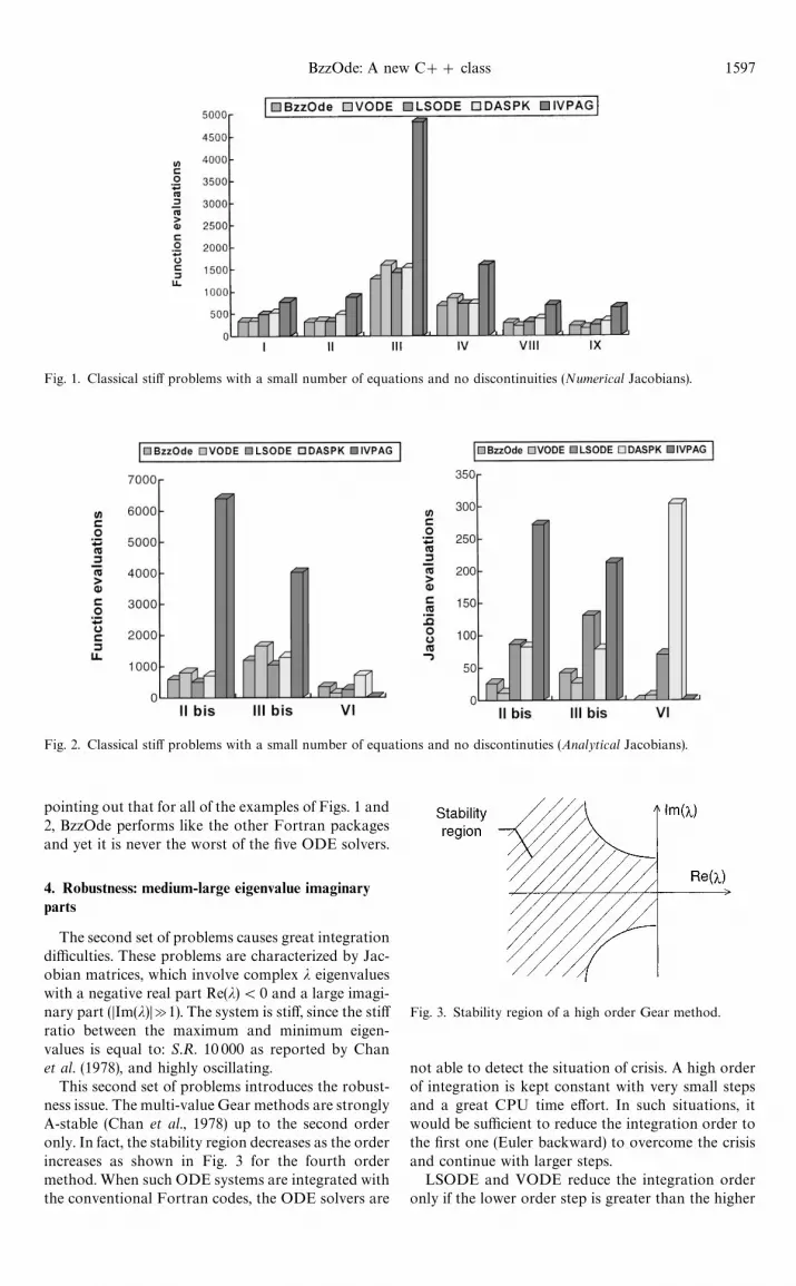
Fig. 1. Classical stiff problems with a small number of equations and no discontinuities (Numerical Jacobians).

Fig. 2. Classical stiff problems with a small number of equations and no discontinuties (Analytical Jacobians).

Fig. 3. Stability region of a high order Gear method.

pointing out that for all of the examples of Figs. 1 and2, BzzOde performs like the other Fortran packagesand yet it is never the worst of the five ODE solvers.

4. Robustness: medium-large eigenvalue imaginaryparts

The second set of problems causes great integrationdifficulties. These problems are characterized by Jac-obian matrices, which involve complex j eigenvalueswith a negative real part Re(j)(0 and a large imagi-nary part (DIm(j)DA1). The system is stiff, since the stiffratio between the maximum and minimum eigen-values is equal to: S.R. 10 000 as reported by Chanet al. (1978), and highly oscillating.

This second set of problems introduces the robust-ness issue. The multi-value Gear methods are stronglyA-stable (Chan et al., 1978) up to the second orderonly. In fact, the stability region decreases as the orderincreases as shown in Fig. 3 for the fourth ordermethod. When such ODE systems are integrated withthe conventional Fortran codes, the ODE solvers are

not able to detect the situation of crisis. A high orderof integration is kept constant with very small stepsand a great CPU time effort. In such situations, itwould be sufficient to reduce the integration order tothe first one (Euler backward) to overcome the crisisand continue with larger steps.

LSODE and VODE reduce the integration orderonly if the lower order step is greater than the higher

BzzOde: A new C## class 1597

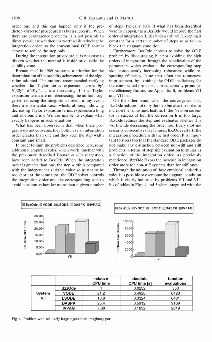
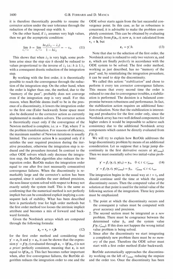
Fig. 4. Problem with relatively large eigenvalues imaginary part.

order one and this can happen only if the pre-dictor—corrector procedure has been successful. Whenthere are convergence problems, it is not possible todirectly evaluate whether it is worthwhile reducing theintegration order, so the conventional ODE solverschoose to reduce the step only.

During the integration procedure, it is not easy todiscern whether the method is inside or outside thestability zone.

Brenan et al. in 1989 proposed a criterion for thedetermination of the stability achievement of the algo-rithm adopted. The authors recommended verifyingwhether the Taylor series expansion terms: hy@,h2/2!yA, h3/3!y@A,2 are decreasing. If the Taylorexpansion terms are not decreasing, the authors sug-gested reducing the integration order. In any event,there are particular cases which, although showingdecreasing Taylor expansion terms, experience a longand obvious crisis. We are unable to explain whatexactly happens in such situations.

What has been observed is that, when these pro-grams do not converge, they both have an integrationorder greater than one and they keep the step widthconstant and small.

In order to limit the problems described here, someadditional empirical rules, which work together withthe previously described Brenan et al.’s suggestion,have been added to BzzOde. When the integrationorder is greater than one, the step width is comparedwith the independent variable value so as not to betoo short; at the same time, the ODE solver controlsthe integration order and the corresponding step toavoid constant values for more than a given number

of steps (typically 500). If what has been describedwere to happen, then BzzOde would impose the firstorder of integration (Euler backward) while keeping itconstant for a certain number of steps so as to un-block the stagnant condition.

Furthermore, BzzOde chooses to solve the ODEproblem by discouraging, but not avoiding, the highorders of integration through the penalization of theparameters which evaluate the corresponding stepsize, consequently increasing robustness while re-specting efficiency. Note that often the robustnessimprovement, by avoiding the ODE inefficiency forthe complicated problems, consequentially promotesthe efficiency feature, see Appendix B, problems VIIand VII bis.

On the other hand, when the convergence fails,BzzOde reduces not only the step but also the order toincrease the robustness feature. If the Newton correc-tor is successful but the correction b is too large,BzzOde reduces the step and evaluates whether it isworthwhile decreasing the order too. Every (not ne-cessarily consecutive) five failures, BzzOde restarts theintegration procedure with the first order. It is impor-tant to stress too that the standard ODE packages donot make any distinction between non-stiff and stiffproblems in terms of step size evaluation formulas asa function of the integration order. As previouslymentioned, BzzOde favors the increase in integrationorder more for non-stiff systems than for stiff ones.

Through the adoption of these empirical anti-crisisrules, it is possible to overcome the stagnant conditionwhich is clearly indicated by problems VII and VII-bis of tables in Figs. 4 and 5 when integrated with the


Fig. 5. Problem with decidedly large eigenvalue imaginary part.

Fig. 6. Predictor—corrector first order action across thediscontinuity.

Fortran packages: VODE, LSODE, DASPK and IV-PAG. In these two cases, BzzOde is clearly the handsdown winner in terms of performances with respect tothe other solvers. For problem VII-bis of Fig. 5, theeffective number of function calls performed byVODE, LSODE and IVPAG is more than 75 millioneach, so we have chosen to represent such integrationproblems as failed.

5. Robustness: large discontinuity problems

The third set of problems refers to ODE systemswith large discontinuity in the derivatives.

The main cause of the integration crisis for themulti-value methods when large discontinuities arepresent, is what we define as the ‘‘memory of the past’’.One of the strengths of the multi-value methods isthat they know what happened during the previoussteps and consequently tune the next step accordingto the integration history. While this is usually seena strength of these methods, it turns out to be a criticalflaw when the solver has to deal with the discontinuityitself. When it reaches the discontinuity point, theODE solver must discard the intrinsic ‘‘memory of thepast’’.

What has been said in terms of qualitative consider-ations will now be demonstrated through equations.For the sake of simplicity, let us now consider the firstorder method applied to the differential equation:y@"jy, with j suddenly changing value at a givenpoint t*, where h is the predictor step, b the correctionaction evaluated by the corrector and v the Nordsieckarray prediction at point n.

The corrector’s action becomes

v1#b"hjv

0#hjr

0b. (7)

Let us now suppose that the last predictor stepproposed by the ODE solver crosses the discontinuitypoint (see Fig. 6). As a consequence, in y

n~1we have

y@"jy whilst in ynwe have y@"j

2y. Therefore we get

b(1!hj2)"hj

2v0!hj

1v0

(8)

with r0"1 (for Euler backward method) and

v1"hj

1v0.

It can be finally deduced that

b"hv

0(j

2!j

1)

1!hj2

. (9)

Using such a formulation, it can be easily shownthat bP0 when hP0 since

limh?0

b"limh?0

hv0(j

2!j

1)

1!hj2

"0 (10)


it is therefore theoretically possible to resume thecorrector action under the user tolerance through thereduction of the imposed step width: h.

On the other hand, if j2

assumes very high values,then we get the asymptotic condition:

limj2?=

b" limj2?=

hv0(j

2!j

1)

1!hj2

"!v0. (11)

This shows that when j2

is very high, some prob-lems arise since the step size h should be reduced tovalues proportional to the inverse of j

2i.e.: h:1/j

2with a consequent drastic reduction of the integrationstep.

By working with the first order, it is theoreticallypossible to reach the convergence through the reduc-tion of the integration step. On the other hand, whenthe order is higher than one, the method, due to the‘‘memory of the past’’, probably does not convergeeven if the integration step is very small. For thisreason, when BzzOde deems itself to be in the pres-ence of a discontinuity, it lowers the integration orderto the first one (Euler backward). Some space mustalso be dedicated to the corrector action as currentlyimplemented in modern solvers. The corrector actionis theoretically exact only if the convergence of theNewton method is complete, i.e.: z"¹(z), where ¹ isthe problem transformation. For reasons of efficiency,the maximum number of Newton iterations is usuallylimited. The corrector action b is accepted only if itsatisfies the user required precision during the iter-ative procedure, otherwise the integration step is re-duced and the procedure iterated. In contrast to theother ODE solvers which only decrease the integra-tion step, the BzzOde algorithm also reduces the in-tegration order. BzzOde makes the integration orderequal to one after five (not necessarily consecutive)convergence failures. When the discontinuity is re-markably large and the corrector’s action has beenaccepted, since it satisfies the user defined precision,the non-linear system solved with respect to b may notexactly satisfy the system itself. This is the same asconfirming that the numerical method is not perfectlyimplicit but can be considered explicit implying a con-sequent lack of stability. What has been describedhere is particularly true for high order methods butthe first order method too looses the intrinsic implicitattribute and becomes a mix of forward and back-ward formula.

Given the Nordsieck arrays which are computedthrough the following formula:

zp"v

p#r

pb (12)

for the first order method and considering thaty@"z

1/h and y"z

0, it can be shown that the expres-

sion y@"f (y, t) evaluated through z1"hf (z

0, t) is not

a priori perfectly consistent, meaning that z1

is notequal to hf (z

0, t). This fact becomes rather important

when, after five convergence failures, the BzzOde al-gorithm reduces the integration order to one and the

ODE solver starts again from the last successful con-vergence point. In this case, as far as robustness isconcerned, it is advisable to make the problem com-pletely consistent. This can be obtained by evaluatingy@ directly from f (z

0, t); now z

1is not calculated from

v1#b, but

z1"y@/h. (13)

Note that due to the selection of the first order, theNordsieck array is reduced to only two vectors: z

0and

z1

which are finally perfectly in accordance with theODE system to be solved. The first order method,working as just described, has no ‘‘memory of thepast’’ and, by reinitializing the integration procedure,it can be used to skip the discontinuity.

We called this action: ‘‘stabilization’’ and chose toperform it every ten corrector convergence failures.This means that every second time the order isreduced to one due to convergence troubles, a stabiliz-ation is performed. The decision is a balanced com-promise between robustness and performance. In fact,the stabilization action requires an additional func-tion evaluation. Note that the stabilization is interest-ing and productive for the first order only, since theNordsieck array has two well defined components; forhigher orders it would be impossible to achieve suchconsistency due to the additional Nordsieck arraycomponents which cannot be directly evaluated fromf (y, t).

We will try to explain how BzzOde addresses thelarge discontinuity problem by means of an additionalconsideration. Let us suppose that a large jump dis-continuity in the first derivative occurs at y(t

+6.1).

Then we must essentially solve two initial-value prob-lems:

y@"f1

(y, t), y(t0)"y

0, 0)t)t~

+6.1, (14)

y@"f2

(y, t), y(t~+6.1

)"y0, t`

+6.1)t)t

065.

The integration begins in the usual way at t"t0

andshould continue until the time at which the jumpdiscontinuity occurs. Then the computed value of thesolution at that point is used for the initial value of thefollowing section of the integration. Three key pointsmust be emphasized:

1. The point at which the discontinuity occurs andthe consequent y values must be computed withgreat accuracy and precision.

2. The second section must be integrated as a newproblem. There must be congruence between thedetermined value y

0and the system value

f (y, t`+6.1

). If this does not happen the wrong initialvalue problem is being solved.

3. Since after the discontinuity we start integratinga completely new problem there must be no mem-ory of the past. Therefore the ODE solver muststart with a first order method (Euler backward).

BzzOde automatically approaches the discontinu-ity working on the left of t

+6.1, reducing the stepsize

and the order too. Once the discontinuity has been


Fig. 7. Problem with a large discontinuity.

numerically evaluated to the assigned user precision,BzzOde restarts all the integration procedure bymeans of equation (13), therefore respecting the ODEconsistency.

As can be seen in Fig. 7, BzzOde is the only solverable to go beyond the imposed discontinuity of prob-lem X. Note that the discontinuity point often is notknown a priori as in problem X, therefore it is notpossible to stop and then restart the integration pro-cedure across the discontinuity point.

6. Robustness: problems with constrained integrationvariables

The fourth set of problems refers to ODE systemswhich require constrained integration variables.

In many physical models but mainly in chemicalproblems, the solution vector, or part of it, mustbelong to an interval defined by lower and/or upperbounds. For example in the simulation of typicalreaction mechanisms involving chemical kineticschemes, the molar fractions, which are the integra-tion variables, must fall inside the range: 0,2 , 1. Theupper and lower limits for the integration variablescan either assume scalar or vector values.

Let us first look at the risks involved when noconstraints can be directly specified to the ODE sol-ver. We will refer to the chemical reaction simulationof kinetic schemes, typically oxidation and pyrolysis,assuming that the integration variables y

iare the

components’ molar fractions. If the user, directlymodifies the negative values of y

i, as passed by the

solver, within the system routine that describes theproblem, making them equal to zero, he is makinga highly dangerous move in terms of numerical con-sistency and the solver will almost certainly halt.

A second option, often adopted in order to main-tain the macroscopic numerical solver consistencyduring the integration path, is to choose the molarfractions as y variables and to work inside the systemroutine (FEX in LSODE and VODE notation) withderived variables: i.e. concentration vector c. Whencibecomes negative, it is possible to make c

i"0 in

order to avoid possible floating point run time errorssuch as logarithms or square roots of negative values.Doing this also formally introduces a more subtleissue: the function f (y, t) of equation (1) can becomelargely discontinuous and run into consequent integ-ration problems due to the user’s manipulation of theauxiliary variables: c. On the other hand, the usercould choose neither to modify y nor to correct thederived c array. However, by accepting the negativevalues proposed by the ODE solver for the elementsof y, some derived quantities can loose physical signif-icance with the occurrence of numerical problems. Ifwe consider the conversion of a specific reactantdefined as

g"y(0)!y(t)

y(0)(15)


Fig. 9. Possible numerical solution of the differentialequation: y@"!y2.

Fig. 8. The analytical solution of the differential equation:y@"!y2.

when y(t) becomes negative g is greater than 1, i.e.a conversion higher than 100% is apparentlyachieved. This fact is also dangerous when consider-ing elementary direct reactions of the form: R

1"lc

icj

because when ci(0 or c

j(0NR

1(0, the reactants

are produced instead of being consumed and, ratherthan increasing, the products are then subtractedfrom the reacting environment with total loss ofmodel significance. The decision to correct neithervector y nor c would clearly lead to a math errorwhenever a reaction of the form: R

2"lc0.5

iwas pres-

ent. The reaction: R3"!lc2

iwould also be very

problematic. At first glance, the reader might thinkthat there would be no problem whatever c

iwere,

because ciis squared before being multiplied by !l.

In any case by considering the analytical solution ofthe differential equation: y@"!y2 as shown in Fig. 8where y approaches the asymptote 0`, it can beshown that as soon as y gets any small negative value,the procedure becomes unexpectedly divergent dueto a fortuitous numerical approximation proposedby the ODE solver, and so yP!R as shown inFig. 9.

To avoid the problematic divergence due to theR

3structure, the user could choose to decrease the

numerical tolerance in order to increase the numericalaccuracy, reducing at the same time the maximumstep size allowed, so to control the solver behaviorwhen getting closer to y"0. This action, aimed atincreasing the algorithm robustness, would simulta-neously reduce the solver efficiency. In fact, while theODE procedure could noticeably increase the integra-

tion step due to the final differential equation relax-ation near the asymptote y"0, the user wouldactually limit the maximum integration step andstress the numerical accuracy in order to avoid anynegative value of y with a consequent diverging be-havior.

Previous considerations have shown that the cor-rect approach to upper and/or lower constraint valuesfor the integration variables is to leave the task ofdealing such quantities to the ODE solver. VODEand LSODE do not allow the user to specify anyupper and/or lower bound for the solution vector.DASPK apparently allows a non-negative definitionof the solution vector throughout the integration pro-cedure.

By setting the internal DASPK indexINFO(10)"1 the user can specify that the y vectormust be non-negative. In a certain sense, this option isthe first step towards the full vector minimum andmaximum constraints feature. In any case, if themodel subroutine (RES in DASPK notation) doescontain functions which cannot take negative argu-ments then the integration program will abort duringthe execution with a floating point exception as soonas y becomes negative. This could seem to be nonsen-sical since DASPK has been informed that negativey elements are not allowed. The problem lies in theODE solver action on the y definition. DASPKchecks that no negative values have been evaluatedand makes the negative elements of y equal to zeroonly after the corrector procedure has reached theconvergence within the required precision limit. Thismeans that if, during the predictor step or the correc-tor iterations, any value of y becomes negative thesolver will not take any action and the system proced-ure (RES) will be called without advice. This is thereason for the possible math error described pre-viously.

The DASPK solver also relies on another methodto deal with this problematic: the user can tell theODE solver that a non-valid y vector has been passedto the RES routine, by setting the communicationstatus variable IRES"1 and immediately returningthe control to the solver. In this case, DASPK reducesthe step size and re-attempts the convergence withinthe corrector, but if the integration routine at the lastsuccessful step n has found yn

i"0 and y@(n)

i(0 then

any predictor action on the following n#1 step is asfollows: yn`1

i,13%$*#503(0 and DASPK goes on reducing

the step size indefinitely, still proposing yn`1i,13%$*#503

(0,until DASPK finally fails the integration proceduredue to a step size hP0.

As previously stated, the correct approach to theconstraints problem must come from the ODE solverin terms of decisions to be made at each step of theintegration procedure. This is the only way in whichthe ODE system routine is safe and the math errorsare a priori avoided within it. Once an ODE objectof the BzzOde class has been defined, the user cansimply assign the maximum and minimum constraints


Fig. 10. Problems which request constrained integration variables.

vectors through two functions:

BzzOde o; // the BzzOde object is defined hereBzzVectorDouble yMax(n); // the two bound vectorsBzzVectorDouble yMax(n); // are defined here// TO DO: Initialization of yMin and yMax goes here2o.SetMaxConstraints( & yMax); // Assignment of theo.SetMinConstraints( & yMin); // constraints yMin and yMax

The solver automatically handles the constraintstaking care not to violate the assigned bounds. Thecontrol is performed before passing any illegal valueto the ODE system routine.

The strategy adopted by BzzOde to handle theconstrained problem is the following:

The correction b to the predicted solution value, isapplied to both the terms: v

0and v

1and so to solve the

non-linear system (6) and to have the term v0#r

0b

(i.e. y) satisfying the constraints.If the Newton-like nonlinear solver does not con-

verge within the user assigned precision the stepsize

and the order are reduced. In this way the correctionb is accepted only when the nonlinear system (6)is solved accurately within the assigned precisionand at the same time y belongs to the bounds’ interval.The order reduction is conceived to increase the stab-ility of the method and to loose the memory of thepast.

It is fundamental to underline that working in thisway the function system is always called with safey values that satisfy the assigned constraints. For thisreason, BzzOde is the only routine able to solve prob-lems XII, XIII and XIV (see Fig. 10).


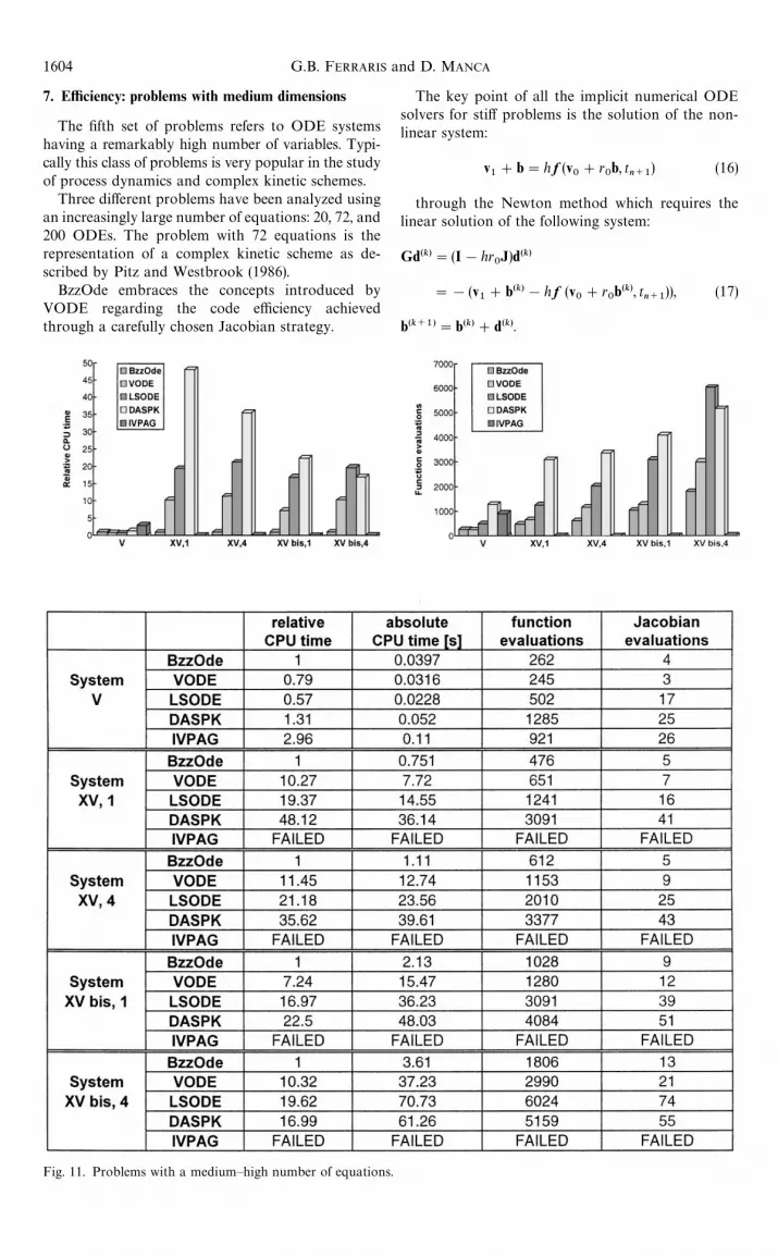
Fig. 11. Problems with a medium—high number of equations.

7. Efficiency: problems with medium dimensions

The fifth set of problems refers to ODE systemshaving a remarkably high number of variables. Typi-cally this class of problems is very popular in the studyof process dynamics and complex kinetic schemes.

Three different problems have been analyzed usingan increasingly large number of equations: 20, 72, and200 ODEs. The problem with 72 equations is therepresentation of a complex kinetic scheme as de-scribed by Pitz and Westbrook (1986).

BzzOde embraces the concepts introduced byVODE regarding the code efficiency achievedthrough a carefully chosen Jacobian strategy.

The key point of all the implicit numerical ODEsolvers for stiff problems is the solution of the non-linear system:

v1#b"h f (v

0#r

0b, t

n`1) (16)

through the Newton method which requires thelinear solution of the following system:

Gd(k)"(I!hr0J)d(k)

"!(v1#b(k)!h f (v

0#r

0b(k), t

n`1)), (17)

b(k`1)"b(k)#d(k).


Fig. 12. Problems with a medium—high number of equations.

Most of the ODE chemical engineering problemshave the following characteristics:

f each function evaluation is highly time consuming,f the Jacobian matrix J is evaluated numerically (fi-

nite difference),f the number of equations is quite high.

From this point of view, it is clear that the functionevaluations have the greatest impact on the CPUtime. As the number of system equations is increased,the Jacobian evaluation becomes more and moreexacting.

In the first obsolete ODE programs which weretuned for a small number of equations, the Jacobianmatrix was evaluated and factored at each step inorder to calculate the correction vector: b.

LSODE and DASPK keep the matrix G constantfor some steps to avoid the evaluation of the JacobianJ and the G factorization at each step.

VODE, IVPAG and BzzOde introduce a furtherefficiency improvement. The Jacobian J is stored sep-arately from matrix G so that J does not have to beevaluated whenever matrix G must be re-factored. Asa matter of fact, G is updated when there is a step sizechange (h) or an integration order switch (r

0). By

working in this way, it is possible to keep J constantfor a higher number of steps. Since the Jacobiannumerical evaluation usually requires n

%2system

f evaluations, the great advantage of VODE andBzzOde over LSODE and DASPK becomes evident.This is clearly demonstrated in Fig. 11 where BzzOdeand VODE behave in an almost completely oppositemanner to LSODE and DASPK which, by perform-ing more Jacobian evaluations, greatly increase thetotal function calls and, therefore, the CPU time.IVPAG, on the contrary, is not able to reach thesolution. It is worth pointing out the clear paral-lelism between function calls and Jacobian evalu-ations which can be seen by comparing Figs. 11and 12.

BzzOde follows a different criterion with respect toVODE in determining when to update the Jacobianmatrix. The first significant difference is that BzzOdechecks whether J is out of date through the followingequation:

y@n`1

:y@n#J ) (y

n`1!y

n)#f

t) (t

n`1!t

n), (18)

where y@n`1

, y@n, y

n`1, y

nare the variables at the n and

n#1 iteration, J is the stored Jacobian matrix and ft

the ODE system time derivative.When the equations number n

%2is high the Jac-

obian numerical evaluation is rather time consumingso it is advisable not to update matrix J very often.Conversely, if the system is very simple, it is advisableto evaluate the Jacobian matrix more frequently inorder to increase the Newton method efficiency withvery little extra effort. Due to these considerations, wedecided to evaluate a new Jacobian matrix at mostafter m steps, with m a function of n

%2:

m"min(20#5(n%2!3), 50). (19)

If by doing so n%2*9, then m reaches the maximum

allowed value: 50. At the same time when n%2"2, then

m becomes 15 because in this case the Jacobian up-date is not time consuming.

Since the Jacobian consistency is controlled ina deeper and more accurate way with respect to theconventional ODE routines, it is also safer to increasethe maximum allowed steps performed by keeping theJacobian matrix constant. As a matter of fact, VODEand LSODE perform the Jacobian evaluation at leastevery 20 steps, while BzzOde allows the Jacobianmatrix to be kept constant for a maximum of 50 steps(when n

%2*9) with a further performance improve-

ment. It is worth adding that the introduction ofBroyden and Barnes’s correlation with the aim ofefficiently updating the Jacobian matrix and conse-quently delaying the direct evaluation, did not giveinteresting results, so it was abandoned.


Fig. 13. Problems with a high number of equations.

8. Efficiency: problems of large dimensions

For the problems comprising a high number ofdifferential equations BzzOde adopts two main fea-tures which allow solution efficiency to be greatlyincreased (Fig. 13). The improvement is achievedthrough the optimization of the Jacobian matrixevaluation and the development of specificallytailored numerical algorithms for the solution of thelinear system.

The former feature works on the reduction of func-tion evaluations through an efficient handling of theJacobian matrix. The latter feature optimizes the fac-torization of the linear system matrix: (I!hr

0J).

When profiling the execution time using the latestcompilers, it often happens that an impressive80—90% of the CPU time is spent on the functionevaluations. The remaining 10—20% goes for the LUfactorization and the step evaluation performed bythe ODE solver. That is why BzzOde VODE andIVPAG are more efficient than LSODE and DASPKin this case (Byrne and Dean, 1993).

The lower number of Jacobian evaluations is themain reason for the total CPU time reduction. In fact,n%2

being the number of differential equations, eachJacobian evaluation usually requires n

%2function

calls. Therefore the total number of function evalu-ations n

&%can be approximated by the following


Fig. 14. Boolean presence array of a Jacobian matrix. Fig. 15. Banded Jacobian matrix with off-diagonal elements.

expression: n&%:(n

J%) n

%2)#n

45%1where n

J%is the

number of Jacobian evaluations and n45%1

the numberof integration steps.

In the previous expression, the former term (nJ%) n

%2)

is dominant when considering large ODE systems.Once again, IVPAG does not achieve good results interms of CPU time due to an anomalous value of theJacobian evaluations. The Jacobian structure isa function of the problem scheme itself. The Jacobianmatrix J"Lf/Lx is numerically evaluated by theODE solver if not otherwise supplied by the user. Itcan be observed that not all of the equations arealways function of all of the unknowns. Therefore, theJacobian matrix can be evaluated by modifying all ofthe non-interacting variables at the same time (Curtiset al., 1974). In fact, let us now consider the followingstructure of the Jacobian matrix (Fig. 14): where the (z)symbol indicates the direct functional bound betweenthe x

jvariable and the f

ifunction.

In this example, it is possible to increment:Mx

1, x

2, x

3N first, then Mx

4, x

5N at the same time. In this

way, the J evaluation requires only two calls to theODE system f instead of the original five calls. Theincreasing sparsity of the Jacobian matrix accountsfor the decrease in the number of groups and also forthe total CPU time reduction. It is evident from whathas been said previously that it is necessary to knowa priori the Boolean presence array of the Jacobianmatrix in order to identify the groups and then im-prove the ODE solver efficiency. It is therefore pos-sible to identify n

'variable groups through a prior

analysis of the Boolean presence array. When work-ing with sparse matrices, n

'is usually a fraction of

n%2

so the total number of function evaluations can beapproximated by n

&%:(n

J%) n

')#n

45%1. The CPU time

saving is therefore evident and remarkable. Givena generic sparse matrix, none of the Fortran solvers isable to exploit the intrinsic structure of the Jacobianmatrix for identifying the suitable groups. BzzOde, onthe contrary, determines the grouping strategy whenthe user supplies the Boolean presence array of theJacobian matrix.

A different approach is adopted by classical ODEsolvers, however, when the Jacobian is a bandedmatrix with total band width: n

"where n

"(n

%2. In

such cases, VODE, LSODE, DASPK and IVPAGmake use of this knowledge to evaluate the J matrix

thus reducing the function calls number from n%2

to n".

For example, if the differential equation system istridiagonal then only three function evaluations willbe necessary to store J independent of the total num-ber of equations: n

%2. BzzOde improves at a further

extent what has been said. If the system matrix isbanded, it does not mean it is necessarily dense insidethe band itself. Often it is necessary to increase theband width to a great extent in order to take intoaccount only a small number of elements which lie faroff the diagonal, describing the interactions betweennon-adjacent equations. For example, this problemarises when modeling control loops, pumparounds,overflashes and interconnections for distillation col-umns. Such off-diagonal elements greatly increase theband width whilst leaving the total banded matrixalmost empty (Fig. 15).

In such cases, the classical ODE solvers must great-ly increase the number of function evaluations for theJacobian calculation since n

"is very high. BzzOde

instead is still able to identify the small number ofequations which are responsible for the band widthincrease. Given the Boolean presence matrix, BzzOdedetermines the n

'groups with n

'@n

". The consequent

CPU time saving can be dramatic.When large ODE systems are involved, BzzOde

changes the criterion about the maximum number ofsteps after which the Jacobian matrix must be up-dated. Condition (19) is replaced by a quantity that isa function of the CPU time required both to evaluateJ and to factor it. Figure 16 shows a problem withbanded Jacobian matrix.

Since the system’s dimensions are greater, it is nowpossible to accurately measure the CPU times and toquantify at runtime the effective weight of the functionevaluations needed to load J and of the linear systemsolver subject to the (I!hr

0J) factorization.

It is important to stress the fact that the Jacobianloading procedure is basically a function of n

'not of


Fig. 16. Problem with banded Jacobian matrix.

Fig. 17. The Boolean presence array for Problem XVIII.

n%2

. Moreover, if BzzOde realizes that the (I!hr0J)

factorization is CPU intensive, it may keep the stepwidth constant also when it would be possible toincrease it. This decision increases the number of stepsbut at the same time avoids any further factorizationrequired by a step width change.

Figure 17 shows the Boolean presence matrix ofa system describing the dynamic integration of anunsteady-state heterogeneous catalytic reactor asdescribed in literature by Boreskov and Matros in1983. For the sake of simplicity, the number of ODEequations has been reduced to 124 in order to graphi-cally represent the Jacobian matrix structure.

The performance comparison between BzzOde andVODE is possible and viable since both the ODEsolvers use a banded factorization routine.

As aforementioned the Jacobian matrix is updatedless frequently than VODE, since the problem dimen-sion is large.

The total band width is 17 (8 left diagonals, 8 rightdiagonals, 1 main diagonal) and therefore the classicalFortran routine: VODE calls the function routine 17times in order to evaluate J. However, BzzOde, hav-ing analyzed the Boolean presence matrix, is able toidentify 5 separate variable groups reducing thematrix J evaluation to only 5 function calls. The CPUtime saving can be even more dramatic when thisoperation is applied to real life problems of greaterdimensions and band widths.

The last problem proposed is represented by systemXIX which sums up all of the previously mentionedcharacteristics.

Despite the sparse problem structure that wouldsuggest the adoption of VODEPK as a specificallydeveloped Fortran routine, we intentionally keep onworking with the standard VODE solver. VODEPKis the recommended ODE solver when sparse systemsare involved. Such routine implements the iterativeKrylov linear solver based on a preconditioningmatrix and a scaling technique.

BzzOde on the contrary does not implement a lin-ear iterative solver but addresses this topic by meansof a direct method that analyzes the sparse matrixstructure and reorganizes it so to minimize the mem-ory allocation and the number of operations. A directCPU time comparison between BzzOde and VODE istherefore at first sight not possible. It is nonetheless


Fig. 18. The Jacobian matrix structure of problem XIXwhere N"1000.

viable to compare the total number of functioncalls.

The Jacobian matrix of problem XIX is highlysparse and its dimensions are considerable(1000]1000).

Through the Boolean presence matrix (Fig. 18),BzzOde is able to identify three variable groups(n

'"3). This means that the Jacobian evaluation

does not take 1000 function calls. Just three functioncalls are sufficient. Lastly, the LU factorization isperformed by BzzOde on the generic sparse matrixwhich, because of its structure, cannot be considereda banded array. Once again the linear C## systemsolution exploits the J structure by working with theexisting elements only.

Let us now consider the CPU times. One couldargue that the great CPU time required by VODE isdue to the inappropriate factorization of the densematrix. This is not true. We have substituted inBzzOde the linear sparse solver with a general pur-pose Gauss dense LU decomposition routine, puttingthe comparison between BzzOde and VODE on thesame level. The CPU time of BzzOde increases from67.5 s (sparse linear solver) to 219.6 s (Gauss denselinear solver), on the contrary VODE requires2632.9 s to solve the same problem. Once put on thesame level: BzzOde takes less than 4 min compared tomore than 43 min working with VODE.

Therefore the great BzzOde performance improve-ment with respect to VODE can be summarized inthree points:

1. Each Jacobian evaluation requires only three func-tion calls as opposite to VODE that calls system (1)1000 times.

2. The Jacobian evaluations are very low since theproblem is of large dimensions. This is achieved bymeans of two stratagems that characterize BzzOde.

The need for the Jacobian update is controlledthrough equation (18). The Jacobian matrix isevaluated as less frequently as possible since theproblem is of large dimensions.

3. When using the dense matrix factorization,BzzOde realizes that it is heavier than the corres-ponding sparse matrix solver. As a consequence itdecreases the number of factorizations from 66 to50 by means of keeping the step width more con-stant. The total number of steps increases but thetotal CPU time is at the same time optimized.

As previously mentioned, these data are not meantto be a comprehensive comparison between BzzOdeand VODE (Fig. 19). On the contrary, we wish tounderline the particular aspects and features ofC## with respect to Fortran by stressing the greatease of use of a programming language of this typeand the reduced requirements in terms of hardwareand CPU time when dealing with specific real life,large dimension problems.

Another very important factor in the higher effi-ciency is its being based on the optimization of thelinear system solution which works on the factoriz-ation of the matrix (I!hr

0J). Thanks to the ability of

C## to recognize the matrix structure of the linearsystem easily and to the dynamic memory allocationof the strictly necessary space for the matrix itself, it ispossible to deploy several factorization alternativeswhich would be very difficult or even impossible todevelop in Fortran.

For example: if a matrix cannot be convenientlystored as a banded matrix due to its sparsity, then itwill be dealt as a sparse matrix with a memory alloca-tion equivalent to the non-zero elements only. In thiscase, the C## dynamic memory allocation willcreate and destroy each necessary matrix coefficientduring the sparse matrix factorization leading toa real-time minimal memory requirement and conse-quent minimal CPU effort.

9. Why C11?

C## was chosen for the implementation ofBzzOde and, more generally, of BzzMath, the numer-ical analysis library to which BzzOde belongs, sincethis language allows safer code to be written efficient-ly. This code is easier to use than Fortran mainlybecause of the intrinsic nature of C## which isbased on the object oriented approach. Some charac-teristics which distinguish the BzzOde class fromthe common ODE Fortran subroutines are describedbelow.

Where VODE, LSODE and DASPK are con-cerned, the user has to provide the subroutines withtwo working vectors (typically the real vector:RWORK and the integer one: IWORK) which arenecessary for the routines to store all the internalvariables such as the Jacobian matrix and the pivot-ing index array for the LU factorization. The IVPAG


Fig. 19.

routine which is developed in Fortran 90 with thedynamic memory allocation feature has a neater userinterface compared to the conventional FORTRAN77 packages.

The object oriented approach of C## does notrequire the user to specify the internal use work ar-rays. In fact, the object deals them automatically,dynamically allocating and freeing up the necessarymemory: the data are inside the object and thereforemasked (Manca and Buzzi-Ferraris, 1995b). Thanksto the data masking, the user cannot inadvertentlyviolate any important variable. As an example: if theuser modifies any working vector element between thecalls to the Fortran ODE solver, then unpredictableerrors may occur.

When the C## object is defined, it is automati-cally initialized. It is therefore unnecessary to call theODE subroutine a first time with a special index inorder to initialize a new problem and consequentlymodify the same index (ISTATE) for any subsequentcall. The object knows all its history and then actsaccordingly.

Another great feature of the C## language is themultiple instance characteristics. By this we mean thatthere can be several BzzOde objects at the same time,each working on the integration of a distinct problem:there is no need, as happens in Fortran, to save theworking data arrays alternatively before switchingbetween problems.

As previously mentioned, the dynamic memorystorage automatically allocates and frees up the re-

quested object’s RAM. As soon as the object movesout of scope, the allocated memory is freed up. There-fore there is no need to over-dimension the internalworking array in order to solve different problems orto overlap the vectors in order to save space and solvelarger ODE systems.

All of these characteristics not only improve theuser-friendliness of the BzzOde class for less familiarusers but, also to a certain extent, the coding efficiencyand clarity for the advanced programmer who imple-ments the numerical C## classes.

10. Conclusions

A new C## class: BzzOde for the solution ofODE systems was implemented. The authors basedall of the development work on two main features:robustness and ease of use. Thanks to the CPU powerof modern computers, the authors feel that the mostimportant feature required of any ODE solver is theability to reach the solution regardless of the effortmade.

At the same time, however, the improvement inrobustness is often synergetic with the efficiency fea-ture. This could, at first sight, seem incorrect andinconsistent. Nonetheless, the improvement in robust-ness often allows the solver to avoid typical crisissituations and reach the solution through a morestable and therefore efficient path. The results shownin this paper demonstrate that BzzOde performance isbetter than common Fortran ODE solver ones.


In conclusion, the BzzOde ease of use was achievedthrough a globally revised object oriented approachin C##.

Acknowledgements

The authors acknowledge Prof. E. Ranzi for hisuseful suggestions and the reviewers for their preciousconsiderations, annotations and suggestions.

Nomenclature

b corrector array for the Nordsieck arrayc concentration vector for a given kinetics

problemD Pascal matrixd Newton method correction for vector bf vector-valued functionft

time derivative of the vector-valued functionG Jacobian of the Newton methodh integration step proposed by the predictorI identity matrixIm( ) imaginary partJ Jacobian arraym maximum number of steps after which a new

matrix J has to be evaluatedn nth stepn"

total band width for the banded matrixn%2

total number of equationsn&%

total number of function evaluationsn'

number of variable groups in which matrixJ can be logically divided

nJ%

total number of Jacobian evaluationsn45%1

total number of stepsn7

total number of integration variablesp pth order of the methodP order of the methodR reaction rateRe ( ) real partrp

corrector coefficient for the Nordsieck arrayS.R. stiff ratio¹ problem transformationt* discontinuity pointt independent integration variablev prediction of the Nordsieck arrayy dependent integration variables arrayy molar fractions vectory@ first derivative vectoryA second derivative vectory@A third derivative vectory(p) pth derivative vectorz Nordsieck array

Greek letters

g reactant conversionj Jacobian eigenvaluel stoichiometric array

Subscripts and superscripts

b bandeq equation

fe function evaluationsg groupi ith componentj jth componentJe Jacobian evaluationsjump discontinuity point in the y valuesn nth componentout final value for the independent integration

variablep pth integration orderstep steps performedt time derivative

Symbols

z element presence inside the Boolean pres-ence array

L partial derivativeD D absolute valueE E vector norm

References

Boreskov, G.K. and Matros, Y.S. (1983) Unsteady-state per-formance of heterogeneous catalytic reactions. Catal.Rev. Sci. Engng. 25, 551—590.

Brenan, K.E., Campbell, S.L. and Petzold, L.R. (1989) Nu-merical Solution of Initial-»alue Problems in Differen-tial-Algebraic Equations. North-Holland, New York.

Brown, P.N., Byrne, G.D. and Hindmarsh, A.C. (1989)VODE: a variable coefficient ODE solver. Siam J. Sci.Statist. Comput. 10, 1038—1051.

Brown, P.N., Hindmarsh, A.C. and Petzold, L.R. (1992)A Description of DASPK: A Solver for ¸arge-Scale Dif-ferential-Algebraic Systems. Lawrence Livermore Na-tional Report, UCRL.

Byrne, G. and Dean, A.M. (1993) The numerical solution ofsome kinetics models with VODE and CHEMKIN II.Comput. Chem. 17, 297—302.

Chan, Y.N.I., Birnbaum, I. and Lapidus, L. (1978) Solutionof Stiff Differential Equations and the Use of ImbeddingTechniques. Ind. Engng. Chem. Fundam. 17, 133—149.

Cohen, S.D. and Hindmarsh, A.C. (1994) CVODE UserGuide. ¸awrence ¸ivermore National ¸aboratory Re-port ºCR¸-MA-118618.

Curtis, A.R., Powell, M.J.D. and Reid, J.K. (1974) On theestimation of sparse Jacobian matrices. J. Inst. Maths.Appl. 13, 117—120.

Ehle, B.L. (1974) A comparison of numerical methods forsolving certain stiff ODE, Victoria University, Rep. 70.

IMSL (1995) IMSL Math Library, ºser Manual.Hindmarsh, A.C. (1980) LSODE and LSODI, Two new

initial value ordinary differential equation solvers.ACM SIGNºM Newslett. 15, 10—11.

Manca, D., Faravelli, T., Pennati, G., Buzzi Ferraris G. andRanzi, E. (1995a) Numerical integration of large kineticsystem. ICheaP-2 Conf. Ser. ERIS. 115—121.

Manca, D. and Buzzi Ferraris, G. (1995b) Objects are notODEs: ¼hy it is worth quitting fortran to enter C##.ICheaP-2 Conf. Ser., ERIS, 85—94.

Petzold, L. (1983) Automatic selection of methods for solvingstiff and non-stiff systems of ordinary differential equa-tions. SIAM J. Sci. Statist. Comput. 4, 136—148.


Pitz, W.J. and Westbrook, C.K. (1986) Chemical kinetics ofthe high pressure oxidation of n-butane and its relationto engine knock. Combust. Flame 63, 113—133.

Press, W.H., Flannery, B.P., Teukolsky, S.A. and Vetterling,W.T. (1989) Numerical Recipes in Fortran. CambridgePress, Cambridge.

Ralston, A., Rabinovitz, P. (1988) A First Course in Numer-ical Analysis, McGraw-Hill, London.

Radhakrishnan, K. and Hindmarsh, A.C. (1993) Descriptionand use of LSODE, the Livermore Solver for OridinaryDifferential Equations. NASA Ref. Publ. 1327, Liver-more.

Sincovec, R.F., Erisman, A.M., Yip, E.L. and Epton, M.A.(1981) Analysis of descriptor systems using numeri-cal algorithms. IEEE ¹rans. Automat. Control, 26,139—147.

Appendix A. ODE Systems classification. The description language is FORTRAN

Notation: f(i) right-hand side of the ODE systempd(i,j) partial derivatives of the analytical Jacobian: Lf

i/Lx

jy(i) dependent integration variablesy0(i) initial conditions for t"0

(only the non-zero components are specified)t independent integration variableneq total number of ordinary differential equations

System I: Ozone Decomposition, Bowen et al. (1963) (numerical Jacobian)y0(1)"1.f(1)"!y(1)!y(1)*y(2)#3.D0*98.D0*y(2)f(2)"98.D0*(y(1)!y(1)*y(2)!3.D0*y(2))

System II: Chemical Kinetics, Robertson (1967) (numerical Jacobian)y0(1)"1.

r1"0.04D0*y(1)r2"1.D4*y(2)*y(3)r3"3.D7*y(2)*y(2)

f(1)"!r1# r2f(2)"r1! r2! r3f(3)"r3

System II bis: Chemical Kinetics, Robertson (1967) Classical variant (analytical Jacobian)y0(1)"1.

ODE systemr1"0.04D0*y(1)r2"1.D4*y(2)*y(3)r3"3.D7*y(2)*y(2)f(1)"!r1# r2f(2)"r1! r2! r3f(3)"r3

Jacobian matrixpd(1,1)"!.04D0pd(1,2)"1.D4*y(3)pd(1,3)"1.D4*y(2)pd(2,1)".04D0pd(2,2)"!1.D4*y(3)!6.D7*y(2)pd(2,3)"!1.D4*y(2)

pd(3,2)"6.D7*y(2)

System III: Belousov Reaction, Field and Noyes (1974) (numerical Jacobian)y0(1)"4.y0(2)"1.1y0(3)"4.

f(1)"77.27D0*(y(2) # y(1)*(1.D0! y(2)!8.375D-6*y(1)))f(2)"(!y(2)*(1.D0# y(1)) # y(3))/77.27D0f(3)".161D0*(y(1)!y(3))


System III bis: Belousov Reaction, Field and Noyes (1974) (analytical Jacobian)y0(1)"4.y0(2)"1.1y0(3)"4.

ODE systemf(1)"77.27D0*(y(2) # y(1)*(1.D0!y(2)!8.375D-6*y(1)))f(2)"(!y(2)*(1.D0# y(1)) # y(3))/77.27D0f(3)".161D0*(y(1)!y(3))

Jacobian matrixpd(1,1)"77.27D0*(1.D0!y(2)!1.675D-5*y(1))pd(1,2)"77.27D0*(1.D0!y(1))pd(1,3)"0.D0

pd(2,1)"!y(2)/77.27D0pd(2,2)"(!1.D0!y(1))/77.27D0pd(2,3)"1.294D-2pd(3,1)".161D0pd(3,2)"0.D0pd(3,3)"!.161D0

System IV: Fluidized Bed, Amundson and Luss (1968) (numerical Jacobian)y0(1)"759.167y0(3)"600.y0(4)"0.1

ak".0006D0*exp(20.7D0! 15000.D0/y(1))f(1)"1.3D0*(y(3)!y(1)) #1.04D4*ak*y(2)f(2)"1880.D0*(y(4)!y(2)*(1.D0# ak))f(3)"1752.D0! 269.D0*y(3) #267.D0*y(1)f(4)".1D0#320.D0*y(2)!321.D0*y(4)

System V: Dispersion — Convection, Sinovec and Madsen (1975) (numerical Jacobian)neq"20c"25.D0

a1" dble(neq)a1" a1*a1a2" c*dble(neq)/2.D0

f(1)"a1*(1.D0!2.D0*y(1) # y(2))!a2*(y(2)!1.D0)

do k"2, neq!1f(k)"a1*(y(k!1)!2.D0*y(k) # y(k #1))!a2*(y(k #1)!y(k!1))

enddof(neq)"a1*(y(neq!1)!2.D0*y(neq) # y(neq!1))

System VI: Linear system with real eigenvalues, Chan et al. (1978) (numerical Jacobian)y0(1)"2.y0(2)"4.y0(3)"3.

ODE systems1"1.D0s2"100.D0s3"1.D15

f(1)"pd(1,1)*y(1) # pd(1,2)*y(2) # pd(1,3)*y(3)f(2)"pd(2,1)*y(1) # pd(2,2)*y(2) # pd(2,3)*y(3)f(3)"pd(3,1)*y(1) # pd(3,2)*y(2) # pd(3,3)*y(3)


Jacobian matrixpd(1,1)"!s1pd(1,2)"s1!s2pd(1,3)"s2!s1

pd(2,1)"s3!s1pd(2,2)"s1!2.D0*s2pd(2,3)"2.D0*s2!s1!s3

pd(3,1)"s3!s1pd(3,2)"s1!s2pd(3,3)"s2!s1!s3

System VII: Linear system with complex eigenvalues, Ehle (1974) Classical Version (analytical Jacobian)y0(1)"1.y0(3)"1.y0(4)"1.

Ode systemt2" t*tt3" t*t2ut"1.D0/(1.D0# t)

f(1)"pd(1,1)*y(1) # pd(1,2)*y(2) # pd(1,3)*y(3) # pd(1,4)*y(4)f(2)"pd(2,1)*y(1) # pd(2,2)*y(2) # pd(2,3)*y(3) # pd(2,4)*y(4)f(3)"pd(3,1)*y(1) # pd(3,2)*y(2) # pd(3,3)*y(3) # pd(3,4)*y(4)f(4)"pd(4,1)*y(1) # pd(4,2)*y(2) # pd(4,3)*y(3) # pd(4,4)*y(4)

f(1)"f(1) # t3*(100.D0#1000.D0*ut)!3.D0*exp(!.01D0*t)f(2)"f(2) # t3*(!1000.D0#100.D0*ut)#(3.D0*t2#2.D0*t3)*ut*utf(3)"f(3) #.02D0*t3#3.D0*t2f(4)"f(4) #.01D0*t2#2.D0*t

Jacobian matrixpd(1,1)"!100.D0pd(1,2)"!1000.D0pd(1,4)"3.D0

pd(2,1)"1000.D0pd(2,2)"!100.D0

pd(3,3)"!.02D0pd(4,4)"!.01D0

System VII bis: Linear system with complex eigenvalues, Ehle (1974) Version with large Imaginary eigen-values (analytical Jacobian)y0(1)"1.y0(3)"1.y0(4)"1.

Ode systemt2" t*tt3" t*t2ut"1.D0/(1.D0# t)

f(1)"pd(1,1)*y(1) # pd(1,2)*y(2) # pd(1,3)*y(3) # pd(1,4)*y(4)f(2)"pd(2,1)*y(1) # pd(2,2)*y(2) # pd(2,3)*y(3) # pd(2,4)*y(4)f(3)"pd(3,1)*y(1) # pd(3,2)*y(2) # pd(3,3)*y(3) # pd(3,4)*y(4)f(4)"pd(4,1)*y(1) # pd(4,2)*y(2) # pd(4,3)*y(3) # pd(4,4)*y(4)

f(1)"f(1) # t3*(100.D0#1.D7*ut)!3.D0*exp(!.01D0*t)f(2)"f(2) # t3*(!1.D7#100.D0*ut)#(3.D0*t2#2.D0*t3)*ut*utf(3)"f(3) #.02D0*t3#3.D0*t2f(4)"f(4) #.01D0*t2#2.D0*t


Jacobian matrixpd(1,1)"!100.D0pd(1,2)"!1.D7pd(1,4)"3.D0

pd(2,1)"1.D7pd(2,2)"!100.D0

pd(3,3)"!.02D0

pd(4,4)"!.01D0

System VIII: Ralston (1988 p. 228) (numerical Jacobian)f(1)"100.D0*(sin(t)!y(1))

System IX: Ralston (1988 p. 231) (numerical Jacobian)f(1)".01D0!(.01D0# y(1) # y(2))*(1.D0# (y(1) #1000.D0)*(y(1) #1.D0))f(2)".01D0!(.01D0# y(1) # y(2))*(1.D0# y(2)*y(2))

System X: Discontinuous (numerical Jacobian)y0(1)"1.if(t.le. 5.D0)then

f(1)"5.D0*y(1)else

f(1)"!1.D10*y(1)endif

System XI: Stiff Non-Stiff problem, Petzold (1983) (numerical Jacobian)y0(1)"2.

eta"100.D0f(1)"y(2)f(2)"eta*(1.D0!y(1)*y(1))*y(2)!y(1)

System XII: First ODE problem which requires constraints (numerical Jacobian)y0(1)"1.f(1)"!1.D25*y(1)*y(1)

System XIII: Second ODE problem which requires constraints (numerical Jacobian)y0(1)"1.

f(1)"!1.D14*y(1)**1.5

System XIV: Third ODE problem which requires constraints, Chemical Kinetics, 4 reactions and 5 species(numerical Jacobian)y0(1)"1.

r1"1.D2*y(1)r2"1.D5*sqrt(y(2))r3"1.D10*y(3)*y(3)r4".1D0*y(4)

f(1)"!r1f(2)"r1!r2f(3)"2.D0*(r2!r3)f(4)"r3!r4f(5)"r4

System XV: Chemical Kinetics at 950 K, Pitz and Westbrook (numerical Jacobian)Combustion of ethane at 950 K subject to Pitz and Westbrook (1986)kinetic scheme. 72 speciesand 639 reactions


System XV bis: Chemical Kinetics at 1300 K, Pitz and Westbrook (numerical Jacobian)Combustion of ethane at 1300 K subject to Pitz and Westbrook (1986) kinetic scheme. 72species and 639 reactions

System XVI: First large System, 200 equations (numerical Jacobian)neq"200

do i"1,neqy0(i)"1.

enddo

do i"1,neqf(i)"0.D0do j"1,neqif (i.eq.j)then

f(i)"f(i)!i*exp(y(i))elseif(i.lt.j)then

f(i)"f(i)!10.D0*exp(y(j))else

f(i)"f(i)#10.D0*exp(y(j))endif

enddoenddo

System XVII: Second large System, 200 equations (numerical Jacobian)neq"200do i"1,neq

y0(i)"1.enddo

do i"1,neqf(i)"0.D0do j"1,neq

if((i.eq.1.and.j.eq.1).or.(i.eq.2.and.j.eq.2))thenf(i)"f(i)!100.D0*y(i)

elseif(i.eq.1.and.j.eq.2)thenf(i)"f(i) #1000.D0*y(j)

elseif(i.eq.2.and.j.eq.1)thenf(i)"f(i)!1000.D0*y(j)

elseif(i.eq.j)then

f(i)"f(i)!10.*sin(y(i))elseif(i.lt.j)then

f(i)"f(i)!sin(y(j))else

f(i)"f(i) # sin(y(j))endif

endifenddo

enddo

System XVIII: Matros, Boreskov Heterogeneous Catalytic Reactor (numerical Jacobian)Heterogeneous catalytic reactor model with a PDE system. Solution through the collocationmethod which reduces the problem to an ODE system. The reactor model is described byBoreskov and Matros (1983). 124 equations. Total band width: 17.

System XIX: Large and Sparse problem, 1000 equations (numerical Jacobian)neq"1000

do i"1,neqy0(i)"1.D0

enddo


Auxiliary matrixs11"0.D0do i"2, neq/2

s11" s11!iSparseM(i,1)" iSparseM(i,i)"!(neq/2#2!i)SparseM(i # neq/ 2!1,i)" neq/2#2!i

enddoSparseM(1,1)" s11!5.SparseM(neq!1,neq!1)"!30.SparseM(neq,neq!1)"30.SparseM(neq,1)"5.SparseM(1,neq)"50.SparseM(neq,neq)"!50.

Ode systemdo i"1,neq

f(i)"0.D0do k"1,neq

f(i)" f(i)# SparseM(i,k) * y(k)enddo

enddoNote: Although the array SparseM is equal to the Jacobian matrix this information is not passedto the ODE solver (neither BzzOde nor VODE) since we wanted both the packages to numericallyevaluate J.

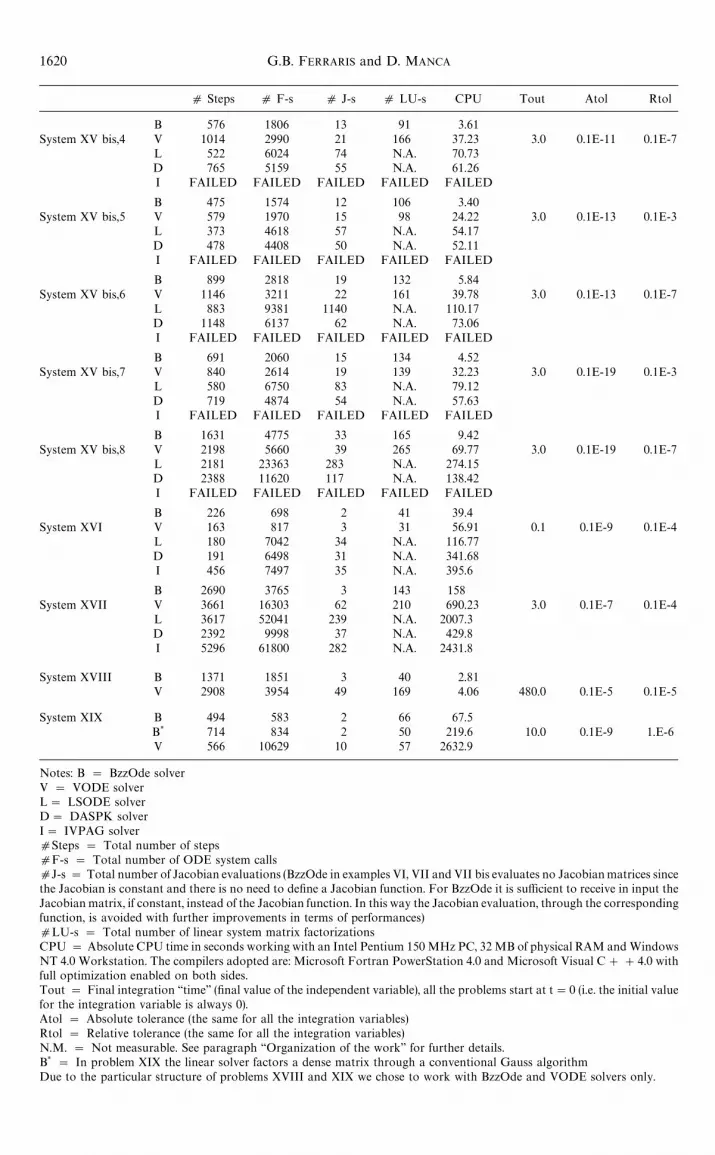
Appendix B. ODE solvers performance comparison

d Steps d F-s d J-s d LU-s CPU Tout Atol Rtol

B 270 327 18 52 N.M.System I V 250 325 5 50 N.M. 50.0 0.1E-9 0.1E-4

L 298 480 47 N.A. N.M.D 306 527 43 N.A. N.M.I 560 768 49 N.A. N.M.

B 221 311 12 53 N.M.System II V 235 334 4 40 N.M. 400.0 0.1E-9 0.1E-4

L 178 319 34 N.A. N.M.D 273 486 30 N.A. N.M.I 447 866 44 N.A N.M.

B 513 585 26 130 N.M.System II bis V 564 803 12 112 N.M. 0.4E#11 0.1E-7 0.1E-3

L 399 487 86 N.A N.M.D 484 699 83 N.A. N.M.I 4867 6381 272 N.A. N.M.

B 765 1275 40 181 N.M.System III V 925 1604 27 220 N.M. 300.0 0.1E-9 0.1E-4


B 779 1194 42 185 N.M.System III bis V 1027 1644 27 223 N.M. 300.0 0.1E-9 0.1E-4


B 425 682 20 112 N.M.System IV V 371 658 15 88 N.M. 500.0 0.1E-9 0.1E-4




B 172 262 4 28 3.97E-2System V V 164 245 3 28 3.16E-2 0.4E-1 0.1E-9 0.1E-4

L 145 502 17 N.A. 2.28E-2D 196 747 25 N.A. 5.2E-2I 360 921 26 N.A. 0.11

B 252 339 0 101 N.M.System VI V 101 147 7 40 N.M. 10.0 0.1E-9 0.1E-1

L 160 254 71 N.A. N.M.D 286 713 304 N.A. N.M.I FAILED FAILED FAILED FAILED FAILED

B 302 350 0 31 2.32E-2System VII V 5885 6423 99 309 0.4928 5.0 0.1E-2 0.1E-5

L 5569 6461 332 N.A. 0.3324D 6846 9109 8 N.A. 0.5912I 1907 2019 119 N.A. 0.1832

B 3251 5064 0 428 0.254System VII bis V FAILED FAILED FAILED FAILED FAILED 10.0 0.1E-2 0.1E-5

L FAILED FAILED FAILED FAILED FAILEDD 17104 17525 38 N.A. 1.3748I FAILED FAILED FAILED FAILED FAILED

B 201 288 21 64 N.M.System VIII V 153 217 3 41 N.M. 10.0 0.1E-9 0.1E-4


B 163 222 11 47 N.M.System IX V 111 175 4 41 N.M. 100.0 0.1E-9 0.1E-4


B 3020 5408 304 412 5.85E-2System X V FAILED FAILED FAILED FAILED FAILED 1000.0 0.1E-9 0.1E-4

L FAILED FAILED FAILED FAILED FAILEDD FAILED FAILED FAILED FAILED FAILEDI FAILED FAILED FAILED FAILED FAILED

B 3563 5876 239 964 0.236System XI V 3107 5175 80 6663 0.2432 1000.0 0.1E-8 0.1E-3

L 3075 6085 537 N.A. 0.1628D 3037 6511 468 N.A. 0.2432I 11529 15954 812 N.A. 0.903

B 924 1106 93 264 4.61E-2System XII V FAILED FAILED FAILED FAILED FAILED 1.E#10 0.1E-9 0.1E-4


B 645 733 65 198 3.11E-2System XIII V FAILED FAILED FAILED FAILED FAILED 1.E#18 0.1E-9 0.1E-4


B 906 1366 35 212 8.11E-2System XIV V FAILED FAILED FAILED FAILED FAILED 1.E#8 0.1E-9 0.1E-4




B 72 476 5 23 0.751System XV,1 V 80 651 7 24 7.72 3.0 0.1E-9 0.1E-3

L 59 1241 16 N.A. 14.55D 88 3091 41 N.A. 36.14I FAILED FAILED FAILED FAILED FAILED

B 84 501 5 27 0.901System XV,2 V 95 669 7 26 7.98 3.0 0.1E-9 0.1E-7


B 107 515 5 26 0.851System XV,3 V 99 658 7 21 7.78 3.0 0.1E-11 0.1E-3


B 152 612 5 31 1.11System XV,4 V 220 1153 9 44 12.74 3.0 0.1E-11 0.1E-7


B 139 572 5 25 0.992System XV,5 V 195 801 7 32 9.63 3.0 0.1E-13 0.1E-3


B 222 809 6 33 1.51System XV,6 V 392 1346 9 48 16.37 3.0 0.1E-13 0.1E-7


B 263 878 7 42 1.57System XV,7 V 300 1004 8 66 12.37 3.0 0.1E-19 0.1E-3


B 576 1707 12 52 3.15System XV,8 V 724 1890 13 95 23.29 3.0 0.1E-19 0.1E-7


B 258 1028 9 66 2.13System XV bis,1 V 277 1275 12 56 15.47 3.0 0.1E-9 0.1E-3


















B 226 698 2 41 39.4System XVI V 163 817 3 31 56.91 0.1 0.1E-9 0.1E-4

L 180 7042 34 N.A. 116.77D 191 6498 31 N.A. 341.68I 456 7497 35 N.A. 395.6

B 2690 3765 3 143 158System XVII V 3661 16303 62 210 690.23 3.0 0.1E-7 0.1E-4

L 3617 52041 239 N.A. 2007.3D 2392 9998 37 N.A. 429.8I 5296 61800 282 N.A. 2431.8

System XVIII B 1371 1851 3 40 2.81V 2908 3954 49 169 4.06 480.0 0.1E-5 0.1E-5

System XIX B 494 583 2 66 67.5B* 714 834 2 50 219.6 10.0 0.1E-9 1.E-6V 566 10629 10 57 2632.9

Notes: B " BzzOde solverV " VODE solverL" LSODE solverD" DASPK solverI" IVPAG solverdSteps " Total number of stepsdF-s " Total number of ODE system callsdJ-s "Total number of Jacobian evaluations (BzzOde in examples VI, VII and VII bis evaluates no Jacobian matrices sincethe Jacobian is constant and there is no need to define a Jacobian function. For BzzOde it is sufficient to receive in input theJacobian matrix, if constant, instead of the Jacobian function. In this way the Jacobian evaluation, through the correspondingfunction, is avoided with further improvements in terms of performances)dLU-s " Total number of linear system matrix factorizationsCPU "Absolute CPU time in seconds working with an Intel Pentium 150 MHz PC, 32 MB of physical RAM and WindowsNT 4.0 Workstation. The compilers adopted are: Microsoft Fortran PowerStation 4.0 and Microsoft Visual C##4.0 withfull optimization enabled on both sides.Tout " Final integration ‘‘time’’ (final value of the independent variable), all the problems start at t"0 (i.e. the initial valuefor the integration variable is always 0).Atol " Absolute tolerance (the same for all the integration variables)Rtol " Relative tolerance (the same for all the integration variables)N.M. " Not measurable. See paragraph ‘‘Organization of the work’’ for further details.B*

" In problem XIX the linear solver factors a dense matrix through a conventional Gauss algorithmDue to the particular structure of problems XVIII and XIX we chose to work with BzzOde and VODE solvers only.


Appendix C. How to obtain the BzzOde package

Non-profit organizations can request as freewaresoftware the BzzOde package to the following e-mailaddress:

[email protected]

The BzzOde package comprises:

f the BzzOde libraries for the Microsoft VisualC##4.0 or higher compiler,

f the C## tests sources of all the problems (I-XIX)presented in the paper.

The operating systems supported by the MicrosoftVisual C##4.0 or higher compiler are WindowsTM95 and WindowsTM NT 4.0.

The libraries and the source codes must not be usedfor commercial purposes. The use for scientific pur-poses must be quoted in any publication.


Documents

BzzOde: a new C++ class for the solution of stiff and non-stiff ordinary differential equation systems