The STIFF ODEBackward Euler and implicit ODE solvers

MATH1902: Numerical Solution of Differential Equationshttp://people.sc.fsu.edu/∼jburkardt/classes/math1902 2020/stiff/stiff.pdf

A zigzag path is a sign of trouble!

Stiff equations and implicit methods

So far, our ODE solvers have used an explicit formula for the next approximation. But such methodscan fail if they encounter a “stiff” differential equation, which results in an enormous errors unlessa small step size is used. We develop implicit ODE solvers that can handle such problems.

1 Vocabulary: explicit versus implicit

The word “explicit” comes from Latin, meaning unfolded or unwrapped, and “implicit” naturally has theopposite meaning. In mathematics and computation, we are used to explicit formulas, which describe somequantity of interest in terms of the values of other, known quantities. The area of a circle is an explicitfunction of its radius:

A = πr2

However, there are many situations in which we express the relationship among a set of variables in a waythat makes it difficult, or impossible, to unfold the information into an explicit formula. Consider thisexample:

x2 + xy − y2 = 19

If we are given a pair of values (x, y), we can determine whether they satisfy this relationship. The values(4,3) work. But if x = 5, what is the value of y? It is not possible to rearrange these terms to have anexplicit form, along the lines of y = formula involving only x.

Implicit equations occur in various applications, and we will see such an example in this topic, which involvesmethods of dealing with what are known as “stiff” differential equations.

1

2 stiff deriv.m defines a surprisingly difficult ODE

Consider the following differential equation, which we will nickname the “stiff ODE”:

y′ = 50(cos(t)− y)

to be solved over the interval 0 ≤ t ≤ 1 with initial condition y(0) = 0.

We can write a MATLAB function stiff deriv(t,y) which returns the value of this right hand side function,and hence defines the stiff ODE.

3 stiff solution.m evaluates the exact solution

The exact solution of this stiff ODE is;

y(t) = 50sin(t) + 50 cos(t)− 50e−50t

2501

The appearance of the exponential function in this formula is a bit of a surprise, and, it turns out, willcause us some problems very shortly. However, we can easily write a MATLAB function stiff solution(t) toevaluate this formula. (Remember that an exponential expression like −50e−50t becomes -50 * exp(-50*t)

in MATLAB.)

If we plot this function, it might at first not look difficult or dangerous, although you might notice that theslope is very steep at t = 0, and there is a sharp bend shortly afterwards.

The exact solution of the stiff ODE.

Let’s see how well we can approximate this solution.

4 stiff euler.m tries to approximate the solution

We start our exploration of this problem by using our simplest ODE solver, the Euler method. (Yes, we havebeen calling this method rk1() for a while, but now we are going to back to calling it euler()!) I am warningyou that we are going to have trouble with this problem, so it makes sense to write our solver programstiff euler.m in a way that allows us to set the number of steps n as an input quantity, so we can easily retryour solution if we are not satisfied.

2

1 function s t i f f e u l e r ( n )23 dydt = @ s t i f f d e r i v ;4 t0 = 0 . 0 ;5 t s top = 1 . 0 ;6 tspan = [ t0 , t s top ] ;7 y0 = 0 . 0 ;89 [ t1 , y1 ] = eu l e r ( dydt , tspan , y0 , n ) ;

1011 t2 = linspace ( t0 , tstop , 101 ) ;12 y2 = s t i f f s o l u t i o n ( t2 ) ;1314 plot ( t1 , y1 , ’ r−o ’ , . . .15 t2 , y2 , ’b− ’ , . . .16 ’ l i n ew id th ’ , 3 ) ;1718 return19 end

Listing 1: stiff euler.m Euler method for the stiff ODE.

Let’s try the value n = 25, which should be enough to capture the shape of the solution curve. Unfortunately,the approximation does not seem to agree well with the true solution. In particular, it does not just driftaway, it distinctly wobbles up and down. The resulting approximate zigzag curve (red) looks nothing likethe true smooth solution (blue):

Explicit Euler solution with 25 steps.

It doesn’t just seem like inaccuracy, but a wild variation in the direction. This equation is just one exampleof a stiff differential equation. Such equations include a feature that gives a typical ODE solver make astaggering, zigzag approximation to the solution. Even if we don’t know the true solution, we can usuallyrecognize that something is wrong. In general, if we reduce the stepsize dt or equivalently increase n,eventually the solution will look reasonable.

Exercise: Investigate the behavior of the Euler solution on this problem for various values of n. Comparethe solutions for n = 20, 25, 30, 35. Convince yourself that the problem will go away if our stepsize becomessmall enough.

3

5 stiff rk2.m tries a more accurate approach

We saw earlier that the Euler method can be thought of as rk1, the weakest member of the Runge-Kuttafamily of ODE solvers. It is natural to repeat our calculation using rk2, a method which is one step up inaccuracy. If we simply make a copy of our solver, but replace the word euler with rk2, we should be ableto easily create the appropriate MATLAB solver code. Here’s what I get when I repeat my calculation withn = 25:

The rk2 solution with 25 steps.

What a catastrophe! Now the approximate solution seems to be heading towards −∞. Suppose that you hadstarted out to solve this equation using the Euler method with n = 25, got a suspiciously bad answer, andtried to make things better by using n = 25 with rk2(). You would have expected that the higher accuracysolver would provide a better picture, but instead, it is in some ways much worse.

Again, I need to remind out that we can assume that if we keep increasing n, the rk2() solution will settledown and start tracking the exact solution. It’s just these strange misbehaviors are something we have notseen before in our efforts to solve ODEs.

But consider yourself very lucky that we actually know what the true solution is! In a real life situation, wewould simply have two crazy, unbelievable answers to our problem. We could suspect there was somethingterribly wrong with our program. Or we might think this is simply an impossible problem to solve. Andalthough a small enough stepsize will cure the problem, it might be the case that we can’t afford to use thenecessary small steps because it will take too long for us to solve our problem.

Exercise: Investigate the behavior of the rk2() solution on this problem for various values of n. Comparethe solutions for n = 20, 25, 30, 35. Convince yourself that the problem will go away if our stepsize becomessmall enough.

6 Implicit ODE methods reference data we don’t know yet

The ODE solvers we have looked at so far have all been of the explicit or forward type. That is, when wewrite the formula for the next solution estimate y(i+1) or “ynew”, we put all the ODE derivative informationon the right hand side, evaluated at the previous time t(i) or “told” and previous solution y(i) or “yold”.And that’s why the Euler method can be thought of as drawing the tangent line at the current solution, and

4

following it forward in time a small distance. We write an expression that approximates the derivative

dydt(told,yold) ≈ ynew - yold

tnew - told=

ynew - yold

dt

and then solve for ynew:

1 ynew = yold + dt ∗ dydt ( to ld , yold ) ;

A different approach to solving ODE’s is known as the family of implicit or backward methods. To makean implicit version of the Euler method, we start out by writing the Euler update equation again, except thatwe evaluate the right hand side of the ODE at the “future” time tnew. In general, this would be somethinglike:

1 ynew = yold + dt ∗ dydt ( tnew , ynew ) ;

where we do have the value of tnew, but we do not know the value of ynew. It can be difficult to visualizewhat is happening, because essentially we are trying to approximate the tangent line by using a value thatis “in the future”.

It’s easy to express the backward Euler step algebraically, but now we have to figure out some way to actuallysolve it. For our first example, we will see that sometimes, if the right hand side is actually linear in theunknown function y, there is a trick to work out the solution.

7 Applying the backward Euler method to our stiff ODE

Let us try using the backward Euler approach for our stiff example. Instead of the forward Euler approxi-mation:

1 y ( i +1) = y( i ) + dt ∗ 50 .0 ∗ cos ( t ( i ) ) − dt ∗ 50 ∗ y ( i ) % eva lua t e at ( to ld , yo ld )

Listing 2: Explicit Euler update step.

we now have to pose the following backward Euler approximation, and solve it for y(i+1):

1 y ( i +1) = y( i ) + dt ∗ 50 .0 ∗ cos ( t ( i +1) ) − dt ∗ 50 ∗ y ( i +1) % eva lua t e at ( tnew , ynew)

Listing 3: Implicit Euler update step.

This is an implicit formula for y(i+1). However, for this particular ODE, it turns out that we can “unfold”the formula into an explicit version by doing the appropriate algebra. This only happens for special cases,and we will later have to deal with what to do when the implicit equation can’t be solved.

To crack this particular nut, we will try to rearrange the formula so that it tells us how to evaluate y(i+1).For this case, it’s not too hard to work out what the implicit Euler update should be:

y(i+1) = y(i) + dt * 50.0 * cos ( t(i+1) ) - dt * 50 * y(i+1)

y(i+1) + dt * 50 * y(i+1) = y(i) + dt * 50.0 * cos ( t(i+1) )

( 1.0 + dt * 50 ) * y(i+1) = y(i) + dt * 50.0 * cos ( t(i+1) )

y(i+1) = ( y(i) + dt * 50.0 * cos ( t(i+1) ) ) / ( 1.0 + 50.0 * dt )

And look at that! Now we have an explicit formula for y(i+1) that we can use in our solution strategy.

1 function s t i f f b a c kw a r d e u l e r e x p l i c i t ( n )23 t0 = 0 . 0 ;4 t s top = 1 . 0 ;5 tspan = [ t0 , t s top ] ;

5

6 y0 = 0 . 0 ;78 dt = ( t s top − t0 ) / n ;9 t1 (1 ) = t0 ;

10 y1 (1 ) = y0 ;1112 for i = 1 : n13 t1 ( i +1) = t1 ( i ) + dt ;14 y1 ( i +1) = ( y1 ( i ) + dt ∗ 50 .0 ∗ cos ( t1 ( i +1) ) ) / ( 1 .0 + 50 .0 ∗ dt ) ;15 end1617 return18 end

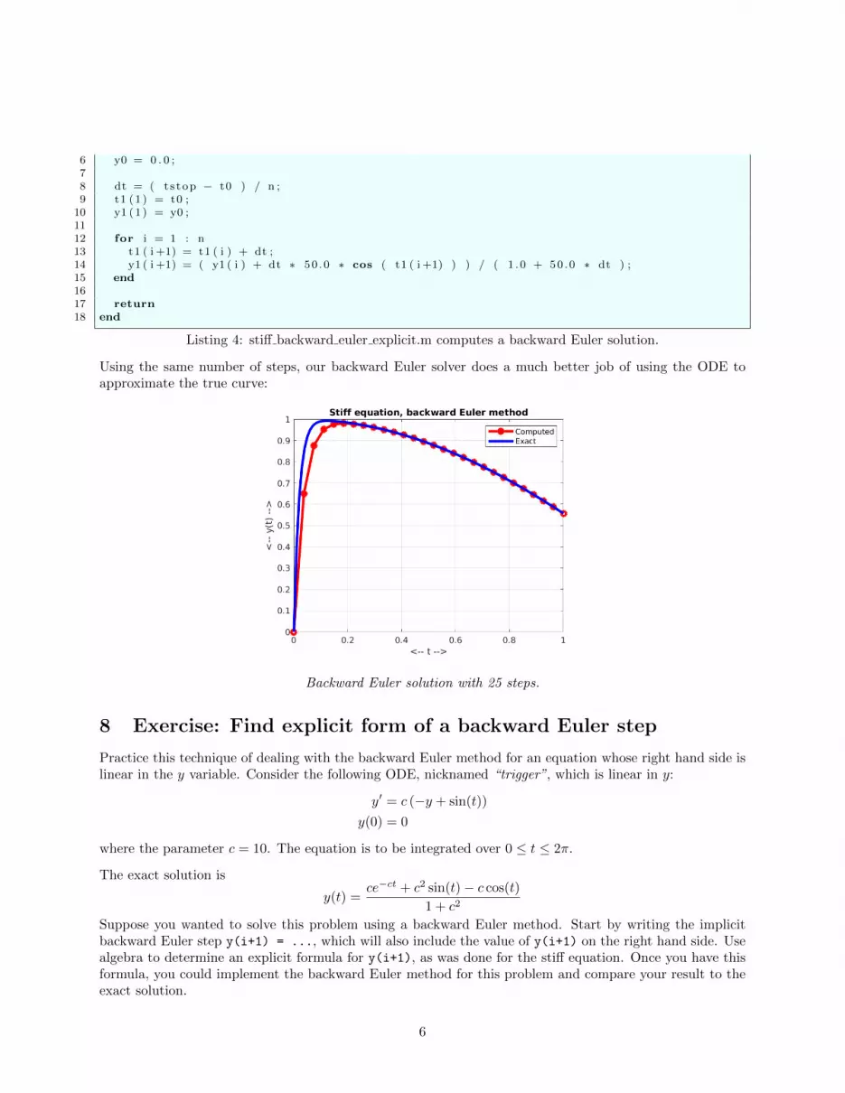
Listing 4: stiff backward euler explicit.m computes a backward Euler solution.

Using the same number of steps, our backward Euler solver does a much better job of using the ODE toapproximate the true curve:

Backward Euler solution with 25 steps.

8 Exercise: Find explicit form of a backward Euler step

Practice this technique of dealing with the backward Euler method for an equation whose right hand side islinear in the y variable. Consider the following ODE, nicknamed “trigger”, which is linear in y:

y′ = c (−y + sin(t))

y(0) = 0

where the parameter c = 10. The equation is to be integrated over 0 ≤ t ≤ 2π.

The exact solution is

y(t) =ce−ct + c2 sin(t)− c cos(t)

1 + c2

Suppose you wanted to solve this problem using a backward Euler method. Start by writing the implicitbackward Euler step y(i+1) = ..., which will also include the value of y(i+1) on the right hand side. Usealgebra to determine an explicit formula for y(i+1), as was done for the stiff equation. Once you have thisformula, you could implement the backward Euler method for this problem and compare your result to theexact solution.

6

9 Solving an implicit equation

Turning the implicit backward Euler step into an explicit formula work for the special case where the righthand side is linear in the unknown y. Of course, we can expect that most ODE’s will not have this specialstructure, which means we are stuck unless we can solve the implicit algebraic equation involving y(i+1). Inorder to use the backward Euler method for a wider range of problems, we need to know how to approximatelysolve an implicit equation.

Luckily, computational methods are available that can usually provide a good estimated solution to implicitequations. The key to this approach is to use an implicit equation solver such as MATLAB’s fsolve() function,which is part of the Optimization Toolbox. A similar function, with the same name, is also a built-in partof the Octave program.

In its simplest form, fsolve() can try to solve an implicit equation by a command like

1 x = f s o l v e ( @func , x0 ) ;

Listing 5: Solving an implicit equation using fsolve().

Here:

• x0 is an initial guess for the solution,• func() is the name of a MATLAB code which defines the implicit equation,• x is the approximate solution.

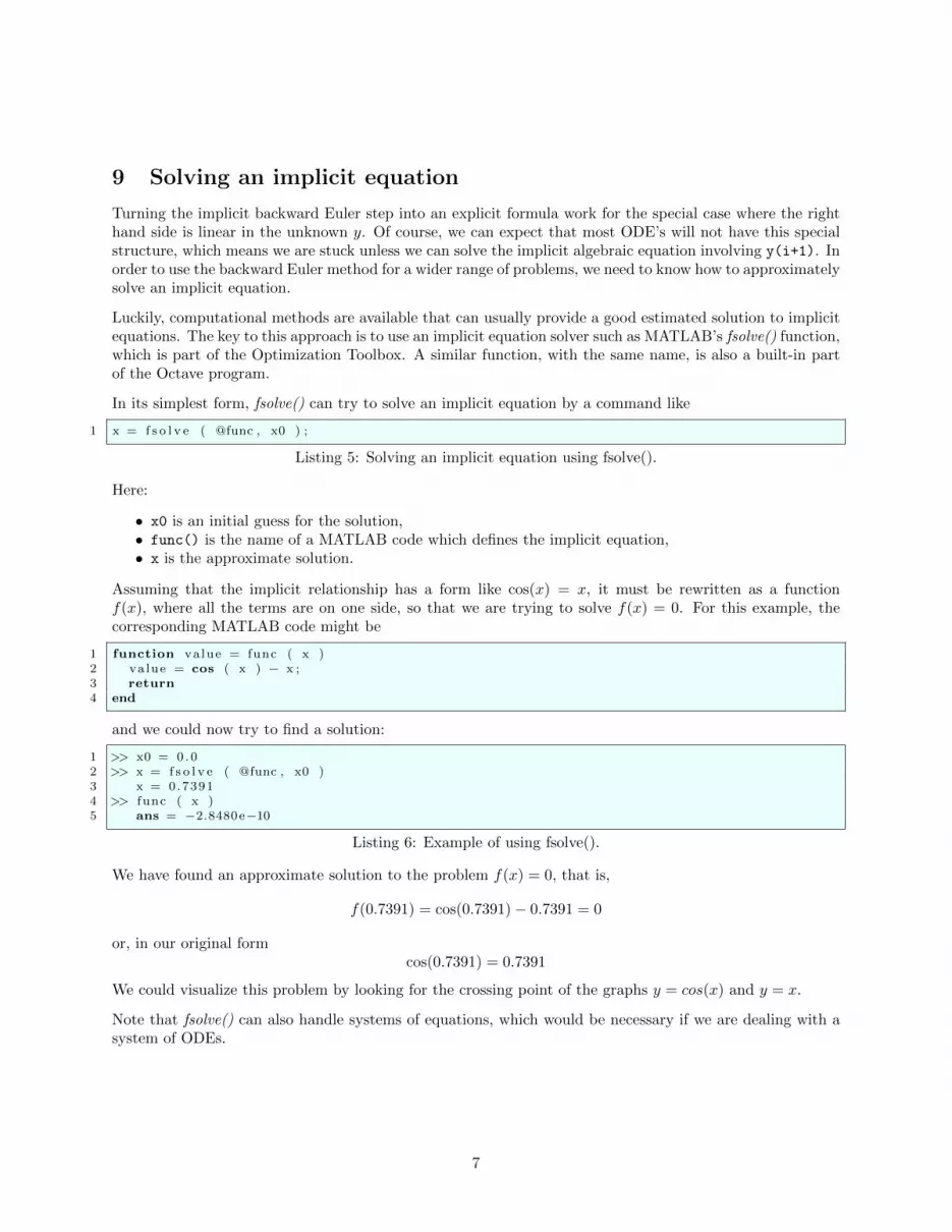
Assuming that the implicit relationship has a form like cos(x) = x, it must be rewritten as a functionf(x), where all the terms are on one side, so that we are trying to solve f(x) = 0. For this example, thecorresponding MATLAB code might be

1 function value = func ( x )2 value = cos ( x ) − x ;3 return4 end

and we could now try to find a solution:

1 >> x0 = 0 .02 >> x = f s o l v e ( @func , x0 )3 x = 0.73914 >> func ( x )5 ans = −2.8480e−10

Listing 6: Example of using fsolve().

We have found an approximate solution to the problem f(x) = 0, that is,

f(0.7391) = cos(0.7391)− 0.7391 = 0

or, in our original formcos(0.7391) = 0.7391

We could visualize this problem by looking for the crossing point of the graphs y = cos(x) and y = x.

Note that fsolve() can also handle systems of equations, which would be necessary if we are dealing with asystem of ODEs.

7

10 A backward Euler solver using fsolve()

When we used the forward Euler method, we were able to put the ODE solver into a separate function thatwould work with any ODE. Now, with our stiff example, we started with the right hand side, and had to dothe algebra on our own, and then set up a code that only works for that problem. We really want to be ableto write a general backward Euler solver, with the signature

1 function [ t , y ] = backward euler ( dydt , tspan , y0 , n )

Listing 7: Signature for backward Euler code.

which we can use just like the euler() code, so that we only have to write a function that defines the righthand side. We can create such a general backward Euler ODE solver thanks to the existence of the MATLABfsolve() function.

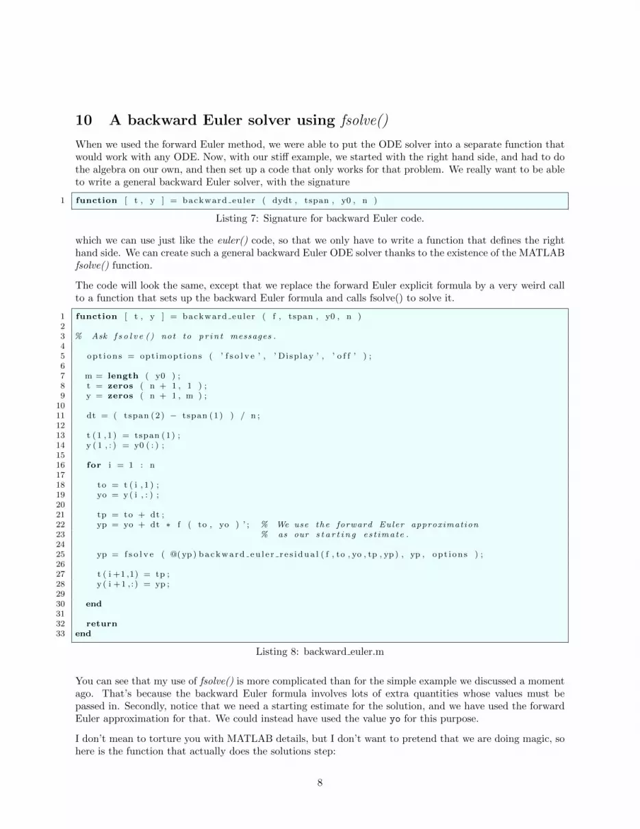
The code will look the same, except that we replace the forward Euler explicit formula by a very weird callto a function that sets up the backward Euler formula and calls fsolve() to solve it.

1 function [ t , y ] = backward euler ( f , tspan , y0 , n )23 % Ask f s o l v e () not to p r in t messages .45 opt ions = opt imopt ions ( ’ f s o l v e ’ , ’ Display ’ , ’ o f f ’ ) ;67 m = length ( y0 ) ;8 t = zeros ( n + 1 , 1 ) ;9 y = zeros ( n + 1 , m ) ;

1011 dt = ( tspan (2 ) − tspan (1) ) / n ;1213 t (1 , 1 ) = tspan (1) ;14 y ( 1 , : ) = y0 ( : ) ;1516 for i = 1 : n1718 to = t ( i , 1 ) ;19 yo = y( i , : ) ;2021 tp = to + dt ;22 yp = yo + dt ∗ f ( to , yo ) ’ ; % We use the forward Euler approximation23 % as our s t a r t i n g es t imate .2425 yp = f s o l v e ( @(yp ) backward eu l e r r e s i dua l ( f , to , yo , tp , yp ) , yp , opt ions ) ;2627 t ( i +1 ,1) = tp ;28 y ( i +1 , : ) = yp ;2930 end3132 return33 end

Listing 8: backward euler.m

You can see that my use of fsolve() is more complicated than for the simple example we discussed a momentago. That’s because the backward Euler formula involves lots of extra quantities whose values must bepassed in. Secondly, notice that we need a starting estimate for the solution, and we have used the forwardEuler approximation for that. We could instead have used the value yo for this purpose.

I don’t mean to torture you with MATLAB details, but I don’t want to pretend that we are doing magic, sohere is the function that actually does the solutions step:

8

1 function value = backward eu l e r r e s i dua l ( f , to , yo , tp , yp )2 value = yp − yo − ( tp − to ) ∗ ( f ( tp , yp ) ) ’ ;3 return4 end

Listing 9: Code to evaluate the backward Euler relation.

11 stiff backward euler() repeats our computation

Even though we’ve already solved our stiff ODE with an explicit formula, it’s a good idea to test out ournew code and see if its solution matches our previous result.

The important thing to note is that, by using fsolve() to handle the implicit equation, we now have abackward Euler ODE solver that can be used in the exact same way as our familiar codes like euler() andrk2():

1 function s t i f f b a c kwa r d e u l e r ( n )23 dydt = @ s t i f f d e r i v ;4 t0 = 0 . 0 ;5 t s top = 1 . 0 ;6 tspan = [ t0 , t s top ] ;7 y0 = 0 . 0 ;8 %9 % Same format as i f we were c a l l i n g the Euler code . . .

10 %11 [ t1 , y1 ] = backward euler ( dydt , tspan , y0 , n ) ;1213 return14 end

The moral is, if you have a stiff equation for which you need to use the backward Euler method, then youcan go ahead and try to rewrite the method as an explicit formula, which will avoid the cost of an implicitfunction solution procedure. But if you can’t rewrite it, or don’t want to, you can use a version like thiswhich will deal with the implicit function automatically.

12 The QUADEX ODE

The “quadex” ODE has a solution that looks like a quadratic (a parabola). However, getting this parabolicsolution is difficult because the equation is stiff. Small computational errors can blow up exponentially.

The ODE is

y′ = 5 ∗ (y − t2)

y(0) =2

25

to be solved over the interval 0 ≤ t ≤ 2.

The exact solution isy(t) = ce5t + t2 + 2t/5 + 2/25

where, for our initial condition, c = 0. Thus, our solution is actually a parabola, but for any other initialcondition, the exponential term would be active. These nearby exponential solutions will give us trouble.

9

Try to solve this problem twice, getting an approximately parabolic answer each time. The first time, usethe Euler method, and the second time use the backward Euler method. For each solution attempt, try thevalues of n = 25, 250, and then n = 2500.

13 Homework #7

Send the final plots (n = 2500) for your two solutions to the quadex problem via email to trenchea@pitt.edu

14 Extra credit

Try to solve the “hockeystick” ODE, which has the form:

y′ =−yc+ y

y(1) = 1

where the parameter c = 0.0001. The equation is to be solved over the interval 0 ≤ t ≤ 4.

I don’t have a formula for the exact solution. But what I do know is that the exact solution is alwayspositive. If you don’t use enough steps when trying to solve this problem, you will get a plot that looks likea straight line. But the problem is called the “hockeystick” for a reason!

10