arX

iv:p

hysi

cs/0

5070

30v3

[ph

ysic

s.cl

ass-

ph]

20

Sep

2005

Stiff dynamics of electromagnetic two-body motion

Jayme De Luca∗

Universidade Federal de Sao Carlos,

Departamento de Fısica

Rodovia Washington Luis, km 235

Caixa Postal 676, Sao Carlos,

Sao Paulo 13565-905

(Dated: February 2, 2008)

Abstract

We study the stability of circular orbits of the electromagnetic two-body problem in an electro-

magnetic setting that includes retarded and advanced interactions. We give a method to derive

the equations of tangent dynamics about circular orbits up to nonlinear terms and we derive the

linearized equations explicitly. In particular we study the normal modes of the linearized dynamics

that have an arbitrarily large imaginary eigenvalue. These large imaginary eigenvalues define fast

frequencies that introduce a fast (stiff ) timescale into the dynamics. As an application of Dirac’s

electrodynamics of point charges with retarded-only interactions, we study the conditions for the

two charges to perform a fast gyrating motion of small radius about a circular orbit. The fast

gyration defines an angular momentum of the order of the orbital angular momentum, a vector

that rotates in the orbital plane at a frequency of the order of the orbital frequency and causes

a gyroscopic torque. We explore a consequence of this multiscale solution, i.e; the resonance

condition that the angular momentum of the stiff spinning should rotate exactly at the orbital

frequency. The resonant orbits turn out to have angular momenta that are integer multiples of

Planck’s constant to a good approximation. Among the many qualitative agreements with quan-

tum electrodynamics (QED), the orbital frequency of the resonant orbits are given by a difference

of two eigenvalues of a linear operator and the emission lines of QED agree with our predictions

within a few percent.

∗author’s email address:deluca@df.ufscar.br

1

I. INTRODUCTION

We study the Lyapunov stability of quasi-circular orbits of the electromagnetic two-body

problem, a dynamical system with implicitly-defined delay. The motivation is to understand

the balancing of the fast dynamics described by the delay equations for particle separations

in the atomic magnitude. We give an economical method to derive the linearized equations

of motion about circular orbits. We work in a generalized electromagnetic setting where the

field of the point charge is a linear combination of the advanced and the retarded Lienard-

Wiechert fields with an arbitrary coefficient [1], henceforth called the Eliezer setting (ES)

(see Appendix A). We study in detail a specific feature of the tangent dynamics; The stiff

normal modes of the linearized dynamics, that have an arbitrarily large imaginary eigen-

value and introduce a fast timescale in the dynamics. The derivation of the fast normal

modes of tangent dynamics is our main technical contribution to the understanding of this

dynamical system. For some special cases of the ES we find a remarkable quasi-degeneracy

of the tangent dynamics; these cases are Dirac’s theory with retarded-only fields, the action-

at-a-distance electrodynamics and the dissipative Fokker theory of Ref. [2] (see Appendix

B). Last, we discuss the dynamics of the hydrogen atom in Dirac’s electrodynamics with

retarded-only fields, the special case of the ES of greatest relevance to physics. Having

recognized the existence of the fast dynamics near circular orbits, our method to find the

trajectory starts by balancing the fast dynamics near a tentative circular orbit. We inves-

tigate the conditions for the dynamics to execute a fast gyrating motion about a circular

orbit, henceforth called spinning and illustrated in Fig. 1. This fast gyration defines an an-

gular momentum vector of the order of the orbital angular momentum of the unperturbed

circular orbit. This angular momentum of spinning is a vector that rotates in space with

a frequency of the order of the orbital frequency. We experiment with a typical necessary

condition for such multiscale solution; the resonance condition that the angular momentum

of spinning rotates exactly at the orbital frequency. This resonance condition turns out to

be satisfied precisely in the atomic magnitude. We predict several features of the hydrogen

atom of quantum electrodynamics (QED) [3] with good precision and qualitative detail. The

frequencies of the resonant orbits agree with the lines of QED within a few percent average

deviation. There is also a large body of qualitative agreement with QED; (i) the emitted

frequency is given by a difference of two linear eigenvalues (the Rydberg-Ritz principle) (ii)

2

the resonant orbits have angular momenta that are approximate multiples of a basic angu-

lar momentum. This basic angular momentum agrees well with Planck’s constant and (iii)

the angular momentum of the fast spinning dynamics is of the order of the orbital angular

momentum.

Dirac’s 1938 work [1] on the electrodynamics of point charges gave complex delay equa-

tions that were seldom studied. Eliezer generalized Dirac’s method of covariant subtraction

of infinities in 1947[4] to include advanced interactions naturally in the electrodynamics of

point charges (the ES) [4]. Among the few dynamics of point charges investigated, another

early result of Eliezer [5–8] revealed a surprising result (henceforth called Eliezer’s theorem);

An electron moving in the Coulomb field of an infinitely massive proton can never fall into

the proton by radiating energy. The result was generalized to motions in arbitrary attractive

potentials [6], as well as to tridimensional motions with self-interaction in a Coulomb field

[7, 8], finding that only scattering states are possible. Since our model has the dynamics

of Eliezer’s theorem as the infinite-mass limit, a finite mass for the proton is essential for a

physically meaningful dynamics; If the proton has a finite mass, there is no inertial frame

where it rests at all times, and this in turn causes delay because of the finite speed of light.

A finite mass for the proton is what brings delay into the electromagnetic two-body dynam-

ics, with its associated fast dynamics. This infinite-mass limit is a singular limit, because

the equations of motion pass from delay equations to ordinary differential equations! Our

understanding of this two-body dynamics might prove useful for atomic physics and perhaps

we can understand QED as the effective theory of this complex stiff dynamics with delay.

We shall describe the two-body motion in terms of the familiar center-of-mass coordinates

and coordinates of relative separation, defined as the familiar coordinate-transformation that

maps the two-body Kepler problem onto the one-body problem with a reduced mass plus a

free-moving center of mass. We stress that in the present relativistic motion the Cartesian

center-of-mass vector is not ignorable, and it represents three extra coupled degrees-of-

freedom. We introduce the concept of resonant dissipation to exploit this coupling and

the many solutions that a delay equation can have. Resonant dissipation is the condition

that both particles decelerate together, i.e., the center-of-mass vector decelerates, while the

coordinates of relative separation perform an almost-circular orbit, despite of the energy

losses of the metastable center-of-mass dynamics. Last, we stress that our point charges

are not spinning about themselves, but rather gyrating about a center that is moving with

3

the circular orbit, as illustrated in Fig. 1, even though we refer to this gyrating motion as

spinning.

The road map for this paper is as follows; In Section IV we give the main technical part of

the paper; We outline our economical method to derive the tangent dynamics of the circular

orbit by expanding the implicit light-cone condition and the action to quadratic order. This

economical method shall be useful in the further research needed to derive the higher orders

and the complete unfolding of this dynamics. In this Section we also take the stiff limit

of the linear modes of tangent dynamics and introduce the fast timescale. In Section V

we give an application to atomic physics, by discussing a consequence of balancing the fast

dynamics first; This balancing defines an angular momentum of fast gyration comparable

to the orbital angular momentum, a vector that rotates in space with a slow frequency of

the order of the orbital frequency. In this section we discuss the heuristic condition that

the angular momentum of the fast spinning motion should rotate at the orbital frequency, a

resonance condition that predicts the correct atomic scales. The earlier sections are a prelude

to Section IV. In Appendix A we give the equations of motion of the electrodynamics of point

charges in the ES. Section II is a review of the circular orbit solution, to be used in Sections

IV and V. In Section III we give an action formalism for the Lienard-Wiechert sector of the

ES as a prelude to the quadratic expansions needed for the linear stability analysis of Section

IV. In Appendix B we derive the general tangent dynamics for oscillations perpendicular to

the orbital plane. The Lemma of resonant dissipation of Appendix C proves that for the

linearized equations of motion the state of resonant dissipation is impossible. In Appendix

D we discuss how the nonlinear stiff terms balance the leading dissipative term of the self-

interaction force and we estimate the radius of the stiff torus. Last, in Section VI we put

the conclusions and discussion.

II. THE CIRCULAR ORBIT SOLUTION

The circular-orbit solution of the isolated electromagnetic two-body problem of the action-

at-a-distance electrodynamics (the ES with k = −1/2, see Appendix A) is used here as the

unperturbed orbit[9, 10]. For the ES with k = −1/2, the tangent dynamics of the next

section is straightforward Lyapunov stability analysis. In the general case, ( k 6= −1/2), the

4

ES also prescribes a small force opposite to the velocity of each particle along the circular

orbit, such that the circular orbit is not an exact solution of the equations of motion. The

tangent dynamics is then the starting point of a perturbation scheme to obtain a stiff torus

near a circular orbit (the state of resonant dissipation discussed in Appendix C).

We shall use the index i = 1 for the electron and i = 2 for the proton, with masses m1 and

m2 respectively. We henceforth use units where the speed of light is c = 1 and e1 = −e2 ≡ −1

(the electronic charge). The circular orbit is illustrated in Fig. 2; the two particles move in

concentric circles with the same constant angular speed and along a diameter. The details

of this relativistic orbit will be given now; The constant angular velocity is indicated by

Ω , the distance between the particles in light-cone is rb and θ ≡ Ωrb is the angle that one

particle turns while the light emanating from the other particle reaches it (the light-cone

time lag). The angle θ is the natural independent parameter of this relativistic problem. For

orbits of the atomic magnitude the orbital frequency is given to leading order by Kepler’s

law

Ω = µθ3 + ... (1)

while the light-cone distance rb is given by

rb =1

µθ2 + ... (2)

Each particle travels a circular orbit with radius and scalar velocity defined by

r1 ≡ b1rb, (3)

r2 ≡ b2rb,

and

v1 = Ωr1 = θb1, (4)

v2 = Ωr2 = θb2,

for the electron and for the proton, respectively. The condition that the other particle turns

an angle θ during the light-cone time lag [9] is

b21 + b2

2 + 2b1b2 cos(θ) = 1, (5)

and is henceforth called the unperturbed light-cone condition. As shown in Appendix B

of Ref. [2], b1 and b2 are approximated by the Keplerian values b1 = m2/(m1 + m2) and

5

b2 = m1/(m1 + m2) plus a correction of order θ2. As discussed in Ref. [9], there is a

conserved angular momentum perpendicular to the orbital plane of the circular orbit given

by

lz =1 + v1v2 cos(θ)

θ + v1v2 sin(θ), (6)

where the units of lz are e2/c, just that we are using a unit system where e2 = c = 1. For

small values of θ the angular momentum of Eq. (6) is of the order of lz ∼ θ−1. For orbits of

the atomic magnitude, lz ≃ θ−1 is about one over the fine-structure constant, α−1 = 137.036.

III. AN ACTION FOR THE LORENTZ FORCE

We introduce an action to be used as an economical means to derive the Lorentz-force

sector of the ES equations of motion with the linear combination of retarded and advanced

Lienard-Wiechert potentials. In the following we derive the tangent dynamics by expanding

this action to quadratic order. We henceforth use the dot to indicate the scalar product of

two Cartesian vectors. The Lienard-Wiechert action for the Lorentz-force sector of the ES

is

Θ = −k

∫

(1 − v1 · v2a)

r12a(1 + n12a · v2a)dt1 + (1 + k)

∫

(1 − v1 · v2b)

r12b(1 − n12b · v2b)dt1, (7)

In Eq. (7) v1 stands for the Cartesian velocity of particle 1 at time t1 and v2a and v2b

stand for the Cartesian velocities of particle 2 at the advanced and at the retarded time t2

respectively. The vector n12a is a unit vector connecting the advanced position of particle 2

at time t2 to the position of particle 1 at time t1, vector n12b is a unit vector connecting the

retarded position of particle 2 at time t2 to the position of particle 1 at time t1 and (Below

Eq. (8) of Ref. [2] this normal is defined to the opposite direction, but it was used correctly

in Eq. (19) of Ref. [2] ). Notice that each integral on the right-hand-side of Eq. (7) can be

cast in the familiar form

∫

(1 − v1 · v2c)

r12(1 + n12·v2c

c)dt1 ≡ −

∫

(V − v1 · A)dt, (8)

where V and A are the Lienard-Wiechert scalar potential and the Lienard-Wiechert vector

potential respectively. We have introduced the quantity c = ±1 in the denominator of Eq.

(8) such that c = 1 represents the advanced interaction while c = −1 represents the retarded

6

interaction. The quantities of particle 2 in Eq. (8) are to be evaluated at the time t2 defined

implicitly by

t2 = t1 +r12

c, (9)

where c = ±1 describes the advanced and the retarded light cones, respectively. Because of

this decomposition into V and A parts, we henceforth call Eq. (8) the VA interaction. The

minimization of action (7) plus the kinetic energy of particle 1 yields the equations of motion

for particle 1 suffering the Lorentz-force of the Lienard-Wiechert potentials produced by the

other particle (see Eq. (58) ), as shown for example in Ref.[11]).

Besides the Lorentz-force, which is the Lagrangian part of the ES equations of motion,

there is also the dissipative self-interaction force in Eq. (58). The shortest way to write the

ES equations of tangent dynamics is to add this term to the Lagrangian equations of motion,

watching carefully for the correct multiplicative factor. The stiff limit is determined by the

largest-order derivative appearing in the linearized equations of motion of Appendix A. In

this approximation, the contribution of the self-interaction force of the ES to the linearized

dynamics about a circular orbit is simply given by the Abraham-Lorentz -Dirac force

Frad =2

3(1 + 2k)a, (10)

with a renormalized charge. The contribution of the other smaller nonlinear terms will be

given elsewhere (one such nonlinear term is used in the estimate of Appendix D).

IV. EXPANDING THE ACTION TO FIRST ORDER: MINIMIZATION

In the following sections we substitute the circular orbit of Eqs. (3) and (4) plus a planar

perturbation into Eliezer’s action (7). We then expand the action up to the quadratic order

to yield the linearized equations of motion. Our economical derivation of the stability

equations anticipates the need to study the stability of the stiff torus near the circular orbit,

a novel solution of the two-body problem as illustrated in Fig 2. In this work we keep to the

linear stability of circular orbits, which is done with the quadratic expansion of the action.

The variational equations for planar perturbations are decoupled from the equation for

transverse perturbations. We perform the planar stability analysis using complex gyroscopic

coordinates rotating at the frequency Ω of the unperturbed circular orbit; The coordinates

7

(xj , yj) of each particle are defined by two complex numbers ηj and ξj ( j = 1 for electron

and j = 2 for proton) according to

uj ≡ xj + iyj ≡ rb exp(iΩt)[dj + 2ηj], (11)

u∗

j ≡ xj − iyj ≡ rb exp(−iΩt)[d∗

j + 2ξj ],

where d1 ≡ b1 and d2 ≡ −b2 are defined in Eqs. (3). Because xj and yj are real, we must

have ηj ≡ ξ∗j but to obtain the variational equations it suffices to treat ηj and ξj as two

independent variables in the Lagrangian. We henceforth call the coordinates of Eq. (11) the

gyroscopic η and ξ coordinates. The d’s are real numbers if we choose the origin of times at

t = 0, but we have kept the harmless star above them to indicate complex conjugation in

anticipation to what follows. Two quantities appear so often in the calculations that we have

named them; (i) The numerator of the action (8) along circular orbits, henceforth called C,

evaluates to

C ≡ 1 + b1b2θ2 cos(θ), (12)

for either retarded (c = −1) or advanced interactions ( c = 1), and (ii) The denominator of

action (8) along circular orbits, divided by rb , henceforth called S and defined by

S ≡ 1 + b1b2θ sin(θ), (13)

again for either retarded or advanced interactions (c = ±1). For the stiff limit of Sections

V and VI we shall ignore the O(θ2) corrections and set C = S = 1. Here we shall derive

the electron’s equation of motion only (j = 1 in Eq. (11)). The equation for the proton

is completely symmetric and can be obtained by interchanging the indices. One can derive

from Eq. (11) that the electron’s velocity at time t1 is

u1 ≡ v1x + iv1y ≡ θ exp(iΩt1)[id1 + 2i(η1 − iη1], (14)

u∗

1 ≡ v1x − iv1y ≡ θ exp(−iΩt1)[−id∗

1 − 2i(ξ1 + iξ1)].

The velocity of the proton at its time t2 can be obtained by simple interchange of the indices

1 and 2, remembering that d1 = b1 is defined positive while d2 = −b2 is defined negative,

because at the same time the particles are in diametrically opposed positions on the exact

circular orbit, such that the exchange operation on the d′s is d1 ⇐⇒ −d2 (see Fig. 2).

8

The coordinates of particle 2 entering in the VA interaction of Eq. (8) are evaluated at

a time t2 in light-cone with the the present of particle 1. Because the implicit light-cone

condition has to be expanded and solved by iteration, it is convenient to define a function

ϕc as

t2 ≡ t1 +rb

c+

ϕc

Ω. (15)

The above definition is good for both the advanced and the retarded cases, c = 1 defining

the advanced light-cone and c = −1 defining the retarded light-cone and the underscore c

is to indicate that ϕc is a function of c. If the perturbation is zero then ϕc = 0 and we are

along the original circular orbit, where the light-cone lag is the constant rb. We henceforth

call t the present time of particle 1 (the electron) and we measure the evolution in terms of

the scaled-time parameter τ ≡ Ωt. The implicit definition of ϕc by the light-cone condition

involves the position of particle 2 at the advanced and the retarded time t2 as defined by

Eq. (11),

u2(τ + cθ + ϕc) ≡ rb exp(iΩt2)[d2 + 2η2(τ + cθ + ϕc)], (16)

u∗

2(τ + cθ + ϕc) ≡ rb exp(−iΩt2)[d∗

2 + 2ξ2(τ + cθ + ϕc)].

as well as the velocity of particle 2 at the advanced/retarded position

u2(τ + cθ + ϕc) ≡ iθ exp(iΩt2)[d2 + (η2 − iη2) + 2ϕc(η2 − η2)], (17)

u∗

2(τ + cθ + ϕc) ≡ −iθ exp(−iΩt2)[d∗

2 + (ξ2 + iξ2) + 2ϕc(ξ2 + ξ2)].

The linear stability analysis involves expanding the equation of motion to first order in ηk

and ξk , which in turn is determined by the quadratic expansion of the action (7) in ηk and

ξk. We must therefore carry all expansions up to the second order in the ηξ coordinates. For

example the position vector of particle 2 can be determined to second order by expanding

the arguments of η and ξ in a Taylor series about the value on the unperturbed circular

light-cone for one order only as

u2(τ + cθ + ϕc) ≃ rb exp(iΩt2)d2 + 2[η2(τ + cθ) + ϕcη2(τ + cθ)], (18)

u∗

2(τ + cθ + ϕc) ≃ rb exp(−iΩt2)d∗

2 + 2[ξ2(τ + cθ) + ϕcξ2(τ + cθ)].

9

We shall henceforth indicate the quantities of particle 2 evaluated exactly on the light-cone by

writing that quantity with a subindex c, as for example η2c ≡ η2(τ +cθ) and ξ2c ≡ ξ2(τ +cθ).

In the following we find that ϕc is linear in η and ξ to leading order, such that the next

term in the above expansion involves third order terms, which are not needed for the linear

stability analysis of the circular orbit. We shall always expand quantities evaluated at the

perturbed light-cone in a Taylor series about the unperturbed light-cone up to the order

needed, such that our method yields equations with a fixed delay. The perturbed light-cone

is expressed implicitly by the distance from the advanced/retarded position of particle 2 to

the present position of particle 1, described in gyroscopic coordinates by the modulus of the

complex number

uc ≡ u1(τ) − u2(τ + cθ + ϕc). (19)

where c = 1 describes the advanced position and c = −1 describes the retarded position.

Using Eq. (18) this complex number evaluates to

uc ≡ rb exp(iΩt2)D∗ + 2[exp(−icθ − iϕc)η1(τ) − η2c − ϕcη2c], (20)

u∗

c ≡ rb exp(−iΩt2)D + 2[exp(icθ + iϕc)ξ1(τ) − ξ2c − ϕcξ2c],

where we have factored the Ωt2 out and defined the complex number

D ≡ b2 + b1 exp(icθ + iϕc), (21)

that carries an implicit dependence on ϕc and will later be expanded to second order as well.

Notice that the star appears in the unusual first line because we are factoring Ωt2 out in Eq.

(20). At ϕc = 0 (the unperturbed circular orbit), the complex number D defined by Eq. (21)

has a unitary modulus. The last term on the right-hand side of Eq. (20) is a quadratic form

times exp(iΩt2) and in the action it only appears multiplied by a counter-rotating constant

term, i.e., a quadratic form times exp(−iΩt2), such that the product is independent of

t2. Therefore this quadratic term can be integrated by parts and the Gauge term can be

disregarded, as in any Lagrangian. We henceforth call this a quadratic Gauge simplification

and we shall use it in several expressions. This simplification applied to integrate the terms

in η2c and ξ2c of Eq. (20) by parts yields

u ≡ rb exp(iΩt2)D∗ + 2[(1 − iϕc) exp(−icθ)η1(τ) − (1 − ϕc)η2c], (22)

u∗ ≡ rb exp(−iΩt2)D + 2[(1 + iϕc) exp(icθ)ξ1(τ) − (1 − ϕc)ξ2c].

10

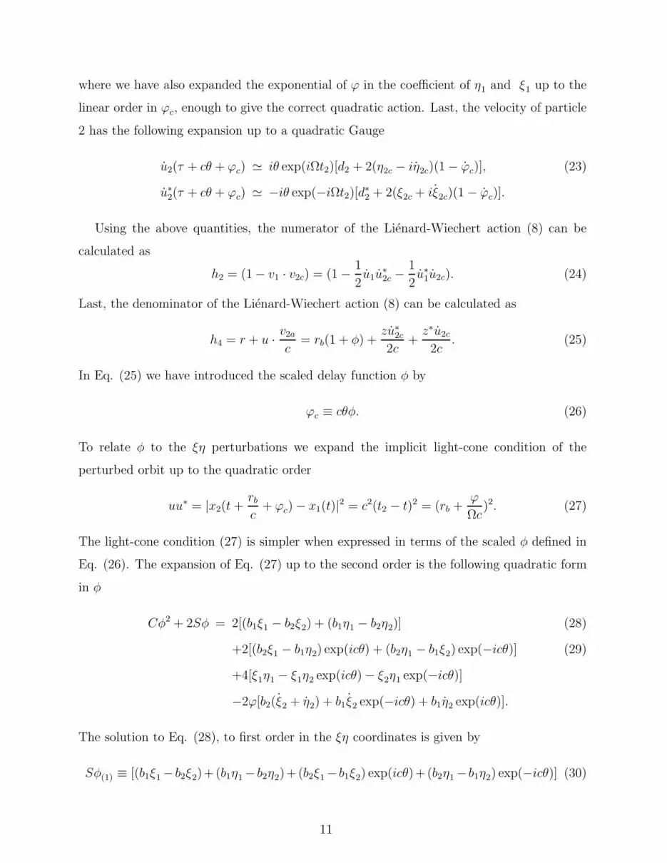
where we have also expanded the exponential of ϕ in the coefficient of η1 and ξ1 up to the

linear order in ϕc, enough to give the correct quadratic action. Last, the velocity of particle

2 has the following expansion up to a quadratic Gauge

u2(τ + cθ + ϕc) ≃ iθ exp(iΩt2)[d2 + 2(η2c − iη2c)(1 − ϕc)], (23)

u∗

2(τ + cθ + ϕc) ≃ −iθ exp(−iΩt2)[d∗

2 + 2(ξ2c + iξ2c)(1 − ϕc)].

Using the above quantities, the numerator of the Lienard-Wiechert action (8) can be

calculated as

h2 = (1 − v1 · v2c) = (1 − 1

2u1u

∗

2c −1

2u∗

1u2c). (24)

Last, the denominator of the Lienard-Wiechert action (8) can be calculated as

h4 = r + u · v2a

c= rb(1 + φ) +

zu∗

2c

2c+

z∗u2c

2c. (25)

In Eq. (25) we have introduced the scaled delay function φ by

ϕc ≡ cθφ. (26)

To relate φ to the ξη perturbations we expand the implicit light-cone condition of the

perturbed orbit up to the quadratic order

uu∗ = |x2(t +rb

c+ ϕc) − x1(t)|2 = c2(t2 − t)2 = (rb +

ϕ

Ωc)2. (27)

The light-cone condition (27) is simpler when expressed in terms of the scaled φ defined in

Eq. (26). The expansion of Eq. (27) up to the second order is the following quadratic form

in φ

Cφ2 + 2Sφ = 2[(b1ξ1 − b2ξ2) + (b1η1 − b2η2)] (28)

+2[(b2ξ1 − b1η2) exp(icθ) + (b2η1 − b1ξ2) exp(−icθ)] (29)

+4[ξ1η1 − ξ1η2 exp(icθ) − ξ2η1 exp(−icθ)]

−2ϕ[b2(ξ2 + η2) + b1ξ2 exp(−icθ) + b1η2 exp(icθ)].

The solution to Eq. (28), to first order in the ξη coordinates is given by

Sφ(1) ≡ [(b1ξ1 − b2ξ2)+(b1η1 − b2η2)+(b2ξ1 − b1ξ2) exp(icθ)+(b2η1 − b1η2) exp(−icθ)] (30)

11

As an application of the above, we derive the equations of motion for the circular orbits

of the action-at-a-distance electrodynamics [9] (the ES with k = −1/2 ). The equation of

motion for ξ1 can be calculated by expanding the VA interaction of Eq. (7) to linear order

Θ ≡ 1 − [θ2(S − 1)S + C2](b1 + b2 cos(θ)) + S(θ sin(θ) − θ2 cos(θ))b2(η1 + ξ1)

CS2, (31)

where the tilde indicates that we scaled Θ by the factor Θo = C/(rbS) (the value of Θ

along the unperturbed circular orbit). Scaling the kinetic energy with the same factor and

expanding to first order yields

T1 =−rbm1S

Cγ1

+rbθ

2m1γ1Sb1

C(η1 + ξ1), (32)

Such that the effective Lagrangian for particle 1 is

L1 ≡ T1 + Θ (33)

Since those are linear functions of ξ1, the Euler-Lagrange equation for ξ1 is simply ∂L1

∂ξ1

= 0

or

m1b1rbγ1θ2S3 = [C2 + θ2S(S − 1)](b1 + b2 cos(θ)) + S(θ sin(θ) − θ2 cos(θ))b2. (34)

This is Eq. 3.2 of Ref. [9], and the equation for η1 is the same condition by symmetry (the

reason why the circular orbit is a solution). The equation of motion for particle 2 can be

obtained by interchanging the indices 1 and 2 in Eq. (34), representing Eq. 3.3 of Ref. [9].

In the next section we carry the expansion of the action to second order, to determine the

equations of tangent dynamics.

V. EXPANDING THE ACTION TO SECOND ORDER

The next term of expansion (32) of the local kinetic energy of particle 1 can be calculated

with Eq. (14) to be

T1 = To −rbSm1

C

√

1 − |v1|2 =rbθ

2m1γ1Sb1

C(η1 + ξ1) (35)

+Srbθ

2m1γ1

2C[γ2

1(ξ1 + iξ1 + η1 − iη1)2 − (ξ1 + iξ1 − η1 + iη1)

2] + ...

12

This kinetic energy of particle 1 has the simple quadratic form defined by two coefficients

T1 =rbθ

2m1γ1Sb1

C(η1 + ξ1) (36)

+M1[η1ξ1 + i(η1ξ1 − ξ1η1) + η1ξ1] +θ2G1

2[ξ2

1 + η21 − ξ

2

1 − η21]

where M1 ≡ (1 + γ21)m1γ1rbθ

2S/Cand G1 ≡ (γ21 − 1)m1γ1θ

2S/C. We also need the solution

of Eq. (28) to second order, φ = φ(1)+ φ(2) , where φ(1) is given by Eq. (30) and φ(2) is

calculated by iteration to be

Sφ(2) = ϕ(ib2ξ1 − ib1η2 − b1η2) exp(icθ) + ϕ(ib1ξ2 − ib2η1 − b1ξ2) exp(−icθ) (37)

−ϕb2(ξ2 + η2) −1

2C[φ(1)]

2

+2[ξ1η1 − ξ1η2 exp(icθ) − ξ2η1 exp(−icθ)]

Next we expand the numerator and the denominator of action (8), Eqs. (24) and (25), up to

the quadratic order. We use the expansion of the particle separation, Eq. (20), the velocity

of particle 1 (Eq. (14)), and the expansion of the velocity of particle 2, Eq. (23). The

quadratic expansion of the action is cumbersome and must be evaluated with a symbolic

manipulation software (we have used Maple 9). Integrating by parts and disregarding Gauge

terms, we can bring this quadratic expansion to the following ” normal form for particle 1

”

Θc = − i

2B(η1ξ1 − ξ1η1) + U11ξ1η1 +

1

2N11ξ

21 +

1

2N∗

11η21 (38)

+Rcξ1ξ2c + R∗

cη1η2c + Pcξ1η2c + P ∗

c η1ξ2c +

+Yc

2(ξ1ξ2c − ξ2cξ1) +

Y ∗

c

2(η1η2c − η2cη1) +

Λc

2(ξ1η2c − η2cξ1) +

Λ∗

c

2(η1ξ1 − ξ2η1) +

+Tc

2ξ1ξ2c +

T ∗

c

2η1η2c +

Ec

2ξ1η2c +

E∗

c

2η1ξ2c

Notice that in Eq. (38) the coordinates of particle 2 appear evaluated in either the retarded

or the advanced unperturbed light-cone, which is indicated by the subindex c. The full

quadratic expansion of the action is composed of the kinetic energy plus the partial actions

of Eq. (38) evaluated at the retarded and the advanced light-cones and multiplied by the

13

respective Eliezer’s coefficient, as in Eq. (7)

L1 = T1 − kΘ+ + (1 + k)Θ− (39)

Notice in Eq. (38) the appearance of the angular-momentum-like binaries inside parenthesis,

a normalization achieved by adding a quadratic Gauge term to the Taylor series. The

coefficient of each normal-form binary is obtained by a simple Gauge-invariant combination

of derivatives, for example the magnetic field coefficient B is given by

B = i[∂2L

∂η1∂ξ1

− ∂2L

∂ξ1∂η1

]. (40)

In what follows we evaluate the expansion of the action using a symbolic software (Maple

9). The linearized Euler-Lagrange equation obtained by minimizing action (39) respect to

the function ξ1 is a linear functional involving the coordinates ξ1 , η1 , ξ2+ , η2+ , ξ2− and

η2− as well as their first and second derivatives

l1ξ(ξ1, η1, ξ2+, η2+, ξ2−, η2−) = (41)

−[(N11 + θ2G)ξ1 + θ2Gξ1] + [M1(η1 + 2iη1 − η1) − U11η1 − iBη1]

−(R∗

+ξ2+ + R∗

−ξ2−) − (Y+ξ2+ + Y−ξ2−) + (T+ξ2+ + T−ξ2−)

−(P+η2+ + P−η2−) − (Λ+η2+ + Λ−η2−) + (E+η2+ + E−η2−)

Minimization of action (39) respect to η1, ξ2 and η2 yields three more linear equations, which

together with Eq. (41) compose a system of four linear delay equations. To include the

dissipative self-interaction force into Eq. (41) we substitute θ2 = r2bΩ

2 into the definition of

M1 above Eq. (37), such that the Euler-Lagrange equation of the kinetic energy (36) respect

to ξ1 can be written as

(1 + γ21)m1γ1(S/C)r3

bΩ2(η1 + 2iη1 − η1) (42)

= r2b (S/C)

d

dt(m1γ1rbu1).

On the second line of Eq. (42) we recognize the variation of the complex momentum

m1γ1rbu1 multiplied by the factor r2b (S/C), a complexifyed version of the planar force.

To include the self-interaction into the linearized Euler-Lagrange equations, we simply add

the complexifyed planar force of Eq. (10) multiplied by the same factor r2b (S/C) into Eq.(41)

r2b (S/C)

2

3(1 + 2k)rb

d3u1

dt3≃ 2θ3

3(1 + 2k)

...u 1, (43)

14

where the dots represent derivative respect to the scaled time τ ≡ Ωt. Using definition

(11) for the gyroscopic coordinate u1 into Eq. (43) yields the offensive force of Eq. (79)

of Appendix C plus the required linearized gyroscopic version of the triple dots term. The

offensive force is a nonhomogeneous term that will be dealt with in Appendix C. In this

section we discard it and keep only the linear correction to the self force.

Addding the linear term of the self-force to the η1, ξ2 and η2 Euler-Lagrange equations

yields a system of four linear delay equations, which can be solved in general by Laplace

transform [15]. Here we shall concentrate on the separable normal mode solutions of this lin-

ear system. For that we substitute ξ1 = A exp(λτ/θ), η1 = B exp(λτ/θ), ξ2 = C exp(λτ/θ)

and η2 = D exp(λτ/θ) into the linearized equations and we assume that |λ| is an order-one

or larger quantity, which is henceforth called the stiff limit (we shall see that |λ| can take

values of about π or larger while θ is about 10−2 in the atomic magnitude). The four linear

equations in A, B, C and D have a nontrivial solution only if the determinant vanishes,

a condition that we evaluate with a symbolic manipulations software in the large-λ limit

(stiff-limit)

1 − 2(1 + 2k)θ2λ

3+

(1 + 2k)θ4λ2

9− 2

27

µ

M(1 + 2k)3θ6λ3 + ... (44)

+µθ4

M(1 +

7

λ2 +5

λ4 )[(1 + 2k) sinh(2λ) − 2(1 + 2k + 2k2) cosh2(λ)]

−2µθ4

M(1

λ+

5

λ3 )[2(1 + 2k) cosh2(λ) − (1 + 2k + 2k2) sinh(2λ)] = 0

In the special case of k = −1/2 Eq. (44) reduces to Eq. 33 of reference [2] without the

radiative terms, that are ad-hoc in the dissipative Fokker setting of Ref.[2] (this amounts

to setting k = 0 in the first line of Eq. (44) and k = −1/2 in the other two lines). In this

work we shall focus on Dirac’s retarded-only electrodynamics of point charges (Eq. (44)

with k = 0) , with the following planar-normal-mode condition in the stiff-limit

(1 +2

λxy+

7

λ2xy

+10

λ3xy

− 5

λ4xy

+ ...)(µθ4

M) exp(−2λxy) (45)

= 1 − 2

3θ2λxy +

1

9θ4λ2

xy + ...,

Comparing Eq. (45) to Eq. (78) of Appendix B we find that the quasi-degeneracy of the

stiff dynamics exists only for k = 0, (retarded-only interactions, Dirac’s theory), k = −1

(advanced-only interactions), and k = −1/2 (either the dissipative Fokker theory of Ref.[2]

or the action-at-a-distance electrodynamics).

15

VI. STIFF TORUS AS A DEFORMED CIRCULAR ORBIT

As discussed in the previous Section, in Appendix B and already explored in Ref.[2], there

is a remarkable quasi-degeneracy of the perpendicular and the planar tangent dynamics for

some special settings. Here we shall focus on Dirac’s electrodynamics with retarded-only

interactions. Both Eq. (78) and Eq. (45) with k = −1/2 in the large-λ limit reduce to

(µθ4

M) exp(−2λ) = 1, (46)

For hydrogen (µ/M) is a small factor of about (1/1824). For θ of the order of the fine

structure constant the small parameter µθ4

M∼ 10−13 multiplying the exponential function on

the left-hand side of Eq. (46) determines that Re(λ) ≡ −σ ≃ − ln(√

Mµθ4 ). For the first 13

excited states of hydrogen this σ is in the interval 14.0 < |σ| < 18.0. The imaginary part of

λ can be an arbitrarily large multiple of π, such that the general solution to Eq. (46) is

λ = −σ + πqi (47)

where i ≡√−1 and q is an arbitrary integer. Notice that the real part of λ is always

negative, such that the tangent dynamics about the circular orbit is stable in the stiff-limit.

The coefficient of the term of order 1/λ2 is the main difference between Eqs. (78) and

(45). The terms of order θ4λ2 also differ but they are much less important for θ in the

atomic range. The exact roots of Eqs. (45) and (78) near the limiting root (47) are defined,

respectively, by

λxy(θ) ≡ −σxy + πqi + iǫ1, (48)

λz(θ) ≡ −σz + πqi + iǫ2,

where ǫ1(θ) and ǫ2(θ) are real numbers of the order of θ and depending on the orbit through

θ. The stiff torus is formed from an initial circular orbit as follows; (i) The offending force

against the velocity dissipates energy and makes the electron loose radius on a slow timescale

(the radiative instability discussed in Appendix C). (ii) When the electron deviates enough

from the circular orbit, the stiff nonlinear terms compensate the offending terms (iii) Because

of this same deviation from circularity, the stiff terms also balance the real parts of Eq. (48),

the σ′s . A purely harmonic solution to the nonlinear equations of tangent dynamics appears

16

because the nonlinear stiff terms introduce a correction into Eqs. (45) and (78), as discussed

in Appendix D. The complete description of this new solution involves expanding the action

about the circular orbit to the fourth order and the coupling to the center-of-mass recoil and

shall be given elsewhere. Because of the large frequency of the stiff motion, this balancing

is established at a very small radius, as estimated by Eq. (89) of Appendix D. The motion

continues to be stiff because of the imaginary part of the λ′s of Eq. (48). We henceforth

assume that this balance is achieved near the original circular motion. As discussed in

Appendix C, the circular orbit recoils in a slow timescale to compensate the momentum

loss to the radiated energy. During the recoil the particle coordinates are described by a

composition of a translation mode and a stiff mode, both with slowly varying amplitudes,

such that the dynamics of the balanced stiff torus is described by

ξk = Ak(T ) + uk(T ) exp[(πqi + iǫρ1)Ωt/θ], (49)

Zk = ReBk(T ) + Rk(T ) exp[(πqi + iǫρ2)Ωt/θ],

where the amplitudes uk and Rk must be near the size where the nonlinearity balances the

negative real part of the linear modes. Assuming |u1| ≃ |R1| ≃ ρ, with ρ given by Eq. (89),

the angular momentum of the stiff torus along the orbital plane calculated using (49) and

disregarding fast oscillating small terms is

lx + ily = µr2bρ

2πqΩ

θb1 exp[i(ǫρ

2 − ǫρ1 + θ)Ωt/θ] (50)

=πq

θ2 ρ2 exp[i(ǫρ2 − ǫρ

1 + θ)Ωt/θ],

where on the second line of Eq. (50) we have used formula (1) for Ω and formula (2) for rb.

Notice that we chose the same q on the two perpendicular oscillations in Eq. (49), such that

the fast oscillations beat in the slow timescale. A typical nonlinear term of this dynamics is

the angular momentum of spin defined by Eq. (49). As illustrated in Fig. 1, the balancing

of the fast dynamics, Eq. (49), defines an angular-momentum vector (50) associated with

the fast spinning. This angular momentum vector rotates at a (slow! ) frequency that is

generically of the order of the orbital frequency and is determined solely by the balancing

of the fast dynamics. This slowly rotating gyroscope attached to the electron is the main

qualitative feature left after we balance the stiff delay dynamics. According to Eq. (50) this

slow frequency is

≡ Ω[1 +(ǫρ

2 − ǫρ1)

θ], (51)

17

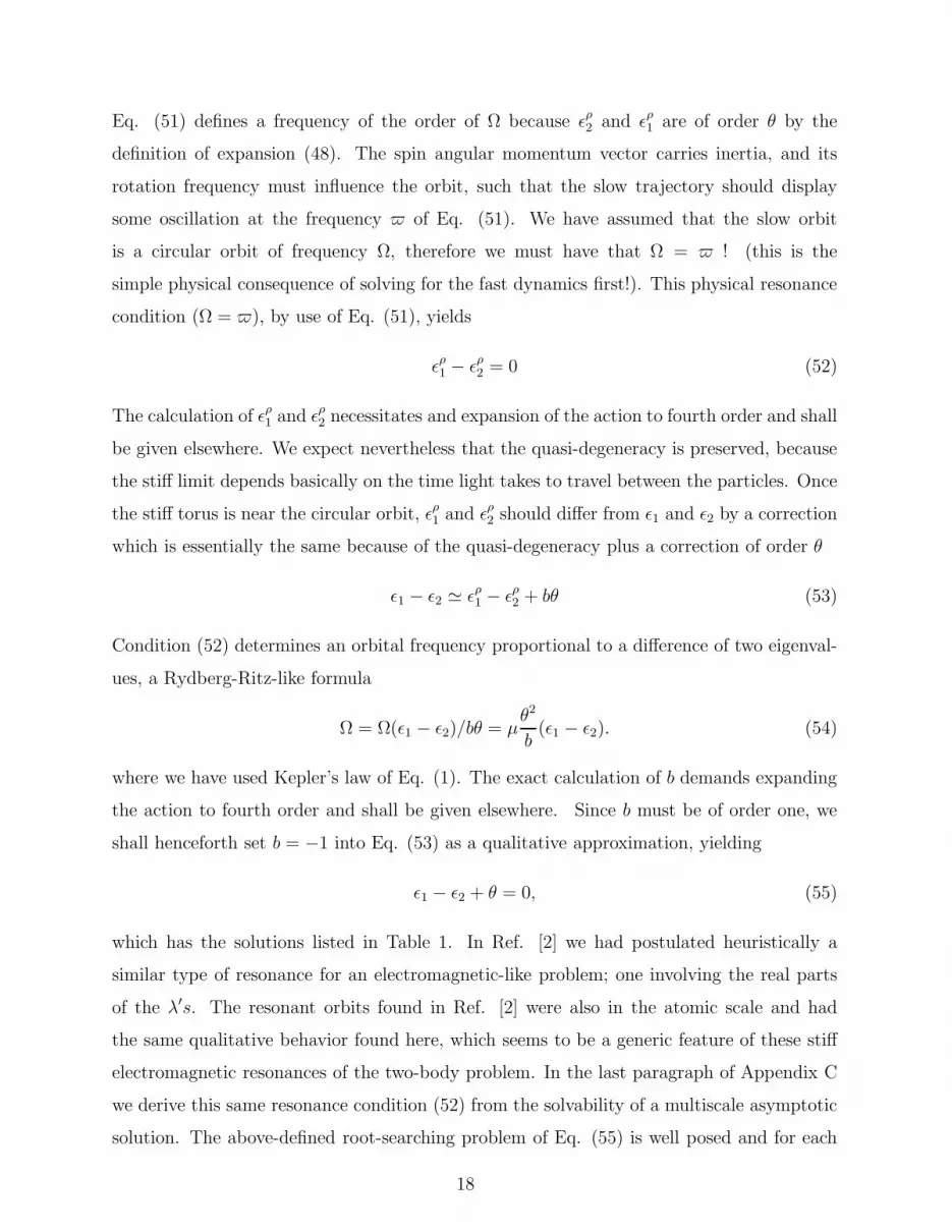
Eq. (51) defines a frequency of the order of Ω because ǫρ2 and ǫρ

1 are of order θ by the

definition of expansion (48). The spin angular momentum vector carries inertia, and its

rotation frequency must influence the orbit, such that the slow trajectory should display

some oscillation at the frequency of Eq. (51). We have assumed that the slow orbit

is a circular orbit of frequency Ω, therefore we must have that Ω = ! (this is the

simple physical consequence of solving for the fast dynamics first!). This physical resonance

condition (Ω = ), by use of Eq. (51), yields

ǫρ1 − ǫρ

2 = 0 (52)

The calculation of ǫρ1 and ǫρ

2 necessitates and expansion of the action to fourth order and shall

be given elsewhere. We expect nevertheless that the quasi-degeneracy is preserved, because

the stiff limit depends basically on the time light takes to travel between the particles. Once

the stiff torus is near the circular orbit, ǫρ1 and ǫρ

2 should differ from ǫ1 and ǫ2 by a correction

which is essentially the same because of the quasi-degeneracy plus a correction of order θ

ǫ1 − ǫ2 ≃ ǫρ1 − ǫρ

2 + bθ (53)

Condition (52) determines an orbital frequency proportional to a difference of two eigenval-

ues, a Rydberg-Ritz-like formula

Ω = Ω(ǫ1 − ǫ2)/bθ = µθ2

b(ǫ1 − ǫ2). (54)

where we have used Kepler’s law of Eq. (1). The exact calculation of b demands expanding

the action to fourth order and shall be given elsewhere. Since b must be of order one, we

shall henceforth set b = −1 into Eq. (53) as a qualitative approximation, yielding

ǫ1 − ǫ2 + θ = 0, (55)

which has the solutions listed in Table 1. In Ref. [2] we had postulated heuristically a

similar type of resonance for an electromagnetic-like problem; one involving the real parts

of the λ′s. The resonant orbits found in Ref. [2] were also in the atomic scale and had

the same qualitative behavior found here, which seems to be a generic feature of these stiff

electromagnetic resonances of the two-body problem. In the last paragraph of Appendix C

we derive this same resonance condition (52) from the solvability of a multiscale asymptotic

solution. The above-defined root-searching problem of Eq. (55) is well posed and for each

18

integer q it turns out that one can find a pair of the form (48) if one sacrifices θ in Eqs. (78)

and (45), i.e., θ must be quantized! According to QED, circular Bohr orbits have maximal

angular momenta and a radiative selection rule ( ∆l = ±1) restricts the decay from level

k + 1 to level k only, i.e., circular orbits emit the first line of each spectroscopic series

(Lyman, Balmer, Ritz-Paschen, Brackett, etc...), the third column of Table 1. We have

solved Eqs. (55) and Eqs. (78) and (45) with a Newton method in the complex λ-plane.

Every angular momentum 1/θ determined by Eq. (55) has the correct atomic magnitude.

These numerically calculated angular momenta θ−1 are given in Table 1, along with the

orbital frequency in atomic units (1373Ω)/µ = 1373θ2(ǫ2 − ǫ1), and the QED first frequency

of each spectroscopic series.

lz = θ−1 1373θ2(ǫ2 − ǫ1) wQED

185.99 3.996×10−1 3.750×10−1

307.63 8.831×10−1 6.944×10−2

475.08 2.398×10−2 2.430×10−2

577.99 1.331×10−2 1.125×10−2

694.77 7.667×10−3 6.111×10−3

826.22 4.558×10−3 3.685×10−3

973.12 2.790×10−3 2.406×10−3

1136.27 1.752×10−3 1.640×10−3

1316.44 1.127×10−3 1.173×10−3

1514.40 7.403×10−3 8.678×10−4

1730.93 4.958×10−3 6.600×10−4

1966.77 3.379×10−4 5.136×10−4

2222.70 2.341×10−4 4.076×10−4

q

7

9

11

12

13

14

15

16

17

18

19

20

21

Caption to Table 1: Numerically calculated angular momenta lz = θ−1 in units of e2/c,

orbital frequencies in atomic units (137θ)3 = 1373θ2(ǫ2−ǫ1), circular lines of QED in atomic

units wQED ≡ 12( 1

k2 − 1(k+1)2

) , and the values of the integer q of Eq. (48) and Eq. (49).

Table 1 illustrates the fact that a resonance involving the tangent dynamics of a circular

orbit predicts magnitudes in the atomic scale, as first discovered in Ref. [2]. In Ref. [2]

we had to jump the integer q by twenty units for a complete quantitative and qualitative

agreement with the Bohr atom. The qualitative agreement achieved by Table 1 is superior

19

in this way; only for the first two values of q things are not completely natural, and we had

to jump some q′s , after that q increases one by one in qualitative agreement with QED.

It remains to be seen if using the correct b given by the expansion about the stiff torus

will change things quantitatively. The calculation of b necessitates expanding the action to

fourth order and shall de done elsewhere.

VII. CONCLUSIONS AND DISCUSSION

In the limit where the proton has an infinite mass, the concept of resonant dissipation

looses meaning because the center-of-mass coordinate no longer plays a dynamical role.

In this singular limit, there is a Lorentz frame where the proton rests at the origin at all

times, and the field at the electron reduces to a simple Coulomb field in the ES. The two-

body dynamics in the ES reduces then to the dynamical system of Eliezer’s theorem; self-

interaction plus a Coulomb field acting on the electron [5, 6]. We repeat this correct dynamics

because it is very unpopular [5–8]; With inclusion of self-interaction, it is impossible for the

electron to ”spiral into the proton”. Neither bound states nor dives are possible, only

scattering states exist. One accomplishment of the present work is to recognize that only

the two-body problem can produce a physically sensible electromagnetic-like model. By

expanding the dynamics about a quasi-planetary orbit (the circular orbit), we saw the need

for a novel ingredient of the electromagnetic two-body dynamics; the stiff spinning motions!

Another qualitative dynamical picture is suggested by Eliezer’s result [5, 6]; The dynam-

ical phenomenon that the electron always turns away from the proton along unidimensional

orbits suggests that colinear orbits are the natural attractors of the dissipative dynamics

(the ground state of the hydrogen atom, with zero angular momentum!). Along such orbits,

the heavy particle (the proton) moves in a non-Coulombian way and the self-interaction

provides the repulsive mechanism that avoids the collision at the origin. This is again in

agreement with the Schroedinger theory, where the ground state has a zero angular mo-

mentum. Again, the infinite-mass case produces unphysical dynamics; the electron turns

away from the proton but then it runs away [6]. It remains to be researched if the two-body

version of Eliezer’s problem has a physical orbit among its zero-angular momentum orbits,

by taking proper care of the delay and its associated fast dynamics.

20

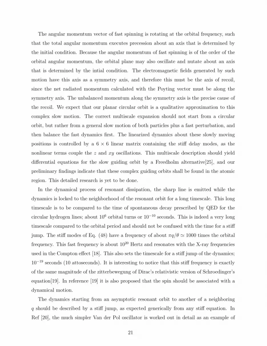
The angular momentum vector of fast spinning is rotating at the orbital frequency, such

that the total angular momentum executes precession about an axis that is determined by

the initial condition. Because the angular momentum of fast spinning is of the order of the

orbital angular momentum, the orbital plane may also oscillate and nutate about an axis

that is determined by the intial condition. The electromagnetic fields generated by such

motion have this axis as a symmetry axis, and therefore this must be the axis of recoil,

since the net radiated momentum calculated with the Poyting vector must be along the

symmetry axis. The unbalanced momentum along the symmetry axis is the precise cause of

the recoil. We expect that our planar circular orbit is a qualitative approximation to this

complex slow motion. The correct multiscale expansion should not start from a circular

orbit, but rather from a general slow motion of both particles plus a fast perturbation, and

then balance the fast dynamics first. The linearized dynamics about these slowly moving

positions is controlled by a 6 × 6 linear matrix containing the stiff delay modes, as the

nonlinear terms couple the z and xy oscillations. This multiscale description should yield

differential equations for the slow guiding orbit by a Freedholm alternative[25], and our

preliminary findings indicate that these complex guiding orbits shall be found in the atomic

region. This detailed research is yet to be done.

In the dynamical process of resonant dissipation, the sharp line is emitted while the

dynamics is locked to the neighborhood of the resonant orbit for a long timescale. This long

timescale is to be compared to the time of spontaneous decay prescribed by QED for the

circular hydrogen lines; about 106 orbital turns or 10−10 seconds. This is indeed a very long

timescale compared to the orbital period and should not be confused with the time for a stiff

jump. The stiff modes of Eq. (48) have a frequency of about πq/θ ≃ 1000 times the orbital

frequency. This fast frequency is about 1020 Hertz and resonates with the X-ray frequencies

used in the Compton effect [18]. This also sets the timescale for a stiff jump of the dynamics;

10−19 seconds (10 attoseconds). It is interesting to notice that this stiff frequency is exactly

of the same magnitude of the zitterbewegung of Dirac’s relativistic version of Schroedinger’s

equation[19]. In reference [19] it is also proposed that the spin should be associated with a

dynamical motion.

The dynamics starting from an asymptotic resonant orbit to another of a neighboring

q should be described by a stiff jump, as expected generically from any stiff equation. In

Ref [20], the much simpler Van der Pol oscillator is worked out in detail as an example of

21

an equation of Lienard type that exhibits stiff jumps. It is popular to use the concept of

a quantum jump to describe the stiff passage from one quantum state to another, but the

fact that classical electrodynamics prescribes exactly this qualitative phenomenon is news.

This quasi-instantaneous fast dynamics could be calculated theoretically and compared to

experiment.

The two-body dynamics in the ES solves several conundrums of the hydrogen atom. Most

of those conundrums were created by imagining that the equations of electrodynamics would

accept nonstiff planetary-like orbits. We have seen that the stiff spinning is necessary if a

balance of the fast dynamics is to be achived in the neighborhood of quasi-planetary orbits,

as proved by the Lemma of resonant dissipation of Appendix C. The balanced stiff spinning

is a novel and non-planetary feature that introduces a gyroscopic torque in the dynamics.

The qualitative agreements with QED are listed in the following; (i) the resonant orbits are

naturally quantized by integers and the radiated frequencies agree with the Bohr circular

lines within a few percent average deviation. (ii) the angular momenta of the resonant orbits

are naturally quantized with the correct Planck’s constant. (iii) the stability analysis near

the balanced stiff torus defines a linear dynamical system with delay, a dynamical system

that needs an initial function as the initial condition, just like Schroedinger’s equation. It

remains to be seen if this linear operator produces a self-adjoint Freedholm alternative[25],

like in Schroedinger’s equation. (iv) The emitted frequencies are given by a difference of two

eigenvalues of this linear operator, like the Rydberg-Ritz combinatorial principle of quantum

physics. (v) the spin angular momentum of the fast toroidal motion is of the order of the

lowest orbital angular momentum. The spin that we estimate is still a bit too high for QED,

where the electron has a spin angular momentum of√

3~/2 , and perhaps the full equations

can cure this[26, 27]. The calculation of the spin angular momentum for the balanced stiff

dynamics involves a detailed consideration of all stiff terms and is beyond the estimates of

the present work.

We exhibited a new solution of two-body motion in Dirac’s electrodynamics of point

charges. The stiff dynamics appears naturally in the two-body dynamics because of the

delay, and it has been so far overlooked. The balancing of the fast dynamics leads naturally

to fast spinning motions; the multiscale analysis imposes resonances, and these turn out to be

satisfied precisely in the atomic magnitude! The large body of qualitative and quantitative

agreement with QED suggests that further extensive studies of this two-body dynamics [4]

22

could offer an explanation of QED in terms of a stiff dynamical system with third derivatives

and delay.

VIII. ACKNOWLEDGEMENTS:

I thank Reginaldo Napolitano and Savio B. Rodrigues for discussions.

IX. APPENDIX A: ELIEZER’S ELECTRODYNAMICS OF POINT CHARGES

In Eliezer’s generalized electrodynamics[4], the field produced by the point charge is

supposed to be the retarded field plus a free field G

F νµ = F ν

µ,ret + Gνµ. (56)

The free field G should satisfy Maxwell’s equations, be finite along the particle’s worldline

and vanish if the particle is at rest. The choice of Eliezer in [4] is

Gνµ = k(F ν

µ,ret − F νµ,avd), (57)

where k is a fundamental parameter of nature related to the covariant limit producing the

point charge [4]. This generalized electromagnetic setting is henceforth called the Eliezer

setting (ES). Analogously to Dirac’s theory [1], Eliezer’s self-interaction is given by the

sourceless combination of half of the retarded Lienard-Wiechert self-potential minus half

of the advanced Lienard-Wiechert self-potential, but multiplied by a renormalizing factor

of (1 + 2k). This gives the following concise description of the ES; Charges interact with

themselves via the semi-difference of Lienard-Wiechert self-potentials and with other charges

via a linear combination of Lienard-Wiechert potentials. In Eliezer’s theory the electron and

the proton of a hydrogen atom have the following equations of motion [4]

m1v1µ − 2

3(1 + 2k)[v1µ − ||v1||2v1µ] = −[F ν

µ,in + (1 + k)F νµ2,ret − kF ν

µ2,advt]v1ν , (58)

m2v2µ − 2

3(1 + 2k)[v2µ − ||v2||2v2µ] = [F ν

µ,in + (1 + k)F νµ1,ret − kF ν

µ1,adv]v2ν ,

where viµ stands for the quadrivelocity of particle i, double bars stand for the Minkowski

scalar product and the dot represents derivative respect to the proper time of each particle.

23

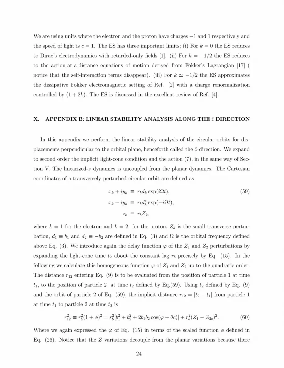
We are using units where the electron and the proton have charges −1 and 1 respectively and

the speed of light is c = 1. The ES has three important limits; (i) For k = 0 the ES reduces

to Dirac’s electrodynamics with retarded-only fields [1]. (ii) For k = −1/2 the ES reduces

to the action-at-a-distance equations of motion derived from Fokker’s Lagrangian [17] (

notice that the self-interaction terms disappear). (iii) For k ≃ −1/2 the ES approximates

the dissipative Fokker electromagnetic setting of Ref. [2] with a charge renormalization

controlled by (1 + 2k). The ES is discussed in the excellent review of Ref. [4].

X. APPENDIX B: LINEAR STABILITY ANALYSIS ALONG THE z DIRECTION

In this appendix we perform the linear stability analysis of the circular orbits for dis-

placements perpendicular to the orbital plane, henceforth called the z-direction. We expand

to second order the implicit light-cone condition and the action (7), in the same way of Sec-

tion V. The linearized-z dynamics is uncoupled from the planar dynamics. The Cartesian

coordinates of a transversely perturbed circular orbit are defined as

xk + iyk ≡ rbdk exp(iΩt), (59)

xk − iyk ≡ rbd∗

k exp(−iΩt),

zk ≡ rbZk,

where k = 1 for the electron and k = 2 for the proton, Zk is the small transverse pertur-

bation, d1 ≡ b1 and d2 ≡ −b2 are defined in Eq. (3) and Ω is the orbital frequency defined

above Eq. (3). We introduce again the delay function ϕ of the Z1 and Z2 perturbations by

expanding the light-cone time t2 about the constant lag rb precisely by Eq. (15). In the

following we calculate this homogeneous function ϕ of Z1 and Z2 up to the quadratic order.

The distance r12 entering Eq. (9) is to be evaluated from the position of particle 1 at time

t1, to the position of particle 2 at time t2 defined by Eq.(59). Using t2 defined by Eq. (9)

and the orbit of particle 2 of Eq. (59), the implicit distance r12 = |t2 − t1| from particle 1

at time t1 to particle 2 at time t2 is

r212 ≡ r2

b (1 + φ)2 = r2b [b

21 + b2

2 + 2b1b2 cos(ϕ + θc)] + r2b (Z1 − Z2c)

2. (60)

Where we again expressed the ϕ of Eq. (15) in terms of the scaled function φ defined in

Eq. (26). Notice that the Z variations decouple from the planar variations because there

24

is no mixed linear term of Z times a linear perturbation of the planar coordinate in Eq.

(60); terms in Z only appear squared. Expanding Eq. (60) up to the second order and

rearranging yields

φ2 + 2Sφ = (Z1 − Z2c)2 (61)

a quadratic equation for φ with the regular solution correct to second order given by

φ =1

2S(Z1 − Z2c)

2. (62)

The coordinate Z2 appears evaluated at the advanced/retarded time in Eq. (62), and to

obtain the action up to quadratic terms it is sufficient to keep the first term Z2(τ 1 + cθ +ϕ)

≃ Z2(τ 1 + cθ) ≡ Z2c. Using the z−perturbed orbit defined by Eq. (59) to calculate the

numerator of the VA interaction of Eq. (8) yields

(1 − v1 · v2c) = 1 + θ2 cos(θ + cϕ)b1b2 − θ2Z1Z2c ≈ (63)

C − θ2(S − 1)φ − θ2Z1Z2c,

and the denominator of the VA interaction of Eq. (8) is

r12(1 + n12c · v2c/c) = rb[1 + φ + θcb1b2 sin(θc + ϕc) + θc(Z1 − Z2c)Z2c]. (64)

Notice that the quadratic term Z2cZ2c on the right-hand side of Eq. (64) can be dropped

because it represents an exact Gauge that does not affect the Euler-Lagrange equations of

motion. We also expand the argument of the sign function of the right-hand side of Eq. (64)

until the linear term in ϕc, such that the quadratic approximation to Eq. (64) is

r12(1 + n12c · v2c/c) ≈ rb[S + Cφ + θcZ1Z2c], (65)

where the equivalence sign ≈ henceforth means equivalent up to a Gauge term of second

order. Even if a quadratic Gauge term appears in the denominator, in an expansion up to

quadratic order it would still produce a Gauge and therefore it can be dropped directly from

the denominator. In this way, the expansion up to second order of the VA interaction of Eq.

(7) is simply

Θ ≈ (C

rbS)(1 + k)[1 − θ2CS2Z1Z2− − C2S

2(Z1 − Z2−)2 + θC2SZ1Z2−] (66)

−k[1 − θ2CS2Z1Z2+ − C2S

2(Z1 − Z2+)2 − θC2SZ1Z2+].

25

Last, we need the kinetic energy along the z-perturbed circular orbit, which we express in

terms of Z1 of definition (59) as

T1 = −m1

√

1 − v21 = −m1

γ1

√

1 − γ21θ

2Z21 , (67)

where the dot means derivative with respect to the scaled time τ , γ−11 ≡

√

1 − v21 , and we

have used Ωrb = θ. The expansion of Eq. (67) up to second order is

T1 = (1

rb)−rbm1

γ1

+ǫ1

2Z2

1 + ..., (68)

where ǫ1 ≡ m1rbγ1θ2 = r3

bm1γ1Ω2. The Euler-Lagrange equation of motion for particle 1 of

the isolated two-body problem is determined from the quadratic Lagrangian

L1 = T1 + Θ. (69)

We shall henceforth disregard the small corrections to the quadratic coefficients and use

C = 1, S = 1 , which is the stiff-limit. The equation of motion for particle 1 is

ǫ1Z1 = −[Z1 − (1 + k)Z2− + kZ2+] + θ[kZ2+ + (1 + k)Z2−) + θ2[kZ2+ − (1 + k)Z2−]. (70)

Notice that the term on the left-hand side of Eq. (70) can be written as

ǫ1Z1 = r3bm1γ1Ω

2Z1 = r2b

dpz

dt, (71)

which is proportional to the force along the z-direction multiplied by the factor r2b . According

to the equation of motion of the ES (see appendix A), we must add the following self-

interaction term to the right-hand side of Eq. (70)

r2bFrad =

2

3(1 + 2k)θ3...

Z 1, (72)

where the triple dot means three derivatives with respect to the scaled time and we have

used Eq. (10). The full linearized equation of motion for Z1 is

ǫ1Z1 =2

3(1 + 2k)θ3...

Z1 − [Z1 + kZ2+ − (1 + k)Z2−] (73)

+θ[kZ2+ + (1 + k)Z2−] + θ2[kZ2+ − (1 + k)Z2−].

The linearized equation for Z2 is completely analogous and is obtained by interchanging

Z1 by Z2 and ǫ1 by ǫ2 in Eq. (73). (Comparing Eq. (73) to Eq. (30) of Ref. [2] we find that

26

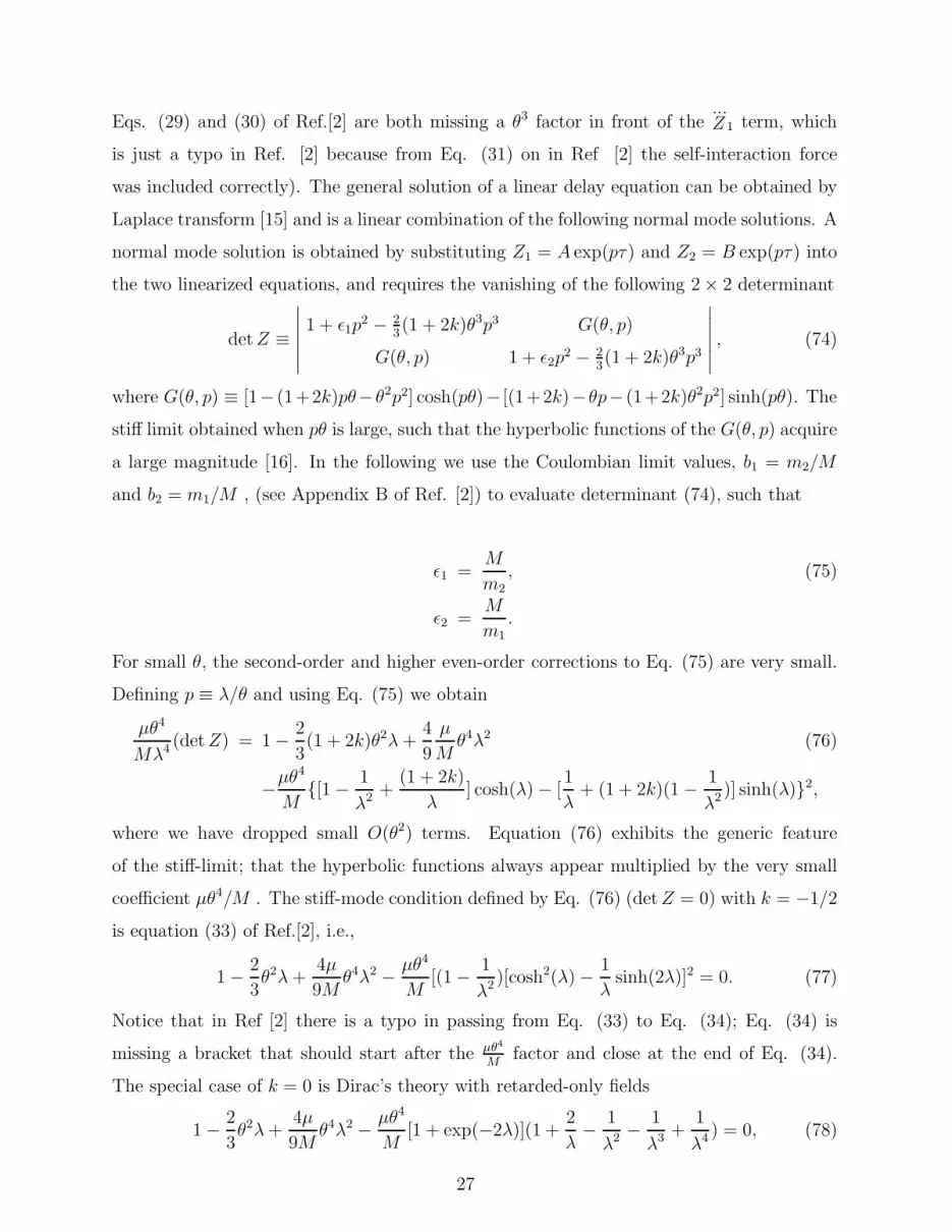
Eqs. (29) and (30) of Ref.[2] are both missing a θ3 factor in front of the...Z 1 term, which

is just a typo in Ref. [2] because from Eq. (31) on in Ref [2] the self-interaction force

was included correctly). The general solution of a linear delay equation can be obtained by

Laplace transform [15] and is a linear combination of the following normal mode solutions. A

normal mode solution is obtained by substituting Z1 = A exp(pτ) and Z2 = B exp(pτ) into

the two linearized equations, and requires the vanishing of the following 2 × 2 determinant

det Z ≡

∣

∣

∣

∣

∣

∣

1 + ǫ1p2 − 2

3(1 + 2k)θ3p3 G(θ, p)

G(θ, p) 1 + ǫ2p2 − 2

3(1 + 2k)θ3p3

∣

∣

∣

∣

∣

∣

, (74)

where G(θ, p) ≡ [1− (1+2k)pθ−θ2p2] cosh(pθ)− [(1+2k)−θp− (1+2k)θ2p2] sinh(pθ). The

stiff limit obtained when pθ is large, such that the hyperbolic functions of the G(θ, p) acquire

a large magnitude [16]. In the following we use the Coulombian limit values, b1 = m2/M

and b2 = m1/M , (see Appendix B of Ref. [2]) to evaluate determinant (74), such that

ǫ1 =M

m2

, (75)

ǫ2 =M

m1.

For small θ, the second-order and higher even-order corrections to Eq. (75) are very small.

Defining p ≡ λ/θ and using Eq. (75) we obtain

µθ4

Mλ4 (det Z) = 1 − 2

3(1 + 2k)θ2λ +

4

9

µ

Mθ4λ2 (76)

−µθ4

M[1 − 1

λ2 +(1 + 2k)

λ] cosh(λ) − [

1

λ+ (1 + 2k)(1 − 1

λ2 )] sinh(λ)2,

where we have dropped small O(θ2) terms. Equation (76) exhibits the generic feature

of the stiff-limit; that the hyperbolic functions always appear multiplied by the very small

coefficient µθ4/M . The stiff-mode condition defined by Eq. (76) (det Z = 0) with k = −1/2

is equation (33) of Ref.[2], i.e.,

1 − 2

3θ2λ +

4µ

9Mθ4λ2 − µθ4

M[(1 − 1

λ2 )[cosh2(λ) − 1

λsinh(2λ)]2 = 0. (77)

Notice that in Ref [2] there is a typo in passing from Eq. (33) to Eq. (34); Eq. (34) is

missing a bracket that should start after the µθ4

Mfactor and close at the end of Eq. (34).

The special case of k = 0 is Dirac’s theory with retarded-only fields

1 − 2

3θ2λ +

4µ

9Mθ4λ2 − µθ4

M[1 + exp(−2λ)](1 +

2

λ− 1

λ2 − 1

λ3 +1

λ4 ) = 0, (78)

27

where the appearance of the negative exponential only is related to the retardation-only, in-

stead of the hyperbolic functions related to advanced and retarded interactions. Comparing

Eq. (76) to Eq. (44) we can see that the phenomenon of quasi-degeneracy exists only for

k = 0 (Dirac’s theory) and for k = −1/2 (the action-at-a-distance electrodynamics and the

dissipative Fokker theory of Ref. [2]).

XI. APPENDIX C: LEMMA OF RESONANT DISSIPATION

Substituting the circular orbit into the equations of motion, Eqs. (58), one finds at

leading order for the electronic motion an offending term described by a force opposite to

the electronic velocity

r2bF1 = r2

b

2

3

...x 1 = −2e2

3c3Ω2r2

b x1 = −2

3θ3. (79)

where we have included the scaling factor r2b as of Eq. (72). Along the trajectory of the

proton, the delayed Lienard-Wiechert interaction with the electron is the main offending

force against the velocity, instead of the much smaller protonic self-interaction. Using the

Page series in the same way of Ref. [13], we find a force against the protonic velocity of the

same magnitude of Eq.(79), as illustrated in Fig. 2. These offending forces destabilize the

unperturbed circular motion with a small torque and a slow dissipation. In quantum elec-

trodynamics (QED) the circular Bohr orbits[3] of hydrogen correspond to excited states that

decay to the ground state in a life-time of about 106 turns. Using Eq. (79) to estimate the

energy dissipation along circular orbits of the atomic magnitude, one finds a net dissipation

of about 4 electron-volts after the life-time of 106 turns, an order-one fraction of the biding

energy (13.6 electron-volts). This radiative instability in the slow timescale is an incomplete

picture of the dynamics because it disregards the fast stiff motion that is present because

of the delay. Let us postulate heuristically that along some special circular orbits the fast

dynamics encircles the circular orbit as illustrated in Fig. 1. If the linearization about the

circular orbit, Eq. (49), is averaged over a timescale of some turns, the stiff dynamics goes

away and the resulting variable is a slow moving drift (representing the recoil of the state

28

of resonant dissipation). For that slow motion we have

ξ1(τ ) = ξ1+(τ) = ξ1−(τ ), (80)

ξ2(τ ) = ξ2+(τ) = ξ2−(τ ),

since we are averaging the argument over a time of many turns, a time much longer than

the delay θ. We are ready to prove that the dynamics of the state of resonant dissipation

must necessarily involve a nonlinear term of the expansion about a circular orbit.

Lemma: If the averaged dynamics is determined only by the linear terms plus the offend-

ing forcing, the state of resonant dissipation is impossible. To show this we average the full

equation of motion of the ξ1 variable, which is

⟨

2θ3

3(...u 1 + ib1)

⟩

+ l1ξ − ib1θ3 + NL = 0, (81)

where the term inside brackets is the average of the linearized correction to the self-

interaction force, l1ξ stands for the average of Eq. (41) and NL stands for the average

of the nonlinear terms. The time averages of the term inside brackets and of the first and

second derivatives in Eq. (41) are zero, such that discarding the nonlinear term of Eq. (81)

yields the non-homogeneous linear equation

−(N11 + θ2G)ξ1 − (M1 + U11)η1 (82)

−(R∗

+ + R∗

−)ξ2 − (P+ + P−)η2

= ib1θ3.

Performing the same average for the other three coordinates, we obtain a system of four

non-homogeneous linear equations. The matrix of this linear system has a zero determinant

that is directly related to the Galilean translation mode of the circular orbit, such that it

defines a singular linear operator. Moreover, the forcing term turns out to be out of the

image of the singular linear operator, such that the linear system has no solution at all! This

completes the proof of our lemma.

Last, we mention a derivation of Eq. (52) from the equations of motion in the form (81);

This can be accomplished by placing the linearization about the stiff torus on the left-hand

side (henceforth called the Kernel) and the forcing and nonlinear terms on the right-hand

side. In this way the right-hand side has to be orthogonal to the left-eigenvectors of the

29

Kernel, which is the Freedholm alternative theorem discussed for example in Refs. [24, 25].

Multiplying the Kernel by a left-eigenvector and integrating on the fast timescale has exactly

the form of the conservation law for angular momentum on the slow time scale. This shall

be studied elsewhere.

XII. APPENDIX D: HARMONIC SOLUTION AND SPINORIAL UNFOLDING

The lemma of resonant dissipation of Appendix C suggests the participation of the nonlin-

ear terms to achieve the state of resonant dissipation of Fig. 1. We shall see in the following

that because of the fast frequency in the stiff terms, even at small amplitudes the nonlinear

stiff terms give a large contribution to the self-force. Our perturbation scheme started from

a guiding circular orbit that is not a solution to the equations of motion, because of the

offending force of Eq. (79). In the following we show how to balance this offending force

at a small distance away from the circular orbit. The full Lorentz-Dirac self-force is given

in page 116 of Ref [22], expressed in terms of the Cartesian velocity of the particle, v1, its

acceleration a1 and its second acceleration a1 respectively. This full self-force multiplied by

the convenient scaling factor of Eq. (72) is

r2bF1 =

2

3γ3

1r2ba1 + 3γ2(v1 · a1)a1 + γ2

1[(v1 · a1) + 3γ21(v1 · a1)

2]v1. (83)

Assuming that the particle coordinates are described by a slow term plus a fast term, Eq.

(49), we use Eq. (83) as follows; We estimate each coefficient of the v1, a1 and a1 terms by

substituting the fast component of the trajectory, Eq. (49), and taking the time average. For

the estimate below, the vectors v1, a1 and a1 are replaced by the slow quantities evaluated

along the unperturbed orbit. For example the coefficient of the velocity term in Eq. (83)

(r2b times the term inside the square brackets on the right-hand side of Eq. (83) ) is

r2bγ

21[(v1 · a1) + 3γ2

1(v1 · a1)2] = γ2

1|λ|4ρ2(3γ21|λ|2ρ2 − 1) (84)

Notice that for a large enough ρ there is a critical value where this coefficient changes sign,

or

3γ21|λ|2ρ2 > 1, (85)

We show in the following that the value of ρ1 must be very near this critical value. The

self-forces for the electron and proton, both measured along the direction of the electronic

30

velocity, are

r2bF1 =

2

3[−θ3b1 + γ2

1|λ|4ρ21(3γ

21|λ|2ρ2

1 − 1)θb1], (86)

r2bF2 =

2

3[θ3b2 − γ2

2|λ|4ρ22(3γ

22|λ|2ρ2

2 − 1)θb2], (87)

where b1 and b2 are given by Eq. (3). In the state of resonant dissipation, the relative

separation of the particles executes a circular motion, such that the tangential force must

vanish

b1F1 − b2F2 = 0, (88)

with b1 = m2/(m1 + m2) and b2 = m1/(m1 + m2). Because b2 ≪ 1 we can disregard the

protonic contribution such that Eq. (88) yields

ρ1 =

√

1

3|λ|2 (1 +θ2

|λ|4ρ21

) ≃ 1√

3|λ|2. (89)

This distance is a few percent of the orbital radius, and it is some 500 classical electronic

radia for θ in the atomic scale. The spin angular momentum of the electron calculated by

Eq. (50) is |l| ∼ 1/(6πqθ2), which is of the order of the orbital angular momentum.

The nonlinear correction to Eq. (78) can be estimated by taking into account the non-

linear terms of the Lorentz-Dirac self-force. This correction to Eq. (78), estimated along

a harmonic solution for the averaged equations of tangent dynamics, in a way explained

above, yields

(1 +2

λz

− 1

λ2z

− 1

λ3z

+1

λ4z

+ ...)(µθ4

M) exp(−2λz) (90)

= 1 − 2ρ2|λ|3 − 2

3θ2λz +

4µ

Mθ4λ2

z + ...,

Because of the extra term on the right-hand side of Eq. (90), a harmonic solution to the

nonlinear equations of tangent dynamics exists if

ρ ≃ 1√2|λ|3/2

. (91)

The fact that the two necessary and independent estimates (89) and (91) agree suggests

that the stiff torus of Fig. 1 is a solution of Dirac’s equations of motion[1] for the two-

body problem! In summary, our perturbative scheme shows that the stiff torus of Fig. 2

31

is a solution to the equations of motion as follows; (i) We expand about a circular orbit

and calculate the radius of the stiff torus by the condition that a harmonic solution to the

nonlinear equations of tangent dynamics exists (Eq. 91). (ii) This balanced stiff spinning

about the circular orbit cancels the offending force of Eq. (79), predicting a radius by (89)

that is in agreement with the radius of (91). (iii) Resonance condition (52) is a necessary

condition for the existence of an asymptotic expansion of the dynamics about the stiff torus,

i.e., the condition for a smooth recoil of the atom as a bound state. The detailed unfolding of

the equations of tangent dynamics is beyond the estimates of this Appendix and necessitates

the full nonlinear equations.

XIII. CAPTIONS

Fig. 1: The guiding-center circular orbit of each particle is illustrated by dashed lines.

Particle trajectories are the stiff tori gyrating about the guiding-center circular orbit of each

particle (dark solid lines). Illustrative purposes only, the radia are not on scale. Arbitrary

units.

Fig. 2: The unperturbed circular orbit with the particles in diametral opposition at the

same time in the inertial frame. Indicated is also the advanced position of particle 1 and the

angle travelled during the light-cone time. The drawing is not on scale; The circular orbit

of the proton has an exaggerated radius for illustrative purposes. Arbitrary units.

[1] P. A. M.Dirac, Proceedings of the Royal Society of London, ser. A 167,148 (1938).

[2] J. De Luca, Physical Review E , 71 056210 (2005).

[3] N. Bohr, Philos. Mag., 26, 1 (1913); 26, 476 (1913).

[4] C. Jayaratnam Eliezer, Reviews of Modern Physics, 19 (1947).

[5] C.J. Eliezer, Proc. Cambridge Philos. Soc. 39, 173 (1943).

[6] S. Parrott, Foundations of Physics 23, 1093 (1993).

[7] A. Carati, J. Phys. A: Math. Gen. 34, 5937 (2001).

[8] M. Marino, J. Phys. A: Math. Gen 36, 11247 (2003).

32

[9] A. Schild, Phys. Rev. 131 2762 (1963); A. Schild, Science 138 994 (1962).

[10] M. Schonberg, Phys. Rev. 69, 211 (1946).

[11] J. L. Anderson, Principles of Relativity Physics , Academic press, New York (1967), page 225.

[12] L. Page, Physical Review 24, 296 (1924).

[13] J. De Luca, Phys. Rev. Lett. 80, 680 (1998) .

[14] C. M. Andersen and H. C. von Baeyer, Phys. Rev. D 5, 802 (1972).

[15] R. E. Bellman and K.L.Cooke, Differential-Difference Equations, Academic Press, New York

(1963), page 393.

[16] A. Staruszkiewicz, Acta Physica Polonica, XXXIII, 1007 (1968).

[17] J. A. Wheeler and R. P. Feynman, Rev. Mod. Phys. 17, 157 (1945); J. A. Wheeler and R. P.

Feynman, Rev. Mod. Phys. 21, 425 (1949).

[18] J. N. Dodd, Eur. J. Phys. 4, 205 (1983).

[19] D. Hestenes, Am. J. Phys. 47, 399 (1979), D. Hestenes, Foundations of Physics 15, 63 (1983).

[20] J. Grasman, Asymptotic Methods for Relaxation Oscillations and Applications, Applied Math-

ematical Sciences , 63, Springer-Verlag, New-York (1987).

[21] J. De Luca, to be published.

[22] F. Rohrlich, Classical Charged Particles Addison-Wesley Publishing, NY (1965).

[23] J. De Luca, Phys. Rev. E 62, 2060 (2000).

[24] J. De Luca , R. Napolitano and V. Bagnato, Physical Review A, 55 R1597 (1997), J. De Luca,

R. Napolitano and V. Bagnato, Physics Letters A 233 79 (1997).

[25] J. Mallet-Paret, Journal of Dynamics and Differential Equations 11, 1 (1999).

[26] W. Appel and M. K.-H.Kiessling, Annals of Physics (NY) 289, 24 (2001)

[27] Sin-itiro Tomonaga, Translated by Takeshi Oka, The story of spin The University of Chicago

Press, Ltd., London (1997).

33