saturated aquifer reservoirs using surface geophysical methods

1112 The Leading Edge October 2011

P e t r o p h y s i c sP e t r o p h y s i c s

The process of capturing carbon dioxide (CO2) and injecting it into deep saline aquifers is becoming an

important method to reduce future atmospheric emissions of CO2. Key challenges facing carbon capture and storage (CCS) are the storage reservoir’s size and safety. The storage size can be addressed by focusing on large saline aquifer reservoirs. The safety concern may be lower if CO2 is injected into depleted hydrocarbon reservoirs because their cap-rock integrity is already proven, but such capping systems are generally potentially compromised by poorly cemented abandoned wells, and compared to saline aquifers, their storage size is small. Therefore, the long-term focus of CCS is on saline aquifers. To reduce the corresponding risks, comprehensive long-term monitoring is inevitable.

Monitoring stored CO2 is fundamental to the operation and management of the storage site. To monitor a given CO2 store, we must be able to observe and track any changes in the subsurface distribution of CO2 during injection, post-injection site management, and post-closure stewardship. Monitorability of a site is a major source of uncertainty that should be quantified prior to injection of CO2. If secure stor-age cannot be verified via geophysical monitoring, it is not likely a viable candidate for carbon capture and storage.

The suite of monitoring techniques employed should at least be able to detect where some minimum threshold com-bination of volume and saturation of CO2 has been exceeded within a subsurface reservoir or after leakage into the over-burden. Moreover, the saturation (and hence volume) of CO2 must be estimable within some predefined or characteristic spatial volume, with some minimum degree of accuracy. De-fining these minimum thresholds is equivalent to defining the term “monitorable.” No standard definition of what is required for a site to be monitorable has been agreed upon to date; because CO2 detectability is a necessary condition for monitorability, this work contributes necessary information toward that definition.

The detectability assessment approach presented in this paper is particularly useful at early stages of site selection and associated decision making in which a cost-efficient yet comprehensive estimate of the site monitorability is required. Early stages are plagued by lack of detailed information about key reservoir and overburden petrophysical properties, par-ticularly in aquifer sites. These assessments of detectability, and more generally monitorability, must account for such uncertainty. Although there is a range of geophysical moni-toring techniques which are finding greater application (e.g., INSAR, tilt, passive seismics, well-based techniques, etc.), in this article we focus on the surface seismics, gravity, and controlled-source electromagnetic (CSEM) methods. We pay particular attention to offshore geophysical methods, but many of our conclusions are also valid for onshore monitor-ing.

ARASH JAFARGANDOMI and ANDREW CURTIS, University of Edinburgh

Petrophysical properties of CO2-bearing rocksPetrophysical model. Rock and fluid physics measurements and theoretical modeling show that the presence of CO2 af-fects the (an)elastic parameters, density, and electrical con-ductivity of the reservoir. In partially saturated rocks, the bulk modulus depends not only on the degree of saturation, but also on the mesoscopic and microscopic distribution of the fluids. “Patchy” saturation and uniform saturation are considered to be the two extreme cases of saturation style (Mavko et al., 1998). Whether one should use patchy or uni-form saturation to describe fluid heterogeneity depends on the monitoring frequency of interest. In reality, the observed intrinsic seismic-wave dispersion in sedimentary rocks is greater than that which can be explained by existing petro-physical models. Recent studies have shown that the intrinsic attenuation in porous media throughout the seismic band of frequencies (1–10,000 Hz) is mainly due to wave-induced fluid flow at the mesoscopic scale, larger than the pore but smaller than the wavelength (Pride et al., 2003). The meso-scopic-scale attenuation was first modeled by White (1975). In addition to the mesoscopic-scale attenuation, Biot and squirt flow are the other known mechanisms responsible for the wave attenuation in porous media at the higher frequen-cies.

We combine White’s model with the model developed by Pham et al. (2002) that contains both Biot and squirt-flow effects, by adjusting the matrix bulk modulus of the latter with the frequency-dependent bulk modulus of the former. The combined model takes into account all of the above-mentioned effects on the seismic waves.

To investigate the effect of CO2 saturation (SCO2) on the electrical resistivity (1/σ where σ is conductivity) of the reser-voir rocks, we use Archie’s model (Archie, 1942). To estimate the gravity response of the reservoir due to CO2 saturation, we calculate bulk density of the saturated rocks as a weighted superposition of densities of solid and fluid constituents.

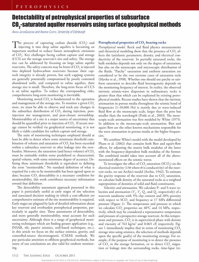
Velocities and attenuation. We calculate P- and S-wave ve-locities and attenuation (Vp, Vs, Qp, and Qs, respectively) of a reservoir sandstone with 5% clay content and 20% porosity with respect to SCO2 and frequency at 17 MPa differential pressure (Figure 1). The temperature and pressure in which we calculate CO2 properties are 40°C and 14 MPa, respec-tively, which may be considered a representative temperature and pressure of a prospective storage reservoir. At this temper-ature and pressure, CO2 is in supercritical phase with density and viscosity of 763 kg/m3 and 0.065 cP, respectively. Fig-ure 1 immediately implies that in terms of monitoring CO2 storage sites using seismics, the selection of methods depends upon the specific goal(s) of the monitoring strategy. For ex-ample, if the purpose of monitoring is to detect the presence of CO2 in the storage formation, or to detect CO2 migra-tion or leakage into the surrounding rocks, time-lapse (re-

Downloaded 18 Oct 2011 to 129.215.6.61. Redistribution subject to SEG license or copyright; see Terms of Use at http://segdl.org/

October 2011 The Leading Edge 1113

P e t r o p h y s i c s

peated) single-component (P-wave) reflection seismics with a low-frequency content may be sufficient because Vp will show significant changes even with a small amount of CO2 in the brine. However, if the purpose of monitoring is to evaluate the amount and spatial distribution of injected CO2 (i.e., to estimate SCO2 in the brine), low-frequency methods such as time-lapse reflection surface seismics may not be appropri-ate because their sensitivity is minimal to saturations beyond approximately 10–20%; higher frequency techniques such as sonic logging or crosswell methods may have to be applied because, at these frequencies, seismic Vp estimates are more sensitive to changes in higher saturations than low-frequency methods. Nevertheless, in most injection scenarios one may expect up to ~5% CO2 dissolved in brine, in which case sur-face seismic methods may well suffice.

In contrast to the Vp sensitivities, Vs presents low sensitiv-ity to both frequency and SCO2 and may not be an appro-priate parameter to estimate for monitoring CO2 presence, migration, or saturation. However, the slight increase in Vs with CO2 saturation contributes to decreased Poisson’s ratio. Also, sensitivity of Vs to changes in elastic parameters of the rock matrix makes it an appropriate parameter to measure to monitor the cap-rock integrity. This is particularly the case because anisotropy of Vs has been shown to be highly sensi-tive to bulk changes in fracture properties. Time-lapse mea-surement of Vs may also be used to identify the changes in the reservoir porosity due to the pore fluid pressure increase and chemical interaction between the brine-CO2 mixture and the rock matrix.

Variation of attenuation with respect to SCO2 and frequen-cy is more complicated than that of the wave velocities. Figure 1b shows a large peak at low frequencies corresponding to the mesoscopic-scale wave-induced fluid flow. This peak is larger than the Biot and squirt-flow peaks at higher frequencies which makes attenuation an appropriate parameter to monitor, if it can be estimated accurately. S-wave attenuation is not sensitive

to SCO2 at low frequency; however, at intermediate and higher frequencies, it is sensitive to SCO2 and can potentially be monitored with well-based seis-mic methods.

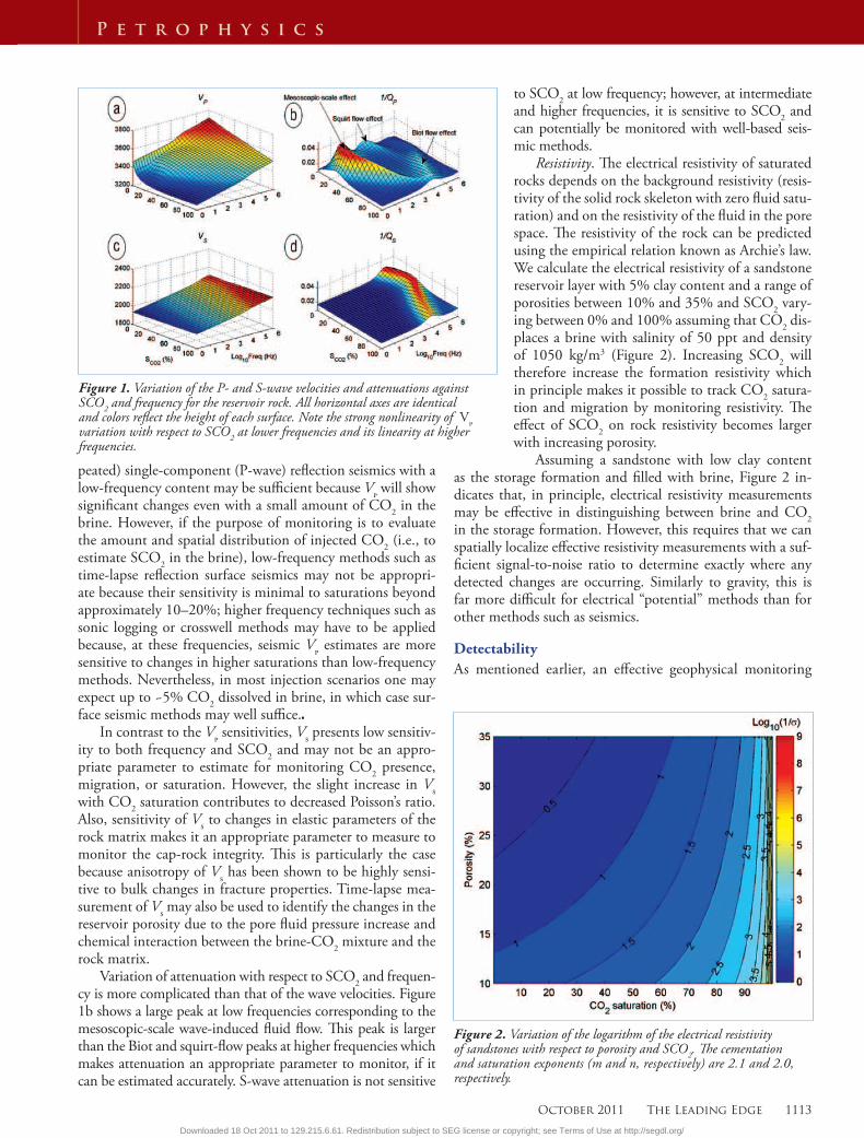
Resistivity. The electrical resistivity of saturated rocks depends on the background resistivity (resis-tivity of the solid rock skeleton with zero fluid satu-ration) and on the resistivity of the fluid in the pore space. The resistivity of the rock can be predicted using the empirical relation known as Archie’s law. We calculate the electrical resistivity of a sandstone reservoir layer with 5% clay content and a range of porosities between 10% and 35% and SCO2 vary-ing between 0% and 100% assuming that CO2 dis-places a brine with salinity of 50 ppt and density of 1050 kg/m3 (Figure 2). Increasing SCO2 will therefore increase the formation resistivity which in principle makes it possible to track CO2 satura-tion and migration by monitoring resistivity. The effect of SCO2 on rock resistivity becomes larger with increasing porosity.

Assuming a sandstone with low clay content as the storage formation and filled with brine, Figure 2 in-dicates that, in principle, electrical resistivity measurements may be effective in distinguishing between brine and CO2 in the storage formation. However, this requires that we can spatially localize effective resistivity measurements with a suf-ficient signal-to-noise ratio to determine exactly where any detected changes are occurring. Similarly to gravity, this is far more difficult for electrical “potential” methods than for other methods such as seismics.

DetectabilityAs mentioned earlier, an effective geophysical monitoring

Figure 1. Variation of the P- and S-wave velocities and attenuations against SCO2 and frequency for the reservoir rock. All horizontal axes are identical and colors reflect the height of each surface. Note the strong nonlinearity of Vp variation with respect to SCO2 at lower frequencies and its linearity at higher frequencies.

Figure 2. Variation of the logarithm of the electrical resistivity of sandstones with respect to porosity and SCO2. The cementation and saturation exponents (m and n, respectively) are 2.1 and 2.0, respectively.




method should at least be able to detect where some mini-mum threshold volume or saturation of CO2 has been ex-ceeded within the reservoir. Here, this minimum threshold is used to define the detectability. We define a set of diagnos-tic parameters for different geophysical methods (seismics, gravimetry, CSEM). Each is used to assess the detectability of changes in geophysical parameters of reservoir rocks due to increased SCO2. These changes are calculated by compar-ing geophysical responses of the reservoir before and after injecting CO2. We use the following general equation for the detectability parameters:

(1)

where X0 and X are values of geophysical parameters mea-sured with a particular geophysical method before and af-ter injecting CO2. Respectively, C is a parameter which may depend on some of the other parameters (defined in Table 1 for each method), and std(X) is the uncertainty or noise level (NL) which dictates the minimum required changes in geo-physical parameters to produce statistically distinguishable geophysical signals. Corresponding detectability parameters for the seismics, gravity, and CSEM methods are given in Table 1. Note that the detectability parameters in Table 1 are based on simplifying assumptions and are intended as a guide rather than an actual practical tool; however, for the type of analysis that we present in this paper (which is focused on the early stages of monitoring design with minimum avail-able information about the site) they seem satisfactory.

SeismicsAn important goal for geophysical monitoring of CO2 stor-

age in brine-saturated aquifers is the ability to discriminate between different saturating fluids. Techniques used in seismic analysis such as analyzing the AVO response have proven effective. To assess the detectability of CO2 in the reservoir with low-frequency seismic methods, we use the AVO detectability criterion presented by Dong (1999) (Table 1) which is based on determining the minimum Vp/Vs ratio, γ, change required for an anomalous AVO signature to be detectable beyond the noise threshold set by the background stretching effect.

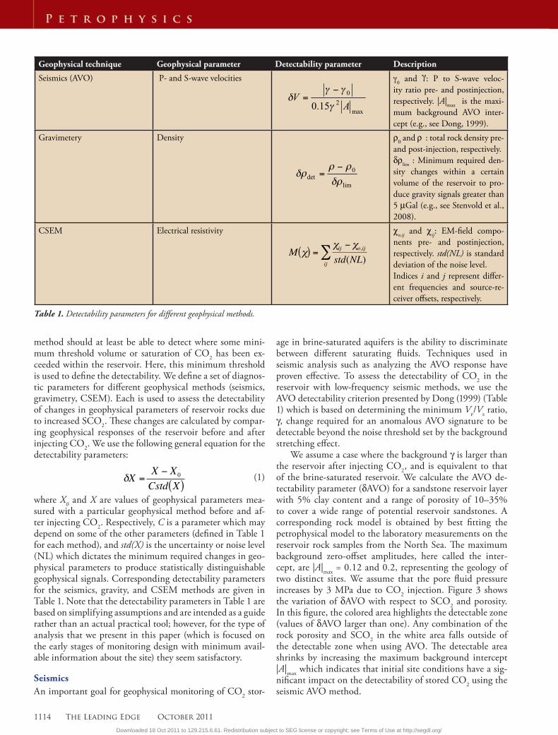
We assume a case where the background γ is larger than the reservoir after injecting CO2, and is equivalent to that of the brine-saturated reservoir. We calculate the AVO de-tectability parameter (δAVO) for a sandstone reservoir layer with 5% clay content and a range of porosity of 10–35% to cover a wide range of potential reservoir sandstones. A corresponding rock model is obtained by best fitting the petrophysical model to the laboratory measurements on the reservoir rock samples from the North Sea. The maximum background zero-offset amplitudes, here called the inter-cept, are |A|max = 0.12 and 0.2, representing the geology of two distinct sites. We assume that the pore fluid pressure increases by 3 MPa due to CO2 injection. Figure 3 shows the variation of δAVO with respect to SCO2 and porosity. In this figure, the colored area highlights the detectable zone (values of δAVO larger than one). Any combination of the rock porosity and SCO2 in the white area falls outside of the detectable zone when using AVO. The detectable area shrinks by increasing the maximum background intercept |A|max which indicates that initial site conditions have a sig-nificant impact on the detectability of stored CO2 using the seismic AVO method.

Geophysical technique Geophysical parameter Detectability parameter Description

Seismics (AVO) P- and S-wave velocities0 and : P to S-wave veloc-

ity ratio pre- and postinjection, respectively. |A|max is the maxi-mum background AVO inter-cept (e.g., see Dong, 1999).

Gravimetery Density ρ0 and ρ : total rock density pre- and post-injection, respectively.δρlim : Minimum required den-sity changes within a certain volume of the reservoir to pro-duce gravity signals greater than 5 μGal (e.g., see Stenvold et al., 2008).

CSEM Electrical resistivity χo,ij and χij: EM-field compo-nents pre- and postinjection, respectively. std(NL) is standard deviation of the noise level.Indices i and j represent differ-ent frequencies and source-re-ceiver offsets, respectively.

Table 1. Detectability parameters for different geophysical methods.




GravimetryOnce CO2 is injected into the brine-saturated rocks (saline aquifer reservoir), it will partially replace the brine and con-sequently change the bulk density of the reservoir rocks. Dif-ferent studies have shown that it is possible to detect the pres-ence of CO2 in the storage formation by gravimetry which is sensitive to these density changes (e.g., Alnes et al., 2008). However, the depth of the storage formation and inherent resolution of the technique have a significant impact on the feasibility of gravimetric detection of CO2 migration. As the depth of the storage formation increases, the amplitude of gravity measurements at the surface decreases rapidly.

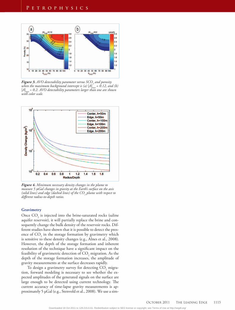
To design a gravimetry survey for detecting CO2 migra-tion, forward modeling is necessary to see whether the ex-pected amplitudes of the generated signals on the surface are large enough to be detected using current technology. The current accuracy of time-lapse gravity measurements is ap-proximately 5 μGal (e.g., Stenvold et al., 2008). We use a sim-

Figure 3. AVO detectability parameter versus SCO2 and porosity when the maximum background intercept is (a) |A|max = 0.12, and (b) |A|max = 0.2. AVO detectability parameters larger than one are shown with color scale.

Figure 4. Minimum necessary density changes in the plume to measure 5 Gal changes in gravity at the Earth’s surface on the axis (solid lines) and edge (dashed lines) of the CO2 plume with respect to different radius-to-depth ratios.




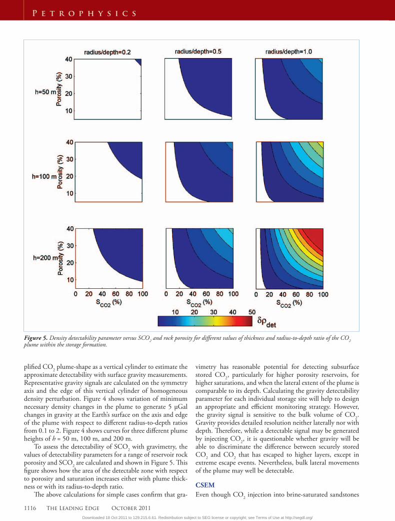
plified CO2 plume-shape as a vertical cylinder to estimate the approximate detectability with surface gravity measurements. Representative gravity signals are calculated on the symmetry axis and the edge of this vertical cylinder of homogeneous density perturbation. Figure 4 shows variation of minimum necessary density changes in the plume to generate 5 μGal changes in gravity at the Earth’s surface on the axis and edge of the plume with respect to different radius-to-depth ratios from 0.1 to 2. Figure 4 shows curves for three different plume heights of h = 50 m, 100 m, and 200 m.

To assess the detectability of SCO2 with gravimetry, the values of detectability parameters for a range of reservoir rock porosity and SCO2 are calculated and shown in Figure 5. This figure shows how the area of the detectable zone with respect to porosity and saturation increases either with plume thick-ness or with its radius-to-depth ratio.

The above calculations for simple cases confirm that gra-

vimetry has reasonable potential for detecting subsurface stored CO2, particularly for higher porosity reservoirs, for higher saturations, and when the lateral extent of the plume is comparable to its depth. Calculating the gravity detectability parameter for each individual storage site will help to design an appropriate and efficient monitoring strategy. However, the gravity signal is sensitive to the bulk volume of CO2. Gravity provides detailed resolution neither laterally nor with depth. Therefore, while a detectable signal may be generated by injecting CO2, it is questionable whether gravity will be able to discriminate the difference between securely stored CO2 and CO2 that has escaped to higher layers, except in extreme escape events. Nevertheless, bulk lateral movements of the plume may well be detectable.

CSEMEven though CO2 injection into brine-saturated sandstones

Figure 5. Density detectability parameter versus SCO2 and rock porosity for different values of thickness and radius-to-depth ratio of the CO2 plume within the storage formation.




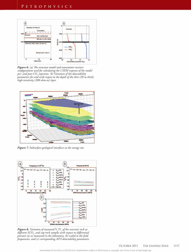
Figure 7. Subsurface geological interfaces at the storage site.

Figure 6. (a) The structure model and transmitter-receiver configurations used for calculating the CSEM response of the model pre- and post-CO2 injection. (b) Variation of the detectability parameters for and with respect to the depth of the thin (20 m thick) high-resistivity (200 ohm-m) layer.

Figure 8. Variation of measured Vp/Vs of the reservoir rock at different SCO2, and cap-rock samples with respect to differential pressure (a) as measured in the laboratory, (b) scaled to the field frequencies, and (c) corresponding AVO detectability parameters.




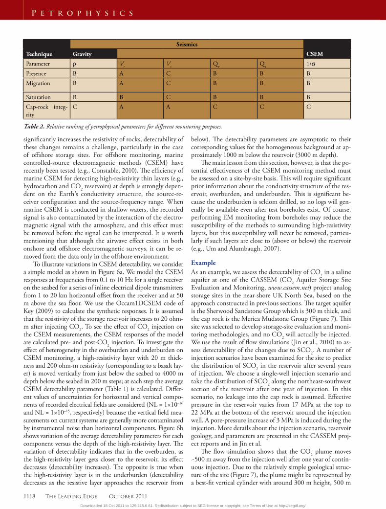
Seismics

Technique Gravity CSEM

Parameter ρ VP

VS

Qp Qs 1/σPresence B A C B B BMigration B A C B B B

Saturation B B C B B BCap-rock integ-rity

C A A C C C

Table 2. Relative ranking of petrophysical parameters for different monitoring purposes.

significantly increases the resistivity of rocks, detectability of these changes remains a challenge, particularly in the case of offshore storage sites. For offshore monitoring, marine controlled-source electromagnetic methods (CSEM) have recently been tested (e.g., Constable, 2010). The efficiency of marine CSEM for detecting high-resistivity thin layers (e.g., hydrocarbon and CO2 reservoirs) at depth is strongly depen-dent on the Earth’s conductivity structure, the source-re-ceiver configuration and the source-frequency range. When marine CSEM is conducted in shallow waters, the recorded signal is also contaminated by the interaction of the electro-magnetic signal with the atmosphere, and this effect must be removed before the signal can be interpreted. It is worth mentioning that although the airwave effect exists in both onshore and offshore electromagnetic surveys, it can be re-moved from the data only in the offshore environment.

To illustrate variations in CSEM detectability, we consider a simple model as shown in Figure 6a. We model the CSEM responses at frequencies from 0.1 to 10 Hz for a single receiver on the seabed for a series of inline electrical dipole transmitters from 1 to 20 km horizontal offset from the receiver and at 50 m above the sea floor. We use the Occam1DCSEM code of Key (2009) to calculate the synthetic responses. It is assumed that the resistivity of the storage reservoir increases to 20 ohm-m after injecting CO2. To see the effect of CO2 injection on the CSEM measurements, the CSEM responses of the model are calculated pre- and post-CO2 injection. To investigate the effect of heterogeneity in the overburden and underburden on CSEM monitoring, a high-resistivity layer with 20 m thick-ness and 200 ohm-m resistivity (corresponding to a basalt lay-er) is moved vertically from just below the seabed to 4000 m depth below the seabed in 200 m steps; at each step the average CSEM detectability parameter (Table 1) is calculated. Differ-ent values of uncertainties for horizontal and vertical compo-nents of recorded electrical fields are considered (NL = 1×10–16 and NL = 1×10–15, respectively) because the vertical field mea-surements on current systems are generally more contaminated by instrumental noise than horizontal components. Figure 6b shows variation of the average detectability parameters for each component versus the depth of the high-resistivity layer. The variation of detectability indicates that in the overburden, as the high-resistivity layer gets closer to the reservoir, its effect decreases (detectability increases). The opposite is true when the high-resistivity layer is in the underburden (detectability decreases as the resistive layer approaches the reservoir from

below). The detectability parameters are asymptotic to their corresponding values for the homogeneous background at ap-proximately 1000 m below the reservoir (3000 m depth).

The main lesson from this section, however, is that the po-tential effectiveness of the CSEM monitoring method must be assessed on a site-by-site basis. This will require significant prior information about the conductivity structure of the res-ervoir, overburden, and underburden. This is significant be-cause the underburden is seldom drilled, so no logs will gen-erally be available even after test boreholes exist. Of course, performing EM monitoring from boreholes may reduce the susceptibility of the methods to surrounding high-resistivity layers, but this susceptibility will never be removed, particu-larly if such layers are close to (above or below) the reservoir (e.g., Um and Alumbaugh, 2007).

ExampleAs an example, we assess the detectability of CO2 in a saline aquifer at one of the CASSEM (CO2 Aquifer Storage Site Evaluation and Monitoring, www.cassem.net) project analog storage sites in the near-shore UK North Sea, based on the approach constructed in previous sections. The target aquifer is the Sherwood Sandstone Group which is 300 m thick, and the cap rock is the Merica Mudstone Group (Figure 7). This site was selected to develop storage-site evaluation and moni-toring methodologies, and no CO2 will actually be injected. We use the result of flow simulations (Jin et al., 2010) to as-sess detectability of the changes due to SCO2. A number of injection scenarios have been examined for the site to predict the distribution of SCO2 in the reservoir after several years of injection. We choose a single-well injection scenario and take the distribution of SCO2 along the northeast-southwest section of the reservoir after one year of injection. In this scenario, no leakage into the cap rock is assumed. Effective pressure in the reservoir varies from 17 MPa at the top to 22 MPa at the bottom of the reservoir around the injection well. A pore-pressure increase of 3 MPa is induced during the injection. More details about the injection scenario, reservoir geology, and parameters are presented in the CASSEM proj-ect reports and in Jin et al.

The flow simulation shows that the CO2 plume moves ~500 m away from the injection well after one year of contin-uous injection. Due to the relatively simple geological struc-ture of the site (Figure 7), the plume might be represented by a best-fit vertical cylinder with around 300 m height, 500 m




radius, and average SCO2 = 30%. The P- and S-wave veloci-ties of the reservoir rock samples taken from a drilled borehole in the region were measured in the laboratory under several differential pressures and saturations (Figure 8). For the cap-rock samples, the measurements were conducted under dry conditions, and we corrected them for the full brine-saturated situation using Gassmann's relation (e.g., Smith et al., 2003) (more details about these measurements are given in CAS-SEM project reports). Because the frequency of the measure-ments in the laboratory (1 MHz) is much higher than the applied frequency in the field (30 Hz), we scale the measured values to the field frequency using the combined petrophysi-cal model (Figure 8b). The Vp/Vs of the reservoir rock and cap rock decreases with different rates with increasing differential pressure. The Vp/Vs of the cap rock is greater than the Vp/Vs of the brine-saturated reservoir rock. Because injection of CO2 into the reservoir leads to the Vp/Vs decrease, then the AVO detectability increases with increasing SCO2 and differential pressure (Figure 8c).

Due to the shallow depth and large thickness of the reser-voir, the gravity method has the potential to monitor the bulk lateral migration of the CO2 plume. The values of the gravity detectability parameters at the axis and edge of the plume are 2.3 and 1.9, respectively. Calculation of the gravity response away from the plume shows that the expected gravity change is below the instrumental noise at 1350 m from the axis of the plume (850 m from the plume edge). Knowing this distance is valuable for designing the gravity-monitoring grid.

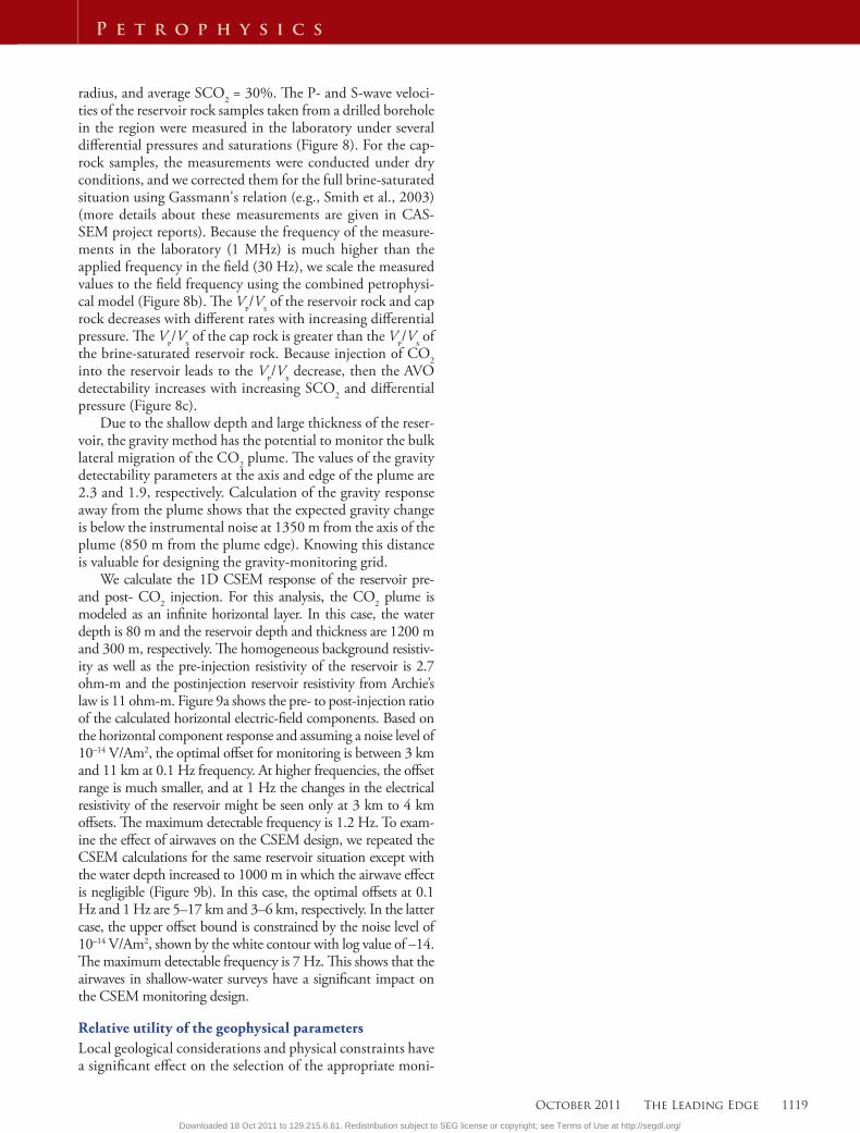
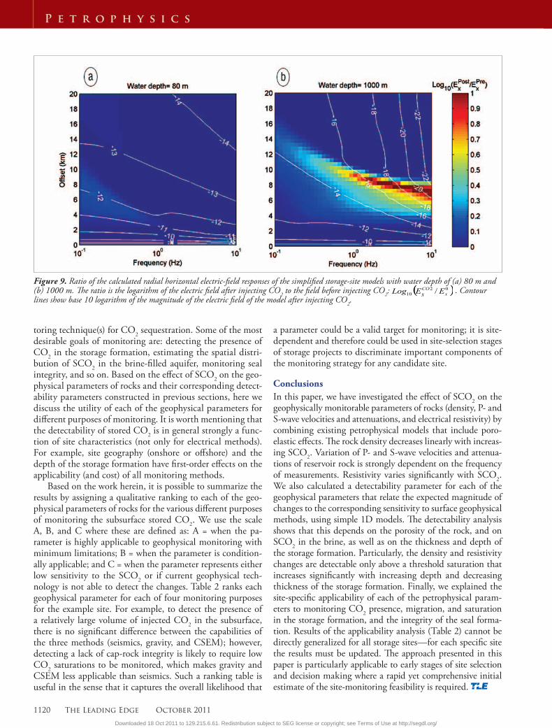
We calculate the 1D CSEM response of the reservoir pre- and post- CO2 injection. For this analysis, the CO2 plume is modeled as an infinite horizontal layer. In this case, the water depth is 80 m and the reservoir depth and thickness are 1200 m and 300 m, respectively. The homogeneous background resistiv-ity as well as the pre-injection resistivity of the reservoir is 2.7 ohm-m and the postinjection reservoir resistivity from Archie’s law is 11 ohm-m. Figure 9a shows the pre- to post-injection ratio of the calculated horizontal electric-field components. Based on the horizontal component response and assuming a noise level of 10–14 V/Am2, the optimal offset for monitoring is between 3 km and 11 km at 0.1 Hz frequency. At higher frequencies, the offset range is much smaller, and at 1 Hz the changes in the electrical resistivity of the reservoir might be seen only at 3 km to 4 km offsets. The maximum detectable frequency is 1.2 Hz. To exam-ine the effect of airwaves on the CSEM design, we repeated the CSEM calculations for the same reservoir situation except with the water depth increased to 1000 m in which the airwave effect is negligible (Figure 9b). In this case, the optimal offsets at 0.1 Hz and 1 Hz are 5–17 km and 3–6 km, respectively. In the latter case, the upper offset bound is constrained by the noise level of 10–14 V/Am2, shown by the white contour with log value of –14. The maximum detectable frequency is 7 Hz. This shows that the airwaves in shallow-water surveys have a significant impact on the CSEM monitoring design.

Relative utility of the geophysical parametersLocal geological considerations and physical constraints have a significant effect on the selection of the appropriate moni-




Figure 9. Ratio of the calculated radial horizontal electric-field responses of the simplified storage-site models with water depth of (a) 80 m and (b) 1000 m. The ratio is the logarithm of the electric field after injecting CO2 to the field before injecting CO2: . Contour lines show base 10 logarithm of the magnitude of the electric field of the model after injecting CO2.

toring technique(s) for CO2 sequestration. Some of the most desirable goals of monitoring are: detecting the presence of CO2 in the storage formation, estimating the spatial distri-bution of SCO2 in the brine-filled aquifer, monitoring seal integrity, and so on. Based on the effect of SCO2 on the geo-physical parameters of rocks and their corresponding detect-ability parameters constructed in previous sections, here we discuss the utility of each of the geophysical parameters for different purposes of monitoring. It is worth mentioning that the detectability of stored CO2 is in general strongly a func-tion of site characteristics (not only for electrical methods). For example, site geography (onshore or offshore) and the depth of the storage formation have first-order effects on the applicability (and cost) of all monitoring methods.

Based on the work herein, it is possible to summarize the results by assigning a qualitative ranking to each of the geo-physical parameters of rocks for the various different purposes of monitoring the subsurface stored CO2. We use the scale A, B, and C where these are defined as: A = when the pa-rameter is highly applicable to geophysical monitoring with minimum limitations; B = when the parameter is condition-ally applicable; and C = when the parameter represents either low sensitivity to the SCO2 or if current geophysical tech-nology is not able to detect the changes. Table 2 ranks each geophysical parameter for each of four monitoring purposes for the example site. For example, to detect the presence of a relatively large volume of injected CO2 in the subsurface, there is no significant difference between the capabilities of the three methods (seismics, gravity, and CSEM); however, detecting a lack of cap-rock integrity is likely to require low CO2 saturations to be monitored, which makes gravity and CSEM less applicable than seismics. Such a ranking table is useful in the sense that it captures the overall likelihood that

a parameter could be a valid target for monitoring; it is site-dependent and therefore could be used in site-selection stages of storage projects to discriminate important components of the monitoring strategy for any candidate site.

ConclusionsIn this paper, we have investigated the effect of SCO2 on the geophysically monitorable parameters of rocks (density, P- and S-wave velocities and attenuations, and electrical resistivity) by combining existing petrophysical models that include poro-elastic effects. The rock density decreases linearly with increas-ing SCO2. Variation of P- and S-wave velocities and attenua-tions of reservoir rock is strongly dependent on the frequency of measurements. Resistivity varies significantly with SCO2. We also calculated a detectability parameter for each of the geophysical parameters that relate the expected magnitude of changes to the corresponding sensitivity to surface geophysical methods, using simple 1D models. The detectability analysis shows that this depends on the porosity of the rock, and on SCO2 in the brine, as well as on the thickness and depth of the storage formation. Particularly, the density and resistivity changes are detectable only above a threshold saturation that increases significantly with increasing depth and decreasing thickness of the storage formation. Finally, we explained the site-specific applicability of each of the petrophysical param-eters to monitoring CO2 presence, migration, and saturation in the storage formation, and the integrity of the seal forma-tion. Results of the applicability analysis (Table 2) cannot be directly generalized for all storage sites—for each specific site the results must be updated. The approach presented in this paper is particularly applicable to early stages of site selection and decision making where a rapid yet comprehensive initial estimate of the site-monitoring feasibility is required.




ReferencesAlnes, H., O. Eiken, and T. Stenvold, 2008, Monitoring gas production

and CO2 injection at the Sleipner field using time-lapse gravimetry: Geophysics, 73, no. 6, WA155–WA161, doi:10.1190/1.2991119.

Archie, G. E., 1942, The electrical resistivity log as an aid in determin-ing some reservoir characteristics: Transactions of the American Institute of Mining, Metallurgical and Petroleum Engineers, 146, 54–62.

Constable, S., 2010, Ten years of marine CSEM for hydrocarbon ex-ploration; Geophysics, 75, no. 5, 75A67–75A81.

Dong, W., 1999, AVO detectability against tuning and stretching ar-tefacts: Geophysics, 64, no. 2, 494–503, doi:10.1190/1.1444555.

Jin, M., J. Pickup, E. Mackay, A. Todd, A. Monaghan, and M. Naylor, 2010, Static and dynamic estimates of CO2 storage capacity in two saline formations in the UK: SPE paper 131609.

Key, K., 2009, 1D inversion of multicomponent, multifrequency ma-rine CSEM data: Methodology and synthetic studies for resolving thin resistive layers: Geophysics, 74, F9, doi:10.1190/1.3058434.

Mavko, G., T. Mukerji, and J. Dvorkin, 1998, Rock physics hand-book: Cambridge University Press.

Pham, N. H., J. M. Carcione, H. B. Helle, and B. Ursin, 2002, Wave velocities and attenuation of shaley sandstones as a function of pore pressure and partial saturation: Geophysical Prospecting, 50, no. 6, 615–627, doi:10.1046/j.1365-2478.2002.00343.x.

Pride, S. R., J. G. Berryman, and J. M. Harris, 2004, Seismic attenu-ation due to wave-induced flow: Journal of Geophysical Research, 109, B1, B01201, doi:10.1029/2003JB002639.

Smith, T. M., C. H. Sondergeld, and C. S. Rai, 2003, Gassmann fluid substitutions: A tutorial: Geophysics, 68, no. 2, 430–440, doi:10.1190/1.1567211.

Stenvold, T., O. Eiken, and M. Landrø, 2008, Gravimetric monitor-ing of gas-reservoir water influx—A combined flow- and grav-ity-modeling approach: Geophysics, 73, no. 6, WA123–WA131, doi:10.1190/1.2991104.

Um, E. S. and D. L. Alumbaugh, 2007, On the physics of the marine controlled-source electromagnetic method: Geophysics, 72, no. 2, WA13–WA26, doi:10.1190/1.2432482.

White, J. E., 1975, Computed seismic speeds and attenuation in rocks with partial gas saturation: Geophysics, 40, no. 2, 224–232, doi:10.1190/1.1440520.

Acknowledgments: The research related to this paper has been carried out within the CASSEM project, a project supported by the Technology Strategy Board (TSB). The authors acknowledge the support of the TSB and the EPSRC and the project industry partners AMEC, Marathon, Schlumberger, Scottish Power, and Scottish and Southern Energy; and the academic partners, The British Geological Survey, Heriot-Watt University, University of Edinburgh, and the University of Manchester. We also thank Quentin Fisher and his colleagues at the University of Leeds for providing us with the laboratory measurements.

Corresponding author: [email protected]

Editor's note: Arash JafarGandomi is now with the Lancaster Envi-ronment Centre, Lancaster University.


Documents

saturated aquifer reservoirs using surface geophysical methods