Embed Size (px)
Citation preview
Felix BoyIn the design of modern electrical drives a trend towards higher speeds and lighter structures can be observed. While increasing the power density this trend also implies stronger vibration issues. Among these phenomena lateral rotor oscillations due to unbalanced magnetic pull are of particular interest: strong lateral vibrations may lead to rotor-stator contact destroying the system in extreme cases.
In this work an electromechanical model is established to describe such rotordynamic vibrations. It is applicable to all kinds of rotating field machines and captures arbitrary transient states. The model describes both currents and rotor motion in a fully coupled manner. It accounts for higher harmonics in the air-gap flux density, magnetic saturation and parallel branches in the winding. The model is vali-dated by comparing it to finite element simulations, measurements and space vector models. The examples chosen are a cage induction machine and an permanent magnet synchronous machine.
Using the model self-excited rotor oscillations have been investiga-ted. Based on several simulation studies simple formulae for critical speeds concerning these vibrations have been established.
9 783737 609166
ISBN 978-3-7376-0916-6
Modelling the Rotordynamics of Saturated Electrical Machines
due to Unbalanced Magnetic Pull
Felix Boy
Modelling the Rotordynamics of Saturated Electrical Machines due to Unbalanced Magnetic Pull
This work has been accepted by Faculty of Mechanical Engineering of the University of Kassel as a thesis for acquiring the academic degree of Doktor der Ingenieurwissenschaften (Dr.-Ing.).
Supervisor: Univ. Prof. Dr.-Ing. Hartmut Hetzler, University of Kassel Co-Supervisor: Univ. Prof. Dr.-Ing. Jana Kertzscher, TU Bergakademie Freiberg Defense day: 17. July 2020
This document – excluding quotations and otherwise identified parts – is licensed under the Creative Commons Attribution-Share Alike 4.0 International License (CC BY-SA 4.0: https://creativecommons.org/licenses/by-sa/4.0/)
https://orcid.org/0000-0002-0063-9475 (Felix Boy)
Bibliographic information published by Deutsche Nationalbibliothek The Deutsche Nationalbibliothek lists this publication in the Deutsche Nationalbibliografie; detailed bibliographic data is available in the Internet at http://dnb.dnb.de.
Zugl.: Kassel, Univ., Diss. 2020 ISBN 978-3-7376-0916-6 DOI: https://dx.doi.org/doi:10.17170/kobra-202010272016
© 2020, kassel university press, Kassel http://kup.uni-kassel.de
Printed in Germany
Preface
The work described in this thesis has been conducted at the Engineering
Dynamics Group at the University of Kassel from 2014 to 2019.
I would like to express my deep gratitude to my supervisor Professor Hart-
mut Hetzler for his invaluable support and guidance through five years of
interesting discussions and many long hours of work. I could not be more
thankful for his trust and patience even in stressful situations and the
fact, that he always had time for discussions if needed. His unbreakable
enthusiasm both in teaching and research has always been an inspiring
example to me.
It is impossible to overestimate the help and motivation I experienced by
having such good friends and colleagues in our group. Besides giving me
good advice, or discussing in depth problems, I mostly appreciate their
unparalleled ability and will to create a both fruitful and focussed wor-
king atmosphere.
I am very thankful to Professor Jana Kertzscher for taking on the task
of co-supervising this thesis. Moreover, I would like to express my heart-
ful gratitude to her and Johannes Paul Vogt for sharing their profound
knowledge with me and providing me their data and information on the
E-FFEKT cage induction machine. Learning from them at the TU Berg-
akademie in Freiberg has been a great pleasure.
V

I would like to thank Dr. Timo Holopainen, Dr. Ulrich Romer and Pro-
fessor Jorg Wauer for very interesting and helpful discussions and their
thoughtful advice on the thesis. Furthermore, I am most thankful to Kyle
Kenney for his support on language matters.
The support, help and assistance in terms of encouragement, motivation
and happiness my family gave me made it possible for me to conduct this
work and I would like to express my deep and heartful thankfulness to
them.
Kassel, August 2019
Felix Benjamin Boy
VI
AbstractIn the design of modern electrical drives a trend towards higher speeds
and lighter structures can be observed. While increasing the power density
this trend also implies stronger vibration issues. Among these phenomena
lateral rotor oscillations due to unbalanced magnetic pull are of particular
interest: when running at high speeds, strong lateral vibrations may lead
to rotor-stator contact destroying the system in extreme cases.
In this work an electromechanical model is established to describe and
assess such rotordynamic vibrations. It is applicable to all kinds of ra-
dial flux rotating field machines and captures arbitrary transient states.
The model describes both currents and rotor motion in a fully coupled
manner. It accounts for higher harmonics in the air-gap flux density, ma-
gnetic saturation and parallel branches in the winding. The model is two
dimensional, i.e. effects of homopolar fluxes, or rotor skew are neglected.
The proposed approach is based on a semi-analytical solution of the ma-
gnetic field problem. This new method combines magnetic equivalent cir-
cuits and an analytical solution of the air-gap field providing the advanta-
ge of high computational efficiency while considering non-linear magnetic
effects. The model is validated by comparing it to finite element simulati-
ons, measurements and space vector models. The examples chosen are a
cage induction machine and an interior permanent magnet synchronous
machine.
Using the derived model self-excited rotor oscillations due to induction in
the rotor cage and into parallel branches of the stator winding have been
investigated. Extending earlier findings and based on several simulation
studies, simple formulae for critical speeds concerning these vibrations
have been established.
VII

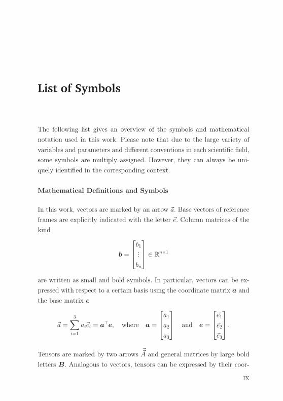
List of Symbols
The following list gives an overview of the symbols and mathematical
notation used in this work. Please note that due to the large variety of
variables and parameters and different conventions in each scientific field,
some symbols are multiply assigned. However, they can always be uni-
quely identified in the corresponding context.
Mathematical Definitions and Symbols
In this work, vectors are marked by an arrow �a. Base vectors of reference
frames are explicitly indicated with the letter �e. Column matrices of the
kind
b =
⎡⎢⎣b1...bn
⎤⎥⎦ ∈ R
n×1
are written as small and bold symbols. In particular, vectors can be ex-
pressed with respect to a certain basis using the coordinate matrix a and
the base matrix e
�a =3∑i=1
ai�ei = a�e, where a =
⎡⎢⎣a1a2a3
⎤⎥⎦ and e =
⎡⎢⎣�e1�e2�e3
⎤⎥⎦ .
Tensors are marked by two arrows��A and general matrices by large bold
letters B. Analogous to vectors, tensors can be expressed by their coor-
IX
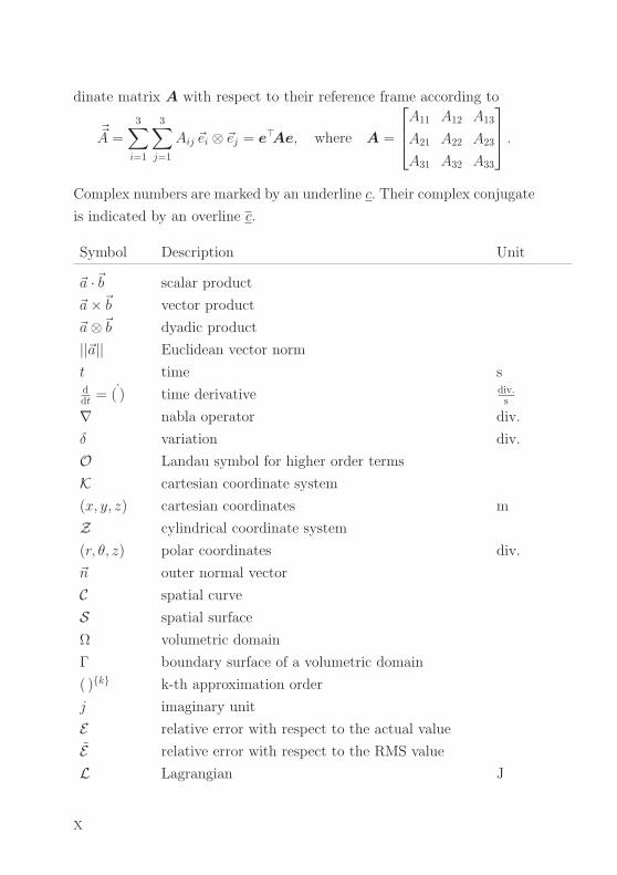
dinate matrix A with respect to their reference frame according to
��A =3∑i=1
3∑j=1
Aij �ei ⊗ �ej = e�Ae, where A =
⎡⎢⎣A11 A12 A13
A21 A22 A23
A31 A32 A33
⎤⎥⎦ .
Complex numbers are marked by an underline c. Their complex conjugate
is indicated by an overline c.
Symbol Description Unit
�a ·�b scalar product
�a�b vector product
�a⊗�b dyadic product
||�a|| Euclidean vector norm
t time sddt =
˙( ) time derivative div.s
∇ nabla operator div.
δ variation div.
O Landau symbol for higher order terms
K cartesian coordinate system
(x, y, z) cartesian coordinates m
Z cylindrical coordinate system
(r, θ, z) polar coordinates div.
�n outer normal vector
C spatial curve
S spatial surface
Ω volumetric domain
Γ boundary surface of a volumetric domain
( ){k} k-th approximation order
j imaginary unit
E relative error with respect to the actual value
E relative error with respect to the RMS value
L Lagrangian J
X
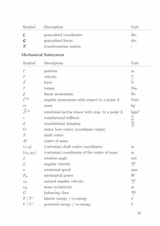
Symbol Description Unit
ξ generalised coordinates div.
G generalised forces div.
T transformation matrix -
Mechanical Subsystem
Symbol Description Unit
�r position m
�v velocity ms
�f force N
�τ torque Nm
�p linear momentum Ns�� (A) angular momentum with respect to a point A Nms
m mass kg��J (A) rotational inertia tensor with resp. to a point A kgm2
c translational stiffness Nm
d translational damping Nsm
O stator bore centre (coordinate origin)
S shaft centre
M centre of mass
(x, y) (cartesian) shaft centre coordinates m
(xG, yG) (cartesian) coordinates of the centre of mass m
φ rotation angle rad
�ω angular velocity rads
n rotational speed rpm
Pm mechanical power W
ω0 natural angular velocity rads
eM mass eccentricity m
G balancing class mms
T / T ∗ kinetic energy / co-energy J
V / V ∗ potential energy / co-energy J
XI
Electrical Subsystem
Symbol Description Unit
�e electric field Vm
�d electric displacement field Asm2
�j current density Am2
�p electric polarization Asm2
ε0 electric field constant Fm
ϕ electric potential V
q charge C
i current A
v voltage V��S electrical conductivity tensor A
Vm
Re electrical resistance Ω
C electrical capacitance F
Pe electrical power W
We /W∗e electric energy / co-energy J
i generalised currents A
v generalised voltage V
Magnetic Field Problem
Symbol Description Unit
�b magnetic flux density T�h magnetic field A
m
�m magnetisation Am
��Tmag Maxwell stress tensor Nm2
F magnetic scalar potential A
�a magnetic vector potential Tm
μ0 magnetic constant TmA
Φ magnetic flux Wb
XII
Symbol Description Unit
λ magnetic flux linkage Wb
L inductance H
R1 stator bore radius m
R2 rotor radius m
R average air-gap radius m
� axial machine length (effective) m
δ0 nominal air-gap width (centred rotor) m
δ air-gap width (arbitrary rotor position) m
R2δ parametrised rotor surface (eccentric rotor) m
Λ air-gap permeance TA
f boundary magneto-motive force A
ε small parameter
e eccentricity m
ρ specific eccentricity
γ eccentricity phase angle rad
e0 static eccentricity m
γ0 static eccentricity phase angle rad
ed dynamic eccentricity m
γd dynamic eccentricity phase angle rad
Wmag /W∗mag magnetic energy / co-energy J
XIII
Contents
Preface V
Abstract VII
List of Symbols IX
1 Introduction 1
1.1 State of the Art 7
1.1.1 Calculation of the Magnetic Field and Forces 7
1.1.2 Dynamics due to Magnetic Interactions 17
1.2 Aims and Structure of the Work 25
2 Model 28
2.1 Problem Formulation and Overview 28
2.1.1 Governing Equations 29
2.1.2 Fundamental Assumptions and their Implications 36
2.2 Electromechanical System Equations 45
2.2.1 The Classical Approach (Newton-Faraday) 45
2.2.2 The Analytical Approach (Lagrange-Maxwell) 47
2.2.3 Comparing the Classical and Analytical Approaches 51
2.2.4 Qualitative Behaviour of the Coupling 54
2.2.5 Conclusions 56
2.3 Mechanical Subsystem 57
2.3.1 Misalignments (Eccentricities) 61
2.3.2 Kinematics 64
2.3.3 Kinetics 67
2.3.4 Conclusions 70
2.4 Electrical Subsystem 71
2.4.1 Generalised currents 74
2.4.2 Generalised mesh equations 76
2.4.3 Equivalence of Generalised Mesh and Nodal Analysis 83
2.4.4 Phase Connections 85
2.4.5 Conclusions 87
2.5 Magnetic Field Problem 88
2.5.1 Air-Gap Domain (Asymptotic Expansion) 93
2.5.2 Solid Domains (AN-MEC Approach) 109
2.5.3 Conclusions 117
2.6 Electromechanical Coupling 118
2.6.1 The Classical Coupling (Newton-Faraday) 118
2.6.2 The Analytical Coupling (Lagrange-Maxwell) 119
2.6.3 Equivalence of the Classical and Analytical Coupling 121
2.6.4 Conclusions 128
2.7 Complete System of Differential Equations 129
2.7.1 Resulting Equations 129
2.7.2 Numerical Implementation 131
2.7.3 Computational Efficiency 133
3 Validation 137
3.1 Cage Induction Machine 141
3.1.1 Static Validation (FEM) 141
3.1.2 Dynamic Validation (Space Vector) 148
3.2 Interior Permanent Magnet Synchronous Machine 152
3.2.1 Static Validation (FEM) 153
3.2.2 Dynamic Validation (Space Vector) 161
3.3 Conclusions 167
4 Results 168
4.1 Cage Induction Machine 169
4.1.1 Simulation Studies 172
4.1.2 Generalisation: Physical Cause and Practical Assess-
ment of Self-Excited Rotor Oscillations due to the Ro-
tor Cage 182
4.1.3 Modelling Aspects and Parameter Studies 190
4.2 Interior Permanent Magnet Synchronous Machine 196
4.2.1 Simulation Studies 197
4.2.2 Generalisation: Physical Cause and Practical Assess-
ment of Self-Excited Rotor Oscillations due to Parallel
Branches 207
4.3 Conclusions 209
5 Conclusions and Suggestions for Further Work 212
References 220
Publications during the Doctorate 237
A Fundamentals on Electromechanical Energy Functionals 239
B Asymptotic Expansion of the Air-Gap Magnetic Field 249
C Basic Equations for Magnetic Equivalent Circuits 257
D Machines and Models 262

1 Introduction
In the past decades fields of application for rotating field electrical machi-
nes have changed significantly [1, p. XXI]. Starting with the development
of modern power electronics, variable speed drives have become the stan-
dard in industry and on the consumer marked. A comparably new trend
has been started with the increasing interest in electric vehicles [2, p. 4]:
compared to earlier applications (as for example in trains), such applica-
tions require advanced lightweight design and a high power density, while
maintaining the reliability necessary for a save operation.
One of the most effective ways to achieve a higher power density is in-
creasing the machine speed. In fact, a trend towards higher speeds in
electric vehicle drives can be directly observed [3, p. 3]. One of the most
illustrating examples is the Toyota Prius traction drive. While in 2006 it
was designed for a maximum speed of 6000 rpm, the next generations in
2010 and 2016 already reached up to 13500 and 17000 rpm respectively
[4]. Apparently, advanced applications propell this trend even further as
for example cutting edge Formula E motors already run at up to 20000
rpm [5].
However, this increased power density comes at a cost: lighter systems
running at higher speeds tend to increase vibration problems [3, p. 8].
Such issues may be of concern, when considering the noise and vibration
harshness (NVH), the machine reliability (in terms of lifetime), or even
the system security (in case of catastrophic failure).
1
1 Introduction
From a scientific point of view it is interesting to note that while the
trend towards higher speeds has led to an increasing research interest
in the design of such devices, the research on structural vibrations, or
rotordynamics in electric machines lags behind. This is contradictory to
a certain extend as an increase in structural and rotor vibrations are a
direct consequence of higher speeds.
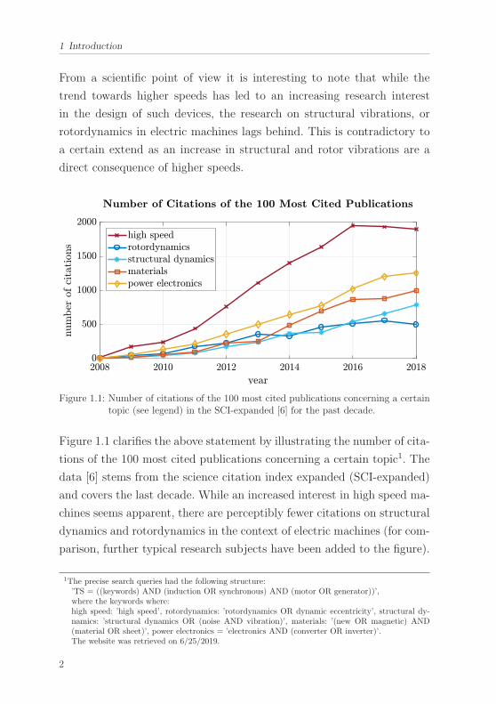
Figure 1.1: Number of citations of the 100 most cited publications concerning a certaintopic (see legend) in the SCI-expanded [6] for the past decade.
Figure 1.1 clarifies the above statement by illustrating the number of cita-
tions of the 100 most cited publications concerning a certain topic1. The
data [6] stems from the science citation index expanded (SCI-expanded)
and covers the last decade. While an increased interest in high speed ma-
chines seems apparent, there are perceptibly fewer citations on structural
dynamics and rotordynamics in the context of electric machines (for com-
parison, further typical research subjects have been added to the figure).
1The precise search queries had the following structure:’TS = ((keywords) AND (induction OR synchronous) AND (motor OR generator))’,where the keywords where:high speed: ’high speed’, rotordynamics: ’rotordynamics OR dynamic eccentricity’, structural dy-namics: ’structural dynamics OR (noise AND vibration)’, materials: ’(new OR magnetic) AND(material OR sheet)’, power electronics = ’electronics AND (converter OR inverter)’.The website was retrieved on 6/25/2019.
2
While intense effort is put into understanding rotor vibrations in other
machine types, as for example turbomachines, drills, or pumps (cf. [7]),
the rotordynamics of electrical machines have not been discussed to a
high degree thus far. This circumstance might be due to two major rea-
sons: first and as mentioned before, the speed of electrical machines has
been comparably low in earlier years. Second, most devices are designed
to have a very stiff bearing arrangement, causing a high critical bending
speed. In fact, still today a large class of electric motors operates below
this threshold (especially smaller machines). However, when considering
the earlier mentioned trend towards higher speeds and lightweight design
this may change in future applications.
Nevertheless, rotor vibrations may become dangerous even in classical
machine designs and lead to a complete system failure, as several cases
from the literature and reports from industry demonstrate. For exam-
ple, Kellenberger [8] reported strong lateral vibrations in a 2-pole turbo
generator. Talas and Toom [9] investigated the rotor-stator contact of a
184 MVA power generator at the Peace Canyon river dam in Canada.
Fruchtenicht et al. [10] investigated strong bending vibrations of a 11 kW
cage induction motor on a test rig. They reported, that similar problems
also arose in a commercial 400 kW motor.
Beyond such published failures, practitioners from industry regularly re-
port on machine break downs which often cannot be clearly assigned to
a specific cause. Typically, these cases are simply explained by ’inap-
propriate operation’ or ’mechanical failure’. A recent example has been
observed in two 112 kW surface mount permanent magnet synchronous
motors, which were used as drives of a test rig in the Institute of Product
Engineering at the Karlsruhe Institute of Technology. Here, the motors
where destroyed shortly one after another, showing similar damage marks
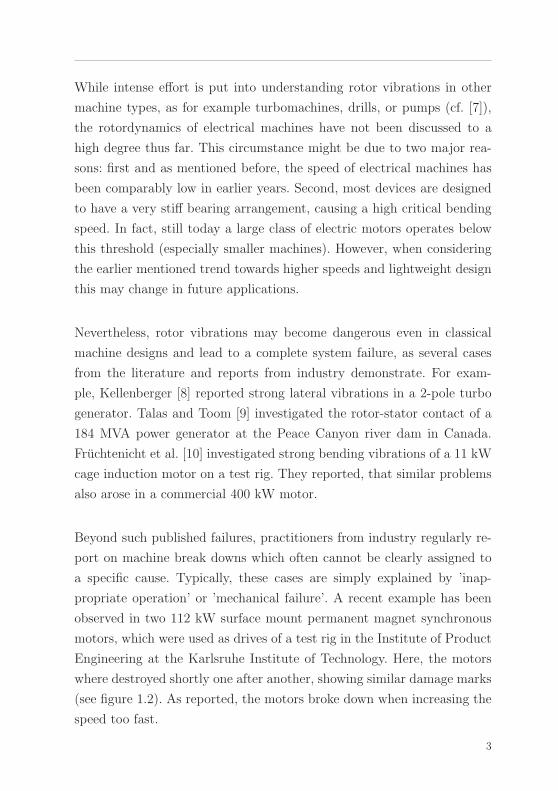
(see figure 1.2). As reported, the motors broke down when increasing the
speed too fast.
3
1 Introduction
When disassembling one of them, it turned out that the bearings where
fully intact, but that the rotor was massively damaged and that there
were grinding marks at the stator. The surface magnets had been pulled
out over large areas and some of the binding bands were ripped apart.
Obviously, the rotor and stator came into contact and some kind of pa-
rasitic forces must have evolved, destroying the system during transient
operation.
a) b) c)
Figure 1.2: Machine failure example from the Institute of Product Engineering at theKarlsruhe Institute of Technology. a) Disassembled motor, b) Detail of thedamages at the rotor, c) Grinding marks at the stator (with backlight for abetter contrast).
A particular challenge in understanding rotor vibrations of electric ma-
chines stems from the fact that they may be caused by an unsymmetric
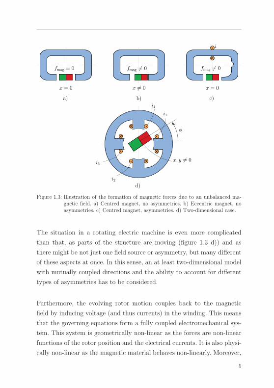
magnetic field [11, p. 10]. To get an intuition for this phenomenon consi-
der a permanent magnet held into an air-gap between two iron surfaces
(figure 1.3 a)). As long as the magnet is centred and as the magnetic field
is distributed symmetrically on both sides of the magnet no resulting
magnetic force will be present. However, the picture changes if motion,
additional field sources (currents/magnets), or some other asymmetries
come into play (figures 1.3 b),c)).
4
a)
x = 0
fmag = 0
x �= 0
b) c)
x = 0
fmag �= 0
i
fmag �= 0
d)
x, y �= 0
φ
i1
i2
i3
i4
Figure 1.3: Illustration of the formation of magnetic forces due to an unbalanced ma-gnetic field. a) Centred magnet, no asymmetries. b) Eccentric magnet, noasymmetries. c) Centred magnet, asymmetries. d) Two-dimensional case.
The situation in a rotating electric machine is even more complicated
than that, as parts of the structure are moving (figure 1.3 d)) and as
there might be not just one field source or asymmetry, but many different
of these aspects at once. In this sense, an at least two-dimensional model
with mutually coupled directions and the ability to account for different
types of asymmetries has to be considered.
Furthermore, the evolving rotor motion couples back to the magnetic
field by inducing voltage (and thus currents) in the winding. This means
that the governing equations form a fully coupled electromechanical sys-
tem. This system is geometrically non-linear as the forces are non-linear
functions of the rotor position and the electrical currents. It is also physi-
cally non-linear as the magnetic material behaves non-linearly. Moreover,
5
1 Introduction
electrical machines and thus their dynamics occur in manifold variations
(think of different machine types, windings, sizes). Taking all these facts
into consideration it seems obvious that their rotordynamics is a complex
research field.
Based on the explanations and case studies above it seems that rotor
oscillations may occur in various machine types and under very different
operational conditions. As the physical reason for the occurrence of the-
se phenomena is rather complicated and non-intuitive, it seems plausible
that in many cases the problem may be either falsely assigned to other
system components (as for example defective bearings etc.), or explained
in an oversimplified manner.
It is therefore the aim of this work to derive a physical model describing
lateral rotor oscillations for various machines and transient operational
states. The model is intended to combine the dynamics of the mechanical
motion and the electrical currents to capture the full electromechanical
coupling in terms of magnetic forces and motional induction. The most
relevant effects like magnetic saturation, or different winding designs (in-
cluding parallel branches) shall be covered.
In order to provide for an overview on already existent approaches, a
literature review concerning the modelling of rotor vibrations will be gi-
ven next. Subsequently, the detailed aims of the present thesis will be
presented and the structure of the work will be outlined.
6
1.1 State of the Art
1.1 State of the Art
Understanding the origin of lateral rotor oscillations due to magnetic ef-fects comprises two fundamental aspects: first, it is necessary to calculatethe magnetic field, the arising forces and induction effects depending onthe electrical currents and the mechanical rotor motion. Second, if thisfunctional relation is known the dynamic consequences of the magneticinteraction have to be analysed. Based on these two points, this literaturereview is subdivided in two parts concerning
1. The calculation of the magnetic field, forces and induction.
2. The analysis of the dynamics due to magnetic interactions.
These topics are embedded into the much larger research field of model-
ling electrical machines in general. As the particular subject discussed in
this review addresses a very small subset of this field, it must be con-
sidered as by no means comprehensive, but focused on the issues men-
tioned above. The types of problems considered in the first part of this
review are restricted to radial flux, rotating field machines and mainly
two-dimensional problems. In the second part, only asynchronous and
synchronous machines are considered. For more comprehensive informa-
tion refer to Chapman [1], Binder [12], or Muller et al. [13].
1.1.1 Calculation of the Magnetic Field and Forces
Approaches to calculate the magnetic field and forces can be roughly
subdivided into analytical models and numerical schemes. Analytical me-
thods bring the advantage of lower computational effort and a better
physical insight. However, numerical approaches are often more accurate
when more detailed models are analysed.
Analytical Methods
Understanding the origin of magnetic forces in electrical machines started
at the beginning of the 20th century with graphically motivated formulae
7
1 Introduction
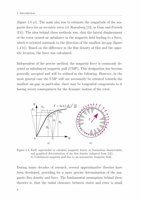
(figure 1.4 a)). The main aim was to estimate the magnitude of the ma-
gnetic force for an eccentric rotor (cf. Rosenberg [14], or Gray and Pertsch
[15]). The idea behind these methods was, that the lateral displacement
of the rotor caused an unbalance in the magnetic field leading to a force,
which is oriented outwards to the direction of the smallest air-gap (figure
1.4 b)). Based on the difference in the flux density at this and the oppo-
site location, the force was calculated.
Independent of the precise method, the magnetic force is commonly de-
noted as unbalanced magnetic pull (UMP). This designation has become
generally accepted and will be utilised in the following. However, in the
most general case the UMP will not necessarily be oriented towards the
smallest air-gap: in particular, there may be tangential components to it
having severe consequences for the dynamic motion of the rotor.
a) b)
0 N
MM1
M2
BB2
B1
H
B
X1
X2F = 2pA
(B
5000
)2 dBdH
F
Figure 1.4: Early approaches to calculate magnetic forces. a) Saturation characteristicand graphical determination of the flux density (adapted from [14]) ,b) Unbalanced magnetic pull due to an asymmetric magnetic field.
During many decades of research, several approximative theories have
been developed, providing for a more precise determination of the ma-
gnetic flux density and force. The fundamental assumption behind these
theories is, that the radial clearance between stator and rotor is small
8
1.1 State of the Art
compared to their diameter. Furthermore, they neglected any influence
of the magnetic field in the solids. Thus, by excluding saturation effects
it became possible to focus the analysis to the machine part where the
electromechanical energy transfer takes place: the air-gap.
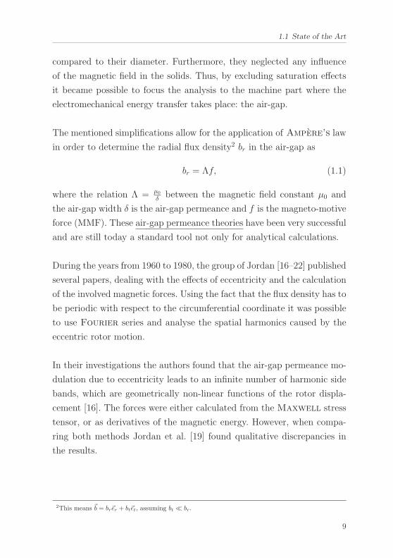
The mentioned simplifications allow for the application of Ampere’s law
in order to determine the radial flux density2 br in the air-gap as
br = Λf, (1.1)
where the relation Λ = μ0
δ between the magnetic field constant μ0 and
the air-gap width δ is the air-gap permeance and f is the magneto-motive
force (MMF). These air-gap permeance theories have been very successful
and are still today a standard tool not only for analytical calculations.
During the years from 1960 to 1980, the group of Jordan [16–22] published
several papers, dealing with the effects of eccentricity and the calculation
of the involved magnetic forces. Using the fact that the flux density has to
be periodic with respect to the circumferential coordinate it was possible
to use Fourier series and analyse the spatial harmonics caused by the
eccentric rotor motion.
In their investigations the authors found that the air-gap permeance mo-
dulation due to eccentricity leads to an infinite number of harmonic side
bands, which are geometrically non-linear functions of the rotor displa-
cement [16]. The forces were either calculated from the Maxwell stress
tensor, or as derivatives of the magnetic energy. However, when compa-
ring both methods Jordan et al. [19] found qualitative discrepancies in
the results.
2This means �b = br�er + bt�et, assuming bt � br.
9
1 Introduction
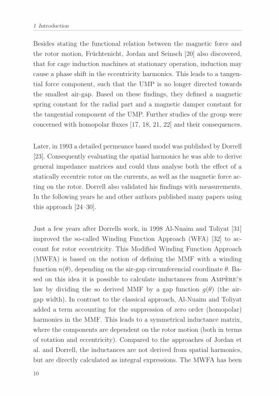
Besides stating the functional relation between the magnetic force and
the rotor motion, Fruchtenicht, Jordan and Seinsch [20] also discovered,
that for cage induction machines at stationary operation, induction may
cause a phase shift in the eccentricity harmonics. This leads to a tangen-
tial force component, such that the UMP is no longer directed towards
the smallest air-gap. Based on these findings, they defined a magnetic
spring constant for the radial part and a magnetic damper constant for
the tangential component of the UMP. Further studies of the group were
concerned with homopolar fluxes [17, 18, 21, 22] and their consequences.
Later, in 1993 a detailed permeance based model was published by Dorrell
[23]. Consequently evaluating the spatial harmonics he was able to derive
general impedance matrices and could thus analyse both the effect of a
statically eccentric rotor on the currents, as well as the magnetic force ac-
ting on the rotor. Dorrell also validated his findings with measurements.
In the following years he and other authors published many papers using
this approach [24–30].
Just a few years after Dorrells work, in 1998 Al-Nuaim and Toliyat [31]
improved the so-called Winding Function Approach (WFA) [32] to ac-
count for rotor eccentricity. This Modified Winding Function Approach
(MWFA) is based on the notion of defining the MMF with a winding
function n(θ), depending on the air-gap circumferencial coordinate θ. Ba-
sed on this idea it is possible to calculate inductances from Ampere’s
law by dividing the so derived MMF by a gap function g(θ) (the air-
gap width). In contrast to the classical approach, Al-Nuaim and Toliyat
added a term accounting for the suppression of zero order (homopolar)
harmonics in the MMF. This leads to a symmetrical inductance matrix,
where the components are dependent on the rotor motion (both in terms
of rotation and eccentricity). Compared to the approaches of Jordan et
al. and Dorrell, the inductances are not derived from spatial harmonics,
but are directly calculated as integral expressions. The MWFA has been
10
1.1 State of the Art
applied to various problems, including different types of eccentric rotor
motion [33–36], condition monitoring and fault analysis [37–39].
A potential drawback of all air-gap permeance theories lies in the fact,
that they are restricted to a small air-gap width3. This disadvantage can
be overcome by finding an exact solution to the field problem [23, 41–43].
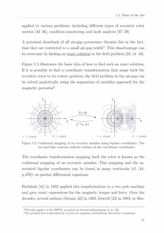
Figure 1.5 illustrates the basic idea of how to find such an exact solution:
If it is possible to find a coordinate transformation that maps back the
eccentric rotor to its centric position, the field problem in the air-gap can
be solved analytically using the separation of variables approach for the
magnetic potential4.
y
x
r = const. θ = const. τ = const. σ = const.
y
x
f(r, θ)
f−1(τ, σ)
Figure 1.5: Conformal mapping of an eccentric annulus using bipolar coordinates. Thered and blue contours indicate isolines of the curvilinear coordinates.
The coordinate transformation mapping back the rotor is known as the
conformal mapping of an eccentric annulus. This mapping and the as-
sociated bipolar coordinates can be found in many textbooks (cf. [44,
p.476]) on partial differential equations.
Buchholz [41] in 1933 applied this transformation to a two pole machine
and gave exact expressions for the magnetic torque and force. Over the
decades, several authors (Swann [42] in 1963, Dorrell [23] in 1993, or Sku-
3This also applies to the MWFA, as proven by Serrano-Iribarnegaray et al. [40].4The problem here is described by a Laplace equation, derived from Maxwell’s equations.
11
1 Introduction
bov and Shumakovich [43] in 1999) have applied it to different machine
types and problems. Dorrell [23, p.139] pointed out, that differences in
the results between the exact solution and air-gap permeance theories
for common machines are rather small. Furthermore he noted, that the
evaluation of the exact solution has to be carried out numerically. Later
in 2017, Boy and Hetzler [45] derived exact expressions for the integrals
occurring in the solution based on a recursive sequence. However, it was
found that the solution is an unstable fixed point of this sequence, making
it unsuitable for inductance calculations.
Another possibility to derive an approximation to the air-gap field pro-
blem is based on an asymptotic expansion. Such an approximation ne-
cessitates a small parameter ε to expand the original field problem into a
series (cf. Nayfeh [46, p.9]).
In 1998 Kim and Lieu [47] used the relation ε = eδ0
between the rotor
eccentricity e and the nominal air-gap length δ0 to derive such an expan-
sion. Their analysis was focused on permanent magnet motors, but can
be applied very generally. Advantages of this method are that the invol-
ved approximation error can be quantified and also further reduced using
higher order approximations. Moreover, it is not necessary to neglect the
non-linear material behaviour of the solids, as the approximation con-
cerns the air-gap only.
Boy and Hetzler [48] proposed a similar method in 2018 using ε = δ0R2
as
a small parameter (R2 is the rotor radius). This modification offers the
advantage, that the approximation is based only on geometrical parame-
ters instead of the dynamic variable e(t). Thus, the approximation quality
of the proposed method does not change due to the rotor motion. The
authors stated their result in terms of a scalar magnetic potential, from
which it was simple to derive both the radial and tangential flux density
components and the magnetic force. As a main finding it turned out, that
12
1.1 State of the Art
the first order approximation (order O(1)) in this method is consistent
with the air-gap permeance theories, but includes an expression for the
tangential field component. Using higher approximation orders (O(ε) and
higher), it has been shown that the solution could be refined. However,
it should be noted that the involved expressions for these higher order
approximations may become lengthy and cumbersome to evaluate.
Several approaches have been proposed to consider saliency and slotting
effects in analytical methods. For the air-gap permeance theories, it is
possible to modulate the permeance to account for such effects. Carter
[49] has shown how to regard this influence by calculating an equivalent
(increased) air-gap width. Using a conformal mapping it is possible to
derive the precise harmonics stemming from the air-gap width variations
(cf. Heller and Hamata [50, p. 60]). Other approaches [51–53] use a sub-
domain decomposition and solve the field problem both in the air-gap
and adjacent regions (slots, permanent magnets etc.).
Numerical Methods
In addition to the potentially lower accuracy, many analytical approa-
ches cannot account for the non-linear magnetic behaviour of the stator
and rotor cores. First attempts to overcome this problem date back to
the 1960s, when the idea of Magnetic equivalent circuits (MEC) was put
forward (cf. Laithwaite [54] in 1967, or Carpenter [55] in 1968). As the
equations in this approach are non-linear, they have to be solved nume-
rically.
Starting from the textbook example of a classical magnetic circuit, equi-
valent networks analogous to electrical circuits are introduced (figure 1.6
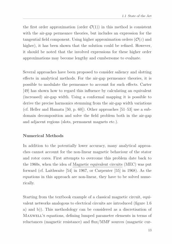
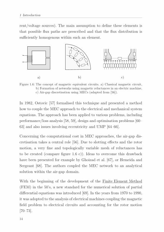
a) and b)). This methodology can be considered as a discretisation of
Maxwell’s equations, defining lumped parameter elements in terms of
reluctances (magnetic resistance) and flux/MMF sources (magnetic cur-
13
1 Introduction
rent/voltage sources). The main assumption to define these elements is
that possible flux paths are prescribed and that the flux distribution is
sufficiently homogenous within such an element.
a) b) c)
Figure 1.6: The concept of magnetic equivalent circuits. a) Classical magnetic circuit,b) Formation of networks using magnetic reluctances in an electric machine,c) Air-gap discretisation using MECs (adapted from [56]).
In 1982, Ostovic [57] formalised this technique and presented a method
how to couple the MEC approach to the electrical and mechanical system
equations. The approach has been applied to various problems, including
performance/loss analysis [58, 59], design and optimisation problems [60–
63] and also issues involving eccentricity and UMP [64–66].
Concerning the computational cost in MEC approaches, the air-gap dis-
cretisation takes a central role [56]. Due to slotting effects and the rotor
motion, a very fine and topologically variable mesh of reluctances has
to be created (compare figure 1.6 c)). Ideas to overcome this drawback
have been presented for example by Ghoizad et al. [67], or Hemeida and
Sergeant [68]. The authors coupled the MEC network to an analytical
solution within the air-gap domain.
With the beginning of the development of the Finite Element Method
(FEM) in the 50’s, a new standard for the numerical solution of partial
differential equations was introduced [69]. In the years from 1970 to 1990,
it was adopted to the analysis of electrical machines coupling the magnetic
field problem to electrical circuits and accounting for the rotor motion
[70–73].
14
1.1 State of the Art
Today the FEM has to be considered as one of the most frequently applied
approaches to account for eccentricity and magnetic forces in electrical
machines. Consequently, there is a very large variety of publications on
these issues including the analysis of different types of motion, design
aspects, or condition monitoring and fault analysis (cf. [74–82]).
From a computational point of view, the FEM implies the same draw-
backs as when using magnetic equivalent circuits. The air-gap region has
to be resolved very finely and for simulations involving eccentricity the
mesh either has to be deformable or remeshed in each time step [83]. As
for the MEC approach, there are methods to couple the FEM to an ana-
lytical solution in the air-gap (cf. [84, 85]).
An overview on the formation of magnetic forces in cage induction ma-
chines and their dependency on different modelling and design aspects
was published by Arkkio et al. [86] in 2000. They used FEM simulations
and compared them to experiments. In their tests, they measured the
lateral magnetic force in an induction machine equipped with magnetic
bearings. In order to understand the relation between displacement and
force, they controlled the lateral motion with the bearings. With this me-
thod they were able to prescribe a circular orbital path with a precisely
defined whirling frequency.
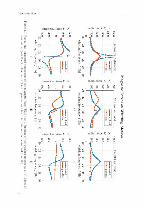
Figure 1.7 shows some results of these simulations. Here, the UMP com-
ponents radial and tangential to the rotor orbit are depicted as functions
of the lateral whirling frequency. Figures a) and b) show the influence of
considering magnetic saturation, c) and d) the effect of load and e) and
f) the change due to different winding designs (parallel branches) at the
stator. Besides revealing that the force depends on various modelling and
design aspects, they also related the formation of forces to the presence
of eccentricity harmonics bp±1 in the air-gap field (as Fruchtenicht et al.
[20] had pointed out).
15
1 Introduction
Figu
re1.7:
Rad
ialan
dtan
gential
compon
entof
themagn
eticforce
(UMP)as
afunction
ofthewhirlin
gfreq
uency.
a)-b)Effect
ofsatu
ration,c)-d
)Effect
ofload
,e)-f)
Effect
ofparallel
bran
ches.
Thedata
has
been
extracted
from[86].
16
1.1 State of the Art
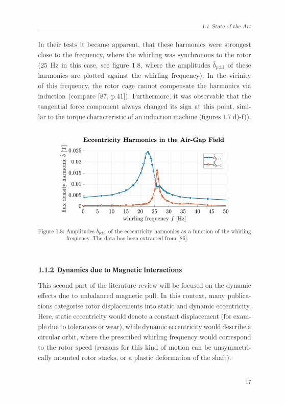
In their tests it became apparent, that these harmonics were strongest
close to the frequency, where the whirling was synchronous to the rotor
(25 Hz in this case, see figure 1.8, where the amplitudes bp±1 of these
harmonics are plotted against the whirling frequency). In the vicinity
of this frequency, the rotor cage cannot compensate the harmonics via
induction (compare [87, p.41]). Furthermore, it was observable that the
tangential force component always changed its sign at this point, simi-
lar to the torque characteristic of an induction machine (figures 1.7 d)-f)).
Figure 1.8: Amplitudes bp±1 of the eccentricity harmonics as a function of the whirlingfrequency. The data has been extracted from [86].
1.1.2 Dynamics due to Magnetic Interactions
This second part of the literature review will be focused on the dynamic
effects due to unbalanced magnetic pull. In this context, many publica-
tions categorise rotor displacements into static and dynamic eccentricity.
Here, static eccentricity would denote a constant displacement (for exam-
ple due to tolerances or wear), while dynamic eccentricity would describe a
circular orbit, where the prescribed whirling frequency would correspond
to the rotor speed (reasons for this kind of motion can be unsymmetri-
cally mounted rotor stacks, or a plastic deformation of the shaft).
17
1 Introduction
Within this work, mainly dynamic orbital motions are analysed. This
means, that in contrast to the prescribed movements in the previously
mentioned categorisation, the lateral displacement of the rotor has to be
calculated here. In this sense, the orbital shape is not known apriori, but
has to be calculated in the same manner as the electrical currents and
the rotational motion are. In the following, this arbitrary orbital motions
will be denoted as ’rotordynamic’, extending the classical categorisation
of static and dynamic eccentricities by an additional type of motion. Fo-
cusing the discourse on such rotordynamic aspects in this work, issues
like condition monitoring and failure analysis will not be addressed in the
following.
The first and most profound insight on dynamic aspects is that the ma-
gnetic force may reduce the critical bending speed [14]. This is due to
the fact, that for many operational conditions the radial UMP points
outwards to the direction of the smallest air-gap (figure 1.4) and will in-
crease with the radial rotor displacement. In a first order approximation
and for constant flux operation, this part of the magnetic force can be
interpreted as a negative mechanical spring5.
In a review paper from 1968, Ellison and Moore [88] have summarised
earlier findings on rotor vibrations. They stated that the rotor response
to most magnetic force waves is small except for those which travel at the
critical speed of the rotor. Besides the fundamental, they mentioned the
effect of slotting harmonics, subharmonics of the MMF and field waves
caused by parallel branches. Considering gyroscopic effects, they claimed
that the rotor behaviour may be complex [88].
Besides that, it has become apparent in the preceding discussion that
there are many factors of influence changing both the magnitude and the
5Note that the concept of a negative mechanical spring drastically oversimplifies the underlying phy-sics. In sections 2.2.4 and 2.6 more precise definitions of the UMP are given.
18
1.1 State of the Art
direction of the UMP. Thus, it is obvious that very different kinds of rotor
oscillations may occur (think of self-excited oscillations as an example).
Moreover, the dynamic coupling between lateral motion and electrical
currents may come into play and as it is inherently non-linear, it may
couple different vibration phenomena (for example due to synchronisati-
on).
Asynchronous Machines
In 1982 Fruchtenicht et al. [20, 89] published two papers, where they deri-
ved a magnetic force model (compare section 1.1.1) based on the air-gap
permeance method. They focused the analysis to the harmonic orders
p and p ± 1 of the air-gap field and assumed that the rotational speed
is constant. Combining this model with a Laval/Jeffcott rotor (cf.
Gasch et al. [7]), they analysed self-excited rotor vibrations. A major
assumption on the motion was, that the orbit would always be circular
and that the whirling frequency would correspond to the rotor speed. Ac-
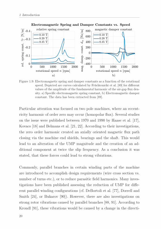
cording to their explanation, the induction to the rotor cage caused an
electromagnetic damping force, which could become negative at certain
speeds (compare figure 1.9). If this negative damping exceeded the value
of the (positive) mechanical damping, strong oscillations would occur.
They validated their model experimentally using a particularly modified
test machine, where they varied the speed by changing the slip.
Werner [87] in 2006 extended the model of Fruchtenicht et al. towards
elliptical orbits, which can be interpreted as a superposition of circular
forward and backward motions. He investigated magnetic forces due to
different orbit frequencies and came to the conclusion that for the cases
considered in his work only vibrations corresponding to the rotor fre-
quency were of interest. In his analysis he investigated the influence of
different bearing types. Using finite element simulation, he examined the
boundaries of validity for the analytical model and considered saturation
effects.
19
1 Introduction
Figure 1.9: Electromagnetic spring and damper constants as a function of the rotationalspeed. Depicted are curves calculated by Fruchtenicht et al. [89] for differentvalues of the amplitude of the fundamental harmonic of the air-gap flux den-sity. a) Specific electromagnetic spring constant, b) Electromagnetic damperconstant. The data has been extracted from [89].
Particular attention was focused on two pole machines, where an eccent-
ricity harmonic of order zero may occur (homopolar flux). Several studies
on the issue were published between 1970 and 1990 by Haase et al. [17],
Kovacs [18] and Belmans et al. [21, 22]. According to their investigations,
the zero order harmonic created an axially oriented magnetic flux path
closing via the machine end shields, bearings and the shaft. This would
lead to an alteration of the UMP magnitude and the creation of an ad-
ditional component at twice the slip frequency. As a conclusion it was
stated, that these forces could lead to strong vibrations.
Commonly, parallel branches in certain winding parts of the machine
are introduced to accomplish design requirements (wire cross section vs.
number of turns etc.), or to reduce parasitic field harmonics. Many inves-
tigations have been published assessing the reduction of UMP for diffe-
rent parallel winding configurations (cf. DeBortoli et al. [77], Dorrell and
Smith [24], or Bukarov [90]). However, there are also investigations on
strong rotor vibrations caused by parallel branches [88, 91]. According to
Krondl [91], these vibrations would be caused by a change in the directi-
20
1.1 State of the Art
on of the UMP due to induction. He investigated different configurations,
both for parallel branches in slip ring rotors and stator windings and de-
rived analytical frequency response curves for the magnetic force. Thus,
he was able to assess the rotordynamic behaviour by defining magnetic
spring and damper constants.
Arkkio et al. [86] showed, that saturation has a strong effect on the UMP
(see also figures 1.7 a) and b)). Based on their measurements and finite
element simulations they developed a low-order model allowing them to
take into account various influence factors like slotting, saturation and
parallel branches. They extended the model of Fruchtenicht et al. by de-
fining a complex frequency response function for the magnetic force. The
model parameters had been adjusted to the results from finite element
simulations. For real valued parameters, their model and the approach
by Fruchtenicht et al. were in accordance. Major assumptions associated
with their model concerned the operation at stationary speed and a linear
relation between the magnetic forces and the rotor displacement.
Beyond several extensions to this idea (cf. [90, 92]), Holopainen [93] in
2005 modified the approach to account for arbitrary orbital motions in
the sense of rotordynamics and transient states. Compared to the former
model, he included two additional dynamic variables for higher harmo-
nics of the currents in the rotor cage. Thus, the approach considered a
full coupling between the mechanical motion and the harmonic currents.
As a main result he showed that the interaction may decrease the natural
frequency, cause additional dissipation, or even self-excited oscillations.
The effects were observed to be particularly strong, when operating close
to the first critical bending speed.
In a later review paper from 2008, Holopainen and Arkkio [94] concluded
that when evaluating self-excited oscillations, a linear approach based on
magnetic spring and damper coefficients might not be sufficient in or-
21
1 Introduction
der to capture all possible phenomena. They confirmed this statement by
showing measurements involving non-linear limit cycle oscillations of the
rotor in a cage induction machine.
Boy and Hetzler [95] in 2017 investigated the force-displacement relati-
on proposed by Fruchtenicht et al. and its dynamic consequences. They
derived from quasi-stationary Maxwell’s equations that tangential ma-
gnetic forces have to be considered as electromagnetic circulatory forces
(cf. Merkin [96, p.160]), i.e. non-conservative positional forces. The ve-
locity proportional ’damping’ forces by Fruchtenicht et al. [20] had been
obtained due to the initial requirement of a prescribed orbit, where the
eccentricity was assumed to be constant. Thus, they identified an equiva-
lent damping constant from the tangential force. Since non-conservative
positional forces may lead to a totally different dynamic behaviour than
velocity proportional forces (as damping forces are), the replacement may
not capture the dynamics correctly. Boy and Hetzler illustrated their fin-
dings by comparing stability threshold speeds calculated using both the
positional and the velocity dependent force models.
Further rotordynamic investigations have been presented by Skubov and
Shumakovich [43], who used Lagrange-Maxwell equations to derive
a non-linear fully coupled model. They focused the analysis on the fun-
damental harmonic of the air-gap field and excluded saturation effects.
To solve the magnetic field problem they utilised a conformal mapping
approach. Laiho et al. [97] presented a method to control lateral rotor
oscillations and Mair et al. [98] developed a model including the hetero-
genous rotor assembly using Timoshenko beam elements. They observed
higher harmonics in the rotor response due to magnetic forces.
22
1.1 State of the Art
Synchronous Machines
In synchronous machines without damper windings and parallel branches,
the reduction of the critical bending speed is often larger than in cage in-
duction machines. This is due to the fact, that the eccentricity waves
cannot be damped by circulating currents (cf. Brown et al. [99]). Beyond
that, there are several additional phenomena reported in the literature,
which will be summarised in the following.
In 1966 Kellenberger [8] observed strong vibrations in a two-pole turbo-
generator. He stated an analytical model of the UMP, where he varied the
force amplitude and direction depending on the orientation between the
pole axis and the eccentric displacement. Combining this model with the
classical Laval/Jeffcott rotor, he found a splitting of the first critical
bending speed and a region of instability in between. Boy and Hetzler
[100] showed, that this model leads to a dynamic behaviour similar to the
effect of a non-circular shaft (compare [7, p.383]).
Kim et al. [101] compared the effect of magnetic forces on dynamic orbits
of permanent magnet machines. Based on transient finite element simula-
tions, they compared interior and surface mount designs and found, that
in their case, the machine with interior magnets exhibited much larger
oscillations.
Guo et al. [102] developed a simplified force model for generators. Ne-
glecting any effect due to induction and saturation by prescribing the
magnetomotive force, they analysed the effect of magnetic forces on the
rotor orbital motion. For larger eccentricities, they found considerable
deviations from the initially circular shapes including more than one os-
cillation frequency.
Lundstrom and his co-authors published several papers (cf. [103–105])
23
1 Introduction
concerning the rotordynamics of hydropower generators. Using both fini-
te element simulations and analytical models, they investigated the influ-
ence of damper windings and shape deviations of the rotor surface and
stator bore. They found that damper windings may cause a tangential
force component and thus lead to strong vibrations. For the shape de-
viations they were able to show that the resulting magnetic forces could
excite both forward and backward orbits and thus lead to a more complex
dynamic behaviour.
Pennacchi [106] in 2008 presented a model describing the dynamics of
generators. Based on the air-gap permeance he calculated the UMP and
combined it with a finite element rotor model. His force expressions were
derived for arbitrary orbital motions. In his analysis, he found forces of
different frequencies and a resulting non-circular orbital shape. He assi-
gned his observations to the non-linearity of the UMP.
Im et al. [107] investigated the rotordynamics of a Brushless DC motor.
They derived a non-linear fully coupled model based on the Lagrange-
Maxwell equations. The magnetic forces were derived using the air-gap
permeance, thus neglecting saturation effects. As a major result they
stated that the eccentric motion would have a weak effect on the electric
currents and the machine torque.
In 2016, Xiang et al. [108] published a rotordynamic investigation of per-
manent magnet motors. They calculated the magnetic forces using the air-
gap permeance and neglected saturation effects. Prescribing the magneto-
motive force, no electrical dynamics were regarded. In their analysis, they
found a softening non-linear stiffness behaviour due to the UMP and re-
ported of non-linear interactions between forward and backward whirling
motions.
24
1.2 Aims and Structure of the Work
1.2 Aims and Structure of the Work
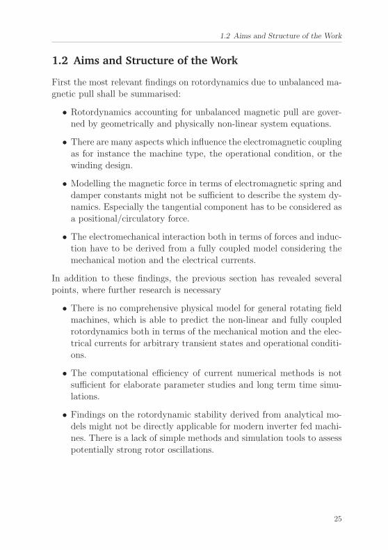
First the most relevant findings on rotordynamics due to unbalanced ma-gnetic pull shall be summarised:
• Rotordynamics accounting for unbalanced magnetic pull are gover-ned by geometrically and physically non-linear system equations.
• There are many aspects which influence the electromagnetic couplingas for instance the machine type, the operational condition, or thewinding design.
• Modelling the magnetic force in terms of electromagnetic spring anddamper constants might not be sufficient to describe the system dy-namics. Especially the tangential component has to be considered asa positional/circulatory force.
• The electromechanical interaction both in terms of forces and induc-tion have to be derived from a fully coupled model considering themechanical motion and the electrical currents.
In addition to these findings, the previous section has revealed severalpoints, where further research is necessary
• There is no comprehensive physical model for general rotating fieldmachines, which is able to predict the non-linear and fully coupledrotordynamics both in terms of the mechanical motion and the elec-trical currents for arbitrary transient states and operational conditi-ons.
• The computational efficiency of current numerical methods is notsufficient for elaborate parameter studies and long term time simu-lations.
• Findings on the rotordynamic stability derived from analytical mo-dels might not be directly applicable for modern inverter fed machi-nes. There is a lack of simple methods and simulation tools to assesspotentially strong rotor oscillations.
25
1 Introduction
These academic voids motivate the statement of the following aims forthis thesis:
• Aim 1: Deriving a fully coupled two dimensional6 physical model,describing the rotordynamics and electrical currents of general ro-tating field machines. The model is supposed to consider both geo-metrical and physical non-linearities, as well as arbitrary windingdesigns and transient operational conditions. The approach shouldprovide for sufficient computational efficiency in order to run longterm simulations and large parameter studies.
• Aim 2: Proving the validity of the developed model by comparisonto well established analytical and numerical methods and publishedexperimental results.
• Aim 3: Using the model to demonstrate its suitability for rotordy-namic analysis. Based on the simulation results, simple methods forthe assessment of self-excited rotor oscillations shall be deduced.
Following these aims, this thesis is organised as follows: in chapter 2, the
model will be established. To accomplish this, first the physical problem
is stated and an overview on the basic governing equations is provided.
Second, the fundamental structure of the electromechanical system equa-
tions for coupled dynamic problems is reviewed. Here, different approa-
ches for the derivation of the equations of motion in terms of Newton-
Faraday and Lagrange-Maxwell equations are discussed and com-
pared. Next, approaches to model the three subproblems in terms of the
mechanical part, the electrical circuits and the magnetic field problem
are presented. Subsequently, particular focus is set on the electromecha-
nical coupling in terms of the magnetic torque, forces and induction and
the equivalence between the coupling for the Newton-Faraday and
Lagrange-Maxwell equations is proven. Finally, the complete set of
equations is summarised and the computational implementation using
MATLAB is outlined.
6The term two dimensional refers to the two dimensional (lateral) rotor motion and the magneticfield, where axial effects are not considered.
26
1.2 Aims and Structure of the Work
Chapter 3 deals with the validation of the proposed model. Here, ex-
amples of a 50 kW 4-pole cage induction machine (E-FFEKT prototype
[109]) and a 60 kW 8-pole interior permanent magnet synchronous ma-
chine (2010 Toyota Prius traction drive [110]) are considered. The vali-
dation for both examples is carried out in two steps: first, the magnetic
field, torque and forces are compared to finite element simulations and
measurements. Second, the dynamic behaviour is validated with space
vector models of both machine types.
In chapter 4 simulation studies for the example machines from chapter
3 are presented. For the cage induction machine, critical speeds for self-
excited oscillations are investigated. For the synchronous motor, both the
effect of a static rotor offset, as well as self-excitation due to parallel bran-
ches will be analysed. In both cases, the observations are used to deduce
simple and general statements, allowing the assessment of the occurence
of potentially dangerous magnetic excited rotor oscillations.
Chapter 5 summarises the work and draws some conclusions. At the end
an outlook on further research will be given.
This thesis is accompanied by four appendix sections, covering fundamen-
tals on electromechanical energy functionals, the asymptotic expansion of
the air-gap magnetic field, some basics on magnetic equivalent circuits and
finally, a summary of the machine and model parameters for the examples
in chapters 3 and 4.
27
2 Model
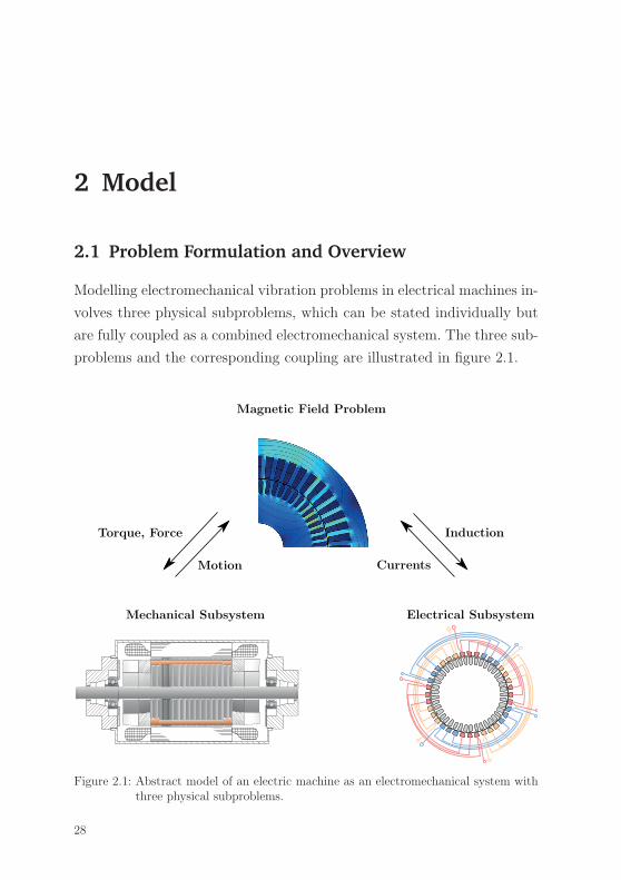
2.1 Problem Formulation and Overview
Modelling electromechanical vibration problems in electrical machines in-
volves three physical subproblems, which can be stated individually but
are fully coupled as a combined electromechanical system. The three sub-
problems and the corresponding coupling are illustrated in figure 2.1.
Mechanical Subsystem Electrical Subsystem
Magnetic Field Problem
Induction
Currents
Torque, Force
Motion
Figure 2.1: Abstract model of an electric machine as an electromechanical system withthree physical subproblems.
28
2.1 Problem Formulation and Overview
In the following, the mechanical subsystem shall consist of all moving
parts in the machine, comprising for example the rotor and shaft, as well
as the bearing arrangement. The aim of modelling this part is to describe
the motion of these components in terms of rotation and lateral displa-
cements. The magnetic field affects the motion by exerting torque and
forces.
The electrical subsystem is formed of all conducting elements, which
are arranged on the stator and rotor of the machine. The dynamic varia-
bles in this subsystem are the currents flowing through the conducters.
The time changing magnetic field couples to the electrical subsystem by
inducing voltage to the electrical circuits.
Describing the magnetic field represents the third and last subproblem.
This field mediates the electromechanical interaction through the air gap
of the machine. It is affected by the mechanical motion, as the rotational
and lateral displacement of the rotor modify the geometry of the air-gap
and distort the flux lines. Furthermore it directly depends on the electrical
subsystem, as the currents are sources to it. Note that there is no direct
coupling between the mechanical and the electrical subsystem. Therefore,
all interactions are transmitted by the magnetic field.
2.1.1 Governing Equations
Casting the considered physical problem into mathematical equations can
be handled in two formally different, but physically equivalent ways. In
the context of classical dynamics fundamental axioms in terms of New-
ton’s and Euler’s laws of motion and Maxwell’s equations of electro-
dynamics are stated. These laws have to be accompanied by constitutive
relations closing the equation system. Alternatively, energy based approa-
ches in the context of analytical dynamics can be used employing varia-
tional principles. Here, Hamilton’s principle will be considered since it
29
2 Model
offers a common framework to handle both mechanics and electrodyna-
mics simultanously. In this second class of approaches, the constitutive
equations are incorporated in the energy functionals stated to derive the
governing equations.
Regarding the mathematical structure both approaches do have a very
different character: while classical dynamics describe the time and space
evolution of the system by means of differential equations, analytical me-
thods express a kind of underlying principle of the dynamics of a system.
These principles state that among all possible evolutions the system will
follow the particular dynamics that renders a certain scalar quantity (for
example an action integral) extremal.
For electrical machines, the classical approach is more common today. Ho-
wever, analytical methods offer several advantages: being energy based, it
is possible to formulate both the mechanical motion and the electrodyna-
mics in one principle. This allows to model electromechanical interactions
inherently energy consistent and greatly simplifies the analysis. Further-
more, the special choice of variables in analytical approaches reduces the
number of equations which have to be solved to a minimum. In this work,
the governing equations will be established in both ways and both approa-
ches will be compared. The equivalence of the methods will be shown and
implications for approximations made while establishing the model will
be analysed.
Classical Dynamics
Mathematically, classical dynamics is expressed in terms of differential
equations. The mechanical motion of a body B (cf. figure 2.2 a)) is
determined by the balance equations of linear and angular momentum
(Newton’s and Euler’s laws) reading
30
2.1 Problem Formulation and Overview
d�p
dt= �f, where �p =
∫B�v dm, (2.1a)
d�� (P )
dt= �τ (P ), where �� (P ) =
∫B�r × �v dm. (2.1b)
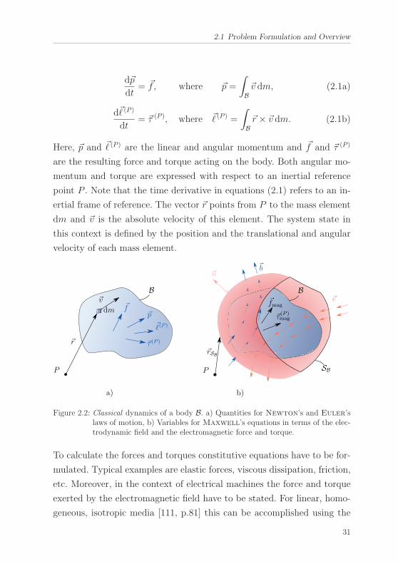
Here, �p and �� (P ) are the linear and angular momentum and �f and �τ (P )
are the resulting force and torque acting on the body. Both angular mo-
mentum and torque are expressed with respect to an inertial reference
point P . Note that the time derivative in equations (2.1) refers to an in-
ertial frame of reference. The vector �r points from P to the mass element
dm and �v is the absolute velocity of this element. The system state in
this context is defined by the position and the translational and angular
velocity of each mass element.
a) b)
P
dm
�vB
�p�f
��(P )
�τ (P )�r
P
B
�rSB
SB
�n�b
�e�fmag
�τ(P )mag
Figure 2.2: Classical dynamics of a body B. a) Quantities for Newton’s and Euler’slaws of motion, b) Variables for Maxwell’s equations in terms of the elec-trodynamic field and the electromagnetic force and torque.
To calculate the forces and torques constitutive equations have to be for-
mulated. Typical examples are elastic forces, viscous dissipation, friction,
etc. Moreover, in the context of electrical machines the force and torque
exerted by the electromagnetic field have to be stated. For linear, homo-
geneous, isotropic media [111, p.81] this can be accomplished using the
31
2 Model
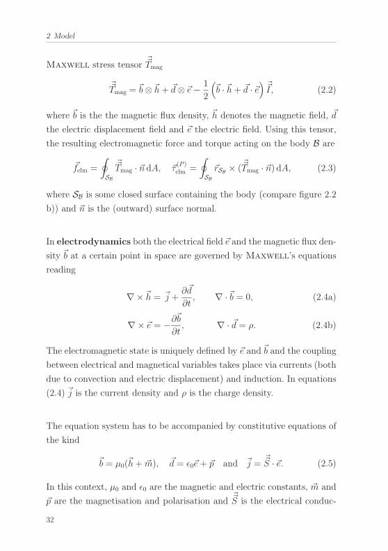
Maxwell stress tensor��Tmag
��Tmag = �b⊗ �h+ �d⊗ �e− 1
2
(�b · �h+ �d · �e
)��I, (2.2)
where �b is the the magnetic flux density, �h denotes the magnetic field, �d
the electric displacement field and �e the electric field. Using this tensor,
the resulting electromagnetic force and torque acting on the body B are
�felm =
∮SB
��Tmag · �n dA, �τ(P )elm =
∮SB�rSB × (
��Tmag · �n) dA, (2.3)
where SB is some closed surface containing the body (compare figure 2.2
b)) and �n is the (outward) surface normal.
In electrodynamics both the electrical field �e and the magnetic flux den-
sity �b at a certain point in space are governed by Maxwell’s equations
reading
∇× �h = �j +∂ �d
∂t, ∇ ·�b = 0, (2.4a)
∇× �e = −∂�b
∂t, ∇ · �d = ρ. (2.4b)
The electromagnetic state is uniquely defined by �e and �b and the coupling
between electrical and magnetical variables takes place via currents (both
due to convection and electric displacement) and induction. In equations
(2.4) �j is the current density and ρ is the charge density.
The equation system has to be accompanied by constitutive equations of
the kind
�b = μ0(�h+ �m), �d = ε0�e+ �p and �j =��S · �e. (2.5)
In this context, μ0 and ε0 are the magnetic and electric constants, �m and
�p are the magnetisation and polarisation and��S is the electrical conduc-
32
2.1 Problem Formulation and Overview
tivity tensor. Especially �m and �p have to be individually formulated in
(non-linear) dependence of �e and �b for each considered material.
The mechanical motion affects the electromagnetic fields by changing the
shape and location of of the considered body. A typical effect in this
context, which will become relevant later, is the motional induction. Alt-
hough not mentioned in detail here, both the mechanical problem, as well
as the electromagnetic equations require boundary and initial conditions
to solve them (cf. [111, p.61]).
Analytical Dynamics
Different to classical dynamics, analytical (also called energetical, varia-
tional, or indirect) approaches are not based on the direct statement of
differential equations in time and space. Instead, they are based on fun-
damental principles, which state that the solution of a system will evolve
such that some scalar functional (a function of the motion and fields) will
be brought to an extremum.
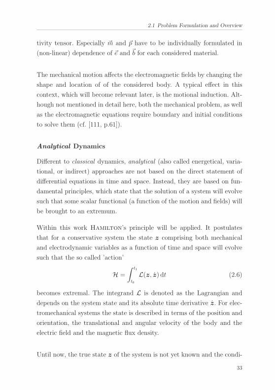
Within this work Hamilton’s principle will be applied. It postulates
that for a conservative system the state z comprising both mechanical
and electrodynamic variables as a function of time and space will evolve
such that the so called ’action’
H =
∫ t1
t0
L(z, z) dt (2.6)
becomes extremal. The integrand L is denoted as the Lagrangian and
depends on the system state and its absolute time derivative z. For elec-
tromechanical systems the state is described in terms of the position and
orientation, the translational and angular velocity of the body and the
electric field and the magnetic flux density.
Until now, the true state z of the system is not yet known and the condi-
33
2 Model
tion of extremality still has to be expressed mathematically. This can be
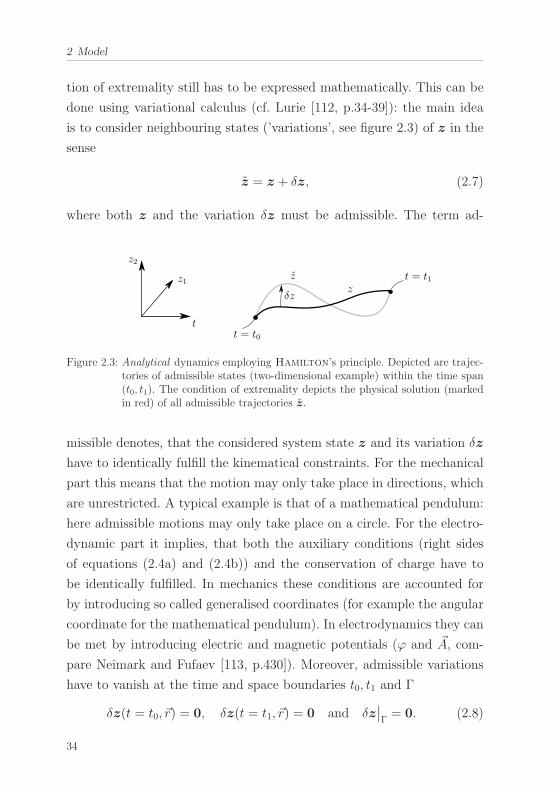
done using variational calculus (cf. Lurie [112, p.34-39]): the main idea
is to consider neighbouring states (’variations’, see figure 2.3) of z in the
sense
z = z + δz, (2.7)
where both z and the variation δz must be admissible. The term ad-
t
z1
z2
t = t0
t = t1z
z
δz
Figure 2.3: Analytical dynamics employing Hamilton’s principle. Depicted are trajec-tories of admissible states (two-dimensional example) within the time span(t0, t1). The condition of extremality depicts the physical solution (markedin red) of all admissible trajectories z.
missible denotes, that the considered system state z and its variation δz
have to identically fulfill the kinematical constraints. For the mechanical
part this means that the motion may only take place in directions, which
are unrestricted. A typical example is that of a mathematical pendulum:
here admissible motions may only take place on a circle. For the electro-
dynamic part it implies, that both the auxiliary conditions (right sides
of equations (2.4a) and (2.4b)) and the conservation of charge have to
be identically fulfilled. In mechanics these conditions are accounted for
by introducing so called generalised coordinates (for example the angular
coordinate for the mathematical pendulum). In electrodynamics they can
be met by introducing electric and magnetic potentials (ϕ and �A, com-
pare Neımark and Fufaev [113, p.430]). Moreover, admissible variations
have to vanish at the time and space boundaries t0, t1 and Γ
δz(t = t0, �r) = 0, δz(t = t1, �r) = 0 and δz∣∣Γ= 0. (2.8)
34
2.1 Problem Formulation and Overview
Substituting equation (2.7) into Hamilton’s principle (2.6) yields
H(z, ˙z) = H(z, z) + δH(z, z) +O(δ2H) (2.9)
for sufficiently smooth integrands L. From this it follows that H(z, z) will
only be extremal – and thus z will be the solution – if
δH(z, z) = 0. (2.10)
This equation governs the dynamics of potential systems. The principle
may be generalised to
δH(z, z, t) +
∫ t1
t0
δWnp(z, z, t) dt = 0, (2.11)
where δWnp is the so called virtual work performed by all components
(forces, voltages etc.), which are not accounted for in an energy potential
(for example external, or dissipative forces, or external voltages and oh-
mic resistances). This distinction has to be made, as there may not exist
potential expressions for all system components.
The axiomatic equations (2.1) and (2.4) are contained in equation (2.6)
and can be exactly deduced by computing the variation (cf. [114, p.22-
33], or [113, p.431-435]). However, there are two important differences bet-
ween classical and analytical approaches: first, the definition of admissible
state variables automatically fulfills kinematical constraints, reducing the
number of variables (and equations) to solve for. Second, the constitutive
equations are already included in L and Wnp. Therefore, expressions for
the electromagnetic torque and forces, as well as for motional effects on
the electromagnetic field can all be derived from these functionals and
are automatically energy consistent.
The precise definition of L and δW depends on the type of problem
considered. They will be given for a lumped parameter model in the
subsequent section. For continuous problems refer to Neımark and Fufaev
[113, p.426-435]. An overview on the basic definition of energy functionals
is given in appendix A.
35
2 Model
2.1.2 Fundamental Assumptions and their Implications
No matter which approach is chosen, the very general equations just men-
tioned have to be simplified and adopted for the actual problem to be
considered. To this end, some fundamental assumptions are made before
continuing with the discussion:
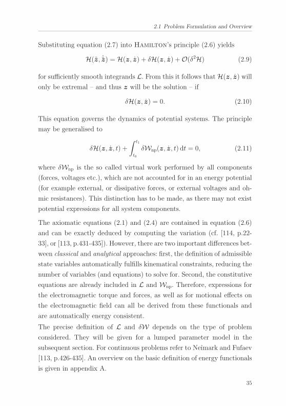
Assumptions 1: Fundamentals
1. All involved bodies having mass are considered rigid. The in-volved speeds are far below the speed of light.
2. The quasi-stationary form of Maxwell’s equations is valid.Electrodynamic effects are not considered.
3. Physical phenomena concerning the mechanical and the elec-trical subsystems can be described by lumped parameter mo-dels.
4. Electrical capacitances are neglected compared to magneticinductances.
5. The electromagnetic material is assumed isotropic. It mayshow non-linear behaviour (saturation) but no hysteresis.
6. All kinematical constraints are holonomic and scleronomous.
7. Thermal effects can be neglected. All considerations are iso-thermal.
Condensation towards Lumped Parameter Equations
Due to assumption 1.1, deformations of the considered body (for ex-
ample the stator housing) are excluded. However, the restriction has two
major consequences: first, the angular velocity �ω is the same for each
point of the body. Second, all velocities of mass elements forming the
body are known, if the velocity �vM of a reference point M is known. This
latter fact can be found when considering some arbitrary point A located
36
2.1 Problem Formulation and Overview
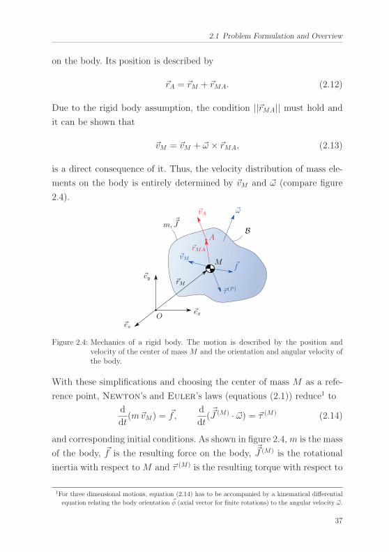
on the body. Its position is described by
�rA = �rM + �rMA. (2.12)
Due to the rigid body assumption, the condition ||�rMA|| must hold and
it can be shown that
�vM = �vM + �ω × �rMA, (2.13)
is a direct consequence of it. Thus, the velocity distribution of mass ele-
ments on the body is entirely determined by �vM and �ω (compare figure
2.4).
O
m,��J B
�f
�τ (P )
�rM
M
�ω
�vM
A
�rMA
�vA
�ex
�ey
�ez
Figure 2.4: Mechanics of a rigid body. The motion is described by the position andvelocity of the center of mass M and the orientation and angular velocity ofthe body.
With these simplifications and choosing the center of mass M as a refe-
rence point, Newton’s and Euler’s laws (equations (2.1)) reduce1 to
d
dt(m�vM) = �f,
d
dt(��J (M) · �ω) = �τ (M) (2.14)
and corresponding initial conditions. As shown in figure 2.4,m is the mass
of the body, �f is the resulting force on the body,��J (M) is the rotational
inertia with respect toM and �τ (M) is the resulting torque with respect to
1For three dimensional motions, equation (2.14) has to be accompanied by a kinematical differential
equation relating the body orientation �φ (axial vector for finite rotations) to the angular velocity �ω.
37
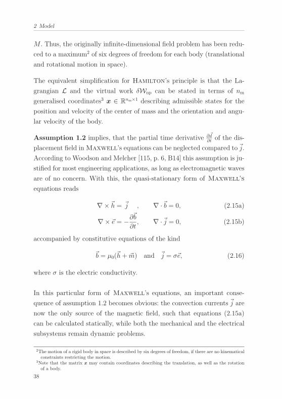
2 Model
M . Thus, the originally infinite-dimensional field problem has been redu-
ced to a maximum2 of six degrees of freedom for each body (translational
and rotational motion in space).
The equivalent simplification for Hamilton’s principle is that the La-
grangian L and the virtual work δWnp can be stated in terms of nm
generalised coordinates3 x ∈ Rnm×1 describing admissible states for the
position and velocity of the center of mass and the orientation and angu-
lar velocity of the body.
Assumption 1.2 implies, that the partial time derivative ∂ �d∂t of the dis-
placement field in Maxwell’s equations can be neglected compared to �j.
According to Woodson and Melcher [115, p. 6, B14] this assumption is ju-
stified for most engineering applications, as long as electromagnetic waves
are of no concern. With this, the quasi-stationary form of Maxwell’s
equations reads
∇× �h = �j , ∇ ·�b = 0, (2.15a)
∇× �e = −∂�b
∂t, ∇ ·�j = 0, (2.15b)
accompanied by constitutive equations of the kind
�b = μ0(�h+ �m) and �j = σ�e, (2.16)
where σ is the electric conductivity.
In this particular form of Maxwell’s equations, an important conse-
quence of assumption 1.2 becomes obvious: the convection currents �j are
now the only source of the magnetic field, such that equations (2.15a)
can be calculated statically, while both the mechanical and the electrical
subsystems remain dynamic problems.
2The motion of a rigid body in space is described by six degrees of freedom, if there are no kinematicalconstraints restricting the motion.
3Note that the matrix x may contain coordinates describing the translation, as well as the rotationof a body.
38
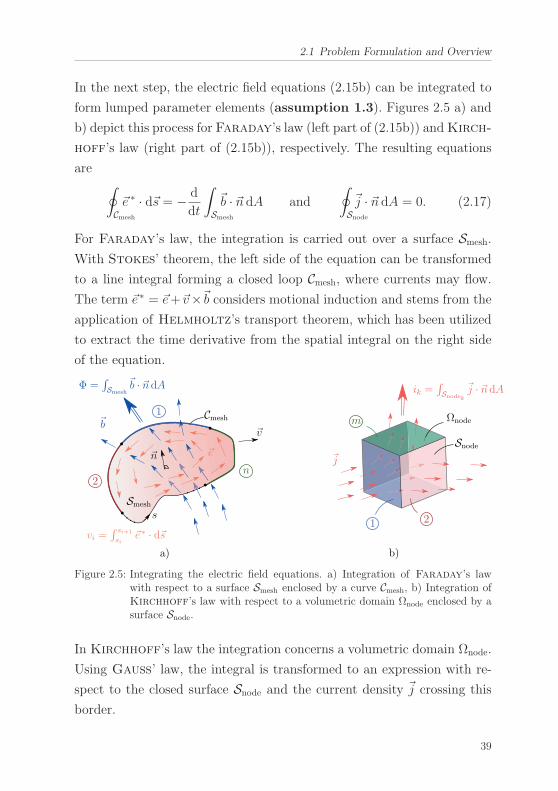
2.1 Problem Formulation and Overview
In the next step, the electric field equations (2.15b) can be integrated to
form lumped parameter elements (assumption 1.3). Figures 2.5 a) and
b) depict this process for Faraday’s law (left part of (2.15b)) andKirch-
hoff’s law (right part of (2.15b)), respectively. The resulting equations
are ∮Cmesh
�e ∗ · d�s = − d
dt
∫Smesh
�b · �n dA and
∮Snode
�j · �n dA = 0. (2.17)
For Faraday’s law, the integration is carried out over a surface Smesh.
With Stokes’ theorem, the left side of the equation can be transformed
to a line integral forming a closed loop Cmesh, where currents may flow.
The term �e ∗ = �e+�v×�b considers motional induction and stems from the
application of Helmholtz’s transport theorem, which has been utilized
to extract the time derivative from the spatial integral on the right side
of the equation.
a) b)
Smesh
Cmesh1
2n
s
�n �e
�b
Φ =∫Smesh
�b · �n dA
vi =∫ si+1
si�e ∗ · d�s
�v
Ωnode
�j
1 2
m
ik =∫Snodek
�j · �n dA
Snode
Figure 2.5: Integrating the electric field equations. a) Integration of Faraday’s lawwith respect to a surface Smesh enclosed by a curve Cmesh, b) Integration ofKirchhoff’s law with respect to a volumetric domain Ωnode enclosed by asurface Snode.
In Kirchhoff’s law the integration concerns a volumetric domain Ωnode.
Using Gauß’ law, the integral is transformed to an expression with re-
spect to the closed surface Snode and the current density �j crossing this
border.
39
2 Model
The integral
Φ =
∫Smesh
�b · �n dA (2.18)
is defined as the magnetic flux Φ passing through the mesh surface Smesh.
In technical systems, the boundary curve Cmesh often encircles the mesh
surface Smesh several times (for example in a coil). If N is the number of
turns then the flux linkage λ is defined as
λ = NΦ = N
∫Smesh
�b · �n dA. (2.19)
The boundaries for both regions in figure 2.5 can be subdivided into
individual sections (index i = 1, ..., n for Cmesh and k = 1, ...,m for Snode).
Through this, discrete voltage drops
vi = −∫Ci�e ∗ · d�s (2.20)
and resulting currents
ik =
∫Sk
�j · �n dA (2.21)
can be defined. The negative sign for the voltage is a convention. Finally,
equations (2.17) become
n∑i=1
vi =dλ
dtand
m∑k=1
ik = 0, (2.22)
accompanied by initial conditions. In the following, the complete set
of Newton’s, Euler’s, Faraday’s and Kirchhoff’s laws (relations
(2.14) and (2.22)) will be abbreviated with the term Newton-Faraday
equations in the context of classical dynamics.
40
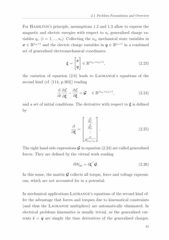
2.1 Problem Formulation and Overview
For Hamilton’s principle, assumptions 1.2 and 1.3 allow to express the
magnetic and electric energies with respect to ne generalised charge va-
riables qi, (i = 1, ..., ne). Collecting the nm mechanical state variables in
x ∈ Rnm×1 and the electric charge variables in q ∈ R
ne×1 in a combined
set of generalised electromechanical coordinates
ξ =
[x
q
]∈ R
(nm+ne)×1, (2.23)
the variation of equation (2.6) leads to Lagrange’s equations of the
second kind (cf. [114, p.302]) reading
d
dt
∂L∂ξ
− ∂L∂ξ
= G ∈ R(nm+ne)×1, (2.24)
and a set of initial conditions. The derivative with respect to ξ is defined
by
∂
∂ξ=
⎡⎢⎢⎢⎢⎣
∂∂ξ1∂∂ξ2...∂
∂ξnm+ne
⎤⎥⎥⎥⎥⎦ . (2.25)
The right hand side expressions G in equation (2.24) are called generalised
forces. They are defined by the virtual work reading
δWnp = δξ�G. (2.26)
In this sense, the matrix G collects all torque, force and voltage expressi-
ons, which are not accounted for in a potential.
In mechanical applications Lagrange’s equations of the second kind of-
fer the advantage that forces and torques due to kinematical constraints
(and thus the Lagrange multipliers) are automatically eliminated. In
electrical problems kinematics is usually trivial, as the generalised cur-
rents i = q are simply the time derivatives of the generalised charges.
41
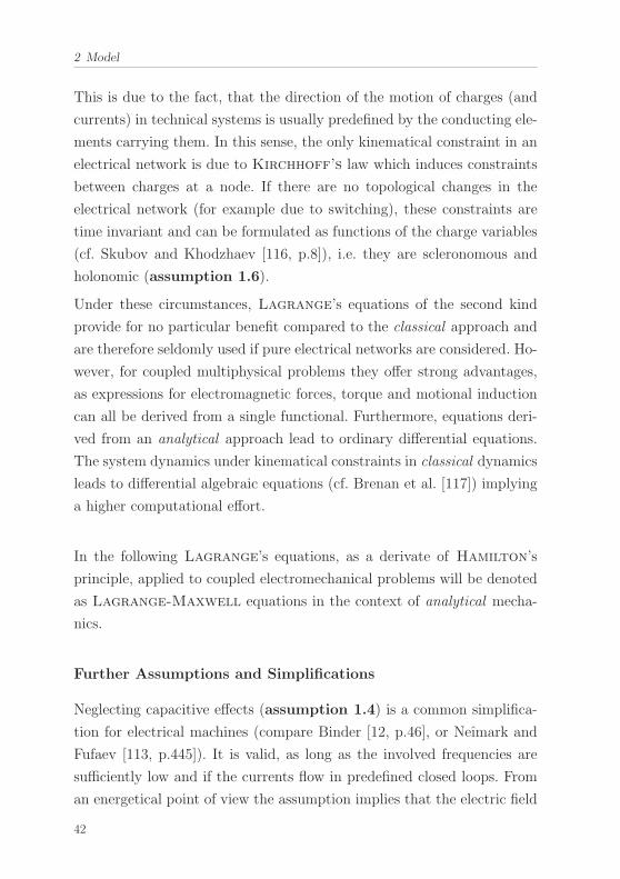
2 Model
This is due to the fact, that the direction of the motion of charges (and
currents) in technical systems is usually predefined by the conducting ele-
ments carrying them. In this sense, the only kinematical constraint in an
electrical network is due to Kirchhoff’s law which induces constraints
between charges at a node. If there are no topological changes in the
electrical network (for example due to switching), these constraints are
time invariant and can be formulated as functions of the charge variables
(cf. Skubov and Khodzhaev [116, p.8]), i.e. they are scleronomous and
holonomic (assumption 1.6).
Under these circumstances, Lagrange’s equations of the second kind
provide for no particular benefit compared to the classical approach and
are therefore seldomly used if pure electrical networks are considered. Ho-
wever, for coupled multiphysical problems they offer strong advantages,
as expressions for electromagnetic forces, torque and motional induction
can all be derived from a single functional. Furthermore, equations deri-
ved from an analytical approach lead to ordinary differential equations.
The system dynamics under kinematical constraints in classical dynamics
leads to differential algebraic equations (cf. Brenan et al. [117]) implying
a higher computational effort.
In the following Lagrange’s equations, as a derivate of Hamilton’s
principle, applied to coupled electromechanical problems will be denoted
as Lagrange-Maxwell equations in the context of analytical mecha-
nics.
Further Assumptions and Simplifications
Neglecting capacitive effects (assumption 1.4) is a common simplifica-
tion for electrical machines (compare Binder [12, p.46], or Neımark and
Fufaev [113, p.445]). It is valid, as long as the involved frequencies are
sufficiently low and if the currents flow in predefined closed loops. From
an energetical point of view the assumption implies that the electric field
42
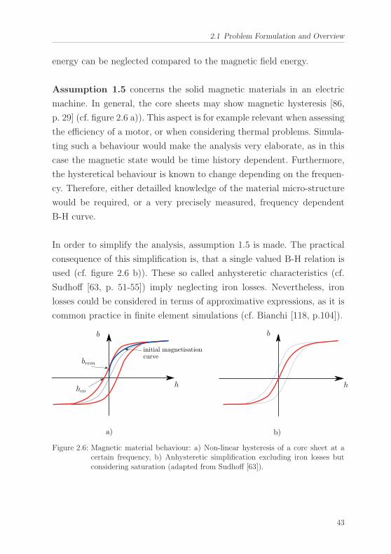
2.1 Problem Formulation and Overview
energy can be neglected compared to the magnetic field energy.
Assumption 1.5 concerns the solid magnetic materials in an electric
machine. In general, the core sheets may show magnetic hysteresis [86,
p. 29] (cf. figure 2.6 a)). This aspect is for example relevant when assessing
the efficiency of a motor, or when considering thermal problems. Simula-
ting such a behaviour would make the analysis very elaborate, as in this
case the magnetic state would be time history dependent. Furthermore,
the hysteretical behaviour is known to change depending on the frequen-
cy. Therefore, either detailled knowledge of the material micro-structure
would be required, or a very precisely measured, frequency dependent
B-H curve.
In order to simplify the analysis, assumption 1.5 is made. The practical
consequence of this simplification is, that a single valued B-H relation is
used (cf. figure 2.6 b)). These so called anhysteretic characteristics (cf.
Sudhoff [63, p. 51-55]) imply neglecting iron losses. Nevertheless, iron
losses could be considered in terms of approximative expressions, as it is
common practice in finite element simulations (cf. Bianchi [118, p.104]).
h
b
brem
hco
initial magnetisationcurve
a)
h
b
b)
Figure 2.6: Magnetic material behaviour: a) Non-linear hysteresis of a core sheet at acertain frequency, b) Anhysteretic simplification excluding iron losses butconsidering saturation (adapted from Sudhoff [63]).
43
2 Model
The consideration of thermal problems is excluded due to assumption
1.7. In many cases, thermal aspects may be very important for electrical
machines. However, since this contribution focuses on the electromecha-
nical coupling thermal effects shall be neglected.
Besides these fundamental conditions, there are individual assumptions
to be made for the different subproblems. As each system part will be
discussed in more detail later, the corresponding assumptions will be dis-
cussed when deriving the governing equations for each subproblem.
The procedure of deriving the system equations for the combined pro-
blem is in a sense a complex task, as the different subproblems require
the application of particular solution techniques and modelling metho-
dologies. Nevertheless, it is possible to cast the whole problem into a
common framework using the Lagrange-Maxwell equations in the
context of analytical dynamics. This common framework is established
in the following section and compared to the classical derivation of the
governing equations using the Newton-Faraday equations. After that,
each subproblem is analysed individually, starting with the mechanical
part, followed by the electrical equations and the magnetic field problem.
As a last section in this chapter, the combined set of differential and al-
gebraic equations are presented and the numerical solution procedure is
outlined.
44
2.2 Electromechanical System Equations
2.2 Electromechanical System Equations
Crandall et al. [114, p. 2] demonstrate the application of both classical
and analytical approaches to derive a set of electromechanical system
equations. As they point out, certainly both classes ultimately lead to
the same governing equations. However, especially analytical approaches
may give additional physical insights to the problem which cannot be
found using classical dynamics. Therefore, both methods are applied and
compared within this section.
2.2.1 The Classical Approach (Newton-Faraday)
Finding the governing equations using a classical approach involves the
following steps [114, p. 300]
• Stating fundamental axioms in terms of Newton’s and Euler’s
equations of motion and Faraday’s law of induction.
• Eliminating dependent variables by fulfilling all kinematical cons-traints and Kirchhoff’s current law.
• Defining the electromechanical coupling in terms of torque, force andflux linkage as a constitutive relation.
After the first two steps, the following structure of equations is obtained
when collecting all individual expressions in matrices (compare Woodson
and Melcher [115, pp. 15–55])
mechanical subsystem:d
dt(Mx) = Fm + Fmag, (2.27a)
electrical subsystem:dλ
dt= ve, (2.27b)
with corresponding initial conditions
x(t = 0) = x0, x(t = 0) = x0 and i(t = 0) = i0.
As there are no capacitive elements in the electrical circuits (assumption
1.4), currents i instead of charges q can be used to describe the electric
45
2 Model
state.
In equation (2.27a) M(x) ∈ Rnm×nm is the mechanical mass and inertia
matrix, Fm(x, x, t) ∈ Rnm comprises all torque and forces expressions of
mechanical origin and Fmag(x, i) ∈ Rnm contains all torques and forces
of magnetical origin.
In equation (2.27b) λ(x, i) ∈ Rne gathers the flux linkages corresponding
to the currents, collected in i ∈ Rne. On the right hand side ve(i, t) ∈ R
ne
are non-inductive voltages (for example resistive voltages, supply voltages
etc.).
The torque and force expressions collected in Fmag and the flux linkage
matrix λ define the electromechanical coupling. Torque and forces are
calculated from the Maxwell stress tensor and flux linkages by sum-
marising the contributions of all ncl coils, through which the associated
currents flow. Thus, the coupling as stated in equations (2.3) and (2.19)
reads
�fmag =
∫SB(��Tmag · �n) dA, �τ (M)
mag =
∫SB�rS × (
��Tmag · �n) dA, (2.28a)
λ =
ncl∑k=1
Nk
∫Smesh,k
�b · �n dA. (2.28b)
And the Maxwell stress tensor becomes
��Tmag = �b⊗ �h− 1
2(�b · �h)��I. (2.29)
How the expressions from the definitions in (2.28a) and (2.28b) enter into
the matrices Fmag and λ depends on the choice of the coordinate system
and is discussed in sections 2.3 and 2.4. The fact that both torque and
force, as well as the flux linkage solely depend on x and i and not on their
time derivatives is a consequence of assumption 1.2. Due to this conditi-
on the quasi stationary solution �b of the magnetic field problem can only
46
2.2 Electromechanical System Equations
depend on the dynamic variables (displacements and currents) directly,
i.e. �b = �b(x, i). This fact can be seen from equations (2.15a): As stated
before, the currents are the only source to the field. Furthermore, when
integrating the equations with respect to a spatial domain, only a mecha-
nical displacement x may deform or shift the integration boundaries and
therefore affect the field solution. Velocities, or other time derivatives are
excluded, as the equations are static.
Therefore, the magnetic field can neihter exert velocitiy proportional ma-
gnetic damping, or gyroscopic forces, nor acceleration proportional forces
in the sense of added mass effects (as it is the case in fluid dynamics,
cf. Brennen [119]). Although often claimed otherwise, electromechanical
energy dissipation is due to induction and resistive dissipation in the
electrical circuits. There is no magnetic damping in the sense of energy
dissipation in the magnetic field. The occuring forces are always positional
in the sense of conservative, or circulatory forces (cf. Merkin [96, p.160]).
The dynamic dependency has a vital influence on the system dynamics
(compare Boy and Hetzler [95]) and should be correctly accounted for.
2.2.2 The Analytical Approach (Lagrange-Maxwell)
When applying an analytical approach, the following steps have to betaken ([114, p. 301 - 302]):
• Chosing a set of kinematically admissible displacements and cur-rents, which identically fulfill the kinematical constraints for boththe mechanical and the electrical subsystem.
• Defining an action functional, such that Newton’s and Euler’s
equations of motion, as well as Faraday’s law of induction are ful-filled, if the action becomes stationary with respect to the solutiontrajectory (for example Hamilton’s principle).
In this second class of problems the electromagnetical coupling is regar-
ded as an integral part of the energy functional. The constitutive relations
47
2 Model
in terms of torque, force and induced voltage are derived from it.
In electromechanical systems, the lagrangian can be expressed by4
L = (T ∗ +W ∗mag)− (V +We), (2.30)
(compare [114, p.302]). Here, T ∗(x, x) is the kinetic co-energy,W ∗mag(x, i)
is the magnetic co-energy and V (x) is the mechanical potential energy.
The electrical energy We can be neglected compared to the magnetic co-
energy as stated in assumption 1.2. This also implies, that none of the
energies depends on the generalised charges q, but only on their derivati-
ves i = q. Therefore, the currents can be used as generalised coordinates
in the following.
Co-energies are defined by Legendre transformations (cf. Crandall et al.
[114, p.13], or appendix A) of the associated energies. The fact that the
Lagrangian is partially defined by co-energies is due to the chosen state
variables x and i. Energy functionals are derived by integrating certain
state equations. In the case of mechanics, the kinetic state equation relates
the momentum p to the velocity v = x, or vice versa5
p = Mv. (2.31)
Depending on whether p, or v is chosen as the independent variable, a
different energy functional is obtained. Thus, the kinetic energy T and
the kinetic co-energy T ∗ are defined by
T =
∫ p
0
v� dp, T ∗ = v�p− T =
∫ v
0
p� dv. (2.32)
In figure 2.7 a), this definition is illustrated for a one-dimensional example.
4The concept of energy and co-energy functionals as state functions and the involved Legendre
transformation appear to be non-standard both in mechanical, as well as in electrical engineering.In Appendix A the most important fundamentals concerning this subject are summarised.
5Although the symbols for linear momentum and translational velocity are used, equation (2.31)also accounts for rotational motions. This is due to the fact, that p and v contain all generalisedcoordinates and M is the generalised mass and inertia matrix.
48
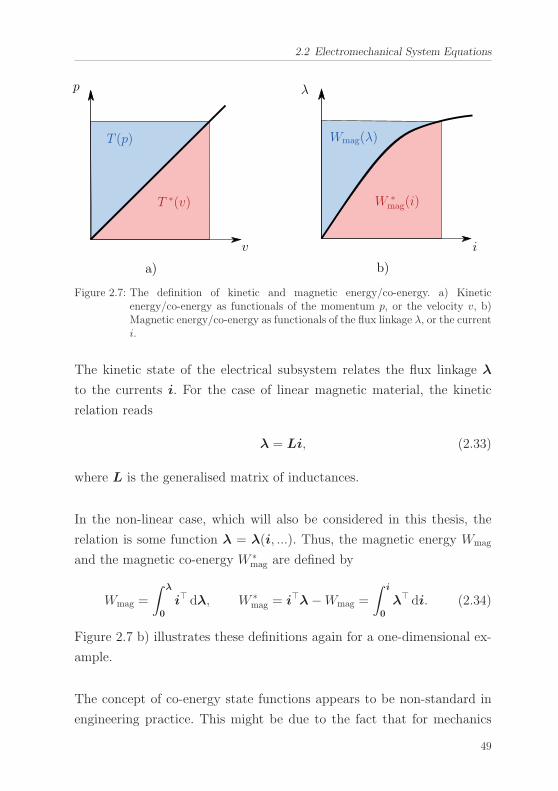
2.2 Electromechanical System Equations
a) b)
p λ
v i
T (p)
T ∗(v)
Wmag(λ)
W ∗mag(i)
Figure 2.7: The definition of kinetic and magnetic energy/co-energy. a) Kineticenergy/co-energy as functionals of the momentum p, or the velocity v, b)Magnetic energy/co-energy as functionals of the flux linkage λ, or the currenti.
The kinetic state of the electrical subsystem relates the flux linkage λ
to the currents i. For the case of linear magnetic material, the kinetic
relation reads
λ = Li, (2.33)
where L is the generalised matrix of inductances.
In the non-linear case, which will also be considered in this thesis, the
relation is some function λ = λ(i, ...). Thus, the magnetic energy Wmag
and the magnetic co-energy W ∗mag are defined by
Wmag =
∫ λ
0
i� dλ, W ∗mag = i�λ−Wmag =
∫ i
0
λ� di. (2.34)
Figure 2.7 b) illustrates these definitions again for a one-dimensional ex-
ample.
The concept of co-energy state functions appears to be non-standard in
engineering practice. This might be due to the fact that for mechanics
49
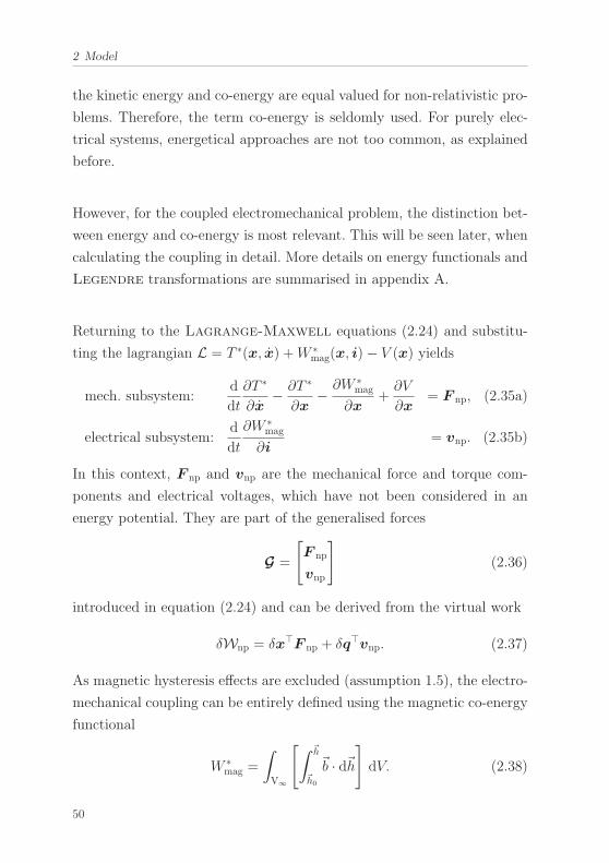
2 Model
the kinetic energy and co-energy are equal valued for non-relativistic pro-
blems. Therefore, the term co-energy is seldomly used. For purely elec-
trical systems, energetical approaches are not too common, as explained
before.
However, for the coupled electromechanical problem, the distinction bet-
ween energy and co-energy is most relevant. This will be seen later, when
calculating the coupling in detail. More details on energy functionals and
Legendre transformations are summarised in appendix A.
Returning to the Lagrange-Maxwell equations (2.24) and substitu-
ting the lagrangian L = T ∗(x, x) +W ∗mag(x, i)− V (x) yields
mech. subsystem:d
dt
∂T ∗
∂x− ∂T ∗
∂x− ∂W ∗
mag
∂x+∂V
∂x= F np, (2.35a)
electrical subsystem:d
dt
∂W ∗mag
∂i= vnp. (2.35b)
In this context, F np and vnp are the mechanical force and torque com-
ponents and electrical voltages, which have not been considered in an
energy potential. They are part of the generalised forces
G =
[F np
vnp
](2.36)
introduced in equation (2.24) and can be derived from the virtual work
δWnp = δx�F np + δq�vnp. (2.37)
As magnetic hysteresis effects are excluded (assumption 1.5), the electro-
mechanical coupling can be entirely defined using the magnetic co-energy
functional
W ∗mag =
∫V∞
[∫ �h
�h0
�b · d�h]dV. (2.38)
50
2.2 Electromechanical System Equations
In this relation V∞ is the whole space and the index 0 defines the state,
where no magnetic field exists. If the magnetic field is known dependin-
ging on the motion and currents (�b = �b(x, i)), the functional can be found
by integration.
Analogously to the derivation of the electromechanical coupling for the
classical approach it can be concluded that due to assumption 1.2, the
magnetic co-energy can only directly depend on the dynamic variables
x and i (W ∗mag = W ∗
mag(x, i)), but not on their time derivatives (as for
example v = x).
2.2.3 Comparing the Classical and Analytical Approaches
Since all kinematical constraints are scleronomous and holonomic (ass-
umption 1.6), the kinetic co-energy will only depend on the system coor-
dinates x and their time derivatives x and has the structure6
T ∗ =1
2x�M(x)x. (2.39)
To compare both classes of approaches, this expression is substituted into
equation (2.35a). If the force and voltage matrices in equations (2.27) are
set according to
Fm = F np − ∂V
∂xand ve = vnp, (2.40)
it can be seen by comparison of equations (2.27) and (2.35), that
Fmag =∂W ∗
mag
∂x
∣∣∣∣i
, λ =∂W ∗
mag
∂i
∣∣∣∣x
, (2.41)
or equivalently
dW ∗mag = dx�Fmag + di�λ . (2.42)
6Assuming scleronomous constraints assures, that there are no prescribed (explicitly time dependent)transport motions. Therefore, the kinetic Energy has no part which is linear, or constant withrespect to x.
51
2 Model
This shows how the system equations (2.27) and (2.35) of both approaches
are related.
In certain situations it is advantageous to calculate the magnetic torques
and forces from the magnetic energy instead of the co-energy. Applying
the Legendre transformation (compare appendix A)
dWmag = d(i�λ)− dW ∗mag = dλ�i− dx�Fmag (2.43)
shows that
i =∂Wmag
∂λ
∣∣∣∣x
, Fmag = −∂Wmag
∂x
∣∣∣∣λ
. (2.44)
The advantage comes into play, when evaluating the gradients: For the
magnetic energy, the flux linkage λ instead of the currents i has to be held
constant in order to evaluate the torques and forces Fmag. The important
point is, that if the flux linkages are held constant, the entire magnetic
field has to be held constant. This allows to focus the analysis to the part
of the magnetic energy in regions, which are deformed due to the motion
x. In the case of an electrical machines, this region is the air-gap. Thus,
the energy in the solid domains does not contribute to the formation of
magnetic forces and torque (compare Ostovic [120, p. 75-81]).
In view of the considerations above, the benefit of comparing classical and
analytical approaches becomes clear. Applying an analytical method, the
energy relations (2.41) and (2.42) are inherently fulfilled and the magne-
tic torque and forces can be calculated both from the magnetic energy,
or co-energy. On the other hand, also when using the classical approach
the energy relations linking both model parts have to be fulfilled. Cer-
tainly, if the field solution �b would be calculated exactly with the classical
equations, the energy relations would be met. However, introducing ap-
proximations, or certain assumptions, they may be violated. Therefore,
it is not self-evident, that the energy relations hold. Notably, this issue
has been discussed in the literature (compare Jordan et al. [19, p. 120-
52
2.2 Electromechanical System Equations
124]). The importance of establishing an energetically consistent coupling
should not be underestimated, as an artificial creation or dissipation of
magnetic energy due to approximation errors may have significant effects
on the dynamic behaviour of the system and thus on the prediction of
vibrations.
As a consequence of relations (2.41) and (2.42), the induced voltage vind
can be found by differentiating the flux linkage as an energy gradient with
respect to time
vind = − d
dt
∂W ∗mag
∂i= −dλ
dt= −∂λ
∂i
di
dt− ∂λ
∂xx. (2.45)
From this relation it can be seen, that there are two parts contributing to
the induced voltage. While the first term is proportional to the time deri-
vative didt of the currents (static induction), the latter one is proportional
to the mechanical velocity x (motion induction). As a conclusion, conside-
ring equations (2.41) and (2.45) shows, that in general the electromagnetic
coupling is mutual: the electrical subsystem affects the mechanical part
via torque and forces and in return the mechanical motion causes induc-
tion into the electric circuits. While this conclusion is quite obvious (and
well known) when discussing the rotational motion in electrical machines,
it might be less apparent when it comes to lateral displacements. Howe-
ver, especially in the latter case, the mutuality of the coupling might be
important when for example self-excited oscillations are to be analysed.
53
2 Model
2.2.4 Qualitative Behaviour of the Coupling
Within this work, both magnetically linear and non-linear material be-
haviours are investigated. However, to get an insight into the qualitative
behaviour of the coupling, a linear constitutive relation for the magne-
tic field shall be assumed for this discourse. For the non-linear material,
analogous considerations are possible.
When assuming a linear constitutive relation, the magnetic co-energy can
be written as
W ∗mag =
1
2i�L(x)i, (2.46)
where L ∈ Rne×ne is the generalised matrix of inductance. Consequently,
the magnetic torque, force and the flux linkage read
Fmag =∂W ∗
mag
∂x=
1
2i�∂L(x)
∂xi and λ =
∂W ∗mag
∂i= L(x)i. (2.47)
Relations (2.47) show, that even if the inductance matrix was linear in x
(which it is not in the general case), the coupling still is inherently non-
linear. This statement can also be extended to systems including non-
linear magnetic behaviour, as the torque and forces, defined in equation
(2.28a) are always non-linear functions of the magnetic flux density. This
conclusion is especially relevant, when investigating the dynamic system
behaviour, as a linear analysis would greatly simplify the problem, but
might not be possible without imposing too strong assumptions. Equati-
ons (2.47) also explain, why the magnetic spring constant introduced by
Fruchtenicht et al. [20] are strongly dependent on the operational condi-
tion. Changing the load or the speed changes the currents and therefore
the magnetic force.
In conclusion, expressing the torque and forces directly in dependence of
the dynamic variables x and i allows for an alternative perspective on
the formation of this part of the coupling.
54
2.2 Electromechanical System Equations
A commonly employed explanation for the creation of torque and forces
is the interaction of different field harmonics in the air gap of the machine
(cf. Seinsch [121, p. 34, 71, 106]). This kind of explanation takes advantage
of the fact, that any field expression in the air gap has to be periodic with
respect to the circumferencial coordinate θ. Under these circumstances,
it can be written in terms of a Fourier series, where
�b = br�er + bt�et and br/t =∞∑
ν=−∞br/t,νe
−jνθ.
Here br/t,ν is the ν-th complex harmonic and j is the imaginary unit.
In this sense, it can be deduced from the classical magnetic torque and
force equations (2.28a) using the Maxwell stress tensor, that magnetic
torque is mainly created by equal field harmonics (order ν) of the radial
component of the flux density br in interaction with the tangential com-
ponent of the magnetic field ht. Analogously, magnetic forces are mainly
caused by adjacent harmonics (ν and ν ± 1) of the radial component of
the flux density br (further details on this are discussed in section 4.1.2).
This explanation precisely shows how the torque and forces depend on the
magnetic field. However, it somehow disguises their dependency on the
dynamic variables x and i. As an alternative to the above interpretation,
relation (2.47) shows, that both torque and forces are caused by a change
of inductance due to the mechanical motion. Here it becomes obvious that,
at least in a magnetically linear case, both torque and forces are quadratic
forms in the current. From this point of view, the analytical approach
shows, that if the matrix of inductance is known as an analytical function,
the torque and forces of magnetic origin can be expressed straight forward
as functions of the dynamic variables. This point and further questions on
the magnetical non-linear behaviour are further adressed in section 2.6.
55
2 Model
2.2.5 Conclusions
To summarise the discussion on the electromechanical system equations
and given the fact that assumptions 1 are considered valid the following
conclusions can be drawn:
Conclusions 1: Electromechanical system equations
1. Based on assumption 1.2, the solution of the magnetic fieldproblem and thus the electromechanical coupling are quasistationary and therefore solely depend on the displacementsx and currents i, but not on their time derivatives.
2. As a consequence, magnetic damping forces, or added mass ef-fects are physically impossible. Electromechanical dissipationis meadiated by induction and takes place in resistive elementsin the electrical circuits. Magnetic forces show either conser-vative, or circulatory behaviour.
3. The electromechanical coupling is mutual. Therefore, it is notpossible to seperate the mechanical from the electrical subsys-tem or vice versa in a general case.
4. The electromechanical coupling stated in terms of torque, forceand flux linkage has to fulfil equations (2.41), or (2.42) to beenergetically consistent.
5. As a consequence of equation (2.28a) and (2.38), it can be con-cluded, that the dependency of the electromechanical couplingon the dynamic variables is inherently non-linear. The ana-lysis shows, why synthetically introduced magnetic stiffnessconstants are strongly load dependent.
56
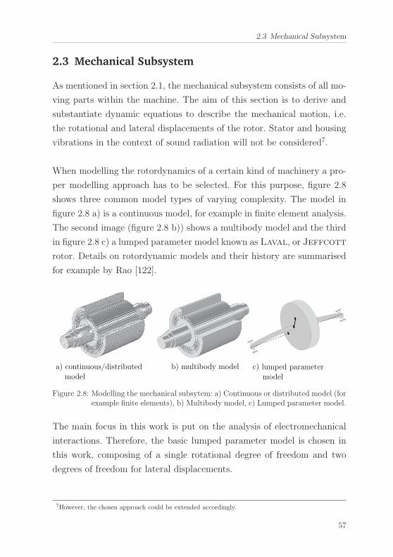
2.3 Mechanical Subsystem
2.3 Mechanical Subsystem
As mentioned in section 2.1, the mechanical subsystem consists of all mo-
ving parts within the machine. The aim of this section is to derive and
substantiate dynamic equations to describe the mechanical motion, i.e.
the rotational and lateral displacements of the rotor. Stator and housing
vibrations in the context of sound radiation will not be considered7.
When modelling the rotordynamics of a certain kind of machinery a pro-
per modelling approach has to be selected. For this purpose, figure 2.8
shows three common model types of varying complexity. The model in
figure 2.8 a) is a continuous model, for example in finite element analysis.
The second image (figure 2.8 b)) shows a multibody model and the third
in figure 2.8 c) a lumped parameter model known as Laval, or Jeffcott
rotor. Details on rotordynamic models and their history are summarised
for example by Rao [122].
a) continuous/distributed
model
b) multibody model c) lumped parameter
model
Figure 2.8: Modelling the mechanical subsytem: a) Continuous or distributed model (forexample finite elements), b) Multibody model, c) Lumped parameter model.
The main focus in this work is put on the analysis of electromechanical
interactions. Therefore, the basic lumped parameter model is chosen in
this work, composing of a single rotational degree of freedom and two
degrees of freedom for lateral displacements.
7However, the chosen approach could be extended accordingly.
57
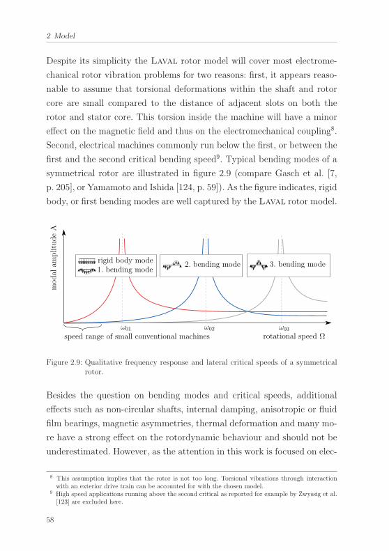
2 Model
Despite its simplicity the Laval rotor model will cover most electrome-
chanical rotor vibration problems for two reasons: first, it appears reaso-
nable to assume that torsional deformations within the shaft and rotor
core are small compared to the distance of adjacent slots on both the
rotor and stator core. This torsion inside the machine will have a minor
effect on the magnetic field and thus on the electromechanical coupling8.
Second, electrical machines commonly run below the first, or between the
first and the second critical bending speed9. Typical bending modes of a
symmetrical rotor are illustrated in figure 2.9 (compare Gasch et al. [7,
p. 205], or Yamamoto and Ishida [124, p. 59]). As the figure indicates, rigid
body, or first bending modes are well captured by the Laval rotor model.
rotational speed Ω
modal
amplitudeA
ω01 ω02 ω03
speed range of small conventional machines
rigid body mode1. bending mode
2. bending mode 3. bending mode
Figure 2.9: Qualitative frequency response and lateral critical speeds of a symmetricalrotor.
Besides the question on bending modes and critical speeds, additional
effects such as non-circular shafts, internal damping, anisotropic or fluid
film bearings, magnetic asymmetries, thermal deformation and many mo-
re have a strong effect on the rotordynamic behaviour and should not be
underestimated. However, as the attention in this work is focused on elec-
8 This assumption implies that the rotor is not too long. Torsional vibrations through interactionwith an exterior drive train can be accounted for with the chosen model.
9 High speed applications running above the second critical as reported for example by Zwyssig et al.[123] are excluded here.
58
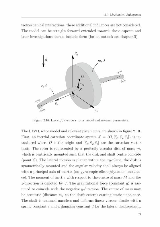
2.3 Mechanical Subsystem
tromechanical interactions, these additional influences are not considered.
The model can be straight forward extended towards these aspects and
later investigations should include them (for an outlook see chapter 5).
c, d
m, J
S
M
O
�ez
�ex
�ey
eM
g
Figure 2.10: Laval/Jeffcott rotor model and relevant parameters.
The Laval rotor model and relevant parameters are shown in figure 2.10.
First, an inertial cartesian coordinate system K = {O, [�ex, �ey, �ez]} is in-
troduced where O is the origin and [�ex, �ey, �ez] are the cartesian vector
basis. The rotor is represented by a perfectly circular disk of mass m,
which is centrically mounted such that the disk and shaft centre coincide
(point S). The lateral motion is planar within the xy-plane, the disk is
symmetrically mounted and the angular velocity shall always be aligned
with a principal axis of inertia (no gyroscopic effects/dynamic unbalan-
ce). The moment of inertia with respect to the centre of mass M and the
z-direction is denoted by J . The gravitational force (constant g) is ass-
umed to coincide with the negative y-direction. The centre of mass may
be eccentric (distance eM to the shaft centre) causing static unbalance.
The shaft is assumed massless and deforms linear viscous elastic with a
spring constant c and a damping constant d for the lateral displacement.
59
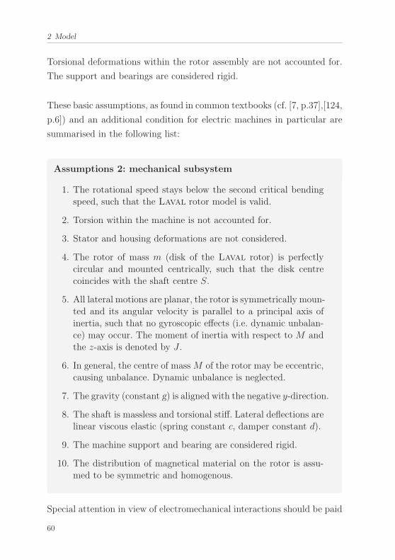
2 Model
Torsional deformations within the rotor assembly are not accounted for.
The support and bearings are considered rigid.
These basic assumptions, as found in common textbooks (cf. [7, p.37],[124,
p.6]) and an additional condition for electric machines in particular are
summarised in the following list:
Assumptions 2: mechanical subsystem
1. The rotational speed stays below the second critical bendingspeed, such that the Laval rotor model is valid.
2. Torsion within the machine is not accounted for.
3. Stator and housing deformations are not considered.
4. The rotor of mass m (disk of the Laval rotor) is perfectlycircular and mounted centrically, such that the disk centrecoincides with the shaft centre S.
5. All lateral motions are planar, the rotor is symmetrically moun-ted and its angular velocity is parallel to a principal axis ofinertia, such that no gyroscopic effects (i.e. dynamic unbalan-ce) may occur. The moment of inertia with respect to M andthe z-axis is denoted by J .
6. In general, the centre of massM of the rotor may be eccentric,causing unbalance. Dynamic unbalance is neglected.
7. The gravity (constant g) is aligned with the negative y-direction.
8. The shaft is massless and torsional stiff. Lateral deflections arelinear viscous elastic (spring constant c, damper constant d).
9. The machine support and bearing are considered rigid.
10. The distribution of magnetical material on the rotor is assu-med to be symmetric and homogenous.
Special attention in view of electromechanical interactions should be paid
60
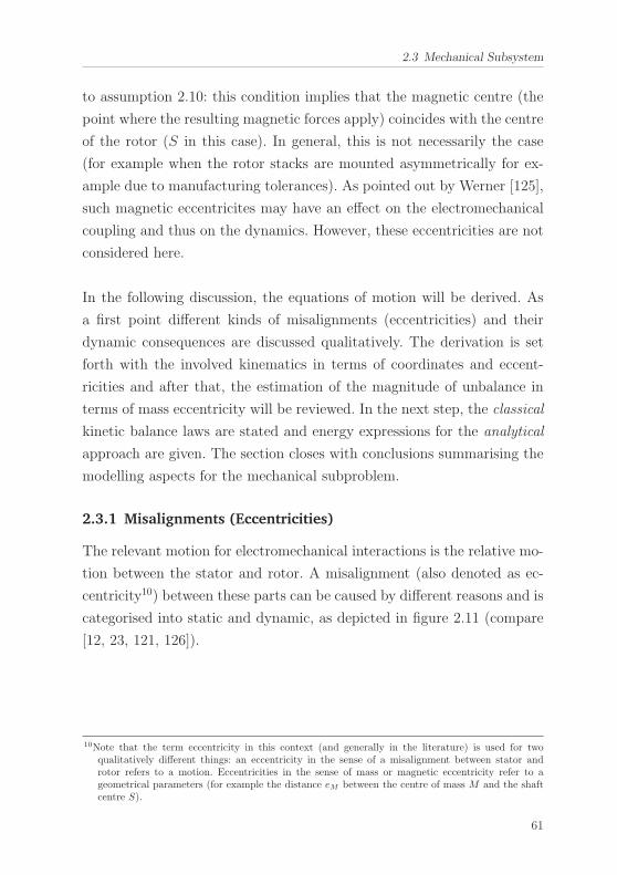
2.3 Mechanical Subsystem
to assumption 2.10: this condition implies that the magnetic centre (the
point where the resulting magnetic forces apply) coincides with the centre
of the rotor (S in this case). In general, this is not necessarily the case
(for example when the rotor stacks are mounted asymmetrically for ex-
ample due to manufacturing tolerances). As pointed out by Werner [125],
such magnetic eccentricites may have an effect on the electromechanical
coupling and thus on the dynamics. However, these eccentricities are not
considered here.
In the following discussion, the equations of motion will be derived. As
a first point different kinds of misalignments (eccentricities) and their
dynamic consequences are discussed qualitatively. The derivation is set
forth with the involved kinematics in terms of coordinates and eccent-
ricities and after that, the estimation of the magnitude of unbalance in
terms of mass eccentricity will be reviewed. In the next step, the classical
kinetic balance laws are stated and energy expressions for the analytical
approach are given. The section closes with conclusions summarising the
modelling aspects for the mechanical subproblem.
2.3.1 Misalignments (Eccentricities)
The relevant motion for electromechanical interactions is the relative mo-
tion between the stator and rotor. A misalignment (also denoted as ec-
centricity10) between these parts can be caused by different reasons and is
categorised into static and dynamic, as depicted in figure 2.11 (compare
[12, 23, 121, 126]).
10Note that the term eccentricity in this context (and generally in the literature) is used for twoqualitatively different things: an eccentricity in the sense of a misalignment between stator androtor refers to a motion. Eccentricities in the sense of mass or magnetic eccentricity refer to ageometrical parameters (for example the distance eM between the centre of mass M and the shaftcentre S).
61
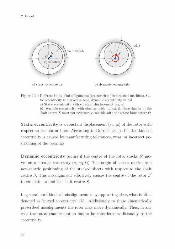
2 Model
e0 = const.
γ0 = const.
a) static eccentricity b) dynamic eccentricity
γd(t)
S ′O
S
S
ed
Figure 2.11: Different kinds of missalignments (eccentricities) in electrical machines. Sta-tic eccentricity is marked in blue, dynamic eccentricity in red.a) Static eccentricity with constant displacement (e0,γ0).b) Dynamic eccentricity with circular orbit (ed,γd(t)). Note that in b) theshaft centre S must not necessarily coincide with the stator bore center O.
Static eccentricity is a constant displacement (e0, γ0) of the rotor with
respect to the stator bore. According to Dorrell [23, p. 14] this kind of
eccentricity is caused by manufacturing tolerances, wear, or incorrect po-
sitioning of the bearings.
Dynamic eccentricity occurs if the centre of the rotor stacks S ′ mo-
ves on a circular trajectory (ed, γd(t)). The origin of such a motion is a
non-centric positioning of the stacked sheets with respect to the shaft
centre S. This misalignment effectively causes the centre of the rotor S ′
to circulate around the shaft centre S.
In general both kinds of misalignments may appear together, what is often
denoted as ’mixed eccentricity’ [75]. Additionaly to these kinematically
prescribed misalignments the rotor may move dynamically. Thus, in any
case the rotordynamic motion has to be considered additionally to the
eccentricity.
62
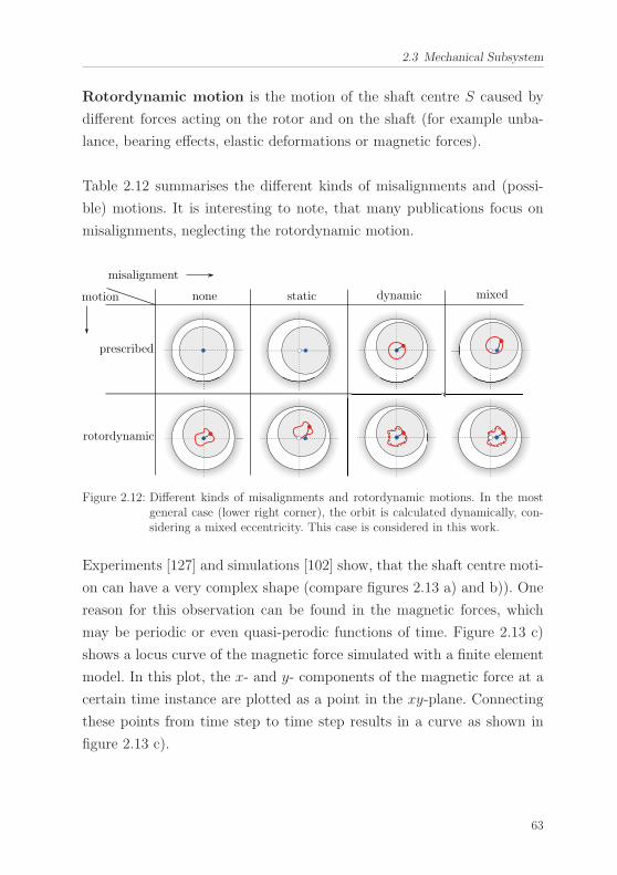
2.3 Mechanical Subsystem
Rotordynamic motion is the motion of the shaft centre S caused by
different forces acting on the rotor and on the shaft (for example unba-
lance, bearing effects, elastic deformations or magnetic forces).
Table 2.12 summarises the different kinds of misalignments and (possi-
ble) motions. It is interesting to note, that many publications focus on
misalignments, neglecting the rotordynamic motion.
none static dynamicmotion
misalignment
prescribed
rotordynamic
mixed
Figure 2.12: Different kinds of misalignments and rotordynamic motions. In the mostgeneral case (lower right corner), the orbit is calculated dynamically, con-sidering a mixed eccentricity. This case is considered in this work.
Experiments [127] and simulations [102] show, that the shaft centre moti-
on can have a very complex shape (compare figures 2.13 a) and b)). One
reason for this observation can be found in the magnetic forces, which
may be periodic or even quasi-perodic functions of time. Figure 2.13 c)
shows a locus curve of the magnetic force simulated with a finite element
model. In this plot, the x- and y- components of the magnetic force at a
certain time instance are plotted as a point in the xy-plane. Connecting
these points from time step to time step results in a curve as shown in
figure 2.13 c).
63
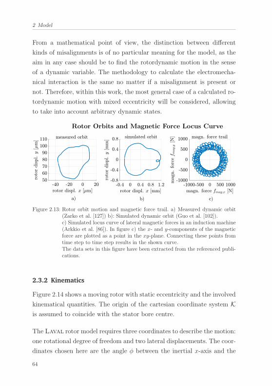
2 Model
From a mathematical point of view, the distinction between different
kinds of misalignments is of no particular meaning for the model, as the
aim in any case should be to find the rotordynamic motion in the sense
of a dynamic variable. The methodology to calculate the electromecha-
nical interaction is the same no matter if a misalignment is present or
not. Therefore, within this work, the most general case of a calculated ro-
tordynamic motion with mixed eccentricity will be considered, allowing
to take into account arbitrary dynamic states.
Rotor Orbits and Magnetic Force Locus Curve
Figure 2.13: Rotor orbit motion and magnetic force trail. a) Measured dynamic orbit(Zarko et al. [127]) b): Simulated dynamic orbit (Guo et al. [102]).c) Simulated locus curve of lateral magnetic forces in an induction machine(Arkkio et al. [86]). In figure c) the x- and y-components of the magneticforce are plotted as a point in the xy-plane. Connecting these points fromtime step to time step results in the shown curve.The data sets in this figure have been extracted from the referenced publi-cations.
2.3.2 Kinematics
Figure 2.14 shows a moving rotor with static eccentricity and the involved
kinematical quantities. The origin of the cartesian coordinate system Kis assumed to coincide with the stator bore centre.
The Laval rotor model requires three coordinates to describe the motion:
one rotational degree of freedom and two lateral displacements. The coor-
dinates chosen here are the angle φ between the inertial x-axis and the
64
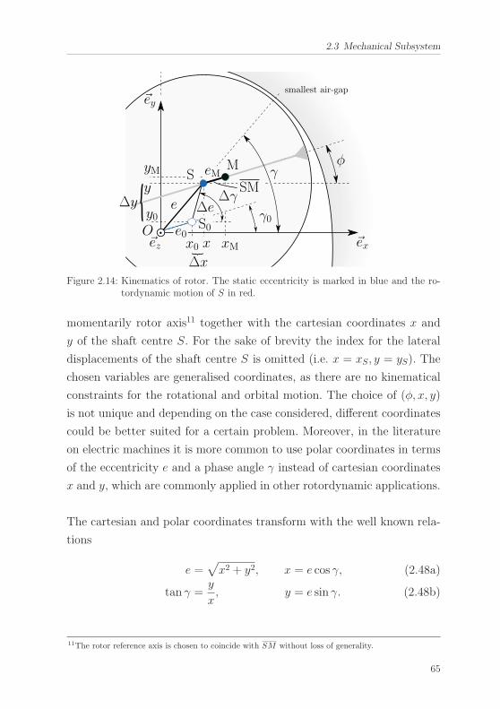
2.3 Mechanical Subsystem
smallest air-gap
�ex
�ey
�ez
MS
S0O
e Δe
e0
eM
x0 x xM
yMy
y0
φγ
γ0
ΔγSM
Δx
Δy
Figure 2.14: Kinematics of rotor. The static eccentricity is marked in blue and the ro-tordynamic motion of S in red.
momentarily rotor axis11 together with the cartesian coordinates x and
y of the shaft centre S. For the sake of brevity the index for the lateral
displacements of the shaft centre S is omitted (i.e. x = xS, y = yS). The
chosen variables are generalised coordinates, as there are no kinematical
constraints for the rotational and orbital motion. The choice of (φ, x, y)
is not unique and depending on the case considered, different coordinates
could be better suited for a certain problem. Moreover, in the literature
on electric machines it is more common to use polar coordinates in terms
of the eccentricity e and a phase angle γ instead of cartesian coordinates
x and y, which are commonly applied in other rotordynamic applications.
The cartesian and polar coordinates transform with the well known rela-
tions
e =√x2 + y2, x = e cos γ, (2.48a)
tan γ =y
x, y = e sin γ. (2.48b)
11The rotor reference axis is chosen to coincide with SM without loss of generality.
65
2 Model
The resulting shaft eccentricity in terms of (e, γ) is related to the static
eccentricity (e0, γ0) and rotordynamic motion (Δe,Δγ) by
e =√e20 + 2e0Δe cos(γ0 −Δγ) + Δe2, (2.49a)
tan γ =e0 sin γ0 +Δe sinΔγ
e0 cos γ0 +Δe cosΔγ, (2.49b)
what can be seen, when substituting x = x0 + Δx and y = y0 + Δy in
equations (2.48) and using polar coordinates.
With this information the position of the geometric rotor centre S ′, wherethe magnetic forces apply, is determined by
x′ = x+ ed cos γd(t), (2.50a)
y′ = y + ed sin γd(t). (2.50b)
According to assumption 2.6 the centre of mass M is assumed to be
eccentric with respect to the geometrical centre S, causing unbalance.
The coordinates of M are related to those of S by
xM = x+ eM cosφ, (2.51a)
yM = y + eM sinφ, (2.51b)
where the mass eccentricity eM is a geometrical parameter. When simu-
lating the rotordynamics of an electric machine, this parameter takes a
vital role, as it defines the magnitude of the unbalance, which is a major
cause for lateral rotor vibrations.
Estimation of the mass eccentricity
The industry norm ISO 21940 [128] defines how to assess the balance
quality of a rotating machine by a balancing quality grade G. In electrical
machines, it is commonly required to range between G = 1, ... , 3mms . With
this definition, the maximum allowed mass eccentrity eM,max for a certain
66
2.3 Mechanical Subsystem
balance class G can be calculated by
eM,max =G
1000Ωr, (2.52)
where Ωr is the rated angular velocity. This maximum value will be used
in all following considerations (eM := eM,max), providing an upper bound
for the unbalance. The effect of improving the balance quality will also
be discussed. As an example the mass eccentricity in a machine with
balance quality grade G = 1mms and a rated speed of 3000 rpm would be
eM,max ≈ 0.019 mm.
2.3.3 Kinetics
Derived from Newton’s and Euler’s laws of motion and considering
the free body diagram in figure 2.15, the equations of motion read
mx+ dx+ c(x− x0) = meG( φ sinφ+ φ2 cosφ) + fmag,x, (2.53a)
my + dy + c(y − y0) = meG(−φ cosφ+ φ2 sinφ)−mg+ fmag,y, (2.53b)
Jφ = −τL + τmag (2.53c)
+ eG(−c(x− x0)− dx) sinφ− fmag,x(ed sin γd − eM sinφ)
− eG(−c(y − y0)− dy) cosφ− fmag,y(eM cosφ− ed cos γd).
Expressions for the magnetic force components fmag,x, fmag,y and the ma-
getic torque τmag are given in section 2.6. Note that the additional torque
stemming from the magnetic force components is due to the fact that the
magnetic forces apply at the geometric rotor centre S ′, while the torque
balance has been stated with respect to the centre of mass M .
The kinetic co-energy for the Lagrange-Maxwell equations can be
calculated by
T ∗ =1
2m (�vM · �vM) +
1
2Jφ. (2.54)
67
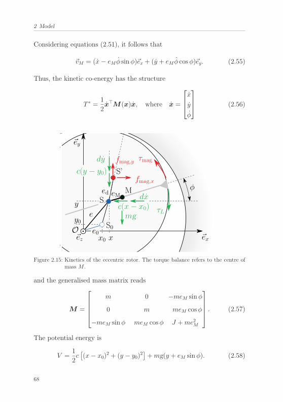
2 Model
Considering equations (2.51), it follows that
�vM = (x− eM φ sinφ)�ex + (y + eM φ cosφ)�ey. (2.55)
Thus, the kinetic co-energy has the structure
T ∗ =1
2x�M(x)x, where x =
⎡⎢⎣xyφ
⎤⎥⎦ (2.56)
�ex
�ey
�ez
S
S0Oe
eM
x0 x
y
y0
φ
c(y − y0)
dy
c(x− x0)dx
τmag
τLmg
M
fmag,y
fmag,x
ed
S’
e0
Figure 2.15: Kinetics of the eccentric rotor. The torque balance refers to the centre ofmass M .
and the generalised mass matrix reads
M =
⎡⎢⎢⎢⎣
m 0 −meM sinφ
0 m meM cosφ
−meM sinφ meM cosφ J +me2M
⎤⎥⎥⎥⎦ . (2.57)
The potential energy is
V =1
2c[(x− x0)
2 + (y − y0)2]+mg(y + eM sinφ). (2.58)
68
2.3 Mechanical Subsystem
The relation for the magnetic co-energy will be given in section 2.5. The
matrix of non-potential mechanical forces
F np =
⎡⎢⎣−dx−dy−τL
⎤⎥⎦ . (2.59)
Substituting equations (2.56)-(2.59) in (2.35a) leads to exactly the sa-
me equations of motion (relations (2.53)) as when using Newton’s and
Euler’s laws.
69
2 Model
2.3.4 Conclusions
To end this section and provided that assumptions 2 are valid the follo-
wing conclusions can be drawn:
Conclusions 2: Mechanical Equations of Motion
1. The chosen Laval/Jeffcott rotor model can be applied,whenever the inner torsion of the machine can be neglectedand the machine runs below the second critical bending speed.
2. The analysis in this work is aiming at the basic electromecha-nical interaction: For the sake of clarity additional rotordyna-mic effects are not considered here. However, they could bestraight forward added to the proposed model.
3. There may be different kinds of misalignments (eccentricities)in an electric machine: static eccentricities with a given con-stant displacement and dynamic eccentricities involving a cir-cular orbit. The chosen modeling approach covers both typesof eccentricities in the context of rotordynamics and thus al-lows for the consideration of arbitrary kinematic states.
4. The mass eccentricity of the rotor is estimated using the ba-lancing quality grade as defined in ISO-21940.
5. The equations of motion for the three degrees of freedom interms of rotation angle and displacement of the shaft centrehave been derived with the classical approach. Moreover, thekinetic co-energy and the potential energy have been statedfor the analytical approach.
70
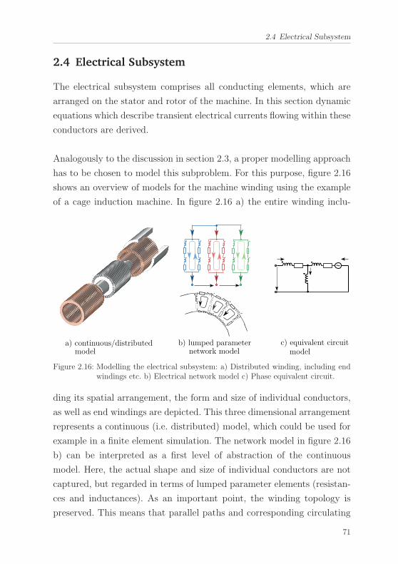
2.4 Electrical Subsystem
2.4 Electrical Subsystem
The electrical subsystem comprises all conducting elements, which are
arranged on the stator and rotor of the machine. In this section dynamic
equations which describe transient electrical currents flowing within these
conductors are derived.
Analogously to the discussion in section 2.3, a proper modelling approach
has to be chosen to model this subproblem. For this purpose, figure 2.16
shows an overview of models for the machine winding using the example
of a cage induction machine. In figure 2.16 a) the entire winding inclu-
a) continuous/distributed b) lumped parameter c) equivalent circuitmodel network model model
Figure 2.16: Modelling the electrical subsystem: a) Distributed winding, including endwindings etc. b) Electrical network model c) Phase equivalent circuit.
ding its spatial arrangement, the form and size of individual conductors,
as well as end windings are depicted. This three dimensional arrangement
represents a continuous (i.e. distributed) model, which could be used for
example in a finite element simulation. The network model in figure 2.16
b) can be interpreted as a first level of abstraction of the continuous
model. Here, the actual shape and size of individual conductors are not
captured, but regarded in terms of lumped parameter elements (resistan-
ces and inductances). As an important point, the winding topology is
preserved. This means that parallel paths and corresponding circulating
71
2 Model
currents are considered. In the last model (figure 2.16 c)), the winding to-
pology is simplified to a single equivalent circuit. The main requirements
for this abstraction level are symmetrical phases and system properties.
Parallel paths cannot be regarded in such an approach. This methodology
and the well known space vector notation can be found in most textbooks
(cf. Binder [12, p. 981 ff.]) and are applied to many electric machine pro-
blems. As a standard tool, it offers a good reference for more complex
models (see also appendix D for more details).
For the modelling of electromechanical interactions, it turned out in sec-
tion 1.1, that irregular magnetic torque and lateral forces are mainly cau-
sed by electromagnetic and electromechanical asymmetries. Their sources
are misalignments like eccentricities, or unequal geometrical or material
distributions and their effects are non-symmetrical phase currents and
circulating currents in parallel paths. It appears to be of decisive import-
ance to regard the actual network topology of a certain winding. In view
of this background and the intention to provide for the least modelling
complexity, while capturing the essential effects, an electric network mo-
del, according to figure 2.16 b) is chosen in this work.
The derivation of electrical network equations presumes further assump-
tions, summarised as follows:
Assumptions 3: electrical subsystem
1. The originally distributed form of the winding is reduced toan electrical network of constant resistances and non-linearinductances.
2. The flux linkage for the inductances in the main part of themachine is calculated from the magnetic field (compare section2.5).
72
2.4 Electrical Subsystem
3. The end windings are regarded as constant resistances andinductances.
4. Leakage effects are accounted for in terms of constant induc-tances.
5. Thermal effects are neglected.
6. Both the skin and the proximity effect are neglected.
These assumptions are rather common when analysing vibration problems
using network models (compare for example Toliyat et al. [33]). However,
assumption 3.6 (neglection of the skin and proximity effect) will not hold
for short time transient, or high frequency processes. For considerations
in future studies the model should be extended to account for these effects.
Within this work, generalised mesh analysis in the context of analyti-
cal dynamics is introduced to state the electrical network equations. The
idea behind this approach is based on so called generalised current coordi-
nates12, which identically fulfill Kirchhoff’s current law. The common
mesh equations, known from fundamental circuit analysis, are transfor-
med to form so called ’generalised meshes’.
In the following, the concept will be explained step by step. To this end,
first generalised currents are introduced, followed by the derivation gene-
ralised mesh equations. Subsequently, the equivalence between generalised
mesh analysis (analytical dynamics) and the common nodal analysis (clas-
sical dynamics) is proven. At the end of the section, phase connections
(star and delta) are shortly adressed. The derivation will be accompanied
by a minimal example of a simple RL-network. The more elaborate to-
pologies (for example a three phase winding with parallel branches, or a
rotor cage) are summarised in appendix D.
12Generalised coordinates, as introduced in section 2.2.2 are a minimal set of variables, uniquely des-cribing the system state. While in mechanics, these coordinates identically fulfil the kinematic cons-traints, in electric networks, this identical fulfilment concerns Kirchhoff’s current law (cf. Neımarkand Fufaev [113, p.3-7]).
73
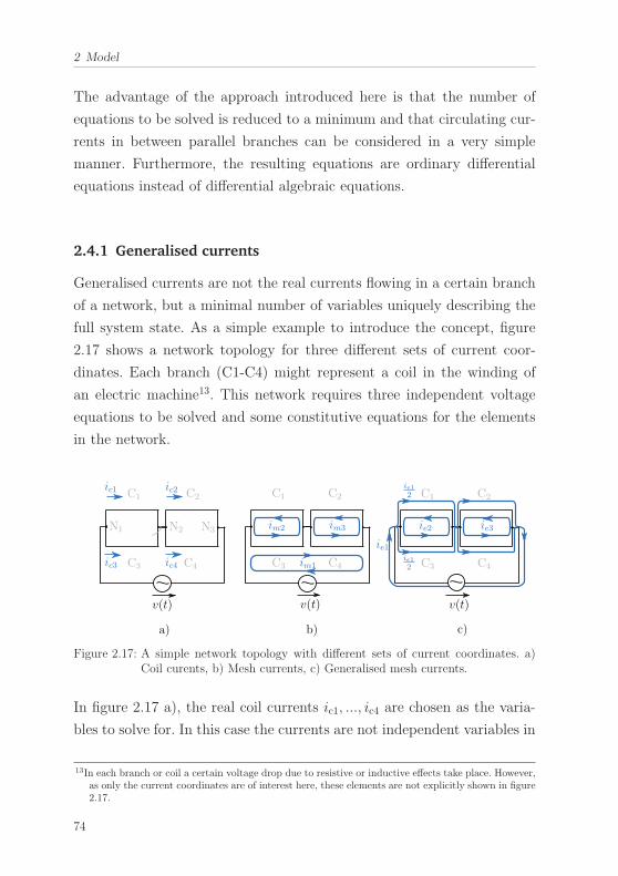
2 Model
The advantage of the approach introduced here is that the number of
equations to be solved is reduced to a minimum and that circulating cur-
rents in between parallel branches can be considered in a very simple
manner. Furthermore, the resulting equations are ordinary differential
equations instead of differential algebraic equations.
2.4.1 Generalised currents
Generalised currents are not the real currents flowing in a certain branch
of a network, but a minimal number of variables uniquely describing the
full system state. As a simple example to introduce the concept, figure
2.17 shows a network topology for three different sets of current coor-
dinates. Each branch (C1-C4) might represent a coil in the winding of
an electric machine13. This network requires three independent voltage
equations to be solved and some constitutive equations for the elements
in the network.
a) b) c)
v(t) v(t) v(t)
C1 C2
C3 C4
ic1 ic2
ic3 ic4
C1 C2
C3 C4
C1 C2
C3 C4
im2 im3 ie2 ie3
im1
ie1ie12
ie12
N1 N3N2
Figure 2.17: A simple network topology with different sets of current coordinates. a)Coil curents, b) Mesh currents, c) Generalised mesh currents.
In figure 2.17 a), the real coil currents ic1, ..., ic4 are chosen as the varia-
bles to solve for. In this case the currents are not independent variables in
13In each branch or coil a certain voltage drop due to resistive or inductive effects take place. However,as only the current coordinates are of interest here, these elements are not explicitly shown in figure2.17.
74
2.4 Electrical Subsystem
the sense of Lagrangian mechanics, as they do not identically fulfill all
node equations14. Thus, for this choice of variables, there are three mesh
equations and one node equation to be solved.
A second set of currents is shown in figure 2.17 b). Here, mesh currents
im1, im2 and im3 are chosen. In contrast to the coil currents, these variables
are generalised coordinates, as all node equations are fulfilled identically.
Thus, for this set of variables, there are only three mesh equations to be
solved. The coil currents can be calculated from the mesh currents by⎡⎢⎢⎢⎢⎣ic1
ic2
ic3
ic4
⎤⎥⎥⎥⎥⎦
︸ ︷︷ ︸ic
=
⎡⎢⎢⎢⎢⎣
0 −1 0
0 0 −1
1 1 0
1 0 1
⎤⎥⎥⎥⎥⎦
︸ ︷︷ ︸T c,m
⎡⎢⎣im1
im2
im3
⎤⎥⎦
︸ ︷︷ ︸im
⇒ ic = T c,mim. (2.60)
The choice of current variables in figure 2.17 b) is somewhat arbitrary and
certainly not unique. In electric machines, a particular choice of coordi-
nates may simplify the analysis considerably. It will be introduced and
explained in the following.
Basically, the electrical part of an electric machine consists of several
RL-networks. In this sense, the example in figure 2.17 could represent
one phase of a three phase winding in the stator of the machine. When
analysing the currents under certain operation conditions, in many cases
only the phase currents are considered. However, if there is some asym-
metry in the system, for example due to eccentricity, equalising currents
in between parallel branches of the winding may occur. From this point
of view, it would make sense to describe the system dynamics in terms of
phase currents representing the symmetrical system state and equalising
currents, accounting for asymmetries.
14They require the additional condition ic1 + ic3 = ic2 + ic4, what can be seen either from nodes N1
and N3, or directly from node N2.
75
2 Model
The set of current coordinates in figure 2.17 c) has been taylored in ex-
actly this sense. While the phase current ie1 equally splits to both parallel
branches, the equalising currents ie2 and ie3 account for differences bet-
ween them. The coil currents can be calculated from these generalised
coordinates by⎡⎢⎢⎢⎢⎣ic1
ic2
ic3
ic4
⎤⎥⎥⎥⎥⎦
︸ ︷︷ ︸ic
=
⎡⎢⎢⎢⎢⎣
12 −1 012 0 −112 1 012 0 1
⎤⎥⎥⎥⎥⎦
︸ ︷︷ ︸T c,e
⎡⎢⎣ie1ie2ie3
⎤⎥⎦
︸ ︷︷ ︸ie
⇒ ic = T c,eie. (2.61)
Having defined the variables to solve for, the next question to answer is
how to derive proper mesh equations in order to determine the currents
as dynamic variables.
2.4.2 Generalised mesh equations
Stating the electrical equations in terms of generalised meshes, the follo-wing steps have to be taken:
1. Defining the coil as a basic element of the winding.
2. Connecting coils to form meshes within an electrical network.
3. Combining ordinary meshes to form generalised meshes.
As before, the minimal example depicted in figure 2.17 will be chosen to
illustrate the basic concept. The more complex network topologies are
summarised in appendix D.
1. Defining the coil as a basic element of a winding
According to Muller et al. [13, p. 3], the elementary part of each winding
is a coil. As illustrated in figure 2.18, a coil having n turns consists of
some terminals, two coil sides and an end winding, connecting the sides.
76
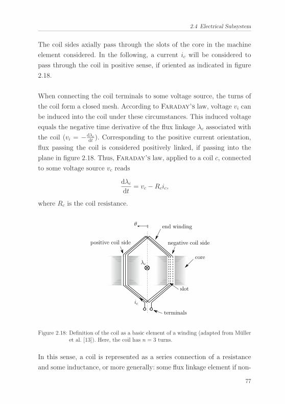
2.4 Electrical Subsystem
The coil sides axially pass through the slots of the core in the machine
element considered. In the following, a current ic will be considered to
pass through the coil in positive sense, if oriented as indicated in figure
2.18.
When connecting the coil terminals to some voltage source, the turns of
the coil form a closed mesh. According to Faraday’s law, voltage vi can
be induced into the coil under these circumstances. This induced voltage
equals the negative time derivative of the flux linkage λc associated with
the coil (vi = −dλcdt ). Corresponding to the positive current orientation,
flux passing the coil is considered positively linked, if passing into the
plane in figure 2.18. Thus, Faraday’s law, applied to a coil c, connected
to some voltage source vc reads
dλcdt
= vc −Rcic,
where Rc is the coil resistance.
end winding
terminals
θ
core
slot
positive coil side negative coil side
ic
λc
Figure 2.18: Definition of the coil as a basic element of a winding (adapted from Mulleret al. [13]). Here, the coil has n = 3 turns.
In this sense, a coil is represented as a series connection of a resistance
and some inductance, or more generally: some flux linkage element if non-
77
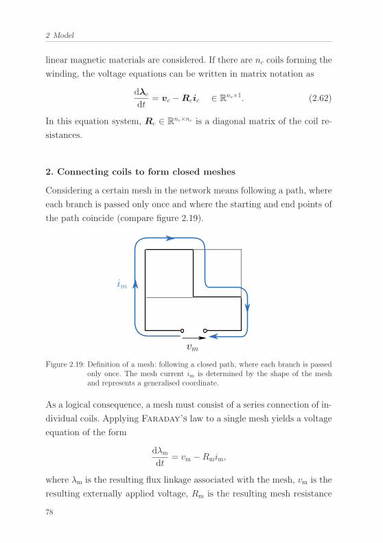
2 Model
linear magnetic materials are considered. If there are nc coils forming the
winding, the voltage equations can be written in matrix notation as
dλc
dt= vc −Rcic ∈ R
nc×1. (2.62)
In this equation system, Rc ∈ Rnc×nc is a diagonal matrix of the coil re-
sistances.
2. Connecting coils to form closed meshes
Considering a certain mesh in the network means following a path, where
each branch is passed only once and where the starting and end points of
the path coincide (compare figure 2.19).
vm
im
Figure 2.19: Definition of a mesh: following a closed path, where each branch is passedonly once. The mesh current im is determined by the shape of the meshand represents a generalised coordinate.
As a logical consequence, a mesh must consist of a series connection of in-
dividual coils. Applying Faraday’s law to a single mesh yields a voltage
equation of the form
dλmdt
= vm −Rmim,
where λm is the resulting flux linkage associated with the mesh, vm is the
resulting externally applied voltage, Rm is the resulting mesh resistance
78
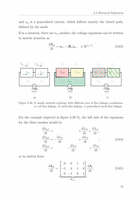
2.4 Electrical Subsystem
and im is a generalised current, which follows exactly the closed path,
defined by the mesh.
If in a network, there are nm meshes, the voltage equations can be written
in matrix notation as
dλm
dt= vm −Rmim ∈ R
nm×1. (2.63)
a) b) c)
v(t) v(t) v(t)
C1 C2
C3 C4
λc1 λc2
λc3 λc4
C1 C2
C3 C4
C1 C2
C3 C4
λm2 λm3 λe2 λe3
λm1
λe12
λe12
Figure 2.20: A simple network topology with different sets of flux linkage coordinates.a) coil flux linkage, b) mesh flux linkage, c) generalised mesh flux linkage.
For the example depicted in figure 2.20 b), the left side of the equations
for the three meshes would be
dλm1
dt= +
dλc3dt
+dλc4dt
,
dλm2
dt= −dλc1
dt+
dλc3dt
, (2.64)
dλm3
dt= −dλc2
dt+
dλc4dt
,
or in matrix form
dλm
dt=
⎡⎢⎣ 0 0 1 1
−1 0 1 0
0 −1 0 1
⎤⎥⎦
︸ ︷︷ ︸Tm,c
dλc
dt. (2.65)
79
2 Model
The mesh and the coil flux linkages are related by
λm = Tm,c λc,
where for the example above Tm,c = T�c,m holds, as it can be seen when
comparing equations (2.60) and (2.65). This relation holds for all genera-
lised current and flux linkage coordinates, whereby proof will be given in
section 2.4.3.
Returning to equations (2.63), the right hand side can also be given ex-
plicitly for the example:
vm −Rmim =
⎡⎢⎣v(t)0
0
⎤⎥⎦
︸ ︷︷ ︸vm
−
⎡⎢⎣ 0 0 1 1
−1 0 1 0
0 −1 0 1
⎤⎥⎦
︸ ︷︷ ︸Tm,c
⎡⎢⎢⎢⎢⎣Rc1 0 0 0
0 Rc2 0 0
0 0 Rc3 0
0 0 0 Rc4
⎤⎥⎥⎥⎥⎦
︸ ︷︷ ︸Rc
⎡⎢⎢⎢⎢⎣ic1
ic2
ic3
ic4
⎤⎥⎥⎥⎥⎦
︸ ︷︷ ︸ic
.
When defining
⎡⎢⎣v(t)0
0
⎤⎥⎦
︸ ︷︷ ︸vm
=
⎡⎢⎣ 0 0 1 1
−1 0 1 0
0 −1 0 1
⎤⎥⎦
︸ ︷︷ ︸Tm,c
⎡⎢⎢⎢⎢⎣v(t)2v(t)2v(t)2v(t)2
⎤⎥⎥⎥⎥⎦
︸ ︷︷ ︸vc
,
it becomes apparent, that in this example, the mesh voltage equations
(2.63) can be derived from the coil voltage equations (2.62) by multiplying
from the left with Tm,c. As before, this statement holds for all meshes,
what will be shown in section 2.4.3.
80
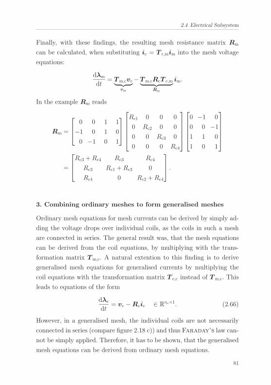
2.4 Electrical Subsystem
Finally, with these findings, the resulting mesh resistance matrix Rm
can be calculated, when substituting ic = T c,mim into the mesh voltage
equations:
dλm
dt= Tm,cvc︸ ︷︷ ︸
vm
−Tm,cRcT c,m︸ ︷︷ ︸Rm
im.
In the example Rm reads
Rm =
⎡⎢⎣ 0 0 1 1
−1 0 1 0
0 −1 0 1
⎤⎥⎦⎡⎢⎢⎢⎢⎣Rc1 0 0 0
0 Rc2 0 0
0 0 Rc3 0
0 0 0 Rc4
⎤⎥⎥⎥⎥⎦
⎡⎢⎢⎢⎢⎣0 −1 0
0 0 −1
1 1 0
1 0 1
⎤⎥⎥⎥⎥⎦
=
⎡⎢⎣Rc3 +Rc4 Rc3 Rc4
Rc3 Rc1 +Rc3 0
Rc4 0 Rc2 +Rc4
⎤⎥⎦ .
3. Combining ordinary meshes to form generalised meshes
Ordinary mesh equations for mesh currents can be derived by simply ad-
ding the voltage drops over individual coils, as the coils in such a mesh
are connected in series. The general result was, that the mesh equations
can be derived from the coil equations, by multiplying with the trans-
formation matrix Tm,c. A natural extention to this finding is to derive
generalised mesh equations for generalised currents by multiplying the
coil equations with the transformation matrix T e,c instead of Tm,c. This
leads to equations of the form
dλe
dt= ve −Reie ∈ R
ne×1. (2.66)
However, in a generalised mesh, the individual coils are not necessarily
connected in series (compare figure 2.18 c)) and thus Faraday’s law can-
not be simply applied. Therefore, it has to be shown, that the generalised
mesh equations can be derived from ordinary mesh equations.
81
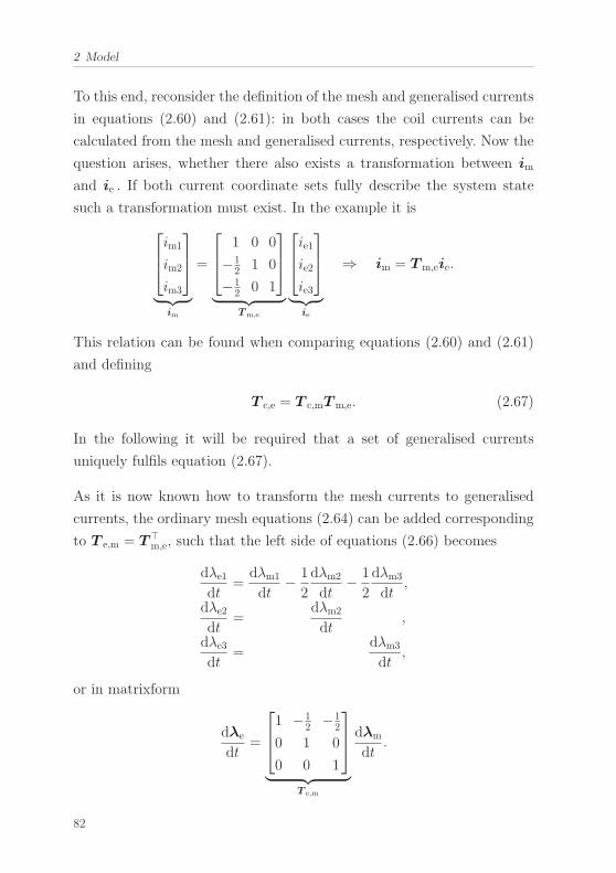
2 Model
To this end, reconsider the definition of the mesh and generalised currents
in equations (2.60) and (2.61): in both cases the coil currents can be
calculated from the mesh and generalised currents, respectively. Now the
question arises, whether there also exists a transformation between im
and ie . If both current coordinate sets fully describe the system state
such a transformation must exist. In the example it is⎡⎢⎣im1
im2
im3
⎤⎥⎦
︸ ︷︷ ︸im
=
⎡⎢⎣ 1 0 0
−12 1 0
−12 0 1
⎤⎥⎦
︸ ︷︷ ︸Tm,e
⎡⎢⎣ie1ie2ie3
⎤⎥⎦
︸ ︷︷ ︸ie
⇒ im = Tm,eie.
This relation can be found when comparing equations (2.60) and (2.61)
and defining
T c,e = T c,mTm,e. (2.67)
In the following it will be required that a set of generalised currents
uniquely fulfils equation (2.67).
As it is now known how to transform the mesh currents to generalised
currents, the ordinary mesh equations (2.64) can be added corresponding
to T e,m = T�m,e, such that the left side of equations (2.66) becomes
dλe1dt
=dλm1
dt− 1
2
dλm2
dt− 1
2
dλm3
dt,
dλe2dt
=dλm2
dt,
dλe3dt
=dλm3
dt,
or in matrixform
dλe
dt=
⎡⎢⎣1 −1
2 −12
0 1 0
0 0 1
⎤⎥⎦
︸ ︷︷ ︸T e,m
dλm
dt.
82
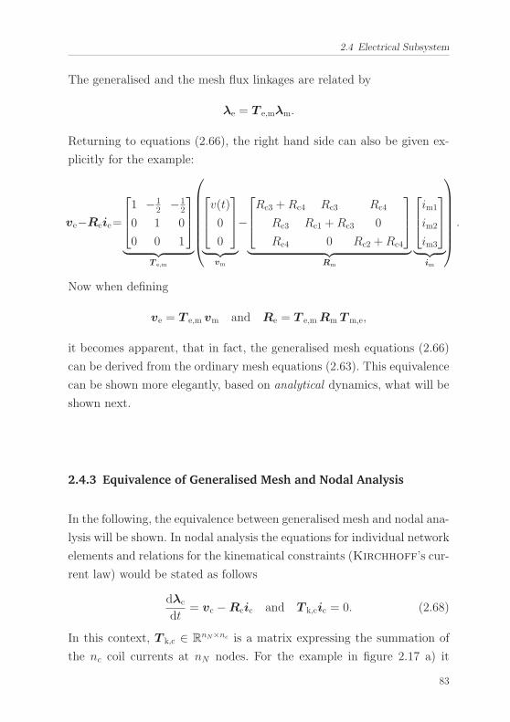
2.4 Electrical Subsystem
The generalised and the mesh flux linkages are related by
λe = T e,mλm.
Returning to equations (2.66), the right hand side can also be given ex-
plicitly for the example:
ve−Reie=
⎡⎢⎣1 −1
2 −12
0 1 0
0 0 1
⎤⎥⎦
︸ ︷︷ ︸T e,m
⎛⎜⎜⎜⎜⎜⎜⎝⎡⎢⎣v(t)0
0
⎤⎥⎦
︸ ︷︷ ︸vm
−
⎡⎢⎣Rc3 +Rc4 Rc3 Rc4
Rc3 Rc1 +Rc3 0
Rc4 0 Rc2 +Rc4
⎤⎥⎦
︸ ︷︷ ︸Rm
⎡⎢⎣im1
im2
im3
⎤⎥⎦
︸ ︷︷ ︸im
⎞⎟⎟⎟⎟⎟⎟⎠ .
Now when defining
ve = T e,m vm and Re = T e,mRm Tm,e,
it becomes apparent, that in fact, the generalised mesh equations (2.66)
can be derived from the ordinary mesh equations (2.63). This equivalence
can be shown more elegantly, based on analytical dynamics, what will be
shown next.
2.4.3 Equivalence of Generalised Mesh and Nodal Analysis
In the following, the equivalence between generalised mesh and nodal ana-
lysis will be shown. In nodal analysis the equations for individual network
elements and relations for the kinematical constraints (Kirchhoff’s cur-
rent law) would be stated as follows
dλc
dt= vc −Rcic and T k,cic = 0. (2.68)
In this context, T k,c ∈ RnN×nc is a matrix expressing the summation of
the nc coil currents at nN nodes. For the example in figure 2.17 a) it
83
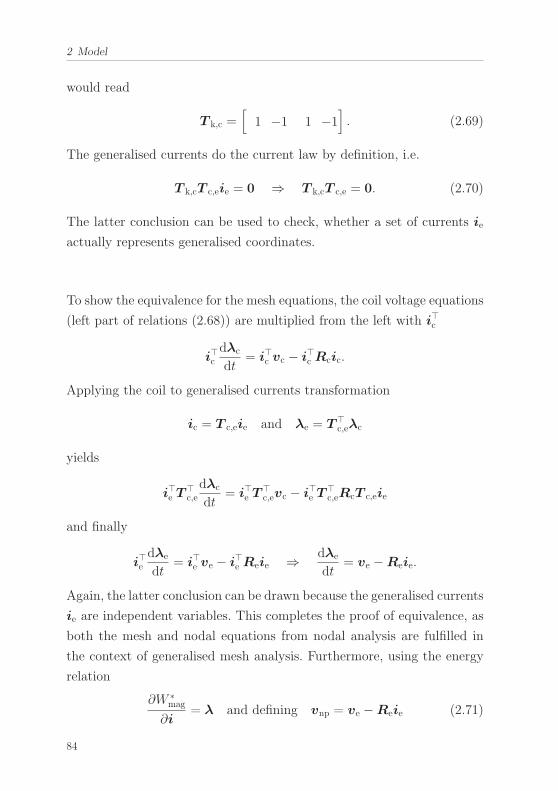
2 Model
would read
T k,c =[
1 −1 1 −1]. (2.69)
The generalised currents do the current law by definition, i.e.
T k,cT c,eie = 0 ⇒ T k,cT c,e = 0. (2.70)
The latter conclusion can be used to check, whether a set of currents ie
actually represents generalised coordinates.
To show the equivalence for the mesh equations, the coil voltage equations
(left part of relations (2.68)) are multiplied from the left with i�c
i�cdλc
dt= i�c vc − i�c Rcic.
Applying the coil to generalised currents transformation
ic = T c,eie and λe = T�c,eλc
yields
i�e T�c,e
dλc
dt= i�e T
�c,evc − i�e T
�c,eRcT c,eie
and finally
i�edλe
dt= i�e ve − i�e Reie ⇒ dλe
dt= ve −Reie.
Again, the latter conclusion can be drawn because the generalised currents
ie are independent variables. This completes the proof of equivalence, as
both the mesh and nodal equations from nodal analysis are fulfilled in
the context of generalised mesh analysis. Furthermore, using the energy
relation
∂W ∗mag
∂i= λ and defining vnp = ve −Reie (2.71)
84
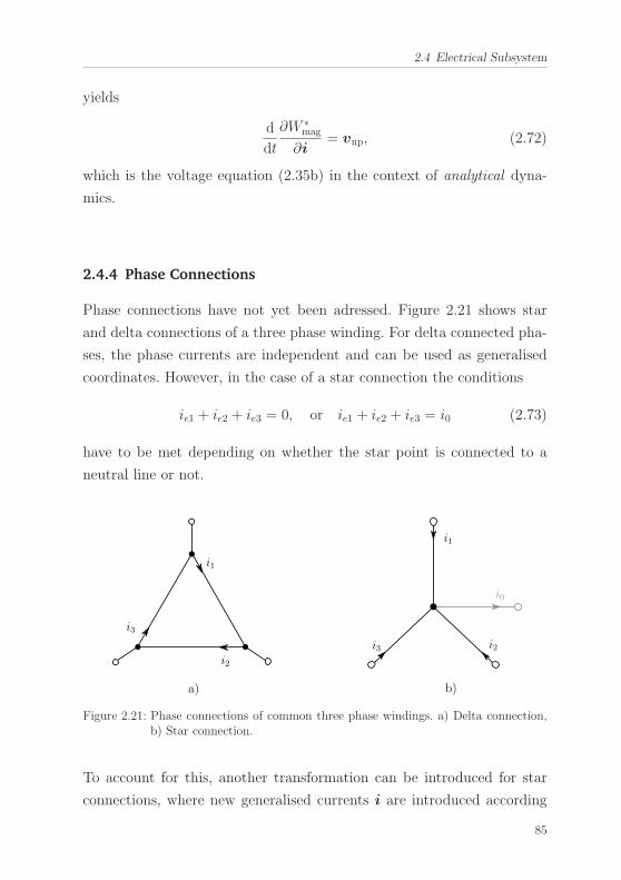
2.4 Electrical Subsystem
yields
d
dt
∂W ∗mag
∂i= vnp, (2.72)
which is the voltage equation (2.35b) in the context of analytical dyna-
mics.
2.4.4 Phase Connections
Phase connections have not yet been adressed. Figure 2.21 shows star
and delta connections of a three phase winding. For delta connected pha-
ses, the phase currents are independent and can be used as generalised
coordinates. However, in the case of a star connection the conditions
ie1 + ie2 + ie3 = 0, or ie1 + ie2 + ie3 = i0 (2.73)
have to be met depending on whether the star point is connected to a
neutral line or not.
a) b)
i1
i2
i3
i1
i2i3
i0
Figure 2.21: Phase connections of common three phase windings. a) Delta connection,b) Star connection.
To account for this, another transformation can be introduced for star
connections, where new generalised currents i are introduced according
85
2 Model
to ⎡⎢⎣iαiβiγ
⎤⎥⎦
︸ ︷︷ ︸i
=
√2
3
⎡⎢⎣1 −1
2 −12
0√32 −
√32
12
12
12
⎤⎥⎦
︸ ︷︷ ︸T conn
⎡⎢⎣ie1ie2ie3
⎤⎥⎦
︸ ︷︷ ︸ie
. (2.74)
The circulating currents in between parallel branches are not transformed.
If no neutral is connected, the last row in equation (2.74) can be canceled
out. The current i0 is related to iγ by i0 =√
83iγ. The transformation
corresponds to the power invariant form of Clarke’s transformation (cf.
Binder [12, p.997]). This form has to be chosen in order to preserve the
equivalence between generalised mesh and nodal analysis. For a delta
connection the matrix T conn is simply the unity matrix.
86
2.4 Electrical Subsystem
2.4.5 Conclusions
Conclusions 3: Electrical Network Equations
1. The machine winding is modelled with an electric network mo-del. This approach is capable of capturing the essential net-work topology and accounts for circulating currents in paral-lel paths. The actual shape and size of individual conductorscannot be modelled. Thus, skin and proximity effects are notregarded.
2. In this work, generalised mesh analysis has been intro-duced to describe the electrical networks. Generalised meshesare combinations of ordinary meshes. The advantage of usingthem is that the number of equations to solve for is reduced toa minimum set and that the current variables describing thesystem state have a clear physical meaning. From a computa-tional point of view, the approach is faster than classical nodalanalyis, as it leads to ordinary differential equations instead ofdifferential algebraic equations.
3. The winding topology (i.e. the winding scheme) is represen-ted by transformation matrices T c,e in generalised mesh ana-lysis. These matrices associate currents and flux linkages ofindividual coils with the corresponding variables in the gene-ralised meshes. The definition of transformation matrices hasbeen shown for a minimal example. All transformation matri-ces used within this work are summarised in appendix D.
4. Generalised mesh analysis in the context of analytical dyna-mics and nodal analysis from classical dynamics are equiva-lent. This is due to the fact, that the generalised meshes havebeen derived from ordinary meshes and as the transformationsapplied are power invariant. The methodology corresponds tothe principle of virtual power.
5. Different phase connections can be regarded by an additionaltransformation matrix T conn.
87
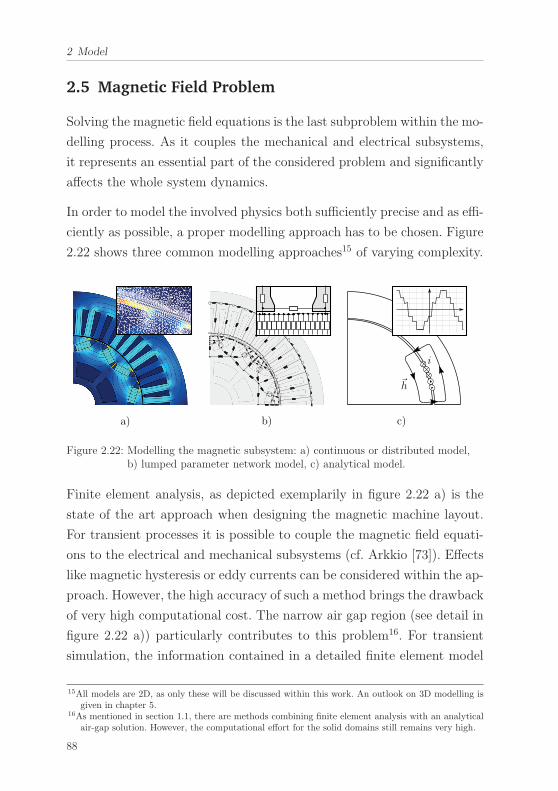
2 Model
2.5 Magnetic Field Problem
Solving the magnetic field equations is the last subproblem within the mo-
delling process. As it couples the mechanical and electrical subsystems,
it represents an essential part of the considered problem and significantly
affects the whole system dynamics.
In order to model the involved physics both sufficiently precise and as effi-
ciently as possible, a proper modelling approach has to be chosen. Figure
2.22 shows three common modelling approaches15 of varying complexity.
�h
i
a) b) c)
Figure 2.22: Modelling the magnetic subsystem: a) continuous or distributed model,b) lumped parameter network model, c) analytical model.
Finite element analysis, as depicted exemplarily in figure 2.22 a) is the
state of the art approach when designing the magnetic machine layout.
For transient processes it is possible to couple the magnetic field equati-
ons to the electrical and mechanical subsystems (cf. Arkkio [73]). Effects
like magnetic hysteresis or eddy currents can be considered within the ap-
proach. However, the high accuracy of such a method brings the drawback
of very high computational cost. The narrow air gap region (see detail in
figure 2.22 a)) particularly contributes to this problem16. For transient
simulation, the information contained in a detailed finite element model
15All models are 2D, as only these will be discussed within this work. An outlook on 3D modelling isgiven in chapter 5.
16As mentioned in section 1.1, there are methods combining finite element analysis with an analyticalair-gap solution. However, the computational effort for the solid domains still remains very high.
88
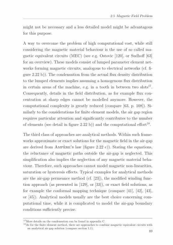
2.5 Magnetic Field Problem
might not be necessary and a less detailed model might be advantagous
for this purpose.
A way to overcome the problem of high computational cost, while still
considering the magnetic material behaviour is the use of so called ma-
gnetic equivalent circuits (MEC) (see e.g. Ostovic [120], or Sudhoff [63]
for an overview). These models consist of lumped parameter element net-
works forming magnetic circuits, analogous to electrical networks (cf. fi-
gure 2.22 b)). The condensation from the actual flux density distribution
to the lumped elements implies assuming a homogenous flux distribution
in certain areas of the machine, e.g. in a tooth in between two slots17.
Consequently, details in the field distribution, as for example flux con-
centration at sharp edges cannot be modelled anymore. However, the
computational complexity is greatly reduced (compare [63, p. 108]). Si-
milarly to the considerations for finite element models, the air gap region
requires particular attention and significantly contributes to the number
of elements (see detail in figure 2.22 b)) and the computational effort18.
The third class of approaches are analytical methods. Within such frame-
works approximate or exact solutions for the magnetic field in the air-gap
are derived from Ampere’s law (figure 2.22 c)). Stating the equations,
the reluctance of magnetic paths outside the air-gap is neglected. This
simplification also implies the neglection of any magnetic material beha-
viour. Therefore, such approaches cannot model magnetic non-linearities,
saturation or hysteresis effects. Typical examples for analytical methods
are the air-gap permeance method (cf. [23]), the modified winding func-
tion approach (as presented in [129], or [33]), or exact field solutions, as
for example the conformal mapping technique (compare [41], [42], [43],
or [45]). Analytical models usually are the best choice concerning com-
putational time, while it is complicated to model the air-gap boundary
conditions sufficiently precise.
17More details on the condensation can be found in appendix C.18As for the finite element method, there are approaches to combine magnetic equivalent circuits with
an analytical air-gap solution (compare section 1.1).89
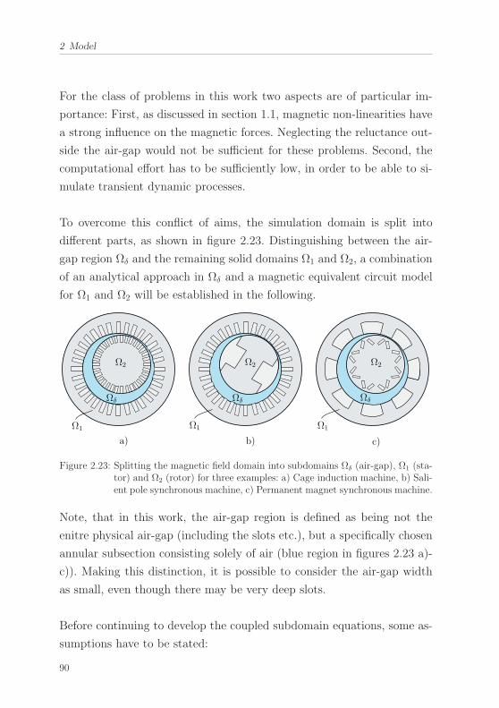
2 Model
For the class of problems in this work two aspects are of particular im-
portance: First, as discussed in section 1.1, magnetic non-linearities have
a strong influence on the magnetic forces. Neglecting the reluctance out-
side the air-gap would not be sufficient for these problems. Second, the
computational effort has to be sufficiently low, in order to be able to si-
mulate transient dynamic processes.
To overcome this conflict of aims, the simulation domain is split into
different parts, as shown in figure 2.23. Distinguishing between the air-
gap region Ωδ and the remaining solid domains Ω1 and Ω2, a combination
of an analytical approach in Ωδ and a magnetic equivalent circuit model
for Ω1 and Ω2 will be established in the following.
a) b) c)
Ω1 Ω1 Ω1
Ωδ ΩδΩδ
Ω2 Ω2 Ω2
Figure 2.23: Splitting the magnetic field domain into subdomains Ωδ (air-gap), Ω1 (sta-tor) and Ω2 (rotor) for three examples: a) Cage induction machine, b) Sali-ent pole synchronous machine, c) Permanent magnet synchronous machine.
Note, that in this work, the air-gap region is defined as being not the
enitre physical air-gap (including the slots etc.), but a specifically chosen
annular subsection consisting solely of air (blue region in figures 2.23 a)-
c)). Making this distinction, it is possible to consider the air-gap width
as small, even though there may be very deep slots.
Before continuing to develop the coupled subdomain equations, some as-
sumptions have to be stated:
90
2.5 Magnetic Field Problem
Assumptions 4: magnetic field
1. The magnetic field problem is considered two dimensional.This implies the neglection of axial phenomena such as ho-mopolar fluxes, or skewing.
2. All currents are assumed to flow perpendicular to the planeconsidered.
3. Eddy currents in solid conductive domains are neglected.
4. The distribution of currents in the conductors is assumed tobe homogenous. Therefore, skin and proximity effects are ne-glected.
5. It is assumed, that the minimal distance between the statorand rotor is small compared to the average of the largest rotorradius and the smallest stator bore radius.
6. Currents flowing in the electric circuits are assumed to passthe magnetic field domain once in positive and once in negativedirection, such that the resulting current linkage is zero.
7. It is assumed, that the solid domains can be subdivided intoregions, where the flux density is sufficiently homogenouslydistributed in order to approximate the field solution usingmean values.
8. The magnetic permeability is assumed to be isotropic.
9. Permanent magnets are assumed to exhibit a constant rema-nent flux density and an approximatlely linear magnetic cha-racteristic.
91
2 Model
Assumptions 1.1 and 1.2 ensure, that the problem can be considered
two dimensional. The neglection of eddy currents, skin and proximity ef-
fects (assumption 1.3 and 1.4) are simplifications, which are made to
reduce the problem in complexity. Especially the skin effect takes a cen-
tral role in strongly transient situations. Therefore, it should be included
in later studies.
Assumptions 4.5 and 4.6 are necessary for the air-gap field solution.
The first of these propositions is valid for most machine types. It should
be noted, that the gap, which is assumed to be small, is the distance of
the artificially chosen air-gap domain and does not include the much lar-
ger clearance, where slots are present. The second of these assumptions
assures the existence of a scalar magnetic potential in the air-gap domain.
The remaining assumptions 4.7 - 4.9 are stated in order to justify
the use of magnetic equivalent circuits. Although they impose certain re-
strictions on the field, it will be shown in chapter 3 that the equivalent
network combined with the analytical air-gap solution yields accurate re-
sults compared to a finite element model.
The following derivation of the magnetic field equations in each subdo-
main is done in two steps: First, the field problem in the air-gap is solved
approximately, based on an asymptotic expansion. In this context,
particularities concerning the solution and the consideration of slotting
effects and saliency are discussed. The second step involves the discretisa-
tion of the field equations for the use of magnetic equivalent circuits.
Furthermore, the derivation of network equations describing the problem
and the coupling with the air-gap field are explained here. The section
closes with some conclusions on the derived equations.
92
2.5 Magnetic Field Problem
2.5.1 Air-Gap Domain (Asymptotic Expansion)
The air-gap domain takes an essential role in the solution of the magnetic
field problem, as all energy converted from the electrical to the mecha-
nical subsystem and vice versa is transmitted through it. Over the last
decades, many different analytical solution techniques have been establis-
hed and applied to a vast number of problems.
The approach chosen in this work is an asymptotic expansion of the
field equations, which has been presented in detail in [48] and is summari-
sed in appendix B. This approach offers a straight forward mathematical
procedure to derive a simple approximative solution for the original field
problem. It is shown that for the first order approximation within this ap-
proach the radial component br of the flux density coincides with the well
known air-gap permeance method (compare Dorrell [23]). Furthermore,
also the tangential part bt can be calculated and the derivation mathe-
matically clearifies the order of magnitude of the flux density components.
The advantage of deriving the field solution by an asymptotic expansion
lies in the fact, that the solution is stated in terms of a magnetic poten-
tial. This allows for a simple establishment of the magnetic (co-)energy.
Furthermore the derivation does not rely on flux paths crossing the solid
domain. Therefore, the definition of transitional conditions towards the
stator and rotor is simplified and the magnetomotive force (MMF) is not
necessarily associated directly to the currents flowing within slots adja-
cent to the air-gap.
From a theoretical point of view, the asymptotic expansion allows for an
estimation of the involved error and a possibility to derive higher order
approximations19. Compared to exact solution techniques using a confor-
mal mapping [41–43, 45] it allows for very clearly arranged expressions.
19For the simulations in this work, a first order approximation is used.
93
2 Model
Therefore, it offers a simple way to derive the electromechanical coupling
in terms of integrals of the field solution.
This subsection is organised as follows: first, the general field problem is
analysed in terms of choosing a suitable magnetic potential and in terms
of stating transitional conditions towards the solid domains. Second, the
kinematics for the description of the fields considering rotor eccentricity
are introduced. Third, the results of the asymptotic approximation are
outlined and finally, an extension of the established approximation to ac-
count for slotting effects is presented.
General Field Problem
The equations describing the magnetic field problem in the air-gap do-
main areAmpere’s andGauß’ law of magnetostatics (equations (2.15a)).
They have to be accompanied by transitional/boundary conditions to cou-
ple the field to the surrounding solid domains.
As there are no current densities present in the air-gap, it is possible
to introduce magnetic potentials for both magnetic field equations (cf.
Rothwell and Cloud [111, p. 157-162]), based on Helmholtz’ theorem.
They are defined as
�h = −∇F , and �b = ∇× �a. (2.75)
For the problems considered within this work, the magnetic scalar poten-
tial F offers some advantages for the approximation of the air-gap field
problem. Therefore, it is chosen for all further considerations. A more
detailed discussion on this choice is given at the end of appendix B.
For the potential to exist, the integral condition∮C�h · d�s =
∫S�j · �n dA !
= 0 (2.76)
94
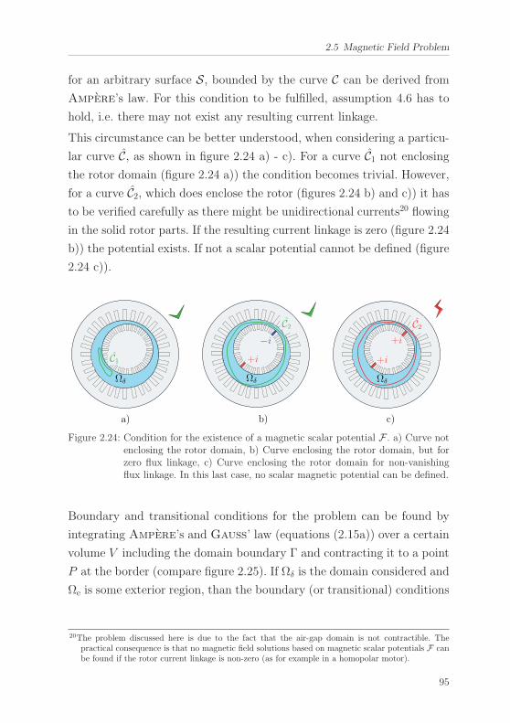
2.5 Magnetic Field Problem
for an arbitrary surface S, bounded by the curve C can be derived from
Ampere’s law. For this condition to be fulfilled, assumption 4.6 has to
hold, i.e. there may not exist any resulting current linkage.
This circumstance can be better understood, when considering a particu-
lar curve C, as shown in figure 2.24 a) - c). For a curve C1 not enclosing
the rotor domain (figure 2.24 a)) the condition becomes trivial. However,
for a curve C2, which does enclose the rotor (figures 2.24 b) and c)) it has
to be verified carefully as there might be unidirectional currents20 flowing
in the solid rotor parts. If the resulting current linkage is zero (figure 2.24
b)) the potential exists. If not a scalar potential cannot be defined (figure
2.24 c)).
Ωδ
C1Ωδ
C2
Ωδ
C2
+i
−i+i
+i
a) b) c)
Figure 2.24: Condition for the existence of a magnetic scalar potential F . a) Curve notenclosing the rotor domain, b) Curve enclosing the rotor domain, but forzero flux linkage, c) Curve enclosing the rotor domain for non-vanishingflux linkage. In this last case, no scalar magnetic potential can be defined.
Boundary and transitional conditions for the problem can be found by
integrating Ampere’s and Gauß’ law (equations (2.15a)) over a certain
volume V including the domain boundary Γ and contracting it to a point
P at the border (compare figure 2.25). If Ωδ is the domain considered and
Ωe is some exterior region, than the boundary (or transitional) conditions
20The problem discussed here is due to the fact that the air-gap domain is not contractible. Thepractical consequence is that no magnetic field solutions based on magnetic scalar potentials F canbe found if the rotor current linkage is non-zero (as for example in a homopolar motor).
95
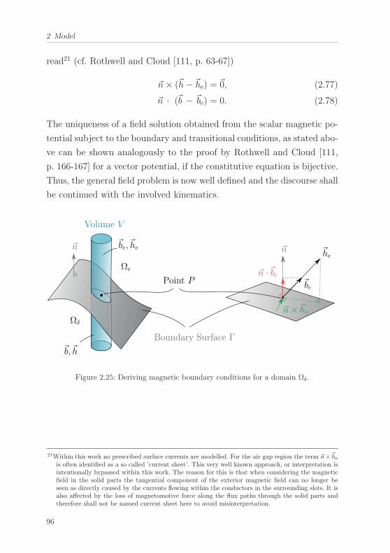
2 Model
read21 (cf. Rothwell and Cloud [111, p. 63-67])
�n× (�h− �he) = �0, (2.77)
�n · (�b − �be) = 0. (2.78)
The uniqueness of a field solution obtained from the scalar magnetic po-
tential subject to the boundary and transitional conditions, as stated abo-
ve can be shown analogously to the proof by Rothwell and Cloud [111,
p. 166-167] for a vector potential, if the constitutive equation is bijective.
Thus, the general field problem is now well defined and the discourse shall
be continued with the involved kinematics.
�n
Ωe
Ωδ
�be,�he
�b,�h
Volume V
�n
Point P �be
�he
�n ·�be
�n× �he
Boundary Surface Γ
Figure 2.25: Deriving magnetic boundary conditions for a domain Ωδ.
21Within this work no prescribed surface currents are modelled. For the air gap region the term �n×�heis often identified as a so called ’current sheet’. This very well known approach, or interpretation isintentionally bypassed within this work. The reason for this is that when considering the magneticfield in the solid parts the tangential component of the exterior magnetic field can no longer beseen as directly caused by the currents flowing within the conductors in the surrounding slots. It isalso affected by the loss of magnetomotive force along the flux paths through the solid parts andtherefore shall not be named current sheet here to avoid misinterpretation.
96
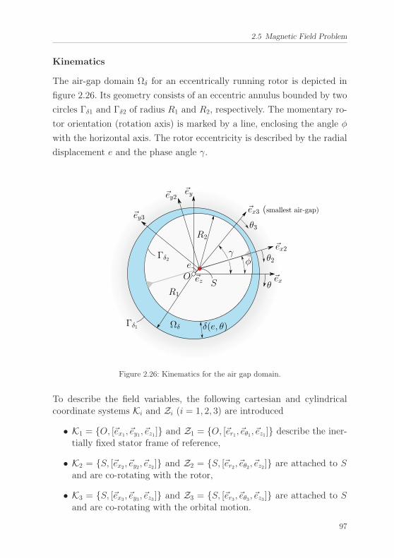
2.5 Magnetic Field Problem
Kinematics
The air-gap domain Ωδ for an eccentrically running rotor is depicted in
figure 2.26. Its geometry consists of an eccentric annulus bounded by two
circles Γδ1 and Γδ2 of radius R1 and R2, respectively. The momentary ro-
tor orientation (rotation axis) is marked by a line, enclosing the angle φ
with the horizontal axis. The rotor eccentricity is described by the radial
displacement e and the phase angle γ.
�ex
�ey
�ez SOe φ
γ
ΩδΓδ1
Γδ2
R2
R1
�ey2
�ex2
�ex3 (smallest air-gap)
δ(e, θ)
θ
θ2
θ3�ey3
Figure 2.26: Kinematics for the air gap domain.
To describe the field variables, the following cartesian and cylindricalcoordinate systems Ki and Zi (i = 1, 2, 3) are introduced
• K1 = {O, [�ex1, �ey1, �ez1]} and Z1 = {O, [�er1, �eθ1, �ez1]} describe the iner-tially fixed stator frame of reference,
• K2 = {S, [�ex2, �ey2, �ez2]} and Z2 = {S, [�er2, �eθ2, �ez2]} are attached to Sand are co-rotating with the rotor,
• K3 = {S, [�ex3, �ey3, �ez3]} and Z3 = {S, [�er3, �eθ3, �ez3]} are attached to Sand are co-rotating with the orbital motion.
97
2 Model
In the later description all variables are expressed with respect to the
inertial stator fixed cylindrical coordinate system Z1 and the subscript
1 is omitted for simplicity. As a peculiarity in this work, the orientation
of the coordinate θ is defined mathematically negative. This definition
allows for a simplified treatment of the magnetomotive force, which will
be explained later in this subsection.
If the rotor is centred (e = 0), the nominal air-gap width is δ0 = R1−R2.
For the eccentric rotor, the actual air-gap width δ reads
δ = δ0 − e cos(θ + γ) +R2
(1−√1−(e
R2
)2
sin2(θ + γ)
). (2.79)
Based on this formula, the rotor surface parametrised with respect to the
stator frame reads
R2δ = R1 − δ = e cos(θ + γ) +√R2
2 − e2 sin(θ + γ)2. (2.80)
Asymptotic Field Expansion
The partial differential equation governing the air-gap field problem re-
sults from Ampere’s law (first equation in (2.15a)) and the definition of
the scalar magnetic potential (first equation in (2.75)) and reads
ΔF = 0. (2.81)
To expand the potential asymptotically a small parameter ε must be cho-
sen. A natural choice for this number is the relation ε = δ0R2
between the
nominal air-gap width δ0 and the inner boundary radius R2. This para-
meter can be directly identified when describing the kinematics of the
problem and is purely geometrical22. Its order of magnitude varies bet-
22In a publication of Kim and Lieu [47], a similar expansion has been presented. Here, the relationbetween eccentricity e and inner boundary radius R2 has been proposed as a small parameter.However, this choice imposes several drawbacks. First, the small parameter varies in time if theeccentricity varies in time. Second, the expansion becomes trivial if the eccentricity tends towardszero, as F = F (0) + e
δ0F (1) + ... . And third, such an expansion yields a problem, which is linearised
98
2.5 Magnetic Field Problem
ween 10−3 to 10−2, depending on the machine type considered.
When expanding the magnetomotive force asymptotically according to
F = F{0} + εF{1} + ...+O(εn), (2.82)
and inserting it into equation (2.81), the first order solution F{0} subjectto the boundary conditions (2.77) is found as
F{0} = −(f1 + f2)(r −R2δ
δ
)+ f2, (2.83)
(compare (B.8)), where
f1(θ, t) = −∫Γδ1
(�n× �he1) · �ez R dθ︸ ︷︷ ︸fe1(θ,t)
+f0(t), (2.84a)
f2(θ, t) =
∫Γδ2
(�n× �he2) · �ez R dθ︸ ︷︷ ︸fe2(θ,t)
. (2.84b)
Both equations above are stated using the mean nominal air-gap radius
R = R1+R2
2 . Certainly, when deriving the boundary conditions exactly, the
radius R1 would have to be used for the stator side and R2δ for the rotor
surface. However, the error made when using the mean radius instead
of the individual radii is of order O(ε) (compare (B.14)). Therefore, this
mean nominal radius is used here and in the following for all first order
approximations.
The variable f0(t) is a spatial constant of integration, enforcing Gauß’
law (second equation in (2.15a)) to be fulfilled (compare (B.13)).
Having defined the potential, the approximation of the magnetic flux
with respect to e and thus is valid only for small eccentricities and thus small lateral oscillations.
99
2 Model
density can be found conveniently using definition (2.75), reading
�b = −μ0(∂F{0}
∂r�er +
1
r
∂F{0}
∂θ�eθ
)= b{0}r �er + b
{1}θ �eθ +O(ε2), (2.85a)
where
b{0}r =μ0δ
(f1 + f2
)= Λf, (2.85b)
b{1}θ = −μ0
R
(∂(f1 + f2)
∂θ
(r −R2δ
δ
)− ∂f2
∂θ
). (2.85c)
The radial component in this result coincides with the well known air-gap
permeance formulation. In this sense Λ = μ0
δ is the air-gap permeance and
f = f1 + f2 is the resulting air-gap boundary MMF. It is important to
note that there is a tangential field component, although it is one order
of magnitude smaller than the radial one.
In the following, only first order approximations are considered. Therefo-
re, the superscript is omitted (i.e. F = F{0}), implying an approximation
error of order O(ε). For higher order approximations, refer to [48].
As a further task, the spatial integration constant f0(t) has to be defined.
To this end, Gauß’ law is integrated over to the entire air-gap and rotor
volume ∫Ωδ∪Ω2
∇ ·�b dV =
∮Γ1
�b · �n︸︷︷︸=br
dS!= 0,
where Gauß’ theorem has been applied. Substituting (2.84a) and (2.85)
yields ∫ π
−π
μ0δ(fe1 + f0 + fe2) �Rdθ
!= 0
In this context, � is the effective magnetic length in axial direction (com-
100
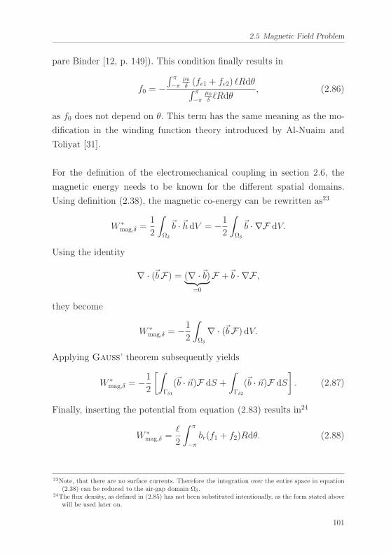
2.5 Magnetic Field Problem
pare Binder [12, p. 149]). This condition finally results in
f0 = −∫ π−π
μ0
δ (fe1 + fe2) �Rdθ∫ π−π
μ0
δ �Rdθ, (2.86)
as f0 does not depend on θ. This term has the same meaning as the mo-
dification in the winding function theory introduced by Al-Nuaim and
Toliyat [31].
For the definition of the electromechanical coupling in section 2.6, the
magnetic energy needs to be known for the different spatial domains.
Using definition (2.38), the magnetic co-energy can be rewritten as23
W ∗mag,δ =
1
2
∫Ωδ
�b · �h dV = −1
2
∫Ωδ
�b · ∇F dV.
Using the identity
∇ · (�bF) = (∇ ·�b)︸ ︷︷ ︸=0
F +�b · ∇F ,
they become
W ∗mag,δ = −1
2
∫Ωδ
∇ · (�bF) dV.
Applying Gauß’ theorem subsequently yields
W ∗mag,δ = −1
2
[∫Γδ1
(�b · �n)F dS +
∫Γδ2
(�b · �n)F dS
]. (2.87)
Finally, inserting the potential from equation (2.83) results in24
W ∗mag,δ =
�
2
∫ π
−πbr(f1 + f2)Rdθ. (2.88)
23Note, that there are no surface currents. Therefore the integration over the entire space in equation(2.38) can be reduced to the air-gap domain Ωδ.
24The flux density, as defined in (2.85) has not been substituted intentionally, as the form stated abovewill be used later on.
101
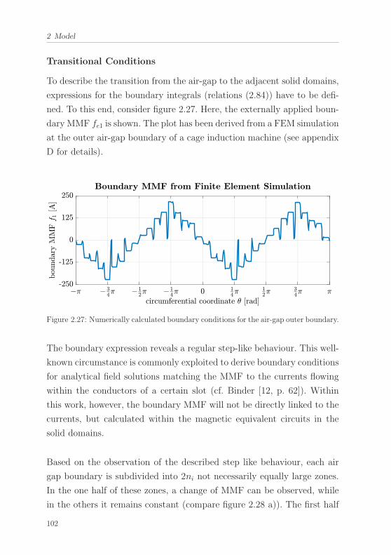
2 Model
Transitional Conditions
To describe the transition from the air-gap to the adjacent solid domains,
expressions for the boundary integrals (relations (2.84)) have to be defi-
ned. To this end, consider figure 2.27. Here, the externally applied boun-
dary MMF fe1 is shown. The plot has been derived from a FEM simulation
at the outer air-gap boundary of a cage induction machine (see appendix
D for details).
Figure 2.27: Numerically calculated boundary conditions for the air-gap outer boundary.
The boundary expression reveals a regular step-like behaviour. This well-
known circumstance is commonly exploited to derive boundary conditions
for analytical field solutions matching the MMF to the currents flowing
within the conductors of a certain slot (cf. Binder [12, p. 62]). Within
this work, however, the boundary MMF will not be directly linked to the
currents, but calculated within the magnetic equivalent circuits in the
solid domains.
Based on the observation of the described step like behaviour, each air
gap boundary is subdivided into 2ni not necessarily equally large zones.
In the one half of these zones, a change of MMF can be observed, while
in the others it remains constant (compare figure 2.28 a)). The first half
102
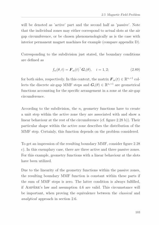
2.5 Magnetic Field Problem
will be denoted as ’active’ part and the second half as ’passive’. Note
that the individual zones may either correspond to actual slots at the air
gap circumference, or be chosen phenomenologically as is the case with
interior permanent magnet machines for example (compare appendix D).
Corresponding to the subdivision just stated, the boundary conditions
are defined as
fei(θ, t) = F ai(t)�Gi(θ), i = 1, 2; (2.89)
for both sides, respectively. In this context, the matrix F ai(t) ∈ Rni×1 col-
lects the discrete air-gap MMF steps and Gi(θ) ∈ Rni×1 are geometrical
functions accounting for the specific arrangement in a zone at the air-gap
circumference.
According to the subdivision, the ni geometry functions have to create
a unit step within the active zone they are associated with and show a
linear behaviour at the rest of the circumference (cf. figure 2.28 b)). Their
particular shape within the active zone describes the distribution of the
MMF step. Certainly, this function depends on the problem considered.
To get an impression of the resulting boundary MMF, consider figure 2.28
c). In this exemplary case, there are three active and three passive zones.
For this example, geometry functions with a linear behaviour at the slots
have been utilized.
Due to the linearity of the geometry functions within the passive zones,
the resulting boundary MMF function is constant within these parts if
the sum of MMF steps is zero. The latter condition is always fulfilled,
if Ampere’s law and assumption 4.6 are valid. This circumstance will
be important, when proving the equivalence between the classical and
analytical approach in section 2.6.
103
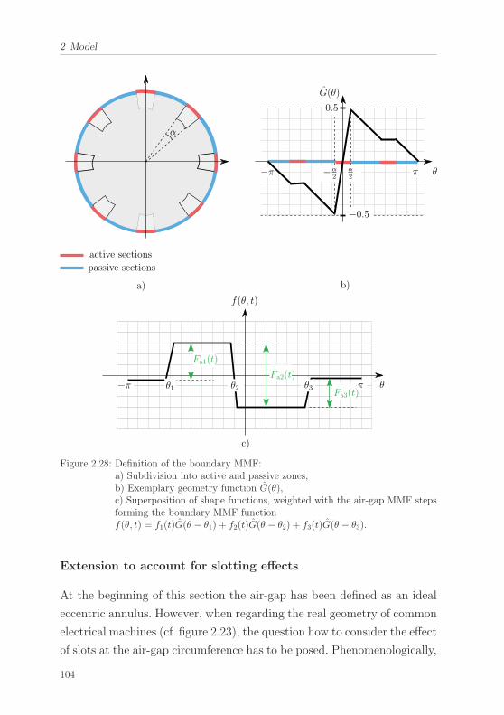
2 Model
a) b)
c)
active sections
passive sections
θ−α2
α2
α
0.5
−0.5
G(θ)
θ
f(θ, t)
θ2 θ3Fa3(t)
Fa1(t)
Fa2(t)−π θ1 π
π−π
Figure 2.28: Definition of the boundary MMF:a) Subdivision into active and passive zones,b) Exemplary geometry function G(θ),c) Superposition of shape functions, weighted with the air-gap MMF stepsforming the boundary MMF functionf(θ, t) = f1(t)G(θ − θ1) + f2(t)G(θ − θ2) + f3(t)G(θ − θ3).
Extension to account for slotting effects
At the beginning of this section the air-gap has been defined as an ideal
eccentric annulus. However, when regarding the real geometry of common
electrical machines (cf. figure 2.23), the question how to consider the effect
of slots at the air-gap circumference has to be posed. Phenomenologically,
104
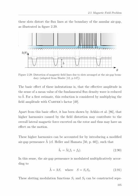
2.5 Magnetic Field Problem
these slots distort the flux lines at the boundary of the annular air-gap,
as illustrated in figure 2.29.
θ
b
b(θ)
Figure 2.29: Distortion of magnetic field lines due to slots arranged at the air-gap boun-dary (adapted from Binder [12, p.147]).
The basic effect of these indentations is, that the effective amplitude in
the sense of a mean value of the fundamental flux density wave is reduced
to b. For a first estimate, this reduction is considered by multiplying the
field amplitude with Carter’s factor [49].
Apart from this basic effect, it has been shown by Arkkio et al. [86], that
higher harmonics caused by the field distortion may contribute to the
overall lateral magnetic force excerted on the rotor and thus may have an
effect on the motion.
These higher harmonics can be accounted for by introducing a modified
air-gap permeance Λ (cf. Heller and Hamata [50, p. 60]), such that
br = Λ(f1 + f2). (2.90)
In this sense, the air-gap permeance is modulated multiplicatively accor-
ding to
Λ = ΛS, where S = S1S2. (2.91)
These slotting modulation functions S1 and S2 can be constructed sepe-
105
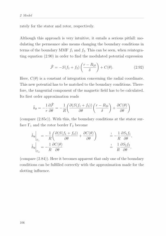
2 Model
rately for the stator and rotor, respectively.
Although this approach is very intuitive, it entails a serious pitfall: mo-
dulating the permeance also means changing the boundary conditions in
terms of the boundary MMF f1 and f2. This can be seen, when reintegra-
ting equation (2.90) in order to find the modulated potential expression
F = −S(f1 + f2)
(r −R2δ
δ
)+ C(θ). (2.92)
Here, C(θ) is a constant of integration concerning the radial coordinate.
This new potential has to be matched to the boundary conditions. There-
fore, the tangential component of the magnetic field has to be calculated.
Its first order approximation reads
hθ = −1
r
∂F∂θ
= − 1
R
(∂(S(f1 + f2))
∂θ
(r −R2δ
δ
)+∂C(θ)
∂θ
)
(compare (2.85c)). With this, the boundary conditions at the stator sur-
face Γ1 and the rotor border Γ2 become
hθ
∣∣∣∣Γ1
= − 1
R
(∂(S(f1 + f2))
∂θ+∂C(θ)
∂θ
)!= − 1
R
∂S1f1∂θ
,
hθ
∣∣∣∣Γ2
= − 1
R
∂C(θ)
∂θ!=
1
R
∂S2f2∂θ
,
(compare (2.84)). Here it becomes apparent that only one of the boundary
conditions can be fulfilled correctly with the approximation made for the
slotting influence.
106
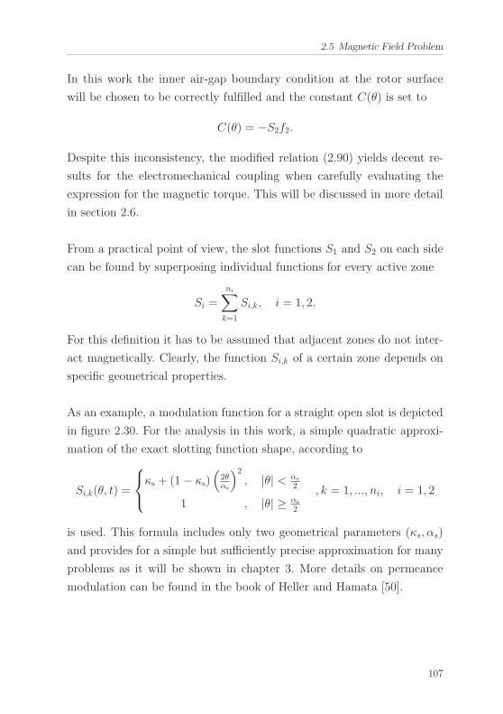
2.5 Magnetic Field Problem
In this work the inner air-gap boundary condition at the rotor surface
will be chosen to be correctly fulfilled and the constant C(θ) is set to
C(θ) = −S2f2.
Despite this inconsistency, the modified relation (2.90) yields decent re-
sults for the electromechanical coupling when carefully evaluating the
expression for the magnetic torque. This will be discussed in more detail
in section 2.6.
From a practical point of view, the slot functions S1 and S2 on each side
can be found by superposing individual functions for every active zone
Si =
ni∑k=1
Si,k, i = 1, 2.
For this definition it has to be assumed that adjacent zones do not inter-
act magnetically. Clearly, the function Si,k of a certain zone depends on
specific geometrical properties.
As an example, a modulation function for a straight open slot is depicted
in figure 2.30. For the analysis in this work, a simple quadratic approxi-
mation of the exact slotting function shape, according to
Si,k(θ, t) =
⎧⎨⎩κs + (1− κs)
(2θαs
)2, |θ| < αs
2
1 , |θ| ≥ αs
2
, k = 1, ..., ni, i = 1, 2
is used. This formula includes only two geometrical parameters (κs, αs)
and provides for a simple but sufficiently precise approximation for many
problems as it will be shown in chapter 3. More details on permeance
modulation can be found in the book of Heller and Hamata [50].
107
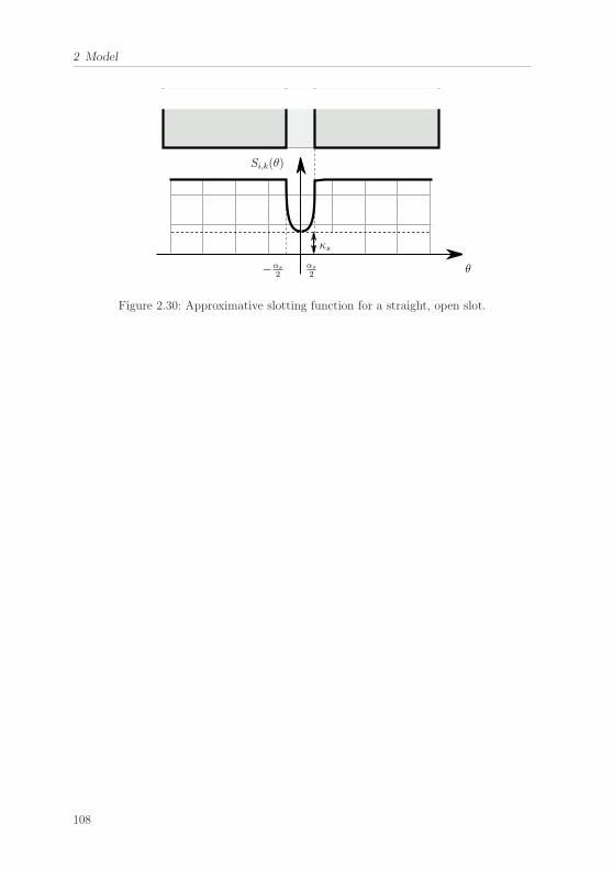
2 Model
θ
Si,k(θ)
αs
2−αs
2
κs
Figure 2.30: Approximative slotting function for a straight, open slot.
108
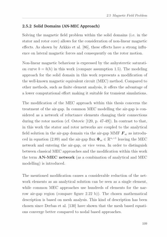
2.5 Magnetic Field Problem
2.5.2 Solid Domains (AN-MEC Approach)
Solving the magnetic field problem within the solid domains (i.e. in the
stator and rotor core) allows for the consideration of non-linear magnetic
effects. As shown by Arkkio et al. [86], these effects have a strong influ-
ence on lateral magnetic forces and consequently on the rotor motion.
Non-linear magnetic behaviour is expressed by the anhysteretic saturati-
on curve b = b(h) in this work (compare assumption 1.5). The modeling
approach for the solid domain in this work represents a modification of
the well-known magnetic equivalent circuit (MEC) method. Compared to
other methods, such as finite element analysis, it offers the advantage of
a lower computational effort making it suitable for transient simulations.
The modification of the MEC approach within this thesis concerns the
treatment of the air-gap. In common MEC modelling the air-gap is con-
sidered as a network of reluctance elements changing their connections
during the rotor motion (cf. Ostovic [120, p. 47-49]). In contrast to that,
in this work the stator and rotor networks are coupled to the analytical
field solution in the air-gap domain via the air-gap MMF F ai as introdu-
ced in equation (2.89) and the air-gap flux Φai ∈ Rni×1 leaving the MEC
network and entering the air-gap, or vice versa. In order to distinguish
between classical MEC approaches and the modification within this work
the term AN-MEC network (as a combination of analytical and MEC
modelling) is introduced.
The mentioned modification causes a considerable reduction of the net-
work elements as an analytical solution can be seen as a single element,
while common MEC approaches use hundreds of elements for the nar-
row air-gap region (compare figure 2.22 b)). The chosen mathematical
description is based on mesh analysis. This kind of description has been
chosen since Derbas et al. [130] have shown that the mesh based equati-
ons converge better compared to nodal based approaches.
109
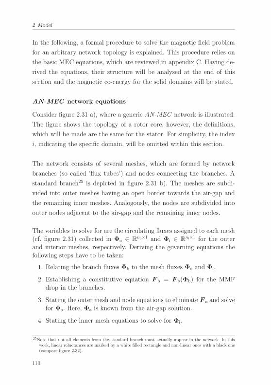
2 Model
In the following, a formal procedure to solve the magnetic field problem
for an arbitrary network topology is explained. This procedure relies on
the basic MEC equations, which are reviewed in appendix C. Having de-
rived the equations, their structure will be analysed at the end of this
section and the magnetic co-energy for the solid domains will be stated.
AN-MEC network equations
Consider figure 2.31 a), where a generic AN-MEC network is illustrated.
The figure shows the topology of a rotor core, however, the definitions,
which will be made are the same for the stator. For simplicity, the index
i, indicating the specific domain, will be omitted within this section.
The network consists of several meshes, which are formed by network
branches (so called ’flux tubes’) and nodes connecting the branches. A
standard branch25 is depicted in figure 2.31 b). The meshes are subdi-
vided into outer meshes having an open border towards the air-gap and
the remaining inner meshes. Analogously, the nodes are subdivided into
outer nodes adjacent to the air-gap and the remaining inner nodes.
The variables to solve for are the circulating fluxes assigned to each mesh(cf. figure 2.31) collected in Φo ∈ R
no×1 and Φi ∈ Rni×1 for the outer
and interior meshes, respectively. Deriving the governing equations thefollowing steps have to be taken:
1. Relating the branch fluxes Φb to the mesh fluxes Φo and Φi.
2. Establishing a constitutive equation F b = F b(Φb) for the MMFdrop in the branches.
3. Stating the outer mesh and node equations to eliminate F a and solvefor Φo. Here, Φa is known from the air-gap solution.
4. Stating the inner mesh equations to solve for Φi.
25Note that not all elements from the standard branch must actually appear in the network. In thiswork, linear reluctances are marked by a white filled rectangle and non-linear ones with a black one(compare figure 2.32).
110
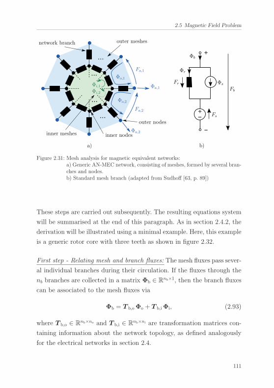
2.5 Magnetic Field Problem
a) b)
outer meshes
inner meshes inner nodes
outer nodes
network branch
Φo,1
Fa,1
Φi,1
Φo,2
Φi,2
Fa,2
Fr Φs
Fs
Fb
Φb
Φr
Φa,1
Φa,2
Figure 2.31: Mesh analysis for magnetic equivalent networks:a) Generic AN-MEC network, consisting of meshes, formed by several bran-ches and nodes.b) Standard mesh branch (adapted from Sudhoff [63, p. 89])
These steps are carried out subsequently. The resulting equations system
will be summarised at the end of this paragraph. As in section 2.4.2, the
derivation will be illustrated using a minimal example. Here, this example
is a generic rotor core with three teeth as shown in figure 2.32.
First step - Relating mesh and branch fluxes: The mesh fluxes pass sever-
al individual branches during their circulation. If the fluxes through the
nb branches are collected in a matrix Φb ∈ Rnb×1, then the branch fluxes
can be associated to the mesh fluxes via
Φb = T b,oΦo + T b,iΦi, (2.93)
where T b,o ∈ Rnb×no and T b,i ∈ R
nb×ni are transformation matrices con-
taining information about the network topology, as defined analogously
for the electrical networks in section 2.4.
111
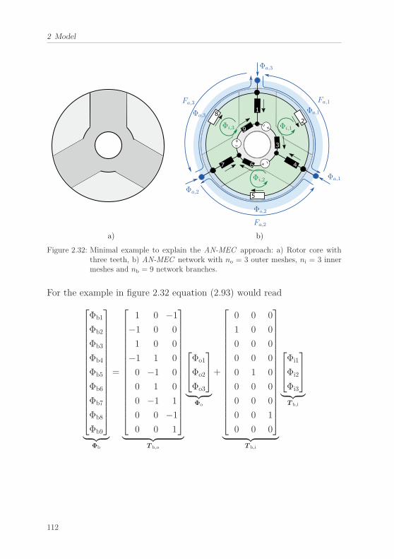
2 Model
a) b)
Φi,1
Φi,2
Φi,3
Fa,1Φo,1
Φo,2
Φo,3
Fa,2
Fa,3
Φa,3
Φa,1
Φa,2
Figure 2.32: Minimal example to explain the AN-MEC approach: a) Rotor core withthree teeth, b) AN-MEC network with no = 3 outer meshes, ni = 3 innermeshes and nb = 9 network branches.
For the example in figure 2.32 equation (2.93) would read⎡⎢⎢⎢⎢⎢⎢⎢⎢⎢⎢⎢⎢⎢⎢⎢⎢⎣
Φb1
Φb2
Φb3
Φb4
Φb5
Φb6
Φb7
Φb8
Φb9
⎤⎥⎥⎥⎥⎥⎥⎥⎥⎥⎥⎥⎥⎥⎥⎥⎥⎦
︸ ︷︷ ︸Φb
=
⎡⎢⎢⎢⎢⎢⎢⎢⎢⎢⎢⎢⎢⎢⎢⎢⎢⎣
1 0 −1
−1 0 0
1 0 0
−1 1 0
0 −1 0
0 1 0
0 −1 1
0 0 −1
0 0 1
⎤⎥⎥⎥⎥⎥⎥⎥⎥⎥⎥⎥⎥⎥⎥⎥⎥⎦
︸ ︷︷ ︸T b,o
⎡⎢⎣Φo1
Φo2
Φo3
⎤⎥⎦
︸ ︷︷ ︸Φo
+
⎡⎢⎢⎢⎢⎢⎢⎢⎢⎢⎢⎢⎢⎢⎢⎢⎢⎣
0 0 0
1 0 0
0 0 0
0 0 0
0 1 0
0 0 0
0 0 0
0 0 1
0 0 0
⎤⎥⎥⎥⎥⎥⎥⎥⎥⎥⎥⎥⎥⎥⎥⎥⎥⎦
︸ ︷︷ ︸T b,i
⎡⎢⎣Φi1
Φi2
Φi3
⎤⎥⎦
︸ ︷︷ ︸T b,i
112
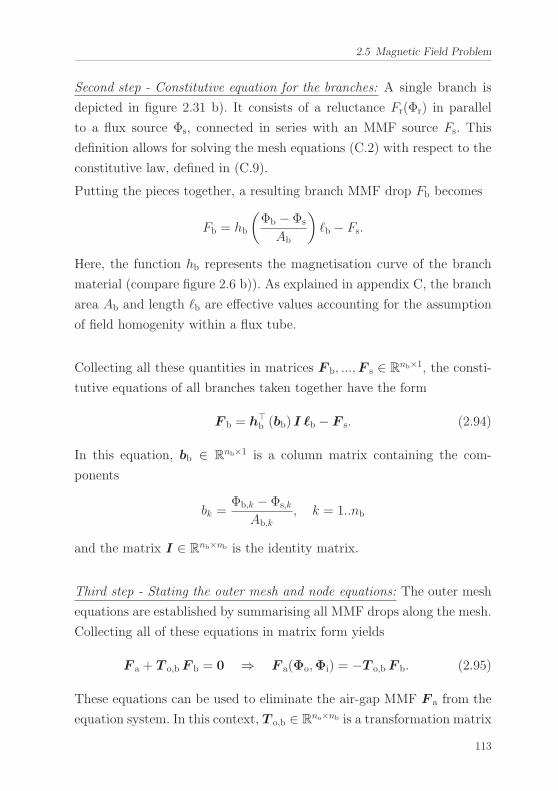
2.5 Magnetic Field Problem
Second step - Constitutive equation for the branches: A single branch is
depicted in figure 2.31 b). It consists of a reluctance Fr(Φr) in parallel
to a flux source Φs, connected in series with an MMF source Fs. This
definition allows for solving the mesh equations (C.2) with respect to the
constitutive law, defined in (C.9).
Putting the pieces together, a resulting branch MMF drop Fb becomes
Fb = hb
(Φb − Φs
Ab
)�b − Fs.
Here, the function hb represents the magnetisation curve of the branch
material (compare figure 2.6 b)). As explained in appendix C, the branch
area Ab and length �b are effective values accounting for the assumption
of field homogenity within a flux tube.
Collecting all these quantities in matrices F b, ...,F s ∈ Rnb×1, the consti-
tutive equations of all branches taken together have the form
F b = h�b (bb) I �b − F s. (2.94)
In this equation, bb ∈ Rnb×1 is a column matrix containing the com-
ponents
bk =Φb,k − Φs,k
Ab,k, k = 1..nb
and the matrix I ∈ Rnb×nb is the identity matrix.
Third step - Stating the outer mesh and node equations: The outer mesh
equations are established by summarising all MMF drops along the mesh.
Collecting all of these equations in matrix form yields
F a + T o,bF b = 0 ⇒ F a(Φo,Φi) = −T o,bF b. (2.95)
These equations can be used to eliminate the air-gap MMF F a from the
equation system. In this context, T o,b ∈ Rno×nb is a transformation matrix
113
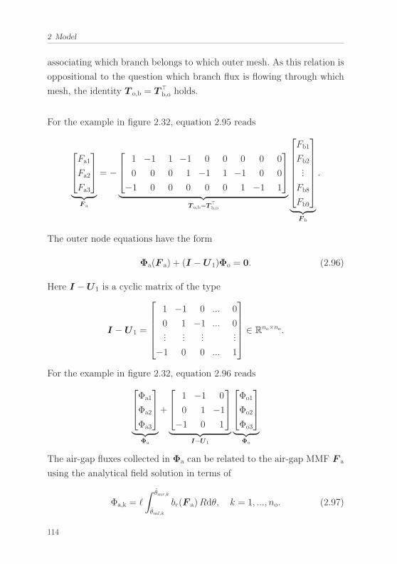
2 Model
associating which branch belongs to which outer mesh. As this relation is
oppositional to the question which branch flux is flowing through which
mesh, the identity T o,b = T�b,o holds.
For the example in figure 2.32, equation 2.95 reads
⎡⎢⎣Fa1
Fa2
Fa3
⎤⎥⎦
︸ ︷︷ ︸F a
= −
⎡⎢⎣ 1 −1 1 −1 0 0 0 0 0
0 0 0 1 −1 1 −1 0 0
−1 0 0 0 0 0 1 −1 1
⎤⎥⎦
︸ ︷︷ ︸T o,b=T�
b,o
⎡⎢⎢⎢⎢⎢⎢⎣
Fb1
Fb2...
Fb8
Fb9
⎤⎥⎥⎥⎥⎥⎥⎦
︸ ︷︷ ︸F b
.
The outer node equations have the form
Φa(F a) + (I −U 1)Φo = 0. (2.96)
Here I −U 1 is a cyclic matrix of the type
I −U 1 =
⎡⎢⎢⎢⎢⎣
1 −1 0 ... 0
0 1 −1 ... 0...
......
...
−1 0 0 ... 1
⎤⎥⎥⎥⎥⎦ ∈ R
no×no.
For the example in figure 2.32, equation 2.96 reads⎡⎢⎣Φa1
Φa2
Φa3
⎤⎥⎦
︸ ︷︷ ︸Φa
+
⎡⎢⎣ 1 −1 0
0 1 −1
−1 0 1
⎤⎥⎦
︸ ︷︷ ︸I−U1
⎡⎢⎣Φo1
Φo2
Φo3
⎤⎥⎦
︸ ︷︷ ︸Φo
The air-gap fluxes collected in Φa can be related to the air-gap MMF F a
using the analytical field solution in terms of
Φa,k = �
∫ θmr,k
θml,k
br(F a)Rdθ, k = 1, ..., no. (2.97)
114
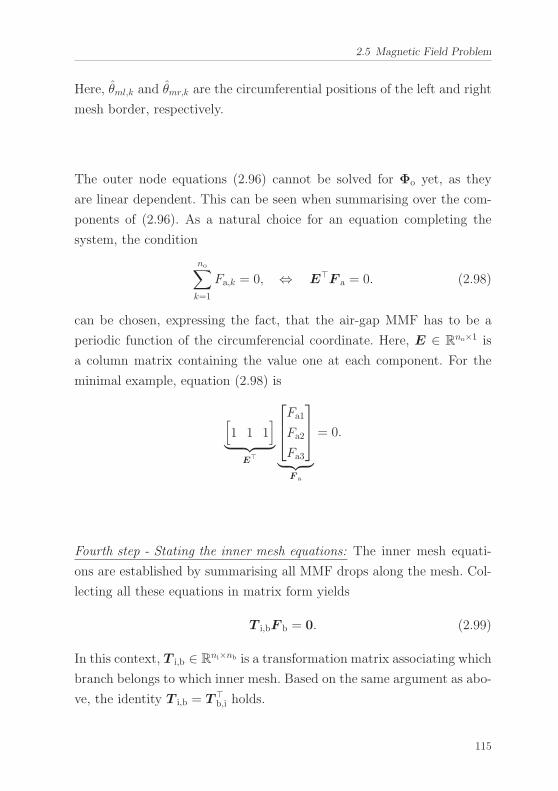
2.5 Magnetic Field Problem
Here, θml,k and θmr,k are the circumferential positions of the left and right
mesh border, respectively.
The outer node equations (2.96) cannot be solved for Φo yet, as they
are linear dependent. This can be seen when summarising over the com-
ponents of (2.96). As a natural choice for an equation completing the
system, the condition
no∑k=1
Fa,k = 0, ⇔ E�F a = 0. (2.98)
can be chosen, expressing the fact, that the air-gap MMF has to be a
periodic function of the circumferencial coordinate. Here, E ∈ Rno×1 is
a column matrix containing the value one at each component. For the
minimal example, equation (2.98) is
[1 1 1
]︸ ︷︷ ︸
E�
⎡⎢⎣Fa1
Fa2
Fa3
⎤⎥⎦
︸ ︷︷ ︸F a
= 0.
Fourth step - Stating the inner mesh equations: The inner mesh equati-
ons are established by summarising all MMF drops along the mesh. Col-
lecting all these equations in matrix form yields
T i,bF b = 0. (2.99)
In this context, T i,b ∈ Rni×nb is a transformation matrix associating which
branch belongs to which inner mesh. Based on the same argument as abo-
ve, the identity T i,b = T�b,i holds.
115
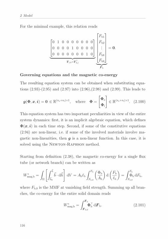
2 Model
For the minimal example, this relation reads
⎡⎢⎣0 1 0 0 0 0 0 0 0
0 0 0 0 1 0 0 0 0
0 0 0 0 0 0 0 1 0
⎤⎥⎦
︸ ︷︷ ︸T i,b=T�
b,i
⎡⎢⎢⎢⎢⎢⎢⎣
Fb1
Fb2...
Fb8
Fb9
⎤⎥⎥⎥⎥⎥⎥⎦
︸ ︷︷ ︸F b
= 0.
Governing equations and the magnetic co-energy
The resulting equation system can be obtained when substituting equa-
tions (2.93)-(2.95) and (2.97) into (2.96),(2.98) and (2.99). This leads to
g(Φ,x, i) = 0 ∈ R(no+ni)×1, where Φ =
[Φo
Φi
]∈ R
(no+ni)×1. (2.100)
This equation system has two important peculiarities in view of the entire
system dynamics: first, it is an implicit algebraic equation, which defines
Φ(x, i) in each time step. Second, if some of the constitutive equations
(2.94) are non-linear, i.e. if some of the involved materials involve ma-
gnetic non-linearities, then g is a non-linear function. In this case, it is
solved using the Newton-Raphson method.
Starting from definition (2.38), the magnetic co-energy for a single flux
tube (or network branch) can be written as
W ∗mag,b =
∫Ω
[∫ �h
�h0
�b · d�h]dV = Ab�b
∫ Fb
Fb,0
(Φb
Ab
)d
(Fb
�b
)=
∫ Fb
Fb,0
Φb dFb,
where Fb,0 is the MMF at vanishing field strength. Summing up all bran-
ches, the co-energy for the entire solid domain reads
W ∗mag,b =
∫ F b
F b,0
Φ�b dF b. (2.101)
116
2.5 Magnetic Field Problem
2.5.3 Conclusions
To end the section on the magnetic field problem, the following conclusi-
ons can be drawn
Conclusions 4: Magnetic Field Problem
1. In order to meet the requirements of providing sufficient ac-curacy while maintaining a high numerical efficiency, a combi-nation of an analytical field solution in the air-gap and a mo-dified magnetic equivalent circuit approach for solid domainshas been developed in this work.
2. The air-gap field has been approximated by an asymptoticexpansion of the scalar magnetic potential. The radial com-ponent of the flux density for the chosen first order approachcoincides with the well known air-gap permeance formulation.Additionally, there is a tangential component, satisfying theboundary conditions.
3. The asymptotic solution for the air-gap field can be modulatedto account for the effect of slots. This modulation is realisedby modulating the permeance in the radial component of theflux density and the boundary conditions.
4. In contrast to classical approaches, the boundary MMF in thiswork is calculated from magnetic equivalent networks withinthe solid parts. In return the flux entering the rotor and statorcan be calculated from the analytical air-gap solution.
5. The modified network method (AN-MEC approach) dis-tinguishes between outer and inner mesh and node equations.Outer nodes and meshes share a common border with the air-gap. Inner equations form the remainder.
6. The resulting magnetic equation system is non-linear and al-gebraic. It must be solved in each time step.
117
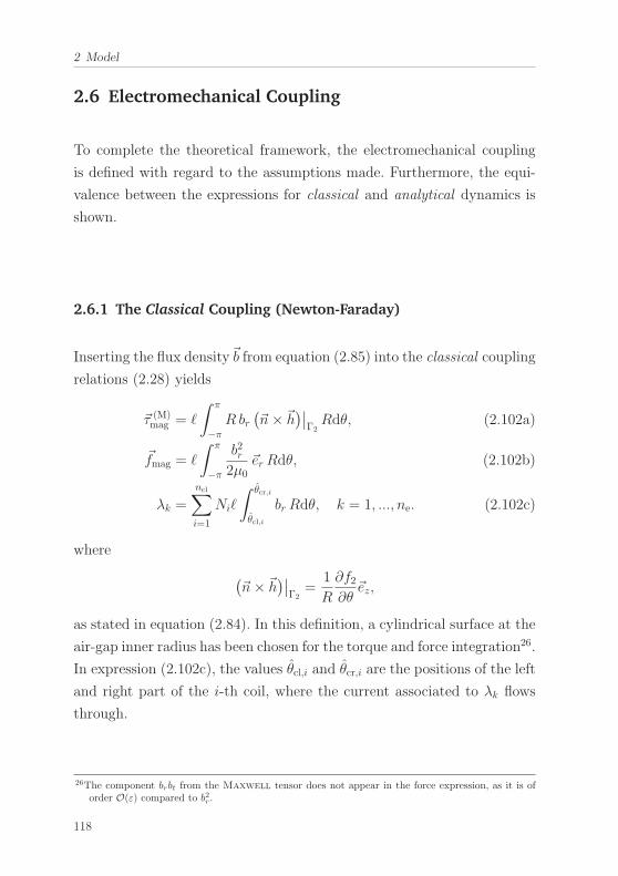
2 Model
2.6 Electromechanical Coupling
To complete the theoretical framework, the electromechanical coupling
is defined with regard to the assumptions made. Furthermore, the equi-
valence between the expressions for classical and analytical dynamics is
shown.
2.6.1 The Classical Coupling (Newton-Faraday)
Inserting the flux density�b from equation (2.85) into the classical coupling
relations (2.28) yields
�τ (M)mag = �
∫ π
−πR br
(�n× �h
)∣∣Γ2Rdθ, (2.102a)
�fmag = �
∫ π
−π
b2r2μ0
�erRdθ, (2.102b)
λk =
ncl∑i=1
Ni�
∫ θcr,i
θcl,i
brRdθ, k = 1, ..., ne. (2.102c)
where
(�n× �h
)∣∣Γ2
=1
R
∂f2∂θ
�ez,
as stated in equation (2.84). In this definition, a cylindrical surface at the
air-gap inner radius has been chosen for the torque and force integration26.
In expression (2.102c), the values θcl,i and θcr,i are the positions of the left
and right part of the i-th coil, where the current associated to λk flows
through.
26The component brbt from the Maxwell tensor does not appear in the force expression, as it is oforder O(ε) compared to b2r.
118
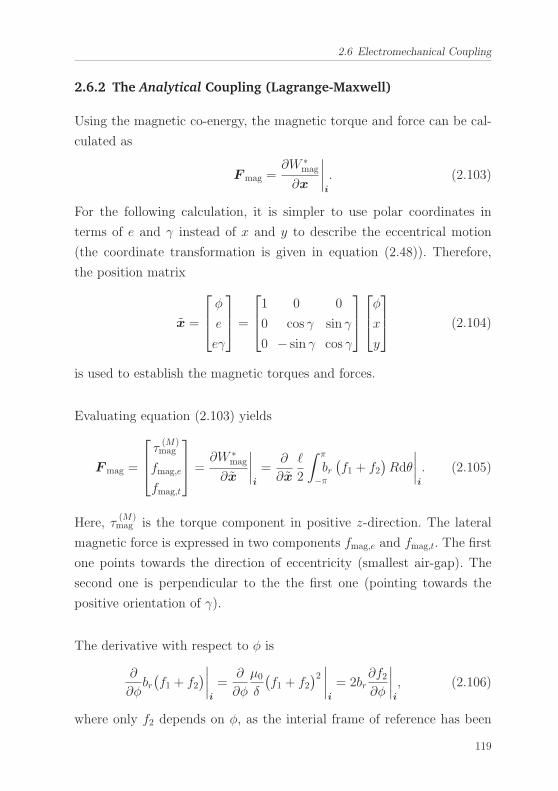
2.6 Electromechanical Coupling
2.6.2 The Analytical Coupling (Lagrange-Maxwell)
Using the magnetic co-energy, the magnetic torque and force can be cal-
culated as
Fmag =∂W ∗
mag
∂x
∣∣∣∣i
. (2.103)
For the following calculation, it is simpler to use polar coordinates in
terms of e and γ instead of x and y to describe the eccentrical motion
(the coordinate transformation is given in equation (2.48)). Therefore,
the position matrix
x =
⎡⎢⎣ φeeγ
⎤⎥⎦ =
⎡⎢⎣1 0 0
0 cos γ sin γ
0 − sin γ cos γ
⎤⎥⎦⎡⎢⎣φxy
⎤⎥⎦ (2.104)
is used to establish the magnetic torques and forces.
Evaluating equation (2.103) yields
Fmag =
⎡⎢⎣ τ
(M)mag
fmag,e
fmag,t
⎤⎥⎦ =
∂W ∗mag
∂x
∣∣∣∣i
=∂
∂x
�
2
∫ π
−πbr(f1 + f2
)Rdθ
∣∣∣∣i
. (2.105)
Here, τ(M)mag is the torque component in positive z-direction. The lateral
magnetic force is expressed in two components fmag,e and fmag,t. The first
one points towards the direction of eccentricity (smallest air-gap). The
second one is perpendicular to the the first one (pointing towards the
positive orientation of γ).
The derivative with respect to φ is
∂
∂φbr(f1 + f2
)∣∣∣∣i
=∂
∂φ
μ0δ
(f1 + f2
)2 ∣∣∣∣i
= 2br∂f2∂φ
∣∣∣∣i
, (2.106)
where only f2 depends on φ, as the interial frame of reference has been
119
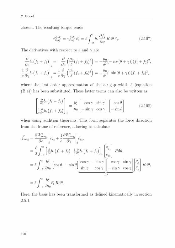
2 Model
chosen. The resulting torque reads
�τ (M)mag = τ (M)
mag �ez = �
∫ π
−πbr∂f2∂φ
Rdθ �ez. (2.107)
The derivatives with respect to e and γ are
∂
∂ebr(f1 + f2
)∣∣∣∣i
=∂
∂e
(μ0δ(f1 + f2)
2)= −μ0
δ2(− cos(θ + γ))(f1 + f2)
2,
1
e
∂
∂γbr(f1 + f2
)∣∣∣∣i
=1
e
∂
∂γ
(μ0δ(f1 + f2)
2)= −μ0
δ2( sin(θ + γ))(f1 + f2)
2,
where the first order approximation of the air-gap width δ (equation
(B.4)) has been substituted. These latter terms can also be written as⎡⎣ ∂
∂ebr(f1 + f2
)1e∂∂γbr(f1 + f2
)⎤⎦i
=b2rμ0
[cos γ sin γ
− sin γ cos γ
][cos θ
− sin θ
](2.108)
when using addition theorems. This form separates the force direction
from the frame of reference, allowing to calculate
�fmag =∂W ∗
mag
∂e
∣∣∣∣i
�ex3 +1
e
∂W ∗mag
∂γ
∣∣∣∣i
�ey3,
=�
2
∫ π
−π
[∂∂ebr(f1 + f2
)1e∂∂γbr(f1 + f2
)]i
[�ex3�ey3
]Rdθ,
= �
∫ π
−π
b2r2μ0
[cos θ − sin θ
][cos γ − sin γ
sin γ cos γ
][cos γ sin γ
− sin γ cos γ
]︸ ︷︷ ︸
=I
[�ex
�ey
]Rdθ,
= �
∫ π
−π
b2r2μ0
�erRdθ.
Here, the basis has been transformed as defined kinematically in section
2.5.1.
120
2.6 Electromechanical Coupling
The flux linkage is calculated directly from the co-energy, reading
λk =∂W ∗
mag
∂ik
∣∣∣∣x
=∂
∂ik
∣∣∣∣x
(�
2
∫ π
−πbr(f1 + f2)Rdθ +
∫ F b,1
F b,0
Φ�b dF b
), (2.109)
where k = 1, ..., ne. The detailed derivative of these integral expressions
will not be given here. Within the next paragraph it will be shown, that
this expression is equivalent to (2.102c), which is much simpler to evalua-
te.
Summarising the results, the analytical electromechanical coupling reads
�τ (M)mag = �
∫ π
−πbr∂f2∂φ
�ez Rdθ, (2.110a)
�fmag = �
∫ π
−π
b2r2μ0
�erRdθ, (2.110b)
λk =∂
∂ik
∣∣∣∣x
(�
2
∫ π
−pibr(f1 + f2)Rdθ +
∫ F b,1
F b,0
Φb dF b
), (2.110c)
where k = 1, ..., ne.
2.6.3 Equivalence of the Classical and Analytical Coupling
In order to show the equivalence between the coupling for the classical
and analytical approaches, the equivalence of each equation in (2.102) and
(2.110) will be shown individually. The proof is first carried out without
the consideration of effects due to slots. The consequences of the slotting
extension are discussed at the end of this section.
121
2 Model
Equivalence of the torque expressions
When equations (2.102a) and (2.110a) are supposed to yield the same
result, the condition
∂f2∂θ
=∂f2∂φ
(2.111)
has to be fulfilled. To show this, f2 can be expressed as a Fourier series,
accounting for the coordinate change θ2 = θ + φ due to the rotor motion
f2 =∞∑
ν=−∞f (2)2νe−jν(θ+φ). (2.112)
Here, f (2)2ν
is the ν-th harmonic of f2 with respect to the rotor fixed frame
of reference (superscript (2)). From this relation it can be seen that the
condition is always fulfilled as it does not matter whether the derivative
is carried out with respect to θ, or φ.
Equivalence of the force expressions
Equations (2.102b) and (2.110b) are already equal, therefore, no further
calculations are necessary.
Equivalence of the flux linkage expressions
Showing the equivalence for the flux linkage is a little more elaborate,
if the solid parts are taken into account. Therefore, this task will be tack-
led in two steps: at first, the equivalence will be shown when the influence
of the solid domains can be neglected. After that a general proof will be
given.
If the MMF drop along the solid parts can be neglected the second part
in equation (2.110c) can be omitted. Thus, the energy derivative can be
122
2.6 Electromechanical Coupling
written as
λk =∂
∂ik
∣∣∣∣x
�
2
∫ π
−π
μ0δ(f1 + f2)
2Rdθ, k = 1, ..., ne. (2.113)
In this equation, the only quantities depending on the currents are the
boundary MMF f1 and f2 and by virtue of relation (2.89), it becomes
λk = �
∫ π
−πbr
(∂F�
a1
∂ikG1 +
∂F�a2
∂ikG2
)Rdθ. (2.114)
Due to the linear magnetic behaviour the terms ∂F�a1
∂ikand ∂F�
a2
∂ikhave to
be constant matrices. In fact, their entries are equal to the number of
turns Nj of the coil (j = 1, ..., ncl), through which the current ik flows.
The position of each entry in the matrix indicates, which air-gap MMF
component is caused by which current. Using this information and writing
the matrix products∂F�
a,i
∂ikGi as sums over all non-vanishing entries yields
λk =
ncl∑j=1
Nj�
∫ π
−πbrGj Rdθ, (2.115)
where Gj is the component of either G1, or G2, belonging to the j-th
matrix entry. The only difference between this latter expression and the
classical definition (2.102c) of the flux linkage is, that in (2.102c), the
circumferential integration is carried out from one coil end to the other,
while in the derived analytical equation the integration is taken over the
whole circumference and the integrand is multiplied with the geometry
function Gj. However, taking a closer look at the geometry functions (as
depicted for example in figure 2.28 c)) reveals, that their sum is equal to
one in the passive zones between the coil ends and zero elsewhere. The-
refore, expressions (2.102c) and (2.115) are identical.
For this first proof, the influence of the solid parts has been neglected.
Reconsidering equation (2.110c) shows that an equivalent approach for
the general case would not be constructive as on the one side the air-gap
123
2 Model
MMF F a now is a non-linear function of the currents and as on the other
side the relation between branch fluxes Φb branch MMF F b and the cur-
rents i is determined by an implicit function.
Alternatively, the proof can be conducted using a more general metho-
dology. As it has been shown in equations (2.88) and (2.101), both parts
of the co-energy in (2.110c) have been derived from the general formula
(2.38). Taking the latter one as a starting point the equivalence can be
shown when arguing reversely to the common derivation of the magnetic
energy, as shown for example by Stratton [131, p. 118-125].
Starting from (2.38) and using the magnetic vector potential �a, as defined
in (2.75), the magnetic co-energy can be written in terms of
W ∗mag =
∫V∞
[∫ �h
�h0
�b · d�h]dV =
∫Ω
[∫ �h
�h0
(∇× �a) · d�h]dV. (2.116)
Where the volume V∞ has been reduced to the machine domain Ω, ass-
uming that the magnetic field vanishes outside the machine. Exploiting
the vector identity
(∇× �a) · d�h = �a · (∇× d�h)︸ ︷︷ ︸d�j
−∇ · (d�h× �a), (2.117)
identifying the current density differential d�j and using Stoke’s theorem
yields
W ∗mag =
∫Ω
[∫ �j
�j0
�a · d�j]dV −
∮Γ
�a× d�h, (2.118)
where Γ is the machine outer boundary. The second term in this equation
vanishes, if the boundary condition �a∣∣Γ= �0 is set27.
27This condition can be interpreted as a magnetic insulation and is consistent to the assumption ofvanishing field strength outside the machine.
124
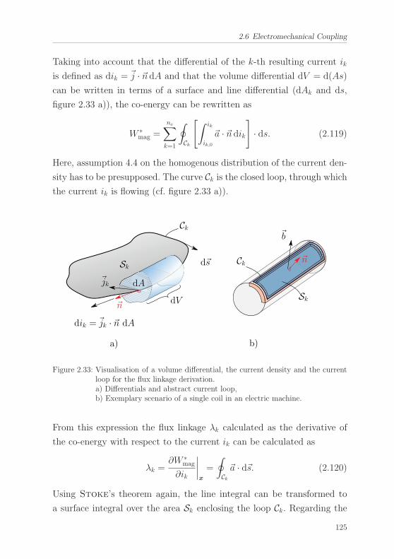
2.6 Electromechanical Coupling
Taking into account that the differential of the k-th resulting current ik
is defined as dik = �j · �n dA and that the volume differential dV = d(As)
can be written in terms of a surface and line differential (dAk and ds,
figure 2.33 a)), the co-energy can be rewritten as
W ∗mag =
ne∑k=1
∮Ck
[∫ ik
ik,0
�a · �n dik]· ds. (2.119)
Here, assumption 4.4 on the homogenous distribution of the current den-
sity has to be presupposed. The curve Ck is the closed loop, through which
the current ik is flowing (cf. figure 2.33 a)).
a) b)
dV�n
d�s
dA
dik = �jk · �n dA
Ck
Sk Ck
Sk�jk
�n
�b
Figure 2.33: Visualisation of a volume differential, the current density and the currentloop for the flux linkage derivation.a) Differentials and abstract current loop,b) Exemplary scenario of a single coil in an electric machine.
From this expression the flux linkage λk calculated as the derivative of
the co-energy with respect to the current ik can be calculated as
λk =∂W ∗
mag
∂ik
∣∣∣∣x
=
∮Ck�a · d�s. (2.120)
Using Stoke’s theorem again, the line integral can be transformed to
a surface integral over the area Sk enclosing the loop Ck. Regarding the
125
2 Model
definition of the vector potential in (2.75), the flux linkage becomes
λk =
∫Sk
(∇× �a) · �n dA =
∫Sk
�b · �n dA. (2.121)
Figure 2.33 b) depicts such a scenario, where the current flows through
just one coil with one turn. If it passes mk coils having Ni turns (i =
1, ...,mk), their contributions to the flux linkage have to be summarised
and weighted with Ni, such that the final statement is
λk =
ncl∑i=1
Ni�
∫ θcr,i
θcl,i
brRdθ. (2.122)
Here, θcl,i and θcr,i are the circumferential boundaries of the i-th coil, as
defined earlier.
Finally, comparing equations (2.102c) and (2.122) shows that also the
flux linkages are equivalent for the classical and analytical approach. This
completes the proof and shows two things: first, the theoretical framework
is mathematically consistent as it has been derived in two different axio-
matic ways. And second, the electromechanical coupling stated in this
section is energetically consistent as all coupling variables can be derived
from a single functional.
Considering the effect of slots
In section 2.5.1, the field solution has been modified in order to account
for effects caused by slots adjacent to the air-gap. It has been shown, that
modulating the radial component of the flux density also means modula-
ting the boundary MMF f1 and f2. This modulation has no effect on the
calculation of the flux linkage and magnetic forces. Therefore, the proof
of equivalence as stated above is not changed for these variables.
126
2.6 Electromechanical Coupling
However, the picture changes when considering the magnetic torque. In
this case the boundary MMF has been modified according to
f2 = S2f2. (2.123)
Under these circumstances condition (2.111) is still valid and the value of
the torque matches to the one calculated via finite element simulations.
As stated in section 2.5.1, the boundary condition at the outer border of
the air-gap is no longer fulfilled. In view of this fact, the torque cannot
be evaluated at the air-gap outer boundary for the formulae given here.
However, it would be possible to derive an alternative approximation for
the magnetic potential, such that the outer boundary condition would be
met, while the inner would be violated. Therefore, the only precaution
to be taken is to be aware, what boundary to use for the torque evaluation.
Interestingly, using the energy gradient to evaluate the torque always
leads to the correct result. This is due to the fact that the energy functio-
nal (or its gradient) does not depend on the tangential field component,
but solely on the boundary MMF. It is unsurprising that a vast majority
of publications applying analytical approximations with slotting effects
considered use an energy functional to calculate the torque (cf. [33],[50,
p. 102],[132],[133]).
127
2 Model
2.6.4 Conclusions
To end the section on the electromechanical coupling, the following con-
clusions are drawn
Conclusions 5: Electromechanical Coupling
1. The most important result derived from the magnetic field pro-blem is the electromechanical coupling in terms of torque, forceand flux linkage. These quantities have been derived both forclassical and analytical dynamics. At the end of this sectionit has been shown, that both these formulations are equiva-lent. Therefore, the coupling stated within this work is bothmathematically and energetically consistent.
2. Based on the considerations concerning the electromechanicalcoupling it turned out that when modulating the radial fluxdensity to account for slotting effects, the boundary MMF alsomust be modulated to provide for a valid magnetic torqueexpression.
3. As the slotting modulation approach always violates oneof the two air-gap boundary conditions, it has to be carefullyconsidered, which boundary to choose for the torque calcula-tion when using the Maxwell stress tensor. In contrast tothat, using an energy gradient for the torque calculation al-ways leads to valid results.
128
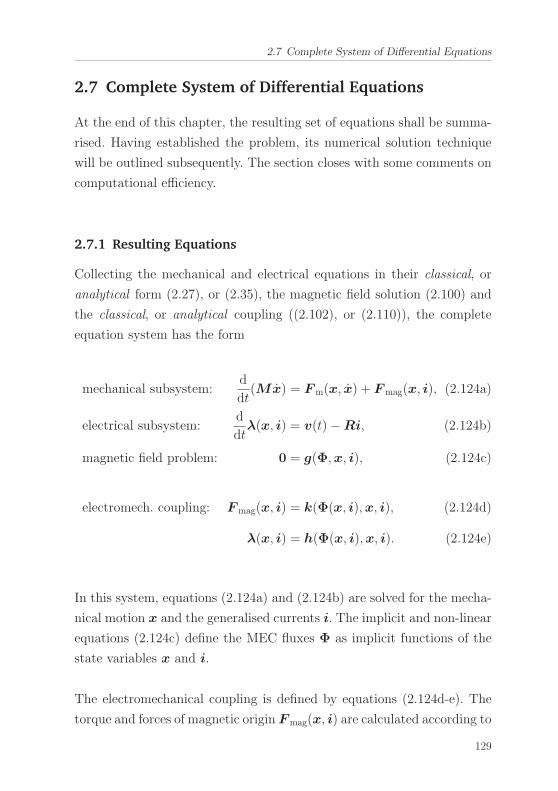
2.7 Complete System of Differential Equations
2.7 Complete System of Differential Equations
At the end of this chapter, the resulting set of equations shall be summa-
rised. Having established the problem, its numerical solution technique
will be outlined subsequently. The section closes with some comments on
computational efficiency.
2.7.1 Resulting Equations
Collecting the mechanical and electrical equations in their classical, or
analytical form (2.27), or (2.35), the magnetic field solution (2.100) and
the classical, or analytical coupling ((2.102), or (2.110)), the complete
equation system has the form
mechanical subsystem:d
dt(Mx) = Fm(x, x) + Fmag(x, i), (2.124a)
electrical subsystem:d
dtλ(x, i) = v(t)−Ri, (2.124b)
magnetic field problem: 0 = g(Φ,x, i), (2.124c)
electromech. coupling: Fmag(x, i) = k(Φ(x, i),x, i), (2.124d)
λ(x, i) = h(Φ(x, i),x, i). (2.124e)
In this system, equations (2.124a) and (2.124b) are solved for the mecha-
nical motion x and the generalised currents i. The implicit and non-linear
equations (2.124c) define the MEC fluxes Φ as implicit functions of the
state variables x and i.
The electromechanical coupling is defined by equations (2.124d-e). The
torque and forces of magnetic origin Fmag(x, i) are calculated according to
129
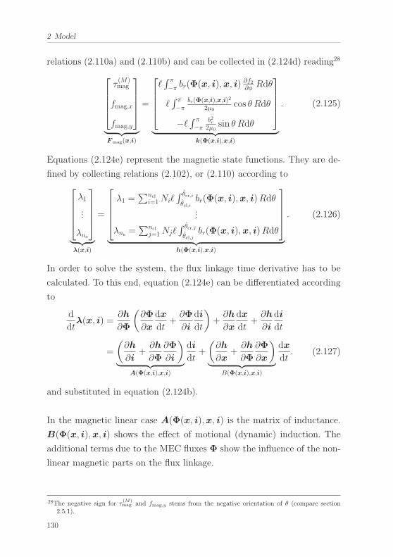
2 Model
relations (2.110a) and (2.110b) and can be collected in (2.124d) reading28⎡⎢⎢⎢⎣τ(M)mag
fmag,x
fmag,y
⎤⎥⎥⎥⎦
︸ ︷︷ ︸Fmag(x,i)
=
⎡⎢⎢⎢⎣�∫ π−π br(Φ(x, i),x, i) ∂f2∂φ Rdθ
�∫ π−π
br(Φ(x,i),x,i)2
2μ0cos θ Rdθ
−� ∫ π−π b2r2μ0
sin θ Rdθ
⎤⎥⎥⎥⎦
︸ ︷︷ ︸k(Φ(x,i),x,i)
. (2.125)
Equations (2.124e) represent the magnetic state functions. They are de-
fined by collecting relations (2.102), or (2.110) according to⎡⎢⎢⎢⎣λ1...
λne
⎤⎥⎥⎥⎦
︸ ︷︷ ︸λ(x,i)
=
⎡⎢⎢⎢⎣λ1 =
∑ncl
i=1Ni�∫ θcr,iθcl,i
br(Φ(x, i),x, i)Rdθ...
λne=∑ncl
j=1Nj�∫ θcr,jθcl,j
br(Φ(x, i),x, i)Rdθ
⎤⎥⎥⎥⎦
︸ ︷︷ ︸h(Φ(x,i),x,i)
. (2.126)
In order to solve the system, the flux linkage time derivative has to be
calculated. To this end, equation (2.124e) can be differentiated according
to
d
dtλ(x, i) =
∂h
∂Φ
(∂Φ
∂x
dx
dt+∂Φ
∂i
di
dt
)+∂h
∂x
dx
dt+∂h
∂i
di
dt
=
(∂h
∂i+∂h
∂Φ
∂Φ
∂i
)︸ ︷︷ ︸
A(Φ(x,i),x,i)
di
dt+
(∂h
∂x+∂h
∂Φ
∂Φ
∂x
)︸ ︷︷ ︸
B(Φ(x,i),x,i)
dx
dt. (2.127)
and substituted in equation (2.124b).
In the magnetic linear case A(Φ(x, i),x, i) is the matrix of inductance.
B(Φ(x, i),x, i) shows the effect of motional (dynamic) induction. The
additional terms due to the MEC fluxes Φ show the influence of the non-
linear magnetic parts on the flux linkage.
28The negative sign for τ(M)mag and fmag,y stems from the negative orientation of θ (compare section
2.5.1).
130
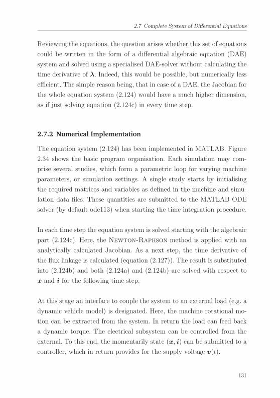
2.7 Complete System of Differential Equations
Reviewing the equations, the question arises whether this set of equations
could be written in the form of a differential algebraic equation (DAE)
system and solved using a specialised DAE-solver without calculating the
time derivative of λ. Indeed, this would be possible, but numerically less
efficient. The simple reason being, that in case of a DAE, the Jacobian for
the whole equation system (2.124) would have a much higher dimension,
as if just solving equation (2.124c) in every time step.
2.7.2 Numerical Implementation
The equation system (2.124) has been implemented in MATLAB. Figure
2.34 shows the basic program organisation. Each simulation may com-
prise several studies, which form a parametric loop for varying machine
parameters, or simulation settings. A single study starts by initialising
the required matrices and variables as defined in the machine and simu-
lation data files. These quantities are submitted to the MATLAB ODE
solver (by default ode113) when starting the time integration procedure.
In each time step the equation system is solved starting with the algebraic
part (2.124c). Here, the Newton-Raphson method is applied with an
analytically calculated Jacobian. As a next step, the time derivative of
the flux linkage is calculated (equation (2.127)). The result is substituted
into (2.124b) and both (2.124a) and (2.124b) are solved with respect to
x and i for the following time step.
At this stage an interface to couple the system to an external load (e.g. a
dynamic vehicle model) is designated. Here, the machine rotational mo-
tion can be extracted from the system. In return the load can feed back
a dynamic torque. The electrical subsystem can be controlled from the
external. To this end, the momentarily state (x, i) can be submitted to a
controller, which in return provides for the supply voltage v(t).
131
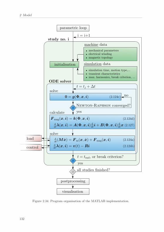
2 Model
d
dtλ(x, i) = v(t)−Ri
d
dt(Mx) = Fm(x, x) + Fmag(x, i)
solve
0 = g(Φ,x, i)
Newton-Raphson converged?
solveno
yes
yes
t = tend, or break criterion?
t = tj +Δt
ODE solver
initialisation
study no. i
machine data
simulation data
all studies finished?
postprocessing
visualisation
parametric loop
i = i+1
control
load
electrical windingmagnetic topology
mechanical parameters
simulation time, motion type,...transient characteristicsmax. harmonics, break criterion, ...
calculate
d
dtλ(x, i) = A(Φ,x, i) ddti+B(Φ,x, i) d
dtx
(2.124c)
(2.127)
(2.124a)
(2.124b)
Fmag(x, i) = k(Φ,x, i) (2.124d)
Figure 2.34: Program organisation of the MATLAB implementation.
132
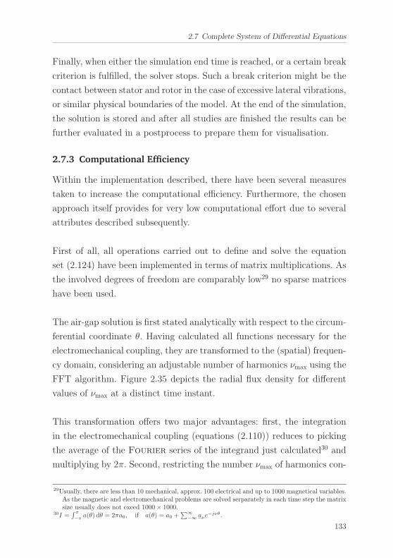
2.7 Complete System of Differential Equations
Finally, when either the simulation end time is reached, or a certain break
criterion is fulfilled, the solver stops. Such a break criterion might be the
contact between stator and rotor in the case of excessive lateral vibrations,
or similar physical boundaries of the model. At the end of the simulation,
the solution is stored and after all studies are finished the results can be
further evaluated in a postprocess to prepare them for visualisation.
2.7.3 Computational Efficiency
Within the implementation described, there have been several measures
taken to increase the computational efficiency. Furthermore, the chosen
approach itself provides for very low computational effort due to several
attributes described subsequently.
First of all, all operations carried out to define and solve the equation
set (2.124) have been implemented in terms of matrix multiplications. As
the involved degrees of freedom are comparably low29 no sparse matrices
have been used.
The air-gap solution is first stated analytically with respect to the circum-
ferential coordinate θ. Having calculated all functions necessary for the
electromechanical coupling, they are transformed to the (spatial) frequen-
cy domain, considering an adjustable number of harmonics νmax using the
FFT algorithm. Figure 2.35 depicts the radial flux density for different
values of νmax at a distinct time instant.
This transformation offers two major advantages: first, the integration
in the electromechanical coupling (equations (2.110)) reduces to picking
the average of the Fourier series of the integrand just calculated30 and
multiplying by 2π. Second, restricting the number νmax of harmonics con-
29Usually, there are less than 10 mechanical, approx. 100 electrical and up to 1000 magnetical variables.As the magnetic and electromechanical problems are solved serparately in each time step the matrixsize usually does not exeed 1000× 1000.
30I =∫ π
−πa(θ) dθ = 2πa0, if a(θ) = a0 +
∑∞−∞ aνe
−jνθ.
133
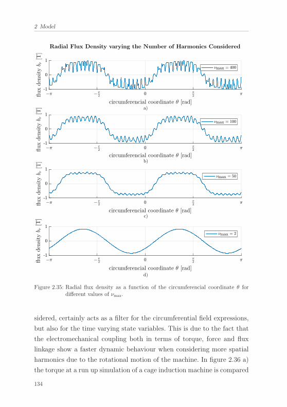
2 Model
a)
b)
c)
d)
Radial Flux Density varying the Number of Harmonics Considered
circumferencial coordinate θ [rad]
circumferencial coordinate θ [rad]
circumferencial coordinate θ [rad]
circumferencial coordinate θ [rad]
fluxdensityb r
[T]
fluxdensityb r
[T]
fluxdensityb r
[T]
fluxdensityb r
[T]
Figure 2.35: Radial flux density as a function of the circumferencial coordinate θ fordifferent values of νmax.
sidered, certainly acts as a filter for the circumferential field expressions,
but also for the time varying state variables. This is due to the fact that
the electromechanical coupling both in terms of torque, force and flux
linkage show a faster dynamic behaviour when considering more spatial
harmonics due to the rotational motion of the machine. In figure 2.36 a)
the torque at a run up simulation of a cage induction machine is compared
134
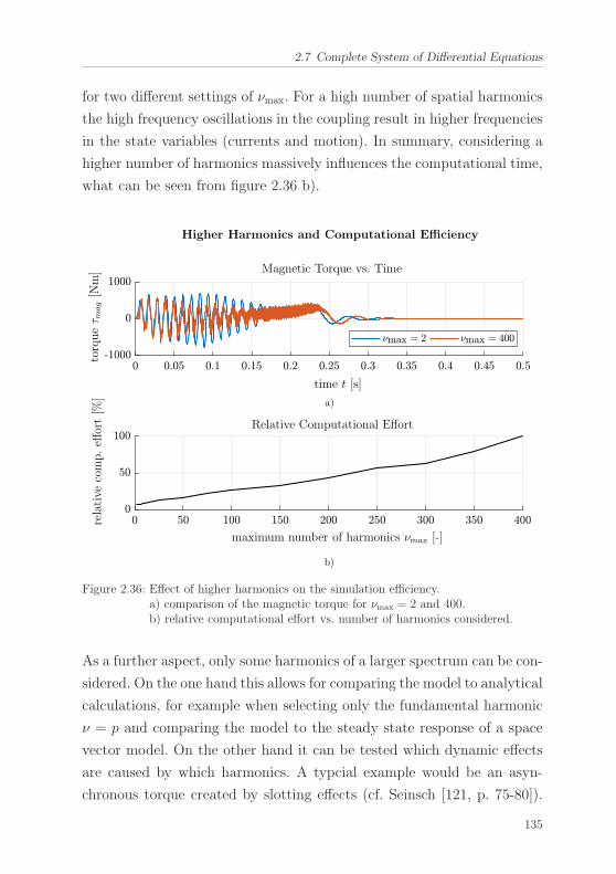
2.7 Complete System of Differential Equations
for two different settings of νmax. For a high number of spatial harmonics
the high frequency oscillations in the coupling result in higher frequencies
in the state variables (currents and motion). In summary, considering a
higher number of harmonics massively influences the computational time,
what can be seen from figure 2.36 b).
a)
b)
maximum number of harmonics νmax [-]
relative
comp.eff
ort[%
]
Relative Computational Effort
Magnetic Torque vs. Time
time t [s]
torqueτ m
ag[N
m]
Higher Harmonics and Computational Efficiency
Figure 2.36: Effect of higher harmonics on the simulation efficiency.a) comparison of the magnetic torque for νmax = 2 and 400.b) relative computational effort vs. number of harmonics considered.
As a further aspect, only some harmonics of a larger spectrum can be con-
sidered. On the one hand this allows for comparing the model to analytical
calculations, for example when selecting only the fundamental harmonic
ν = p and comparing the model to the steady state response of a space
vector model. On the other hand it can be tested which dynamic effects
are caused by which harmonics. A typcial example would be an asyn-
chronous torque created by slotting effects (cf. Seinsch [121, p. 75-80]).
135
2 Model
They could only be observed when inluding the harmonics concerned and
could be isolated, if only the fundamental and this harmonic would be
considered.
To increase the efficiency of the Newton-Raphson algorithm, the Ja-
cobian has been calculated analytically. Figure 2.37 shows the iterations
needed in the run-up simulation shown in figure 2.36 for νmax = 400 har-
monics. To initialise the algorithm in the next time step, the previous
result is utilised. With this, the average number of iterations is 1.1 and
the maximum is 3. The highest numbers of iterations occur, if the magne-
tic field harmonics are strongly changing in amplitude. This is the case
at the end of the acceleration process (compare figure 2.36 a)).
As a last point, the magnetic field problem in the solid domain (equation
(2.124c)) can be deactivated, if saturation effects are of no interest. In
this case, the implemented model is equivalent to the air-gap permeance
methods [19, 20, 23, 33].
time t [s]
no.
ofiterationsN
[-]
Iterations needed for a Run-up Simulation
Figure 2.37: Iterations needed for the Newton-Raphson algorithm at different timesteps. The average number of iterations is 1.1, the maximum number is 3.
136
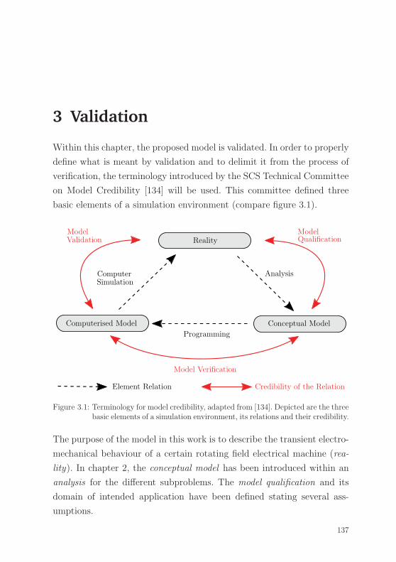
3 Validation
Within this chapter, the proposed model is validated. In order to properly
define what is meant by validation and to delimit it from the process of
verification, the terminology introduced by the SCS Technical Committee
on Model Credibility [134] will be used. This committee defined three
basic elements of a simulation environment (compare figure 3.1).
Reality
Conceptual ModelComputerised Model
Analysis
Programming
ComputerSimulation
Model Model
Model Verification
Validation Qualification
Element Relation Credibility of the Relation
Figure 3.1: Terminology for model credibility, adapted from [134]. Depicted are the threebasic elements of a simulation environment, its relations and their credibility.
The purpose of the model in this work is to describe the transient electro-
mechanical behaviour of a certain rotating field electrical machine (rea-
lity). In chapter 2, the conceptual model has been introduced within an
analysis for the different subproblems. The model qualification and its
domain of intended application have been defined stating several ass-
umptions.
137
3 Validation
In section 2.7, the computerised model has been introduced and some
aspects of the numerical MATLAB implementation have been discussed.
A model verification has been carried out throughout the implementati-
on process. To this end, different test cases have been designed and the
formulae have been checked against numerical computation.
Finally, this section will assess whether the computerised model agrees
with reality within its domain of applicability and to the extend of a cer-
tain range of accuracy.
In general, not all aspects of the model will be validated. For example,
measuring the actual rotor orbit within an electrical machine at opera-
tion would be a challenging task. The literature on this subject is rare1,
although some attempts have been made (as for instance by Zarko et al.
[127]). For this reason, only magnetic forces due to a certain rotor motion
are validated here. Some remarks on future validation experiments are
given in chapter 5.
In all validation simulations, the variables to be compared are first visuali-
sed for a qualitative comparison. After that, a quantitative error measure
is defined and the range of accuracy of the proposed model is assessed.
Assuming, that the result of the proposed model comprises n values
ai (i = 1, ..., n) and that the reference leads to corresponding results bi
(cf. figure 3.2), the relative error between the proposed model and the
reference reads
Ei = ai − bibnom.
, i = 1, ..., n,
where bnom. is some nominal value of the reference result. Intuitively, itwould make sense to simply chose bnom. = bi. However, if the values (ai, bi)
1This statement should not be confused with the state of literature on machine monitoring in gene-ral. There is a lot of literature on monitoring the shaft motion at the bearings. However, if suchmeasurements where to be used for validation, an accurate bearing model would have to be included.
138
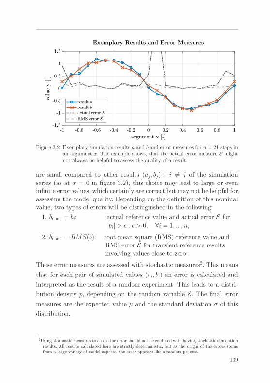
Figure 3.2: Exemplary simulation results a and b and error measures for n = 21 steps inan argument x. The example shows, that the actual error measure E mightnot always be helpful to assess the quality of a result.
are small compared to other results (aj, bj) : i �= j of the simulationseries (as at x = 0 in figure 3.2), this choice may lead to large or eveninfinite error values, which certainly are correct but may not be helpful forassessing the model quality. Depending on the definition of this nominalvalue, two types of errors will be distinguished in the following:
1. bnom. = bi: actual reference value and actual error E for|bi| > ε : ε > 0, ∀i = 1, ..., n,
2. bnom. = RMS(b): root mean square (RMS) reference value andRMS error E for transient reference resultsinvolving values close to zero.
These error measures are assessed with stochastic measures2. This means
that for each pair of simulated values (ai, bi) an error is calculated and
interpreted as the result of a random experiment. This leads to a distri-
bution density p, depending on the random variable E . The final error
measures are the expected value μ and the standard deviation σ of this
distribution.
2Using stochastic measures to assess the error should not be confused with having stochastic simulationresults. All results calculated here are strictly deterministic, but as the origin of the errors stemsfrom a large variety of model aspects, the error appears like a random process.
139
3 Validation
The validation in this chapter comprises two different machine types: a ca-ge induction motor and an interior permanent magnet synchronous motor(IPMSM) with v-shaped permanent magnets. The validation simulationscover the following two aspects:
1. Static Validation: Comparison of the magnetic field, the torqueand the force with finite element simulationsand measurements for prescribed currents andmotion.
2. Dynamic Validation: Dynamic comparison of currents and motionwith a space vector model.
In the following, the main characteristics of both machines are described
first, followed by a presentation and discussion of the validation simu-
lations. At the end, some conclusions are drawn. More details on the
machines and their models are given in appendix D.
140
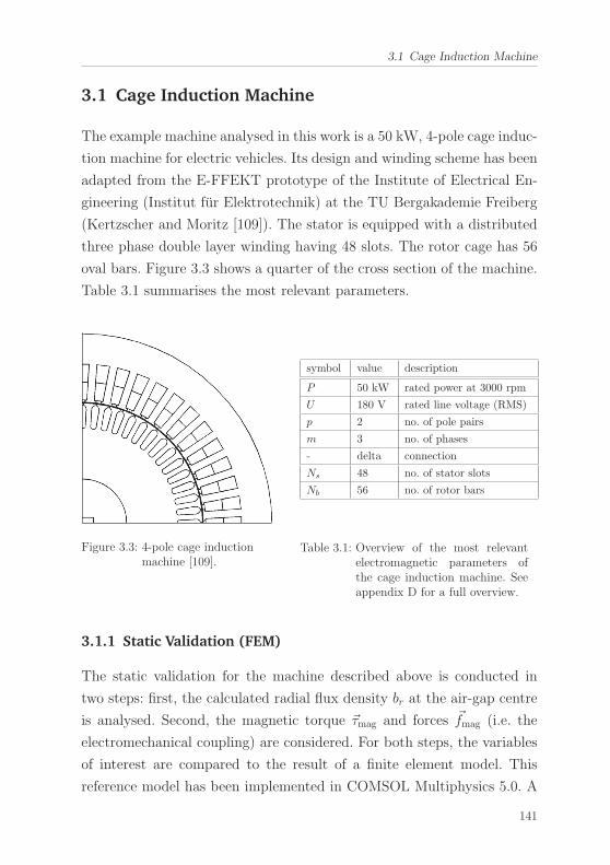
3.1 Cage Induction Machine
3.1 Cage Induction Machine
The example machine analysed in this work is a 50 kW, 4-pole cage induc-
tion machine for electric vehicles. Its design and winding scheme has been
adapted from the E-FFEKT prototype of the Institute of Electrical En-
gineering (Institut fur Elektrotechnik) at the TU Bergakademie Freiberg
(Kertzscher and Moritz [109]). The stator is equipped with a distributed
three phase double layer winding having 48 slots. The rotor cage has 56
oval bars. Figure 3.3 shows a quarter of the cross section of the machine.
Table 3.1 summarises the most relevant parameters.
Figure 3.3: 4-pole cage inductionmachine [109].
symbol value description
P 50 kW rated power at 3000 rpm
U 180 V rated line voltage (RMS)
p 2 no. of pole pairs
m 3 no. of phases
- delta connection
Ns 48 no. of stator slots
Nb 56 no. of rotor bars
Table 3.1: Overview of the most relevantelectromagnetic parameters ofthe cage induction machine. Seeappendix D for a full overview.
3.1.1 Static Validation (FEM)
The static validation for the machine described above is conducted in
two steps: first, the calculated radial flux density br at the air-gap centre
is analysed. Second, the magnetic torque �τmag and forces �fmag (i.e. the
electromechanical coupling) are considered. For both steps, the variables
of interest are compared to the result of a finite element model. This
reference model has been implemented in COMSOL Multiphysics 5.0. A
141
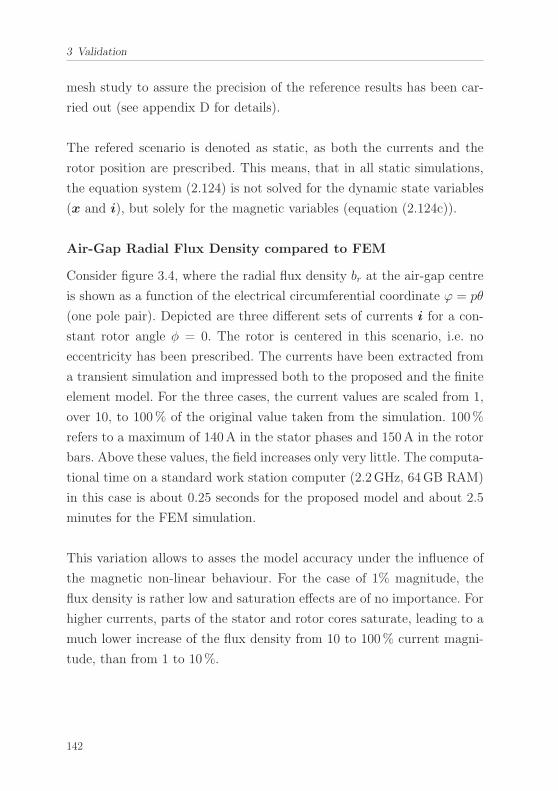
3 Validation
mesh study to assure the precision of the reference results has been car-
ried out (see appendix D for details).
The refered scenario is denoted as static, as both the currents and the
rotor position are prescribed. This means, that in all static simulations,
the equation system (2.124) is not solved for the dynamic state variables
(x and i), but solely for the magnetic variables (equation (2.124c)).
Air-Gap Radial Flux Density compared to FEM
Consider figure 3.4, where the radial flux density br at the air-gap centre
is shown as a function of the electrical circumferential coordinate ϕ = pθ
(one pole pair). Depicted are three different sets of currents i for a con-
stant rotor angle φ = 0. The rotor is centered in this scenario, i.e. no
eccentricity has been prescribed. The currents have been extracted from
a transient simulation and impressed both to the proposed and the finite
element model. For the three cases, the current values are scaled from 1,
over 10, to 100% of the original value taken from the simulation. 100%
refers to a maximum of 140A in the stator phases and 150A in the rotor
bars. Above these values, the field increases only very little. The computa-
tional time on a standard work station computer (2.2GHz, 64GB RAM)
in this case is about 0.25 seconds for the proposed model and about 2.5
minutes for the FEM simulation.
This variation allows to asses the model accuracy under the influence of
the magnetic non-linear behaviour. For the case of 1% magnitude, the
flux density is rather low and saturation effects are of no importance. For
higher currents, parts of the stator and rotor cores saturate, leading to a
much lower increase of the flux density from 10 to 100% current magni-
tude, than from 1 to 10%.
142
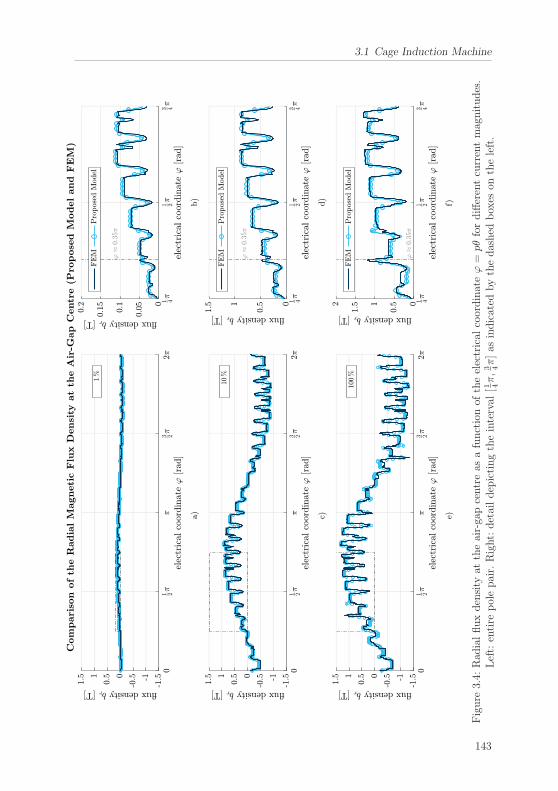
3.1 Cage Induction Machine
Figure
3.4:
Rad
ialfluxdensity
attheair-gapcentreas
afunctionof
theelectrical
coordinateϕ=pθ
fordifferentcurrentmagnitudes.
Left:entire
polepair.Right:detaildepictingtheinterval
[1 4π,3 4π]as
indicated
bythedashed
boxes
ontheleft.
143
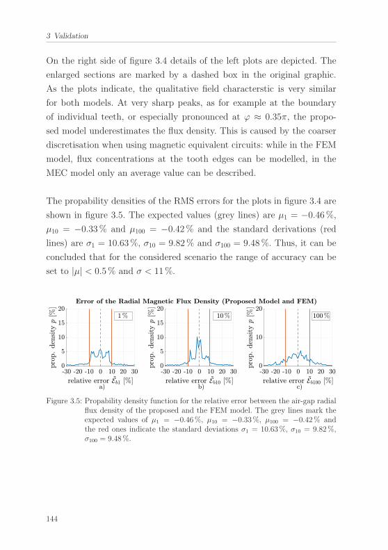
3 Validation
On the right side of figure 3.4 details of the left plots are depicted. The
enlarged sections are marked by a dashed box in the original graphic.
As the plots indicate, the qualitative field characterstic is very similar
for both models. At very sharp peaks, as for example at the boundary
of individual teeth, or especially pronounced at ϕ ≈ 0.35π, the propo-
sed model underestimates the flux density. This is caused by the coarser
discretisation when using magnetic equivalent circuits: while in the FEM
model, flux concentrations at the tooth edges can be modelled, in the
MEC model only an average value can be described.
The propability densities of the RMS errors for the plots in figure 3.4 are
shown in figure 3.5. The expected values (grey lines) are μ1 = −0.46%,
μ10 = −0.33% and μ100 = −0.42% and the standard derivations (red
lines) are σ1 = 10.63%, σ10 = 9.82% and σ100 = 9.48%. Thus, it can be
concluded that for the considered scenario the range of accuracy can be
set to |μ| < 0.5% and σ < 11%.
Figure 3.5: Propability density function for the relative error between the air-gap radialflux density of the proposed and the FEM model. The grey lines mark theexpected values of μ1 = −0.46%, μ10 = −0.33%, μ100 = −0.42% andthe red ones indicate the standard deviations σ1 = 10.63%, σ10 = 9.82%,σ100 = 9.48%.
144
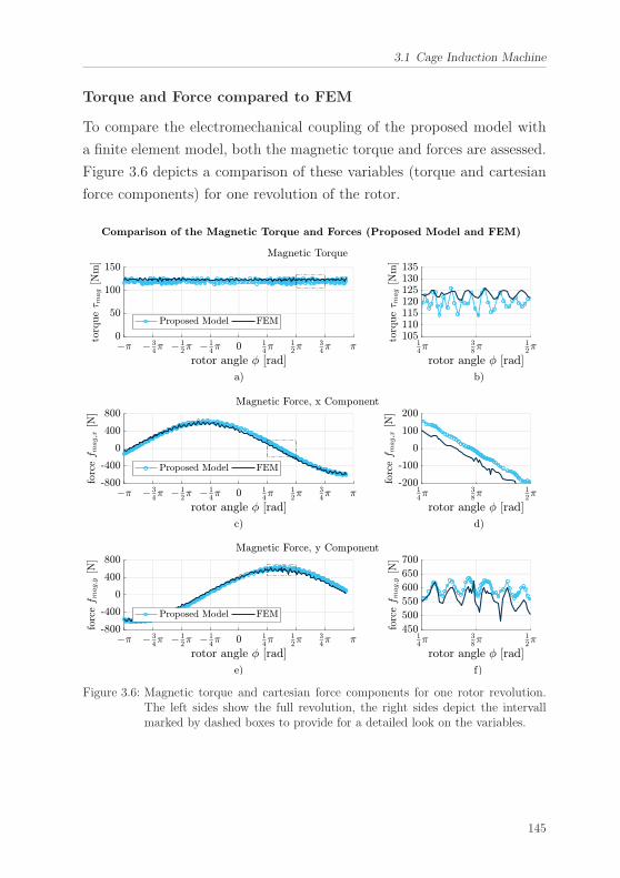
3.1 Cage Induction Machine
Torque and Force compared to FEM
To compare the electromechanical coupling of the proposed model with
a finite element model, both the magnetic torque and forces are assessed.
Figure 3.6 depicts a comparison of these variables (torque and cartesian
force components) for one revolution of the rotor.
Figure 3.6: Magnetic torque and cartesian force components for one rotor revolution.The left sides show the full revolution, the right sides depict the intervallmarked by dashed boxes to provide for a detailed look on the variables.
145
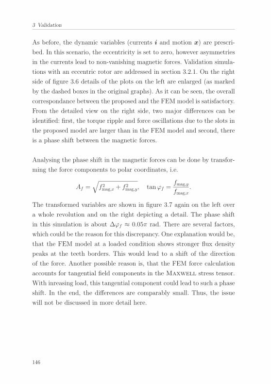
3 Validation
As before, the dynamic variables (currents i and motion x) are prescri-
bed. In this scenario, the eccentricity is set to zero, however asymmetries
in the currents lead to non-vanishing magnetic forces. Validation simula-
tions with an eccentric rotor are addressed in section 3.2.1. On the right
side of figure 3.6 details of the plots on the left are enlarged (as marked
by the dashed boxes in the original graphs). As it can be seen, the overall
correspondance between the proposed and the FEM model is satisfactory.
From the detailed view on the right side, two major differences can be
identified: first, the torque ripple and force oscillations due to the slots in
the proposed model are larger than in the FEM model and second, there
is a phase shift between the magnetic forces.
Analysing the phase shift in the magnetic forces can be done by transfor-
ming the force components to polar coordinates, i.e.
Af =√f 2mag,x + f 2mag,y, tanϕf =
fmag,y
fmag,x.
The transformed variables are shown in figure 3.7 again on the left over
a whole revolution and on the right depicting a detail. The phase shift
in this simulation is about Δϕf ≈ 0.05π rad. There are several factors,
which could be the reason for this discrepancy. One explanation would be,
that the FEM model at a loaded condition shows stronger flux density
peaks at the teeth borders. This would lead to a shift of the direction
of the force. Another possible reason is, that the FEM force calculation
accounts for tangential field components in the Maxwell stress tensor.
With inreasing load, this tangential component could lead to such a phase
shift. In the end, the differences are comparably small. Thus, the issue
will not be discussed in more detail here.
146
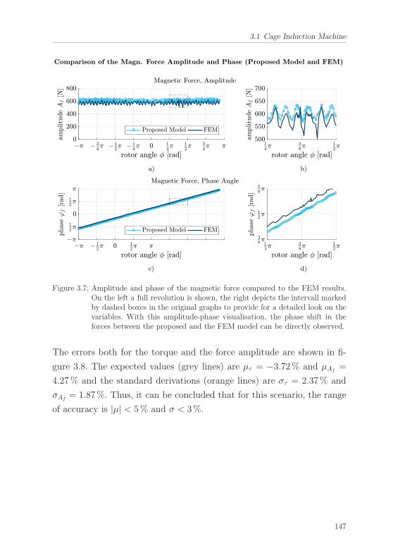
3.1 Cage Induction Machine
Figure 3.7: Amplitude and phase of the magnetic force compared to the FEM results.On the left a full revolution is shown, the right depicts the intervall markedby dashed boxes in the original graphs to provide for a detailed look on thevariables. With this amplitude-phase visualisation, the phase shift in theforces between the proposed and the FEM model can be directly observed.
The errors both for the torque and the force amplitude are shown in fi-
gure 3.8. The expected values (grey lines) are μτ = −3.72% and μAf=
4.27% and the standard derivations (orange lines) are στ = 2.37% and
σAf= 1.87%. Thus, it can be concluded that for this scenario, the range
of accuracy is |μ| < 5% and σ < 3%.
147
3 Validation
Figure 3.8: Error propability density of the magnetic torque and force amplitude. Theexpected values (marked in grey) of the errors are μτ = −3.72% and μAf
=4.27%. The standard deviations (red lines) are στ = 2.37% and σAf
=1.87%.
3.1.2 Dynamic Validation (Space Vector)
In this next validation step, the whole equation system (2.7) is solved and
compared to a space vector model. The approach for the cage induction
machine is adapted from Munoz and Lipo [135]. This particular type of
model allows to match the machine parameters to the exact attributes
of a cage induction machine under transient conditions and includes a
transformation to calculate each individual mesh/bar current. The mo-
del parameters and system equations are also summarised in appendix D.
Solving the whole equation system means that the state variables (the
currents i and motion x) are calculated dynamically. As in the section
above, the eccentricity is set to zero3. In order to validate the dynamic
equation system the following scenario is analysed: The machine is sup-
plied by a prescribed and perfectly sinusoidal three phase voltage of 180V
(RMS) and a frequency of 100 Hz. Thus, the machine is accelerated from
0 to 3000 rpm and runs in idle state afterwards. After one second, a load
torque is applied and increased linearly in time by 500 Nm/s. This pro-
3Common space vector models cannot account for eccentricity.
148
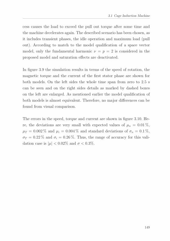
3.1 Cage Induction Machine
cess causes the load to exceed the pull out torque after some time and
the machine decelerates again. The described scenario has been chosen, as
it includes transient phases, the idle operation and maximum load (pull
out). According to match to the model qualification of a space vector
model, only the fundamental harmonic ν = p = 2 is considered in the
proposed model and saturation effects are deactivated.
In figure 3.9 the simulation results in terms of the speed of rotation, the
magnetic torque and the current of the first stator phase are shown for
both models. On the left sides the whole time span from zero to 2.5 s
can be seen and on the right sides details as marked by dashed boxes
on the left are enlarged. As mentioned earlier the model qualification of
both models is almost equivalent. Therefore, no major differences can be
found from visual comparison.
The errors in the speed, torque and current are shown in figure 3.10. He-
re, the deviations are very small with expected values of μn = 0.01%,
μT = 0.002% and μi = 0.004% and standard deviations of σn = 0.1%,
σT = 0.22% and σi = 0.26%. Thus, the range of accuracy for this vali-
dation case is |μ| < 0.02% and σ < 0.3%.
149
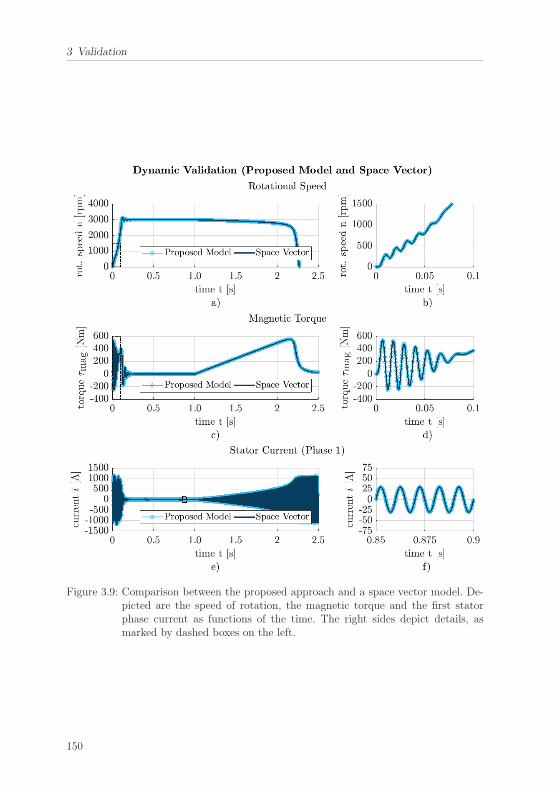
3 Validation
Figure 3.9: Comparison between the proposed approach and a space vector model. De-picted are the speed of rotation, the magnetic torque and the first statorphase current as functions of the time. The right sides depict details, asmarked by dashed boxes on the left.
150
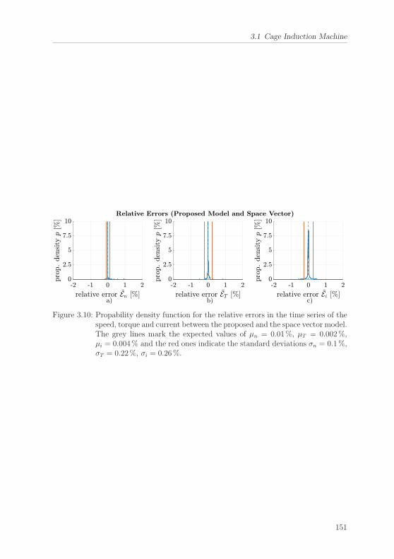
3.1 Cage Induction Machine
Figure 3.10: Propability density function for the relative errors in the time series of thespeed, torque and current between the proposed and the space vector model.The grey lines mark the expected values of μn = 0.01%, μT = 0.002%,μi = 0.004% and the red ones indicate the standard deviations σn = 0.1%,σT = 0.22%, σi = 0.26%.
151
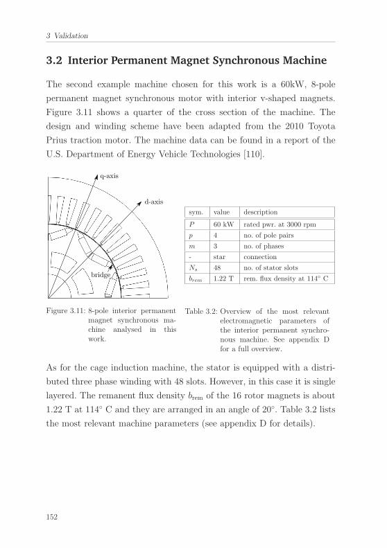
3 Validation
3.2 Interior Permanent Magnet Synchronous Machine
The second example machine chosen for this work is a 60kW, 8-pole
permanent magnet synchronous motor with interior v-shaped magnets.
Figure 3.11 shows a quarter of the cross section of the machine. The
design and winding scheme have been adapted from the 2010 Toyota
Prius traction motor. The machine data can be found in a report of the
U.S. Department of Energy Vehicle Technologies [110].
q-axis
d-axis
bridge
Figure 3.11: 8-pole interior permanentmagnet synchronous ma-chine analysed in thiswork.
sym. value description
P 60 kW rated pwr. at 3000 rpm
p 4 no. of pole pairs
m 3 no. of phases
- star connection
Ns 48 no. of stator slots
brem 1.22 T rem. flux density at 114◦ C
Table 3.2: Overview of the most relevantelectromagnetic parameters ofthe interior permanent synchro-nous machine. See appendix Dfor a full overview.
As for the cage induction machine, the stator is equipped with a distri-
buted three phase winding with 48 slots. However, in this case it is single
layered. The remanent flux density brem of the 16 rotor magnets is about
1.22 T at 114◦ C and they are arranged in an angle of 20◦. Table 3.2 lists
the most relevant machine parameters (see appendix D for details).
152
3.2 Interior Permanent Magnet Synchronous Machine
3.2.1 Static Validation (FEM)
As for the cage induction machine, the static validation comprises two
steps: first, the magnetic flux density br at the air-gap centre of the propo-
sed model is compared to the results of a finite element simulation. After
that, the magnetic torque �τmag and forces �fmag, as well as the induced vol-
tage vind are compared to measurements and finite element simulations.
Please remember that the term static validation implies that both the
currents, as well as the rotor position are prescribed. This means, that
the equation system (2.124) is not solved for the dynamic state variables
(x and i), but solely for the magnetic variables (equation (2.124c)).
Air-Gap Radial Flux Density compared to FEM
In figure 3.12 the radial magnetic flux density br at the air-gap centre is
shown as a function of the electrical circumferential angle ϕ = pθ (one
pole pair). The left side of each row shows an overview and the right side
depicts a detail (as marked by a dashed box on the left). Each row shows
a different scenario: in the upper one, the stator current is set to zero so
that the field solely caused by the permanent magnets can be validated.
In the middle, a current phasor of 50A is applied4 to the stator winding
oriented towards the d-axis (cf. figure 3.11). Finally, the last row shows
a setting with the same 50A current phasor but oriented towards the
q-axis.
4This means an amplitude of 50A projected to the direction of interest. The term d-axis refers to thedirect orientation of the permanent magnet field and q-axis to the direction between two magneticpoles (quadrature axis).
153
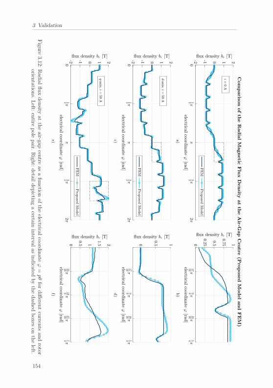
3 Validation
Figu
re3.12:
Rad
ialfluxdensity
attheair-gap
centre
asafunction
oftheelectrical
coord
inate
ϕ=pθ
fordifferen
tcurren
tsan
drotor
orientation
s.Left:
entire
pole
pair.
Righ
t:detail
depictin
gacertain
interval
asindicated
bythedash
edboxes
ontheleft.
154
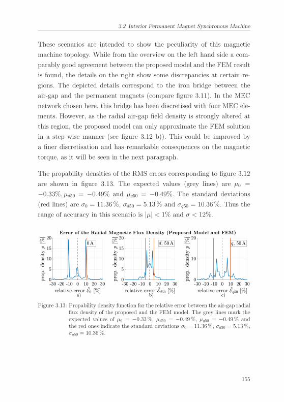
3.2 Interior Permanent Magnet Synchronous Machine
These scenarios are intended to show the peculiarity of this magnetic
machine topology. While from the overview on the left hand side a com-
parably good agreement between the proposed model and the FEM result
is found, the details on the right show some discrepancies at certain re-
gions. The depicted details correspond to the iron bridge between the
air-gap and the permanent magnets (compare figure 3.11). In the MEC
network chosen here, this bridge has been discretised with four MEC ele-
ments. However, as the radial air-gap field density is strongly altered at
this region, the proposed model can only approximate the FEM solution
in a step wise manner (see figure 3.12 b)). This could be improved by
a finer discretisation and has remarkable consequences on the magnetic
torque, as it will be seen in the next paragraph.
The propability densities of the RMS errors corresponding to figure 3.12
are shown in figure 3.13. The expected values (grey lines) are μ0 =
−0.33%, μd50 = −0.49% and μq50 = −0.49%. The standard deviations
(red lines) are σ0 = 11.36%, σd50 = 5.13% and σq50 = 10.36%. Thus the
range of accuracy in this scenario is |μ| < 1% and σ < 12%.
Figure 3.13: Propability density function for the relative error between the air-gap radialflux density of the proposed and the FEM model. The grey lines mark theexpected values of μ0 = −0.33%, μd50 = −0.49%, μq50 = −0.49% andthe red ones indicate the standard deviations σ0 = 11.36%, σd50 = 5.13%,σq50 = 10.36%.
155
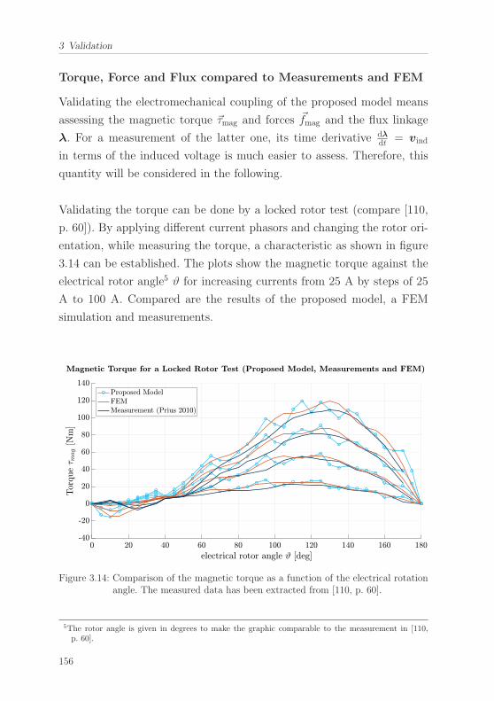
3 Validation
Torque, Force and Flux compared to Measurements and FEM
Validating the electromechanical coupling of the proposed model means
assessing the magnetic torque �τmag and forces �fmag and the flux linkage
λ. For a measurement of the latter one, its time derivative dλdt = vind
in terms of the induced voltage is much easier to assess. Therefore, this
quantity will be considered in the following.
Validating the torque can be done by a locked rotor test (compare [110,
p. 60]). By applying different current phasors and changing the rotor ori-
entation, while measuring the torque, a characteristic as shown in figure
3.14 can be established. The plots show the magnetic torque against the
electrical rotor angle5 ϑ for increasing currents from 25 A by steps of 25
A to 100 A. Compared are the results of the proposed model, a FEM
simulation and measurements.
Figure 3.14: Comparison of the magnetic torque as a function of the electrical rotationangle. The measured data has been extracted from [110, p. 60].
5The rotor angle is given in degrees to make the graphic comparable to the measurement in [110,p. 60].
156
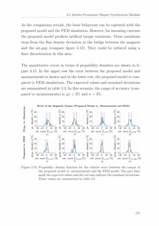
3.2 Interior Permanent Magnet Synchronous Machine
As the comparison reveals, the basic behaviour can be captured with the
proposed model and the FEM simulation. However, for inreasing currents
the proposed model predicts artifical torque variations. These variations
stem from the flux density deviation at the bridge between the magnets
and the air-gap (compare figure 3.12). They could be reduced using a
finer discretisation in this area.
The quantitative errors in terms of propability densities are shown in fi-
gure 3.15. In the upper row the error between the proposed model and
measurements is shown and in the lower row, the proposed model is com-
pared to FEM simulations. The expected values and standard deviations
are summarised in table 3.3. In this scenario, the range of accuracy (com-
pared to measurements) is |μ| < 3% and σ < 4%.
Figure 3.15: Propability density function for the relative error between the torque ofthe proposed model vs. measurements and the FEM model. The grey linesmark the expected values and the red ones indicate the standard deviations.These values are summarised in table 3.3.
157
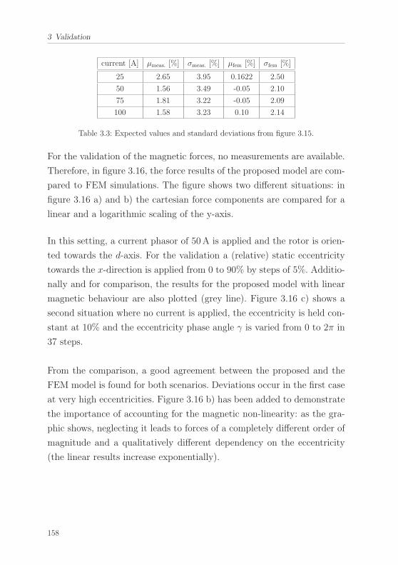
3 Validation
current [A] μmeas. [%] σmeas. [%] μfem [%] σfem [%]
25 2.65 3.95 0.1622 2.50
50 1.56 3.49 -0.05 2.10
75 1.81 3.22 -0.05 2.09
100 1.58 3.23 0.10 2.14
Table 3.3: Expected values and standard deviations from figure 3.15.
For the validation of the magnetic forces, no measurements are available.
Therefore, in figure 3.16, the force results of the proposed model are com-
pared to FEM simulations. The figure shows two different situations: in
figure 3.16 a) and b) the cartesian force components are compared for a
linear and a logarithmic scaling of the y-axis.
In this setting, a current phasor of 50A is applied and the rotor is orien-
ted towards the d-axis. For the validation a (relative) static eccentricity
towards the x-direction is applied from 0 to 90% by steps of 5%. Additio-
nally and for comparison, the results for the proposed model with linear
magnetic behaviour are also plotted (grey line). Figure 3.16 c) shows a
second situation where no current is applied, the eccentricity is held con-
stant at 10% and the eccentricity phase angle γ is varied from 0 to 2π in
37 steps.
From the comparison, a good agreement between the proposed and the
FEM model is found for both scenarios. Deviations occur in the first case
at very high eccentricities. Figure 3.16 b) has been added to demonstrate
the importance of accounting for the magnetic non-linearity: as the gra-
phic shows, neglecting it leads to forces of a completely different order of
magnitude and a qualitatively different dependency on the eccentricity
(the linear results increase exponentially).
158
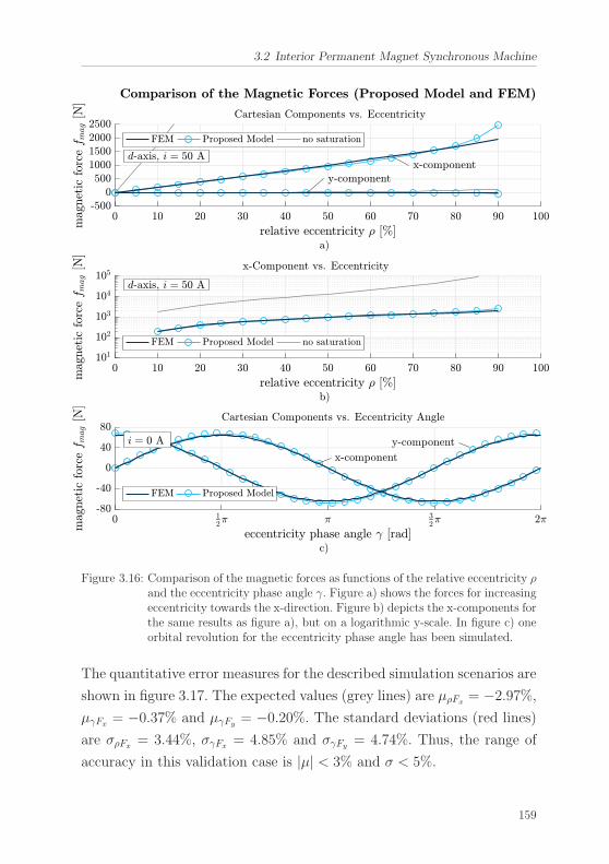
3.2 Interior Permanent Magnet Synchronous Machine
Figure 3.16: Comparison of the magnetic forces as functions of the relative eccentricity ρand the eccentricity phase angle γ. Figure a) shows the forces for increasingeccentricity towards the x-direction. Figure b) depicts the x-components forthe same results as figure a), but on a logarithmic y-scale. In figure c) oneorbital revolution for the eccentricity phase angle has been simulated.
The quantitative error measures for the described simulation scenarios are
shown in figure 3.17. The expected values (grey lines) are μρFx= −2.97%,
μγFx= −0.37% and μγFy
= −0.20%. The standard deviations (red lines)
are σρFx= 3.44%, σγFx
= 4.85% and σγFy= 4.74%. Thus, the range of
accuracy in this validation case is |μ| < 3% and σ < 5%.
159
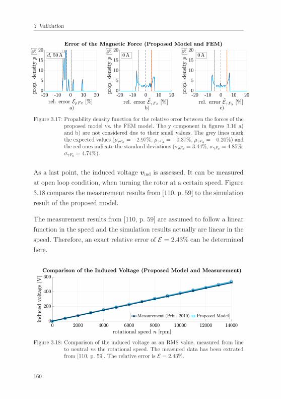
3 Validation
Figure 3.17: Propability density function for the relative error between the forces of theproposed model vs. the FEM model. The y component in figures 3.16 a)and b) are not considered due to their small values. The grey lines markthe expected values (μρFx = −2.97%, μγFx = −0.37%, μγFy = −0.20%) andthe red ones indicate the standard deviations (σρFx = 3.44%, σγFx = 4.85%,σγFy = 4.74%).
As a last point, the induced voltage vind is assessed. It can be measured
at open loop condition, when turning the rotor at a certain speed. Figure
3.18 compares the measurement results from [110, p. 59] to the simulation
result of the proposed model.
The measurement results from [110, p. 59] are assumed to follow a linear
function in the speed and the simulation results actually are linear in the
speed. Therefore, an exact relative error of E = 2.43% can be determined
here.
Figure 3.18: Comparison of the induced voltage as an RMS value, measured from lineto neutral vs the rotational speed. The measured data has been extratedfrom [110, p. 59]. The relative error is E = 2.43%.
160
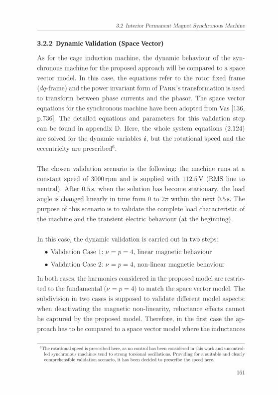
3.2 Interior Permanent Magnet Synchronous Machine
3.2.2 Dynamic Validation (Space Vector)
As for the cage induction machine, the dynamic behaviour of the syn-
chronous machine for the proposed approach will be compared to a space
vector model. In this case, the equations refer to the rotor fixed frame
(dq-frame) and the power invariant form of Park’s transformation is used
to transform between phase currents and the phasor. The space vector
equations for the synchronous machine have been adopted from Vas [136,
p.736]. The detailed equations and parameters for this validation step
can be found in appendix D. Here, the whole system equations (2.124)
are solved for the dynamic variables i, but the rotational speed and the
eccentricity are prescribed6.
The chosen validation scenario is the following: the machine runs at a
constant speed of 3000 rpm and is supplied with 112.5V (RMS line to
neutral). After 0.5 s, when the solution has become stationary, the load
angle is changed linearly in time from 0 to 2π within the next 0.5 s. The
purpose of this scenario is to validate the complete load characteristic of
the machine and the transient electric behaviour (at the beginning).
In this case, the dynamic validation is carried out in two steps:
• Validation Case 1: ν = p = 4, linear magnetic behaviour
• Validation Case 2: ν = p = 4, non-linear magnetic behaviour
In both cases, the harmonics considered in the proposed model are restric-
ted to the fundamental (ν = p = 4) to match the space vector model. The
subdivision in two cases is supposed to validate different model aspects:
when deactivating the magnetic non-linearity, reluctance effects cannot
be captured by the proposed model. Therefore, in the first case the ap-
proach has to be compared to a space vector model where the inductances
6The rotational speed is prescribed here, as no control has been considered in this work and uncontrol-led synchronous machines tend to strong torsional oscillations. Providing for a suitable and clearlycomprehensible validation scenario, it has been decided to prescribe the speed here.
161
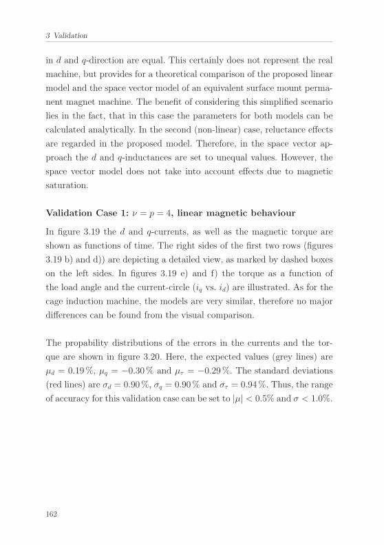
3 Validation
in d and q-direction are equal. This certainly does not represent the real
machine, but provides for a theoretical comparison of the proposed linear
model and the space vector model of an equivalent surface mount perma-
nent magnet machine. The benefit of considering this simplified scenario
lies in the fact, that in this case the parameters for both models can be
calculated analytically. In the second (non-linear) case, reluctance effects
are regarded in the proposed model. Therefore, in the space vector ap-
proach the d and q-inductances are set to unequal values. However, the
space vector model does not take into account effects due to magnetic
saturation.
Validation Case 1: ν = p = 4, linear magnetic behaviour
In figure 3.19 the d and q-currents, as well as the magnetic torque are
shown as functions of time. The right sides of the first two rows (figures
3.19 b) and d)) are depicting a detailed view, as marked by dashed boxes
on the left sides. In figures 3.19 e) and f) the torque as a function of
the load angle and the current-circle (iq vs. id) are illustrated. As for the
cage induction machine, the models are very similar, therefore no major
differences can be found from the visual comparison.
The propability distributions of the errors in the currents and the tor-
que are shown in figure 3.20. Here, the expected values (grey lines) are
μd = 0.19%, μq = −0.30% and μτ = −0.29%. The standard deviations
(red lines) are σd = 0.90%, σq = 0.90% and στ = 0.94%. Thus, the range
of accuracy for this validation case can be set to |μ| < 0.5% and σ < 1.0%.
162
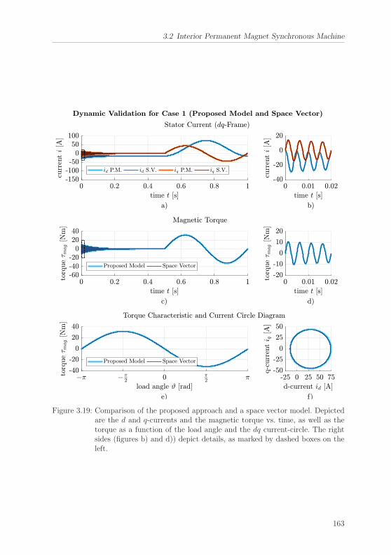
3.2 Interior Permanent Magnet Synchronous Machine
Figure 3.19: Comparison of the proposed approach and a space vector model. Depictedare the d and q-currents and the magnetic torque vs. time, as well as thetorque as a function of the load angle and the dq current-circle. The rightsides (figures b) and d)) depict details, as marked by dashed boxes on theleft.
163
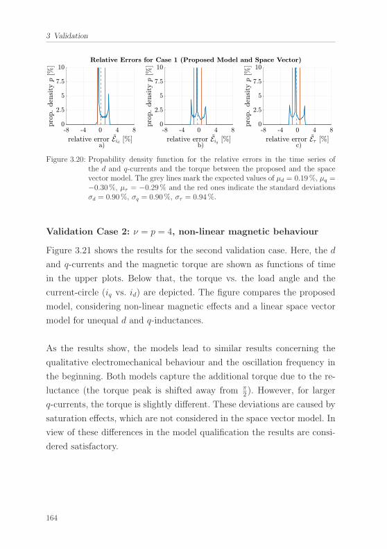
3 Validation
Figure 3.20: Propability density function for the relative errors in the time series ofthe d and q-currents and the torque between the proposed and the spacevector model. The grey lines mark the expected values of μd = 0.19%, μq =−0.30%, μτ = −0.29% and the red ones indicate the standard deviationsσd = 0.90%, σq = 0.90%, στ = 0.94%.
Validation Case 2: ν = p = 4, non-linear magnetic behaviour
Figure 3.21 shows the results for the second validation case. Here, the d
and q-currents and the magnetic torque are shown as functions of time
in the upper plots. Below that, the torque vs. the load angle and the
current-circle (iq vs. id) are depicted. The figure compares the proposed
model, considering non-linear magnetic effects and a linear space vector
model for unequal d and q-inductances.
As the results show, the models lead to similar results concerning the
qualitative electromechanical behaviour and the oscillation frequency in
the beginning. Both models capture the additional torque due to the re-
luctance (the torque peak is shifted away from π2 ). However, for larger
q-currents, the torque is slightly different. These deviations are caused by
saturation effects, which are not considered in the space vector model. In
view of these differences in the model qualification the results are consi-
dered satisfactory.
164
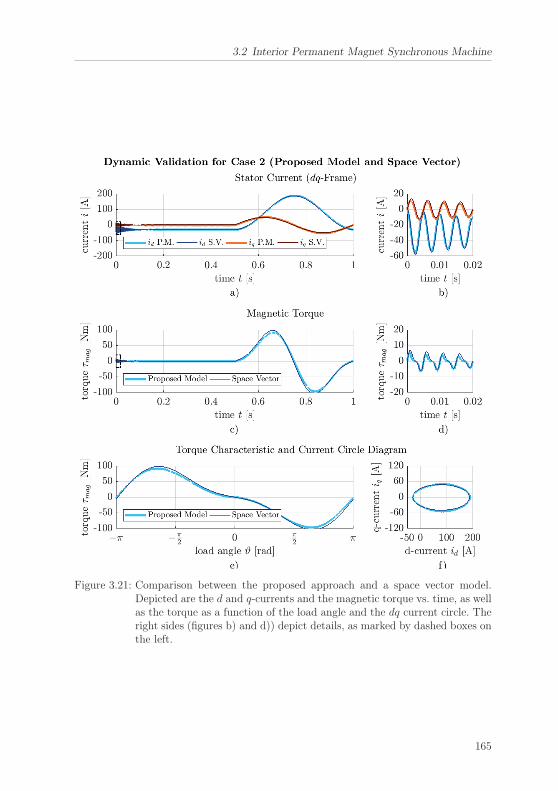
3.2 Interior Permanent Magnet Synchronous Machine
Figure 3.21: Comparison between the proposed approach and a space vector model.Depicted are the d and q-currents and the magnetic torque vs. time, as wellas the torque as a function of the load angle and the dq current circle. Theright sides (figures b) and d)) depict details, as marked by dashed boxes onthe left.
165
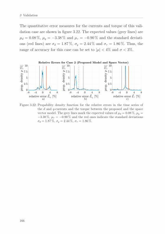
3 Validation
The quantitative error measures for the currents and torque of this vali-
dation case are shown in figure 3.22. The expected values (grey lines) are
μd = 0.08%, μq = −3.38% and μτ = −0.90% and the standard deviati-
ons (red lines) are σd = 1.87%, σq = 2.44% and στ = 1.86%. Thus, the
range of accuracy for this case can be set to |μ| < 4% and σ < 3%.
Figure 3.22: Propability density function for the relative errors in the time series ofthe d and q-currents and the torque between the proposed and the spacevector model. The grey lines mark the expected values of μd = 0.08%, μq =−3.38%, μτ = −0.90% and the red ones indicate the standard deviationsσd = 1.87%, σq = 2.44%, στ = 1.86%.
166
3.3 Conclusions
3.3 Conclusions
Conclusions 6: Validation
1. The proposed model has been validated using the definitionsintroduced by the SCS Technical Committee on Model Credi-bility [134].
2. The examples chosen for the comparison where a 50 kW 4-pole cage induction machine (E-FFEKT prototype [109]) anda 60 kW 8-pole interior permanent magnet synchronous motor(2010 Toyota Prius traction drive [110]).
3. An error assessment has been carried out qualitatively by vi-sualisation and quantitatively by stochastical evaluation of re-lative error measures in terms of the (empirical) error probabi-lity density p, its expected value μ and the standard deviationσ.
4. The validation for each example has been presented in twosteps: a static and a dynamic validation.
• In the static validation, the flux density at the air-gapcentre, as well as the magnetic torques, forces and fluxlinkages have been compared to measurements [110] andFEM simulations (using COMSOL Multiphysics).
• In the dynamic validation, the electrical currents and themotion calculated from the proposed model have beencompared to the results of space vector models (compare[12, pp. 1023 - 1096]).
5. The range of accuracy for the proposed model can be summa-rised as follows:
• Cage induction machine - static: |μ| < 5%, σ < 11%,
• Cage induction machine - dynamic: |μ| < 0.1%, σ < 0.3%,
• PM synchr. machine - static: |μ| < 5%, σ < 12%,
• PM synchr. machine - dynamic: |μ| < 4%, σ < 3%.
167
4 Results
Having validated the proposed model in this chapter a selection of simula-
tion studies and qualitative findings deduced from these simulations will
be discussed. The studies start by describing particular vibration pheno-
mena, which have been observed for different parameter settings. Subse-
quently, an attempt to generalise the observations is presented. Although
some fundamental findings can be derived from the simulation results it
is not intended to provide for an exhaustive rotordynamic analysis. The
main aim is to identify basic mechanisms of electromechanical resonance
and self-excitation and how they depend on the most relevant system
parameters. Throughout the chapter the same machine types as for the
validation are considered and as before they are operated with a prescri-
bed and perfectly sinusoidal supply voltage. In this chapter, the effect of
gravity is neglected, as it is not in the focus of this thesis.
The discourse is subdivided into two sections, where the first one describes
self-excited rotor oscillations of the 4-pole 50 kW cage induction machi-
ne. In the second part rotor vibrations of the 8-pole 60 kW permanent
magnet synchronous machine are analysed. This latter section consists of
two paragraphs, where the first one deals with the effect of a static dis-
placement on the dynamic orbit (compare section 2.3.1). Subsequently,
an alternative winding design involving parallel branches is introduced.
Here, self-excited oscillations due to the modified design are discussed. At
the end, the main findings are summarised by drawing some conclusions.
The critical bending speeds of both machines have been set to 16000 rpm.
This value is lower than in the real machines, but shifts the resonance clo-
se enough to the actual speed range allowing to observe the full range of
168
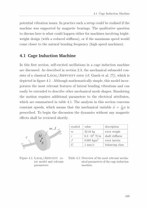
4.1 Cage Induction Machine
potential vibration issues. In practice such a setup could be realised if the
machine was supported by magnetic bearings. The qualitative question
to discuss here is what could happen either for machines involving leight-
weight design (with a reduced stiffness), or if the maximum speed would
come closer to the natural bending frequency (high speed machines).
4.1 Cage Induction Machine
In this first section, self-excited oscillations in a cage induction machine
are discussed. As described in section 2.3, the mechanical submodel con-
sists of a classical Laval/Jeffcott rotor (cf. Gasch et al. [7]), which is
depicted in figure 4.1 . Although mathematically simple, this model incor-
porates the most relevant features of lateral bending vibrations and can
easily be extended to describe other mechanical mode shapes. Simulating
the motion requires additional parameters to the electrical attributes,
which are summarised in table 4.1. The analysis in this section concerns
constant speeds, which means that the mechanical variable φ = π30n is
prescribed. To begin the discussion the dynamics without any magnetic
effects shall be reviewed shortly.
c
m, J
S
M
Figure 4.1: Laval/Jeffcott ro-tor model and relevantparameters.
symbol value description
m 22.44 kg rotor weight
c 6.3 · 107 N/m shaft stiffness
J 0.085 kgm2 rotor inertia
G 1 mm/s balancing class
Table 4.1: Overview of the most relevant mecha-nical parameters of the cage inductionmachine.
169
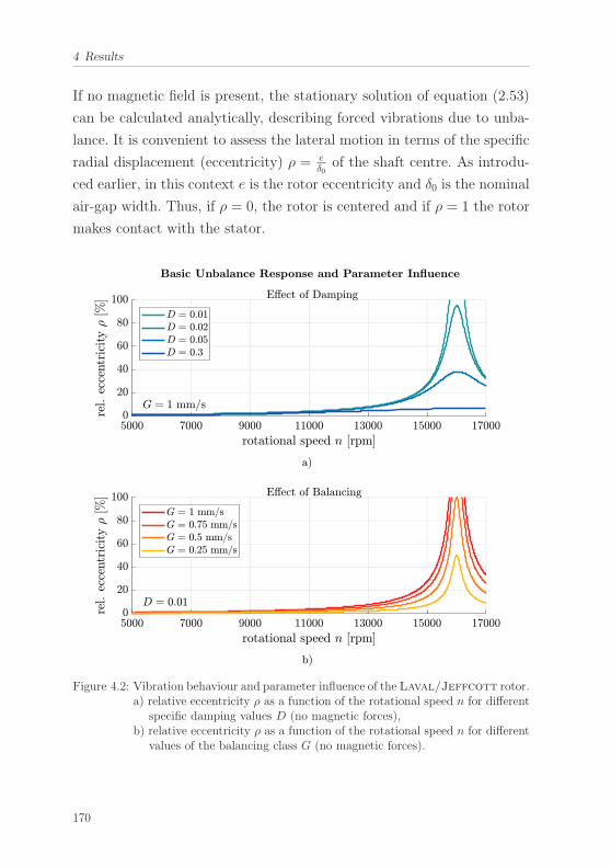
4 Results
If no magnetic field is present, the stationary solution of equation (2.53)
can be calculated analytically, describing forced vibrations due to unba-
lance. It is convenient to assess the lateral motion in terms of the specific
radial displacement (eccentricity) ρ = eδ0
of the shaft centre. As introdu-
ced earlier, in this context e is the rotor eccentricity and δ0 is the nominal
air-gap width. Thus, if ρ = 0, the rotor is centered and if ρ = 1 the rotor
makes contact with the stator.
Figure 4.2: Vibration behaviour and parameter influence of the Laval/Jeffcott rotor.a) relative eccentricity ρ as a function of the rotational speed n for different
specific damping values D (no magnetic forces),b) relative eccentricity ρ as a function of the rotational speed n for different
values of the balancing class G (no magnetic forces).
170
4.1 Cage Induction Machine
Figure 4.2 a) shows the solution in terms of ρ (in percent) as a function
of the rotational speed n for different specific damping values D = d2√cm.
Here, the resonance at 16000 rpm can be clearly identified and it beomes
apparent that for lower damping values the speed may not exceed a cer-
tain threshold in order to assure save operation.
In figure 4.2 b) the same solution for varying values of the balancing
class G are shown. In this graphic, the effect of improving the balancing
becomes evident: when decreasing G, the vibration amplitudes are signifi-
cantly reduced. These classical findings will be of importance later, when
analysing the dynamics of the system with magnetic forces.
In the following, the dynamics of the fully coupled system will be discus-
sed. To this end, the magnetic field (and forces) are no longer neglected.
The solution of the full equation system (2.124) is calculated numerically.
For the moment, the analysis is restricted to a low number of harmonics
of the air-gap field (νmax = 3), a series connection of all coil groups in
the stator winding and the neglection of saturation effects. Effects due to
model and design aspects are discussed at the end of the section.
The discourse will start with describing a single solution at a certain ro-
tational speed. Subsequently, the vibration amplitudes are analysed for
a fixed set of mechanical parameters, but as a function of the rotational
speed (as in figure 4.2). After that, the observations made in the simula-
tions are generalised for arbitrary cage induction machines. Finally, some
modelling and design aspects in terms of higher harmonics, saturation,
parallel branches and the mechanical damping are discussed.
171
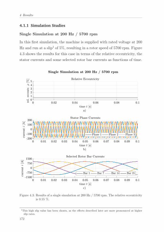
4 Results
4.1.1 Simulation Studies
Single Simulation at 200 Hz / 5700 rpm
In this first simulation, the machine is supplied with rated voltage at 200
Hz and run at a slip1 of 5%, resulting in a rotor speed of 5700 rpm. Figure
4.3 shows the results for this case in terms of the relative eccentricity, the
stator currents and some selected rotor bar currents as functions of time.
Figure 4.3: Results of a single simulation at 200 Hz / 5700 rpm. The relative eccentricityis 0.55 %.
1This high slip value has been chosen, as the effects described later are more pronounced at higherslip rates.
172
4.1 Cage Induction Machine
In this case, the specific damping has been set to D = 0 in order to ex-
clude any masking effects.
The relative eccentricity at this speed is constant at about 0.55 %, mea-
ning that the shaft centre describes a circular orbit, as it is typical for
unbalance excited oscillations. The current amplitudes are about 170 A
for the stator phases and around 1080 A for the rotor bar currents. As
expected, the stator current frequency equals 200 Hz and the rotor bar
currents oscillate at 10 Hz (the slip frequency).
When running the machine at such a comparably low speed, the electro-
mechanical coupling plays a minor role. Due to the weak coupling, the
simulation results are close to those of a decoupled system, where the
electrical part and the mechanical motion would be simulated separately.
173
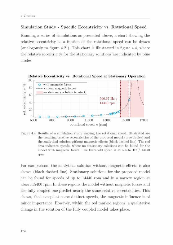
4 Results
Simulation Study - Specific Eccentricity vs. Rotational Speed
Running a series of simulations as presented above, a chart showing the
relative eccentricity as a funtion of the rotational speed can be drawn
(analogously to figure 4.2 ). This chart is illustrated in figure 4.4, where
the relative eccentricity for the stationary solutions are indicated by blue
circles.
Figure 4.4: Results of a simulation study varying the rotational speed. Illustrated arethe resulting relative eccentricities of the proposed model (blue circles) andthe analytical solution without magnetic effects (black dashed line). The redarea indicates speeds, where no stationary solutions can be found for themodel with magnetic forces. The threshold speed is at 506.67 Hz / 14440rpm.
For comparison, the analytical solution without magnetic effects is also
shown (black dashed line). Stationary solutions for the proposed model
can be found for speeds of up to 14440 rpm and in a narrow region at
about 15400 rpm. In these regions the model without magnetic forces and
the fully coupled one predict nearly the same relative eccentricities. This
shows, that except at some distinct speeds, the magnetic influence is of
minor importance. However, within the red marked regions, a qualitative
change in the solution of the fully coupled model takes place.
174
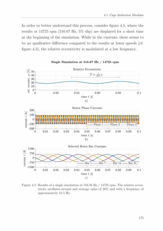
4.1 Cage Induction Machine
In order to better understand this process, consider figure 4.5, where the
results at 14725 rpm (516.67 Hz, 5% slip) are displayed for a short time
at the beginning of the simulation. While in the currents, there seems to
be no qualitative difference compared to the results at lower speeds (cf.
figure 4.3), the relative eccentricity is modulated at a low frequency.
Figure 4.5: Results of a single simulation at 516.56 Hz / 14725 rpm. The relative eccen-tricity oscillates around and average value of 20% and with a frequency ofapproximately 21.5 Hz.
175
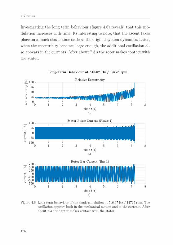
4 Results
Investigating the long term behaviour (figure 4.6) reveals, that this mo-
dulation increases with time. Its interesting to note, that the ascent takes
place on a much slower time scale as the original system dynamics. Later,
when the eccentricity becomes large enough, the additional oscillation al-
so appears in the currents. After about 7.3 s the rotor makes contact with
the stator.
Figure 4.6: Long term behaviour of the single simulation at 516.67 Hz / 14725 rpm. Theoscillation appears both in the mechanical motion and in the currents. Afterabout 7.3 s the rotor makes contact with the stator.
176
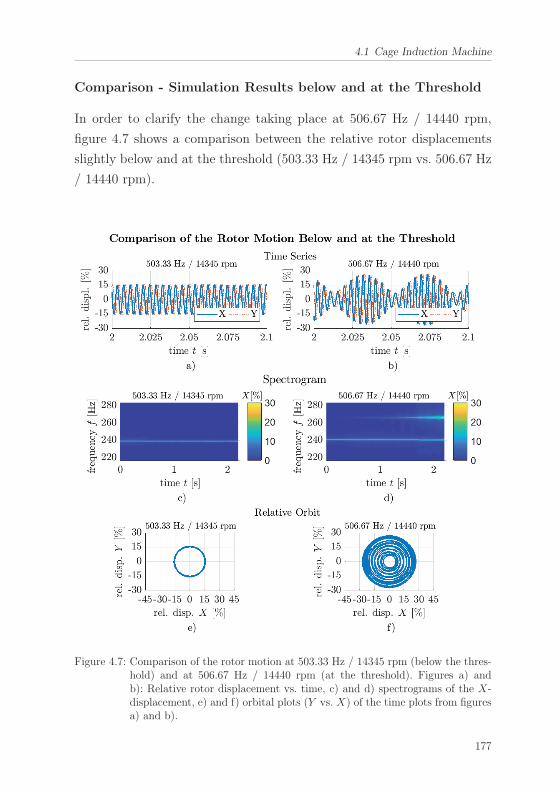
4.1 Cage Induction Machine
Comparison - Simulation Results below and at the Threshold
In order to clarify the change taking place at 506.67 Hz / 14440 rpm,
figure 4.7 shows a comparison between the relative rotor displacements
slightly below and at the threshold (503.33 Hz / 14345 rpm vs. 506.67 Hz
/ 14440 rpm).
Figure 4.7: Comparison of the rotor motion at 503.33 Hz / 14345 rpm (below the thres-hold) and at 506.67 Hz / 14440 rpm (at the threshold). Figures a) andb): Relative rotor displacement vs. time, c) and d) spectrograms of the X-displacement, e) and f) orbital plots (Y vs. X) of the time plots from figuresa) and b).
177
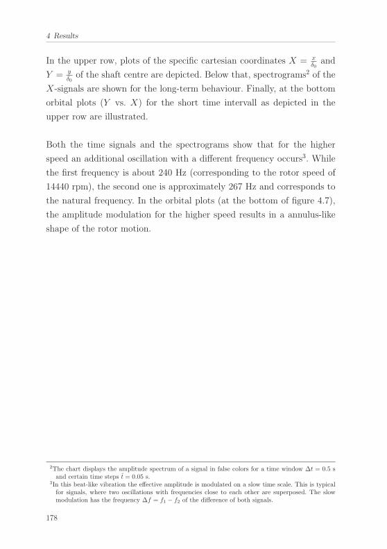
4 Results
In the upper row, plots of the specific cartesian coordinates X = xδ0
and
Y = yδ0
of the shaft centre are depicted. Below that, spectrograms2 of the
X-signals are shown for the long-term behaviour. Finally, at the bottom
orbital plots (Y vs. X) for the short time intervall as depicted in the
upper row are illustrated.
Both the time signals and the spectrograms show that for the higher
speed an additional oscillation with a different frequency occurs3. While
the first frequency is about 240 Hz (corresponding to the rotor speed of
14440 rpm), the second one is approximately 267 Hz and corresponds to
the natural frequency. In the orbital plots (at the bottom of figure 4.7),
the amplitude modulation for the higher speed results in a annulus-like
shape of the rotor motion.
2The chart displays the amplitude spectrum of a signal in false colors for a time window Δt = 0.5 sand certain time steps t = 0.05 s.
3In this beat-like vibration the effective amplitude is modulated on a slow time scale. This is typicalfor signals, where two oscillations with frequencies close to each other are superposed. The slowmodulation has the frequency Δf = f1 − f2 of the difference of both signals.
178
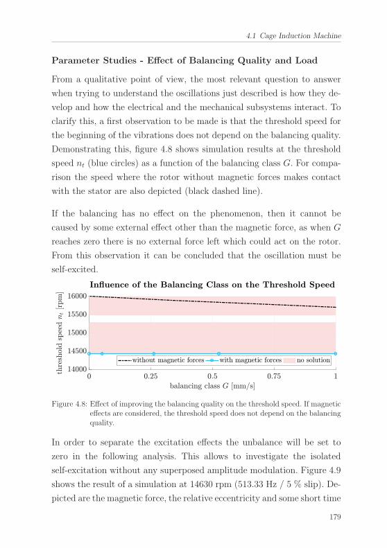
4.1 Cage Induction Machine
Parameter Studies - Effect of Balancing Quality and Load
From a qualitative point of view, the most relevant question to answer
when trying to understand the oscillations just described is how they de-
velop and how the electrical and the mechanical subsystems interact. To
clarify this, a first observation to be made is that the threshold speed for
the beginning of the vibrations does not depend on the balancing quality.
Demonstrating this, figure 4.8 shows simulation results at the threshold
speed nt (blue circles) as a function of the balancing class G. For compa-
rison the speed where the rotor without magnetic forces makes contact
with the stator are also depicted (black dashed line).
If the balancing has no effect on the phenomenon, then it cannot be
caused by some external effect other than the magnetic force, as when G
reaches zero there is no external force left which could act on the rotor.
From this observation it can be concluded that the oscillation must be
self-excited.
Figure 4.8: Effect of improving the balancing quality on the threshold speed. If magneticeffects are considered, the threshold speed does not depend on the balancingquality.
In order to separate the excitation effects the unbalance will be set to
zero in the following analysis. This allows to investigate the isolated
self-excitation without any superposed amplitude modulation. Figure 4.9
shows the result of a simulation at 14630 rpm (513.33 Hz / 5 % slip). De-
picted are the magnetic force, the relative eccentricity and some short time
179
4 Results
orbital plots. The results reveal, that as the oscillation increases especial-
ly the tangential force component grows stronger. The orbital frequency
in this scenario is always equal to the natural frequency of the underly-
ing mechanical subsystem, what is often observed for self-excitation. The
orbit is initially elliptical (figure 4.9 c)), but approaches a more and more
circular shape when the vibration becomes stronger (figures 4.9 d)-f)).
Figure 4.9: Magnetic force, relative eccentricity and orbital motion at 14360 rpm (513.33Hz / 5 % slip). a) Magnetic force components radial and tangential to theorbit, b) Relative eccentricity vs. time, b)-e) Orbital motion for 0.01 s atdifferent time instances.
The influence of the slip (i.e. the load) on the vibration gives further in-
sight to the observed phenomenon. This aspect can be analysed, when
180
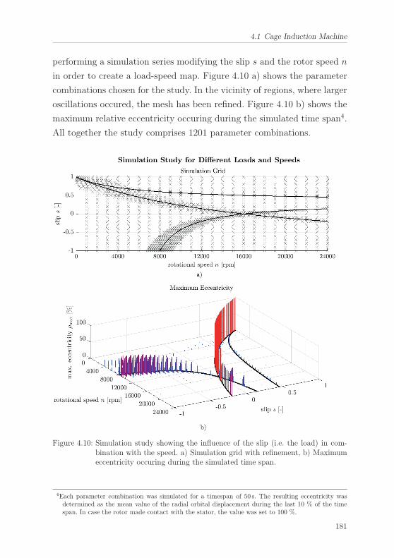
4.1 Cage Induction Machine
performing a simulation series modifying the slip s and the rotor speed n
in order to create a load-speed map. Figure 4.10 a) shows the parameter
combinations chosen for the study. In the vicinity of regions, where larger
oscillations occured, the mesh has been refined. Figure 4.10 b) shows the
maximum relative eccentricity occuring during the simulated time span4.
All together the study comprises 1201 parameter combinations.
Figure 4.10: Simulation study showing the influence of the slip (i.e. the load) in com-bination with the speed. a) Simulation grid with refinement, b) Maximumeccentricity occuring during the simulated time span.
4Each parameter combination was simulated for a timespan of 50 s. The resulting eccentricity wasdetermined as the mean value of the radial orbital displacement during the last 10 % of the timespan. In case the rotor made contact with the stator, the value was set to 100 %.
181
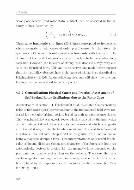
4 Results
Strong oscillations (and rotor-stator contact) can be observed in the vi-
cinity of lines described by(p
1− s− (p± 1)
)n ≈ ±ncrit. (4.1)
These zero harmonic slip lines (ZHS-lines) correspond to frequencies
where eccentricity field waves of order p ± 1 caused by the lateral ei-
genmotion of the rotor travel almost synchronously with the rotor. The
strength of the oscillation varies greatly from line to line and also along
each line. However, the location of strong oscillations is always very clo-
se to the identified lines. This and the observations made before suggest
that the instability observed here is the same which has been described by
Fruchtenicht et al. [20]. As the following discourse will show, the previous
findings can be generalised in certain points.
4.1.2 Generalisation: Physical Cause and Practical Assessment of
Self-Excited Rotor Oscillations due to the Rotor Cage
As mentioned in section 1.1, Fruchtenicht et al. calculated the eccentricity
fields of first order (p±1) corresponding to the fundamental field wave (or-
der p) for a circular orbital motion, based on a air-gap permeance theory.
They concluded that a magnetic force, which is caused by the interaction
of the fundamental and the eccentricity field waves and which is tangenti-
al to the orbit may excite the bending mode and thus lead to self-excited
vibrations. The authors interpreted this tangential force component as
being a magnetic damping force. This interpretation is only useful for cir-
cular orbits and disguises the natural character of the force: as it has been
axiomatically derived in section 2.1, the magnetic force depends on the
positional coordinates rather than on the velocity. Therefore, the term
electromagnetic damping force is intentionally avoided within this work,
but replaced by the expression electromagnetic cirulatory force (cf. Mer-
kin [96, p. 160]).
182
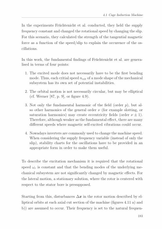
4.1 Cage Induction Machine
In the experiments Fruchtenicht et al. conducted, they held the supply
frequency constant and changed the rotational speed by changing the slip.
For this scenario, they calculated the strength of the tangential magnetic
force as a function of the speed/slip to explain the occurence of the os-
cillations.
In this work, the fundamental findings of Fruchtenicht et al. are genera-lised in terms of four points:
1. The excited mode does not necessarily have to be the first bendingmode. Thus, each critial speed ncrit of a mode shape of the mechanicalsubsystem has its own set of potential instabilities.
2. The orbital motion is not necessarily circular, but may be elliptical(cf. Werner [87, p. 9], or figure 4.9).
3. Not only the fundamental harmonic of the field (order p), but al-so other harmonics of the general order ν (for example slotting, orsaturation harmonics) may create eccentricity fields (order ν ± 1).Therefore, although weaker as the fundamental effect, there are manydifferent speeds where magnetic self-excited vibrations could occur.
4. Nowadays inverters are commonly used to change the machine speed.When considering the supply frequency variable (instead of only theslip), stability charts for the oscillations have to be provided in anappropriate form in order to make them useful.
To describe the excitation mechanism it is required that the rotational
speed ωr is constant and that the bending modes of the underlying me-
chanical subsystem are not significantly changed by magnetic effects. For
the lateral motion, a stationary solution, where the rotor is centered with
respect to the stator bore is presupposed.
Starting from this, disturbances Δx in the rotor motion described by el-
liptical orbits at each axial cut section of the machine (figures 4.11 a) and
b)) are assumed to occur. Their frequency is set to the natural frequen-
183
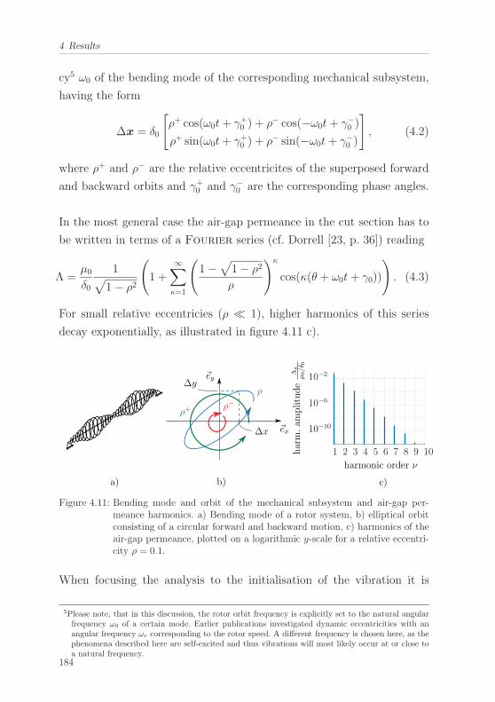
4 Results
cy5 ω0 of the bending mode of the corresponding mechanical subsystem,
having the form
Δx = δ0
[ρ+ cos(ω0t+ γ+0 ) + ρ− cos(−ω0t+ γ−0 )ρ+ sin(ω0t+ γ+0 ) + ρ− sin(−ω0t+ γ−0 )
], (4.2)
where ρ+ and ρ− are the relative eccentricites of the superposed forward
and backward orbits and γ+0 and γ−0 are the corresponding phase angles.
In the most general case the air-gap permeance in the cut section has to
be written in terms of a Fourier series (cf. Dorrell [23, p. 36]) reading
Λ =μ0δ0
1√1− ρ2
(1 +
∞∑κ=1
(1−√1− ρ2
ρ
)κ
cos(κ(θ + ω0t+ γ0))
). (4.3)
For small relative eccentricies (ρ � 1), higher harmonics of this series
decay exponentially, as illustrated in figure 4.11 c).
a) b) c)
�ey
ρ+
ρ
ρ−
Δx
Δy
1 2 3 4 5 6 7 8 9 10
�ex
harmonic order ν
harm.am
plitude
Λκ
μ0/δ 0
10−2
10−6
10−10
Figure 4.11: Bending mode and orbit of the mechanical subsystem and air-gap per-meance harmonics. a) Bending mode of a rotor system, b) elliptical orbitconsisting of a circular forward and backward motion, c) harmonics of theair-gap permeance, plotted on a logarithmic y-scale for a relative eccentri-city ρ = 0.1.
When focusing the analysis to the initialisation of the vibration it is
5Please note, that in this discussion, the rotor orbit frequency is explicitly set to the natural angularfrequency ω0 of a certain mode. Earlier publications investigated dynamic eccentricities with anangular frequency ωr corresponding to the rotor speed. A different frequency is chosen here, as thephenomena described here are self-excited and thus vibrations will most likely occur at or close toa natural frequency.
184
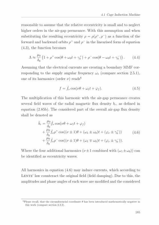
4.1 Cage Induction Machine
reasonable to assume that the relative eccentricity is small and to neglect
higher orders in the air-gap permeance. With this assumption and when
substituting the resulting eccentricity ρ = ρ(ρ+, ρ−) as a function of the
forward and backward orbits ρ+ and ρ− in the linearised form of equation
(4.3), the function becomes
Λ ≈ μ0δ0
(1 + ρ+ cos(θ + ω0t+ γ+0 ) + ρ− cos(θ − ω0t+ γ−0 )
). (4.4)
Assuming that the electrical currents are creating a boundary MMF cor-
responding to the supply angular frequency ω1 (compare section 2.5.1),
one of its harmonics (order ν) reads6
f = fν cos(νθ + ω1t+ ϕf). (4.5)
The multiplication of this harmonic with the air-gap permeance creates
several field waves of the radial magnetic flux density br, as defined in
equation (2.85b). The considered part of the overall air-gap flux density
shall be denoted as
br =μ0δ0fν cos(νθ + ω1t+ ϕf)
+μ0δ0fνρ
+ cos((ν ± 1)θ + (ω1 ± ω0)t+ (ϕν ± γ+0 ))
+μ0δ0fνρ
− cos((ν ± 1)θ + (ω1 ∓ ω0)t+ (ϕν ± γ−0 )).
(4.6)
Where the four additional harmonics (ν±1 combined with (ω1±ω0)) can
be identified as eccentricity waves.
All harmonics in equation (4.6) may induce currents, which according to
Lentz’ law counteract the original field (field damping). Due to this, the
amplitudes and phase angles of each wave are modified and the considered
6Please recall, that the circumferencial coordinate θ has been introduced mathematically negative inthis work (compare section 2.3.2).
185
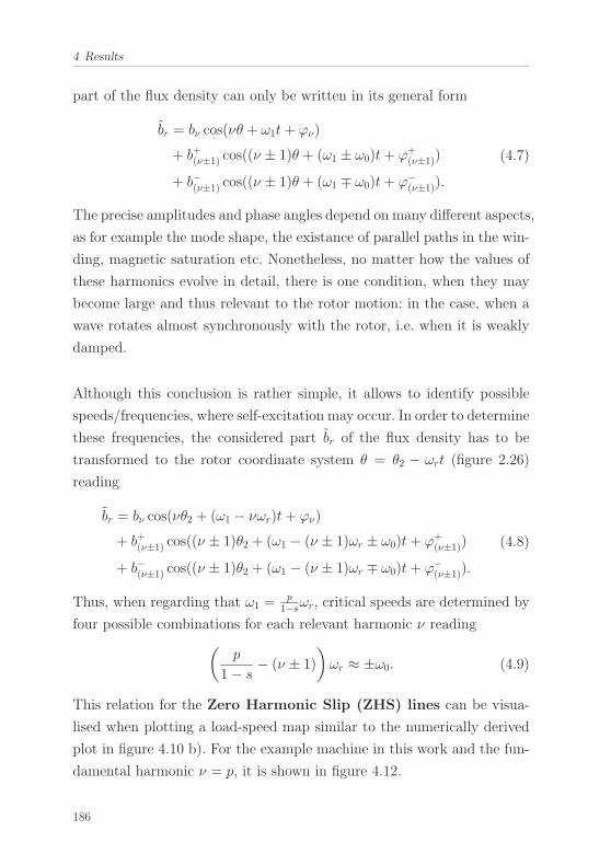
4 Results
part of the flux density can only be written in its general form
br = bν cos(νθ + ω1t+ ϕν)
+ b+(ν±1) cos((ν ± 1)θ + (ω1 ± ω0)t+ ϕ+(ν±1))
+ b−(ν±1) cos((ν ± 1)θ + (ω1 ∓ ω0)t+ ϕ−(ν±1)).
(4.7)
The precise amplitudes and phase angles depend on many different aspects,
as for example the mode shape, the existance of parallel paths in the win-
ding, magnetic saturation etc. Nonetheless, no matter how the values of
these harmonics evolve in detail, there is one condition, when they may
become large and thus relevant to the rotor motion: in the case, when a
wave rotates almost synchronously with the rotor, i.e. when it is weakly
damped.
Although this conclusion is rather simple, it allows to identify possible
speeds/frequencies, where self-excitation may occur. In order to determine
these frequencies, the considered part br of the flux density has to be
transformed to the rotor coordinate system θ = θ2 − ωrt (figure 2.26)
reading
br = bν cos(νθ2 + (ω1 − νωr)t+ ϕν)
+ b+(ν±1) cos((ν ± 1)θ2 + (ω1 − (ν ± 1)ωr ± ω0)t+ ϕ+(ν±1))
+ b−(ν±1) cos((ν ± 1)θ2 + (ω1 − (ν ± 1)ωr ∓ ω0)t+ ϕ−(ν±1)).
(4.8)
Thus, when regarding that ω1 =p
1−sωr, critical speeds are determined by
four possible combinations for each relevant harmonic ν reading(p
1− s− (ν ± 1)
)ωr ≈ ±ω0. (4.9)
This relation for the Zero Harmonic Slip (ZHS) lines can be visua-
lised when plotting a load-speed map similar to the numerically derived
plot in figure 4.10 b). For the example machine in this work and the fun-
damental harmonic ν = p, it is shown in figure 4.12.
186
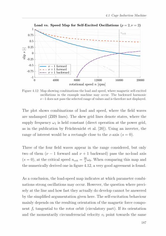
4.1 Cage Induction Machine
Figure 4.12: Map showing combinations the load and speed, where magnetic self-excitedoscillations in the example machine may occur. The backward harmonicν−1 does not pass the selected range of values and is therefore not displayed.
The plot shows combinations of load and speed, where the field waves
are undamped (ZHS lines). The skew grid lines denote states, where the
supply frequency ω1 is held constant (direct operation at the power grid,
as in the publication by Fruchtenicht et al. [20]). Using an inverter, the
range of interest would be a rectangle close to the x-axis (s = 0).
Three of the four field waves appear in the range considered, but only
two of them (ν − 1 forward and ν + 1 backward) pass the no-load axis
(s = 0), at the critical speed ncrit =30π ω0. When comparing this map and
the numerically derived one in figure 4.12, a very good agreement is found.
As a conclusion, the load-speed map indicates at which parameter combi-
nations strong oscillations may occur. However, the question where preci-
sely at the line and how fast they actually do develop cannot be answered
by the simplified argumentation given here. The self-excitation behaviour
mainly depends on the resulting orientation of the magnetic force compo-
nent ft tangential to the rotor orbit (circulatory part). If its orientation
and the momentarily circumferencial velocity vt point towards the same
187
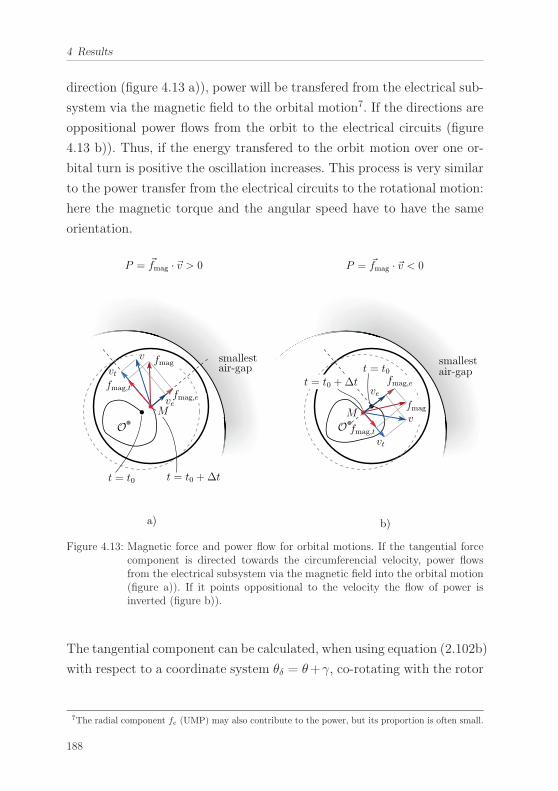
4 Results
direction (figure 4.13 a)), power will be transfered from the electrical sub-
system via the magnetic field to the orbital motion7. If the directions are
oppositional power flows from the orbit to the electrical circuits (figure
4.13 b)). Thus, if the energy transfered to the orbit motion over one or-
bital turn is positive the oscillation increases. This process is very similar
to the power transfer from the electrical circuits to the rotational motion:
here the magnetic torque and the angular speed have to have the same
orientation.
t = t0 +Δt
fmag
fmag,e
fmag,t
v
ve
vt
P = �fmag · �v < 0
a) b)
smallest
t = t0 t = t0 +Δt
fmag
fmag,e
fmag,t
v
ve
vt
P = �fmag · �v > 0
air-gapsmallestair-gap
M
O OM
t = t0
Figure 4.13: Magnetic force and power flow for orbital motions. If the tangential forcecomponent is directed towards the circumferencial velocity, power flowsfrom the electrical subsystem via the magnetic field into the orbital motion(figure a)). If it points oppositional to the velocity the flow of power isinverted (figure b)).
The tangential component can be calculated, when using equation (2.102b)
with respect to a coordinate system θδ = θ+γ, co-rotating with the rotor
7The radial component fe (UMP) may also contribute to the power, but its proportion is often small.
188
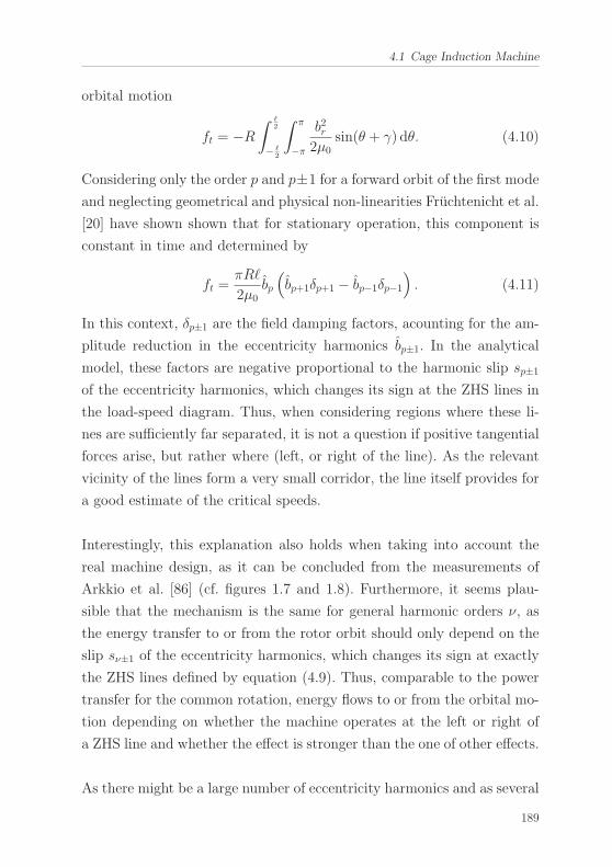
4.1 Cage Induction Machine
orbital motion
ft = −R∫ �
2
− �2
∫ π
−π
b2r2μ0
sin(θ + γ) dθ. (4.10)
Considering only the order p and p±1 for a forward orbit of the first mode
and neglecting geometrical and physical non-linearities Fruchtenicht et al.
[20] have shown shown that for stationary operation, this component is
constant in time and determined by
ft =πR�
2μ0bp
(bp+1δp+1 − bp−1δp−1
). (4.11)
In this context, δp±1 are the field damping factors, acounting for the am-
plitude reduction in the eccentricity harmonics bp±1. In the analytical
model, these factors are negative proportional to the harmonic slip sp±1
of the eccentricity harmonics, which changes its sign at the ZHS lines in
the load-speed diagram. Thus, when considering regions where these li-
nes are sufficiently far separated, it is not a question if positive tangential
forces arise, but rather where (left, or right of the line). As the relevant
vicinity of the lines form a very small corridor, the line itself provides for
a good estimate of the critical speeds.
Interestingly, this explanation also holds when taking into account the
real machine design, as it can be concluded from the measurements of
Arkkio et al. [86] (cf. figures 1.7 and 1.8). Furthermore, it seems plau-
sible that the mechanism is the same for general harmonic orders ν, as
the energy transfer to or from the rotor orbit should only depend on the
slip sν±1 of the eccentricity harmonics, which changes its sign at exactly
the ZHS lines defined by equation (4.9). Thus, comparable to the power
transfer for the common rotation, energy flows to or from the orbital mo-
tion depending on whether the machine operates at the left or right of
a ZHS line and whether the effect is stronger than the one of other effects.
As there might be a large number of eccentricity harmonics and as several
189
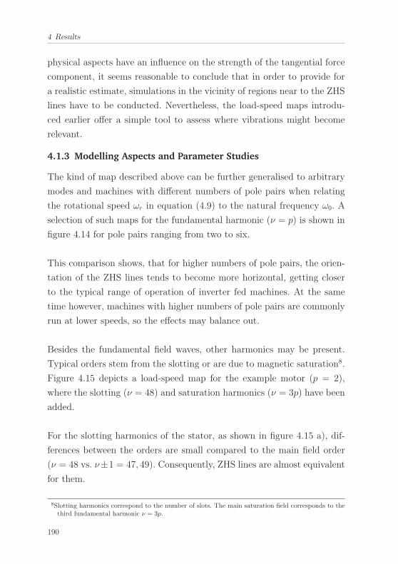
4 Results
physical aspects have an influence on the strength of the tangential force
component, it seems reasonable to conclude that in order to provide for
a realistic estimate, simulations in the vicinity of regions near to the ZHS
lines have to be conducted. Nevertheless, the load-speed maps introdu-
ced earlier offer a simple tool to assess where vibrations might become
relevant.
4.1.3 Modelling Aspects and Parameter Studies
The kind of map described above can be further generalised to arbitrary
modes and machines with different numbers of pole pairs when relating
the rotational speed ωr in equation (4.9) to the natural frequency ω0. A
selection of such maps for the fundamental harmonic (ν = p) is shown in
figure 4.14 for pole pairs ranging from two to six.
This comparison shows, that for higher numbers of pole pairs, the orien-
tation of the ZHS lines tends to become more horizontal, getting closer
to the typical range of operation of inverter fed machines. At the same
time however, machines with higher numbers of pole pairs are commonly
run at lower speeds, so the effects may balance out.
Besides the fundamental field waves, other harmonics may be present.
Typical orders stem from the slotting or are due to magnetic saturation8.
Figure 4.15 depicts a load-speed map for the example motor (p = 2),
where the slotting (ν = 48) and saturation harmonics (ν = 3p) have been
added.
For the slotting harmonics of the stator, as shown in figure 4.15 a), dif-
ferences between the orders are small compared to the main field order
(ν = 48 vs. ν±1 = 47, 49). Consequently, ZHS lines are almost equivalent
for them.
8Slotting harmonics correspond to the number of slots. The main saturation field corresponds to thethird fundamental harmonic ν = 3p.
190
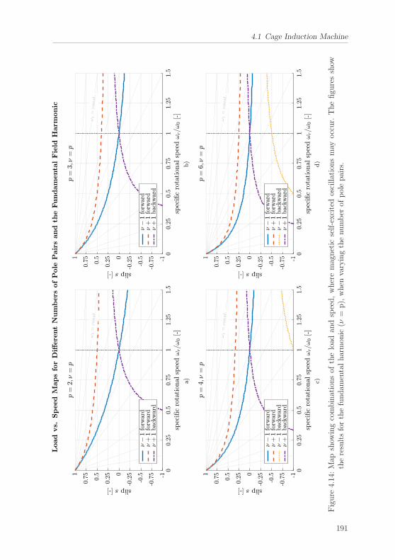
4.1 Cage Induction Machine
Figure
4.14:Map
show
ingcombinationsof
theload
andspeed,wheremagnetic
self-excitedoscillationsmay
occur.
Thefigu
resshow
theresultsforthefundam
entalharmon
ic(ν
=p),when
varyingthenumber
ofpolepairs.
191
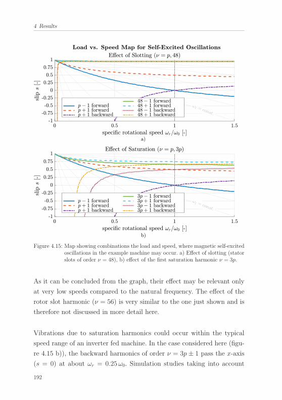
4 Results
Figure 4.15: Map showing combinations the load and speed, where magnetic self-excitedoscillations in the example machine may occur. a) Effect of slotting (statorslots of order ν = 48), b) effect of the first saturation harmonic ν = 3p.
As it can be concluded from the graph, their effect may be relevant only
at very low speeds compared to the natural frequency. The effect of the
rotor slot harmonic (ν = 56) is very similar to the one just shown and is
therefore not discussed in more detail here.
Vibrations due to saturation harmonics could occur within the typical
speed range of an inverter fed machine. In the case considered here (figu-
re 4.15 b)), the backward harmonics of order ν = 3p± 1 pass the x-axis
(s = 0) at about ωr = 0.25ω0. Simulation studies taking into account
192
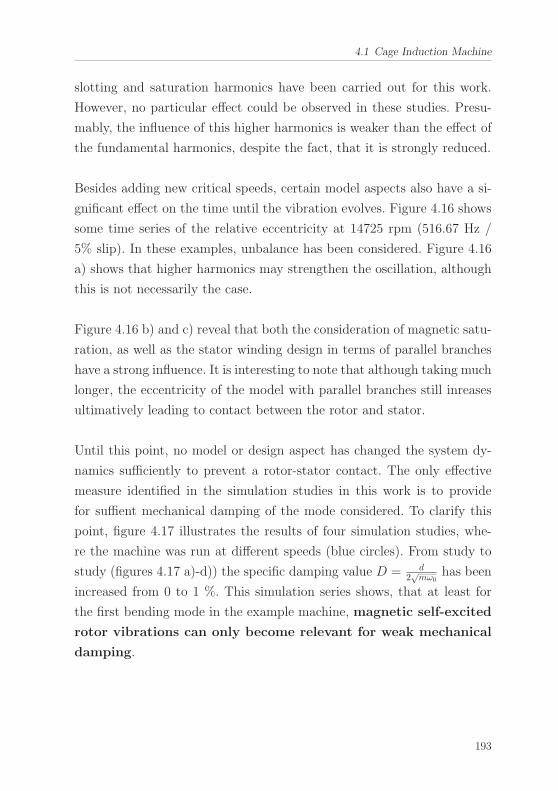
4.1 Cage Induction Machine
slotting and saturation harmonics have been carried out for this work.
However, no particular effect could be observed in these studies. Presu-
mably, the influence of this higher harmonics is weaker than the effect of
the fundamental harmonics, despite the fact, that it is strongly reduced.
Besides adding new critical speeds, certain model aspects also have a si-
gnificant effect on the time until the vibration evolves. Figure 4.16 shows
some time series of the relative eccentricity at 14725 rpm (516.67 Hz /
5% slip). In these examples, unbalance has been considered. Figure 4.16
a) shows that higher harmonics may strengthen the oscillation, although
this is not necessarily the case.
Figure 4.16 b) and c) reveal that both the consideration of magnetic satu-
ration, as well as the stator winding design in terms of parallel branches
have a strong influence. It is interesting to note that although taking much
longer, the eccentricity of the model with parallel branches still inreases
ultimatively leading to contact between the rotor and stator.
Until this point, no model or design aspect has changed the system dy-
namics sufficiently to prevent a rotor-stator contact. The only effective
measure identified in the simulation studies in this work is to provide
for suffient mechanical damping of the mode considered. To clarify this
point, figure 4.17 illustrates the results of four simulation studies, whe-
re the machine was run at different speeds (blue circles). From study to
study (figures 4.17 a)-d)) the specific damping value D = d2√mω0
has been
increased from 0 to 1 %. This simulation series shows, that at least for
the first bending mode in the example machine, magnetic self-excited
rotor vibrations can only become relevant for weak mechanical
damping.
193
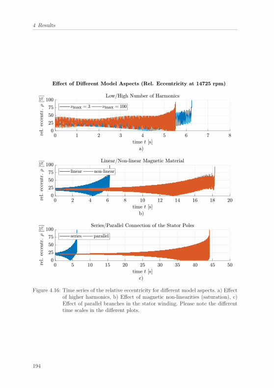
4 Results
Figure 4.16: Time series of the relative eccentricity for different model aspects. a) Effectof higher harmonics, b) Effect of magnetic non-linearities (saturation), c)Effect of parallel branches in the stator winding. Please note the differenttime scales in the different plots.
194
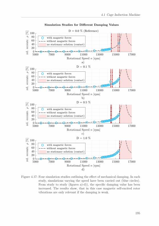
4.1 Cage Induction Machine
Figure 4.17: Four simulation studies outlining the effect of mechanical damping. In eachstudy, simulations varying the speed have been carried out (blue circles).From study to study (figures a)-d)), the specific damping value has beenincreased. The results show, that in this case magnetic self-excited rotorvibrations are only relevant if the damping is weak.
195
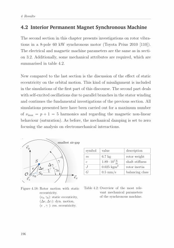
4 Results
4.2 Interior Permanent Magnet Synchronous Machine
The second section in this chapter presents investigations on rotor vibra-
tions in a 8-pole 60 kW synchronous motor (Toyota Prius 2010 [110]).
The electrical and magnetic machine parameters are the same as in secti-
on 3.2. Additionally, some mechanical attributes are required, which are
summarised in table 4.2.
New compared to the last section is the discussion of the effect of static
eccentricity on the orbital motion. This kind of misalignment is included
in the simulations of the first part of this discourse. The second part deals
with self-excited oscillations due to parallel branches in the stator winding
and continues the fundamental investigations of the previous section. All
simulations presented here have been carried out for a maximum number
of νmax = p + 1 = 5 harmonics and regarding the magnetic non-linear
behaviour (saturation). As before, the mechanical damping is set to zero
focusing the analysis on electromechanical interactions.
smallest air-gap
�ex
�ey
�ez
S
Oe
e0
γ
γ0ΔeΔγ
S0
Figure 4.18: Rotor motion with staticeccentricity.(e0, γ0): static eccenticity,(Δe,Δγ): dyn. motion,(e , γ ): res. eccentricity.
symbol value description
m 6.7 kg rotor weight
c 1.89 · 107 Nm
shaft stiffness
J 0.025 kgm2 rotor inertia
G 0.5 mm/s balancing class
Table 4.2: Overview of the most rele-vant mechanical parametersof the synchronous machine.
196
4.2 Interior Permanent Magnet Synchronous Machine
4.2.1 Simulation Studies
The Effect of Static Eccentricity on the Rotordynamic Motion
Static eccentricity is characterised by a constant offset (e0, γ0) of the rotor
shaft centre S from the stator bore centre O (figure 4.18). Typical causes
for static eccentricity are manufacturing errors, tolerances, or wear. If the
machine is operated, lateral forces act on the rotor creating an additional
time dependend rotordynamic motion (Δe(t),Δγ(t)). In the end, both
displacements result in a resulting eccentricity (e(t), γ(t)).
From a physical point of view it is to be expected, that the additional
static misalignment will affect the rotor orbital motion. This is due to the
circumstance, that the magnetic forces depend on the resulting eccentri-
city (the absolute air-gap width), while for most mechanical forces (shaft
restoring force, unbalance, etc.) only the dynamic motion is of relevance.
In the following, the qualitative solution behaviour under static eccen-
tricity is discussed. After that, some parameter studies in terms of the
absolute value of the static displacement, the load and the machine speed
will be presented. As before, the relative eccentricity ρ = eδm
is used to
assess the vibration behaviour.
In a first scenario simulations at 0% and 10% static eccentricity are com-
pared. In both cases, the machine is operated at constant speed (800Hz
/ 12000 rpm) and 40Nm load torque.
197
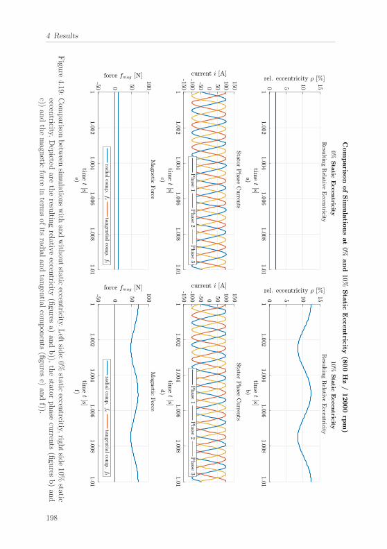
4 Results
Figu
re4.19:
Com
parison
betw
eensim
ulation
swith
andwith
outstatic
eccentricity.
Left
side:0%
staticeccen
trcitiy,righ
tsid
e10%
staticeccen
tricity.Depicted
aretheresu
ltingrelative
eccentricity
(figu
resa)
andb)),
thestator
phase
curren
ts(figu
resb)an
dc))
andthemagn
eticforce
interm
sof
itsrad
ialan
dtan
gential
compon
ents
(figu
rese)
andf)).
198
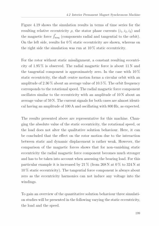
4.2 Interior Permanent Magnet Synchronous Machine
Figure 4.19 shows the simulation results in terms of time series for the
resulting relative eccentricity ρ, the stator phase currents (i1, i2, i3) and
the magnetic force �fmag (components radial and tangential to the orbit).
On the left side, results for 0% static eccentricity are shown, whereas on
the right side the simulation was run at 10% static eccentricity.
For the rotor without static misalignment, a constant resulting eccentri-
city of 1.95% is observed. The radial magnetic force is about 11N and
the tangential component is approximately zero. In the case with 10%
static eccentricity, the shaft centre motion forms a circular orbit with an
amplitude of 2.36% about an average value of 10.5%. The orbit frequency
corresponds to the rotational speed. The radial magnetic force component
oscillates similar to the eccentricity with an amplitude of 10N about an
average value of 59N. The current signals for both cases are almost identi-
cal having an amplitude of 100A and oscillating with 800Hz, as expected.
The results presented above are representative for this machine. Chan-
ging the absolute value of the static eccentricity, the rotational speed, or
the load does not alter the qualitative solution behaviour. Here, it can
be concluded that the effect on the rotor motion due to the interaction
between static and dynamic displacement is rather weak. However, the
comparison of the magnetic forces shows that for non-vanishing static
eccentricity the radial magnetic force component becomes much stronger
and has to be taken into account when assessing the bearing load. For this
particular example it is increased by 21% (from 268N at 0% to 324N at
10% static eccentricity). The tangential force component is always about
zero as the eccentricity harmonics can not induce any voltage into the
windings.
To gain an overview of the quantitative solution behaviour three simulati-
on studies will be presented in the following varying the static eccentricity,
the load and the speed.
199
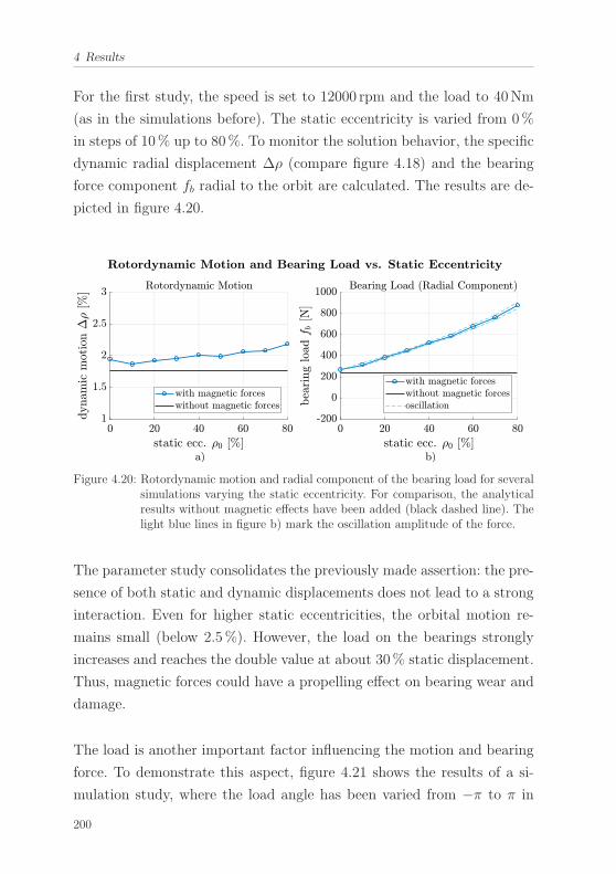
4 Results
For the first study, the speed is set to 12000 rpm and the load to 40Nm
(as in the simulations before). The static eccentricity is varied from 0%
in steps of 10% up to 80%. To monitor the solution behavior, the specific
dynamic radial displacement Δρ (compare figure 4.18) and the bearing
force component fb radial to the orbit are calculated. The results are de-
picted in figure 4.20.
Figure 4.20: Rotordynamic motion and radial component of the bearing load for severalsimulations varying the static eccentricity. For comparison, the analyticalresults without magnetic effects have been added (black dashed line). Thelight blue lines in figure b) mark the oscillation amplitude of the force.
The parameter study consolidates the previously made assertion: the pre-
sence of both static and dynamic displacements does not lead to a strong
interaction. Even for higher static eccentricities, the orbital motion re-
mains small (below 2.5%). However, the load on the bearings strongly
increases and reaches the double value at about 30% static displacement.
Thus, magnetic forces could have a propelling effect on bearing wear and
damage.
The load is another important factor influencing the motion and bearing
force. To demonstrate this aspect, figure 4.21 shows the results of a si-
mulation study, where the load angle has been varied from −π to π in
200
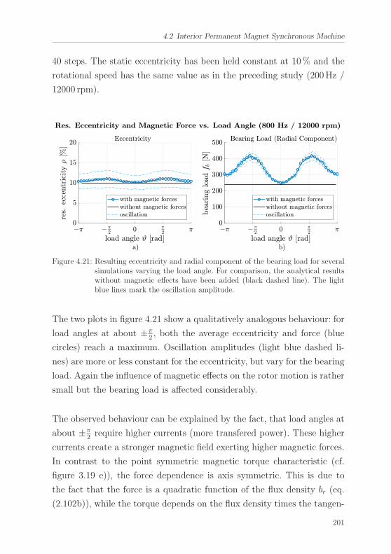
4.2 Interior Permanent Magnet Synchronous Machine
40 steps. The static eccentricity has been held constant at 10% and the
rotational speed has the same value as in the preceding study (200Hz /
12000 rpm).
Figure 4.21: Resulting eccentricity and radial component of the bearing load for severalsimulations varying the load angle. For comparison, the analytical resultswithout magnetic effects have been added (black dashed line). The lightblue lines mark the oscillation amplitude.
The two plots in figure 4.21 show a qualitatively analogous behaviour: for
load angles at about ±π2 , both the average eccentricity and force (blue
circles) reach a maximum. Oscillation amplitudes (light blue dashed li-
nes) are more or less constant for the eccentricity, but vary for the bearing
load. Again the influence of magnetic effects on the rotor motion is rather
small but the bearing load is affected considerably.
The observed behaviour can be explained by the fact, that load angles at
about ±π2 require higher currents (more transfered power). These higher
currents create a stronger magnetic field exerting higher magnetic forces.
In contrast to the point symmetric magnetic torque characteristic (cf.
figure 3.19 e)), the force dependence is axis symmetric. This is due to
the fact that the force is a quadratic function of the flux density br (eq.
(2.102b)), while the torque depends on the flux density times the tangen-
201
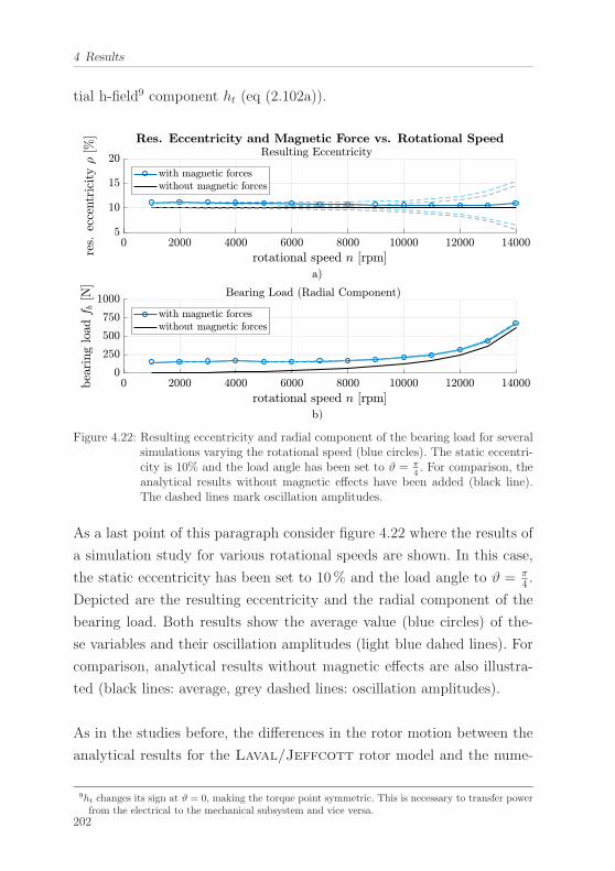
4 Results
tial h-field9 component ht (eq (2.102a)).
Figure 4.22: Resulting eccentricity and radial component of the bearing load for severalsimulations varying the rotational speed (blue circles). The static eccentri-city is 10% and the load angle has been set to ϑ = π
4. For comparison, the
analytical results without magnetic effects have been added (black line).The dashed lines mark oscillation amplitudes.
As a last point of this paragraph consider figure 4.22 where the results of
a simulation study for various rotational speeds are shown. In this case,
the static eccentricity has been set to 10% and the load angle to ϑ = π4 .
Depicted are the resulting eccentricity and the radial component of the
bearing load. Both results show the average value (blue circles) of the-
se variables and their oscillation amplitudes (light blue dahed lines). For
comparison, analytical results without magnetic effects are also illustra-
ted (black lines: average, grey dashed lines: oscillation amplitudes).
As in the studies before, the differences in the rotor motion between the
analytical results for the Laval/Jeffcott rotor model and the nume-
9ht changes its sign at ϑ = 0, making the torque point symmetric. This is necessary to transfer powerfrom the electrical to the mechanical subsystem and vice versa.
202
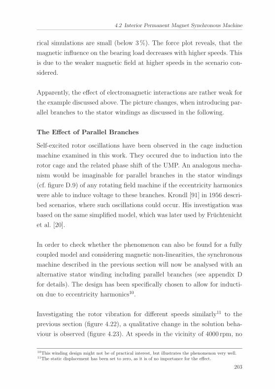
4.2 Interior Permanent Magnet Synchronous Machine
rical simulations are small (below 3%). The force plot reveals, that the
magnetic influence on the bearing load decreases with higher speeds. This
is due to the weaker magnetic field at higher speeds in the scenario con-
sidered.
Apparently, the effect of electromagnetic interactions are rather weak for
the example discussed above. The picture changes, when introducing par-
allel branches to the stator windings as discussed in the following.
The Effect of Parallel Branches
Self-excited rotor oscillations have been observed in the cage induction
machine examined in this work. They occured due to induction into the
rotor cage and the related phase shift of the UMP. An analogous mecha-
nism would be imaginable for parallel branches in the stator windings
(cf. figure D.9) of any rotating field machine if the eccentricity harmonics
were able to induce voltage to these branches. Krondl [91] in 1956 descri-
bed scenarios, where such oscillations could occur. His investigation was
based on the same simplified model, which was later used by Fruchtenicht
et al. [20].
In order to check whether the phenomenon can also be found for a fully
coupled model and considering magnetic non-linearities, the synchronous
machine described in the previous section will now be analysed with an
alternative stator winding including parallel branches (see appendix D
for details). The design has been specifically chosen to allow for inducti-
on due to eccentricity harmonics10.
Investigating the rotor vibration for different speeds similarly11 to the
previous section (figure 4.22), a qualitative change in the solution beha-
viour is observed (figure 4.23). At speeds in the vicinity of 4000 rpm, no
10This winding design might not be of practical interest, but illustrates the phenomenon very well.11The static displacement has been set to zero, as it is of no importance for the effect.
203
4 Results
Figure 4.23: Resulting eccentricity for a winding design with parallel branches varyingthe rotational speed (blue circles). The load angle has been set to ϑ = π
4.
For comparison, the analytical results without magnetic effects have beenadded (black line). The red area marks speeds where no stationary solutioncould be found and the rotor made contact with the stator.
stationary solution can be found: instead, the vibration increases until
the rotor makes contact with the stator.
Figure 4.24 shows time series of this process at 4000 rpm. For comparison,
the results at 3800 rpm are also depicted.
When considering the relative x-displacement for a short time intervall
(figure 4.24 a)), it turns out that at 4000 rpm the original oscillation due
to unbalance is modulated by another increasing vibration component of
about four times the rotation frequency. Taking a look at the long term be-
haviour of the relative eccentricity (4.24 b)) reveals that the displacement
increases steadily until the rotor makes contact with the stator. Regar-
ding the orbits in figures 4.24 c)-e) shows, that the secondary oscillation
changes the orbital shape from initially circular to elliptical. Furthermore,
the orbital direction is changed from forward to backward.
From the spectrogram in figure 4.25 a) a frequency of about 261Hz for
the secondary oscillation can be deduced. The frequency of the unbalan-
204
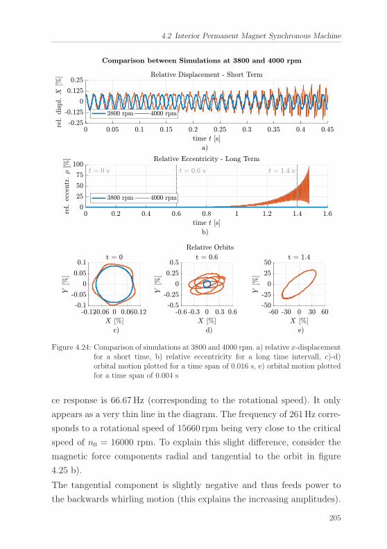
4.2 Interior Permanent Magnet Synchronous Machine
Figure 4.24: Comparison of simulations at 3800 and 4000 rpm. a) relative x-displacementfor a short time, b) relative eccentricity for a long time intervall, c)-d)orbital motion plotted for a time span of 0.016 s, e) orbital motion plottedfor a time span of 0.004 s
ce response is 66.67Hz (corresponding to the rotational speed). It only
appears as a very thin line in the diagram. The frequency of 261Hz corre-
sponds to a rotational speed of 15660 rpm being very close to the critical
speed of n0 = 16000 rpm. To explain this slight difference, consider the
magnetic force components radial and tangential to the orbit in figure
4.25 b).
The tangential component is slightly negative and thus feeds power to
the backwards whirling motion (this explains the increasing amplitudes).
205
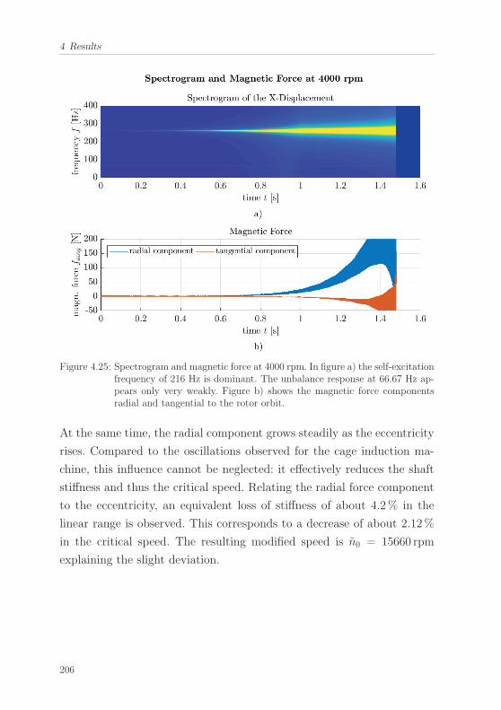
4 Results
Figure 4.25: Spectrogram and magnetic force at 4000 rpm. In figure a) the self-excitationfrequency of 216 Hz is dominant. The unbalance response at 66.67 Hz ap-pears only very weakly. Figure b) shows the magnetic force componentsradial and tangential to the rotor orbit.
At the same time, the radial component grows steadily as the eccentricity
rises. Compared to the oscillations observed for the cage induction ma-
chine, this influence cannot be neglected: it effectively reduces the shaft
stiffness and thus the critical speed. Relating the radial force component
to the eccentricity, an equivalent loss of stiffness of about 4.2% in the
linear range is observed. This corresponds to a decrease of about 2.12%
in the critical speed. The resulting modified speed is n0 = 15660 rpm
explaining the slight deviation.
206
4.2 Interior Permanent Magnet Synchronous Machine
In conclusion, the simulation study for parallel branches in the stator
winding lead to a magnetic self-excited rotor oscillation at a rotor speed
of
n =n04. (4.12)
As for the former example, this relation can be generalised for arbitrary
situations involving parallel branches in a stator winding, as discussed
subsequently.
4.2.2 Generalisation: Physical Cause and Practical Assessment of
Self-Excited Rotor Oscillations due to Parallel Branches
The explanation for magnetic self-excited rotor oscillations due to parallel
branches in the stator winding follows a very similar argumentary as
for the cage induction machine (compare section 4.1.2). Calculating the
eccentricity harmonics of a certain magnetic flux density wave of order ν
for an elliptical orbit yields
br = bν cos(νθ + ω1t+ ϕν)
+ b+ν±1 cos((ν ± 1)θ + (ω1 ± ω0)t+ ϕ+(ν±1))
+ b−ν±1 cos((ν ± 1)θ + (ω1 ∓ ω0)t+ ϕ−(ν±1)),
(4.13)
where in this case ω0 is the reduced natural frequency of a certain mode
shape. In the case of the cage induction machine it turned out, that
eccentricity harmonics may cause strong oscillations when rotating almost
synchronously to the rotor. For parallel branches, these harmonics have
to almost stand still. Regarding ω1 = pωr leads to the general condition
ωr ≈ ω0
p. (4.14)
Please note, that self-excited oscillations in this form can only occur if
the eccentrcitiy harmonics can induce voltage to the parallel branches.
This has to be checked for each winding design individually.
207
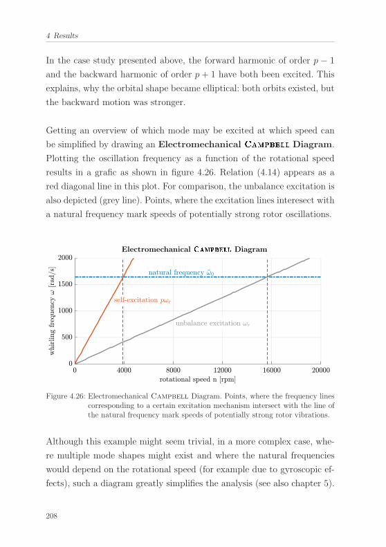
4 Results
In the case study presented above, the forward harmonic of order p − 1
and the backward harmonic of order p + 1 have both been excited. This
explains, why the orbital shape became elliptical: both orbits existed, but
the backward motion was stronger.
Getting an overview of which mode may be excited at which speed can
be simplified by drawing an Electromechanical Diagram.
Plotting the oscillation frequency as a function of the rotational speed
results in a grafic as shown in figure 4.26. Relation (4.14) appears as a
red diagonal line in this plot. For comparison, the unbalance excitation is
also depicted (grey line). Points, where the excitation lines interesect with
a natural frequency mark speeds of potentially strong rotor oscillations.
Electromechanical Diagram
Figure 4.26: Electromechanical Campbell Diagram. Points, where the frequency linescorresponding to a certain excitation mechanism intersect with the line ofthe natural frequency mark speeds of potentially strong rotor vibrations.
Although this example might seem trivial, in a more complex case, whe-
re multiple mode shapes might exist and where the natural frequencies
would depend on the rotational speed (for example due to gyroscopic ef-
fects), such a diagram greatly simplifies the analysis (see also chapter 5).
208
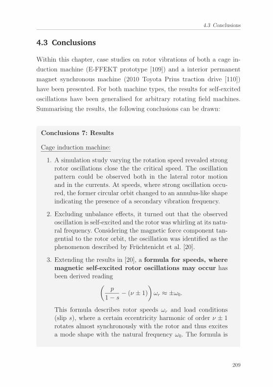
4.3 Conclusions
4.3 Conclusions
Within this chapter, case studies on rotor vibrations of both a cage in-
duction machine (E-FFEKT prototype [109]) and a interior permanent
magnet synchronous machine (2010 Toyota Prius traction drive [110])
have been presented. For both machine types, the results for self-excited
oscillations have been generalised for arbitrary rotating field machines.
Summarising the results, the following conclusions can be drawn:
Conclusions 7: Results
Cage induction machine:
1. A simulation study varying the rotation speed revealed strongrotor oscillations close the the critical speed. The oscillationpattern could be observed both in the lateral rotor motionand in the currents. At speeds, where strong oscillation occu-red, the former circular orbit changed to an annulus-like shapeindicating the presence of a secondary vibration frequency.
2. Excluding unbalance effects, it turned out that the observedoscillation is self-excited and the rotor was whirling at its natu-ral frequency. Considering the magnetic force component tan-gential to the rotor orbit, the oscillation was identified as thephenomenon described by Fruchtenicht et al. [20].
3. Extending the results in [20], a formula for speeds, wheremagnetic self-excited rotor oscillations may occur hasbeen derived reading(
p
1− s− (ν ± 1)
)ωr ≈ ±ω0.
This formula describes rotor speeds ωr and load conditions(slip s), where a certain eccentricity harmonic of order ν ± 1rotates almost synchronously with the rotor and thus excitesa mode shape with the natural frequency ω0. The formula is
209
4 Results
valid for all mode shapes describing cirular or elliptical orbits,for arbitrary harmonic orders ν and all kinds of cage inductionmachines with different numbers of pole pairs p.
4. Plotting the derived formula in a load-speed map (slip vs. rpm)lines of potential self-excitation (zero harmonic slip (ZHS)lines) can be identified. The occurence of these oscillations hasbeen numerically checked with very good agreement for thefundamental harmonic. Oscillations due to saturation harmo-nics or slotting have not been observed. The fact, that strongoscillations can only occur close to the ZHS lines is due tothe strong field damping if the eccentricity harmonics do notrotate nearly synchronous to the rotor.
5. For the practical assessment whether self-excited rotor oscilla-tions may appear, it is proposed to use numerical simulationclose to the ZHS lines. An analytical assessment seems not fea-sible, as magnetic forces are strongly influenced by saturation,load, the winding design and further aspects (cf. [86]).
6. From a simulation study varying the mechanical damping itwas concluded, that at least for the machine considered inthis work, self-excited oscillations are only relevant forweakly damped modes.
Interior permanent magnet synchronous machine
1. Investigating the effect of static eccentricity, several parameterstudies have been presented. These concerned variations ofthe value of the static displacement, the load and the speed.As a main result it turned out, that for a series connectionof the stator winding the electromechanical interaction canbe considered weak. However, it was also found, that staticeccentricity has a strong effect on the bearing load and thusmay significantly contribute to the bearing wear.
2. Introducing an alternative winding design, which involved par-allel branches in the stator winding, strong rotor oscillationshave been observed at about 4000 rpm corresponding to the
210
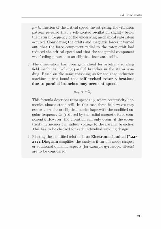
4.3 Conclusions
p− th fraction of the critical speed. Investigating the vibrationpattern revealed that a self-excited oscillation slightly belowthe natural frequency of the underlying mechanical subsystemoccured. Considering the orbits and magnetic forces it turnedout, that the force component radial to the rotor orbit hadreduced the critical speed and that the tangential componentwas feeding power into an elliptical backward orbit.
3. The observation has been generalised for arbitrary rotatingfield machines involving parallel branches in the stator win-ding. Based on the same reasoning as for the cage inductionmachine it was found that self-excited rotor vibrationsdue to parallel branches may occur at speeds
pωr ≈ ±ω0.
This formula describes rotor speeds ωr, where eccentricity har-monics almost stand still. In this case these field waves mayexcite a circular or elliptical mode shape with the modified an-gular frequency ω0 (reduced by the radial magnetic force com-ponent). However, the vibration can only occur, if the eccen-tricity harmonics can induce voltage to the parallel branches.This has to be checked for each individual winding design.
4. Plotting the identified relation in anElectromechanical ��������� Diagram simplifies the analysis if various mode shapes,or additional dynamic aspects (for example gyroscopic effects)are to be considered.
211
5 Conclusions and Suggestions forFurther Work
In the past decades, applications for rotating field electrical machines ha-
ve changed significantly. New technological fields, as for example electric
mobility, require a higher power density compared to earlier applications.
To achieve this aim, design concepts tend towards light weight structures
and higher rotational speeds. However, higher speeds and lighter struc-
tures tend to stronger vibration issues.
Based on this motivation an electromechanical model to describe magne-
tic excited lateral rotor oscillations has been developed within this work.
Compared to earlier approaches it accounts for the full coupling between
electric currents and the mechanical motion. The model covers both geo-
metrical non-linearities due to large and arbitrary orbital motions, as well
as saturation effects due to the physical non-linearity of the involved ma-
terials. It is applicable to all kinds of rotating field machines involving
any desired winding design and rotor topologies. Its numerical implemen-
tation has been designed to allow for long-term transient simulations and
large parameter studies. As the approach is two dimensional, only sym-
metrical bending modes can be considered. Three dimensional effects due
to skewing, or homopolar fluxes are not included. Furthermore, the skin
and proximity effects are not accounted for.
Deriving the governing equations, the modelling task has been subdivided
into three subproblems: the mechanical part, the electrical circuits
and themagnetic field problem. All equations have been derived based
212
on two different axiomatic approaches: the Newton-Faraday equations
(classical dynamics) and based on an energy principle: the Lagrange-
Maxwell equations (analytical dynamics).
Comparing both methods assured the energetical consistency for the ap-
proximations made within the derivation of the governing equations. Fur-
thermore, it has been proven, that lateral magnetic forces are either con-
servative, or of circulatory character (compare Merkin [96, p.160]). Ma-
gnetic damping forces are physically impossible, as the energy is only
transfered by the magnetic field. Dissipation can only take place in the
electrical, or the mechanical subsystems. This aspect may have significant
consequences for the assertion of lateral rotor oscillations.
Themechanical part has been modelled as a classical Laval/Jeffcott
rotor. This model allows for a very simple analyis and covers fundental
bending aspects. Furthermore, it can be extended straightforward towards
other mode shapes. The kinematics of this subproblem have been defined
to account for arbitrary orbital motion and including static eccentricities.
The electrical circuits have been described introducing so-called gene-
ralised meshes. Defining current variables, which can split between par-
allel branches, or circulate in between them, a minimum set of equations
has been derived. The equivalence between this approach and the common
nodal analysis has been proven. In the end, the description corresponds
to analytical dynamics of electrical networks and the introduced current
variables are generalised coordinates in the sense of Lagrangian dyna-
mics.
For the magnetic field problem the two dimensional domain has be-
en split into the air-gap and the surrounding solid regions. Within this
work, the air-gap has been defined as an annulus-shaped region between
stator and rotor without any slots or saliency. The latter have been ac-
213
5 Conclusions and Suggestions for Further Work
counted for in the solid parts. The solution for the air-gap domain has
been derived using an asymptotic expansion of the scalar magnetic po-
tential. Thus, an approximative solution has been derived directly from
Maxwell’s equations. The first order approximation of this solution is
consistent with the common air-gap permeance theories and allows for
a direct calculation of the magnetic energy based on the scalar potenti-
al. This approximation has been coupled to magnetic equivalent circuits
describing the solid parts (and slots/saliency) of the machine. The so mo-
dified semi-analytical AN-MEC method features very fast convergence
of the involved non-linear equation system and allows for fast time step-
ping simulations.
The model has been implemented in MATLAB, where the air-gap
field is expressed as a fourier-series using the FFT algorithm in each time
step. This allows to consider only certain harmonics of interest and signifi-
cantly increases the computational efficiency. The resulting system of dif-
ferential equations is solved using anAdams-Bashforth-Moulton sol-
ver. The non-linear magnetic field problem is solved using the Newton-
Raphson algorithm in every time step.
Based on the terminology of the SCS technical committee on model cre-
dibility [134], the implementation has been validated by comparing it
to finite element simulations, space vector models and experi-
mental data. To this end, two example machines have been considered:
a 50 kW 4-pole cage induction machine (E-FFEKT prototype [109]) and
a 60 kW 8-pole interior permanent magnet synchronous machine (2010
Toyota Prius traction drive [110]). Overall, a good agreement has been
found. The involved errors have been evaluated stochastically leading to
expected values below 3% and standard deviations below 11%. Larger
errors occured in the air-gap field of the synchronous machine, where an
iron bridge separates the magnet from the air-gap. As it turned out, the
discretisation using magnetic equivalent circuits can only approximate
214
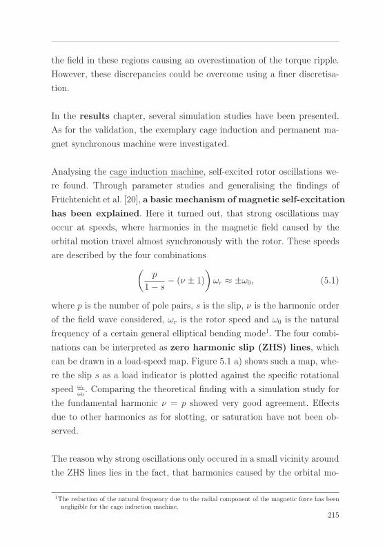
the field in these regions causing an overestimation of the torque ripple.
However, these discrepancies could be overcome using a finer discretisa-
tion.
In the results chapter, several simulation studies have been presented.
As for the validation, the exemplary cage induction and permanent ma-
gnet synchronous machine were investigated.
Analysing the cage induction machine, self-excited rotor oscillations we-
re found. Through parameter studies and generalising the findings of
Fruchtenicht et al. [20], a basic mechanism of magnetic self-excitation
has been explained. Here it turned out, that strong oscillations may
occur at speeds, where harmonics in the magnetic field caused by the
orbital motion travel almost synchronously with the rotor. These speeds
are described by the four combinations(p
1− s− (ν ± 1)
)ωr ≈ ±ω0, (5.1)
where p is the number of pole pairs, s is the slip, ν is the harmonic order
of the field wave considered, ωr is the rotor speed and ω0 is the natural
frequency of a certain general elliptical bending mode1. The four combi-
nations can be interpreted as zero harmonic slip (ZHS) lines, which
can be drawn in a load-speed map. Figure 5.1 a) shows such a map, whe-
re the slip s as a load indicator is plotted against the specific rotational
speed ωr
ω0. Comparing the theoretical finding with a simulation study for
the fundamental harmonic ν = p showed very good agreement. Effects
due to other harmonics as for slotting, or saturation have not been ob-
served.
The reason why strong oscillations only occured in a small vicinity around
the ZHS lines lies in the fact, that harmonics caused by the orbital mo-
1The reduction of the natural frequency due to the radial component of the magnetic force has beennegligible for the cage induction machine.
215

5 Conclusions and Suggestions for Further Work
tion are strongly reduced by counter induction when moving relative to
the rotor. As the actual vibration behaviour depends on many physical
aspects like saturation, higher harmonics, load, or the winding design, it
has been proposed to use numerical simulation in the vicinity of the ZHS
lines to provide for a realistic assessment of the occuring vibration.
Figure 5.1: Assessing magnetic self-excited rotor oscillations in rotating field electricalmachines. a) Load-speed map for a 4-pole cage induction machine (funda-mental harmonic), b) Electromechanical Campbell Diagram for a 8-polepermanent magnet synchronous machine with parallel branches in the sta-tor winding.
Considering the effect of mechanical dissipation it turned out, that at
least in the machine considered in this work, magnetic self-excited os-
cillations were only relevant for weak mechanical damping.
For the permanent magnet sychronous machine, two different aspects ha-
ve been analysed: first, the effect of static eccentricity on the dynamic
orbit has been investigated and second, self-excited oscillations due to
parallel branches in the stator winding have been discussed.
The effect of static eccentricity on the dynamic rotor motion tur-
ned out to be weak if the stator coils were connected in series. However, a
considerable increase in the bearing load has been observed, which should
216
be taken into account assessing the lifetime of the system.
In the second part concerning the synchronous machine an alternative
winding design has been investigated. This modified machine showed self-
excited rotor oscillations due to parallel branches in the vicinity
of
ωr ≈ ω0
p. (5.2)
The relation has been derived using a similar argumentation as for the ca-
ge induction machine. In this context ω0 is the reduced natural frequency
of a certain bending mode. The reduction in the natural frequency stems
from the radial component of the magnetic force. In contrast to the cage
induction machine, this reduction has not been negligible in this case.
Equation (5.2) is generally valid for self-excited vibrations due to parallel
branches in the stator windings, if the eccentricity harmonics caused by
the orbital motion can induce voltage to the parallel branches. This lat-
ter condition has to be checked for each winding individually. The critical
speed can be visualised in terms of an Electromechanical ��������
Diagram, as shown in figure 5.1 b). Although this example may appe-
ar rather trivial, the graphical interpretation may simplify the analysis
if several modes are considered and additional aspects (like gyroscopic
effects) play a role.
217
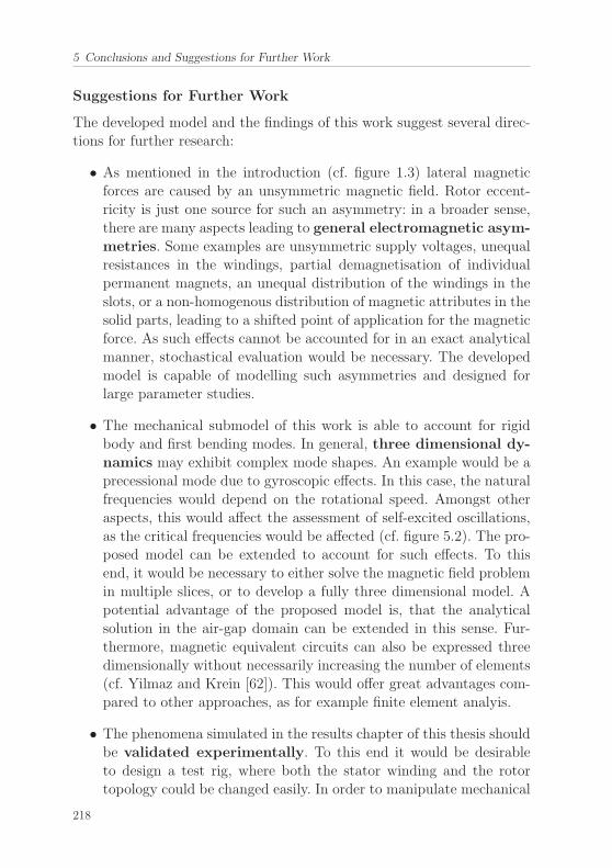
5 Conclusions and Suggestions for Further Work
Suggestions for Further Work
The developed model and the findings of this work suggest several direc-tions for further research:
• As mentioned in the introduction (cf. figure 1.3) lateral magneticforces are caused by an unsymmetric magnetic field. Rotor eccent-ricity is just one source for such an asymmetry: in a broader sense,there are many aspects leading to general electromagnetic asym-metries. Some examples are unsymmetric supply voltages, unequalresistances in the windings, partial demagnetisation of individualpermanent magnets, an unequal distribution of the windings in theslots, or a non-homogenous distribution of magnetic attributes in thesolid parts, leading to a shifted point of application for the magneticforce. As such effects cannot be accounted for in an exact analyticalmanner, stochastical evaluation would be necessary. The developedmodel is capable of modelling such asymmetries and designed forlarge parameter studies.
• The mechanical submodel of this work is able to account for rigidbody and first bending modes. In general, three dimensional dy-namics may exhibit complex mode shapes. An example would be aprecessional mode due to gyroscopic effects. In this case, the naturalfrequencies would depend on the rotational speed. Amongst otheraspects, this would affect the assessment of self-excited oscillations,as the critical frequencies would be affected (cf. figure 5.2). The pro-posed model can be extended to account for such effects. To thisend, it would be necessary to either solve the magnetic field problemin multiple slices, or to develop a fully three dimensional model. Apotential advantage of the proposed model is, that the analyticalsolution in the air-gap domain can be extended in this sense. Fur-thermore, magnetic equivalent circuits can also be expressed threedimensionally without necessarily increasing the number of elements(cf. Yilmaz and Krein [62]). This would offer great advantages com-pared to other approaches, as for example finite element analyis.
• The phenomena simulated in the results chapter of this thesis shouldbe validated experimentally. To this end it would be desirableto design a test rig, where both the stator winding and the rotortopology could be changed easily. In order to manipulate mechanical
218
parameters, magnetic bearings could be used (cf. [86]). Furthermore,it would be interesting to directly observe the rotor orbital motioninstead of just monitoring the bearing motion.
• The proposed model has been implemented in MATLAB. Althoughthe computational efficiency has reached a satisfactory level al-ready, there still is much potential to improve the computation time.To achieve this it would make sense to design an individual solver ac-counting for the peculiarities of the method (or to further investigatewhich combination of existent solvers is the fastest). Furthermore,calculating stationary solutions could be done by direct numericalapproximation methods, as for example the Harmonic Balance Me-thod (cf. Nayfeh and Balachandran [137]).
• Some simulations indicated the existence of nonlinear dynamic phe-nomena (see also Holopainen and Arkkio [94] for an experimental ex-ample). To investigate this, methods from nonlinear dynamics couldbe applied to the model, or a simplified minimal model could bededuced from the proposed one.
Figure 5.2: Self-excited rotor vibrations considering gyroscopic effects. a) Load-speedmap with additional ZHS lines due to the splitting of natural frequencies,b) Electromechanical Campbell Diagramm with additional speeds of self-excitation due to the splitting of natural frequencies. Note that these mapsare theoretical predictions and have not been validated.
219
References
[1] S. Chapman. Electric machinery fundamentals. Tata McGraw-Hill
Education, New York, USA, 2005.
[2] K. Rajashekara. Present status and future trends in electric vehicle
propulsion technologies. IEEE Journal of Emerging and Selected
Topics in Power Electronics, 1(1):3–10, 2013.
[3] S. Li, Y. Li, W. Choi, and B. Sarlioglu. High-speed electric machi-
nes: Challenges and design considerations. IEEE Transactions on
Transportation Electrification, 2(1):2–13, 2016.
[4] T. Burress. Electrical Performance, Reliability Analysis, and Cha-
racterization (of current Electric Vehicle Technologies). Oak Ridge
National Laboratory, U.S. Department of Energy Vehicle Technolo-
gies, Oak Ridge, USA, 2017.
[5] 5 seasons, 5 versions: Everything you need to know about our race
car, 2018. URL https://www.mahindraracing.com/blog/5-seasons-
5-versions-everything-you-need-to-know-about-our-race-car. Re-
trieved on 7/22/2019.
[6] Web of science [v.5.32], 2019. URL apps.webofknowledge.com. Re-
trieved on 6/25/2019.
[7] R. Gasch, R. Nordmann, and H. Pfutzner. Rotordynamik [(in Ger-
man) Rotordynamics]. Springer-Verlag, Berlin, Germany, 2006.
[8] W. Kellenberger. Der magnetische Zug in Turbogenerator-Rotoren
als Ursache einer Instabilitat des mechanischen Laufes [(in German)
220
References
The unbalanced magnetic pull in turbogenerator rotors as a source
for instability of the mechanical motion]. Archiv fur Elektrotechnik,
50(4):253–265, 1966.
[9] P. Talas and P. Toom. Dynamic measurement and analysis of air
gap variations in large hydroelectric generators. IEEE Transactions
on Power Apparatus and Systems, 102(9):3098–3106, 1983.
[10] J. Fruchtenicht, H. Jordan, and H.O. Seinsch. Uber elektromagne-
tische Ursachen von Laufruhestorungen in Antrieben mit Indukti-
onsmotoren [(in German) electromagnetic sources of running distur-
bances in drives with induction motors]. Abhandlungen der Braun-
schweigischen Wissenschaftlichen Gesellschaft, 31:57–72, 1980.
[11] K. Kalita. Integrating rotordynamic and electromagnetic dynamic
models for flexible-rotor electrical machines. PhD thesis, University
of Nottingham, 2007.
[12] A. Binder. Elektrische Maschinen und Antriebe [(in German) Elec-
trical Machines and Drives]. Springer, Berlin, Germany, 2012.
[13] G. Muller, K. Vogt, and B. Ponick. Elektrische Maschinen - Band
2: Berechnung Elektrischer Maschinen [(in German) Electrical Ma-
schines - Volume 2: Design of Electrical Machines]. John Wiley &
Sons, New Jersey, USA, 2012.
[14] E. Rosenberg. Einseitiger magnetischer Zug in elektrischen Maschi-
nen [(in German) Unbalanced magnetic pull in electrical machines].
Elektrotechnik und Maschinenbau, 35:525–531, 1917.
[15] A. Gray and J.G. Pertsch. Critical review of the bibliography on un-
balanced magnetic pull in dynamo-electric machines. Transactions
of the American Institute of Electrical Engineers, 37(2):1417–1424,
1918.
221
References
[16] W. Freise and H. Jordan. Einseitige magnetische Zugkrafte in Dreh-
strommaschinen [(in German) Unbalanced magnetic pull in rotating
field machines]. ETZ-A, 83:299–303, 1962.
[17] H. Haase, H. Jordan, and K.P. Kovacs. Ruttelkrafte infolge von
Wellenflussen bei zweipoligen Induktionsmaschinen [(in German)
Oscillating forces due to shaft flux in two pole induction machines].
ETZ-A, 93:485–486, 1972.
[18] K.P. Kovacs. Two-pole induction-motor vibrations caused by homo-
polar alternating fluxes. IEEE Transactions on Power Apparatus
and Systems, 96(4):1105–1108, 1977.
[19] H. Jordan, R.D. Schroeder, and H.O. Seinsch. Zur Berechnung ein-
seitigmagnetischer Zugkrafte in Drehfeldmaschienen [(in German)
On the calculation of unbalanced magnetic pull in rotating electric
machines]. Archiv fur Elektrotechnik (Electrical Engineering), 63
(2):117–124, 1981.
[20] J. Fruchtenicht, H. Jordan, and H.O. Seinsch. Exzentrizitatsfelder
als Ursache von Laufinstabilitaten bei Asynchronmaschinen -
Teil 1: Elektromagnetische Federzahl und elektromagnetische
Dampfungskonstante [(in German) Running instability of cage in-
duction motors caused by harmonic fields due to eccentricity - part
1: Electromagnetic spring constant and electromagnetic damper
constant]. Electrical Engineering (Archiv fur Elektrotechnik), 65
(4-5):271–281, 1982.
[21] R. Belmans, W. Geysen, H. Jordan, and A. Vandenput. Unbalanced
magnetic pull and homopolar flux in three phase induction motors
with eccentric rotors. In Proceedings of International Conference
on Electrical Machines, 3, 916–921, Budapest, Hungary, 1982.
[22] R. Belmans, A. Vandenput, and W. Geysen. Influence of unbalan-
ced magnetic pull on the radial stability of flexible-shaft induction
222
References
machines. In IEE Proceedings B-Electric Power Applications, 134,
101–109, 1987.
[23] D.G. Dorrell. Calculation of unbalanced magnetic pull in cage in-
duction machines. PhD thesis, University of Cambridge, 1993.
[24] D.G. Dorrell and A.C. Smith. Calculation of UMP in induction mo-
tors with series or parallel winding connections. IEEE Transactions
on Energy Conversion, 9(2):304–310, 1994.
[25] A.C. Smith and D.G. Dorrell. Calculation and measurement of
unbalanced magnetic pull in cage induction motors with eccentric
rotors. part 1: Analytical model. IEE Proceedings-Electric Power
Applications, 143(3):193–201, 1996.
[26] I. Chindurza, D.G. Dorrell, and C. Cossar. Vibration analysis of a
switched-reluctance machine with eccentric rotor. In International
Conference on Power Electronics, Machines and Drives, 2, 481–
486, Edinburgh, UK, 2004.
[27] D.G. Dorrell, M. Popescu, C. Cossar, and D. Ionel. Unbalanced ma-
gnetic pull in fractional-slot brushless PM motors. In IEEE Indus-
try Applications Society Annual Meeting, 1–8, Edmonton, Canada,
2008.
[28] D.G. Dorrell, M.F. Hsieh, and Y. Guo. Unbalanced magnet pull
in large brushless rare-earth permanent magnet motors with rotor
eccentricity. IEEE Transactions on Magnetics, 45(10):4586–4589,
2009.
[29] D.G. Dorrell, M. Popescu, and D.M. Ionel. Unbalanced magne-
tic pull due to asymmetry and low-level static rotor eccentricity
in fractional-slot brushless permanent-magnet motors with surface-
magnet and consequent-pole rotors. IEEE Transactions on magne-
tics, 46(7):2675–2685, 2010.
223
References
[30] A. Salah, D.G. Dorrell, and Y. Guo. A review of the monitoring
and damping unbalanced magnetic pull in induction machines due
to rotor eccentricity. IEEE Transactions on Industry Applications,
55(3):2569–2580, 2019.
[31] N.A Al-Nuaim and H. Toliyat. A novel method for modeling dyna-
mic air-gap eccentricity in synchronous machines based on modified
winding function theory. IEEE Transactions on energy conversion,
13(2):156–162, 1998.
[32] N.L. Schmitz and D.W. Novotny. Introductory electromechanics.
Ronald Press, New York, USA, 1965.
[33] H.A. Toliyat, M.S. Arefeen, and A.G. Parlos. A method for dyna-
mic simulation of air-gap eccentricity in induction machines. IEEE
Transactions on Industry Applications, 32(4):910–918, 1996.
[34] G.M. Joksimovic. Dynamic simulation of cage induction machine
with air gap eccentricity. IEE Proceedings-Electric Power Applica-
tions, 152(4):803–811, 2005.
[35] J Faiz, B M Ebrahimi, M Valavi, and H.A. Toliyat. Mixed eccen-
tricity fault diagnosis in salient-pole synchronous generator using
modified winding function method. Progress In Electromagnetics
Research, 11:155–172, 2009.
[36] J. Faiz, B. M. Ebrahimi, B. Akin, and H.A. Toliyat. Comprehensive
eccentricity fault diagnosis in induction motors using finite element
method. IEEE Transactions on Magnetics, 45(3):1764–1767, 2009.
[37] S. Nandi, H.A. Toliyat, and X. Li. Condition monitoring and fault
diagnosis of electrical motors - a review. IEEE transactions on
energy conversion, 20(4):719–729, 2005.
[38] G.R. Bossio, C.H. De Angelo, C.M. Pezzani, J.M. Bossio, and G.O.
Garcia. Evaluation of harmonic current sidebands for broken bar
224
References
diagnosis in induction motors. In IEEE International Symposium on
Diagnostics for Electric Machines, Power Electronics and Drives, 7,
1–6, Cargese , France, 2009.
[39] A. Purvee and G. Banerjee. Dynamic simulation and experimental
results of bearing faults of squirrel cage induction motor. In IEEE
International Conference on Condition Monitoring and Diagnosis,
29, 718–722, Bali, Indonesia, 2012.
[40] L. Serrano-Iribarnegaray, P. Cruz-Romero, and A. Gomez-Exposito.
Critical review of the modified winding function theory. Progress
In Electromagnetics Research, 133:515–534, 2013.
[41] H. Buchholz. Die mechanischen Krafte auf den exzentrisch rotieren-
den, zylindrischen Laufer einer zweipoligen Drehfeldmaschine mit
flachenhaft verteilten Strombelagen [(in German) the mechanical
forces on an eccentrically rotating cylindrical rotor of a two pole
rotating field machine with distributed current sheets]. Electrical
Engineering (Archiv fur Elektrotechnik), 27(6):423–447, 1933.
[42] S.A. Swann. Effect of rotor eccentricity on the magnetic field in the
air-gap of a non-salient-pole machine. Proceedings of the Institution
of Electrical Engineers, 110(5):903–915, 1963.
[43] D. Skubov and I.V. Shumakovich. Stability of the rotor of an in-
duction machine in the magnetic field of the current windings. Me-
chanics of solids, 34(4):28–40, 1999.
[44] A.D. Polyanin and V.E. Nazaikinskii. Handbook of linear partial
differential equations for engineers and scientists. CRC Press, Boca
Raton, USA, 2015.
[45] F. Boy and H. Hetzler. Nonlinear electromechanical interactions
in rotordynamics of electrical machines. In European Nonlinear
Oscillations Conference, 9, 249, Budapest, Hungary, 2017.
225
References
[46] A.H. Nayfeh. Perturbation Methods. John Wiley & Sons, New
Jersey, USA, 2008.
[47] U. Kim and D.K. Lieu. Magnetic field calculation in permanent
magnet motors with rotor eccentricity: without slotting effect. IEEE
Transactions on Magnetics, 34(4):2243–2252, 1998.
[48] F. Boy and H. Hetzler. An asymptotic approximation of the ma-
gnetic field and forces in electrical machines with rotor eccentricity.
Electrical Engineering, 100(2):389–399, 2018.
[49] F.W. Carter. The magnetic field of the dynamo-electric machi-
ne. Journal of the Institution of Electrical Engineers, 64(359):1115–
1138, 1926.
[50] B. Heller and V. Hamata. Harmonic field in induction machines.
Elsevier, Amsterdam, Netherlands, 1977.
[51] Z.Q. Zhu, L.J. Wu, and Z.P. Xia. An accurate subdomain model for
magnetic field computation in slotted surface-mounted permanent-
magnet machines. IEEE Transactions on Magnetics, 46(4):1100–
1115, 2009.
[52] T. Lubin, S. Mezani, and A. Rezzoug. 2-d exact analytical model for
surface-mounted permanent-magnet motors with semi-closed slots.
IEEE Transactions on Magnetics, 47(2):479–492, 2010.
[53] L.J. Wu, Z.Q. Zhu, D. Staton, M. Popescu, and D. Hawkins. An
improved subdomain model for predicting magnetic field of surface-
mounted permanent magnet machines accounting for tooth-tips. IE-
EE Transactions on Magnetics, 47(6):1693–1704, 2011.
[54] E.R. Laithwaite. Magnetic equivalent circuits for electrical machi-
nes. In Proceedings of the Institution of Electrical Engineers, 114,
1805–1809, 1967.
226
References
[55] C.J. Carpenter. Magnetic equivalent circuits. In Proceedings of the
Institution of Electrical Engineers, 115, 1503–1511, 1968.
[56] J. Rituper, C. Alteheld, J. Gudelhofer, and R. Gottkehaskamp.
Analytical method to consider the slot opening effects in nonlinear
magnetic equivalent circuits of induction machines. In Internatio-
nal Conference on Electrical Machines, 13, 86–90, Alexandroupoli,
Greece, 2018.
[57] V. Ostovic. Analysis of transient states in saturated electric machi-
nes by means of magnetic equivalent circuit method. PhD thesis,
University of Zagreb, 1982.
[58] A. Davoudi and P.L. Chapman. Eddy current modeling with order-
reduction in magnetic equivalent circuits. In IEEE Power Electro-
nics Specialists Conference, 38, 2069–2074, Orlando, USA, 2007.
[59] A.R. Tariq, C.E. Nino-Baron, and E.G. Strangas. Iron and magnet
losses and torque calculation of interior permanent magnet synchro-
nous machines using magnetic equivalent circuit. IEEE transactions
on magnetics, 46(12):4073–4080, 2010.
[60] M. Amrhein and P.T. Krein. Magnetic equivalent circuit simulations
of electrical machines for design purposes. In IEEE Electric Ship
Technologies Symposium, 2, 254–260, Arlington, USA, 2007.
[61] M. Moallem and G.E. Dawson. An improved magnetic equivalent
circuit method for predicting the characteristics of highly saturated
electromagnetic devices. IEEE Transactions on magnetics, 34(5):
3632–3635, 1998.
[62] M. Yilmaz and P.T. Krein. Capabilities of finite element analy-
sis and magnetic equivalent circuits for electrical machine analysis
and design. In IEEE Power Electronics Specialists Conference, 38,
4027–4033, Rhodes, Greece, 2008.
227
References
[63] S.D. Sudhoff. Power magnetic devices: a multi-objective design ap-
proach. John Wiley & Sons, New Jersey, USA, 2014.
[64] N.R. Garrigan, W.L. Soong, C.M. Stephens, A. Storace, and T.A.
Lipo. Radial force characteristics of a switched reluctance machine.
In IEEE Industry Applications Conference, 4, 2250–2258, Phoenix,
USA, 1999.
[65] E. Sarani, K. Abbaszadeh, and M. Ardebili. Modeling and simu-
lation of turn-fault and unbalance magnetic pull in induction mo-
tor based on magnetic equivalent circuit method. In International
Conference on Electrical Machines and Systems, 1, 52–56, Nanjing,
China, 2005.
[66] M. Amrhein and P.T. Krein. Force calculation in 3-d magnetic
equivalent circuit networks with a maxwell stress tensor. IEEE
Transactions on energy conversion, 24(3):587–593, 2009.
[67] H. Ghoizad, M. Mirsalim, M. Mirzayee, and W. Cheng. Coupled
magnetic equivalent circuits and the analytical solution in the air-
gap of squirrel cage induction machines. International Journal of
Applied Electromagnetics and Mechanics, 25(1-4):749–754, 2007.
[68] A. Hemeida and P. Sergeant. Analytical modeling of surface PMSM
using a combined solution of maxwell’s equations and magnetic
equivalent circuit. IEEE Transactions on Magnetics, 50(12):1–13,
2014.
[69] J. Fish and T. Belytschko. A first course in finite elements. John
Wiley & Sons, New Jersey, USA, 2007.
[70] M.V.K. Chari and P. Silvester. Analysis of turboalternator magnetic
fields by finite elements. IEEE Transactions on Power Apparatus
and Systems, 2:454–464, 1971.
[71] B. Brunelli, D. Casadei, U. Reggiani, and G. Serra. Transient and
228
References
steady-state behaviour of solid rotor induction machines. IEEE
Transactions on Magnetics, 19(6):2650–2654, 1983.
[72] E. Strangas and K. Theis. Shaded pole motor design and evaluation
using coupled field and circuit equations. IEEE Transactions on
Magnetics, 21(5):1880–1882, 1985.
[73] A. Arkkio. Analysis of Induction Motors Based on the Numerical
Solution of the Magnetic Field and Circuit Equations. PhD thesis,
Helsinki University of Technology, 1987.
[74] R. Perers, U. Lundin, and M. Leijon. Saturation effects on unba-
lanced magnetic pull in a hydroelectric generator with an eccentric
rotor. IEEE Transactions on Magnetics, 43(10):3884–3890, 2007.
[75] J. Faiz, B.M. Ebrahimi, B. Akin, and H.A. Toliyat. Finite-element
transient analysis of induction motors under mixed eccentricity
fault. IEEE transactions on magnetics, 44(1):66–74, 2008.
[76] H. Mahmoud and N. Bianchi. Eccentricity in synchronous reluc-
tance motors - part i: Analytical and finite-element models. IEEE
Transactions on Energy Conversion, 30(2):745–753, 2015.
[77] M.J. DeBortoli, S.J. Salon, D.W. Burow, and C.J. Slavik. Effects
of rotor eccentricity and parallel windings on induction machine
behavior: A study using finite element analysis. IEEE Transactions
on Magnetics, 29(2):1676–1682, 1993.
[78] A. Barbour and W.T. Thomson. Finite element study of rotor slot
designs with respect to current monitoring for detecting static air-
gap eccentricity in squirrel-cage induction motors. In IEEE Industry
Applications Conference, 32, 112–119, New Orleans, 1997.
[79] S. Nandi, R.M. Bharadwaj, and H.A. Toliyat. Performance analysis
of a three-phase induction motor under mixed eccentricity conditi-
on. IEEE Transactions on Energy Conversion, 17(3):392–399, 2002.
229
References
[80] M. Zheng, Z.Q. Zhu, S. Cai, H.Y. Li, and Y. Liu. Influence of
magnetic saturation and rotor eccentricity on back emf of novel
hybrid-excited stator slot opening permanent magnet machine. IE-
EE Transactions on Magnetics, 54(11):1–5, 2018.
[81] W.T. Thomson and A. Barbour. On-line current monitoring and
application of a finite element method to predict the level of static
airgap eccentricity in three-phase induction motors. IEEE Transac-
tions on Energy Conversion, 13(4):347–357, 1998.
[82] I. Ishkova and O. Vıtek. Diagnosis of eccentricity and broken rotor
bar related faults of induction motor by means of motor current si-
gnature analysis. In International Scientific Conference on Electric
Power Engineering, 16, 682–686, Prague, Czech Republic, 2015.
[83] H. De Gersem and T. Weiland. Eccentric air-gap element for transi-
ent finite-element machine simulation. COMPEL-The international
journal for computation and mathematics in electrical and electro-
nic engineering, 25(2):344–356, 2006.
[84] A. Abdel-Razek, J. Coulomb, M. Feliachi, and J. Sabonnadiere.
Conception of an air-gap element for the dynamic analysis of the
electromagnetic field in electric machines. IEEE Transactions on
Magnetics, 18(2):655–659, 1982.
[85] Y. Zhilichev. Analysis of permanent magnet machines using cros-
sing macro-elements. IEEE Transactions on Magnetics, 36(5):3122–
3124, 2000.
[86] A. Arkkio, M. Antila, K. Pokki, A. Simon, and E. Lantto. Electro-
magnetic force on a whirling cage rotor. IEE Proceedings-Electric
Power Applications, 147(5):353–360, 2000.
[87] U. Werner. Rotordynamische Analyse von Asynchronmaschinen mit
magnetischen Unsymmetrien [(in German) Rotordynamical analysis
230
References
of asynchronous machines with magnetic asymmetries]. PhD thesis,
Technical University of Darmstadt, 2006.
[88] A.J. Ellison and C.J. Moore. Acoustic noise and vibration of rota-
ting electric machines. Proceedings of the Institution of Electrical
Engineers, 115(11):1633–1640, 1968.
[89] J. Fruchtenicht, H. Jordan, and H.O. Seinsch. Exzentrizitatsfelder
als Ursache von Laufinstabilitaten bei Asynchronmaschinen - Teil 2:
Selbsterregte Biegeschwingungen des Laufers [(in German) Running
instability of cage induction motors caused by harmonic fields due
to eccentricity - part 2: self-excited bending vibrations of the rotor].
Electrical Engineering (Archiv fur Elektrotechnik), 65(4-5):283–292,
1982.
[90] A Bukarov. Modelling the unbalanced magnetic pull in eccentric-
rotor electrical machines with parallel windings. PhD thesis, Hel-
sinki University of Technology, 2007.
[91] M Krondl. Selbsterregte Ruttelschwingungen von Induktionsma-
schinen mit parallelen Wicklungszweigen. Bull. SEV, 17:581–588,
1956.
[92] A. Tenhunen, T.P. Holopainen, and A. Arkkio. Impulse method
to calculate the frequency response of the electromagnetic forces on
whirling cage rotors. IEE Proceedings - Electric Power Applications,
150(6):752–756, 2003.
[93] T.P. Holopainen. Electromechanical interaction in rotordynamics
of cage induction motors. PhD thesis, Helsinki University of Tech-
nology, 2005.
[94] T.P. Holopainen and A Arkkio. Electromechanical interaction in
rotordynamics of electrical machines-an overview. In International
Conference on Vibrations in Rotating Machinery, 9, 8–10, Exeter,
UK, 2008.
231
References
[95] F. Boy and H. Hetzler. On the electromechanical coupling in ro-
tordynamics of electrical machines. Proc. Appl. Math. and Mech.
(PAMM), 17(1):365–366, Weimar, Germany, 2017.
[96] D.R. Merkin. Introduction to the Theory of Stability. Springer
Science & Business Media, Berlin, Germany, 2012.
[97] A. Laiho, K. Tammi, K. Zenger, and A. Arkkio. A model-based
flexural rotor vibration control in cage induction electrical machines
by a built-in force actuator. Electrical Engineering, 90(6):407–421,
2008.
[98] M. Mair, B. Weilharter, and K. Ellermann. Rotor vibrations in
electrical machines due to electromagnetic forces. In International
Conference on Rotor Dynamics, 9, 601–611. Springer, Milan, Italy,
2015.
[99] I.P. Brown, D.M. Ionel, and D.G. Dorrell. Unbalanced operation of
current regulated sine-wave interior permanent magnet machines. In
IEEE Energy Conversion Congress and Exposition, 2, 4123–4130,
Atlanta, USA, 2010.
[100] F. Boy and H. Hetzler. On the rotordynamic stability of two-
pole synchronous electric machinery considering different load ca-
ses. Proc. Appl. Math. and Mech. (PAMM), 16(1):265–266, Braun-
schweig, Germany, 2016.
[101] T.J. Kim, S.M. Hwang, K.T. Kim, W.B. Jung, and C.U. Kim. Com-
parison of dynamic responses for IPM and SPM motors by consi-
dering mechanical and magnetic coupling. IEEE Transactions on
Magnetics, 37(4):2818–2820, 2001.
[102] D. Guo, F. Chu, and D. Chen. The unbalanced magnetic pull and
its effects on vibration in a three-phase generator with eccentric
rotor. Journal of sound and Vibration, 254(2):297–312, 2002.
232
References
[103] N. Lundstrom, R. Gustavsson, J.O. Aidanpaa, N. Dahlback, and
M. Leijon. Influence on the stability of generator rotors due to
radial and tangential magnetic pull force. IET Electric Power Ap-
plications, 1(1):1–8, 2007.
[104] N. Lundstrom and J.O. Aidanpaa. Dynamic consequences of elec-
tromagnetic pull due to deviations in generator shape. Journal of
Sound and Vibration, 301(1-2):207 – 225, 2007.
[105] N. Lundstrom, A. Grafstrom, and J.O: Aidanpaa. Small shape de-
viations causes complex dynamics in large electric generators. The
European Physical Journal Applied Physics, 66(2):20903, 2014.
[106] P. Pennacchi. Computational model for calculating the dynamical
behaviour of generators caused by unbalanced magnetic pull and
experimental validation. Journal of Sound and Vibration, 312(1):
332–353, 2008.
[107] H. Im, H.H. Yoo, and J. Chung. Dynamic analysis of a BLDC
motor with mechanical and electromagnetic interaction due to air
gap variation. Journal of Sound and Vibration, 330(8):1680–1691,
2011.
[108] C. Xiang, F. Liu, H. Liu, L. Han, and X. Zhang. Nonlinear dyna-
mic behaviors of permanent magnet synchronous motors in electric
vehicles caused by unbalanced magnetic pull. Journal of Sound and
Vibration, 371:277–294, 2016.
[109] J. Kertzscher and P. Moritz. Entwurf und Simulation eines Asyn-
chronmotors fur das Forderprojekt E-FFEKT [(in German) Design
and simulation of a cage induction motor for the publicly funded
project E-FFEKT]. Unpublished Manuscript, Institut fur Elektro-
technik, TU Bergakademie Freiberg, Freiberg, Germany, 2011.
[110] M. Olszewski. Evaluation of the 2010 Toyota Prius Hybrid Synergy
233
References
Drive System. Oak Ridge National Laboratory, U.S. Department of
Energy Vehicle Technologies, Oak Ridge, USA, 2011.
[111] E.J Rothwell and M.J. Cloud. Electromagnetics. Taylor & Francis,
Didcot, UK, 2010.
[112] A.I. Lurie. Analytical mechanics. Springer Science & Business Me-
dia, Berlin, Germany, 2013.
[113] J.I. Neımark and N.A. Fufaev. Dynamics of nonholonomic systems.
American Mathematical Soc., Providence, USA, 2004.
[114] S.H. Crandall, D.C. Karnopp, E.F. Kurtz, and D.C. Pridmore-
Brown. Dynamics of mechanical and electromechanical systems.
Scientific International, New Delhi, India, 2017.
[115] H.H. Woodson and J.R. Melcher. Electromechanical dynamics. MIT
OpenCourseWare, Cambridge, USA, 2019.
[116] D. Skubov and K.S. Khodzhaev. Non-linear electromechanics.
Springer Science & Business Media, Berlin, Germany, 2008.
[117] K.E. Brenan, S.L. Campbell, and L.R. Petzold. Numerical solution
of initial-value problems in differential-algebraic equations, 14. So-
ciety for Industrial and Applied Mathematics (Siam), Philadelphia,
USA, 1996.
[118] N. Bianchi. Electrical machine analysis using finite elements. CRC
press, Boca Raton, USA, 2017.
[119] C.E. Brennen. A Review of Added Mass and Fluid Inertial Forces.
Brennen (CE) Sierra Madre, USA, 1982.
[120] V. Ostovic. Dynamics of saturated electric machines. Springer
Science & Business Media, Berlin, Germany, 2012.
[121] H.O. Seinsch. Oberfelderscheinungen in Drehfeldmaschinen [(in
German) Higher Harmonic Effects in Rotating Field Electrical Ma-
chines]. Teubner, Stuttgart, Germany, 1992.
234
References
[122] J.S. Rao. History of rotating machinery dynamics. Springer Science
& Business Media, Berlin, Germany, 2011.
[123] C. Zwyssig, J.W. Kolar, W. Thaler, and M. Vohrer. Design of a
100 W, 500000 rpm permanent-magnet generator for mesoscale gas
turbines. In IAS Annual Meeting, 40, 253–260, Hong Kong, China,
2005.
[124] T. Yamamoto and Y. Ishida. Linear and nonlinear rotordynamics:
a modern treatment with applications. John Wiley & Sons, New
Jersey, USA, 2001.
[125] U. Werner. Influence of dynamic magnetic eccentricity on sleeve
bearing housing vibrations of induction motors considering electro-
magnetic field damping. In International conference on theory and
application of modeling and simulation in electrical power enginee-
ring, 12, Toulouse, France, 2017.
[126] J.F Gieras, Ch. Wang, and J.Ch. Lai. Noise of polyphase electric
motors. CRC press, Boca Raton, USA, 2005.
[127] D. Zarko, D. Ban, I. Vazdar, and V. Jarica. Calculation of unba-
lanced magnetic pull in a salient-pole synchronous generator using
finite-element method and measured shaft orbit. IEEE Transactions
on Industrial Electronics, 59(6):2536–2549, 2012.
[128] ISO 21940: Mechanical vibration - rotor balancing, 2016. Interna-
tional Organization for Standardization, Genf.
[129] H.A. Toliyat and T.A. Lipo. Transient analysis of cage induction
machines under stator, rotor bar and end ring faults. IEEE Tran-
sactions on Energy Conversion, 10(2):241–247, 1995.
[130] H.W. Derbas, J.M. Williams, A.C. Koenig, and S.D. Pekarek. A
comparison of nodal-and mesh-based magnetic equivalent circuit
models. IEEE Transactions on Energy Conversion, 2009.
235
References
[131] J.A. Stratton. Electromagnetic Theory. Lithning Source UK, Milton
Keynes, UK, 2010.
[132] S. Nandi. Modeling of induction machines including stator and rotor
slot effects. In Industry Applications Conference Annual Meeting,
38, 1082–1089, Salt Lake City, USA, 2003.
[133] X. Luo, Y. Liao, H.A. Toliyat, A. El-Antably, and T.A. Lipo. Mul-
tiple coupled circuit modeling of induction machines. IEEE Tran-
sactions on industry applications, 31(2):311–318, 1995.
[134] S. Schlesinger. Terminology for model credibility. Simulation, 32
(3):103–104, 1979.
[135] A.R. Munoz and T.A. Lipo. Complex vector model of the squirrel-
cage induction machine including instantaneous rotor bar cur-
rents. IEEE Transactions on Industry Applications, 35(6):1332–
1340, 1999.
[136] P. Vas. Electrical machines and drives: a space-vector theory ap-
proach. Clarendon Press, Oxford, UK, 1992.
[137] A.H. Nayfeh and B. Balachandran. Applied nonlinear dynamics:
analytical, computational, and experimental methods. John Wiley
& Sons, New Jersey, USA, 2008.
236
Publications during the Doctorate
F. Boy, H. Hetzler. Rotordynamics of two pole turbo generators with re-
fined modelling of the unbalanced magnetic pull. Proc. Appl. Math. and
Mech. (PAMM), 15(1):243-244, Lecce, Italy, 2015.
F. Boy, H. Hetzler, P. Schafer. On the rotordynamic stability of synchro-
nous electric machinery considering different load cases and operating
conditions, International Conference on Noise and Vibration Enginee-
ring, 27(1):837-850, Leuven, Belgium, 2016.
F. Boy, H. Hetzler, On the rotordynamic stability of two-pole synchronous
electric machinery considering different load cases. Proc. Appl. Math. and
Mech. (PAMM), 16(1):265–266, Braunschweig, Germany, 2016.
F. Boy, H. Hetzler. Nonlinear electromechanical interactions in rotordyna-
mics of electrical machines. European Nonlinear Oscillations Conference,
9(1):149, Budapest, Hungary, 2017.
F. Boy, H. Hetzler. The effect of field damping on rotordynamics of non-
salient pole generators. Technische Mechanik, 37(2-5):384-393, 2017.
F. Boy, H. Hetzler. On the electromechanical coupling in rotordynamics
of electrical machines. Proc. Appl. Math. and Mech. (PAMM), 17(1):365-
366, Weimar, Germany, 2017.
237
References
F. Boy, H. Hetzler. An asymptotic approximation of the magnetic field
and forces in electrical machines with rotor eccentricity. Electrical Engi-
neering, 100(2):389-399, 2018.
F. Boy, H. Hetzler. A non-conformal mapping to avoid mesh deformati-
on or remeshing in 2D FEM-simulation of electrical machines with rotor
eccentricity. International Conference on Electrical Machines, 13(1):506-
512, Alexandroupoli, Greece, 2018.
F. Boy, H. Hetzler. A co-energy based approach to model the rotordyna-
mics of electrical machines. International Conference on Rotordynamics,
10(1):190-204, Rio, Brazil, 2018.
F. Boy, H.Hetzler. Non-linear dynamics of electrical machines: a kind
of electro-mechanical Sommerfeld effect? Proc. Appl. Math. and Mech.
(PAMM), 18(1):193, Vienna, Austria, 2018.
F. Boy, H. Hetzler. Transiente Rotordynamik elektrischer Drehfeldma-
schinen unter Berucksichtigung der vollen elektromagnetischen Kopp-
lung.[(in German) Transient rotordynamics of rotating field electrical ma-
chines considering the full electromagnetic coupling]. 2. Freiberger Kollo-
qium Elektrische Antriebstechnik, 2(1):97-104, Freiberg, Germany, 2019.
238
A Fundamentals on ElectromechanicalEnergy Functionals
Within this appendix, energy functionals to derive the governing equa-
tions in electromechanical systems are described. Typically, they are ap-
plied in indirect approaches, which are based on variational principles.
From the author’s experience, this concept appears to be non-standard
both in mechanical, as well as in electrical engineering. Therefore, three
basic aspects of such funtionals are described within this section: first,
their role as kinetic state functions, second, their transformation beha-
viour under a Legendre transform and third the analogy between elec-
tromagnetic and mechanical variables. This section is guided by the book
of Crandall et al. [114], where a complete overview on the subject may
be found.
Energy Functionals Describing the Kinetic State of
Electromechanical Systems
The discourse in this section will start with some very simple single degree
of freedom examples to provide for an intuitive introduction to the issue.
After that, the findings are generalised for electromechanical problems
and for systems with multiple degrees of freedom. The examples chosen
in the beginning are a mechanical spring and an electrical capacitor1.
1Although this work almost exclusively deals with inductances, a capacitor is chosen as an introductoryexample due to its direct analogy to the mechanical spring. Inductances and their mechanical analogy(inertial effects) are discussed in section 2.2.
239
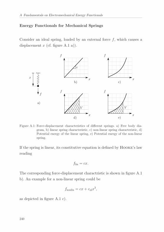
A Fundamentals on Electromechanical Energy Functionals
Energy Functionals for Mechanical Springs
Consider an ideal spring, loaded by an external force f , which causes a
displacement x (cf. figure A.1 a)).
f
x
a)
x
f
xb) c)
d) e)
f
x
f
x
f
c
V V
Figure A.1: Force-displacement characteristics of different springs. a) Free body dia-gram, b) linear spring characteristic, c) non-linear spring characteristic, d)Potential energy of the linear spring, e) Potential energy of the non-linearspring.
If the spring is linear, its constitutive equation is defined by Hooke’s law
reading
flin = cx.
The corresponding force-displacement charactristic is shown in figure A.1
b). An example for a non-linear spring could be
fnonlin = cx+ cnlx3,
as depicted in figure A.1 c).
240
The constitutive behaviour of both examples above can also be described
by an energy functional (a potential). It is introduced according to
f =dV
dx, or equivalently dV = f dx.
For the examples above, the potentials read
Vlin =1
2cx2 and Vnonlin =
1
2cx2 +
1
4cnlx
4.
In general, introducing such a potential is possible as long as the force-
displacement characteristic is energy preserving. In the end, the potential
has the same meaning as a constitutive equation here, but is expressed
in terms of energy.
Energy Functionals for Electric Capacitors
Consider an ideal capacitor, loaded by a voltage v, which causes a charge q
to accumulate (cf. figure A.2 a)). If the capacitor is linear, its constitutive
equation is defined by Coulomb’s law reading
vlin =1
Cq.
The corresponding voltage-charge characteristics is shown in figure A.2
b). An example for a non-linear capacitor could be
vnonlin =1
Cq +
1
Cnlq3,
as depicted in figure A.2 c).
241
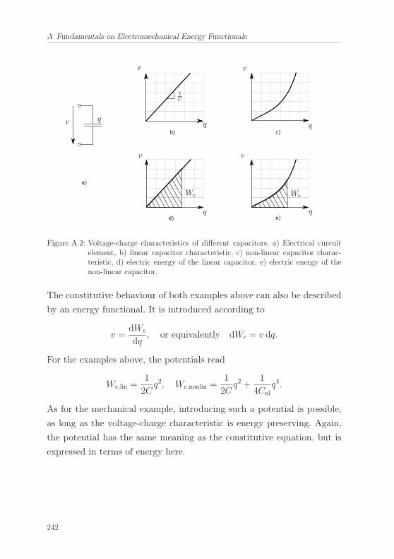
A Fundamentals on Electromechanical Energy Functionals
v v
v v
q q
1C
We We
v q
Figure A.2: Voltage-charge characteristics of different capacitors. a) Electrical curcuitelement, b) linear capacitor characteristic, c) non-linear capacitor charac-teristic, d) electric energy of the linear capacitor, e) electric energy of thenon-linear capacitor.
The constitutive behaviour of both examples above can also be described
by an energy functional. It is introduced according to
v =dWe
dq, or equivalently dWe = v dq.
For the examples above, the potentials read
We,lin =1
2Cq2, We,nonlin =
1
2Cq2 +
1
4Cnlq4.
As for the mechanical example, introducing such a potential is possible,
as long as the voltage-charge characteristic is energy preserving. Again,
the potential has the same meaning as the constitutive equation, but is
expressed in terms of energy here.
242
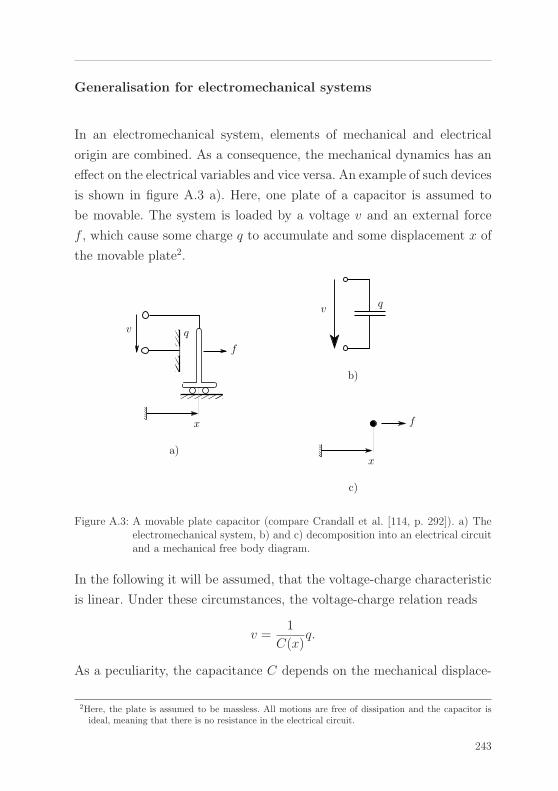
Generalisation for electromechanical systems
In an electromechanical system, elements of mechanical and electrical
origin are combined. As a consequence, the mechanical dynamics has an
effect on the electrical variables and vice versa. An example of such devices
is shown in figure A.3 a). Here, one plate of a capacitor is assumed to
be movable. The system is loaded by a voltage v and an external force
f , which cause some charge q to accumulate and some displacement x of
the movable plate2.
f
x
qv
a)
v q
x
f
b)
c)
Figure A.3: A movable plate capacitor (compare Crandall et al. [114, p. 292]). a) Theelectromechanical system, b) and c) decomposition into an electrical circuitand a mechanical free body diagram.
In the following it will be assumed, that the voltage-charge characteristic
is linear. Under these circumstances, the voltage-charge relation reads
v =1
C(x)q.
As a peculiarity, the capacitance C depends on the mechanical displace-
2Here, the plate is assumed to be massless. All motions are free of dissipation and the capacitor isideal, meaning that there is no resistance in the electrical circuit.
243
A Fundamentals on Electromechanical Energy Functionals
ment x here, as the motion changes the plate distance. In general, this
relation is non-linear, but it could be linearised, if only small motions
were to be considered.
The constitutive behaviour of this device could also be described by an
energy potential. It is defined as
v =∂We
∂q, f =
∂We
∂x, or equivalently dWe = vdq + fdx.
In contrast to the purely electrical system the energy differential in this
case has two parts. This is due to the fact, that both the charge, as well as
the mechanical displacement may alter the energy content of the system.
In the example above the electric energy reads
We =1
2C(x)q2.
Thus, the voltage and force relations are
v =1
C(x)q, f = − C ′(x)
2C(x)2q2,
where ()′ denotes the derivative with respect to x. Note, that even if 1C(x) ,
or C ′(x)2C(x)2 where linear functions with respect to x, the force-charge rela-
tion would still be non-linear. In this sense, electromechanical couplings
can be described as inherently non-linear.
As a last point it should be noted that in this example only the electrical
capacitance C has been assumed to depend on the mechanical displace-
ment x. In general, it would be possible to design a mechanical spring
with stiffness c, which would depend on the electrical charge q. In this
case the potential energy would depend both on the displacement, as well
as on the charge (V = V (x, q)). However, such an example would not be
intuitively accessible.
244
Generalisation towards multiple degrees of freedom
Commonly, technical systems are built from multiple parts and there
are multiple ways they may move. Analogously, in electrical networks,
there are multiple branches, where currents may flow and where charges
may accumulate. In such a case it is possible to gather all constitutive
equations in a single column matrix. For a mechanical system with nm
degrees of freedom, this would mean
f = f(x) ∈ Rnm×1.
In an electrical network with ne degrees of freedom, the matrix would
read
v = v(q) ∈ Rne×1.
In the case of an electromechanical system, both force and voltage are
dependent on both displacement and charge:
f = f(x, q), v = v(x, q).
If the constitutive relations can be integrated, they may be expressed in
terms of potentials. For the example of a system storing electric energy,
the potential would be defined by3
v =∂We
∂q, f =
∂We
∂x,
or equivalently
dWe = v1dq1 − ...+ vnedqne + f1dx1 − ...+ fnmdxm
= v�dq + f�dx.
Here, the partial derivative with respect to a matrix means differentiation
with respect to each component.
3For this definition, it has to be assumed, that both x and q are generalised coordinates identicallyfulfilling the kinematical contraints (compare Crandall et al. [114]).
245
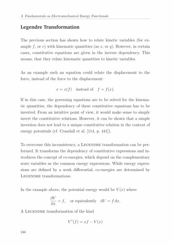
A Fundamentals on Electromechanical Energy Functionals
Legendre Transformation
The previous section has shown how to relate kinetic variables (for ex-
ample f , or v) with kinematic quantities (as x, or q). However, in certain
cases, constitutive equations are given in the inverse dependency. This
means, that they relate kinematic quantities to kinetic variables.
As an example such an equation could relate the displacement to the
force, instead of the force to the displacement:
x = x(f) instead of f = f(x).
If in this case, the governing equations are to be solved for the kinema-
tic quantities, the dependency of these constitutive equations has to be
inverted. From an intuitive point of view, it would make sense to simply
invert the constitutive relations. However, it can be shown that a simple
inversion does not lead to a unique constitutive relation in the context of
energy potentials (cf. Crandall et al. [114, p. 441]).
To overcome this inconsistency, a Legendre transformation can be per-
formed. It transforms the dependency of constitutive expressions and in-
troduces the concept of co-energies, which depend on the complementary
state variables as the common energy expressions. While energy expres-
sions are defined by a work differential, co-energies are determined by
Legendre transformations.
In the example above, the potential energy would be V (x) where
∂V
∂x= f, or equivalently dV = f dx.
A Legendre transformation of the kind
V ∗(f) = xf − V (x)
246
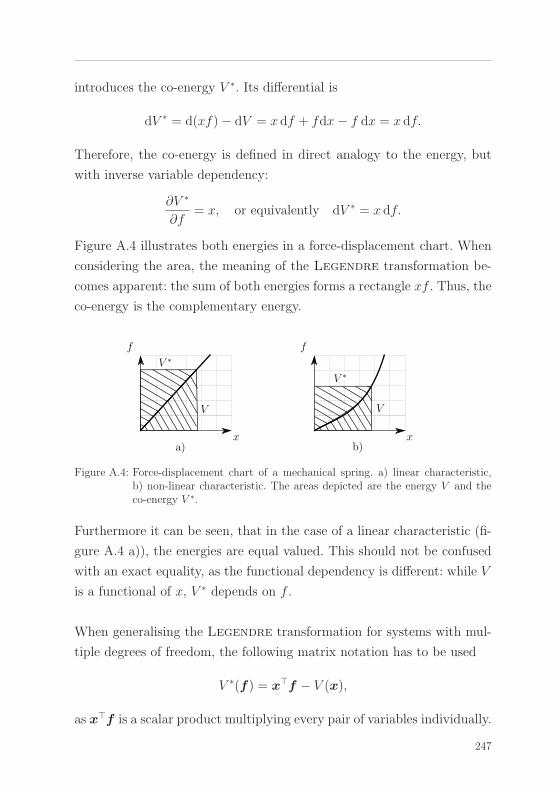
introduces the co-energy V ∗. Its differential is
dV ∗ = d(xf)− dV = x df + fdx− f dx = x df.
Therefore, the co-energy is defined in direct analogy to the energy, but
with inverse variable dependency:
∂V ∗
∂f= x, or equivalently dV ∗ = x df.
Figure A.4 illustrates both energies in a force-displacement chart. When
considering the area, the meaning of the Legendre transformation be-
comes apparent: the sum of both energies forms a rectangle xf . Thus, the
co-energy is the complementary energy.
a) b)x
f
x
f
V V
V ∗
V ∗
Figure A.4: Force-displacement chart of a mechanical spring. a) linear characteristic,b) non-linear characteristic. The areas depicted are the energy V and theco-energy V ∗.
Furthermore it can be seen, that in the case of a linear characteristic (fi-
gure A.4 a)), the energies are equal valued. This should not be confused
with an exact equality, as the functional dependency is different: while V
is a functional of x, V ∗ depends on f .
When generalising the Legendre transformation for systems with mul-
tiple degrees of freedom, the following matrix notation has to be used
V ∗(f) = x�f − V (x),
as x�f is a scalar product multiplying every pair of variables individually.
247
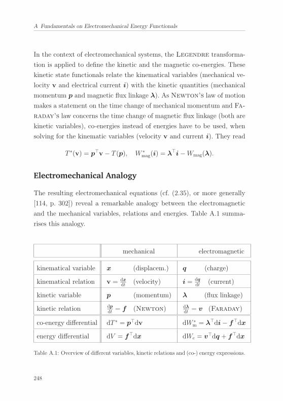
A Fundamentals on Electromechanical Energy Functionals
In the context of electromechanical systems, the Legendre transforma-
tion is applied to define the kinetic and the magnetic co-energies. These
kinetic state functionals relate the kinematical variables (mechanical ve-
locity v and electrical current i) with the kinetic quantities (mechanical
momentum p and magnetic flux linkage λ). As Newton’s law of motion
makes a statement on the time change of mechanical momentum and Fa-
raday’s law concerns the time change of magnetic flux linkage (both are
kinetic variables), co-energies instead of energies have to be used, when
solving for the kinematic variables (velocity v and current i). They read
T ∗(v) = p�v − T (p), W ∗mag(i) = λ�i−Wmag(λ).
Electromechanical Analogy
The resulting electromechanical equations (cf. (2.35), or more generally
[114, p. 302]) reveal a remarkable analogy between the electromagnetic
and the mechanical variables, relations and energies. Table A.1 summa-
rises this analogy.
mechanical electromagnetic
kinematical variable x (displacem.) q (charge)
kinematical relation v = dxdt (velocity) i = dq
dt (current)
kinetic variable p (momentum) λ (flux linkage)
kinetic relation dpdt = f (Newton) dλ
dt = v (Faraday)
co-energy differential dT ∗ = p�dv dW ∗m = λ�di− f�dx
energy differential dV = f�dx dWe = v�dq + f�dx
Table A.1: Overview of different variables, kinetic relations and (co-) energy expressions.
248
B Asymptotic Expansion of theAir-Gap Magnetic Field
Within this chapter, the magnetic field problem in the air-gap will be
solved approximately using an asymptotic expansion. This approach is
described in more detail in [48] and will be summarised here1.
Starting from the field equation, defined in (2.81) and considering the
boundary conditions (2.77), the problem to solve reads
ΔF = 0 in Ωδ (B.1)
subject to the boundary conditions
�n× �h
∣∣∣∣Γδ1
= �n× �he1 on Γδ1, (B.2a)
�n× �h
∣∣∣∣Γδ2
= �n× �he2 on Γδ2. (B.2b)
Here, the vectors �he1 and �he2 are the magnetic field in the stator and
rotor, adjacent to the air-gap, respectively. They are considered as given
boundary condition for this derivation.
In order to expand the potential asymptotically, a small parameter has
to be identified. To this end, consider the definition of the radius to the
rotor surface R2δ, as defined in (2.80). When relating it to the rotor radius
1For the sake of consistency with this thesis, there are some differences in notation compared to [48].
249
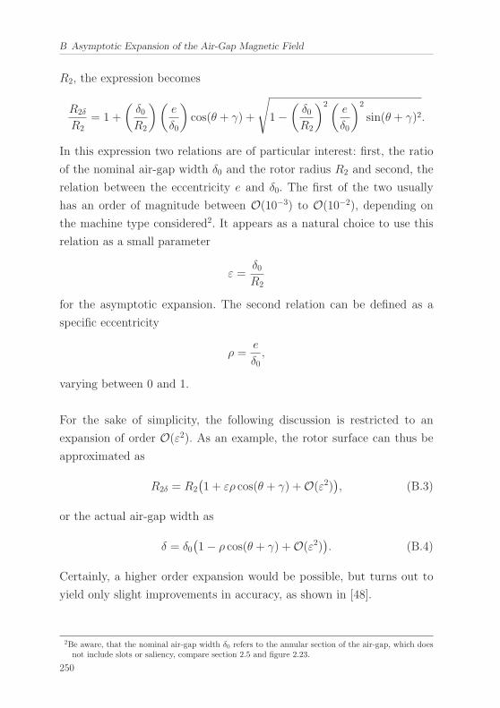
B Asymptotic Expansion of the Air-Gap Magnetic Field
R2, the expression becomes
R2δ
R2= 1 +
(δ0R2
)(e
δ0
)cos(θ + γ) +
√1−(δ0R2
)2(e
δ0
)2
sin(θ + γ)2.
In this expression two relations are of particular interest: first, the ratio
of the nominal air-gap width δ0 and the rotor radius R2 and second, the
relation between the eccentricity e and δ0. The first of the two usually
has an order of magnitude between O(10−3) to O(10−2), depending on
the machine type considered2. It appears as a natural choice to use this
relation as a small parameter
ε =δ0R2
for the asymptotic expansion. The second relation can be defined as a
specific eccentricity
ρ =e
δ0,
varying between 0 and 1.
For the sake of simplicity, the following discussion is restricted to an
expansion of order O(ε2). As an example, the rotor surface can thus be
approximated as
R2δ = R2
(1 + ερ cos(θ + γ) +O(ε2)
), (B.3)
or the actual air-gap width as
δ = δ0(1− ρ cos(θ + γ) +O(ε2)
). (B.4)
Certainly, a higher order expansion would be possible, but turns out to
yield only slight improvements in accuracy, as shown in [48].
2Be aware, that the nominal air-gap width δ0 refers to the annular section of the air-gap, which doesnot include slots or saliency, compare section 2.5 and figure 2.23.
250
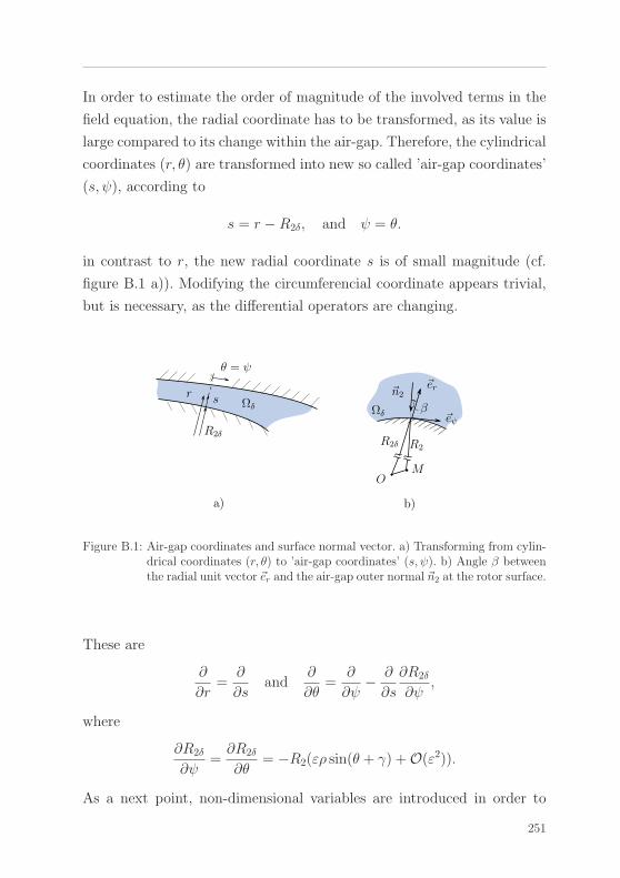
In order to estimate the order of magnitude of the involved terms in the
field equation, the radial coordinate has to be transformed, as its value is
large compared to its change within the air-gap. Therefore, the cylindrical
coordinates (r, θ) are transformed into new so called ’air-gap coordinates’
(s, ψ), according to
s = r −R2δ, and ψ = θ.
in contrast to r, the new radial coordinate s is of small magnitude (cf.
figure B.1 a)). Modifying the circumferencial coordinate appears trivial,
but is necessary, as the differential operators are changing.
R2δ
s
θ = ψ
Ωδ
�n2�er
β�eψ
MO
R2δ R2
a) b)
r
Ωδ
Figure B.1: Air-gap coordinates and surface normal vector. a) Transforming from cylin-drical coordinates (r, θ) to ’air-gap coordinates’ (s, ψ). b) Angle β betweenthe radial unit vector �er and the air-gap outer normal �n2 at the rotor surface.
These are
∂
∂r=
∂
∂sand
∂
∂θ=
∂
∂ψ− ∂
∂s
∂R2δ
∂ψ,
where
∂R2δ
∂ψ=∂R2δ
∂θ= −R2(ερ sin(θ + γ) +O(ε2)).
As a next point, non-dimensional variables are introduced in order to
251
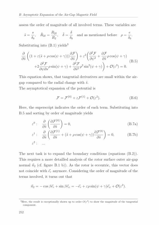
B Asymptotic Expansion of the Air-Gap Magnetic Field
assess the order of magnitude of all involved terms. These variables are
s =s
δ0, R2δ =
R2δ
R2, δ =
δ
δ0and as mentioned before ρ =
e
δ0.
Substituting into (B.1) yields3
∂
∂s
((1 + ε(s+ ρ cos(ψ + γ)))
∂F∂s
)+ ε2
(∂2F∂ψ2
+∂F∂s
ρ cos(ψ + γ)
+2∂2F∂ψ∂s
ρ sin(ψ + γ) +∂2F∂s2
ρ2 sin2(ψ + γ)
)+O(ε3) = 0.
(B.5)
This equation shows, that tangential derivatives are small within the air-
gap compared to the radial change with s.
The asymptotical expansion of the potential is
F = F{0} + εF{1} +O(ε2). (B.6)
Here, the superscript indicates the order of each term. Substituting into
B.5 and sorting by order of magnitude yields
ε0 :∂
∂s
(∂F{0}
∂s
)= 0, (B.7a)
ε1 :∂
∂s
(∂F{1}
∂s+ (s+ ρ cos(ψ + γ))
∂F (0)
∂s
)= 0, (B.7b)
ε2 : ...
The next task is to expand the boundary conditions (equations (B.2)).
This requires a more detailled analysis of the rotor surface outer air-gap
normal �n2 (cf. figure B.1 b)). As the rotor is eccentric, this vector does
not coincide with �er anymore. Considering the order of magnitude of the
terms involved, it turns out that
�n2 = − cos β�er + sin β�eψ = −�er + ερ sin(ψ + γ)�eψ +O(ε2).
3Here, the result is exceptionally shown up to order O(ε2) to show the magnitude of the tangentialcomponent.
252
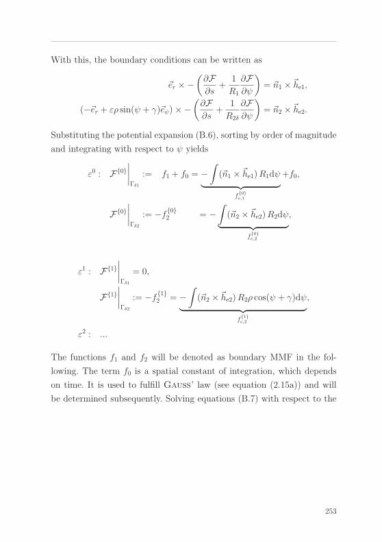
With this, the boundary conditions can be written as
�er ×−(∂F∂s
+1
R1
∂F∂ψ
)= �n1 × �he1,
(−�er + ερ sin(ψ + γ)�eψ)×−(∂F∂s
+1
R2δ
∂F∂ψ
)= �n2 × �he2.
Substituting the potential expansion (B.6), sorting by order of magnitude
and integrating with respect to ψ yields
ε0 : F{0}∣∣∣∣Γδ1
:= f1 + f0 = −∫
(�n1 × �he1)R1dψ︸ ︷︷ ︸f{0}e,1
+f0,
F{0}∣∣∣∣Γδ2
:= −f {0}2 = −∫
(�n2 × �he2)R2dψ︸ ︷︷ ︸f{0}e,2
,
ε1 : F{1}∣∣∣∣Γδ1
= 0,
F{1}∣∣∣∣Γδ2
:= −f {1}2 = −∫
(�n2 × �he2)R2ρ cos(ψ + γ)dψ︸ ︷︷ ︸f{1}e,2
,
ε2 : ...
The functions f1 and f2 will be denoted as boundary MMF in the fol-
lowing. The term f0 is a spatial constant of integration, which depends
on time. It is used to fulfill Gauss’ law (see equation (2.15a)) and will
be determined subsequently. Solving equations (B.7) with respect to the
253
B Asymptotic Expansion of the Air-Gap Magnetic Field
expanded boundary conditions results in
ε0 : F{0} = −(f1 + f{0}2
) s
δ{0}+ f
{0}2 , (B.8)
ε1 : F{1}1 = − δ
{0}
2
(1− 2
δ{1}
(δ{0})2− s
δ{0}
)(f1 + f
{0}2
) s
δ{0}
+
(1− s
δ{0}
)f{1}2 , (B.9)
ε2 : ...
The flux density can be found by calculating the gradient of F . It reads
ε0 : �b{0} = b{0}s �es + b
{0}ψ �eψ, (B.10)
b{0}s =
μ0δ0
1
δ{0}(f1 + f
{0}2 ), b
{0}ψ = 0.
ε1 : �b{1} = b{1}s �es + b
{1}ψ �eψ, (B.11)
b{1}s = −μ0
δ0
∂F{1}
∂s, b
{1}ψ = −μ0
δ0
(∂F{0}
∂ψ+∂F{0}
∂sρ sinψ
).
ε2 ...
where the terms ∂F{1}∂s , ∂F
{0}∂ψ and ∂F{0}
∂s are not stated explicitly for the
sake of shortness. From this results, it can be seen, that the tangential
field component bψ is one order of magnitude smaller than the radial part
bs (as b{0}ψ = 0). Although it seems reasonable to neglect the tangential
component due to its small magnitude compared to the radial component
in the first place, this is not permissible in general. For example, neglecting
the tangential component in the torque expression would result in a zero
solution. Moreover, the boundary conditions cannot be met without a
tangential part in the field vector. Therefore, this component can only be
neglected if there is a larger term in the same mathematical expression,
for example in the magnetic force.
254
Returning to the dimensional form and regarding only first order appro-
ximations, the following field solution is obtained from the asymptotic
approximation:
F = −(f1 + f2)r −R2δ
δ+ f2, �b = br�er + bθ�eθ, (B.12a)
where
br =μ0δ
(f1 + f2
), bθ = −μ0
R
(∂(f1 + f2)
∂θ
(r −R2δ
δ
)− ∂f2
∂θ
). (B.12b)
Here, the only question left is how to determine the spatial constant of
integration f0(t). It can be answered, by integratingGauß’ law (equation
(2.15a)) over the stator bore surface:
0 = �
∮�b · �n dA
= �R1
∫ π
−πbr dθ
= �R1
∫ π
−π
μ0δ
(f1 + f2
)dθ
= �R1
∫ π
−π
μ0δ
(fe,1 + f0 + fe,2
)dθ.
In the end, solving for f0(t) yields
f0 = −∫ π−π
μ0
δ (fe1 + fe2) �R1dθ∫ π−π
μ0
δ �R1dθ. (B.13)
Having defined the field solution, the electromechanical coupling can be
defined. It can be calculated either directly using equations (2.28), or
indirectly from the magnetic (co-)energy, as defined in (2.38). For the
derivation and for showing the equivalence of both approaches (section
2.6.3) an intermediate radius R = R1+R2
2 has been introduced. Using this
255

B Asymptotic Expansion of the Air-Gap Magnetic Field
simplification can be justified in the following manner
R1 = R +δ02
= R
(1 +
1
2
R2
R
δ0R2︸︷︷︸=ε
)= R +O(ε), (B.14a)
R2 = R− δ02
= R
(1− 1
2
R2
R
δ0R2︸︷︷︸=ε
)= R +O(ε). (B.14b)
From this consideration it can be seen that the error involved when re-
garding the air-gap as a one dimensional line of radius R is small (order
O(ε)).
The last point to address within this section is the choice of a scalar ma-
gnetic potential instead of a vector potential for the field solution (compa-
re equations (2.75)). The reason for this lies in the result of the asymptotic
approximation. As it can be seen from equations (B.12), the approxima-
tion based on a scalar potential results in a flux density, which has a
radially constant component br and a tangential part bθ, which is linear
in the radial coordinate. In contrast to that, an approximative solution
based on a vector potential results in a radially constant component bθ
and a radial part br, which is linear in the radial coordinate. The pro-
blem in this latter case is, that such an approximation cannot fulfil the
boundary conditions for the tangential field component, as there are two
different boundary functions for just one constant solution component.
Therefore, a vector potential is not suited to be used for an asymptotic
approximation of the air-gap field problem.
256
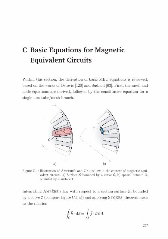
C Basic Equations for MagneticEquivalent Circuits
Within this section, the derivation of basic MEC equations is reviewed,
based on the works of Ostovic [120] and Sudhoff [63]. First, the mesh and
node equations are derived, followed by the constitutive equation for a
single flux tube/mesh branch.
b)a)
C
S ΩΓ
Figure C.1: Illustration of Ampere’s and Gauß’ law in the context of magnetic equi-valent circuits. a) Surface S bounded by a curve C, b) spatial domain Ω,bounded by a surface Γ.
Integrating Ampere’s law with respect to a certain surface S, boundedby a curve C (compare figure C.1 a)) and applying Stokes’ theorem leads
to the relation ∮C�h · d�s =
∫S�j · �n dA.
257
C Basic Equations for Magnetic Equivalent Circuits
When subdividing the curve into sections Ck(k = 1, ..., nm) and defining∫Ck�h · d�s = Fk, and
∫S�j · �n dA = Fs, (C.1)
this area can be considered as a mesh of a network, analogously to the
definition of Kirchhoff for electrical networks leading to the mesh equa-
tion
nm∑k=1
Fk = Fs. (C.2)
In this context, ΔFk is commonly denoted as MMF drop1, while Fs is an
MMF source (current linkage).
When integrating Gauß’ law with respect to a certain spatial domain
Ω bounded by a surface Γ (compare figure C.1 b)) and applying Gauß’
theorem, the relation ∮Γ
�b · �n dA = 0
is found. When subdividing the surface into sections Γk, (k = 1, ..., nn)
and defining ∫Γk
�b · �n dA = Φk, (C.3)
this volume can be considered as a node of a network, again analogously
to the definition of Kirchhoff leading to the node equation
nn∑k=1
Φk = 0. (C.4)
1Compared to the definition of the magneto-motive force in the air-gap domain, it is important tonote, that the MMF in these equations is not associated to a mangnetic potential.
258
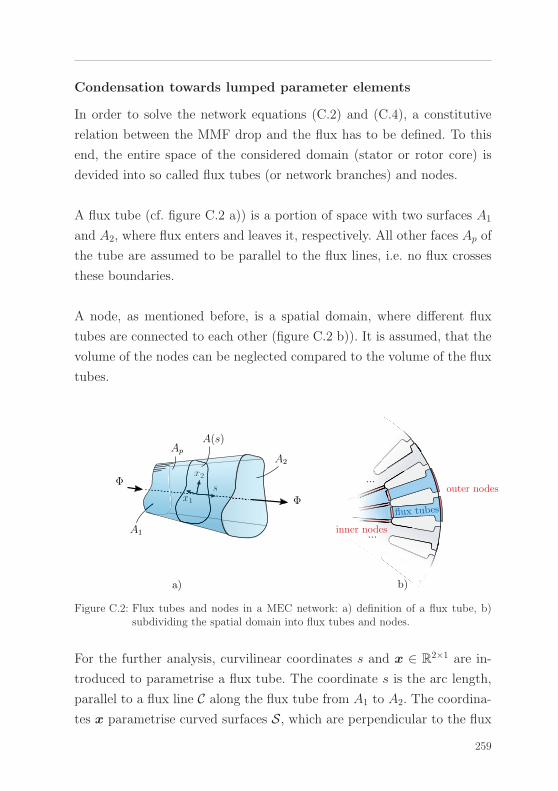
Condensation towards lumped parameter elements
In order to solve the network equations (C.2) and (C.4), a constitutive
relation between the MMF drop and the flux has to be defined. To this
end, the entire space of the considered domain (stator or rotor core) is
devided into so called flux tubes (or network branches) and nodes.
A flux tube (cf. figure C.2 a)) is a portion of space with two surfaces A1
and A2, where flux enters and leaves it, respectively. All other faces Ap of
the tube are assumed to be parallel to the flux lines, i.e. no flux crosses
these boundaries.
A node, as mentioned before, is a spatial domain, where different flux
tubes are connected to each other (figure C.2 b)). It is assumed, that the
volume of the nodes can be neglected compared to the volume of the flux
tubes.
a) b)
x1s
x2
xxx111ss
xx2Φ
A1
A2
A(s)Ap
Φ
...
flux tubes
outer nodes
inner nodes...
Figure C.2: Flux tubes and nodes in a MEC network: a) definition of a flux tube, b)subdividing the spatial domain into flux tubes and nodes.
For the further analysis, curvilinear coordinates s and x ∈ R2×1 are in-
troduced to parametrise a flux tube. The coordinate s is the arc length,
parallel to a flux line C along the flux tube from A1 to A2. The coordina-
tes x parametrise curved surfaces S, which are perpendicular to the flux
259
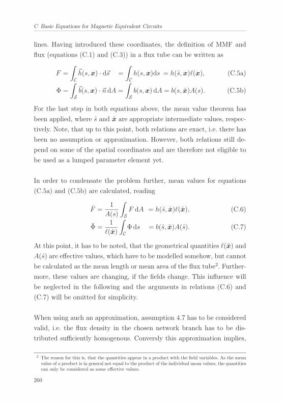
C Basic Equations for Magnetic Equivalent Circuits
lines. Having introduced these coordinates, the definition of MMF and
flux (equations (C.1) and (C.3)) in a flux tube can be written as
F =
∫C�h(s,x) · d�s =
∫Ch(s,x)ds = h(s,x)�(x), (C.5a)
Φ =
∫S�b(s,x) · �n dA =
∫Sb(s,x) dA = b(s, x)A(s). (C.5b)
For the last step in both equations above, the mean value theorem has
been applied, where s and x are appropriate intermediate values, respec-
tively. Note, that up to this point, both relations are exact, i.e. there has
been no assumption or approximation. However, both relations still de-
pend on some of the spatial coordinates and are therefore not eligible to
be used as a lumped parameter element yet.
In order to condensate the problem further, mean values for equations
(C.5a) and (C.5b) are calculated, reading
F =1
A(s)
∫SF dA = h(s, x)�(x), (C.6)
Φ =1
�(x)
∫CΦds = b(s, x)A(s). (C.7)
At this point, it has to be noted, that the geometrical quantities �(x) and
A(s) are effective values, which have to be modelled somehow, but cannot
be calculated as the mean length or mean area of the flux tube2. Further-
more, these values are changing, if the fields change. This influence will
be neglected in the following and the arguments in relations (C.6) and
(C.7) will be omitted for simplicity.
When using auch an approximation, assumption 4.7 has to be considered
valid, i.e. the flux density in the chosen network branch has to be dis-
tributed sufficiently homogenous. Conversly this approximation implies,
2 The reason for this is, that the quantities appear in a product with the field variables. As the meanvalue of a product is in general not equal to the product of the individual mean values, the quantitiescan only be considered as some effective values.
260
that flux concentrations e.g. at an edge cannot be modelled anymore. Ho-
wever, as for the problems considered in this work, such inhomogenities
play a minor role, the approximation gives accurate results, as it will be
verified in chapter 3.
As a last step, the material behaviour has to be introduced, linking b and
h. It can be written in the general form
b = bM(h) + bR, or h = hM(b− bR), (C.8)
if assumptions 4.8 and 4.9 hold, i.e. if the constitutive equation can be
considered isotropic and the remanent flux density bR is constant. Here,
bM and hM represent the magnetisation curve.
Substituting relations (C.8) in (C.6), or (C.7), respectively and expressing
b and h in terms of F and Φ yields
F = hM
(Φ− ΦR
A
)�, (C.9)
Φ = bM
(ΔF
�
)A+ ΦR. (C.10)
At the end, equations (C.2) and (C.4), together with one of the constitu-
tive relations (C.9), or (C.10) form the basic MEC equations.
261
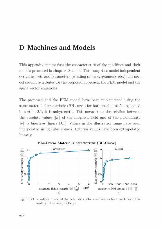
D Machines and Models
This appendix summarises the characteristics of the machines and their
models presented in chapters 3 and 4. This comprises model independent
design aspects and parameters (winding scheme, geometry etc.) and mo-
del specific attributes for the proposed approach, the FEM model and the
space vector equations.
The proposed and the FEM model have been implemented using the
same material characteristic (BH-curve) for both machines. As explained
in section 2.1, it is anhysteretic. This means that the relation between
the absolute values ‖�h‖ of the magnetic field and of the flux density
‖�b‖ is bijective (figure D.1). Values in the illustrated range have been
interpolated using cubic splines. Exterior values have been extrapolated
linearly.
Figure D.1: Non-linear material characteristic (BH-curve) used for both machines in thiswork. a) Overview, b) Detail.
262
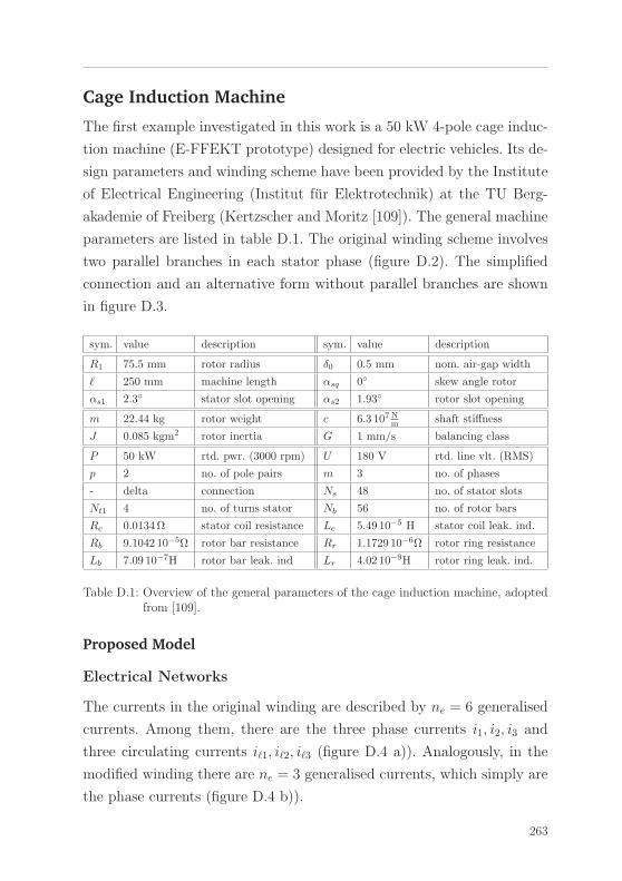
Cage Induction Machine
The first example investigated in this work is a 50 kW 4-pole cage induc-
tion machine (E-FFEKT prototype) designed for electric vehicles. Its de-
sign parameters and winding scheme have been provided by the Institute
of Electrical Engineering (Institut fur Elektrotechnik) at the TU Berg-
akademie of Freiberg (Kertzscher and Moritz [109]). The general machine
parameters are listed in table D.1. The original winding scheme involves
two parallel branches in each stator phase (figure D.2). The simplified
connection and an alternative form without parallel branches are shown
in figure D.3.
sym. value description sym. value description
R1 75.5 mm rotor radius δ0 0.5 mm nom. air-gap width
� 250 mm machine length αsq 0◦ skew angle rotor
αs1 2.3◦ stator slot opening αs2 1.93◦ rotor slot opening
m 22.44 kg rotor weight c 6.3 107 Nm shaft stiffness
J 0.085 kgm2 rotor inertia G 1 mm/s balancing class
P 50 kW rtd. pwr. (3000 rpm) U 180 V rtd. line vlt. (RMS)
p 2 no. of pole pairs m 3 no. of phases
- delta connection Ns 48 no. of stator slots
Nt1 4 no. of turns stator Nb 56 no. of rotor bars
Rc 0.0134Ω stator coil resistance Lc 5.49 10−5 H stator coil leak. ind.
Rb 9.1042 10−5Ω rotor bar resistance Rr 1.1729 10−6Ω rotor ring resistance
Lb 7.09 10−7H rotor bar leak. ind Lr 4.02 10−9H rotor ring leak. ind.
Table D.1: Overview of the general parameters of the cage induction machine, adoptedfrom [109].
Proposed Model
Electrical Networks
The currents in the original winding are described by ne = 6 generalised
currents. Among them, there are the three phase currents i1, i2, i3 and
three circulating currents i�1, i�2, i�3 (figure D.4 a)). Analogously, in the
modified winding there are ne = 3 generalised currents, which simply are
the phase currents (figure D.4 b)).
263
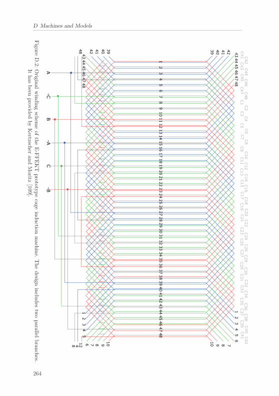
D Machines and Models
Figu
reD.2:
Origin
alwindingsch
emeof
theE-FFEKT
prototy
pecage
induction
mach
ine.
Thedesign
inclu
des
twoparallel
bran
ches.
Ithas
been
prov
ided
byKertzsch
eran
dMoritz
[109].
264
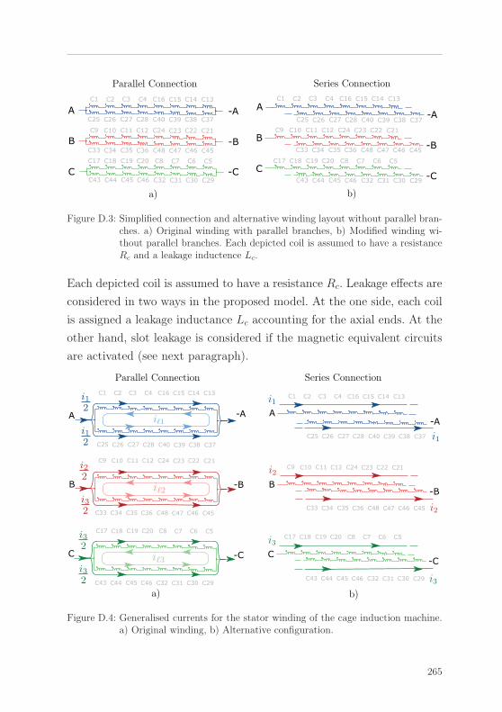
a)
Parallel Connection Series Connection
b)
Figure D.3: Simplified connection and alternative winding layout without parallel bran-ches. a) Original winding with parallel branches, b) Modified winding wi-thout parallel branches. Each depicted coil is assumed to have a resistanceRc and a leakage inductence Lc.
Each depicted coil is assumed to have a resistance Rc. Leakage effects are
considered in two ways in the proposed model. At the one side, each coil
is assigned a leakage inductance Lc accounting for the axial ends. At the
other hand, slot leakage is considered if the magnetic equivalent circuits
are activated (see next paragraph).
i1
i12
i12
i2
i22
i32
i3
i32
i32
Series Connection
b)
Parallel Connection
a)
i1
i1
i2
i2
i3
i3
Figure D.4: Generalised currents for the stator winding of the cage induction machine.a) Original winding, b) Alternative configuration.
265
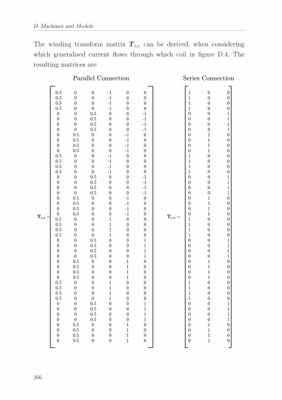
D Machines and Models
The winding transform matrix T c,e can be derived, when considering
which generalised current flows through which coil in figure D.4. The
resulting matrices are
266
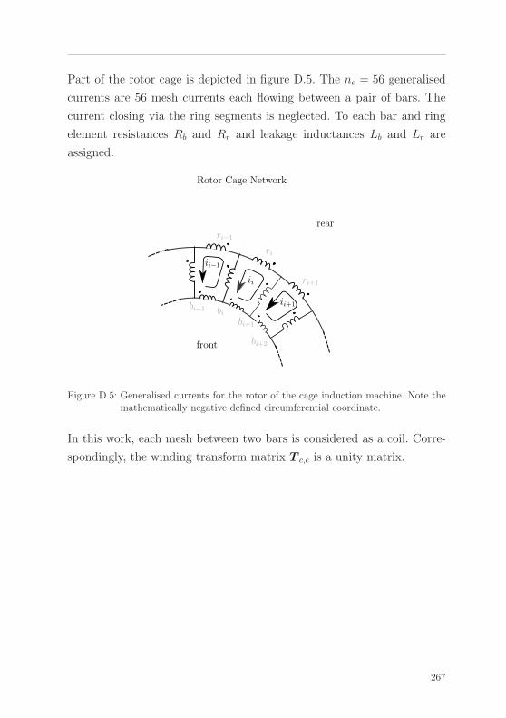
Part of the rotor cage is depicted in figure D.5. The ne = 56 generalised
currents are 56 mesh currents each flowing between a pair of bars. The
current closing via the ring segments is neglected. To each bar and ring
element resistances Rb and Rr and leakage inductances Lb and Lr are
assigned.
Rotor Cage Network
front
rear
ii
ii+1
ii−1
bi+1
bibi−1
bi+2
ri
ri−1
ri+1
Figure D.5: Generalised currents for the rotor of the cage induction machine. Note themathematically negative defined circumferential coordinate.
In this work, each mesh between two bars is considered as a coil. Corre-
spondingly, the winding transform matrix T c,e is a unity matrix.
267
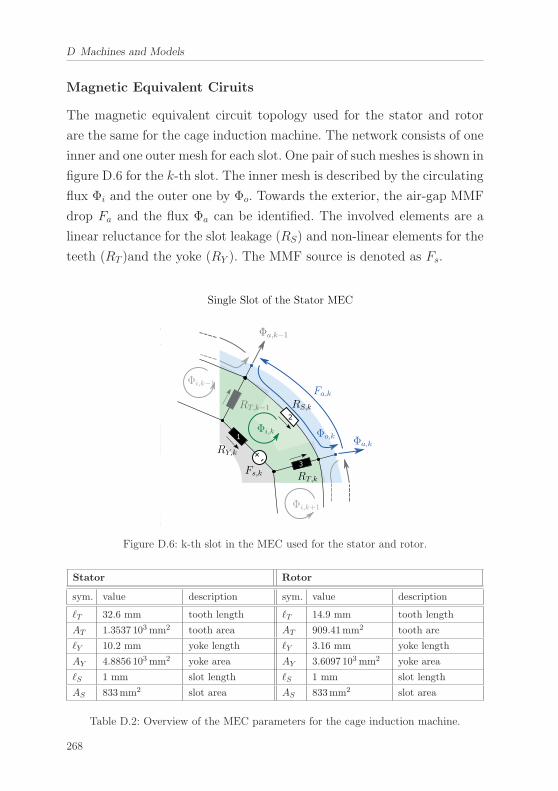
D Machines and Models
Magnetic Equivalent Ciruits
The magnetic equivalent circuit topology used for the stator and rotor
are the same for the cage induction machine. The network consists of one
inner and one outer mesh for each slot. One pair of such meshes is shown in
figure D.6 for the k-th slot. The inner mesh is described by the circulating
flux Φi and the outer one by Φo. Towards the exterior, the air-gap MMF
drop Fa and the flux Φa can be identified. The involved elements are a
linear reluctance for the slot leakage (RS) and non-linear elements for the
teeth (RT )and the yoke (RY ). The MMF source is denoted as Fs.
Fs,k
Fa,k
Φa,k
Φa,k−1
Φo,kΦi,k
Φi,k−1
RY,k
RT,k−1
RT,k
RS,k
Single Slot of the Stator MEC
Φi,k+1
Figure D.6: k-th slot in the MEC used for the stator and rotor.
Stator Rotor
sym. value description sym. value description
�T 32.6 mm tooth length �T 14.9 mm tooth length
AT 1.3537 103mm2 tooth area AT 909.41mm2 tooth are
�Y 10.2 mm yoke length �Y 3.16 mm yoke length
AY 4.8856 103mm2 yoke area AY 3.6097 103mm2 yoke area
�S 1 mm slot length �S 1 mm slot length
AS 833mm2 slot area AS 833mm2 slot area
Table D.2: Overview of the MEC parameters for the cage induction machine.
268
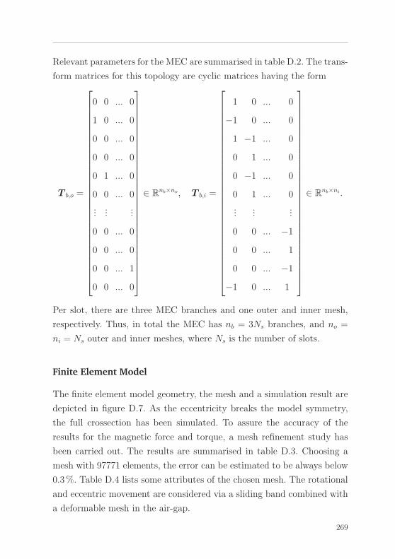
Relevant parameters for the MEC are summarised in table D.2. The trans-
form matrices for this topology are cyclic matrices having the form
T b,o =
⎡⎢⎢⎢⎢⎢⎢⎢⎢⎢⎢⎢⎢⎢⎢⎢⎢⎢⎢⎢⎢⎢⎢⎢⎢⎢⎢⎢⎢⎢⎢⎣
0 0 ... 0
1 0 ... 0
0 0 ... 0
0 0 ... 0
0 1 ... 0
0 0 ... 0
......
...
0 0 ... 0
0 0 ... 0
0 0 ... 1
0 0 ... 0
⎤⎥⎥⎥⎥⎥⎥⎥⎥⎥⎥⎥⎥⎥⎥⎥⎥⎥⎥⎥⎥⎥⎥⎥⎥⎥⎥⎥⎥⎥⎥⎦
∈ Rnb×no, T b,i =
⎡⎢⎢⎢⎢⎢⎢⎢⎢⎢⎢⎢⎢⎢⎢⎢⎢⎢⎢⎢⎢⎢⎢⎢⎢⎢⎢⎢⎢⎢⎢⎣
1 0 ... 0
−1 0 ... 0
1 −1 ... 0
0 1 ... 0
0 −1 ... 0
0 1 ... 0
......
...
0 0 ... −1
0 0 ... 1
0 0 ... −1
−1 0 ... 1
⎤⎥⎥⎥⎥⎥⎥⎥⎥⎥⎥⎥⎥⎥⎥⎥⎥⎥⎥⎥⎥⎥⎥⎥⎥⎥⎥⎥⎥⎥⎥⎦
∈ Rnb×ni.
Per slot, there are three MEC branches and one outer and inner mesh,
respectively. Thus, in total the MEC has nb = 3Ns branches, and no =
ni = Ns outer and inner meshes, where Ns is the number of slots.
Finite Element Model
The finite element model geometry, the mesh and a simulation result are
depicted in figure D.7. As the eccentricity breaks the model symmetry,
the full crossection has been simulated. To assure the accuracy of the
results for the magnetic force and torque, a mesh refinement study has
been carried out. The results are summarised in table D.3. Choosing a
mesh with 97771 elements, the error can be estimated to be always below
0.3%. Table D.4 lists some attributes of the chosen mesh. The rotational
and eccentric movement are considered via a sliding band combined with
a deformable mesh in the air-gap.
269
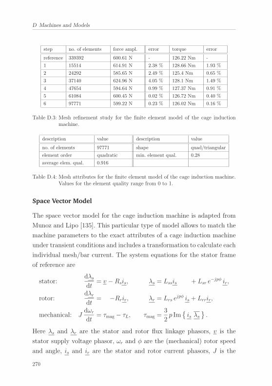
D Machines and Models
step no. of elements force ampl. error torque error
reference 339392 600.61 N - 126.22 Nm -
1 15514 614.91 N 2.38 % 128.66 Nm 1.93 %
2 24292 585.65 N 2.49 % 125.4 Nm 0.65 %
3 37140 624.96 N 4.05 % 128.1 Nm 1.49 %
4 47654 594.64 N 0.99 % 127.37 Nm 0.91 %
5 61084 600.45 N 0.02 % 126.72 Nm 0.40 %
6 97771 599.22 N 0.23 % 126.02 Nm 0.16 %
Table D.3: Mesh refinement study for the finite element model of the cage inductionmachine.
description value description value
no. of elements 97771 shape quad/triangular
element order quadratic min. element qual. 0.28
average elem. qual. 0.916
Table D.4: Mesh attributes for the finite element model of the cage induction machine.Values for the element quality range from 0 to 1.
Space Vector Model
The space vector model for the cage induction machine is adapted from
Munoz and Lipo [135]. This particular type of model allows to match the
machine parameters to the exact attributes of a cage induction machine
under transient conditions and includes a transformation to calculate each
individual mesh/bar current. The system equations for the stator frame
of reference are
stator:dλs
dt= v −Rsis, λs = Lssis + Lsr e
−jpφ ir,
rotor:dλr
dt= −Rrir, λr = Lrs e
jpφ is + Lrrir,
mechanical: Jdωrdt
= τmag − τL, τmag =3
2p Im
{is λs
}.
Here λs and λr are the stator and rotor flux linkage phasors, v is the
stator supply voltage phasor, ωr and φ are the (mechanical) rotor speed
and angle, is and ir are the stator and rotor current phasors, J is the
270
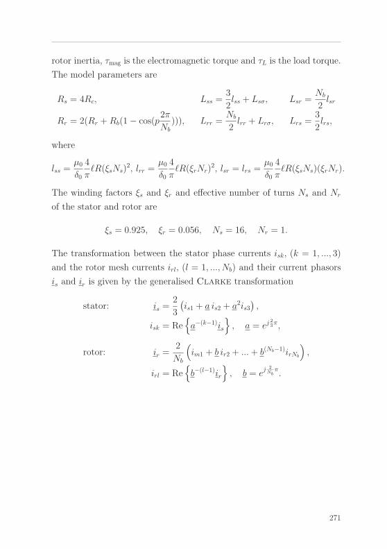
rotor inertia, τmag is the electromagnetic torque and τL is the load torque.
The model parameters are
Rs = 4Rc, Lss =3
2lss + Lsσ, Lsr =
Nb
2lsr
Rr = 2(Rr +Rb(1− cos(p2π
Nb))), Lrr =
Nb
2lrr + Lrσ, Lrs =
3
2lrs,
where
lss =μ0δ0
4
π�R(ξsNs)
2, lrr =μ0δ0
4
π�R(ξrNr)
2, lsr = lrs =μ0δ0
4
π�R(ξsNs)(ξrNr).
The winding factors ξs and ξr and effective number of turns Ns and Nr
of the stator and rotor are
ξs = 0.925, ξr = 0.056, Ns = 16, Nr = 1.
The transformation between the stator phase currents isk, (k = 1, ..., 3)
and the rotor mesh currents irl, (l = 1, ..., Nb) and their current phasors
is and ir is given by the generalised Clarke transformation
stator: is =2
3
(is1 + a is2 + a2is3
),
isk = Re{a−(k−1)is
}, a = ej
23π,
rotor: ir =2
Nb
(im1 + b ir2 + ...+ b(Nb−1)irNb
),
irl = Re{b−(l−1)ir
}, b = e
j 2Nbπ.
271
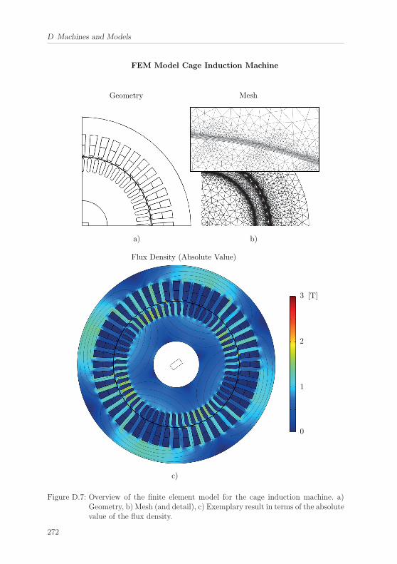
D Machines and Models
a) b)
c)
Geometry Mesh
Flux Density (Absolute Value)
[T]3
2
1
0
FEM Model Cage Induction Machine
Figure D.7: Overview of the finite element model for the cage induction machine. a)Geometry, b) Mesh (and detail), c) Exemplary result in terms of the absolutevalue of the flux density.
272
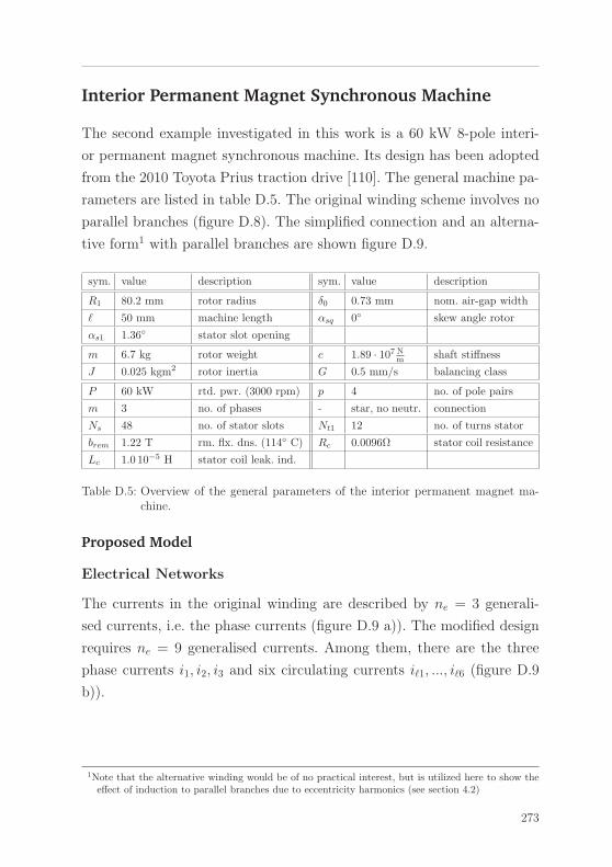
Interior Permanent Magnet Synchronous Machine
The second example investigated in this work is a 60 kW 8-pole interi-
or permanent magnet synchronous machine. Its design has been adopted
from the 2010 Toyota Prius traction drive [110]. The general machine pa-
rameters are listed in table D.5. The original winding scheme involves no
parallel branches (figure D.8). The simplified connection and an alterna-
tive form1 with parallel branches are shown figure D.9.
sym. value description sym. value description
R1 80.2 mm rotor radius δ0 0.73 mm nom. air-gap width
� 50 mm machine length αsq 0◦ skew angle rotor
αs1 1.36◦ stator slot opening
m 6.7 kg rotor weight c 1.89 · 107 Nm shaft stiffness
J 0.025 kgm2 rotor inertia G 0.5 mm/s balancing class
P 60 kW rtd. pwr. (3000 rpm) p 4 no. of pole pairs
m 3 no. of phases - star, no neutr. connection
Ns 48 no. of stator slots Nt1 12 no. of turns stator
brem 1.22 T rm. flx. dns. (114◦ C) Rc 0.0096Ω stator coil resistance
Lc 1.0 10−5 H stator coil leak. ind.
Table D.5: Overview of the general parameters of the interior permanent magnet ma-chine.
Proposed Model
Electrical Networks
The currents in the original winding are described by ne = 3 generali-
sed currents, i.e. the phase currents (figure D.9 a)). The modified design
requires ne = 9 generalised currents. Among them, there are the three
phase currents i1, i2, i3 and six circulating currents i�1, ..., i�6 (figure D.9
b)).
1Note that the alternative winding would be of no practical interest, but is utilized here to show theeffect of induction to parallel branches due to eccentricity harmonics (see section 4.2)
273
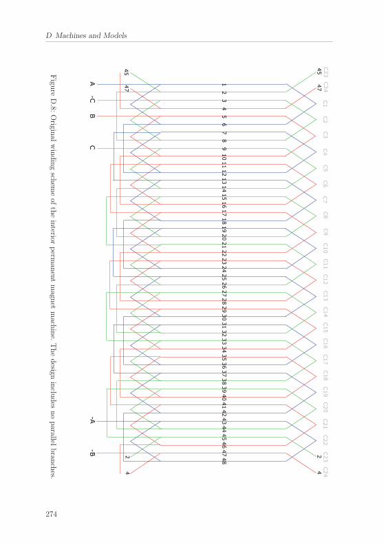
D Machines and Models
Figu
reD.8:
Origin
alwindingsch
emeof
theinterior
perm
anentmagn
etmach
ine.
Thedesign
inclu
des
noparallel
bran
ches.
274
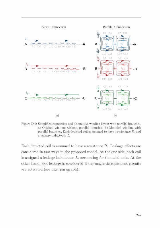
b)
Parallel ConnectionSeries Connection
a)
i1
i2
i3
i12
i12
i22
i32
i32
i32
i1 i2
i3 i4
i5 i6
Figure D.9: Simplified connection and alternative winding layout with parallel branches.a) Original winding without parallel branches, b) Modified winding withparallel branches. Each depicted coil is assumed to have a resistance Rc anda leakage inductence Lc.
Each depicted coil is assumed to have a resistance Rc. Leakage effects are
considered in two ways in the proposed model. At the one side, each coil
is assigned a leakage inductance Lc accounting for the axial ends. At the
other hand, slot leakage is considered if the magnetic equivalent circuits
are activated (see next paragraph).
275
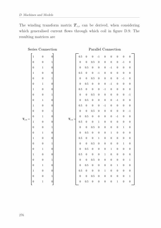
D Machines and Models
The winding transform matrix T c,e can be derived, when considering
which generalised current flows through which coil in figure D.9. The
resulting matrices are
276
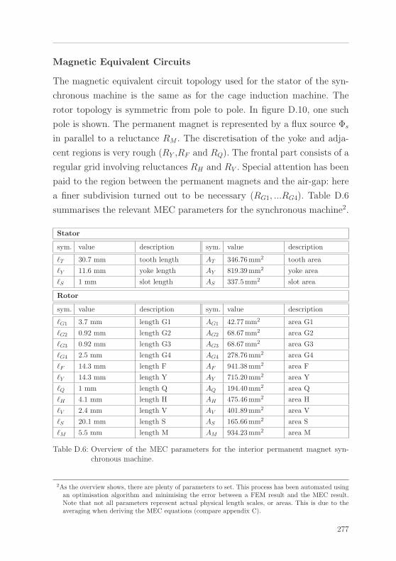
Magnetic Equivalent Circuits
The magnetic equivalent circuit topology used for the stator of the syn-
chronous machine is the same as for the cage induction machine. The
rotor topology is symmetric from pole to pole. In figure D.10, one such
pole is shown. The permanent magnet is represented by a flux source Φs
in parallel to a reluctance RM . The discretisation of the yoke and adja-
cent regions is very rough (RY ,RF and RQ). The frontal part consists of a
regular grid involving reluctances RH and RV . Special attention has been
paid to the region between the permanent magnets and the air-gap: here
a finer subdivision turned out to be necessary (RG1, ...RG4). Table D.6
summarises the relevant MEC parameters for the synchronous machine2.
Stator
sym. value description sym. value description
�T 30.7 mm tooth length AT 346.76mm2 tooth area
�Y 11.6 mm yoke length AY 819.39mm2 yoke area
�S 1 mm slot length AS 337.5mm2 slot area
Rotor
sym. value description sym. value description
�G1 3.7 mm length G1 AG1 42.77mm2 area G1
�G2 0.92 mm length G2 AG2 68.67mm2 area G2
�G3 0.92 mm length G3 AG3 68.67mm2 area G3
�G4 2.5 mm length G4 AG4 278.76mm2 area G4
�F 14.3 mm length F AF 941.38mm2 area F
�Y 14.3 mm length Y AY 715.20mm2 area Y
�Q 1 mm length Q AQ 194.40mm2 area Q
�H 4.1 mm length H AH 475.46mm2 area H
�V 2.4 mm length V AV 401.89mm2 area V
�S 20.1 mm length S AS 165.66mm2 area S
�M 5.5 mm length M AM 934.23mm2 area M
Table D.6: Overview of the MEC parameters for the interior permanent magnet syn-chronous machine.
2As the overview shows, there are plenty of parameters to set. This process has been automated usingan optimisation algorithm and minimising the error between a FEM result and the MEC result.Note that not all parameters represent actual physical length scales, or areas. This is due to theaveraging when deriving the MEC equations (compare appendix C).
277
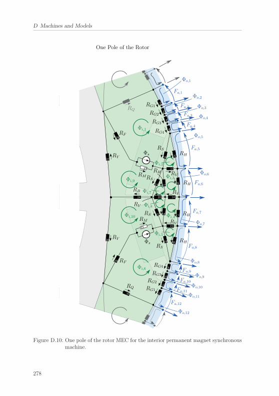
D Machines and Models
Fa,1
Fa,2
Fa,3
Fa,4
Fa,5
Fa,6
Fa,7
Fa,8
Fa,9
Fa,10
Fa,11
Fa,12
Φo,1
Φo,2
Φo,3
Φo,4
Φo,5
Φo,6
Φo,7
Φo,8
Φo,9
Φo,10
Φo,11
Φo,12
Φi,1
Φi,2
Φi,3
Φi,4
Φi,5
Φi,6
Φi,7
Φi,8
Φi,9
Φi,10
Φs
Φs
One Pole of the Rotor
RG1
RG2
RG3
RG4RF
RY
RM
RY
RF
RM
RQ
RS
RS
RS
RS
RG1
RG2
RG3
RG4
RH
RH
RH
RH
RV
RV
RV
RB
RV
RH
RQ
Figure D.10: One pole of the rotor MEC for the interior permanent magnet synchronousmachine.
278
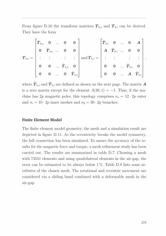
From figure D.10 the transform matrices T b,o and T b,i can be derived.
They have the form
T b,o =
⎡⎢⎢⎢⎢⎢⎢⎢⎢⎢⎢⎣
T b,o 0 ... 0 0
0 T b,o ... 0 0
......
......
0 0 ... T b,o 0
0 0 ... 0 T b,o
⎤⎥⎥⎥⎥⎥⎥⎥⎥⎥⎥⎦andT b,i =
⎡⎢⎢⎢⎢⎢⎢⎢⎢⎢⎢⎣
T b,i 0 ... 0 A
A T b,i ... 0 0
......
......
0 0 ... T b,i 0
0 0 ... A T b,i
⎤⎥⎥⎥⎥⎥⎥⎥⎥⎥⎥⎦,
where T b,o and T b,i are defined as shown on the next page. The matrix A
is a zero matrix except for the element A(30, 1) = −1. Thus, if the ma-
chine has 2p magnetic poles, this topology comprises no = 12 · 2p outer
and ni = 10 · 2p inner meshes and nb = 30 · 2p branches.
Finite Element Model
The finite element model geometry, the mesh and a simulation result are
depicted in figure D.11. As the eccentricity breaks the model symmetry,
the full crossection has been simulated. To assure the accuracy of the re-
sults for the magnetic force and torque, a mesh refinement study has been
carried out. The results are summarised in table D.7. Chossing a mesh
with 73551 elements and using quadrilateral elements in the air-gap, the
error can be estimated to be always below 1%. Table D.8 lists some at-
tributes of the chosen mesh. The rotational and eccentric movement are
considered via a sliding band combined with a deformable mesh in the
air-gap.
279
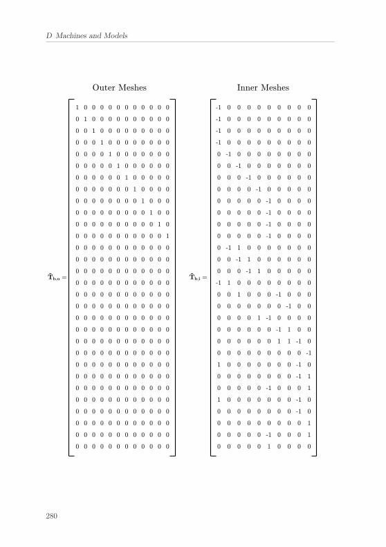
D Machines and Models
280
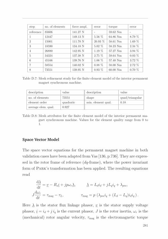
step no. of elements force ampl. error torque error
reference 85606 141.27 N - 59.62 Nm -
1 12447 149.13 N 5.56 % 64.86 Nm 8.79 %
2 15001 111.70 N 20.93 % 58.61 Nm 1.69 %
3 18590 134.18 N 5.02 % 58.23 Nm 2.34 %
4 26880 142.95 N 1.19 % 57.27 Nm 3.94 %
5 34324 137.38 N 2.75 % 59.64 Nm 0.03 %
6 45166 139.76 N 1.06 % 57.40 Nm 3.72 %
7 58554 140.02 N 0.88 % 58.00 Nm 2.72 %
8 73551 139.95 N 0.93 % 60.00 Nm 0.70 %
Table D.7: Mesh refinement study for the finite element model of the interior permanentmagnet synchronous machine.
description value description value
no. of elements 73551 shape quad/triangular
element order quadratic min. element qual. 0.18
average elem. qual. 0.927
Table D.8: Mesh attributes for the finite element model of the interior permanent ma-gnet synchronous machine. Values for the element quality range from 0 to1.
Space Vector Model
The space vector equations for the permanent magnet machine in both
validation cases have been adapted from Vas [136, p.736]. They are expres-
sed in the rotor frame of reference (dq-frame), where the power invariant
form of Park’s transformation has been applied. The resulting equations
read
dλ
dt= v −Rsi+ jpωrλ, λ = Ldid + jLqiq + λpm,
Jdωrdt
= τmag − τL, τmag = p (λpmiq + (Ld − Lq)idiq ) .
Here λ is the stator flux linkage phasor, v is the stator supply voltage
phasor, i = id+ j iq is the current phasor, J is the rotor inertia, ωr is the
(mechanical) rotor angular velocity, τmag is the electromagnetic torque
281
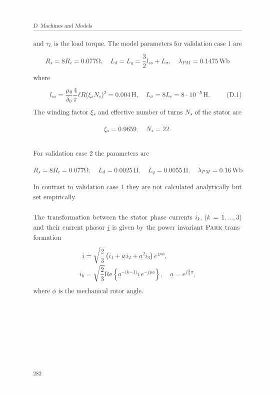
D Machines and Models
and τL is the load torque. The model parameters for validation case 1 are
Rs = 8Rc = 0.077Ω, Ld = Lq =3
2lss + Lσ, λPM = 0.1475Wb
where
lss =μ0δ0
4
π�R(ξsNs)
2 = 0.004H, Lσ = 8Lc = 8 · 10−5H. (D.1)
The winding factor ξs and effective number of turns Ns of the stator are
ξs = 0.9659, Ns = 22.
For validation case 2 the parameters are
Rs = 8Rc = 0.077Ω, Ld = 0.0025H, Lq = 0.0055H, λPM = 0.16Wb.
In contrast to validation case 1 they are not calculated analytically but
set empirically.
The transformation between the stator phase currents ik, (k = 1, ..., 3)
and their current phasor i is given by the power invariant Park trans-
formation
i =
√2
3
(i1 + a i2 + a2i3
)ejpφ,
ik =
√2
3Re{a−(k−1)i e−jpφ
}, a = ej
23π,
where φ is the mechanical rotor angle.
282
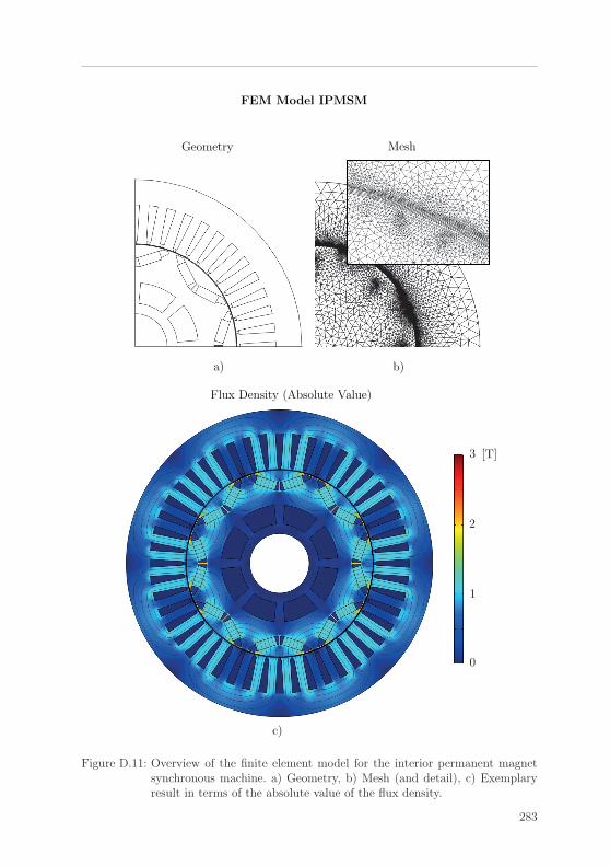
a) b)
c)
Geometry Mesh
Flux Density (Absolute Value)
[T]3
2
1
0
FEM Model IPMSM
Figure D.11: Overview of the finite element model for the interior permanent magnetsynchronous machine. a) Geometry, b) Mesh (and detail), c) Exemplaryresult in terms of the absolute value of the flux density.
283
Felix BoyIn the design of modern electrical drives a trend towards higher speeds and lighter structures can be observed. While increasing the power density this trend also implies stronger vibration issues. Among these phenomena lateral rotor oscillations due to unbalanced magnetic pull are of particular interest: strong lateral vibrations may lead to rotor-stator contact destroying the system in extreme cases.
In this work an electromechanical model is established to describe such rotordynamic vibrations. It is applicable to all kinds of rotating field machines and captures arbitrary transient states. The model describes both currents and rotor motion in a fully coupled manner. It accounts for higher harmonics in the air-gap flux density, magnetic saturation and parallel branches in the winding. The model is vali-dated by comparing it to finite element simulations, measurements and space vector models. The examples chosen are a cage induction machine and an permanent magnet synchronous machine.
Using the model self-excited rotor oscillations have been investiga-ted. Based on several simulation studies simple formulae for critical speeds concerning these vibrations have been established.
9 783737 609166
ISBN 978-3-7376-0916-6
Modelling the Rotordynamics of Saturated Electrical Machines
due to Unbalanced Magnetic Pull


