1

Geophysical investigation of landslides: A review

DENIS JONGMANS et STEPHANE GARAMBOIS

‘Laboratoire Interdisciplinaire de Recherche Impliquant la Géologie et la Mécanique’ (LIRIGM), EA 3111 UJF, Maison des Géosciences, BP 53, F-38041 Grenoble Cedex 9, France. Tel. +33 (0)476 828 046 / Fax. +33 (0)476 828 070 / E-mail : Stephane.Garambois@ujf-grenoble.fr Key words. – Landslides, Geophysical techniques, State-of-the-art Abstract. – In the last two decades, shallow geophysics has considerably evolved with the emergence of 2D spatial imaging, then 3D spatial imaging and now 4D time and space imaging. These techniques allow the study of the spatial and temporal variations of geological structures. This paper aims at presenting a current state-of-the-art on the application of surface geophysical methods to landslide characterization and focuses on recent papers (after 1990) published in peer-reviewed International Journals. Until recently, geophysical techniques have been relatively little used for the reconnaissance of landslides for at least two main reasons. The first one is that geophysical methods provide images in terms of physical parameters which are not directly linked to the geological and mechanical properties required by geologists and engineers. The second reason shown through this study probably comes from a tendency among a part of the geophysicists to overestimate the quality and reliability of the results. This paper gave the opportunity to review recent applications of the main geophysical techniques to landslide characterisation, showing both their interest and their limits. We also emphasized the geophysical image characteristics (resolution, penetration depth) which have to be provided for assessing their reliability, as well as the absolute requirements to combine geophysical methods and to calibrate them with existing geological and geotechnical data. We hope that this paper will contribute to fill the gaps between communities and to strength of using appropriate geophysical methods for landslide investigation.

Reconnaissance géophysique des glissements de terrain : Etat de l’art Mots clés. – Glissements de terrain, Investigations géophysiques, Etat de l’art Résumé. – Depuis 20 ans, la prospection géophysique à faible profondeur a considérablement évolué avec l’apparition de techniques d’imagerie 2D (x,z), puis 3D (x,y,z) et maintenant 4D (x,y,z,t), qui permettent de considérer les variations spatiales et temporelles des objets géologiques étudiés. A partir de la littérature internationale, nous tentons de faire une synthèse sur l’application des méthodes géophysiques à l’étude et au suivi des mouvements de terrain qui sont des structures complexes et évolutives. Paradoxalement, il apparaît que l’utilisation des techniques géophysiques pour la reconnaissance des mouvements de terrain est restée jusque récemment relativement limitée pour deux raisons principales. La première vient de la réticence d’une partie des ingénieurs et des géologues d’appliquer des techniques complexes qui ne fournissent pas des données géologiques, hydrogéologiques ou mécaniques directement utilisables. La seconde raison, apparue lors de cette étude, résulte de la tendance d’une partie de la communauté géophysique de surestimer la qualité et la fiabilité des résultats obtenus. A travers cette synthèse des publications, nous passons en revue les applications récentes des principales méthodes géophysiques aux mouvements de terrain en illustrant leur intérêt mais en insistant également sur leurs limites et sur les caractéristiques à fournir pour évaluer la fiabilité des images obtenues. Pour atteindre un certain degré de fiabilité, il apparaît clairement que les techniques géophysiques doivent être systématiquement combinées et calibrées par rapport aux données géologiques et géotechniques disponibles. Nous espérons que ce papier

hal-0

0196

268,

ver

sion

1 -

12 D

ec 2

007

Author manuscript, published in "Bulletin Société Géologique de France 178, 2 (2007) 101-112" DOI : 10.2113/gssgfbull.178.2.101

2

contribuera à améliorer la compréhension entre les deux communautés et à promouvoir une utilisation adaptée et combinée des techniques géophysiques modernes pour l’étude des mouvements de terrain.

hal-0

0196

268,

ver

sion

1 -

12 D

ec 2

007

3

INTRODUCTION The term landslide refers to a large variety of mass movements ranging from very slow slides in soils to rock avalanches. Several landslide classifications were proposed and the most widely used at the present time is probably the one of Cruden and Varnes [1996] which mainly considers the activity (state, distribution, style) and the description of movement (rate, water content, material type). Landslides affect all geological materials and exhibit a large variety of shapes and volumes. The characterisation of these phenomena is not a straightforward problem and may require a large volume of investigation. Reconnaissance methods, which mainly include remote-sensing and aerial techniques, geological and geomorphological mapping, geophysical and geotechnical techniques, have to be adapted to the characteristics of the landslide. According to Mc Cann and Foster [1990], a geotechnical appraisal of landslide’s stability has to consider three following issues: (1) the definition of the 3D geometry of the landslide with particular reference to failure surfaces, (2) the definition of the hydrogeological regime, (3) the detection and characterisation of the movement. Except in very peculiar cases, a landslide generally results in a modification of the morphology and of the internal structure of the affected ground mass, both in terms of hydrogeological and mechanical properties. Mapping the surface area affected by the landslide is usually done by observation of aerial photographs or remote-sensing images [Van Westen, 2004] which indicate the topographical expression of the landslide. However, if the landslide is ancient or little active, its morphologic features and boundaries may have been degraded by erosion and surface observations and measurements have to be supported by reconnaissance at depth (Dikau et al., 1996). Also, the definition of the 3D shape of the unstable body requires the investigation of the slide mass down to the undisturbed rock or soil. Conventional geotechnical techniques, which mainly include boreholes, penetration tests (when possible) and trenching [Fell et al., 2000], allow a detailed geological description and mechanical characterisation (eventually through laboratory tests) of the material, defining the vertical boundary of the slide and the parameters required for slope stability analysis. These techniques only give punctual information and their use is limited by the difficulty of drilling onto steep and unstable slopes.

Ground modifications due to a landslide are likely to generate changes of the geophysical parameters characterizing the ground, which can be used to map the landslide body and to monitor its motion. Since the pioneering work of Bogoslovsky and Ogilvy [1977], geophysical techniques have been increasingly used but relatively little referenced for landslide investigation purposes, with a growth of interest during these last few years. Among the reasons explaining the reluctance to employ geophysical techniques, one can mention the relative difficulty of deploying geophysical layouts (although the expense is far less than the one required for drilling), the limitations of most ancient geophysical methods to adequately investigate a 3D structure, and the problem of linking the measured geophysical parameters to geotechnical properties. This last aspect made probably many geotechnical engineers reluctant to use geophysical methods. In a recent review of the state-of-the-art of geotechnical engineering of natural slopes, cuts and fills in soil, Fell et al. [2000] evaluated that there are few landslide situations where geophysical techniques are a great deal of value. The recent emergence of 2D and 3D geophysical imaging techniques and the efforts of manufacturers to provide reliable and portable equipments have dramatically increased the attractiveness of geophysical techniques for landslide applications and, even if the relation between geophysical parameters and geological/geotechnical properties is still posed, these methods now appear as major tools for investigating and monitoring landslides.

This paper aims at presenting a current state-of-the-art on the application of surface geophysical methods to landslide characterization. Our work is focused on recent papers (after

hal-0

0196

268,

ver

sion

1 -

12 D

ec 2

007

4

1990) published in peer-reviewed International Journals, the authors of which are mainly scientists. In order to consider the engineering expertise in this field, we also included a limited number of Proceedings of International Conferences, written by scientists and/or engineers. This paper will contribute to improve the exchange of expertise between geophysicists, geologists, geomorphologists and geotechnical engineers. GEOPHYSICAL METHODS: AN OVERVIEW Geophysics is based on the acquisition of physical measurements from which physical parameters can be deduced. It is beyond the scope of this paper to detail the different methods used for landslide investigation and their characteristics. The principle of most of these methods can be found in general books [Reynolds, 1997; Telford et al., 1990; Sharma, 1997; Kearey et al., 2002]. A review of the geophysical methods applied at the reconnaissance stage in a landslide investigation was made by Mc Cann and Forster [1990], who illustrated with several case studies from different geological settings. Recently, Hack [2000] presented in a general way and discussed various geophysical techniques for slope stability analyses, quickly examining their merits and illustrating them.

The main characteristics of geophysical methods are pointed out in the above mentioned publications and are summarized here. On the one hand, advantages of geophysical techniques are that (1) they are flexible, relatively quick and deployable on slopes, (2) they are non- invasive and give information on the internal structure of the soil or rock mass, and (3) they allow a large volume to be investigated. On the other hand, their main drawbacks are: (1) the decreasing resolution with depth, (2) the non-uniqueness of the solution for a set of data and the resulting need for calibration and (3) the indirect information they yield (physical parameters instead of geological or geotechnical properties). It is worth noting that almost all the advantages of geophysical methods correspond to disadvantages of the geotechnical techniques and vice-versa, outlining the complementarities between the two investigation techniques. A reconnaissance campaign implying geophysical techniques has to be properly designed. The method to apply depends on its adequacy to the problem to solve and on four controlling factors, which have to be thoroughly considered before any field experiment [Mc Cann and Foster, 1990]. The first and obvious one is the existence of a geophysical contrast. The presence of a geological, hydrological or mechanical boundary (e.g., the limit of the sliding mass) does not necessarily imply a variation in terms of geophysical properties. The second issue is the characteristics of the geophysical method itself, namely the penetration depth and the resolution (ability of the method to detect a body of a given size). As mentioned above, there is usually a trade-off between resolution and penetration: the deeper-the penetration, the poorer-the resolution. These limits have to be accounted for during the design of a geophysical survey. Due to the indirect information they provide, geophysical techniques have always to be calibrated by geological or geotechnical data to obtain a reliable interpretation. Finally, the performance of geophysical techniques is strongly dependent on the signal-to-noise ratio. Landslide material can be highly disturbed and consequently lead to electrical current injection difficulties or strong seismic wave attenuation. Preliminary tests are always required before designing a survey.

After processing, geophysical methods provide the variation of a physical parameter with one, two or three spatial coordinates, corresponding to 1D, 2D and 3D information, respectively. 1D information corresponds to a profile (horizontal or vertical) while 2D and 3D information are geophysical images usually obtained through an inversion process [Sharma, 1997]. Geophysical imaging (tomography) has dramatically developed during the last twenty years and has the major advantage to give continuous information of the studied body.

hal-0

0196

268,

ver

sion

1 -

12 D

ec 2

007

5

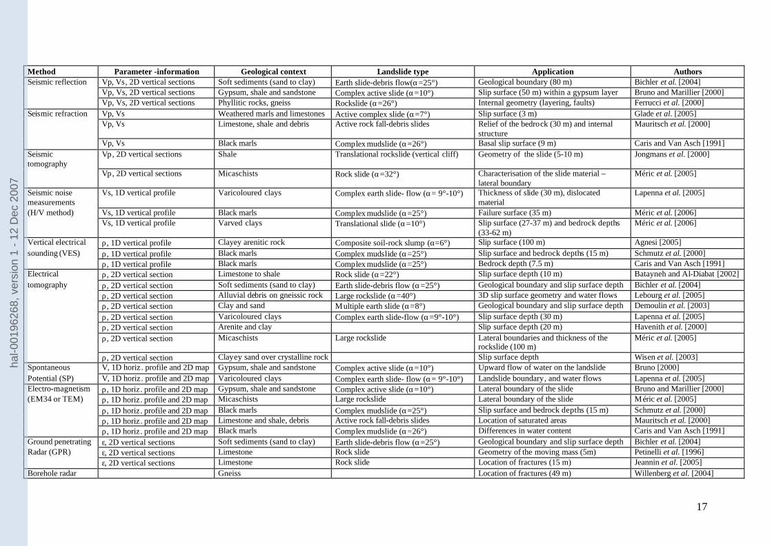
Geophysical inversion is a complex and nonlinear problem [Zhadov, 2002] and image interpretation has to be done with a critical mind, considering the already mentioned drawbacks of geophysical techniques and additional limits linked to the inversion process. It is beyond the scope of this paper to detail the geophysical imaging characteristics and only the main issues will be outlined. The obvious and necessary condition an image (model) has to fulfil is that it explains the data, i.e. the forward modelling of the derived image give results close enough to the data. This is usually assessed by a misfit error (RMS) which has to be systematically provided with the image. Even if the RMS value is low (a limit of 5% is usually considered), due to the limited measurement coverage and to errors on the data, the obtained image may only be one of the solutions explaining the data. Depending on the inversion technique, different strategies exist to address this problem of non-uniqueness: tests of inversions considering different starting models, introduction of a priori information in the inversion to constrain the solution, joint inversion of several geophysical data sets. The second issue is the image smoothness caused by most of the inversion techniques used in geophysical tomography, resulting in an inability to determine sharp layer interfaces [Wisen et al., 2003]. Also, new techniques for solving this problem are emerging, using a priori information [Wisen et al., 2005], regularization for favouring sharp boundaries in the inversion process [Zhadov, 2002] or image processing tools such as crest lines extraction process in gradient images [Nguyen et al., 2005]. Finally, most of the existing images are 2D, while a landslide is a 3D phenomenon. 2D images of 3D structures may be affected by strong artefacts which are very hard to detect [Wisen, 2005]. A judicious strategy to tackle this problem is to perform 2D and 3D forward modelling to evaluate the robustness and reliability of the obtained image. In any case, the geological or geotechnical interpretation of geophysical images has to be done by considering all the data available on the site, after a discussion between geologists, geophysicists and geotechnical engineers, and has to be clearly argued and shown. APPLICATION OF GEOPHYSICAL METHODS TO SUBSURFACE MAPPING OF LANDSLIDES Table 1 shows a synthesis of the main geophysical methods used for landslide investigation, with the measured geophysical parameter and the information type, the geological context, the landslide classification following Cruden and Varnes (1996), the geomorphology and the application (target). When available, the landslide volume is indicated. Examination of Table 1 illustrates the wide range of both geophysical techniques and geological settings in landslide applications. Geophysical prospecting was applied on various types of landslides for slope varying from a few degrees (earth slide) to vertical (rock fall). The penetration depth of the surveys ranges from 3 m to 400 m and the targets of the surveys were mainly two. By far, the major one was the location of the vertical and lateral boundaries of the slip mass or, equivalently, of the failure surface. An additional and implicit target is the mapping of the internal structure of the landslide. All geophysical methods were used with this purpose. Four main different situations can occur. In the first case, geophysical contrasts are due to the lithological changes (layering, tectonic contact or pre-slide weathering) and the failure surface mainly coincides with a geological interface or layer [Batayneh and al Diabat, 2002; Glade et al., 2005; Jongmans et al., 2000; Agnesi et al., 2005; Havenith et al., 2000; Wisen et al., 2003]. In the second case, geophysical contrasts are also controlled by lithological variations but the failure surface cuts the structure in a more complex way and may be or not deduced from the geophysical image [Bichler et al., 2004; Ferrucci et al., 2000; Mauritsch et al., 2000; Demoulin et al., 2003], depending on the landslide velocity, the heterogeneity of the material

hal-0

0196

268,

ver

sion

1 -

12 D

ec 2

007

6

and the resolution of the technique. Exceptionally (third situation), the failure surface (or potential failure) is directly detected, mainly by propagation methods [Bichler et al., 2004; Jeannin et al., 2005; Petinelli et al., 1996; Willenberg et al., 2004]. In the fourth case, the landslide develops in a globally homogeneous layer and alters its characteristics. The geophysical contrast then arises between the slide and the unaffected mass [Caris and van Asch, 1991; Méric et al., 2005; Lapenna et al., 2005; Schmutz et al., 2000; Lebourg et al., 2005; Bruno and Marillier, 2000], from the cumulative or separate action of the mecha nical dislocation, the weathering and an increase of water content. The second target of geophysical prospecting is the detection of water within the slip mass, for which electrical [Lebourg et al., 2005; Bruno and Marillier, 2000; Lapenna et al., 2005] and electromagnetic [Caris and van Asch, 1991; Mauritsch et al., 2000] methods were most applied. Critical analysis of geophysical methods in landslide investigation Seismic methods

Seismic reflection High resolution seismic reflection has been seldom used for landslide investigation [Bruno and Marillier, 2000; Bichler et al., 2004; Ferrucci et al., 2000]. Compared to other geophysical techniques, this method requires a bigger effort to deploy the geophone layouts, particularly in the conditions of rugged topography, making the technique time consuming and costly. Also, the success of shallow seismic reflection requires a good signal to noise ratio and the recording of high frequency waves to reach the desired resolution. These two conditions may be difficult to fulfil on landslides where the ground is strongly disturbed and heterogeneous, affecting the geophone-soil coupling, attenuating the seismic waves and generating scattered waves. The major interest of seismic reflection profiling is its potential for imaging the geometry of the landslide structure, such as the internal bedding or the rupture surface(s) and the robustness of processing tools compared to tomography.

All the authors carried out traditional P-wave seismic surveys, with the exception of Bichler et al. [2004], who also performed S-wave reflection profiles. The main acquisition parameters are presented in Table 2. The survey of Ferrucci et al. [2000] in a complex geological context of tectonised metamorphic rocks depicted the geological structure from 100 m to 400 m depth but failed in detecting the rupture surface, due to the too low resolution at shallow depth. Closer geophone spacing and higher fold coverage should have been adopted to reach this goal. Bruno and Marillier [2000] claimed to locate the surface of rupture for the “Boup” landslide at a depth of about 50 m (50 ms TWT) within a gypsum layer. The reflection (fig. 1) is interpreted as the contact between landslide material (disturbed gypsum) and undisturbed gypsum. A top mute was applied above 50 ms to suppress refracted waves. A shown in Figure 1, the surface rupture was at the upper detection limit of the method and the resolution can be estimated to about 5 m (a quarter of the wavelength). Bichler et al. [2004] studied the “Quesnel Forks” landslide which affected a 75 m high terrace composed of sediments deposited during the last glaciation and underlain by volcanic bedrock. The reflection surveys (both P-wave and S-wave) were made parallel to the slide motion, due to the presence of a 40° deep escarpment separating a lower block from an upper block. The method mainly succeeded in obtaining the layering boundaries within each block but had little contribution in locating the surface rupture.

Seismic refraction

hal-0

0196

268,

ver

sion

1 -

12 D

ec 2

007

7

This method is based on the interpretation of the first arrivals in the seismic signals and assumes that the velocity increases with depth [Kearey et al., 2002]. It is widely used in engineering geology for determining the depth to bedrock. For landslide investigation, the method has proved to be applicable, as both shear and compressional wave velocities are generally lower in the landslide body than in the unaffected ground. Mc Cann and Forster [1990] documented several case histories showing the use of seismic refraction for locating the undisturbed bedrock below landslides. In recent studies, the travel time data have been interpreted using delay methods [Kearey et al., 2002] like the plus-minus technique or the Generalized Reciprocal Method (GRM), which allow the mapping of an undulating refractor.

The GRM method was used by Glade et al. [2005] for positioning the failure surface of a very shallow landslide (1 to 3 m depth), which coincides with the interface between the colluvium (370 m.s-1) and marly and calcareous sediments (1100 m.s-1) of the Upper-Oligocene in the region of Rheinhessen (Germany). No signals or travel-time curves are shown to support the interpretation. Caris and Van Asch [1991] applied the plus-minus technique on a small landslide in black marl landslide (French Alps). They found a strong velocity contrast between the landslide body (350 m.s-1) and the bedrock (2800 m.s-1) which varies in depth between 4 and 9 m. Mauritsch et al. [2000] applied the GRM technique for the investigation of large landslides in the Carnic Region of southern Austria, affecting slopes with a complex geological structure made of limestone, dolomitic conglomerates, sandstones and shales. The survey pointed out a strong increase of P-wave velocity with depth (from 400 m.s-1 to 3600-4000 m.s-1) down to 30 m, with lateral velocity variations which were interpreted as lithology changes. In this context, the method was unable to identify a slip surface and mainly helped in determining the interna l composition of the sliding masses and the relief of the bedrock surface. In these case histories, the refraction method was limited to a depth between a few meters to 30 meters. This shallow penetration depth results from the method itself, which requires a relatively long profile (3 to 5 times the penetration depth as a rule of the thumb) and from the wave attenuation in the highly disturbed landslide material. In their survey, Mauritsch et al. [2000] had to switch from a sledgehammer to explosives in order to impart enough energy in the ground.

Seismic tomography The seismic tomography technique consists of inverting first-arrival times to get an image of P-wave velocity distribution in the ground. Compared to classical seismic refraction, the technique requires much more travel-time data and field effort, but allows lateral P-wave velocity variations to be determined. For landslide investigation, the technique was used in rock conditions [Méric et al., 2005; Jongmans et al., 2000] and showed a significant decrease of P-wave velocity values (division by at least a factor 2) in the slide-prone or unstable mass. Méric et al. [2005] performed a 300 m long seismic profile across the western limit of the large “Séchilienne” landslide (French Alps) affecting micaschists. Out of the unstable mass, the image (fig. 2) showed a strong vertical velocity, with Vp values ranging from 500 m.s-1 at the surface to 4000 m.s-1 at 25 m depth (sound bedrock). The same profile also pinpointed a significant lateral velocity eastward decrease (from 4000 m.s-1 to 2000 m.s-1) delineating the landslide limit. The correlation with the electrical image performed at the same place will be discussed further.

Seismic noise measurements (H/V method) Seismic noise measurements have been increasingly used during these last ten years in earthquake engineering for determining the geometry and shear wave velocity values of the

hal-0

0196

268,

ver

sion

1 -

12 D

ec 2

007

8

soil layers overlying the bedrock [Bard, 1999]. The single station method (also called the H/V technique) consists in calculating the horizontal to vertical spectral ratio of the noise records and allows the resonance frequency of the soft layer to be determined [Nakamura, 1989]. For a single homogeneous soft layer, this fundamental frequency is given by f = Vs/4h where Vs is the soft layer shear wave velocity and h is the layer thickness. Knowing an estimate of Vs allows the thickness of the soft layer to be calculated. The three main assumptions behind the method are that: 1) seismic noise is composed of surface waves; 2) the structure of the soil is 1D and; 3) the Vs contrast is large enough to generate a clear frequency peak. Difficulties also appear in heterogeneous soils (diffraction and diffusion effects) and if various frequencies can be picked (due to the presence of unexpected layers or harmonic noise, [Bonnefoy-Claudet, 2004]). As slip surfaces may generate shear wave velocity contrasts, the method can theoretically directly detect these surfaces. It was used on three landslides affecting clayey or marly terrains in the Southern Apennines [Gallipoli et al., 2000] and in the French Alps [Méric et al., this issue]. The fundamental frequency was derived from the H/V curves and used for deriving an estimate of the rupture surface depth. Depending on the studied case, these estimations were successfully compared with electrical measurements [Lapenna et al., 2003] or with geotechnical soundings or borehole measurements [Méric et al., this issue]. This easy to perform survey opens interesting perspectives for 3D investigation, with the limit of strong 2D or 3D effects which can disturb the propagation of surface waves. More complex techniques using seismic noise arrays were successfully applied by Méric et al. [this issue] to derive consistent shear-waves velocity profiles versus depth on two soil landslides.

Inversion of surface waves As slip surfaces may generate shear wave velocity contrasts due to a decrease of shear strength in the unstable zone, all methods able to show Vs variations with depth are of great interest. Beside seismic noise and SH refraction or reflection methods, the analysis of surfaces waves (SW) is now increasingly used to derive shear wave velocity versus depth in subsurface investigation [Socco and Jongmans, 2004]. The advantage of SW is that they are recorded together with P-wave refraction or reflection data, if a sufficient time length recording was considered during the acquisition. Until now, only a few 1D analyses were performed on landslides. Méric et al. [this issue] derived the dispersion curves of surface waves recorded on two landslides using the GEOPSY software developed by Wathelet et al. [2004]. In both cases, the results were consistent with other geophysical data and borehole measurements and detected quantitatively a large contrast of Vs between the sliding (250-300 m.s-1) and the stable mass (550- 800 m.s-1) at depths between 20 and 35 m. For this, the frequency range of surface waves must be large band and contain information within the stable mass, e.g. at low frequencies (the investigation depth roughly corresponds to VS/3f). Electrical methods (resistivity and spontaneous-potential)

Electrical Resistivity method The electrical resistivity method is one of the most used geophysical methods in shallow investigation [Telford et al., 1990; Reynolds, 1997]. It is based on measuring the electrical potentials between one electrode pair while transmitting a direct current between another electrode pair. The technique can be used in three ways : 1) vertical electrical sounding (VES) where electrodes are moved from a mid-point; 2) profiling where the array is moved along a direction with constant electrode spacing, and; 3) electrical tomography where a large number of electrodes and combinations of electrode pairs are used. VES is quick and easy to perform

hal-0

0196

268,

ver

sion

1 -

12 D

ec 2

007

9

and interpret. It however suffers two major drawbacks: first only vertical variations of resistivity can be considered (1D hypothesis) although measurements must be acquired over a large distance to reach large depth and second the data are likely to be explained by infinity of solutions (non-uniqueness problem). Landslides usually exhibit heterogeneous material and lateral variations of physical parameters, which make difficult the interpretation of VES. Electrical tomography, which provides a 2D (or 3D) image of electrical resistivity, has progressively taken over from the first two methods (tabl. 1) in the last decade and has emerged as a standard geophysical imaging technique known for its simplicity. However, the choice of array configuration prior to acquisition must be carefully designed, depending on the desired penetration depth, vertical and lateral resolution and ambient electrical noise. Also, as discussed before, interpretation of obtained images may be complex and should be sometimes checked using numerical modelling (e.g., anisotropy effects).

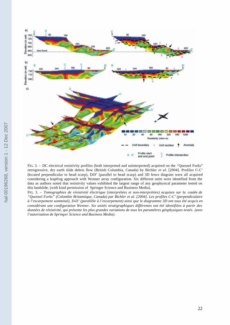
Electrical resistivity is a parameter exhibiting a large range of values [Telford et al., 1990] sensitive to various factors like the nature of material (particularly clay percentage), the water content and its conductivity, as well as the rock weathering and fracturing. This explains why this method has been the most applied for landslide investigation purposes (tabl. 1). The main target of resistivity methods prospecting for landslide investigation is the location of the rupture surface and almost all the authors having used electrical tomography claimed to have detected it in a way or another. The first case is when the surface rupture coincides with a electrically and strength contrasting geological boundary, like sha le over limestone [Batayneh and al Diabat, 2002], arenite over consolidated clay [Havenith et al., 2000] or clay over sand [Wisen et al., 2003; Demoulin et al., 2003]. Another situation is when the rupture surface is imaged by the juxtaposition of electrically contrasting units. Bichler et al. [2004] performed 4,100 m of resistivity profiles on the “Quesnel Forks” landslide. Figure 3 shows two of the electrical resistivity profiles and a 3D fence diagram of all resistivity data. Six resistivity units were identified, allowing the mapping of the rupture surface (fig. 3a).

Finally, landslides affecting homogeneous terrains can lead to a resistivity variation within the moving mass both in clayey material [Caris and van Asch, 1991; Schmutz et al., 2000; Lapenna et al., 2005] and in metamorphic rock conditions [Méric et al., 2005; Lebourg et al., 2005]. In clayey materials, the landslide body is usually associated with low resistivity values (generally between 10 and 30 Ω.m) which characterizes a high content of clay and/or water. It must be stressed out that in all the listed cases the unaffected clayey material is a compact clay or marl characterized by a resistivity over 60-75 Ω.m. The dislocation of this material by the slide allows the weathering of the minerals and the water content to be increased. Guéguen et al. [2004] were not able to detect sliding surfaces from electrical images derived on a slow clayey landslide, where slow deformation did not created observable resistivity contrast. In metamorphic rock conditions, the effect of gravitational deformation can lead to an increase [Méric et al., 2005] or decrease [Lebourg et al., 2005] of resistivity, according to the absence or presence of a water table in the involved mass. Figure 2 shows the comparison of two seismic and electrical profiles across the “Séchilienne” landslide boundary [Méric, 2005]. The electrical image shows an eastward resistivity decrease, from 200 Ω.m to 1 kΩ.m, correlated to the previously described Vp decrease. These results provide evidence the resistivity and seismic velocity variations are caused by a higher degree of fracturing in dry conditions.

Induced polarization methods were not used on landslides to our knowledge, although it has the property to distinguish clayey zones from water-saturated zones which exhibit almost same resistivities.

Spontaneous potential

hal-0

0196

268,

ver

sion

1 -

12 D

ec 2

007

10

It is well known that groundwater and associated flows contained in any landslide body play a major role in slope stability. The level of groundwater determines the supporting hydrostatic pressure, which, together with hydrodynamic pressure of seepage, are factors decreasing the landslide stability. Imaging water level and water flows within the subsurface at a large scale, as well as their fluctuations over time is a challenging problem, which resulted in specific research purposes on hydrogeophysics [Rubin and Hubbard, 2005]. Only few hydrogeophysical methods were applied on landslides, except those conducted with the Self-Potential method (SP), which is the easier to deploy and monitor.

Self-Potential surveys are conducted by measuring natural electrical potential difference between pairs of electrodes connected to a high impedance voltmeter. These natural fields represent the ground surface electric filed signature of various charging mechanisms (electrokinetic, thermoelectric, electrochemical, cultural activity) occurring at depth [Patella, 1997; Révil et al., 1999]. In absence of electrochemical processes and large telluric current, electrokinetic phenomena, describing the generation of electric fields by fluid flows, is the main source of the recorded electric field. The SP source ambiguity and the lack of quantitative interpretation on the fluid source (depth, extension) are the main limitations of the method, which was poorly used on landslides.

Bruno and Marillier [2000] measured an SP profile on the “Boup” landslide and observed that high positive SP values (40 to 120 mV) coincide with the boundary between the stable ground and the landslide material and interpret them as the electrical signature of resurgent groundwater flow. Comparable large and stable over time positive SP anomalies (up to 350 mV) were acquired by Méric et al. [2005] across the “Séchilienne” landslide. Although they noted that the shape of the SP data was highly correlated with displacement rate curve, authors did not conclude whether the source of this anomaly was electrokinecally due to a deep main water flow nearly parallel to the surface or electrochemically due to the geological structure of the movement (fractures, lead-zinc and quartz veins). However, large time-varying negative anomalies on the edge of the landslide were attributed to fluid flow variations within major faults and fractures.

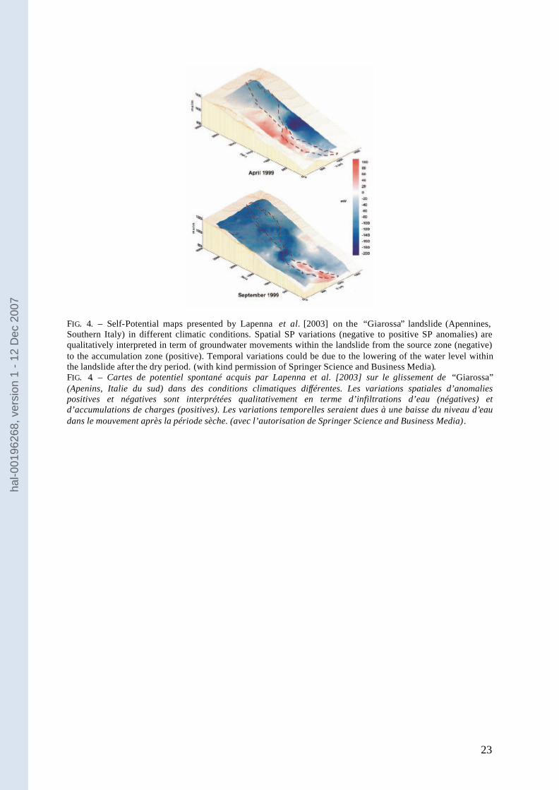
Lapenna et al. [2003] presented two SP maps carried out at different climatic conditions on the “Giarossa” landslide (fig. 5). They assume the positive and negative anomalies within the landslide are due to movements of underground water from the source zone to the accumulation zone within the landslide body. Further, SP changes over time were explained by the lowering of the water level inside the landslide body after the dry summer period. To be more quantitative, they also present SP tomographies [Patella, 1997] showing lateral boundaries of the landslide as well as geological heterogeneities. Lapenna et al. [2005] also presented an SP map of the “Varco d’Izzo” landslide that they interpreted qualitatively in term of water infiltration and charge accumulation in different zones of the landslide.

In future, increasing number of SP monitoring experiments using networks as well as improvements in numerical simulations and specific signal processing techniques [Gibert and Pessel, 2001; Sailhac and Marquis, 2001] should help the understanding of acquired data and improve hydrological information within landslides. Electromagnetic methods As shown in Table 1, electromagnetic (EM) methods were recently used by several authors for landslide investigation, mainly for determining the geometrical limits of the unstable mass. Except the work of Schmutz et al. [2000] who used TEM (Transient Electromagnetic Method) jointly with VES, EM measurements [Méric et al., 2005; Bruno and Marillier, 2000; Mauritsh et al., 2000] were usually performed in the frequency domain with two horizontal loops and a ground conductivity meter (Geonics EM 34 or EM31). The method, which yields

hal-0

0196

268,

ver

sion

1 -

12 D

ec 2

007

11

a single apparent electrical resistivity value, allows quick profiling or mapping [Reynolds, 1997]. Penetration depth depends on the coil separation (10 m, 20 m or 40 m for the EM34) and ranges from a few meters to a few tens of meters. Méric et al. [2005] and Bruno and Marillier [2000] pointed out a significant variation of apparent resistivity (between 2 and 10) at the limit between the landslide and the stable ground. In rock landslides, Bruno and Marillier [2000] and Mauritsch et al. [2000] interpreted electromagnetic data acquired with different modes and coil separations, assuming a two layer model (moving mass above stable ground). They found a relatively good agreement between the bedrock depths derived from electromagnetic interpretation and seismic results, without discussing the vertical or lateral resolution. All the authors stressed out that electromagnetic methods have to be combined with other geophysical techniques for landslide investigation. Ground Penetrating Radar (GPR) The number of published case studies using GPR data has dramatically increased during the last tens years. This success is due to: 1) its high resolution, which moreover presents a large range depending on the chosen antenna, going from a few cm to a few m; 2) its wide range of penetration depth in resistive materials; 3) its sensitivity to dielectric, electric and magnetic contrast and particularly to water content, and; 4) its light instrumentation. All of these properties make it potentially appropriate for investigations in various fields (geological, geomorphological, glaciological, environmental, geotechnical, hydrological). However, severe limitations decrease this potential for landslide investigations, as attested by the very low number of applications in this field (tabl. 1). First, GPR signals are highly attenuated in high conductive formations, thus preventing any application in soil landslides or when water saturation is higher than the target. Second, heterogeneities like fractures and blocks create diffractions decreasing dramatically the penetration depth.

Bichler et al. [2004] presented GPR reflection profiles acquired on the “Quesnel Forks” landslide using low-frequencies 50 MHz antennas, which allowed identifying seven radar facies until 25 m depth, and a possible slip surface. Barnhardt and Kayen [2000] used GPR to investigate the internal structure of two large seismically induced landslides in Anchorage (Alaska). Their surveys accurately reproduced the subsurface geometry of horst and graben structures down to a depth of 10 m and imaged finer scale features such as ground cracks and fissures. At greater depth, the presence of electrically conductive clay deposits made impossible the imaging of the failure surface. Applications of heavy field GPR investigations for rock fall stability assessment have recently emerged, favoured by the high resolution properties and penetration depth in resistive formation. Recently, Jeannin et al. [2006] performed GPR measurements with different configurations (reflection, CMP, tomography) on a limestone cliff, to evaluate their imaging potential of discontinuities inside the rock mass. GPR reflection profiles were carried out on the vertical cliff face and reached a maximum penetration of 20 m with 100 MHz antenna which gave a satisfactory resolution (approximately 25 cm) and detection power (approximately 1.5 cm). They showed that location and orientation of several reflectors coincide with the fractures observed at the surface. Roch et al. [2006] explored the potential of GPR to monitor rock walls. They acquired 3D GPR and photogrammetric data, which allowed 3D interpretation of discontinuities. Figure 5 shows the amplitude reflectivity as a function of depth with the relief of the rock fall surface. The survey pointed out a major discontinuity presenting an extent of 350 m2, which poses a problem in term of slope stability. On the contrary, the monitoring experiment did not detect any changes but yielded reproducible results under such complex conditions. All the data acquired during these two studies [Jeannin et al., 2006; Roch et al., 2006] exhibited reflectivity variations both with distance along the same fracture and with

hal-0

0196

268,

ver

sion

1 -

12 D

ec 2

007

12

frequency, which suggest that GPR measurements are sensitive to fracture properties (filling, aperture). Gravimetric studies The light instrumentation and high sensitivity to density contrasts should be an advantage of gravimetric surveys for landslide investigations, compared to other classical geophysical methods. Indeed, they allow a dense coverage and are able to detect gravimetric anomalies generated by sufficient density contrast (at least a few tenths of a g.cm-3). This condition is fulfilled when the surface failure coincides with the bedrock top or when the landslide develops generates loss of coherence and compactness in the moving mass. Del Gaudio et al. [2000] underlined that together with the support of limited other subsurface data (mechanical, geophysical, DTM), gravimetric surveys are able to provide useful information for slope stability analysis: 1) estimation of landslide body thickness and density contrasts between the moving and stable mass and, 2) location and geometry of heterogeneities within the moving mass. Blaha et al. [1998] also claimed that gravimetric surveys provided an effective contribution to the description of the structures (deformation, particular blocks, zones under tensile stress) and their dynamic control over time (by gravimetric monitoring).

However, as noted by del Gaudio et al. [2000], the use of gravimetric surveys in slope stability investigations is rather uncommon, mainly due to the long and difficult data processing and to the strong non-uniqueness of interpretation [Reynolds, 1997]. The major problem is separating anomalies of interest from the overlapping effects of other features. In the example of the “Senerchia” slump-earthflow (Southern Apennines), del Gaudio et al. [2000] performed two microgravimetric surveys in order to evaluate the potential of gravimetry to detect possible spatial-temporal density variations observed at surface. They showed that this method was able to provide information on lithological heterogeneities that may control the dynamic of landslide enlargement, if borehole measurements are available. The surveys did not show enough sensitivity to detect any temporal density changes. DISCUSSION Landslides are complex structures exhibiting a wide variety of geological, geomorphological and hydrogeological properties. Investigation of such heterogeneous structures is one of the more challenging themes for near surface geophysics. The development of 2D and 3D geophysical techniques has aroused a growing interest for assessing the landslide volume, characterising the physical properties of the landslide material and locating the groundwater flows within and around the slide. The design of a geophysical survey for landslide recognition is still a much debated question and no unique strategy came out from this review. In such heterogeneous structures, the combination of different geophysical techniques however appeared as a necessary condition for obtaining reliable results. The choice of the techniques is clearly guided by the expected contrasts in physical parameters. Other parameters, like the required penetration depth, as well as the volume and the morphology of the landslide, may also have a significant effect on the survey strategy, including for economical reasons. This review has tentatively pointed out the potentials and the limitations of geophysical methods for landslide investigation. Among these latter ones, the major difficulty of applying geophysical techniques to landslides is probably the complex relationship between the measured geophysical parameters and the desired geotechnical and hydrogeological properties, which prevents from giving a straightforward interpretation in terms of engineering properties. Outside the landslide areas, several attempts were made in

hal-0

0196

268,

ver

sion

1 -

12 D

ec 2

007

13

engineering geology to derive soil or rock properties from geophysical measurements, using experimental relationships. In soils, correlations were developed between the small-strain shear wave velocity (Vs) and penetration resistance from the CPT test [Hegazy and Mayne, 1995; Mayne and Rix, 1995; Andrus and Stokoe, 2000], mainly in geotechnical earthquake engineering. Recently, Ghose [2004] proposed a model-based integration of seismic and CPT data to derive soil parameters for sandy material. In rocks, most of the geophysical studies were aimed at characterizing the rock quality or fracturing. The application of GPR techniques for determining the fracture geometry is detailed in this paper. Apart from radar imaging, seismic methods play a more and more important role in characterizing rock sites for geotechnical purpose. As an example, a relationship between shear wave velocity and the Rock Mass Rating, which is a geotechnical factor used for tunnel design, was recently proposed by Cha et al. [2006]. In landslide investigation, similar relation ships, linking for instance geophysical parameters to the displacement rate [Méric et al., 2005] should be studied more deeply About assessing hydrogeological properties from geophysical data, outstanding results have been obtained in recent years in a new interdisciplinary field (hydrogeophysics), combining the integration of multiple sources of data and the development of comprehensive petrophysical models. The application of these methods allows hydrogeological parameters of the subsur face, like the porosity, the water content, the hydraulic conductivity to be estimated from high-resolution fluid-sensitive geophysical data (seismic, electrical, electromagnetic): a recent state-of-the art can be found in Robin and Hubbard [2005]. After this review, our feeling is that both experimental relationships and quantitative approaches should be developed in the future for landslide investigations, incorporating under-used techniques, such as spontaneous potential and induced polarization [Kemna et al., 2003] and including numerical modelling, data inversion and fusion. CONCLUSIONS Areas affected by landslides usually exhibit dramatic spatial and temporal variations of lithological and hydrogeological conditions. This review of the geophysical techniques applied to landslide reconnaissance has pointed out the large number of available methods, some of them having recently emerged. The development of 2D, and very recently 3D, geophysical imaging techniques has been a first major advance forward for investigating the complex structure of landslide areas. A second one will be the installation of permanent arrays of geophysical sensors as a part of the monitoring system of landslides. Such geophysical time- lapse surveys have recently been initiated on some landslides [Supper and Romer, 2003; Lebourg et al., 2005], mainly with a multi-electrode electrical array. Coupled with high resolution remote-sensing techniques [Van Westen, 2004] and Self-Potential monitoring systems for hydrological purposes [Méric et al., 2006], these permanent geophysical imaging systems give a new insight into the 4D deformation mechanism of a landslide. However, geophysical techniques may suffer severe drawbacks which are listed in the introduction of this paper, and they need to be combined and calibrated against geological and geotechnical data to give reliable information. Also, the complexity of landslides requires using a combination of different geophysical techniques. After this review on the application of geophysics to landslide investigation, we have the feeling that geophysicists have to make an effort in the presentation of their results. Resolution and penetration are not systematically discussed in an understandable way and the geological interpretation of the geophysical data should be more clearly and critically explained. This attitude probably partly explains the reluctance of the engineering community to use geophysical techniques, in addition to the reasons already mentioned in the introduction. It is now a challenge in the following years for

hal-0

0196

268,

ver

sion

1 -

12 D

ec 2

007

14

geophysicists to convince geologists and engineers that the 3D and 4D geophysical imaging techniques can be valuable tools for investigating and monitoring landslides. Finally, efforts should also be done towards quantitative information from geophysics in term of geotechnical parameters and hydrological properties. References AGNESI V., CAMARDAB M., CONOSCENTIA C., DI MAGGIO A., DILIBERTOC I., MADONIAC P. &

ROTIGLIANOA E. (2005). – A multidisciplinary approach to the evaluation of the mechanism that triggered the Cerda landslide (Sicily, Italy). – Geomor., 65, 101-116.

ANDRUS R.D. & STOKOE K.H. (2000). – Liquefaction resistance of soils from shear-wave velocity. – J. Geotech. Geoenv. Eng., ASCE, 126, 1015-1025.

BARD P.-Y. (1999). – Microtremor measurements: a tool for site effect estimation? – In: Proc. 2nd Int. Symp. on the Effects of Surface Geology on Seismic Motion. Yokohama, December 1-3, 1998, Irikura, Kudo, Okada & Sasatani (Eds), Balkema Rotterdam 1999, Vol. 3, 1251-1279.

BARNHARDT W. A. & KAYEN R. E. (2000) – Radar structure of earthquake-induced coastal landslides in Anchorage, Alaska. – Environ. Geosciences, 7, 38-45.

BATAYNEH A.T. & AL-DIABAT A.A. (2002) – Application of a two-dimensional electrical tomography technique for investigating landslides along the Amman-Dead Sera Highway, Jordan. – Env. Geol., 42, 399-403.

BICHLER A., BOBROWSKY P., BEST M., DOUMA M., HUNTER J., CALVERT T. & BURNS R. (2004). – Three-dimensional mapping of a landslide using a multi-geophysical approach: the Quesnel Forks landslide. – Landslides, 1 (1), 29-40.

BLÁHA P., MRLINA J. & NEŠVARA J. (1998). – Gravimetric investigation of slope deformations. – Expl. Geophys, Remote- Sens. and Env. J., 1, 21-24.

BOGOSLOVSKY V.A. & OGILVY A.A. (1977). – Geophysical methods for the investigation of landslides. – Geophysics, 42, 562-571.

BONNEFOY-CLAUDET S. (2004). – Nature du bruit de fond sismique : implications pour les études des effets de site. – Thèse de Doctorat, Univ. J. Fourier, Grenoble , France, 241 p.

BRUNO F. & MARILLIER F. (2000). – Test of high-resolution seismic reflection and other geophysical techniques on the Boup landslide in the Swiss Alps. – Surveys in Geophys., 21, 333–348.

CARIS J.P.T. & VAN ASCH TH.W.J. (1991). – Geophysical, geotechnical and hydrological investigations of a small landslide in the French Alps. – Eng. Geol., 31, 249-276.

CHA Y., KANG J. & JO C.H. (2006). – Application of linear-array microtremor surveys for rock mass classification in urban tunnel design. – Expl. Geophys., 37, 108-113.

CRUDEN D.M. & VARNES D.J. (1996). – Landslide types and processes. – In: Landslides investigation and mitigation, Transportation Research Board, Special Report 247, National Academy of Sciences. Washington DC., USA, 36-75.

DEL GAUDIO V., WASOWSKI J., PIERRI P., MASCIA U. & CALCAGNILE G. (2000). – Gravimetric study of a retrogressive landslide in Southern Italy. – Surveys in Geophys., 21, 391-399.

DEMOULIN A., PISSART A. & SCHROEDER C. (2003). – On the origin of late Quaternary palaeolandslides in the Liège (E Belgium) area. – Int. J. Earth Sci. (Geol Rundsch), 92, 795-805.

DIKAU R., BRUNDSEN D., SCHROTT L. & IBSEN M-L. (1996). – Landslide recognition: identification, movement and causes. – Wiley, Chichester, UK, 274 p.

FELL R., HUNGR O., LEROUEIL S. & RIEMER W. (2000). Keynote paper – Geotechnical engineering of the stability of natural slopes and cuts and fills in soil. – In: Proc. GeoEng2000, Int. Conf. on Geotechnical and Geol. Eng in Melbourne, Australia, Vol 1, Technomic Publishing, Lancaster, pp. 21-120, ISBN: 1-58716-067-6.

FERRUCCI F., AMELIO M., SORRISO-VALVO M. & TANSI C. (2000). – Seismic prospecting of a slope affected by deep-seated gravitational slope deformation: the Lago Sackung, Calabria, Italy. – Eng. Geol., 57, 53-64.

GALLIPOLI M., LAPENNA V., LORENZO P., MUCCIARELLI M., PERRONE A., PISCITELLI S. & SDAO F.

hal-0

0196

268,

ver

sion

1 -

12 D

ec 2

007

15

(2000). – Comparison of geological and geophysical prospecting techniques in the study of a landslide in southern Italy. – European J. Env. Eng. Geophys., 4, 117-128.

GIBERT D. & PESSEL M. (2001). – Identification of sources of potential fields with the continuous wavelet transform: Application to self-potential profiles. – Geophys. Res. Lett., 28, 1863-1866.

GHOSE R. (2004). – Model-based integration of seismic and CPT data to derive soil parameters. – In: (Ed.) Proc. 10th European Meeting of Environmental and Engineering Geophysics, Utrecht, The Netherlands, EAGE Publications , Houten, The Netherlands, paper B019, 4 p.

GLADE T., STARK P. & DIKAU R. (2005). – Determination of potential landslide shear plane depth using seismic refraction. A case study in Rheinhessen, Germany. – Bull. Eng. Geol. Environ., 64,151-158.

GUEGUEN P., GARAMBOIS S., CRAVOISIER S. & JONGMANS D. (2004). – Geotechnical, geophysical and seismological methods for surface sedimentary layers analysis. – In: Proc. 13th World Conf. Earth. Eng. Vancouver, BC Canada, IAEE Ed., Tokyo, paper no 1777.

HACK R. (2000). – Geophysics for slope stability. – Surveys in Geophys., 21, 423-448. HAVENITH H.B., JONGMANS D., ABDRAKMATOV K., TREFOIS P., DELVAUX D. & TORGOEV A. (2000).

– Geophysical investigations on seismically induced surface effects, case study of a landslide in the Suusamyr valley, Kyrgyzstan. – Surveys in Geophys., 21, 349-369.

HEGAZY Y.A. & MAYNE P.W. (1995). – Statistical correlations between Vs and CPT data for different soil types. – In: Proc.Cone Penetration Testing (CPT'95). Linköping, Sweden, Swedish Geotechnical Society, Göteborg, Vol. 2, 173-178.

JEANNIN M., GARAMBOIS S., GREGOIRE S. & JONGMANS D. (2006) – Multi-configuration GPR measurements for geometrical fracture characterization in limestone cliffs (Alps) – Geophysics, 71, 885-892.

JONGMANS D., HEMROULLE P., DEMANET D., RENARDY F. & VANBRABANT Y. (2000). – Application of 2D electrical and seismic tomography techniques for investigating landslides – European J. Env. Eng. Geophys., 5, 75-89.

KEAREY P., BROOKS M. & HILL I. (2002). – An Introduction to Geophysical Exploration. 3rd edition – Blackwell, Oxford, 262 pp.

KEMNA A., BINLEY A. & SLATER L. (2004). – Cross-borehole IP imaging for engineering and environmental applications. – Geophysics, 69, 97-105.

LAPENNA V., LORENZO P., PERRONE A., PISCITELLI S., RIZZO E. & SDAO F. (2003). – High-resolution geoelectrical tomographies in the study of the Giarrossa landslide (Potenza, Basilicata). – Bull. Eng. Geol. Env., 62, 259-68.

LAPENNA V., LORENZO P., PERRONE A., PISCITELLI S., RIZZO E. & SDAO F. (2005). – 2D electrical resistivity imaging of some complex landslides in Lucanian Apennine chain, southern Italy. – Geophysics, 70, B11-B18.

LEBOURG T., BINET S., TRIC E., JOMARD H. & EL BEDOUI S. (2005). – Geophysical survey to estimate the 3D sliding surface and the 4D evolution of the water pressure on part of a deep seated landslide. – Terra Nova, 17, 399-406.

MAURITSCH H.J., SEIBERL W., ARNDT R., ROMER A., SCHNEIDERBAUER K. & SENDLHOFER G.P. (2000). – Geophysical investigations of large landslides in the Carnic region of southern Austria . – Eng. Geol., 56, 373–388.

MAYNE P.W. & RIX G.J. (1995). – Correlations between shear wave velocity and cone tip resistance in clays. – Soils and Found., 35, 107-110.

MC CANN D.M. & FORSTER A. (1990). – Reconnaissance geophysical methods in landslide investigations. – Eng. Geol., 29, 59–78.

MERIC O., GARAMBOIS S., JONGMANS D., WATHELET M., CHATELAIN J.-L. & VENGEON J.-M. (2005). – Application of geophysical methods for the investigation of the large gravitational mass movement of Séchilienne, France. – Can. Geotech. J., 42, 1105-1115.

MÉRIC O., GARAMBOIS S. & ORENGO Y. (2006). – Large gravitational movement monitoring using a spontaneous potential network. – In: Proc. 19th Annual meeting of SAGEEP, Seattle, USA, EEGS Ed., Denver, USA, 6 p.

MÉRIC O., GARAMBOIS S., MALET J-P, CADET H., GUÉGUEN P. & JONGMANS D. (this issue). –

hal-0

0196

268,

ver

sion

1 -

12 D

ec 2

007

16

Seismic noise-based methods for soft-rock landslide characterization.– Bull. Soc. Géol. Fr. (this issue).

NAKAMURA Y. (1989). – A method for dynamic characteristics estimation of subsurface using microtremor on ground surface. – Quar. Report. Railway. Tech. Res. Institute, 30, 25-33.

NGUYEN F., GARAMBOIS S., JONGMANS D., PIRARD E. & LOCKE M. (2005). – Image processing of 2D resistivity data to locate precisely faults. – J. App. Geophys., 57, 260-277.

PATELLA D (1997). – Introduction to ground surface self-potential tomography. – Geophys. Prospect., 45, 653–681.

PETTINELLI E., BEAUBIEN S. & TOMMASI P. (1996). – GPR investigations to evaluate the geometry of rock slides and bulking in a limestone formation in northern Italy. – European J. Env. Eng. Geophys., 1, 271-286.

REVIL A., PEZARD P. & GLOVER E.W.J. (1999). – Streaming potential in porous media . 1, Theory of the zeta potential. – J. Geophys. Res., 104, 20,021-20,031.

REYNOLDS J.M. (1997). – An introduction to applied and environmental geophysics. – John Wiley & Sons, Chichester, 806 pp.

ROCH K.H., SCHWATAL, B. & BRUCKL E. (2006). – Potentials of monitoring rock fall hazards by GPR: considering as example the results of Salzburg. – Landslides, 3, 87-94.

RUBIN Y. & HUBBARD S. (Eds) (2005). – Hydrogeophysics. – Springer, The Netherlands, 530 pp. SAILHAC P. & MARQUIS G. (2001). – Analytic potentials for the forward and inverse modeling of SP

anomalies caused by subsurface fluid flow. – Geophys. Res. Lett., 28, 1851-1854. SCHMUTZ M., ALBOUY Y., GUÉRIN R., MAQUAIRE O., VASSAL J., SCHOTT J.-J. & DESCLOÎTRES M.

(2000). – Joint electrical and time domain electromagnetism (TDEM) data inversion applied to the Super Sauze earthflow (France). – Surveys in Geophys., 21, 371-390.

SHARMA P.V. (1997). – Environmental and engineering geophysics. – Cambridge Univ. Press, New York, 475 p.

SOCCO V. & JONGMANS D. (2004). – Special issue on Seismic Surface Waves. – Near Surf. Geophys., 2, 163-258.

SUPPER R. & RÖMER A. (2003). – New achievements in developing a high speed geoelectrical monitoring system for landslide monitoring. – In: Proc. 9th Meeting Env. Eng. Geophys., Prague, Czech Republic, EAGE Publications, Houten, The Netherlands EEGS Ed., O-004.

TELFORD W.M., GELDART L.P., SHERIF R.E. & KEYS D.A. (1990). – Applied Geophysics. – Cambridge Univ. Press, Cambridge,770 p.

VAN WESTEN C.J. (2004). – Geo-Information tools for landslide risk assessment: an overview of recent developments. – In: Proc. 9th International. Symp. Landslides, Rio de Janeiro, Brazil, Balkema, Rotterdam, 39-56.

WATHELET M., JONGMANS D. & OHRNBERGER M. (2004). – Surface wave inversion using a direct search algorithm and its application to ambient vibration measurements. – Near Surf. Geophys., 2, 221-231.

WILLENBERG H., EVANS K.F., EBERHARDT E., LOEW S., SPILLMANN T. & MAURER H.R. (2004). – Geological, geophysical and geotechnical investigations into the internal structure and kinematics of an unstable, complex sliding mass in crystalline rock. – In: Proc. 9th International. Symp. Landslides, Rio de Janeiro, Brazil, Balkema, Rotterdam, 489-494.

WISEN R., CHRISTIANSEN A.V., AUKEN E. & DAHLIN T. (2003). – Application of 2D laterally constrained inversion and 2D smooth inversion of CVES resistivity data in a slope stability investigation. – In: Proc. 9th Meeting Env. Eng. Geophys., Prague, Czech Republic, EAGE Publications, Houten, The Netherlands, O-002.

WISÉN R., AUKEN E. & DAHLIN T. (2005). – Combination of 1D laterally constrained inversion and 2D smooth inversion of resistivity data with a priori data from boreholes. – Near Surf. Geophys., 3, 71-79

ZHDANOV M.S. (2002). – Geophysical inverse theory and regularization problems. – Elsevier, Amsterdam - New-York – 628 pp.

hal-0

0196

268,

ver

sion

1 -

12 D

ec 2

007

17

Method Parameter -information Geological context Landslide type Application Authors Seismic reflection Vp, Vs, 2D vertical sections Soft sediments (sand to clay) Earth slide-debris flow(α=25°) Geological boundary (80 m) Bichler et al. [2004] Vp, Vs, 2D vertical sections Gypsum, shale and sandstone Complex active slide (α=10°) Slip surface (50 m) within a gypsum layer Bruno and Marillier [2000] Vp, Vs, 2D vertical sections Phyllitic rocks, gneiss Rockslide (α=26°) Internal geometry (layering, faults) Ferrucci et al. [2000] Seismic refraction Vp, Vs Weathered marls and limestones Active complex slide (α=7°) Slip surface (3 m) Glade et al. [2005] Vp, Vs Limestone, shale and debris Active rock fall-debris slides Relief of the bedrock (30 m) and internal

structure Mauritsch et al. [2000]

Vp, Vs Black marls Complex mudslide (α=26°) Basal slip surface (9 m) Caris and Van Asch [1991] Seismic tomography

Vp, 2D vertical sections Shale Translational rockslide (vertical cliff) Geometry of the slide (5-10 m) Jongmans et al. [2000]

Vp, 2D vertical sections Micaschists Rock slide (α=32°) Characterisation of the slide material – lateral boundary

Méric et al. [2005]

Seismic noise measurements

Vs, 1D vertical profile Varicoloured clays Complex earth slide- flow (α= 9°-10°) Thickness of slide (30 m), dislocated material

Lapenna et al. [2005]

(H/V method) Vs, 1D vertical profile Black marls Complex mudslide (α=25°) Failure surface (35 m) Méric et al. [2006] Vs, 1D vertical profile Varved clays Translational slide (α=10°) Slip surface (27-37 m) and bedrock depths

(33-62 m) Méric et al. [2006]

Vertical electrical ρ, 1D vertical profile Clayey arenitic rock Composite soil-rock slump (α=6°) Slip surface (100 m) Agnesi [2005] sounding (VES) ρ, 1D vertical profile Black marls Complex mudslide (α=25°) Slip surface and bedrock depths (15 m) Schmutz et al. [2000] ρ, 1D vertical profile Black marls Complex mudslide (α=25°) Bedrock depth (7.5 m) Caris and Van Asch [1991] Electrical ρ, 2D vertical section Limestone to shale Rock slide (α=22°) Slip surface depth (10 m) Batayneh and Al-Diabat [2002] tomography ρ, 2D vertical section Soft sediments (sand to clay) Earth slide-debris flow (α=25°) Geological boundary and slip surface depth Bichler et al. [2004] ρ, 2D vertical section Alluvial debris on gneissic rock Large rockslide (α=40°) 3D slip surface geometry and water flows Lebourg et al. [2005] ρ, 2D vertical section Clay and sand Multiple earth slide (α=8°) Geological boundary and slip surface depth Demoulin et al. [2003] ρ, 2D vertical section Varicoloured clays Complex earth slide-flow (α=9°-10°) Slip surface depth (30 m) Lapenna et al. [2005] ρ, 2D vertical section Arenite and clay Slip surface depth (20 m) Havenith et al. [2000] ρ, 2D vertical section Micaschists Large rockslide Lateral boundaries and thickness of the

rockslide (100 m) Méric et al. [2005]

ρ, 2D vertical section Clayey sand over crystalline rock Slip surface depth Wisen et al. [2003] Spontaneous V, 1D horiz. profile and 2D map Gypsum, shale and sandstone Complex active slide (α=10°) Upward flow of water on the landslide Bruno [2000] Potential (SP) V, 1D horiz. profile and 2D map Varicoloured clays Complex earth slide- flow (α= 9°-10°) Landslide boundary, and water flows Lapenna et al. [2005] Electro-magnetism ρ, 1D horiz. profile and 2D map Gypsum, shale and sandstone Complex active slide (α=10°) Lateral boundary of the slide Bruno and Marillier [2000] (EM34 or TEM) ρ, 1D horiz. profile and 2D map Micaschists Large rockslide Lateral boundary of the slide Méric et al. [2005] ρ, 1D horiz. profile and 2D map Black marls Complex mudslide (α=25°) Slip surface and bedrock depths (15 m) Schmutz et al. [2000] ρ, 1D horiz. profile and 2D map Limestone and shale, debris Active rock fall-debris slides Location of saturated areas Mauritsch et al. [2000] ρ, 1D horiz. profile and 2D map Black marls Complex mudslide (α=26°) Differences in water content Caris and Van Asch [1991] Ground penetrating ε, 2D vertical sections Soft sediments (sand to clay) Earth slide-debris flow (α=25°) Geological boundary and slip surface depth Bichler et al. [2004] Radar (GPR) ε, 2D vertical sections Limestone Rock slide Geometry of the moving mass (5m) Petinelli et al. [1996] ε, 2D vertical sections Limestone Rock slide Location of fractures (15 m) Jeannin et al. [2005] Borehole radar Gneiss Location of fractures (49 m) Willenberg et al. [2004]

hal-0

0196

268,

ver

sion

1 -

12 D

ec 2

007

18

Gravimetry γ, 1D horiz. profile and 2D map Flysch Hollow in bedrock near headscarp Del Gaudio et al. [2000] TABL. 1. – Synthesis of the geophysical methods used for landslide investigation. Vp and Vs: P-wave and S-wave seismic velocity; ρ: electrical resistivity; V: electrical potential; ε : electrical permittivity; γ: density; α: average slope gradient. The maximum penetration depth is indicated in brackets. TABL. 1. – Synthèse des méthodes géophysiques utilisées pour les investigations de glissements de terrain. Vp et Vs: vitesses sismiques des ondes P et S; ρ: résistivité électrique; V : potentiel électrique; ε: permittivité diélectrique; γ: densité ; α: pente moyenne. La profondeur maximale de pénétration est indiquée entre parenthèses.

hal-0

0196

268,

ver

sion

1 -

12 D

ec 2

007

19

TABL. 2. – Acquisition parameters used for seismic reflection profiles. TABL. 2. – Paramètres d’acquisition utilisés pour les profils de sismique réflexion.

Authors Channels [maximum fold]

Geophone type and spacing

Reflectors (shallow/deep)

Source type Profile length

Bruno and Marillier [2000] 24 – 48 [12 – 24]

30 Hz 3 m – 1 m

50 m–120 m

Sledge hammer Buffalo gun

110 m

Ferrucci et al. [2000] 24 [6]

- 10 m

100 m–400 m 0.1-0.2 kg of dynamite

1180 m

Bichler et al. [2004] 36 [18]

100 Hz (P-W) 8 Hz (S-W) 3 m

15 m–80 m 20 m–30 m

Sledge hammer (I beam for S-W)

130 m (P-W) 50 m (S-W)

hal-0

0196

268,

ver

sion

1 -

12 D

ec 2

007

20

FIG. 1. – Seismic reflection data obtained at the “Boup” landslide (Swiss Alps) by Bruno and Marillier [2000]. An acquisition test shotpoint section (top) shows the presence of two seismic reflections hyperbolas around 90 and 50 ms, presenting a poor signal-to-noise ratio. According to authors, they correspond to the Gypsum-Shale interface and to the sliding surface within gypsum, respectively. After classical seismic reflection processing, the bottom image shows poststack section after FK migration (constant velocity of 2000 m.s -1) together with geological interpretation. The reflection on the landslide sliding surface appears near the limit of resolution of the image (no data in the first 50 ms TWT). (with kind permission of Springer Science and Business Media). FIG. 1. – Données de sismique réflexion obtenues sur le glissement de terrain de “Boup” (Alpes Suisses) par Bruno & Marillier [2000]. Un point de tir test (haut) montre la présence de deux hyperboles de réflexion autour de 90 et 50 ms qui présentent un faible rapport signal sur bruit. Selon les auteurs, celles-ci correspondent respectivement à l’interface gypse-schiste et à la surface de glissement. Après un traitement des données classique l’image du bas montre la section sismique après sommation migrée par FK (vitesse constante de 2000 m.s-1) ainsi que l’interprétation géologique. La réflexion sur la surface de glissement apparaît proche de la limite de résolution de l’image (aucune donnée dans les 50 premières ms). (avec l’autorisation de Springer Science and Business Media).

hal-0

0196

268,

ver

sion

1 -

12 D

ec 2

007

21

FIG. 2. – Comparison between electrical (a) and seismic (b) tomography sections acquired at across the western limit of the large rocky landslide of “Séchilienne” (French Alps) affecting micaschists [Méric et al., 2005]. RMS values after inversion are 5% (a) and 2% (b). Out of the unstable mass, the image shows a strong vertical velocity, with Vp values ranging from 500 m/s at the surface to 4000 m/s at 25 m depth (sound bedrock) and a significant lateral velocity eastward decrease (from 4000 m/s to 2000 m/s) delineating the landslide limit. The electrical image (Wenner array configuration, RES2DINV inversion software) shows an eastward resis tivity increase, from 200 Ω .m to 1 kΩ .m, correlated to the previously described Vp decrease. (with kind permission of NRC Research Press). FIG. 2. – Comparaison entre tomographies (a) électrique et (b) sismiques acquises à travers la limite ouest du grand éboulement rocheux de “Séchilienne” (Alpes françaises) affectant des micaschists [Méric et al., 2005 ]. Les valeurs de RMS après inversion atteignent 5% (a) et 2% (b). Hors de la masse instable, l'image montre une vitesse verticale forte, avec Vp variant de 500 m/s vers la surface à 4000 m/s à la profondeur de 25 m (roche en place saine), ainsi qu’une diminution de vitesse latérale significative (de 4000 m.s-1 à 2000 m.s-1) vers l’est, séparant la limite d'éboulement. L'image électrique (configuration de Wenner, logiciel d'inversion RES2DINV) montre également une augmentation de la résistivité vers l’est, de 200 Ω .m à 1 kΩ .m, corrélée avec la diminution de Vp. (avec l’autorisation de NRC Research Press).

hal-0

0196

268,

ver

sion

1 -

12 D

ec 2

007

22

FIG. 3. – DC electrical resistivity profiles (both interpreted and uninterpreted) acquired on the “Quesnel Forks” retrogressive, dry earth slide debris flow (British Columbia, Canada) by Bichler et al. [2004]. Profiles C-C’ (located perpendicular to head scarp), D-D’ (parallel to head scarp) and 3D fence diagram were all acquired considering a leapfrog approach with Wenner array configuration. Six different units were identified from the data as authors noted that resistivity values exhibited the largest range of any geophysical parameter tested on this landslide. (with kind permission of Springer Science and Business Media). FIG. 3. – Tomographies de résistivité électrique (interprétées et non-interprétées) acquises sur la coulée de “Quesnel Forks” (Colombie Britannique, Canada) par Bichler et al. [2004]. Les profiles C-C’ (perpendiculaire à l’escarpement sommital), D-D’ (parallèle à l’escarpement) ainsi que le diagramme 3D ont tous été acquis en considérant une configuration Wenner. Six unités stratigraphiques différentes ont été identifiées à partir des données de résistivité, qui présente les plus grandes variations de tous les paramètres géophysiques testés. (avec l’autorisation de Springer Science and Business Media).

hal-0

0196

268,

ver

sion

1 -

12 D

ec 2

007

23

FIG. 4. – Self-Potential maps presented by Lapenna et al. [2003] on the “Giarossa” landslide (Apennines, Southern Italy) in different climatic conditions. Spatial SP variations (negative to positive SP anomalies) are qualitatively interpreted in term of groundwater movements within the landslide from the source zone (negative) to the accumulation zone (positive). Temporal variations could be due to the lowering of the water level within the landslide after the dry period. (with kind permission of Springer Science and Business Media). FIG. 4. – Cartes de potentiel spontané acquis par Lapenna et al. [2003] sur le glissement de “Giarossa” (Apenins, Italie du sud) dans des conditions climatiques différentes. Les variations spatiales d’anomalies positives et négatives sont interprétées qualitativement en terme d’infiltrations d’eau (négatives) et d’accumulations de charges (positives). Les variations temporelles seraient dues à une baisse du niveau d’eau dans le mouvement après la période sèche. (avec l’autorisation de Springer Science and Business Media).

hal-0

0196

268,

ver

sion

1 -

12 D

ec 2

007

24

FIG. 5. – Map of the amplitude reflectivity of GPR signals as a function of depth with the relief of the rock fall surface [Roch et al., 2006]. This map was obtained from a dense 3D GPR surveying composed of closely spaced parallel profiles deployed on the cliff face with 100 MHz antennas. The major discontinuity exhibited an extent of 350 m2. (with kind permission of Springer Science and Business Media). FIG. 5. – Carte de l’amplitude de la réflectivité de signaux GPR en fonction de la profondeur représentée avec le relief de la face de la falaise [Roch et al., 2006]. Cette carte a été obtenue à partir d’une investigation 3D par des antennes GPR à 100 MHz, constituée de profils parallèles peu espacés déployés le long de la face de la falaise. La discontinuité majeure a une extension de 350 m2. (avec l’autorisation de Springer Science and Business Media).

hal-0

0196

268,

ver

sion

1 -

12 D

ec 2

007