Embed Size (px)
Citation preview

GEOPHYSICAL SURVEY REPORT
103282-ENN-MMT-SUR-REP-SURVLOT1
REVISION B | FOR USE
MAY 2020
THOR OFFSHORE WIND FARM SITE INVESTIGATION
LOT 1
DANISH NORTH SEA AUGUST-DECEMBER 2019
MMT SWEDEN AB | SVEN KÄLLFELTS GATA 11 | SE-426 71 VÄSTRA FRÖLUNDA, SWEDEN
PHONE: +46 (0)31 762 03 00 | EMAIL: [email protected] | WEBSITE: MMT.SE
CLIENT: ENERGINET GEOPHYSICAL SURVEY REPORT LOT 1 | 103282-ENN-MMT-SUR-REP-SURVLOT1
PAGE | 2
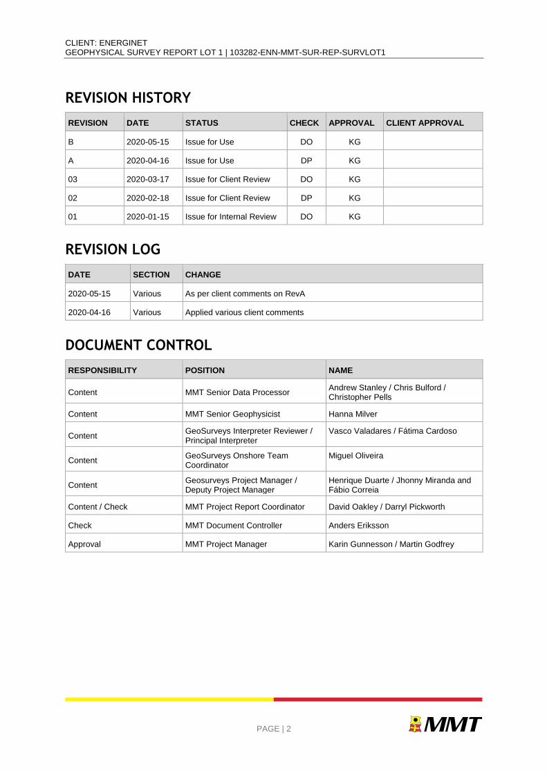
REVISION HISTORY
REVISION DATE STATUS CHECK APPROVAL CLIENT APPROVAL
B 2020-05-15 Issue for Use DO KG
A 2020-04-16 Issue for Use DP KG
03 2020-03-17 Issue for Client Review DO KG
02 2020-02-18 Issue for Client Review DP KG
01 2020-01-15 Issue for Internal Review DO KG
REVISION LOG
DATE SECTION CHANGE
2020-05-15 Various As per client comments on RevA
2020-04-16 Various Applied various client comments
DOCUMENT CONTROL
RESPONSIBILITY POSITION NAME
Content MMT Senior Data Processor Andrew Stanley / Chris Bulford / Christopher Pells
Content MMT Senior Geophysicist Hanna Milver
Content GeoSurveys Interpreter Reviewer / Principal Interpreter
Vasco Valadares / Fátima Cardoso
Content GeoSurveys Onshore Team Coordinator
Miguel Oliveira
Content Geosurveys Project Manager / Deputy Project Manager
Henrique Duarte / Jhonny Miranda and Fábio Correia
Content / Check MMT Project Report Coordinator David Oakley / Darryl Pickworth
Check MMT Document Controller Anders Eriksson
Approval MMT Project Manager Karin Gunnesson / Martin Godfrey
CLIENT: ENERGINET GEOPHYSICAL SURVEY REPORT LOT 1 | 103282-ENN-MMT-SUR-REP-SURVLOT1
PAGE | 3
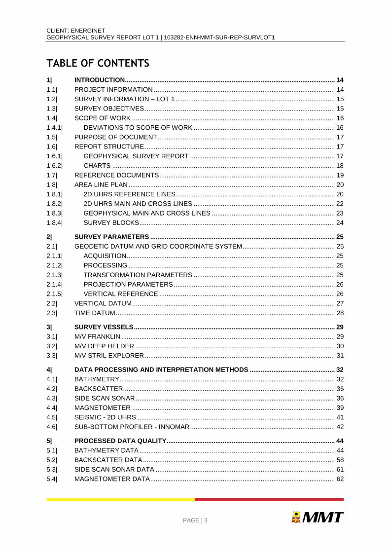
TABLE OF CONTENTS
1| INTRODUCTION .................................................................................................................... 14
1.1| PROJECT INFORMATION .................................................................................................... 14
1.2| SURVEY INFORMATION – LOT 1 ........................................................................................ 15
1.3| SURVEY OBJECTIVES ......................................................................................................... 15
1.4| SCOPE OF WORK ................................................................................................................ 16
1.4.1| DEVIATIONS TO SCOPE OF WORK .............................................................................. 16
1.5| PURPOSE OF DOCUMENT .................................................................................................. 17
1.6| REPORT STRUCTURE ......................................................................................................... 17
1.6.1| GEOPHYSICAL SURVEY REPORT ................................................................................ 17
1.6.2| CHARTS ........................................................................................................................... 18
1.7| REFERENCE DOCUMENTS ................................................................................................. 19
1.8| AREA LINE PLAN .................................................................................................................. 20
1.8.1| 2D UHRS REFERENCE LINES ........................................................................................ 20
1.8.2| 2D UHRS MAIN AND CROSS LINES .............................................................................. 22
1.8.3| GEOPHYSICAL MAIN AND CROSS LINES .................................................................... 23
1.8.4| SURVEY BLOCKS ............................................................................................................ 24
2| SURVEY PARAMETERS ...................................................................................................... 25
2.1| GEODETIC DATUM AND GRID COORDINATE SYSTEM ................................................... 25
2.1.1| ACQUISITION ................................................................................................................... 25
2.1.2| PROCESSING .................................................................................................................. 25
2.1.3| TRANSFORMATION PARAMETERS .............................................................................. 25
2.1.4| PROJECTION PARAMETERS ......................................................................................... 26
2.1.5| VERTICAL REFERENCE ................................................................................................. 26
2.2| VERTICAL DATUM ................................................................................................................ 27
2.3| TIME DATUM ......................................................................................................................... 28
3| SURVEY VESSELS ............................................................................................................... 29
3.1| M/V FRANKLIN ...................................................................................................................... 29
3.2| M/V DEEP HELDER .............................................................................................................. 30
3.3| M/V STRIL EXPLORER ......................................................................................................... 31
4| DATA PROCESSING AND INTERPRETATION METHODS ............................................... 32
4.1| BATHYMETRY ....................................................................................................................... 32
4.2| BACKSCATTER ..................................................................................................................... 36
4.3| SIDE SCAN SONAR .............................................................................................................. 36
4.4| MAGNETOMETER ................................................................................................................ 39
4.5| SEISMIC - 2D UHRS ............................................................................................................. 41
4.6| SUB-BOTTOM PROFILER - INNOMAR ................................................................................ 42
5| PROCESSED DATA QUALITY ............................................................................................. 44
5.1| BATHYMETRY DATA ............................................................................................................ 44
5.2| BACKSCATTER DATA .......................................................................................................... 58
5.3| SIDE SCAN SONAR DATA ................................................................................................... 61
5.4| MAGNETOMETER DATA ...................................................................................................... 62
CLIENT: ENERGINET GEOPHYSICAL SURVEY REPORT LOT 1 | 103282-ENN-MMT-SUR-REP-SURVLOT1
PAGE | 4
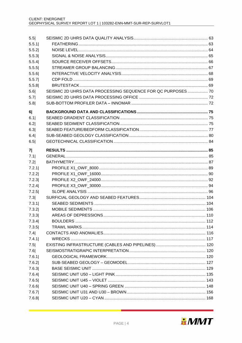
5.5| SEISMIC 2D UHRS DATA QUALITY ANALYSIS .................................................................. 63
5.5.1| FEATHERING ................................................................................................................... 63
5.5.2| NOISE LEVEL ................................................................................................................... 64
5.5.3| SIGNAL & NOISE ANALYSIS ........................................................................................... 65
5.5.4| SOURCE RECEIVER OFFSETS...................................................................................... 66
5.5.5| STREAMER GROUP BALANCING .................................................................................. 67
5.5.6| INTERACTIVE VELOCITY ANALYSIS ............................................................................. 68
5.5.7| CDP FOLD ........................................................................................................................ 69
5.5.8| BRUTESTACK .................................................................................................................. 69
5.6| SEISMIC 2D UHRS DATA PROCESSING SEQUENCE FOR QC PURPOSES .................. 70
5.7| SEISMIC 2D UHRS DATA PROCESSING OFFICE ............................................................. 72
5.8| SUB-BOTTOM PROFILER DATA – INNOMAR .................................................................... 72
6| BACKGROUND DATA AND CLASSIFICATIONS ............................................................... 75
6.1| SEABED GRADIENT CLASSIFICATION .............................................................................. 75
6.2| SEABED SEDIMENT CLASSIFICATION .............................................................................. 75
6.3| SEABED FEATURE/BEDFORM CLASSIFICATION ............................................................. 77
6.4| SUB-SEABED GEOLOGY CLASSIFICATION ...................................................................... 80
6.5| GEOTECHNICAL CLASSIFICATION .................................................................................... 84
7| RESULTS .............................................................................................................................. 85
7.1| GENERAL .............................................................................................................................. 85
7.2| BATHYMETRY ....................................................................................................................... 87
7.2.1| PROFILE X1_OWF_8000 ................................................................................................. 89
7.2.2| PROFILE X1_OWF_16000 ............................................................................................... 90
7.2.3| PROFILE X2_OWF_24000 ............................................................................................... 92
7.2.4| PROFILE X3_OWF_30000 ............................................................................................... 94
7.2.5| SLOPE ANALYSIS ........................................................................................................... 96
7.3| SURFICIAL GEOLOGY AND SEABED FEATURES ........................................................... 104
7.3.1| SEABED SEDIMENTS ................................................................................................... 104
7.3.2| MOBILE SEDIMENTS .................................................................................................... 106
7.3.3| AREAS OF DEPRESSIONS ........................................................................................... 110
7.3.4| BOULDERS .................................................................................................................... 112
7.3.5| TRAWL MARKS .............................................................................................................. 114
7.4| CONTACTS AND ANOMALIES ........................................................................................... 116
7.4.1| WRECKS ........................................................................................................................ 117
7.5| EXISTING INFRASTRUCTURE (CABLES AND PIPELINES) ............................................ 120
7.6| SEISMOSTRATIGRAPIC INTERPRETATION .................................................................... 120
7.6.1| GEOLOGICAL FRAMEWORK ........................................................................................ 120
7.6.2| SUB-SEABED GEOLOGY – GEOMODEL ..................................................................... 127
7.6.3| BASE SEISMIC UNIT ..................................................................................................... 129
7.6.4| SEISMIC UNIT U50 – LIGHT PINK ................................................................................ 135
7.6.5| SEISMIC UNIT U45 – VIOLET ....................................................................................... 143
7.6.6| SEISMIC UNIT U40 – SPRING GREEN ........................................................................ 148
7.6.7| SEISMIC UNIT U31 AND U30 – BROWN ...................................................................... 156
7.6.8| SEISMIC UNIT U20 – CYAN .......................................................................................... 168
CLIENT: ENERGINET GEOPHYSICAL SURVEY REPORT LOT 1 | 103282-ENN-MMT-SUR-REP-SURVLOT1
PAGE | 5
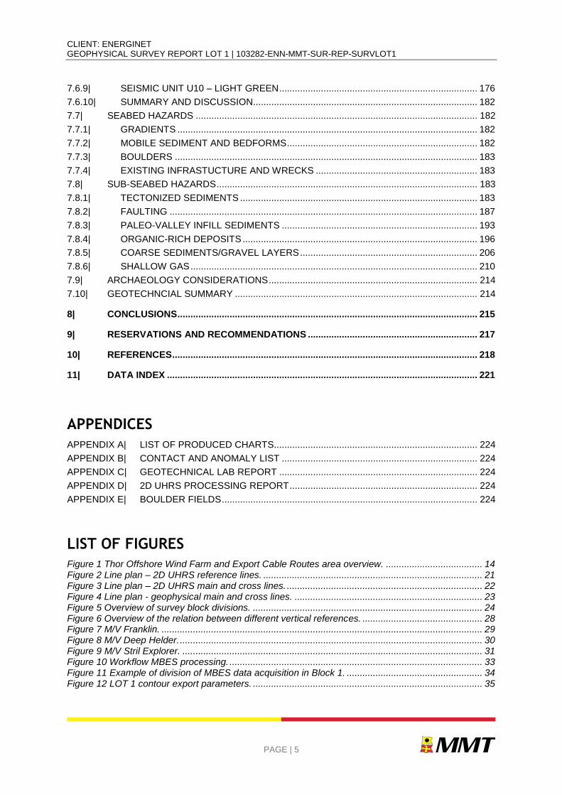
7.6.9| SEISMIC UNIT U10 – LIGHT GREEN ............................................................................ 176
7.6.10| SUMMARY AND DISCUSSION ...................................................................................... 182
7.7| SEABED HAZARDS ............................................................................................................ 182
7.7.1| GRADIENTS ................................................................................................................... 182
7.7.2| MOBILE SEDIMENT AND BEDFORMS ......................................................................... 182
7.7.3| BOULDERS .................................................................................................................... 183
7.7.4| EXISTING INFRASTUCTURE AND WRECKS .............................................................. 183
7.8| SUB-SEABED HAZARDS .................................................................................................... 183
7.8.1| TECTONIZED SEDIMENTS ........................................................................................... 183
7.8.2| FAULTING ...................................................................................................................... 187
7.8.3| PALEO-VALLEY INFILL SEDIMENTS ........................................................................... 193
7.8.4| ORGANIC-RICH DEPOSITS .......................................................................................... 196
7.8.5| COARSE SEDIMENTS/GRAVEL LAYERS .................................................................... 206
7.8.6| SHALLOW GAS .............................................................................................................. 210
7.9| ARCHAEOLOGY CONSIDERATIONS ................................................................................ 214
7.10| GEOTECHNCIAL SUMMARY ............................................................................................. 214
8| CONCLUSIONS ................................................................................................................... 215
9| RESERVATIONS AND RECOMMENDATIONS ................................................................. 217
10| REFERENCES ..................................................................................................................... 218
11| DATA INDEX ....................................................................................................................... 221
APPENDICES
APPENDIX A| LIST OF PRODUCED CHARTS .............................................................................. 224
APPENDIX B| CONTACT AND ANOMALY LIST ........................................................................... 224
APPENDIX C| GEOTECHNICAL LAB REPORT ............................................................................ 224
APPENDIX D| 2D UHRS PROCESSING REPORT ........................................................................ 224
APPENDIX E| BOULDER FIELDS .................................................................................................. 224
LIST OF FIGURES
Figure 1 Thor Offshore Wind Farm and Export Cable Routes area overview. ..................................... 14 Figure 2 Line plan – 2D UHRS reference lines. .................................................................................... 21 Figure 3 Line plan – 2D UHRS main and cross lines. ........................................................................... 22 Figure 4 Line plan - geophysical main and cross lines. ........................................................................ 23 Figure 5 Overview of survey block divisions. ........................................................................................ 24 Figure 6 Overview of the relation between different vertical references. .............................................. 28 Figure 7 M/V Franklin. ........................................................................................................................... 29 Figure 8 M/V Deep Helder. .................................................................................................................... 30 Figure 9 M/V Stril Explorer. ................................................................................................................... 31 Figure 10 Workflow MBES processing. ................................................................................................. 33 Figure 11 Example of division of MBES data acquisition in Block 1. .................................................... 34 Figure 12 LOT 1 contour export parameters. ........................................................................................ 35
CLIENT: ENERGINET GEOPHYSICAL SURVEY REPORT LOT 1 | 103282-ENN-MMT-SUR-REP-SURVLOT1
PAGE | 6
Figure 13 Example of exported contours with 50 cm interval near the south eastern corner of LOT 1.35 Figure 14 Workflow side scan sonar processing (1 of 2). ..................................................................... 38 Figure 15 Workflow side scan sonar processing (2 of 2). ..................................................................... 38 Figure 16 Data example for Deep Helder from B2. ............................................................................... 39 Figure 17 Data example for Franklin from B4. ...................................................................................... 40 Figure 18 Workflow MAG processing (1 of 2). ...................................................................................... 40 Figure 19 Workflow MAG processing (2 of 2). ...................................................................................... 41 Figure 20 Workflow SBP processing (1 of 2). ....................................................................................... 42 Figure 21 Workflow SBP processing (2 of 2). ....................................................................................... 43 Figure 22 Cross section through Block 1. ............................................................................................. 45 Figure 23 Standard deviation at 95% confidence interval for the Lot 1 survey area. ........................... 46 Figure 24 Example of MBES data acquired during good weather ........................................................ 47 Figure 25 Example of MBES data acquired during poor weather ......................................................... 48 Figure 26 QC surfaces (pink and blue cells) highlighting boulders in Block 1. ..................................... 49 Figure 27 Total Vertical Uncertainty surface for Lot 1. .......................................................................... 50 Figure 28 Cross sections through areas of high TVU values in the southwest corner or Lot 1. ........... 51 Figure 29 Total Horizontal Uncertainty surface for Lot 1. ...................................................................... 52 Figure 30 Potentially anomalous MBES contact at 423677 E, 6261046 N. .......................................... 54 Figure 31 Accepted soundings. ............................................................................................................. 55 Figure 32 Potentially anomalous MBES contact at 414316 E, 6232583 N. .......................................... 56 Figure 33 Accepted soundings. ............................................................................................................. 57 Figure 34 Overview of backscatter intensity mosaic for Lot 1. .............................................................. 59 Figure 35 Backscatter mosaic with artefacts but strong delineation of sediment boundaries. ............. 60 Figure 36 Example of good SSS data from block 1. ............................................................................. 61 Figure 37 Example SSS image from block 4. ........................................................................................ 61 Figure 38 Example SSS image from block 4 acquired onboard Franklin. ............................................ 62 Figure 39 Mag profile showing low background noise level, from Deep Helder in block 3. .................. 62 Figure 40 Mag profile showing higher background noise level, from Deep Helder in block 3. ............. 63 Figure 41 Feathering plot calculated for the line B2_OWF_2D_13200_01. ......................................... 64 Figure 42 Feathering plot calculated for the line BX3_OWF_27000. .................................................... 64 Figure 43 Noise levels recorded on Start of Line B1_OWF_2D_11760. .............................................. 65 Figure 44 Noise levels recorded on End of Line B1_OWF_2D_11760. ................................................ 65 Figure 45 Noise file shot gather showing vessel noise ......................................................................... 66 Figure 46 Shot gather for seismic profile M202..................................................................................... 66 Figure 47 Profile B2_OWF_2D_13440 in channel domain ................................................................... 67 Figure 48 200 shots from profile B2_OWF_2D_13440 in channel domain .......................................... 67 Figure 49 Streamer balancing for line B3_OWF_2D_20160. Vertical scale in TWT (ms). ................... 68 Figure 50 Velocity Analysis display for line B2_OWF_2D_15360......................................................... 68 Figure 51 Trace fold values plotted on the top of stacked sections for line B2_OWF_2D_14160........ 69 Figure 52 Brutestack for profile Sparker_Verification_EW. ................................................................... 70 Figure 53 Processing workflow applied to the seismic lines. ................................................................ 71 Figure 54 Innomar data showing achieved penetration in a channel, beneath H1. .............................. 73 Figure 55 Innomar data showing a minor data gap ............................................................................... 74 Figure 56 Innomar data showing an instance of bubble rush ............................................................... 74 Figure 57 Lot 1 survey area with the tile schema used for the description of results. .......................... 86 Figure 58 Overview of the bathymetry data. ......................................................................................... 88 Figure 59 Profiles across Lot 1 showing depth relative to DTU15 MSL. ............................................... 89 Figure 60 Broad banks of sediment in the Northwest of the survey area with sandwave bedforms. ... 90 Figure 61 MBES data with profile. ......................................................................................................... 91 Figure 62 MBES data with profile. ......................................................................................................... 92 Figure 63 MBES image depicting sandwaves and ripples in the southern central area. ...................... 93 Figure 64 MBES image with profile to show south to north seabed gradient in the southwest corner. 94 Figure 65 MBES image with profile showing features in the central south area. .................................. 95 Figure 66 Possible boulder contact with 43° slope angle...................................................................... 97 Figure 67 Accepted soundings over suspected boulder contact in Figure 66. ..................................... 98 Figure 68 Bedform feature with slope angles up to 43° located centrally within Lot 1. ......................... 99
CLIENT: ENERGINET GEOPHYSICAL SURVEY REPORT LOT 1 | 103282-ENN-MMT-SUR-REP-SURVLOT1
PAGE | 7
Figure 69 Convoluted form of step-like ridges with slope angles up to 37°. ....................................... 100 Figure 70 Slope angles over a sand wave field near the centre of the survey area. .......................... 102 Figure 71 Ripples located outside of a sandwave area with moderate slope angles. ........................ 103 Figure 72 Overview of seabed sediments. .......................................................................................... 105 Figure 73 SSS example of DIAMICTON (low to high acoustic return). ............................................... 106 Figure 74 Distribution of sand wave, megaripples and ripples in Lot 1 ............................................... 107 Figure 75 76 SSS example of featureless SAND ................................................................................ 108 Figure 77 MBES DTM image of SAND and gravelly SAND to sandy GRAVEL with ripples. ............. 108 Figure 78 Distribution of areas of mass transport deposits in Lot 1. ................................................... 109 Figure 79 Distribution of areas of depressions in relation to sub-surface gas in Lot 1. ...................... 110 Figure 80 Distribution of areas of depressions in relation to sand waves in Lot 1. ............................. 111 Figure 81 SSS example of SAND (low acoustic return) with depressions. ......................................... 112 Figure 82 Distribution of boulder fields and individual isolated boulders. ........................................... 113 Figure 83 Distribution of trawl marks in Lot 1. ..................................................................................... 114 Figure 84 SSS example of trawl marks in gravelly SAND to sandy GRAVEL with ripples. ................ 115 Figure 85 Overview of wreck locations within and in close vicinity of Lot 1. ....................................... 118 Figure 86 MBES image of wreck S_DH_B01_0199. ........................................................................... 119 Figure 87 MBES image of wreck S_DH_B03_0559. ........................................................................... 120 Figure 88 Major Danish structural elements (After Stemmerik et al., 2000); site location in red. ....... 121 Figure 89 Regional geological map (After Nielsen et al., 2008); site location in red........................... 122 Figure 90 The quaternary glaciations and an overview of Quaternary valleys in northwest Europe. . 124 Figure 91 General stratigraphy model of the geology in the eastern Danish North Sea. ................... 126 Figure 92 Seismic Profile B3_OWF_2D_22080 .................................................................................. 128 Figure 93 Map showing the lateral extent of T99 ............................................................................... 130 Figure 94 Depth below seabed of T99. ............................................................................................... 131 Figure 95 Profile B3_OWF_2D_21600 displaying the seismic character of the Base Seismic Unit. .. 132 Figure 96 Profile B3_OWF_2D_23000 displaying several erosive surfaces within the SU98. ........... 133 Figure 97 Profile BX1_OWF_7000_P2 displaying the SU99 interpreted as Miocene deposits. ......... 134 Figure 98 Map showing the lateral extent of H50. ............................................................................... 136 Figure 99 Map showing the lateral extent of H50. ............................................................................... 137 Figure 100 Thickness of unit U50. ...................................................................................................... 138 Figure 101 Profile B2_OWF_2D_17040 .............................................................................................. 139 Figure 102 Profile BX2_OWF_11000 displaying Seismic Unit U50, horizon H50 (light pink). ............ 140 Figure 103 Presence of shallow gas within seismic Unit U50, line B3_OWF_2D_20400. ................. 141 Figure 104 Profile BX2_OWF_11000 displaying very fine laminated deposits ................................... 142 Figure 105 Map showing the lateral extent of H45. ............................................................................. 143 Figure 106 Map showing the lateral extent of H45. ............................................................................. 144 Figure 107 Thickness of unit U45. ....................................................................................................... 145 Figure 108 Profile BX2_OWF_24000 displaying the laminated dipping layers ................................... 146 Figure 109 Profile B1_OWF_2D_3120 displaying sub-parallel facies ................................................ 147 Figure 110 Map showing the lateral extent of H40. ............................................................................. 149 Figure 111 Depth below seabed of H40. ............................................................................................. 150 Figure 112 Thickness of unit U40. ....................................................................................................... 151 Figure 113 Profile BX3_OWF_29000 displaying Seismic Unit U40, horizon H40 (green). ................. 152 Figure 114 Profile BX3_OWF_26000 displaying the seismic facies at base of Unit U40. ................. 153 Figure 115 Profile B4_OWF_2D_23760 displaying the irregular ........................................................ 154 Figure 116 Presence of shallow gas within Unit U40, line BX3_OWF_30000. ................................... 155 Figure 117 Map showing the lateral extent of H31. Units in metres below MSL. ................................ 156 Figure 118 Depth below seabed of H31. Units in metres below seabed. ........................................... 157 Figure 119 Thickness of unit U31. Units in metres. ............................................................................ 158 Figure 120 Profile B1_OWF_2D_6000 displaying chaotic reflections ................................................ 159 Figure 121 Profile BX3_OWF_29000 displaying some organisation and layering ............................. 160 Figure 122 Map showing the lateral extent of H30. ............................................................................ 161 Figure 123 Depth below seabed of H30. ............................................................................................. 162 Figure 124 Thickness of unit U30. ....................................................................................................... 163 Figure 125 Profile B3_OWF_2D_19680 displaying Seismic Unit U30, horizon H30 (brown). ............ 164
CLIENT: ENERGINET GEOPHYSICAL SURVEY REPORT LOT 1 | 103282-ENN-MMT-SUR-REP-SURVLOT1
PAGE | 8
Figure 126 Profile BX2_OWF_23000 shows the transparent reflections ............................................ 165 Figure 127 Profile B3_OWF_2D_2110 displaying oblique configurations within U30. ....................... 166 Figure 128 Presence of shallow gas within U30, line B3_OWF_2D_20400. ...................................... 167 Figure 129 Map showing the lateral extent of H20. ............................................................................ 168 Figure 130 Depth below seabed of H20. ............................................................................................. 169 Figure 131 Thickness of unit U20. ....................................................................................................... 170 Figure 132 Profile B4_OWF_2D_23520 displaying transparent facies ............................................... 171 Figure 133 Profile BX3_OWF_29000 displaying sub-parallel layering within Unit U20. ..................... 172 Figure 134 Profile BX3_OWF_27000 displaying acoustic (semi)transparency .................................. 173 Figure 135 Profile BX1_OWF_12000 shows transparent and chaotic reflections of Unit U20. .......... 174 Figure 136 Presence of shallow gas within U20 line B1_OWF_2D_4080. ......................................... 175 Figure 137 Map showing the lateral extent of H10. ............................................................................. 176 Figure 138 Depth below seabed of H10. ............................................................................................. 177 Figure 139 Thickness of H10. Units in metres. ................................................................................... 178 Figure 140 Profile BX2_OWF_22000 displaying Seismic Unit U10, horizon H10 (light green). ......... 179 Figure 141 Profile B4_OWF_2D_24480 displaying some faint internal layering ................................ 180 Figure 142 Profile BX1_OWF_15000 (a) and B4_OWF_2D_23040 (b) ............................................. 181 Figure 143 Seismic profile B3_OWF_2D_22080 displaying deformed sediments inside the SU98. .. 184 Figure 144 Seismic profile BX3_OWF_26000 displaying deformed sediments inside the SU98. ...... 185 Figure 145 Seismic profile B4_OWF_2D_24240 displaying complex deformation ............................ 186 Figure 146 Individual faults mapped across the site. .......................................................................... 188 Figure 147 Seismic profile BX3_OWF_27000 displaying faulting ....................................................... 189 Figure 148 Seismic profile B2_OWF_2D_15360 displaying faulting within unit U50. ......................... 190 Figure 149 Seismic profile B4_OWF_2D_24720 displaying faulting .................................................. 191 Figure 150 Seismic profile B3_OWF_2D_19440 displaying faulting within unit SU99. ...................... 192 Figure 151 Profile BX3_OWF_27000 displaying the channel features in different seismic units. ...... 194 Figure 152 Profile B2_OWF_2D_12960 displaying paleo-valleys within SU98. ................................. 195 Figure 153 Map showing the lateral extent of the negative impedance contrasts .............................. 196 Figure 154 Depth below seabed of HZ_sm_U20. ............................................................................... 197 Figure 155 Map showing the extent of the negative impedance contrasts ......................................... 198 Figure 156 Depth below seabed of HZ_sm_U30U31. ........................................................................ 199 Figure 157 Map showing the extent of the negative impedance contrast ........................................... 200 Figure 158 Depth below seabed of HZ_sm_U45. ............................................................................... 201 Figure 159 Profile B2_OWF_2D_13200 displaying negative impedance contrasts ........................... 202 Figure 160 – Profile B3_OWF_2D_19200 displaying negative impedance contrast .......................... 203 Figure 161 Profile B2_OWF_2D_10320 displaying negative impedance contrast ............................. 204 Figure 162 Profile BX3_OWF_3200 displaying negative impedance contrast ................................... 205 Figure 163 Map showing the lateral extent of HZ_01. ........................................................................ 206 Figure 164 Depth below seabed of HZ_01.......................................................................................... 207 Figure 165 Profile BX3_OWF_32000 displaying a possible coarse layer within U45 ......................... 208 Figure 166 – Profile BX3_OWF_2000 displaying a possible coarse layer within SU99 ..................... 209 Figure 167 Map showing the lateral extent of shallow gas. ................................................................ 210 Figure 168 Depth below seabed of HZ_gas. ....................................................................................... 211 Figure 169 Presence of shallow gas within U30, line B3_OWF_2D_20880. ...................................... 212 Figure 170 Profile B3_OWF_2D_2040 (a) and B3_OWF_2D_20880 (b) ........................................... 213
LIST OF TABLES
Table 1 Project details. .......................................................................................................................... 15 Table 2 Deviations from the Lot 1 SOW during geophysical survey, MV Franklin. ............................... 16 Table 3 Deviations from the Lot 1 SOW during survey, M/V Deep Helder. .......................................... 16 Table 4 Reference documents. ............................................................................................................. 19 Table 5 Survey line parameters. ........................................................................................................... 20 Table 6 Survey line breakdown. ............................................................................................................ 20 Table 7 Geodetic parameters used during acquisition. ......................................................................... 25 Table 8 Geodetic parameters used during processing. ........................................................................ 25

CLIENT: ENERGINET GEOPHYSICAL SURVEY REPORT LOT 1 | 103282-ENN-MMT-SUR-REP-SURVLOT1
PAGE | 9
Table 9 Transformation parameters. ..................................................................................................... 25 Table 10 Official test coordinates .......................................................................................................... 26 Table 11 Projection parameters. ........................................................................................................... 26 Table 12 Vertical reference. .................................................................................................................. 26 Table 13 Height comparison between DTU15 and DVR90. .................................................................. 27 Table 14 M/V Franklin equipment. ........................................................................................................ 29 Table 15 M/V Deep Helder equipment. ................................................................................................. 30 Table 16 M/V Stril Explorer equipment. ................................................................................................. 31 Table 17 Gridding parameters. .............................................................................................................. 41 Table 18 Seabed gradient classification. ............................................................................................... 75 Table 19 Sediment classification. .......................................................................................................... 76 Table 20 Seabed features classification. ............................................................................................... 77 Table 21 Summary of the seismic units. ............................................................................................... 81 Table 22 Summary of SSS contacts. .................................................................................................. 116 Table 23 Summary of MBES contacts ................................................................................................ 116 Table 24 Summary of magnetic anomalies. ........................................................................................ 116 Table 25 Summary of wrecks (in vicinity of and inside Lot 1), database information. ........................ 117 Table 26 Deliverables. ......................................................................................................................... 221

CLIENT: ENERGINET GEOPHYSICAL SURVEY REPORT LOT 1 | 103282-ENN-MMT-SUR-REP-SURVLOT1
PAGE | 10
ABBREVIATIONS AND DEFINITIONS BSB Below Seabed
CM Central Meridian
DTU15 Denmark Technical University 2015
DPR Daily Progress Report
DTM Digital Terrain Model
EEZ Exclusive Economic Zone
EPSG European Petroleum Survey Group
ESRI Environmental Systems Research Institute, Inc.
ETRS European Terrestrial Reference System
FME Feature Manipulation Engine
FMGT Fledermaus GeoCoder Toolbox
GIS Geographic Information System
GNSS Global Navigation Satellite System
GRS80 Geodetic Reference System 1980
GS Grab Sample
HF High Frequency
HiPAP High Precision Acoustic Positioning
HPMV High Power Marine Vibrocorer
INS Inertial Navigation System
IHO International Hydrographic Organisation
IMU Inertial Measurement Unit
ITRF International Terrestrial Reference Frame
LAT Lowest Astronomical Tide
LF Low Frequency
LGM Last Glacial Maximum
Lot 1 Investigation Area
MAG Magnetometer
MBBS Multibeam Backscatter
MBES Multibeam Echo Sounder
MIG Migrated
MMO Man Made Object
MSL Mean Sea Level
MUL Multiple Attenuated Stack
M/V Motor Vessel
OWF Offshore Wind Farm
POS MV Position and Orientation System for Marine Vessels
POSPac Position and Orientation System Package
PPS Pulse Per Second
QC Quality Control
ROTV Remotely Operated Towed Vehicle
S-CAN Scalgo Combinatorial Anti Noise
SBET Smoothed Best Estimated Trajectory
SBP Sub-Bottom Profiler
SOW Scope of Work

CLIENT: ENERGINET GEOPHYSICAL SURVEY REPORT LOT 1 | 103282-ENN-MMT-SUR-REP-SURVLOT1
PAGE | 11
SSS Side Scan Sonar
THU Total Horizontal Uncertainty
TPU Total Propagated Uncertainty
TVU Total Vertical Uncertainty
TWT Two Way Time
UHRS Ultra High Resolution Seismic
USBL Ultra Short Baseline
UTC Coordinated Universal Time
UTM Universal Transverse Mercator
UXO Unexploded Ordnance
VC Vibrocorer
CLIENT: ENERGINET GEOPHYSICAL SURVEY REPORT LOT 1 | 103282-ENN-MMT-SUR-REP-SURVLOT1
PAGE | 12
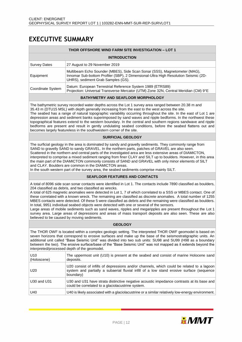
EXECUTIVE SUMMARY
THOR OFFSHORE WIND FARM SITE INVESTIGATION – LOT 1
INTRODUCTION
Survey Dates 27 August to 29 November 2019
Equipment Multibeam Echo Sounder (MBES), Side Scan Sonar (SSS), Magnetometer (MAG), Innomar Sub-bottom Profiler (SBP), 2 Dimensional-Ultra High Resolution Seismic (2D-UHRS), sediment Grab Samples (GS).
Coordinate System Datum: European Terrestrial Reference System 1989 (ETRS89) Projection: Universal Transverse Mercator (UTM) Zone 32N, Central Meridian (CM) 9°E
BATHYMETRY AND SEAFLOOR MORPHOLOGY
The bathymetric survey recorded water depths across the Lot 1 survey area ranged between 20.38 m and 35.43 m (DTU15 MSL) with depth generally increasing from the east to the west across the site. The seabed has a range of natural topographic variability occurring throughout the site. In the east of Lot 1 are depression areas and sediment banks superimposed by sand waves and ripple bedforms. In the northwest these topographical features extend to the western boundary. In the central and southern regions sandwave and ripple bedforms are present and result in gently undulating seabed conditions, before the seabed flattens out and becomes largely featureless in the southwestern corner of the site.
SURFICIAL GEOLOGY
The surficial geology in the area is dominated by sandy and gravelly sediments. They commonly range from SAND to gravelly SAND to sandy GRAVEL. In the northern parts, patches of GRAVEL are also seen. Scattered in the northern and central parts of the investigated area are less extensive areas of DIAMICTON, interpreted to comprise a mixed sediment ranging from finer CLAY and SILT up to boulders. However, in this area the main part of the DIAMICTON commonly consists of SAND and GRAVEL with only minor elements of SILT and CLAY. Boulders are common in the DIAMICTON areas. In the south western part of the survey area, the seabed sediments comprise mainly SILT.
SEAFLOOR FEATURES AND CONTACTS
A total of 8096 side scan sonar contacts were identified in Lot 1. The contacts include 7890 classified as boulders, 204 classified as debris, and two classified as wrecks. A total of 625 magnetic anomalies were detected in Lot 1, 7 of which correlated to a SSS or MBES contact. One of these correlated with a known wreck. The remaining are classified as discrete anomalies. A total number of 1255 MBES contacts were detected. Of these 5 were classified as debris and the remaining were classified as boulders. In total, 9951 individual seabed objects were detected with one or several of the sensors. Large areas of mobile sediments such as sand waves, ripples and megaripples are present throughout the Lot 1 survey area. Large areas of depressions and areas of mass transport deposits are also seen. These are also believed to be caused by moving sediments.
GEOLOGY
The THOR OWF is located within a complex geologic setting. The interpreted THOR OWF geomodel is based on seven horizons that correspond to erosive surfaces and make up the base of the seismostratigraphic units. An additional unit called “Base Seismic Unit” was divided into two sub units: SU98 and SU99 (H98 as a boundary between the two). The erosive surface/base of the “Base Seismic Unit” was not mapped as it extends beyond the interpreted/processed depth of the geomodel.
U10 (Holoscene)
The uppermost unit (U10) is present at the seabed and consist of marine Holocene sand deposits.
U20 U20 consist of infills of depressions and/or channels, which could be related to a lagoon system and partially a subaerial fluvial infill of a low stand erosive surface (sequence boundary)
U30 and U31
U30 and U31 have strata distinctive negative acoustic impedance contrasts at its base and could be correlated to a glaciolacustrine system.
U40 U40 is likely associated with a glaciolacustrine or a similar relatively low-energy environment.
CLIENT: ENERGINET GEOPHYSICAL SURVEY REPORT LOT 1 | 103282-ENN-MMT-SUR-REP-SURVLOT1
PAGE | 13
THOR OFFSHORE WIND FARM SITE INVESTIGATION – LOT 1
U45 U45 could be related to a fluviodeltaic system in a moderate energy environment.
U50
U50 consists of fine layered sediments of glaciolacustrine origin and distinct laminated facies on the seismic profiles.
Base Seismic Unit The lowermost base unit, subdivided into SU98 and SU99, is a complex seismic unit comprising deformed sediments, which could be caused by glacial tectonics, valley infills and undeformed subparallel deltaic deposits (Miocene).
SEABED AND SUB-SEABED HAZARDS
Seabed gradients
Slope angles across the site are typically very gentle (<1°) and gentle (1° to 5°). Despite the fact that sand wave areas constitute approximately 78% of the site the seafloor topography is typically gently undulating. Areas of moderate to very steep slopes are largely restricted to the edges of sand bodies and the lee slopes of the most defined sand waves. Very steep slope angles (15° to a maximum of 43°) are associated with boulders, the edges of depressions and step-like features possibly associated with slumping of sediments and succeeding sediment movement. Slope angles up to 75° were observed, but were associated with boulder-like features identified within Deep Helder data that could not be disproved as system noise.
Mobile seabed sediments
Mobile sediments are present throughout most of the surveyed area. They are most prominent in the central and northern parts. The mobile sediments comprise sand waves as well as megaripples and ripples. Areas of depressions and mass transport deposits found in conjunction to the sand waves are also believed to be caused by moving sediments.
Wreck Two wrecks were detected during the survey correlating with the background information. Wreck S_DH_B01_0199 (400110c_134) was found at 411116 m E, 6242717 m N and wreck S_DH_B03_0559, M_103 (400110c-132) was found at 421836 m E, 6242042 m N.
Cable According to available background data, there are no known cables in the area. No cables were observed in the survey area.
Pipeline According to available background data, there are no known pipelines in the area. No pipelines were observed in the survey area.
Coarse Sediments/Gravel Layers
Coarser material, such as boulders, cobbles, gravel lags and ancient wood (logs) are present in glacial environments and associated seismic records, their presence should be considered a general hazard. Coarse layers are visible within subunit SU99. The presence of sub-seabed boulders and coarse sediment/gravel layers usually constitutes a constraint on drilling and other operations as they can cause damage to equipment, affect equipment installation and ultimately cause foundation failure.
Tectonized sediments
Areas of tectonization/deformation have been observed predominately within SU98. The origin of these deformed deposits is interpreted to be glacial tectonics. Deformed deposits have geotechnical significance given their complex stress/load histories.
Paleo-valley infill sediments
Buried channels occur throughout THOR OWF site. The more relevant erosive events that carved these channels correspond to the unit base of U50. A potential geo-hazard related with the channels is the sharp contrasts in physical properties between the channel infill and surrounding units. An older system of channels (tunnel valleys) were also found within the sub unit SU98.
Organic-rich deposits
High-amplitude, negative impedance features occur within seismic units U20, U30, U31 and U45. These features are interpreted to be fine sediments, most likely organic-rich muds due to their strong negative acoustic impedance.
Shallow Gas Evidence shallow gas accumulations were found in THOR OWF site. Shallow gas accumulations occur mainly within seismic units U20, U30 and U50.
Faulting Faults are present in some units and do not greatly affect sediments younger than U30. Faults were identified within units U40 and U50. Subunits SU98 and SU99 also display several features affecting and displacing the sediments.
CLIENT: ENERGINET GEOPHYSICAL SURVEY REPORT LOT 1 | 103282-ENN-MMT-SUR-REP-SURVLOT1
PAGE | 14
1| INTRODUCTION
1.1| PROJECT INFORMATION
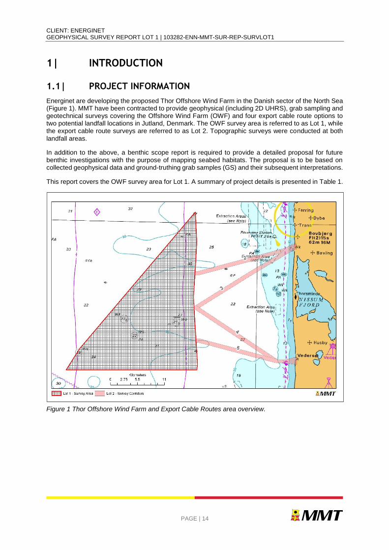
Energinet are developing the proposed Thor Offshore Wind Farm in the Danish sector of the North Sea (Figure 1). MMT have been contracted to provide geophysical (including 2D UHRS), grab sampling and geotechnical surveys covering the Offshore Wind Farm (OWF) and four export cable route options to two potential landfall locations in Jutland, Denmark. The OWF survey area is referred to as Lot 1, while the export cable route surveys are referred to as Lot 2. Topographic surveys were conducted at both landfall areas.
In addition to the above, a benthic scope report is required to provide a detailed proposal for future benthic investigations with the purpose of mapping seabed habitats. The proposal is to be based on collected geophysical data and ground-truthing grab samples (GS) and their subsequent interpretations.
This report covers the OWF survey area for Lot 1. A summary of project details is presented in Table 1.
Figure 1 Thor Offshore Wind Farm and Export Cable Routes area overview.

CLIENT: ENERGINET GEOPHYSICAL SURVEY REPORT LOT 1 | 103282-ENN-MMT-SUR-REP-SURVLOT1
PAGE | 15
Table 1 Project details.
CLIENT: Energinet
PROJECT: Thor Offshore Wind Farm Investigations Lot 1 & Lot 2
MMT SWEDEN AB (MMT) PROJECT NUMBER: 103282
SURVEY TYPE: Geophysical and Geotechnical offshore windfarm site survey
AREA: Danish North Sea
SURVEY PERIOD: August – December 2019
SURVEY VESSELS: M/V Franklin, M/V Deep Helder, M/V Stril Explorer, M/V Ping, UAS SenseFly eBee
MMT PROJECT MANAGER: Karin Gunnesson / Martin Godfrey
CLIENT PROJECT MANAGER: Jens Colberg-Larsen
1.2| SURVEY INFORMATION – LOT 1
The Lot 1 work scope comprises several tasks including:
Project Management and Administration
Geophysical surveys
2D UHRS Survey
Geotechnical survey
The Thor Offshore Wind Farm site investigation covers an approximately 440 km2 area acquired by MMT and is located roughly 20 km offshore the coast of Jutland (Figure 1).
This report covers the Lot 1 offshore wind farm survey works acquired by MMT with integrated geotechnical survey (Appendix C|) results. This report also integrates the 2D UHRS survey dataset acquired by GeoSurveys Ltd (Appendix D|)
1.3| SURVEY OBJECTIVES
The survey objectives for this project were to acquire bathymetric soundings, magnetometer, seabed imagery and sub-seabed geological information within the proposed Thor OWF site. The acquisition of these data were to provide comprehensive bathymetric soundings, seabed features maps including contact listings and shallow geological information to inform a ground model and mapping of magnetic anomalies. The interpretation of the datasets was charted and reported to inform cable route micro-routeing and subsequent engineering.
The main objectives with the surveys were:
Acquire and interpret high quality seabed and sub-seabed data for project planning and execution. As a minimum, this includes local bathymetry, seabed sediment distribution, seabed features, seabed obstructions, wrecks and archaeological sites, crossing cables and pipelines and evaluation of possible mobile sediments
Sub-bottom profiling and 2D UHRS survey along the survey lines to map shallow geological units.
Mapping of magnetic targets and to identify infrastructure crossings and large metallic debris.
Seabed sampling and testing to provide in-situ geological data to support the interpretation of the shallow geophysical survey data. In addition, several vibrocore samples were also carried
CLIENT: ENERGINET GEOPHYSICAL SURVEY REPORT LOT 1 | 103282-ENN-MMT-SUR-REP-SURVLOT1
PAGE | 16
out to provide material for subsequent analysis, as part of an Energinet funded marine archaeological study being carried out by Moesgaard Museum, Aarhus Denmark.
Ground truthing GS acquisition where necessary to inform potential environmentally sensitive habitats.
1.4| SCOPE OF WORK
For Lot 1 the following work packages are included in the scope of work (SOW):
Work Package A – Geophysical survey A geophysical survey with full coverage of the area of investigation. The survey will map the bathymetry, the static and dynamic elements of the seabed surface and the sub-surface geological soil layers.
Work Package C – Geotechnical investigations Upon completion and interpretation of the Work Package A, a geotechnical campaign to provide the soil parameters of the interpreted soil strata.
Work Package D – Reporting and data delivery The results of the investigations shall be processed, interpreted and supplied as a number of reports, charts and a set of digital deliverables.
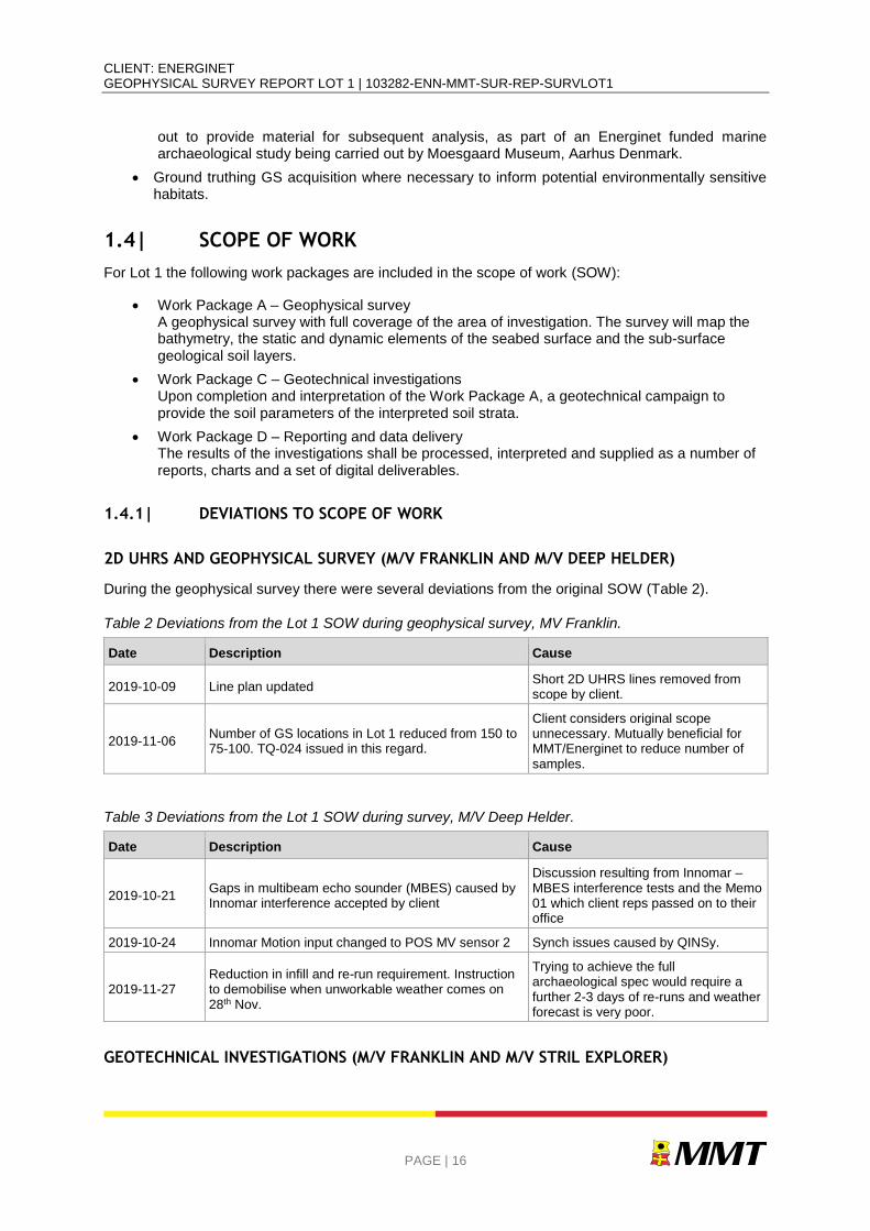
1.4.1| DEVIATIONS TO SCOPE OF WORK
2D UHRS AND GEOPHYSICAL SURVEY (M/V FRANKLIN AND M/V DEEP HELDER)
During the geophysical survey there were several deviations from the original SOW (Table 2).
Table 2 Deviations from the Lot 1 SOW during geophysical survey, MV Franklin.
Date Description Cause
2019-10-09 Line plan updated Short 2D UHRS lines removed from scope by client.
2019-11-06 Number of GS locations in Lot 1 reduced from 150 to 75-100. TQ-024 issued in this regard.
Client considers original scope unnecessary. Mutually beneficial for MMT/Energinet to reduce number of samples.
Table 3 Deviations from the Lot 1 SOW during survey, M/V Deep Helder.
Date Description Cause
2019-10-21 Gaps in multibeam echo sounder (MBES) caused by Innomar interference accepted by client
Discussion resulting from Innomar – MBES interference tests and the Memo 01 which client reps passed on to their office
2019-10-24 Innomar Motion input changed to POS MV sensor 2 Synch issues caused by QINSy.
2019-11-27 Reduction in infill and re-run requirement. Instruction to demobilise when unworkable weather comes on 28th Nov.
Trying to achieve the full archaeological spec would require a further 2-3 days of re-runs and weather forecast is very poor.
GEOTECHNICAL INVESTIGATIONS (M/V FRANKLIN AND M/V STRIL EXPLORER)
CLIENT: ENERGINET GEOPHYSICAL SURVEY REPORT LOT 1 | 103282-ENN-MMT-SUR-REP-SURVLOT1
PAGE | 17
During the geotechnical investigations for Lot 1 there were no deviations from the original SOW.
1.5| PURPOSE OF DOCUMENT
This report details the interpretation of the geophysical and geotechnical results from the Thor OWF Site Investigations.
The report summarises the conditions within the Lot 1 survey area with regards to; bathymetry, surficial geology and seabed features, contacts and anomalies, existing infrastructure, and subsurface geology. Geo-hazard identification and interpretation has also been considered.
All data obtained from the geophysical and geotechnical surveys have been correlated with each other and compared against the existing background information, in order to ground truth the survey results.
Separate reports include the Export Cable Routes surveys, Geotechnical survey results, Environmental survey and Operations reports. A full list of reports is given in Table 4 (Reference Documents).
1.6| REPORT STRUCTURE
The results from the Lot 1 survey campaign are presented in two separate reports.
Geophysical Survey Report (this report) – Includes a chart series of results. A full chart list is provided within Appendix A|.
Operations Report – Covering the field operations conducted
The Geophysical Survey Report (this report) chart series includes:
Overview Chart
Trackline Charts
Bathymetry Charts
Backscatter Mosaic Charts
Side Scan Sonar Mosaic Charts – Low Frequency
Seabed Geology Classification Charts
Seabed Morphology Classification Charts
Seabed Archaeology Classification Charts
Seabed Objects Charts
Seabed Features Charts
Sub-Seabed Geology Charts
Sub-Seabed Geology Profile Charts
1.6.1| GEOPHYSICAL SURVEY REPORT
Attached to the report are the following appendices:
Appendix A| List of Produced Charts
Appendix B| Contact and Anomaly List
Appendix C| Geotechnical Lab Report
Appendix D| 2D UHRS Processing Report
CLIENT: ENERGINET GEOPHYSICAL SURVEY REPORT LOT 1 | 103282-ENN-MMT-SUR-REP-SURVLOT1
PAGE | 18
Appendix E| Boulder Fields
1.6.2| CHARTS
The MMT Charts describe and illustrate the results from the survey. The charts include an overview chart with a scale of 1:50 000, north up charts at a scale of 1:10 000 and longitudinal profile charts with a horizontal scale of 1:10 000 and a vertical scale of 1:500.
The overview and north up charts contain background data (existing infrastructure, Exclusive Economic Zones (EEZ), 12 nautical mile zone and wreck database) alongside survey results.
A list of all produced charts is presented in Appendix A|.
OVERVIEW CHART
Shows coastlines, EEZ, large scale bathymetric features and area of investigations.
TRACKLINE CHARTS
The actual performed survey lines are presented along with seabed sampling positions.
BATHYMETRY CHARTS
The bathymetry is presented as a shaded relief colour image with 1 m colour interval, overlain with contour lines (1 m (minor) and 5 m (major)) with depth labels.
BACKSCATTER MOSAIC CHARTS
The backscatter mosaic imagery is presented.
LOW FREQUENCY SIDE SCAN SONAR MOSAIC CHARTS
The low frequency SSS mosaic imagery is presented.
HIGH FREQUENCY SIDE SCAN SONAR MOSAIC CHARTS
In agreement with Energinet, the high frequency SSS mosaic imagery is not presented as a chart series. However, the data is included in the geographic information system (GIS) database.
SEABED SURFACE GEOLOGY CLASSIFICATION CHARTS
The surface geology is presented as solid hatches. Geologic classifications include: silt, sand, gravely sand to sandy gravel, gravel, diamicton, bedrock and very coarse sediment.
SURFICIAL MORPHOLOGY CHARTS
The surface morphology is divided into five different classes (ripples, megaripples, sand waves, depression areas and mass transport deposits) and are presented as hatches with patterns.
CLIENT: ENERGINET GEOPHYSICAL SURVEY REPORT LOT 1 | 103282-ENN-MMT-SUR-REP-SURVLOT1
PAGE | 19
SURFICIAL ARCHAEOLOGY CHARTS
The archaeology is presented as contact positions of wrecks, possible wrecks or wreck debris.
SEABED OBJECTS CHARTS
The SSS, MBES and magnetic contacts and linear features are presented.
SEABED FEATURES CHARTS
The seabed features are divided into eight different classes (ripples, megaripples, sand waves, occasional boulders, numerous boulders, depression areas, mass transport deposits and trawl mark areas) and are presented as hatches with patterns. The SSS, MBES and magnetic contacts and linear features are also presented.
SUB-SEABED GEOLOGY CHARTS
Depth below seabed (BSB) for each interpreted horizon is presented as a gridded surface with contour lines and depth labels at 1 m interval.
SUB-SEABED GEOLOGY PROFILE CHARTS
The profile charts show interpretations of the horizons and structures.
1.7| REFERENCE DOCUMENTS
The documents used as references to this report are presented in Table 4.
Table 4 Reference documents.
Document Number Title Author
THOR_OWF_REPORT_1 Geological Desktop Study – Geoarchaeology From Client
THOR_OWF_REPORT_2 Geological Desktop Study – Geological Model From Client
103282-ENN-MMT-QAC-PRO-CADGIS CAD and GIS Specification MMT
103282-ENN-MMT-MAC-REP_A1 Mobilisation and Calibration Report – Franklin MMT
103282-ENN-MMT-MAC-REP-DEEPHELD Mobilisation and Calibration Report – Deep Helder
MMT
103282-ENN-MMT-MAC-REP-STRILEXP Mobilisation and Calibration Report – Stril Explorer
MMT
103282-ENN-MMT-SUR-REP-OPEREPL1 Operations Report Lot 1 MMT
103282-ENN-MMT-SUR-REP- BSREPL1 Benthic Scope Report Lot 1 MMT
103282-ENN-MMT-SUR-REP-GEOTECL1 Geotechnical Report Lot 1 Insitu
CLIENT: ENERGINET GEOPHYSICAL SURVEY REPORT LOT 1 | 103282-ENN-MMT-SUR-REP-SURVLOT1
PAGE | 20
1.8| AREA LINE PLAN
The Lot 1 survey line spacing and minimum parameters are detailed in Table 5.
A breakdown of the survey lines is provided in Table 6, and described in Sections 1.8.1|, 1.8.2| and 1.8.3|.
Table 5 Survey line parameters.
GEOPHYSICAL SURVEY SETTINGS SCOPE
Investigation area Ca. 440 km2
Line spacing Geophysical Main Lines 80 m
Line spacing Geophysical and 2D UHRS Main Lines 240 m
Line spacing Geophysical and 2D UHRS Cross Lines 1000 m
Table 6 Survey line breakdown.
SURVEY LINE BREAKDOWN SCOPE ACTUAL SURVEYED
Geophysical Main Lines 5550.4 km/343 Lines 5539.0 km/338 Lines
2D UHRS Main Lines 1833.2 km/114 Lines 1843.1 km/107 Lines
2D UHRS Reference Main Lines 71.3 km/4 Lines 71.3 km/4 Lines
2D UHRS Reference Cross Lines 55.1 km/4 Lines 55.1 km/4 Lines
Geophysical and 2D UHRS Cross Lines 446.3 km/32 Lines 443.6 km/30 Lines
Geophysical Infill Main Lines 369.5 km/37 Lines 83.3 km/33 Lines
Note: All 2D UHRS lines also had MBES, SSS, SBP Innomar and MAG acquired simultaneously.
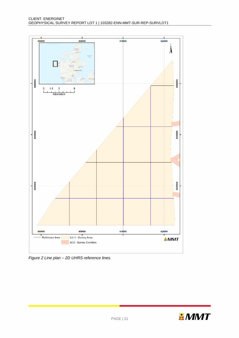
1.8.1| 2D UHRS REFERENCE LINES
Reference lines were surveyed to acquire a representative 2D UHRS seismic dataset of Lot 1. The reference lines were selected form the seismic mainline dataset (4 mainlines and 4 intersecting crosslines). The dataset formed the bases of the first 2D UHRS stratigraphic model used as an interpretation guide for the entire project.
The reference lines were acquired following mobilisation and survey verification, to enable maximum time for review. A framework and strategy was then agreed with the Client prior to further interpretation.
Reference lines are illustrated in Figure 2.
CLIENT: ENERGINET GEOPHYSICAL SURVEY REPORT LOT 1 | 103282-ENN-MMT-SUR-REP-SURVLOT1
PAGE | 21
Figure 2 Line plan – 2D UHRS reference lines.
CLIENT: ENERGINET GEOPHYSICAL SURVEY REPORT LOT 1 | 103282-ENN-MMT-SUR-REP-SURVLOT1
PAGE | 22
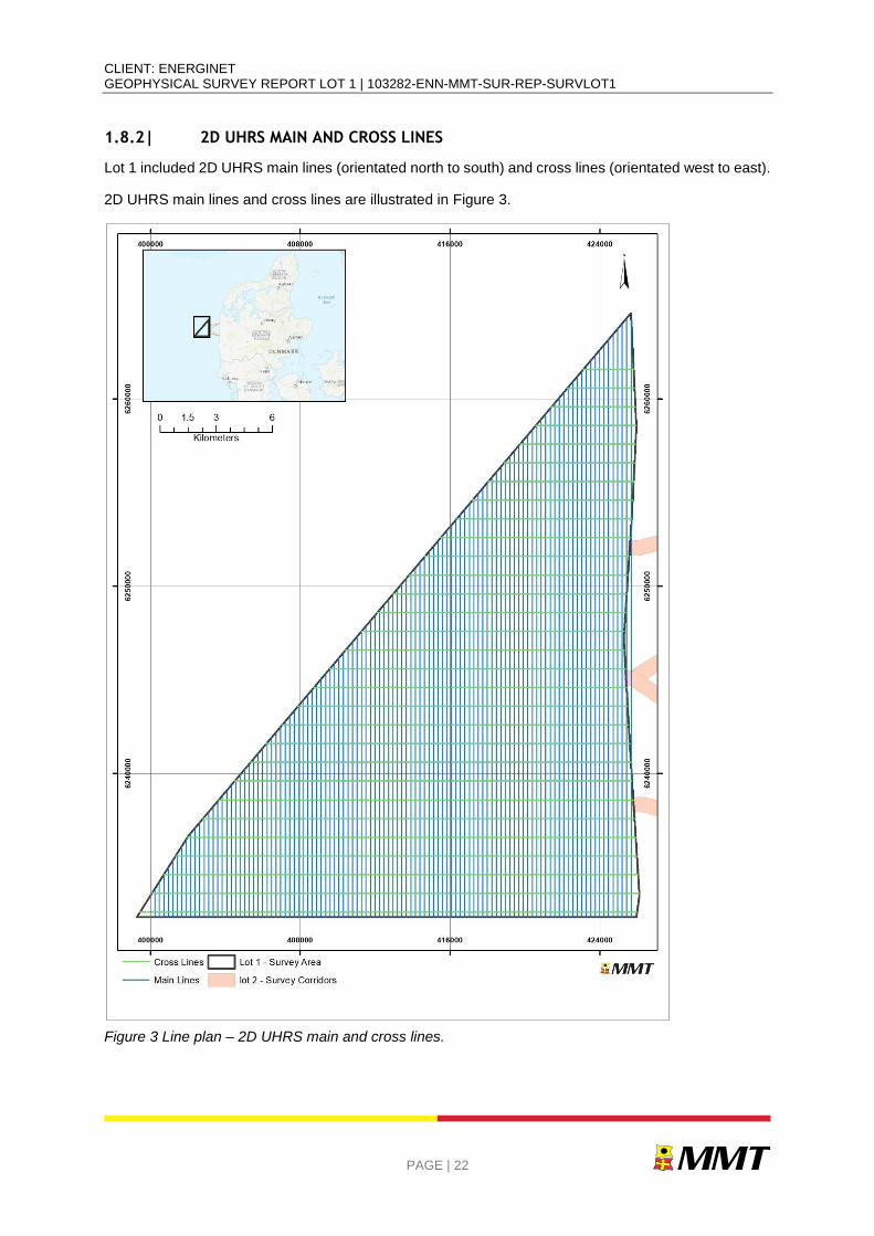
1.8.2| 2D UHRS MAIN AND CROSS LINES
Lot 1 included 2D UHRS main lines (orientated north to south) and cross lines (orientated west to east).
2D UHRS main lines and cross lines are illustrated in Figure 3.
Figure 3 Line plan – 2D UHRS main and cross lines.
CLIENT: ENERGINET GEOPHYSICAL SURVEY REPORT LOT 1 | 103282-ENN-MMT-SUR-REP-SURVLOT1
PAGE | 23
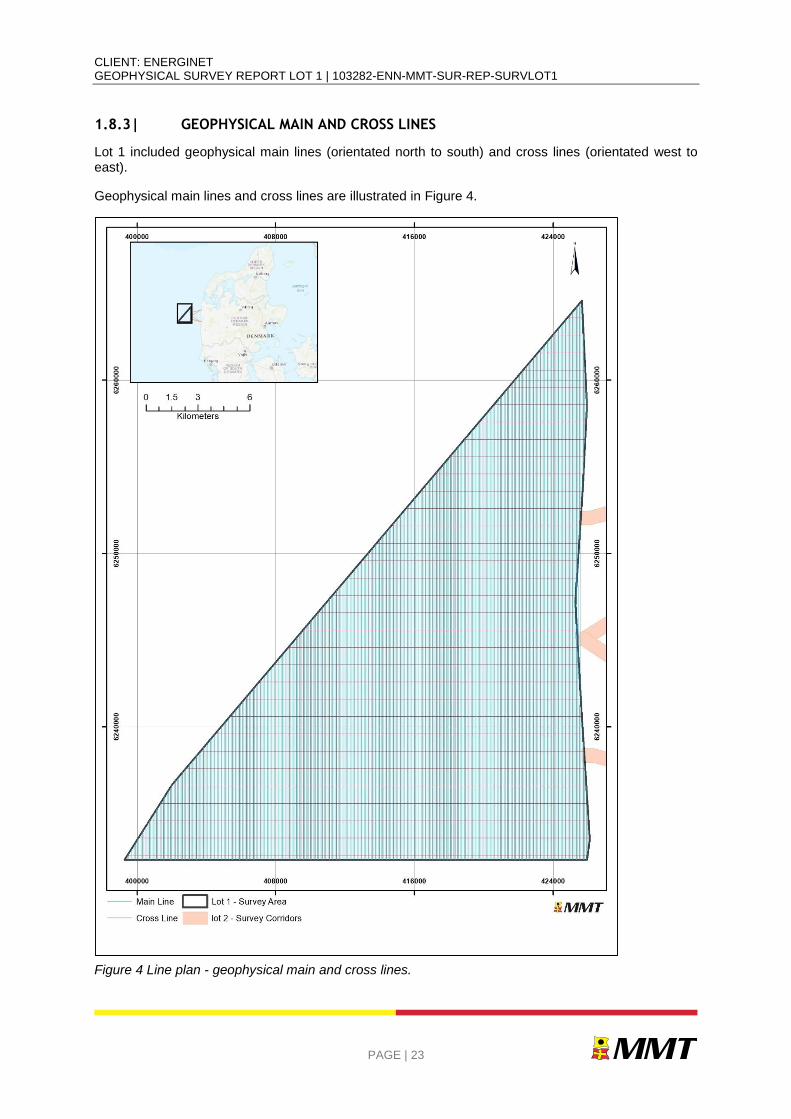
1.8.3| GEOPHYSICAL MAIN AND CROSS LINES
Lot 1 included geophysical main lines (orientated north to south) and cross lines (orientated west to east).
Geophysical main lines and cross lines are illustrated in Figure 4.
Figure 4 Line plan - geophysical main and cross lines.
CLIENT: ENERGINET GEOPHYSICAL SURVEY REPORT LOT 1 | 103282-ENN-MMT-SUR-REP-SURVLOT1
PAGE | 24
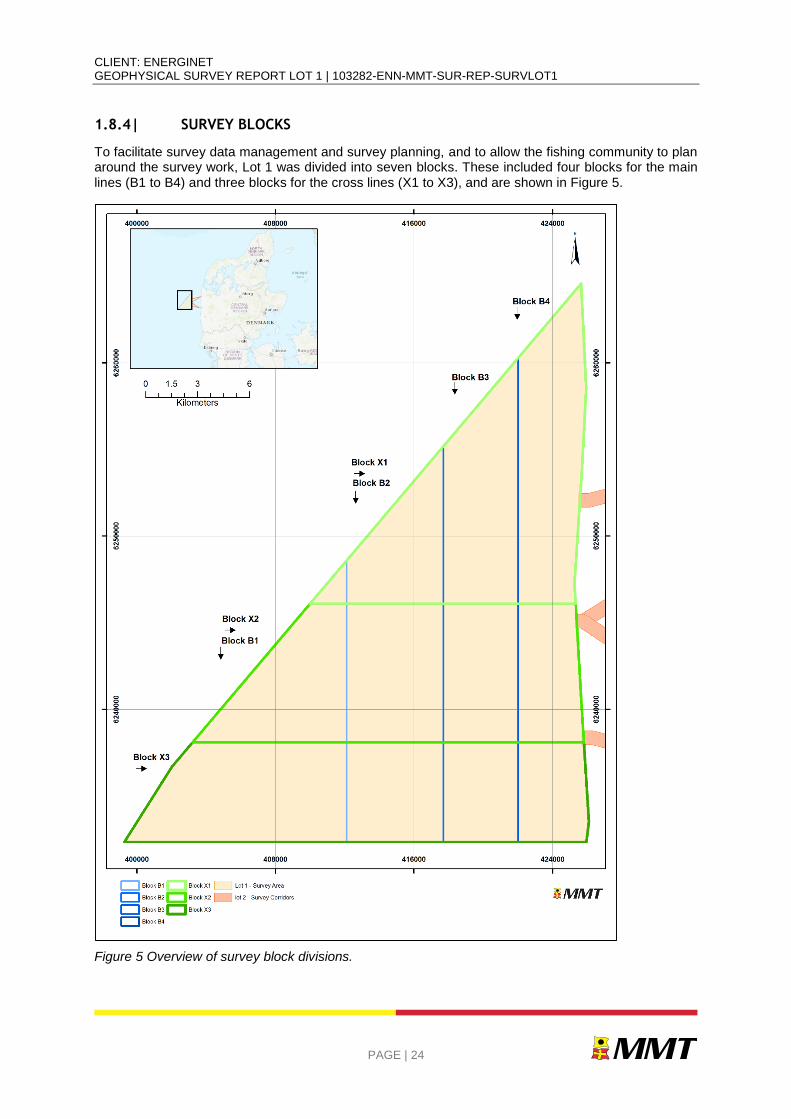
1.8.4| SURVEY BLOCKS
To facilitate survey data management and survey planning, and to allow the fishing community to plan around the survey work, Lot 1 was divided into seven blocks. These included four blocks for the main lines (B1 to B4) and three blocks for the cross lines (X1 to X3), and are shown in Figure 5.
Figure 5 Overview of survey block divisions.
CLIENT: ENERGINET GEOPHYSICAL SURVEY REPORT LOT 1 | 103282-ENN-MMT-SUR-REP-SURVLOT1
PAGE | 25
2| SURVEY PARAMETERS
2.1| GEODETIC DATUM AND GRID COORDINATE SYSTEM
2.1.1| ACQUISITION
The geodetic datum used for survey equipment during acquisition are presented in Table 7.
Table 7 Geodetic parameters used during acquisition.
Horizontal datum: International Terrestrial Reference Frame 2014 (ITRF2014)
Datum ITRF2014
ESPG Datum code 1165
Spheroid Geodetic Reference System 1980 (GRS80)
Semi-major axis 6 378 137.000m
Semi-minor axis 6 356 752.314m
Inverse Flattening (1/f) 298.257222101
2.1.2| PROCESSING
The geodetic datum used during processing and reporting are presented in Table 8.
Table 8 Geodetic parameters used during processing.
Horizontal datum: European Terrestrial Reference System 1989 (ETRS89)
Datum ETRS89
European Petroleum Survey group (EPSG) Datum Code 4936
Spheroid GRS80
Semi-major axis 6 378 137.000m
Semi-minor axis 6 356 752.314m
Inverse Flattening (1/f) 298.257222101
2.1.3| TRANSFORMATION PARAMETERS
The transformation parameters used to covert from acquisition datum (ITRF2014) to processing/reporting datum (ETRS89) are presented in Table 9.
Table 9 Transformation parameters.
DATUM SHIFT FROM ITRF2014 TO ETRS89
(RIGHT-HANDED CONVENTION FOR ROTATION - COORDINATE FRAME ROTATION)
PARAMETERS EPOCH 2019.5
Shift dX (m) +0.099440
Shift dY (m) +0.064160
Shift dZ (m) -0.120400
Rotation rX (“) -.0.00313900
CLIENT: ENERGINET GEOPHYSICAL SURVEY REPORT LOT 1 | 103282-ENN-MMT-SUR-REP-SURVLOT1
PAGE | 26
DATUM SHIFT FROM ITRF2014 TO ETRS89
(RIGHT-HANDED CONVENTION FOR ROTATION - COORDINATE FRAME ROTATION)
Rotation rY (“) -0.01334000
Rotation rZ (“) +0.02369500
Scale Factor (ppm) +0.0030100000
In order to verify that the transformation parameters have been correctly entered into the navigation system the test coordinates supplied in the official transformation document the Simplified transformations from ITRF2014/IGS14 to ETRS89 for maritime applications [L. Jivall, Lantmäteriet, 2018] have been used (Table 10).
Table 10 Official test coordinates Transformation ITRF2014/IGS14, epoch 2019.5 to ETRS89, central Europe
ITRF 2014 epoch 2019.5 54°59’59’’998378 13°29’59.989138 -0.6034
ETRS, central Europe (2019.5) 54°59’59’’980974 13°29’59.958899 -0.6201
ETRS89, Baltic Sea (2019.5) 54°59’59’’981291 13°29’59.958886 -0.6567
SWEREF99, southern Sweden (2019.5) 54°59’59’’981520 13°29’59.959222 -0.6272
2.1.4| PROJECTION PARAMETERS
The projection parameters used for processing and reporting are presented in Table 11.
Table 11 Projection parameters.
Projection Parameters
Projection UTM
Zone 32 N
Central Meridian 09° 00’ 00’’ E
Latitude origin 0
False Northing 0 m
False Easting 500 000 m
Central Scale Factor 0.9996
Units metres
2.1.5| VERTICAL REFERENCE
The vertical reference parameters used for processing and reporting are presented in Table 12.
Table 12 Vertical reference.
Vertical Reference Parameters
Vertical reference MSL
Height model DTU15

CLIENT: ENERGINET GEOPHYSICAL SURVEY REPORT LOT 1 | 103282-ENN-MMT-SUR-REP-SURVLOT1
PAGE | 27
The difference between the vertical height models (DTU15 and DVR90) the OWF are given below in Table 13.
Table 13 Height comparison between DTU15 and DVR90.
ID EASTING NORTHING HEIGHT DTU15 MSL (METRES)
HEIGHT DVR90
MSL (METRES)
DIFFERENCE
(METRES)
OWF Centre 417863.03 6243834.35 40.56 40.65 0.09
2.2| VERTICAL DATUM
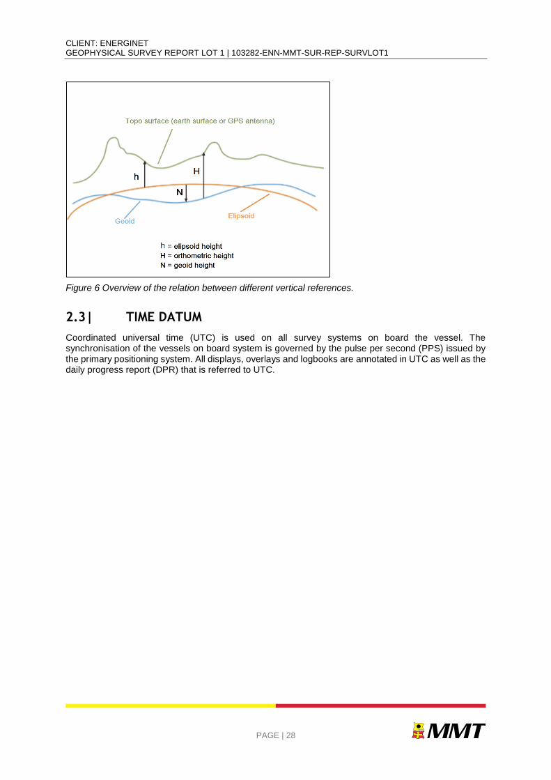
Global navigation satellite system (GNSS) tide was used to reduce the bathymetry data to Mean Sea Level (MSL) the defined vertical reference level (Figure 6). The vertical datum for all depth and/or height measurements was MSL via DTU15 MSL Reduction from WGS84-based ellipsoid heights.
This tidal reduction methodology encompasses all vertical movement of the vessel, including tidal effect and vessel movement due to waves and currents. The short variations in height are identified as heave and the long variations as tide.
This methodology is very robust since it is not limited by the filter settings defined online and provides very good results in complicated mixed wave and swell patterns. The vessel navigation is exported into a post-processed format, Smoothed Best Estimated Trajectory (SBET) that is then applied onto the multibeam echo sounder (MBES) data.
The methodology has proven to be very accurate as it accounts for any changes in height caused by changes in atmospheric pressure, storm surge, squat, loading or any other effect not accounted for in a tidal prediction.
The terms elevation and depth have been used throughout the Lot 1 and Lot 2 reports with the distinction being that elevation refers to a position (or height) above the Mean Sea Level survey datum, with depths being used to refer to positions below the sea surface. Within Lot 1 all positions lie below the sea surface so are referred to in the results section of this report as depths.
Actual numerical values reported are correct with negative values corresponding to sub-sea positions (i.e. depths) and positive values corresponding to subaerial positions (i.e. elevations).
The bathymetric processing software packages EIVA NaviModel and Caris HIPS inherently stores MBES DTMs and sounding data with a positive down depth convention. Report imagery obtained from these packages show the data in this convention. Examples of such images include Figure 60, Figure 65 and Figure 67. For all images from NaviModel and Caris HIPS there will be captions to indicate the reversed depth convention.
CLIENT: ENERGINET GEOPHYSICAL SURVEY REPORT LOT 1 | 103282-ENN-MMT-SUR-REP-SURVLOT1
PAGE | 28
Figure 6 Overview of the relation between different vertical references.
2.3| TIME DATUM
Coordinated universal time (UTC) is used on all survey systems on board the vessel. The synchronisation of the vessels on board system is governed by the pulse per second (PPS) issued by the primary positioning system. All displays, overlays and logbooks are annotated in UTC as well as the daily progress report (DPR) that is referred to UTC.
CLIENT: ENERGINET GEOPHYSICAL SURVEY REPORT LOT 1 | 103282-ENN-MMT-SUR-REP-SURVLOT1
PAGE | 29
3| SURVEY VESSELS
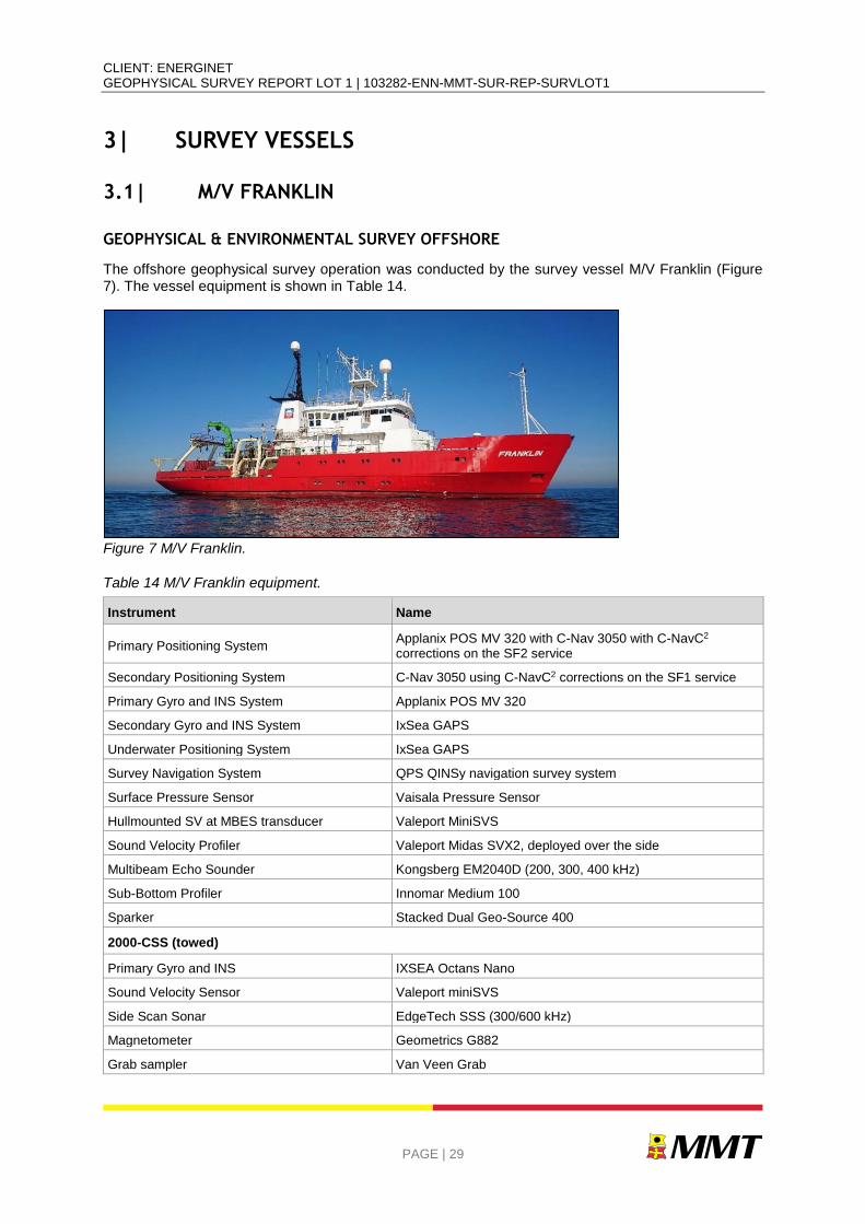
3.1| M/V FRANKLIN
GEOPHYSICAL & ENVIRONMENTAL SURVEY OFFSHORE
The offshore geophysical survey operation was conducted by the survey vessel M/V Franklin (Figure 7). The vessel equipment is shown in Table 14.
Figure 7 M/V Franklin.
Table 14 M/V Franklin equipment.
Instrument Name
Primary Positioning System Applanix POS MV 320 with C-Nav 3050 with C-NavC2 corrections on the SF2 service
Secondary Positioning System C-Nav 3050 using C-NavC2 corrections on the SF1 service
Primary Gyro and INS System Applanix POS MV 320
Secondary Gyro and INS System IxSea GAPS
Underwater Positioning System IxSea GAPS
Survey Navigation System QPS QINSy navigation survey system
Surface Pressure Sensor Vaisala Pressure Sensor
Hullmounted SV at MBES transducer Valeport MiniSVS
Sound Velocity Profiler Valeport Midas SVX2, deployed over the side
Multibeam Echo Sounder Kongsberg EM2040D (200, 300, 400 kHz)
Sub-Bottom Profiler Innomar Medium 100
Sparker Stacked Dual Geo-Source 400
2000-CSS (towed)
Primary Gyro and INS IXSEA Octans Nano
Sound Velocity Sensor Valeport miniSVS
Side Scan Sonar EdgeTech SSS (300/600 kHz)
Magnetometer Geometrics G882
Grab sampler Van Veen Grab
CLIENT: ENERGINET GEOPHYSICAL SURVEY REPORT LOT 1 | 103282-ENN-MMT-SUR-REP-SURVLOT1
PAGE | 30
Instrument Name
ROTV (towed)
Primary Gyro and INS IXSEA ROVINS
Sound Velocity Sensor Valeport miniSVS
Side Scan Sonar EdgeTech SSS (300/600 kHz)
Magnetometer Geometrics G882 (with spare)
3.2| M/V DEEP HELDER
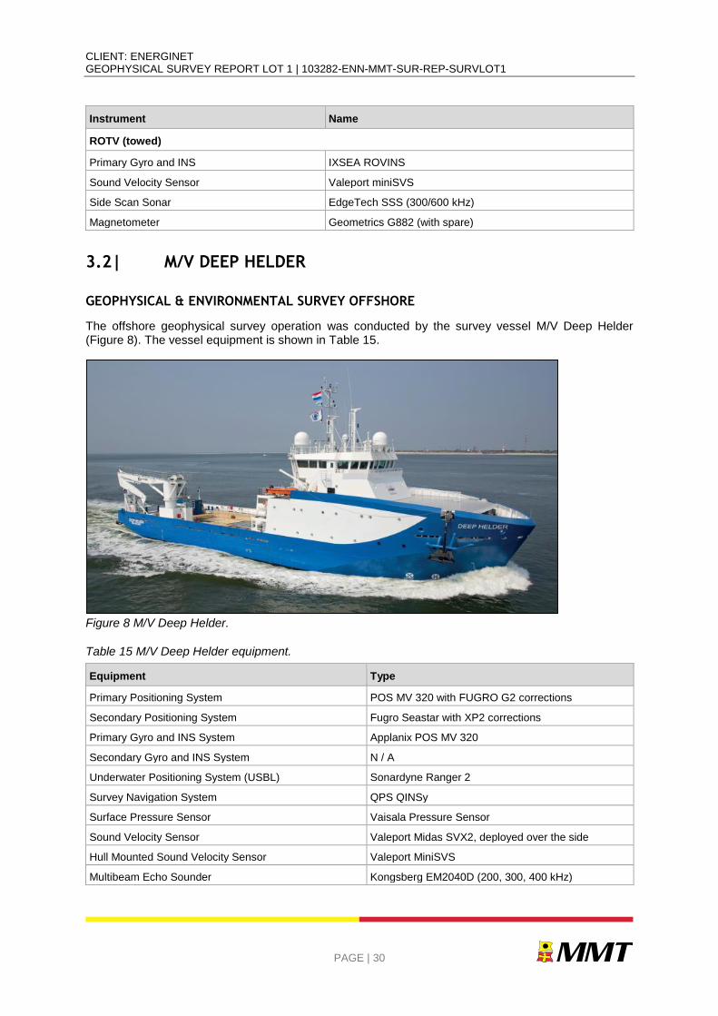
GEOPHYSICAL & ENVIRONMENTAL SURVEY OFFSHORE
The offshore geophysical survey operation was conducted by the survey vessel M/V Deep Helder (Figure 8). The vessel equipment is shown in Table 15.
Figure 8 M/V Deep Helder.
Table 15 M/V Deep Helder equipment.
Equipment Type
Primary Positioning System POS MV 320 with FUGRO G2 corrections
Secondary Positioning System Fugro Seastar with XP2 corrections
Primary Gyro and INS System Applanix POS MV 320
Secondary Gyro and INS System N / A
Underwater Positioning System (USBL) Sonardyne Ranger 2
Survey Navigation System QPS QINSy
Surface Pressure Sensor Vaisala Pressure Sensor
Sound Velocity Sensor Valeport Midas SVX2, deployed over the side
Hull Mounted Sound Velocity Sensor Valeport MiniSVS
Multibeam Echo Sounder Kongsberg EM2040D (200, 300, 400 kHz)
CLIENT: ENERGINET GEOPHYSICAL SURVEY REPORT LOT 1 | 103282-ENN-MMT-SUR-REP-SURVLOT1
PAGE | 31
Equipment Type
Sub-Bottom Profiler Innomar SES2000
2000-CSS (towed)
Sound Velocity Sensor Valeport miniSVS
Side Scan Sonar EdgeTech SSS (300/600 kHz)
Magnetometer Geometrics G882
3.3| M/V STRIL EXPLORER
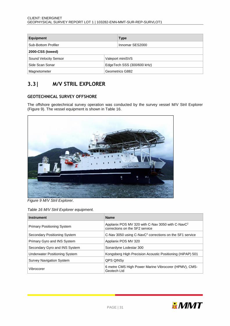
GEOTECHNICAL SURVEY OFFSHORE
The offshore geotechnical survey operation was conducted by the survey vessel M/V Stril Explorer (Figure 9). The vessel equipment is shown in Table 16.
Figure 9 M/V Stril Explorer.
Table 16 M/V Stril Explorer equipment.
Instrument Name
Primary Positioning System Applanix POS MV 320 with C-Nav 3050 with C-NavC2 corrections on the SF2 service
Secondary Positioning System C-Nav 3050 using C-NavC2 corrections on the SF1 service
Primary Gyro and INS System Applanix POS MV 320
Secondary Gyro and INS System Sonardyne Lodestar 300
Underwater Positioning System Kongsberg High Precision Acoustic Positioning (HiPAP) 501
Survey Navigation System QPS QINSy
Vibrocorer 6 metre CMS High Power Marine Vibrocorer (HPMV), CMS-Geotech Ltd
CLIENT: ENERGINET GEOPHYSICAL SURVEY REPORT LOT 1 | 103282-ENN-MMT-SUR-REP-SURVLOT1
PAGE | 32
4| DATA PROCESSING AND INTERPRETATION METHODS
4.1| BATHYMETRY
The objective of the processing workflow is to create a Digital Terrain Model (DTM) that provides the most realistic representation of the seabed with the highest possible detail. The processing scheme for MBES data comprised two main scopes: horizontal and vertical levelling in order to homogenise the dataset and data cleaning in order to remove outliers.
The MBES data is initially brought into Caris HIPS to check that it has met the coverage and density requirements. It then has a post-processed navigation solution applied in the form of a SBET. The SBET was created by using post-processed navigation and attitude derived primarily from the POS M/V Inertial Measurement Unit (IMU) data records. This data is processed in POSPac MMS and then applied to the project in Caris HIPS.
In addition to the updated position data, a file containing the positional error data for each SBET is also applied to the associated MBES data. The positional error data exported from POSPac MMS contributes to the Total Horizontal Uncertainty (THU) and Total Vertical Uncertainty (TVU) which is computed for each sounding within the dataset. These surfaces are generated in Caris HIPS and are checked for deviations from the THU and TVU thresholds as specified by the client. This is discussed in further detail in Section 5.1|.
After the post-processed position and error data is applied, a Global Navigation Satellite System (GNSS) tide is calculated from the SBET altitude data which vertically corrects the bathymetry using the DTU15 MSL to GRS80 Ellipsoidal Separation model within Caris HIPS. The bathymetry data for each processed MBES data file is then merged together to create a homogenised surface which can be reviewed for both standard deviation and sounding density. Once the data has passed these checks it is ready to start the process of removing outlying soundings which can be undertaken within Caris HIPS or in EIVA NaviModel.
In the Caris HIPS workflow an average surface is derived from the sounding data and from this it is possible to remove outliers that lie at a specified numerical distance from the surface, or by setting a standard deviation threshold. Manual cleaning can also be performed using the Subset Editor tool to clean areas around features that would be liable to being removed by the automatic cleaning processes.
In the EIVA NaviModel workflow the data is turned into a 3D model which undergoes further checks and data cleaning processes. Typically, a Scalgo Combinatorial Anti-Noise (S-CAN) filter is applied to the data to remove any outliers although some manual cleaning may also take place. This data cleaning is then written back to the data in the Caris HIPS project ready for Quality Check (QC).
In Caris HIPS the QC surfaces are recalculated to integrate any sounding flag editing that has occurred in NaviModel or within HIPS and examined to check that the dataset complies with the project specification. If the dataset passes this QC check then products (DTMs, contours and shaded images) can be exported from either Caris HIPS or NaviModel for delivery or for further internal use.
The work flow diagram for MBES processing is shown in Figure 10.
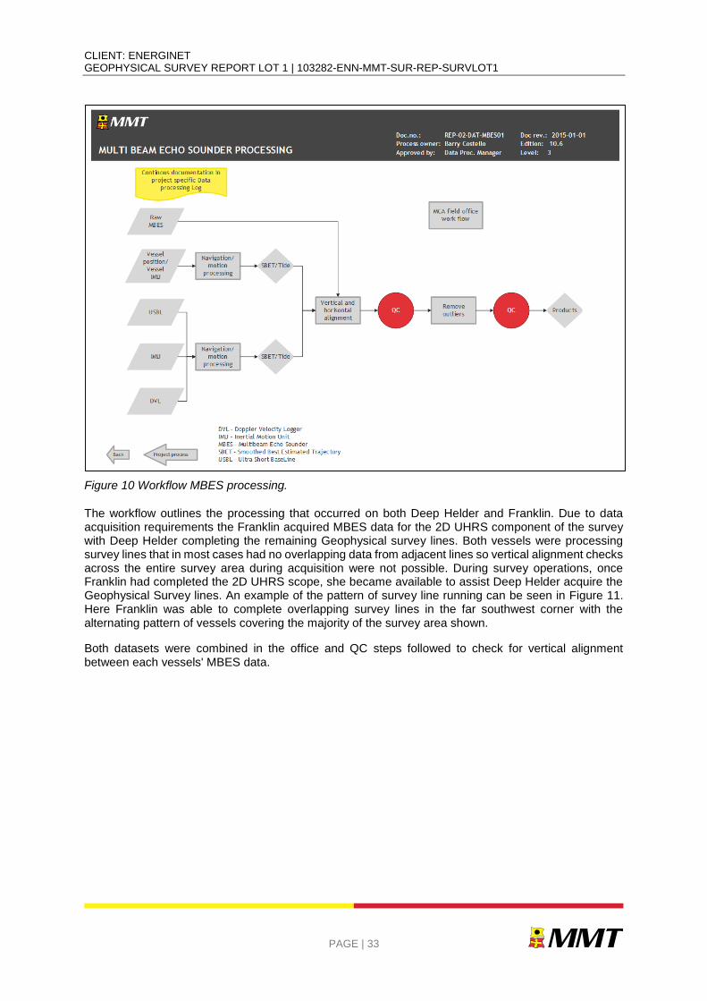
CLIENT: ENERGINET GEOPHYSICAL SURVEY REPORT LOT 1 | 103282-ENN-MMT-SUR-REP-SURVLOT1
PAGE | 33
Figure 10 Workflow MBES processing.
The workflow outlines the processing that occurred on both Deep Helder and Franklin. Due to data acquisition requirements the Franklin acquired MBES data for the 2D UHRS component of the survey with Deep Helder completing the remaining Geophysical survey lines. Both vessels were processing survey lines that in most cases had no overlapping data from adjacent lines so vertical alignment checks across the entire survey area during acquisition were not possible. During survey operations, once Franklin had completed the 2D UHRS scope, she became available to assist Deep Helder acquire the Geophysical Survey lines. An example of the pattern of survey line running can be seen in Figure 11. Here Franklin was able to complete overlapping survey lines in the far southwest corner with the alternating pattern of vessels covering the majority of the survey area shown.
Both datasets were combined in the office and QC steps followed to check for vertical alignment between each vessels' MBES data.
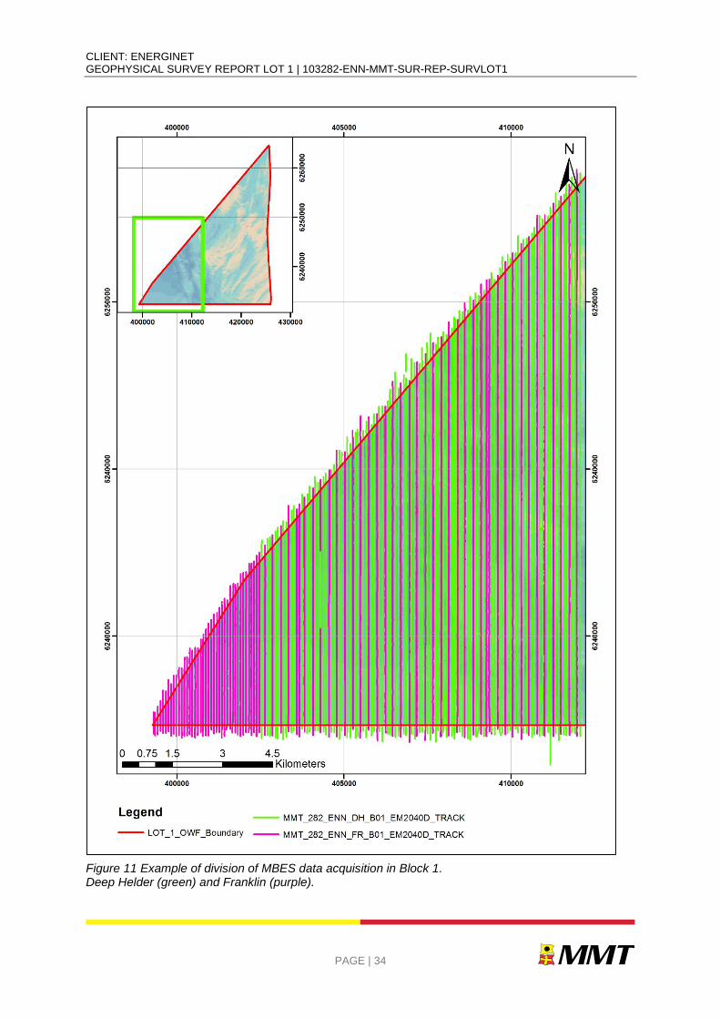
CLIENT: ENERGINET GEOPHYSICAL SURVEY REPORT LOT 1 | 103282-ENN-MMT-SUR-REP-SURVLOT1
PAGE | 34
Figure 11 Example of division of MBES data acquisition in Block 1. Deep Helder (green) and Franklin (purple).
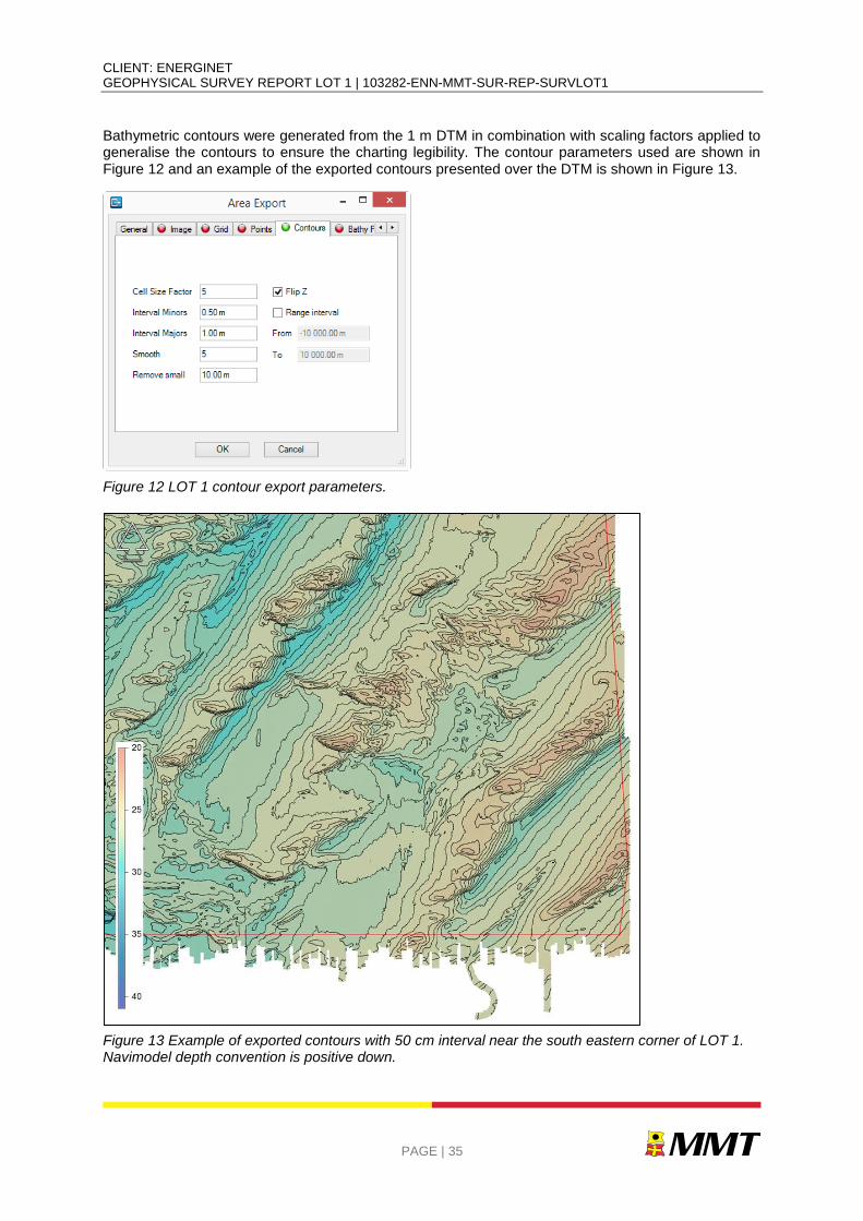
CLIENT: ENERGINET GEOPHYSICAL SURVEY REPORT LOT 1 | 103282-ENN-MMT-SUR-REP-SURVLOT1
PAGE | 35
Bathymetric contours were generated from the 1 m DTM in combination with scaling factors applied to generalise the contours to ensure the charting legibility. The contour parameters used are shown in Figure 12 and an example of the exported contours presented over the DTM is shown in Figure 13.
Figure 12 LOT 1 contour export parameters.
Figure 13 Example of exported contours with 50 cm interval near the south eastern corner of LOT 1. Navimodel depth convention is positive down.
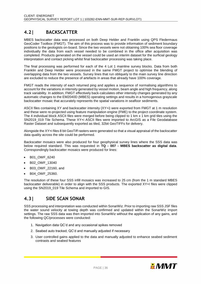
CLIENT: ENERGINET GEOPHYSICAL SURVEY REPORT LOT 1 | 103282-ENN-MMT-SUR-REP-SURVLOT1
PAGE | 36
4.2| BACKSCATTER
MBES backscatter data was processed on both Deep Helder and Franklin using QPS Fledermaus GeoCoder Toolbox (FMGT). The aim of this process was to provide information of sediment boundary positions to the geologists on-board. Since the two vessels were not obtaining 100% sea floor coverage individually the data from each vessel needed to be combined in the office after acquisition was completed. Products generated on the vessel could be used an interim dataset for the surficial geology interpretation and contact picking whilst final backscatter processing was taking place.
The final processing was performed for each of the 4 Lot 1 mainline survey blocks. Data from both Franklin and Deep Helder were processed in the same FMGT project to optimise the blending of overlapping data from the two vessels. Survey lines that run obliquely to the main survey line direction are excluded to reduce the presence of artefacts in areas that already have 100% coverage.
FMGT reads the intensity of each returned ping and applies a sequence of normalising algorithms to account for the variations in intensity generated by vessel motion, beam angle and high frequency, along track variability. In addition, FMGT effectively back-calculates other intensity changes generated by any automatic changes to the EM2040D (MBES) operating settings and results in a homogenous grayscale backscatter mosaic that accurately represents the spatial variations in seafloor sediments.
ASCII files containing XY and backscatter intensity (XY+i) were exported from FMGT at 1 m resolution and these were re-projected using feature manipulation engine (FME) to the project coordinate system. The 4 individual block ASCII files were merged before being clipped to 1 km x 1 km grid tiles using the SN2019_019 Tile Schema. These XY+i ASCII files were imported to ArcGIS as a File Geodatabase Raster Dataset and subsequently exported as tiled, 32bit GeoTIFFs for delivery.
Alongside the XY+i files 8 bit GeoTiff rasters were generated so that a visual appraisal of the backscatter data quality across the site could be performed.
Backscatter mosaics were also produced for four geophysical survey lines where the SSS data was below required standard. This was requested in TQ - 007 - MBES backscatter as digital data.
Correspondingly backscatter mosaics were produced for lines:
B01_OWF_6240
B02_OWF_13040
B03_OWF_22160, and
B04_OWF_25360.
The resolution of these four SSS infill mosaics was increased to 25 cm (from the 1 m standard MBES backscatter deliverable) in order to align with the SSS products. The exported XY+I files were clipped using the SN2019_019 Tile Schema and imported to GIS.
4.3| SIDE SCAN SONAR
SSS processing and interpretation was conducted within SonarWiz. Prior to importing raw SSS JSF files the water sound velocity at towing depth was confirmed and updated within the SonarWiz import settings. The raw SSS data was then imported into SonarWiz without the application of any gains, and the following QC/processes were conducted:
1. Navigation data QC’d and any occasional spikes removed
2. Seabed auto tracked, QC’d and manually adjusted if necessary
3. User controlled gains applied to the data and manually adjusted to enhance seabed sediment contrasts and seabed features

CLIENT: ENERGINET GEOPHYSICAL SURVEY REPORT LOT 1 | 103282-ENN-MMT-SUR-REP-SURVLOT1
PAGE | 37
4. SSS data QC’d against MBES data by locating features/contacts clearly distinguishable in both data sets and comparing appearance and position
5. Coverage QC’d and any gaps flagged and infilled in order to meet client coverage requirements
The SSS processing workflow is outlined in Figure 14 and Figure 15.
The processing was conducted with the following objectives:
To classify seabed surface sediments
To classify mobile bedforms and other potential hazards
To identify natural and anthropogenic seabed features
To detect contacts
To detect cables and pipelines
The interpretation of SSS geo-boundaries was conducted within SonarWiz and AutoCAD software. Within SonarWiz geo-boundaries were digitised as features and exported as DXF files. For digitisation in AutoCAD, SSS mosaics were exported from SonarWiz loaded into AutoCAD and line and polygon features mapped. Before the mosaic were exported as a geotiffs, the files were arranged so the best available data is uppermost. The nadir was made transparent in order for data in overlapping files that cover the nadir gap to be seen. This process is conducted for both high frequency (HF) and low frequency (LF) data sets.
Once the mosaics were exported from SonarWiz, they were organized in FME, in 1km tiles following the Universal Transverse Mercator (UTM) grid on the area.
The geo-boundaries were reviewed against backscatter, MBES and magnetometer (MAG) grid data so an integrated interpretation was obtained based upon all available data. Seabed sediment classifications were also reconciled against the geotechnical grab sample (GS) and vibrocorer (VC) results. Interpretations were QC’d and finalised by a Senior Geologist.
The interpretation of SSS contacts was conducted within SonarWiz. The SSS data was viewed in digitising mode and contacts were selected according to specifications. Wrecks/cables were correlated to existing databases. Contacts were digitised alongside MBES data so that associations with a visible MBES feature could be included within the comments, and to ensure that all contacts visible on the MBES data were identified by the SSS. The interpreted contacts were QC’d and correlation/assessment against MBES data repeated by a different geologist to the one who completed the original interpretation, and a list of accepted contacts created. The contacts list was then correlated to MAG.
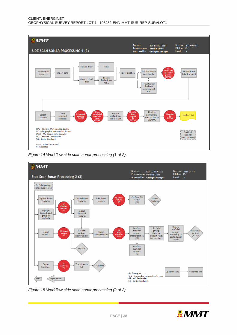
CLIENT: ENERGINET GEOPHYSICAL SURVEY REPORT LOT 1 | 103282-ENN-MMT-SUR-REP-SURVLOT1
PAGE | 38
Figure 14 Workflow side scan sonar processing (1 of 2).
Figure 15 Workflow side scan sonar processing (2 of 2).
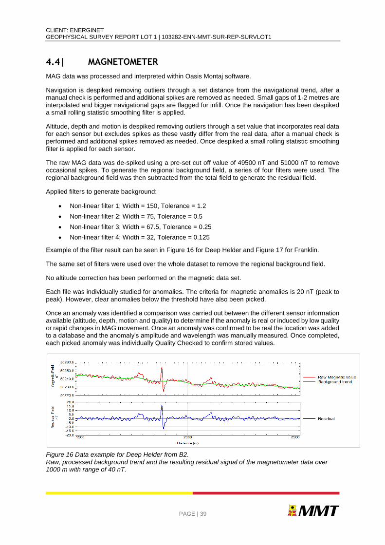
CLIENT: ENERGINET GEOPHYSICAL SURVEY REPORT LOT 1 | 103282-ENN-MMT-SUR-REP-SURVLOT1
PAGE | 39
4.4| MAGNETOMETER
MAG data was processed and interpreted within Oasis Montaj software.
Navigation is despiked removing outliers through a set distance from the navigational trend, after a manual check is performed and additional spikes are removed as needed. Small gaps of 1-2 metres are interpolated and bigger navigational gaps are flagged for infill. Once the navigation has been despiked a small rolling statistic smoothing filter is applied.
Altitude, depth and motion is despiked removing outliers through a set value that incorporates real data for each sensor but excludes spikes as these vastly differ from the real data, after a manual check is performed and additional spikes removed as needed. Once despiked a small rolling statistic smoothing filter is applied for each sensor.
The raw MAG data was de-spiked using a pre-set cut off value of 49500 nT and 51000 nT to remove occasional spikes. To generate the regional background field, a series of four filters were used. The regional background field was then subtracted from the total field to generate the residual field.
Applied filters to generate background:
Non-linear filter 1; Width = 150, Tolerance = 1.2
Non-linear filter 2; Width = 75, Tolerance = 0.5
Non-linear filter 3; Width = 67.5, Tolerance = 0.25
Non-linear filter 4; Width = 32, Tolerance = 0.125
Example of the filter result can be seen in Figure 16 for Deep Helder and Figure 17 for Franklin.
The same set of filters were used over the whole dataset to remove the regional background field.
No altitude correction has been performed on the magnetic data set.
Each file was individually studied for anomalies. The criteria for magnetic anomalies is 20 nT (peak to peak). However, clear anomalies below the threshold have also been picked.
Once an anomaly was identified a comparison was carried out between the different sensor information available (altitude, depth, motion and quality) to determine if the anomaly is real or induced by low quality or rapid changes in MAG movement. Once an anomaly was confirmed to be real the location was added to a database and the anomaly’s amplitude and wavelength was manually measured. Once completed, each picked anomaly was individually Quality Checked to confirm stored values.
Figure 16 Data example for Deep Helder from B2. Raw, processed background trend and the resulting residual signal of the magnetometer data over 1000 m with range of 40 nT.
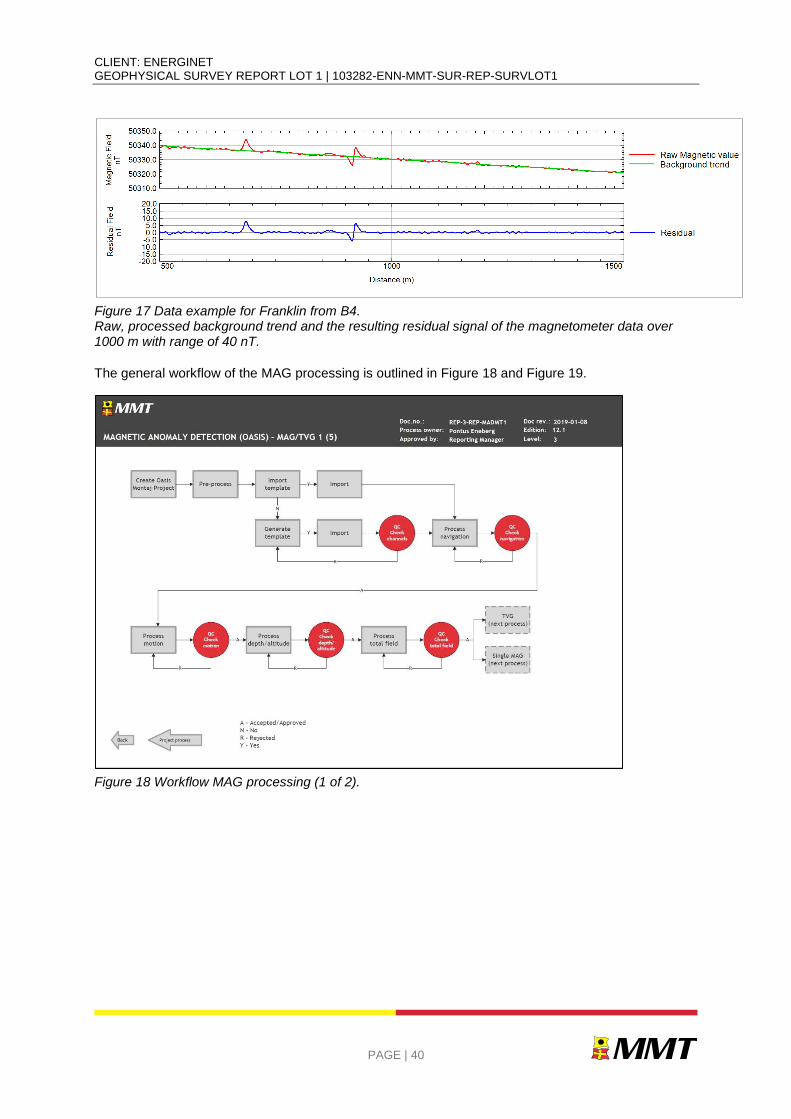
CLIENT: ENERGINET GEOPHYSICAL SURVEY REPORT LOT 1 | 103282-ENN-MMT-SUR-REP-SURVLOT1
PAGE | 40
Figure 17 Data example for Franklin from B4. Raw, processed background trend and the resulting residual signal of the magnetometer data over 1000 m with range of 40 nT.
The general workflow of the MAG processing is outlined in Figure 18 and Figure 19.
Figure 18 Workflow MAG processing (1 of 2).
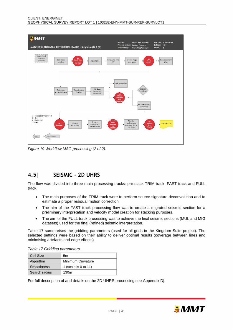
CLIENT: ENERGINET GEOPHYSICAL SURVEY REPORT LOT 1 | 103282-ENN-MMT-SUR-REP-SURVLOT1
PAGE | 41
Figure 19 Workflow MAG processing (2 of 2).
4.5| SEISMIC - 2D UHRS
The flow was divided into three main processing tracks: pre-stack TRIM track, FAST track and FULL track.
The main purposes of the TRIM track were to perform source signature deconvolution and to estimate a proper residual motion correction.
The aim of the FAST track processing flow was to create a migrated seismic section for a preliminary interpretation and velocity model creation for stacking purposes.
The aim of the FULL track processing was to achieve the final seismic sections (MUL and MIG datasets) used for the final (refined) seismic interpretation.
Table 17 summarises the gridding parameters (used for all grids in the Kingdom Suite project). The selected settings were based on their ability to deliver optimal results (coverage between lines and minimising artefacts and edge effects).
Table 17 Gridding parameters.
Cell Size 5m
Algorithm Minimum Curvature
Smoothness 1 (scale is 0 to 11)
Search radius 130m
For full description of and details on the 2D UHRS processing see Appendix D|.
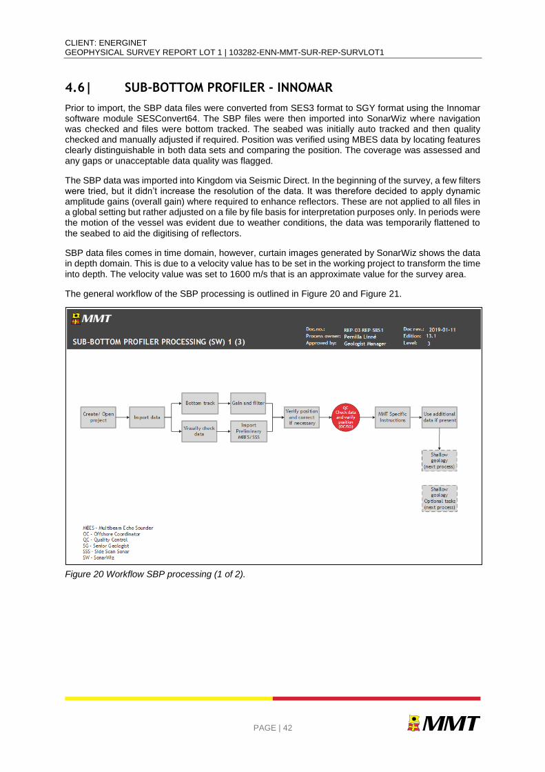
CLIENT: ENERGINET GEOPHYSICAL SURVEY REPORT LOT 1 | 103282-ENN-MMT-SUR-REP-SURVLOT1
PAGE | 42
4.6| SUB-BOTTOM PROFILER - INNOMAR
Prior to import, the SBP data files were converted from SES3 format to SGY format using the Innomar software module SESConvert64. The SBP files were then imported into SonarWiz where navigation was checked and files were bottom tracked. The seabed was initially auto tracked and then quality checked and manually adjusted if required. Position was verified using MBES data by locating features clearly distinguishable in both data sets and comparing the position. The coverage was assessed and any gaps or unacceptable data quality was flagged.
The SBP data was imported into Kingdom via Seismic Direct. In the beginning of the survey, a few filters were tried, but it didn’t increase the resolution of the data. It was therefore decided to apply dynamic amplitude gains (overall gain) where required to enhance reflectors. These are not applied to all files in a global setting but rather adjusted on a file by file basis for interpretation purposes only. In periods were the motion of the vessel was evident due to weather conditions, the data was temporarily flattened to the seabed to aid the digitising of reflectors.
SBP data files comes in time domain, however, curtain images generated by SonarWiz shows the data in depth domain. This is due to a velocity value has to be set in the working project to transform the time into depth. The velocity value was set to 1600 m/s that is an approximate value for the survey area.
The general workflow of the SBP processing is outlined in Figure 20 and Figure 21.
Figure 20 Workflow SBP processing (1 of 2).
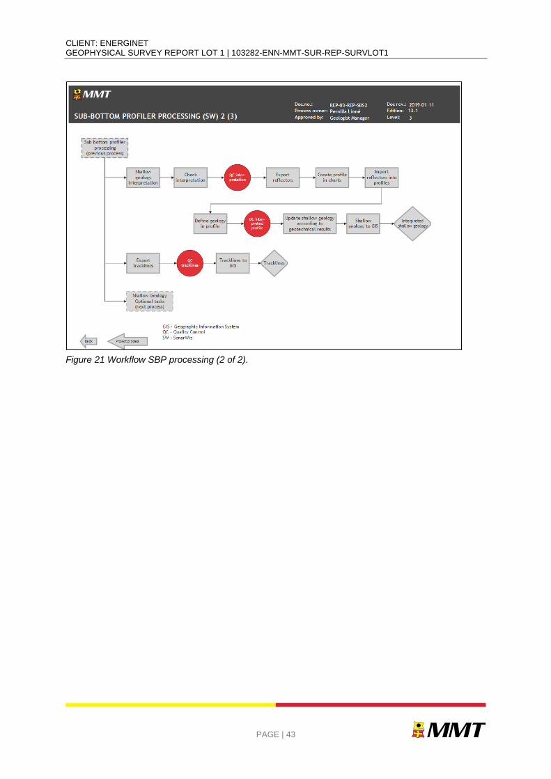
CLIENT: ENERGINET GEOPHYSICAL SURVEY REPORT LOT 1 | 103282-ENN-MMT-SUR-REP-SURVLOT1
PAGE | 43
Figure 21 Workflow SBP processing (2 of 2).
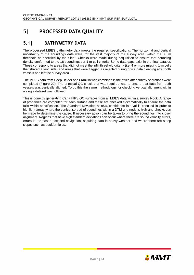
CLIENT: ENERGINET GEOPHYSICAL SURVEY REPORT LOT 1 | 103282-ENN-MMT-SUR-REP-SURVLOT1
PAGE | 44
5| PROCESSED DATA QUALITY
5.1| BATHYMETRY DATA
The processed MBES bathymetry data meets the required specifications. The horizontal and vertical uncertainty of the soundings data were, for the vast majority of the survey area, within the 0.5 m threshold as specified by the client. Checks were made during acquisition to ensure that sounding density conformed to the 16 soundings per 1 m cell criteria. Some data gaps exist in the final dataset. These correspond to areas that did not meet the infill threshold criteria (i.e. 4 or more missing 1 m cells that shared a long side) and areas that were flagged as rejected during office data cleaning after both vessels had left the survey area.
The MBES data from Deep Helder and Franklin was combined in the office after survey operations were completed (Figure 22). The principal QC check that was required was to ensure that data from both vessels was vertically aligned. To do this the same methodology for checking vertical alignment within a single dataset was followed.
This is done by generating Caris HIPS QC surfaces from all MBES data within a survey block. A range of properties are computed for each surface and these are checked systematically to ensure the data falls within specification. The Standard Deviation at 95% confidence interval is checked in order to highlight areas where the vertical spread of soundings within a DTM grid node is high and checks can be made to determine the cause. If necessary action can be taken to bring the soundings into closer alignment. Regions that have high standard deviations can occur where there are sound velocity errors, errors in the post-processed navigation, acquiring data in heavy weather and where there are steep slopes such as boulder fields.
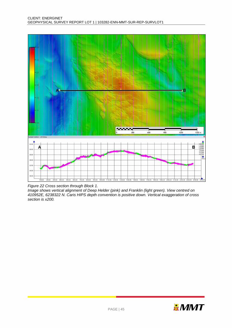
CLIENT: ENERGINET GEOPHYSICAL SURVEY REPORT LOT 1 | 103282-ENN-MMT-SUR-REP-SURVLOT1
PAGE | 45
Figure 22 Cross section through Block 1. Image shows vertical alignment of Deep Helder (pink) and Franklin (light green). View centred on 410952E, 6238322 N. Caris HIPS depth convention is positive down. Vertical exaggeration of cross section is x200.
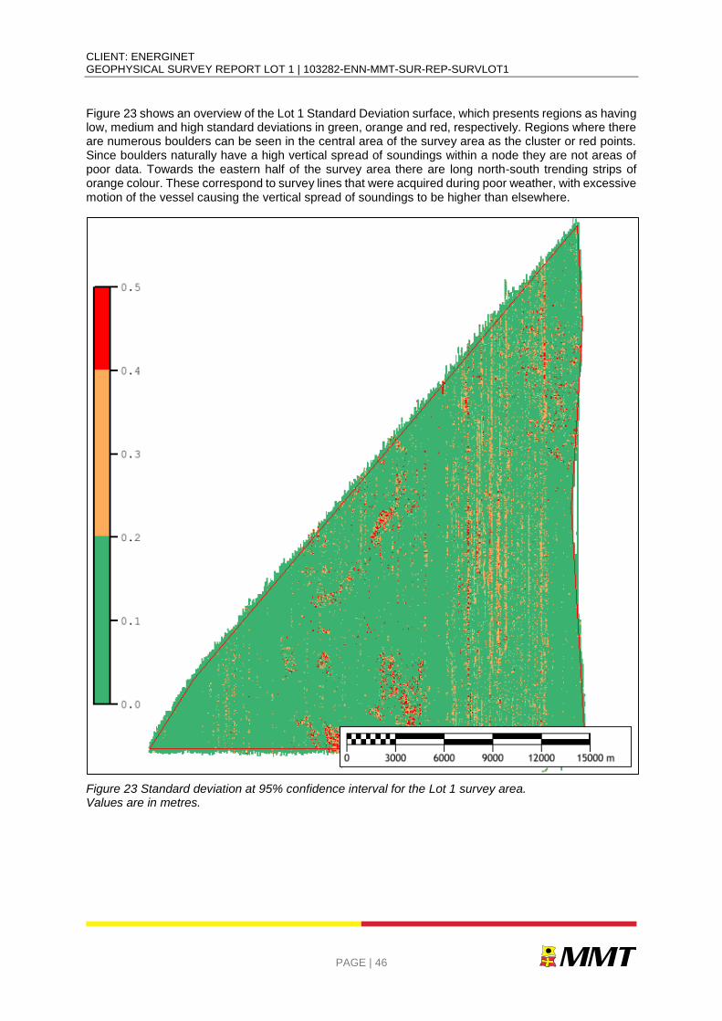
CLIENT: ENERGINET GEOPHYSICAL SURVEY REPORT LOT 1 | 103282-ENN-MMT-SUR-REP-SURVLOT1
PAGE | 46
Figure 23 shows an overview of the Lot 1 Standard Deviation surface, which presents regions as having low, medium and high standard deviations in green, orange and red, respectively. Regions where there are numerous boulders can be seen in the central area of the survey area as the cluster or red points. Since boulders naturally have a high vertical spread of soundings within a node they are not areas of poor data. Towards the eastern half of the survey area there are long north-south trending strips of orange colour. These correspond to survey lines that were acquired during poor weather, with excessive motion of the vessel causing the vertical spread of soundings to be higher than elsewhere.
Figure 23 Standard deviation at 95% confidence interval for the Lot 1 survey area. Values are in metres.
CLIENT: ENERGINET GEOPHYSICAL SURVEY REPORT LOT 1 | 103282-ENN-MMT-SUR-REP-SURVLOT1
PAGE | 47
Figure 24 and Figure 25 provide examples of the standard deviation surface and cross sections through the soundings data for periods of good weather and poor weather. Figure 24 shows a region with low standarad deviation in the south eastern part of Block 1. This highly exaggerated cross section shows that MV Franklin and MV Deep Helder produced data that was well aligned and displays a similar vertical spread of soundings. Figure 25 shows a region within Block 03 which has variable standard deviation which results from poor weather during the period of MV Deep Helder's acquisition. In the cross section the MV Franklin data shows a tighter vertical spread of data than the contribution from MV Deep Helder. The region of the Lot 1 survey area nearer to shore was worked in during periods when weather was too poor to work in areas further west but not sufficiently bad that the vessels had to return to port to wait for better conditions.
Figure 24 Example of MBES data acquired during good weather with a similar vertical spread of soundings for MV Franklin and MV Deep Helder. Soundings from MV Franklin shown in green and MV Deep Helder in pink. The yellow bar marks the location of the cross section in lower half of image. Caris HIPS depth convention is positive down, vertical exaggeration of cross section is x100.
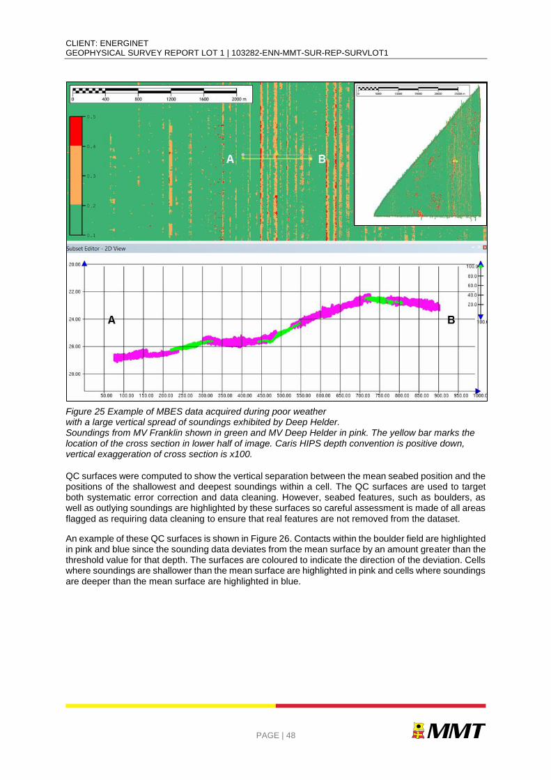
CLIENT: ENERGINET GEOPHYSICAL SURVEY REPORT LOT 1 | 103282-ENN-MMT-SUR-REP-SURVLOT1
PAGE | 48
Figure 25 Example of MBES data acquired during poor weather with a large vertical spread of soundings exhibited by Deep Helder. Soundings from MV Franklin shown in green and MV Deep Helder in pink. The yellow bar marks the location of the cross section in lower half of image. Caris HIPS depth convention is positive down, vertical exaggeration of cross section is x100.
QC surfaces were computed to show the vertical separation between the mean seabed position and the positions of the shallowest and deepest soundings within a cell. The QC surfaces are used to target both systematic error correction and data cleaning. However, seabed features, such as boulders, as well as outlying soundings are highlighted by these surfaces so careful assessment is made of all areas flagged as requiring data cleaning to ensure that real features are not removed from the dataset.
An example of these QC surfaces is shown in Figure 26. Contacts within the boulder field are highlighted in pink and blue since the sounding data deviates from the mean surface by an amount greater than the threshold value for that depth. The surfaces are coloured to indicate the direction of the deviation. Cells where soundings are shallower than the mean surface are highlighted in pink and cells where soundings are deeper than the mean surface are highlighted in blue.
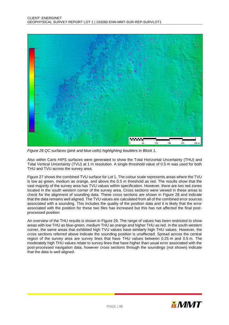
CLIENT: ENERGINET GEOPHYSICAL SURVEY REPORT LOT 1 | 103282-ENN-MMT-SUR-REP-SURVLOT1
PAGE | 49
Figure 26 QC surfaces (pink and blue cells) highlighting boulders in Block 1.
Also within Caris HIPS surfaces were generated to show the Total Horizontal Uncertainty (THU) and Total Vertical Uncertainty (TVU) at 1 m resolution. A single threshold value of 0.5 m was used for both THU and TVU across the survey area.
Figure 27 shows the combined TVU surface for Lot 1. The colour scale represents areas where the TVU is low as green, medium as orange, and above the 0.5 m threshold as red. The results show that the vast majority of the survey area has TVU values within specification. However, there are two red zones located in the south western corner of the survey area. Cross sections were viewed in these areas to check for the alignment of sounding data. These cross sections are shown in Figure 28 and indicate that the data remains well aligned. The TVU values are calculated from all of the combined error sources associated with a sounding. This includes the quality of the position data and it is likely that the error associated with the position for these two files has increased but this has not affected the final post-processed position.
An overview of the THU results is shown in Figure 29. The range of values has been restricted to show areas with low THU as blue-green, medium THU as orange and higher THU as red. In the south western corner, the same areas that exhibited high TVU values have similarly high THU values. However, the cross sections referred above indicate the sounding position is unaffected. Spread across the central region of the survey area are survey lines that have THU values between 0.25 m and 0.5 m. The moderately high THU values relate to survey lines that have higher than usual error associated with the post-processed navigation data, however cross sections through the soundings (not shown) indicate that the data is well aligned.
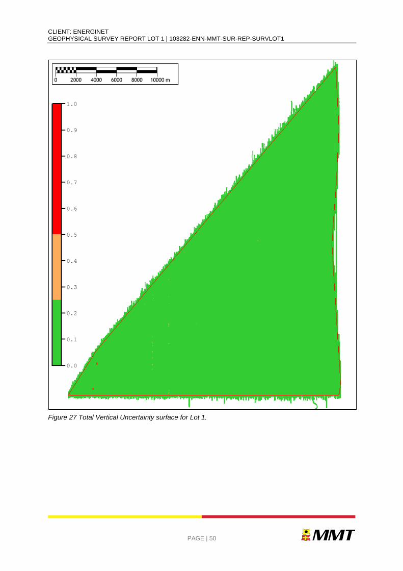
CLIENT: ENERGINET GEOPHYSICAL SURVEY REPORT LOT 1 | 103282-ENN-MMT-SUR-REP-SURVLOT1
PAGE | 50
Figure 27 Total Vertical Uncertainty surface for Lot 1.
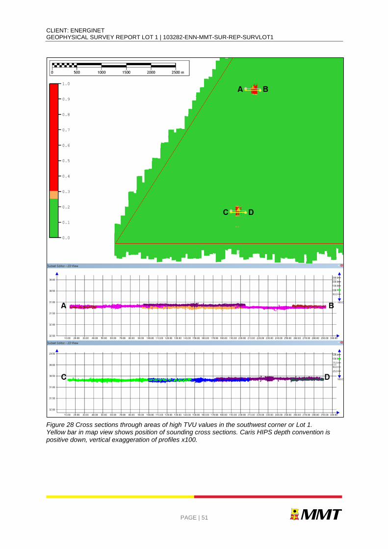
CLIENT: ENERGINET GEOPHYSICAL SURVEY REPORT LOT 1 | 103282-ENN-MMT-SUR-REP-SURVLOT1
PAGE | 51
Figure 28 Cross sections through areas of high TVU values in the southwest corner or Lot 1. Yellow bar in map view shows position of sounding cross sections. Caris HIPS depth convention is positive down, vertical exaggeration of profiles x100.
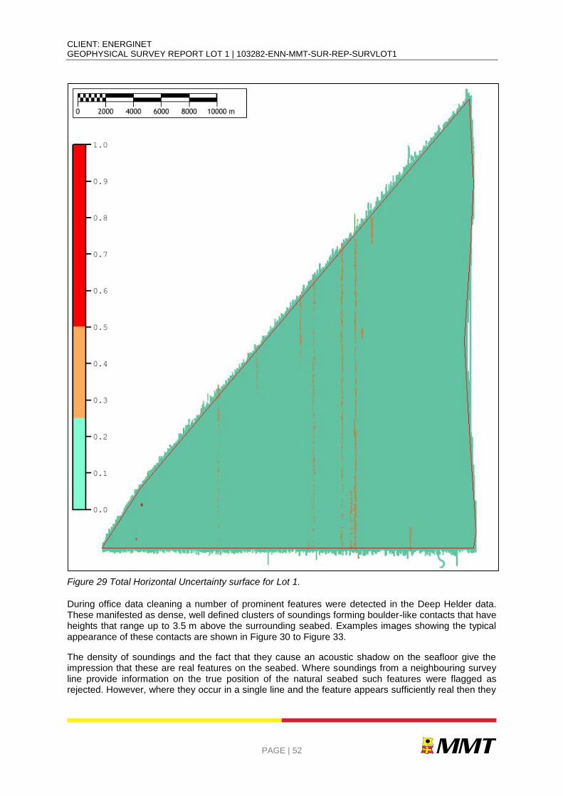
CLIENT: ENERGINET GEOPHYSICAL SURVEY REPORT LOT 1 | 103282-ENN-MMT-SUR-REP-SURVLOT1
PAGE | 52
Figure 29 Total Horizontal Uncertainty surface for Lot 1.
During office data cleaning a number of prominent features were detected in the Deep Helder data. These manifested as dense, well defined clusters of soundings forming boulder-like contacts that have heights that range up to 3.5 m above the surrounding seabed. Examples images showing the typical appearance of these contacts are shown in Figure 30 to Figure 33.
The density of soundings and the fact that they cause an acoustic shadow on the seafloor give the impression that these are real features on the seabed. Where soundings from a neighbouring survey line provide information on the true position of the natural seabed such features were flagged as rejected. However, where they occur in a single line and the feature appears sufficiently real then they

CLIENT: ENERGINET GEOPHYSICAL SURVEY REPORT LOT 1 | 103282-ENN-MMT-SUR-REP-SURVLOT1
PAGE | 53
have been retained. On balance it was considered better to include a prominent contact that could have implications for engineering operations. Such artefacts could be disproved by a future site-specific survey.
These prominent boulder-like features can be identified by areas with very high slope angles. Angles of up to 75° are observed around the features that remain in the dataset. In comparison slope angles around natural seabed features reach a maximum value of 43°. All such erroneous features have been identified and included as a separate feature in the GIS deliverables.
To find the locations of these anomalous features contours were generated at 10° intervals from the slope raster in ArcGIS. Since the features have high slope angles and cover small areas contours with lengths longer than 20 m and angles less than 10° were discarded. This method was assessed against known anomalous features in the ArcGIS rasters. The shapefile of the remaining contours was imported to Caris HIPS and the features highlighted were opened in the Subset Editor in order to determine whether it was an anomaly. Where it was confident the highlighted area was a natural seabed feature the contours were removed from the shapefile until only the MBES anomalies remained. At this point the lines were rationalised so that only a single contour was located over each MBES anomaly.
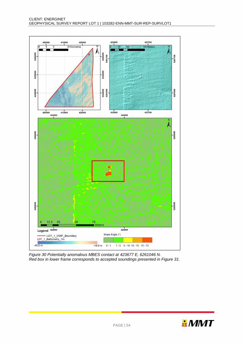
CLIENT: ENERGINET GEOPHYSICAL SURVEY REPORT LOT 1 | 103282-ENN-MMT-SUR-REP-SURVLOT1
PAGE | 54
Figure 30 Potentially anomalous MBES contact at 423677 E, 6261046 N. Red box in lower frame corresponds to accepted soundings presented in Figure 31.
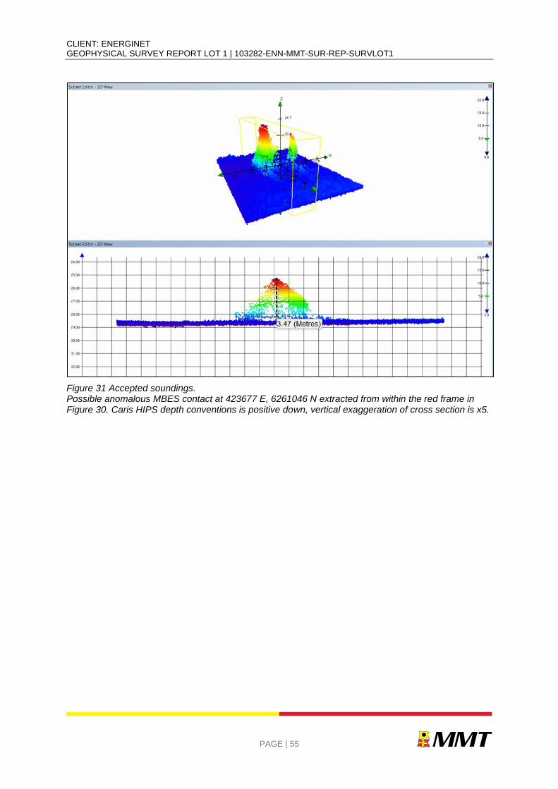
CLIENT: ENERGINET GEOPHYSICAL SURVEY REPORT LOT 1 | 103282-ENN-MMT-SUR-REP-SURVLOT1
PAGE | 55
Figure 31 Accepted soundings. Possible anomalous MBES contact at 423677 E, 6261046 N extracted from within the red frame in Figure 30. Caris HIPS depth conventions is positive down, vertical exaggeration of cross section is x5.
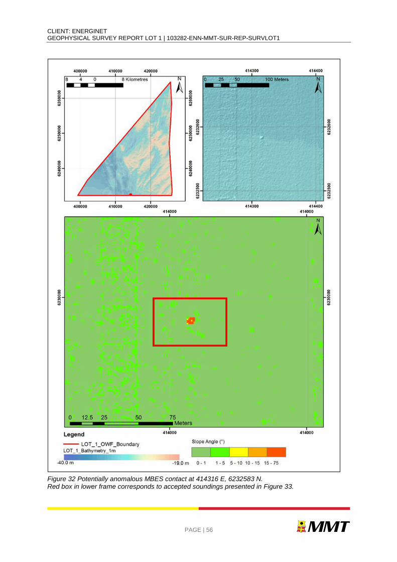
CLIENT: ENERGINET GEOPHYSICAL SURVEY REPORT LOT 1 | 103282-ENN-MMT-SUR-REP-SURVLOT1
PAGE | 56
Figure 32 Potentially anomalous MBES contact at 414316 E, 6232583 N. Red box in lower frame corresponds to accepted soundings presented in Figure 33.
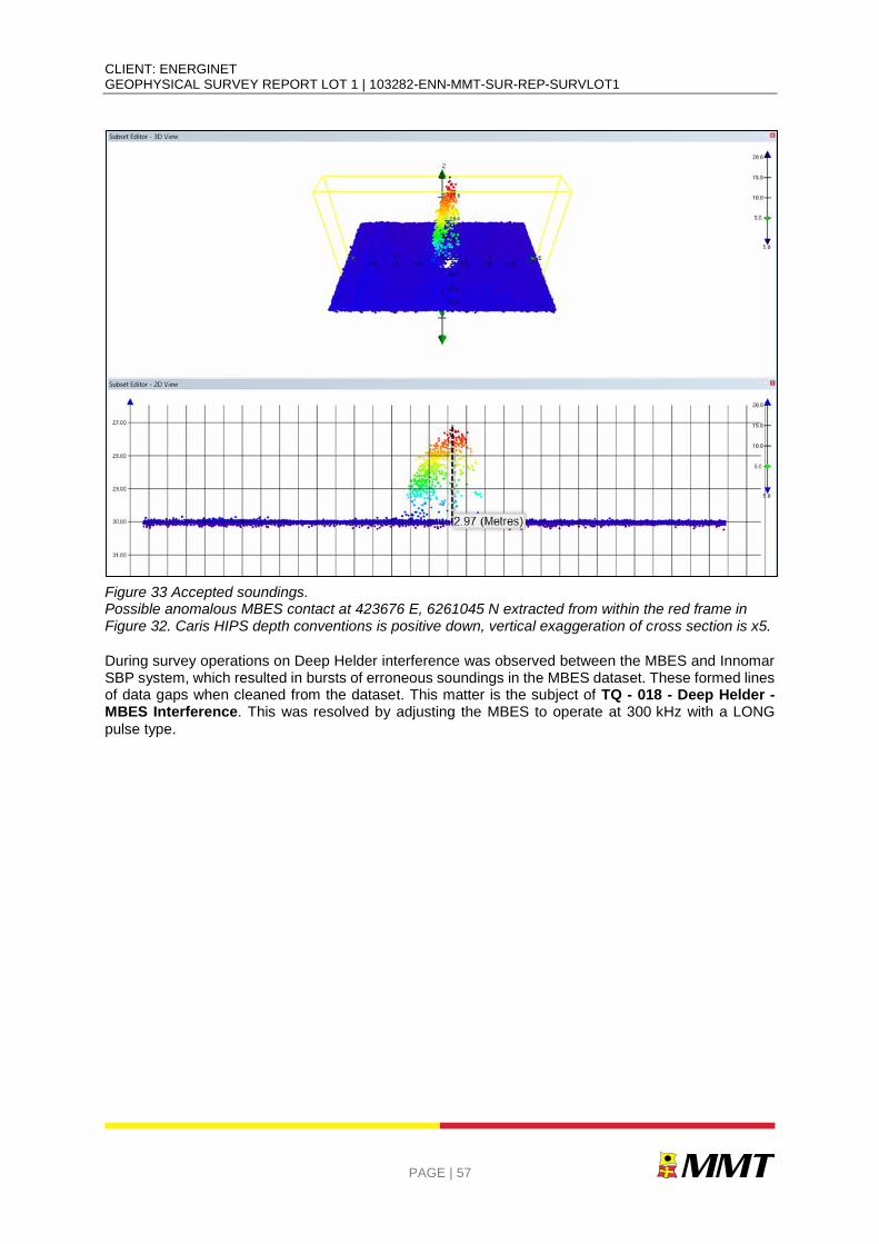
CLIENT: ENERGINET GEOPHYSICAL SURVEY REPORT LOT 1 | 103282-ENN-MMT-SUR-REP-SURVLOT1
PAGE | 57
Figure 33 Accepted soundings. Possible anomalous MBES contact at 423676 E, 6261045 N extracted from within the red frame in Figure 32. Caris HIPS depth conventions is positive down, vertical exaggeration of cross section is x5.
During survey operations on Deep Helder interference was observed between the MBES and Innomar SBP system, which resulted in bursts of erroneous soundings in the MBES dataset. These formed lines of data gaps when cleaned from the dataset. This matter is the subject of TQ - 018 - Deep Helder - MBES Interference. This was resolved by adjusting the MBES to operate at 300 kHz with a LONG
pulse type.

CLIENT: ENERGINET GEOPHYSICAL SURVEY REPORT LOT 1 | 103282-ENN-MMT-SUR-REP-SURVLOT1
PAGE | 58
5.2| BACKSCATTER DATA
To assess the quality of the final processed backscatter data the 8 bit GeoTiff rasters were exported from FMGT and combined to create an overview image for the entire Lot 1 survey (Figure 34). To ensure the individual block mosaics blended as homogeneously as possible the colour scales were adjusted prior to export so that each mosaic showed the same range of values. This minimised any artefact relating to the blending process, which was performed using FME. This step is necessary as it is not possible, due to software limitations, to process the entire survey area into a single mosaic at such a high resolution.
Assessment of the combined mosaic indicates that the boundaries between different sediment types were well delineated with good agreement between the relative intensities of the data acquired by Deep Helder and Franklin.
Some artefacts are present and mostly manifest as stripes aligned with the survey line direction. Both Deep Helder and Franklin were fitted with the same type of MBES system, a Kongsberg EM2040D, which should mitigate differences observed between the two datasets. However, differences in the placement of the sonars on each vessel could play a role in generating artefacts between the two datasets. These artefacts appear to be exacerbated during periods of poor weather and are most prominent for the Deep Helder data. Additionally, individual "beam busts" occur during instances of strong vessel motion or when air bubbles are drawn across the MBES transducers' face. These appear as short, dark lines that run perpendicular to the survey line direction.
Despite the presence of these artefacts, the backscatter data is of sufficient quality to derive sediment boundaries and assist in the identification of contacts such as boulders (Figure 35).
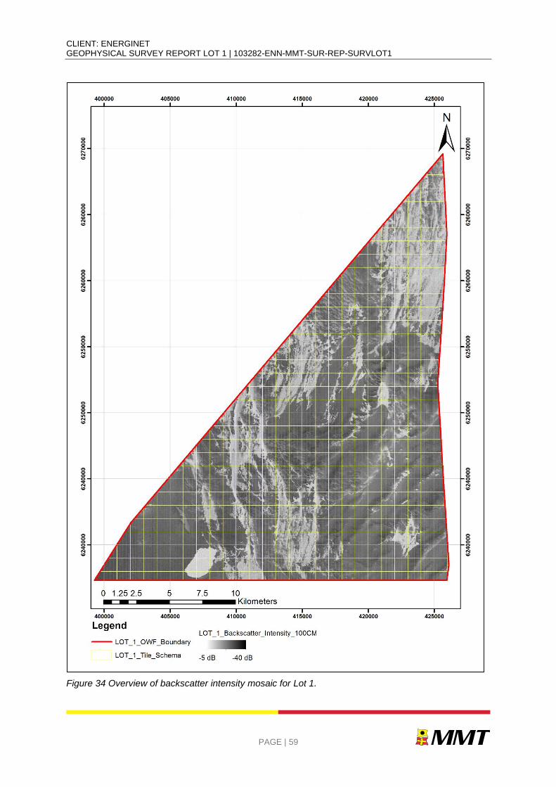
CLIENT: ENERGINET GEOPHYSICAL SURVEY REPORT LOT 1 | 103282-ENN-MMT-SUR-REP-SURVLOT1
PAGE | 59
Figure 34 Overview of backscatter intensity mosaic for Lot 1.
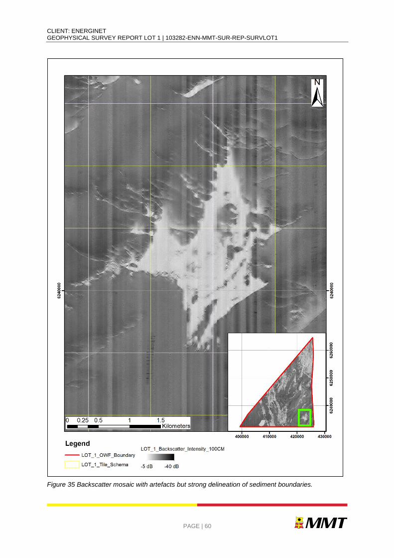
CLIENT: ENERGINET GEOPHYSICAL SURVEY REPORT LOT 1 | 103282-ENN-MMT-SUR-REP-SURVLOT1
PAGE | 60
Figure 35 Backscatter mosaic with artefacts but strong delineation of sediment boundaries.
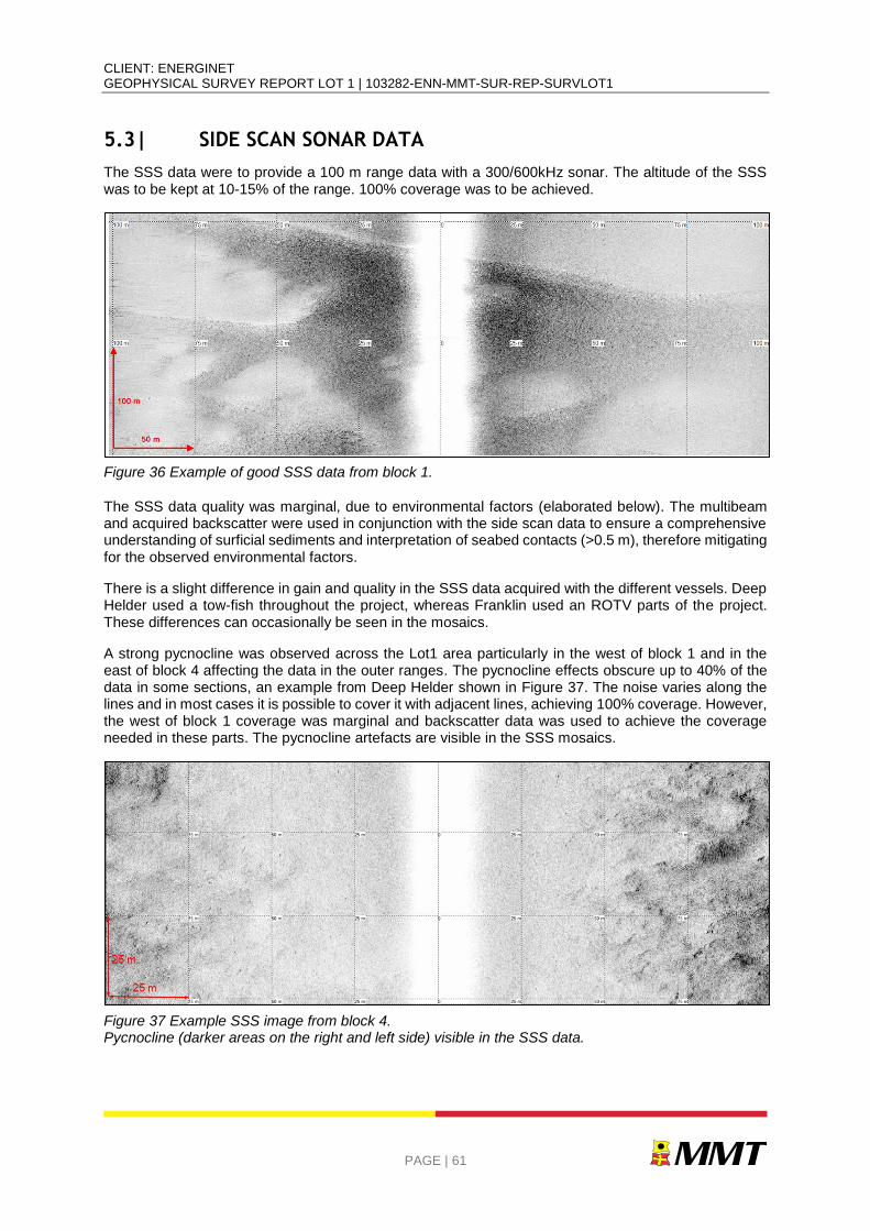
CLIENT: ENERGINET GEOPHYSICAL SURVEY REPORT LOT 1 | 103282-ENN-MMT-SUR-REP-SURVLOT1
PAGE | 61
5.3| SIDE SCAN SONAR DATA
The SSS data were to provide a 100 m range data with a 300/600kHz sonar. The altitude of the SSS was to be kept at 10-15% of the range. 100% coverage was to be achieved.
Figure 36 Example of good SSS data from block 1.
The SSS data quality was marginal, due to environmental factors (elaborated below). The multibeam and acquired backscatter were used in conjunction with the side scan data to ensure a comprehensive understanding of surficial sediments and interpretation of seabed contacts (>0.5 m), therefore mitigating for the observed environmental factors.
There is a slight difference in gain and quality in the SSS data acquired with the different vessels. Deep Helder used a tow-fish throughout the project, whereas Franklin used an ROTV parts of the project. These differences can occasionally be seen in the mosaics.
A strong pycnocline was observed across the Lot1 area particularly in the west of block 1 and in the east of block 4 affecting the data in the outer ranges. The pycnocline effects obscure up to 40% of the data in some sections, an example from Deep Helder shown in Figure 37. The noise varies along the lines and in most cases it is possible to cover it with adjacent lines, achieving 100% coverage. However, the west of block 1 coverage was marginal and backscatter data was used to achieve the coverage needed in these parts. The pycnocline artefacts are visible in the SSS mosaics.
Figure 37 Example SSS image from block 4. Pycnocline (darker areas on the right and left side) visible in the SSS data.
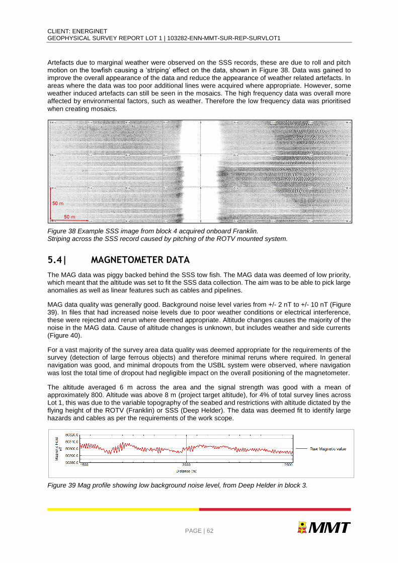
CLIENT: ENERGINET GEOPHYSICAL SURVEY REPORT LOT 1 | 103282-ENN-MMT-SUR-REP-SURVLOT1
PAGE | 62
Artefacts due to marginal weather were observed on the SSS records, these are due to roll and pitch motion on the towfish causing a ‘striping’ effect on the data, shown in Figure 38. Data was gained to improve the overall appearance of the data and reduce the appearance of weather related artefacts. In areas where the data was too poor additional lines were acquired where appropriate. However, some weather induced artefacts can still be seen in the mosaics. The high frequency data was overall more affected by environmental factors, such as weather. Therefore the low frequency data was prioritised when creating mosaics.
Figure 38 Example SSS image from block 4 acquired onboard Franklin. Striping across the SSS record caused by pitching of the ROTV mounted system.
5.4| MAGNETOMETER DATA
The MAG data was piggy backed behind the SSS tow fish. The MAG data was deemed of low priority, which meant that the altitude was set to fit the SSS data collection. The aim was to be able to pick large anomalies as well as linear features such as cables and pipelines.
MAG data quality was generally good. Background noise level varies from +/- 2 nT to +/- 10 nT (Figure 39). In files that had increased noise levels due to poor weather conditions or electrical interference, these were rejected and rerun where deemed appropriate. Altitude changes causes the majority of the noise in the MAG data. Cause of altitude changes is unknown, but includes weather and side currents (Figure 40).
For a vast majority of the survey area data quality was deemed appropriate for the requirements of the survey (detection of large ferrous objects) and therefore minimal reruns where required. In general navigation was good, and minimal dropouts from the USBL system were observed, where navigation was lost the total time of dropout had negligible impact on the overall positioning of the magnetometer.
The altitude averaged 6 m across the area and the signal strength was good with a mean of approximately 800. Altitude was above 8 m (project target altitude), for 4% of total survey lines across Lot 1, this was due to the variable topography of the seabed and restrictions with altitude dictated by the flying height of the ROTV (Franklin) or SSS (Deep Helder). The data was deemed fit to identify large hazards and cables as per the requirements of the work scope.
Figure 39 Mag profile showing low background noise level, from Deep Helder in block 3.
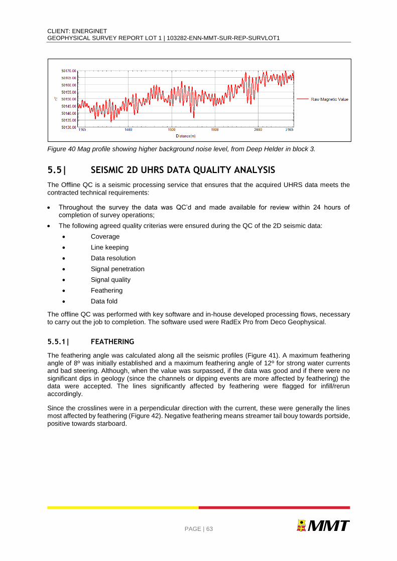
CLIENT: ENERGINET GEOPHYSICAL SURVEY REPORT LOT 1 | 103282-ENN-MMT-SUR-REP-SURVLOT1
PAGE | 63
Figure 40 Mag profile showing higher background noise level, from Deep Helder in block 3.
5.5| SEISMIC 2D UHRS DATA QUALITY ANALYSIS
The Offline QC is a seismic processing service that ensures that the acquired UHRS data meets the contracted technical requirements:
Throughout the survey the data was QC’d and made available for review within 24 hours of completion of survey operations;
The following agreed quality criterias were ensured during the QC of the 2D seismic data:
Coverage
Line keeping
Data resolution
Signal penetration
Signal quality
Feathering
Data fold
The offline QC was performed with key software and in-house developed processing flows, necessary to carry out the job to completion. The software used were RadEx Pro from Deco Geophysical.
5.5.1| FEATHERING
The feathering angle was calculated along all the seismic profiles (Figure 41). A maximum feathering angle of 8º was initially established and a maximum feathering angle of 12º for strong water currents and bad steering. Although, when the value was surpassed, if the data was good and if there were no significant dips in geology (since the channels or dipping events are more affected by feathering) the data were accepted. The lines significantly affected by feathering were flagged for infill/rerun accordingly.
Since the crosslines were in a perpendicular direction with the current, these were generally the lines most affected by feathering (Figure 42). Negative feathering means streamer tail bouy towards portside, positive towards starboard.
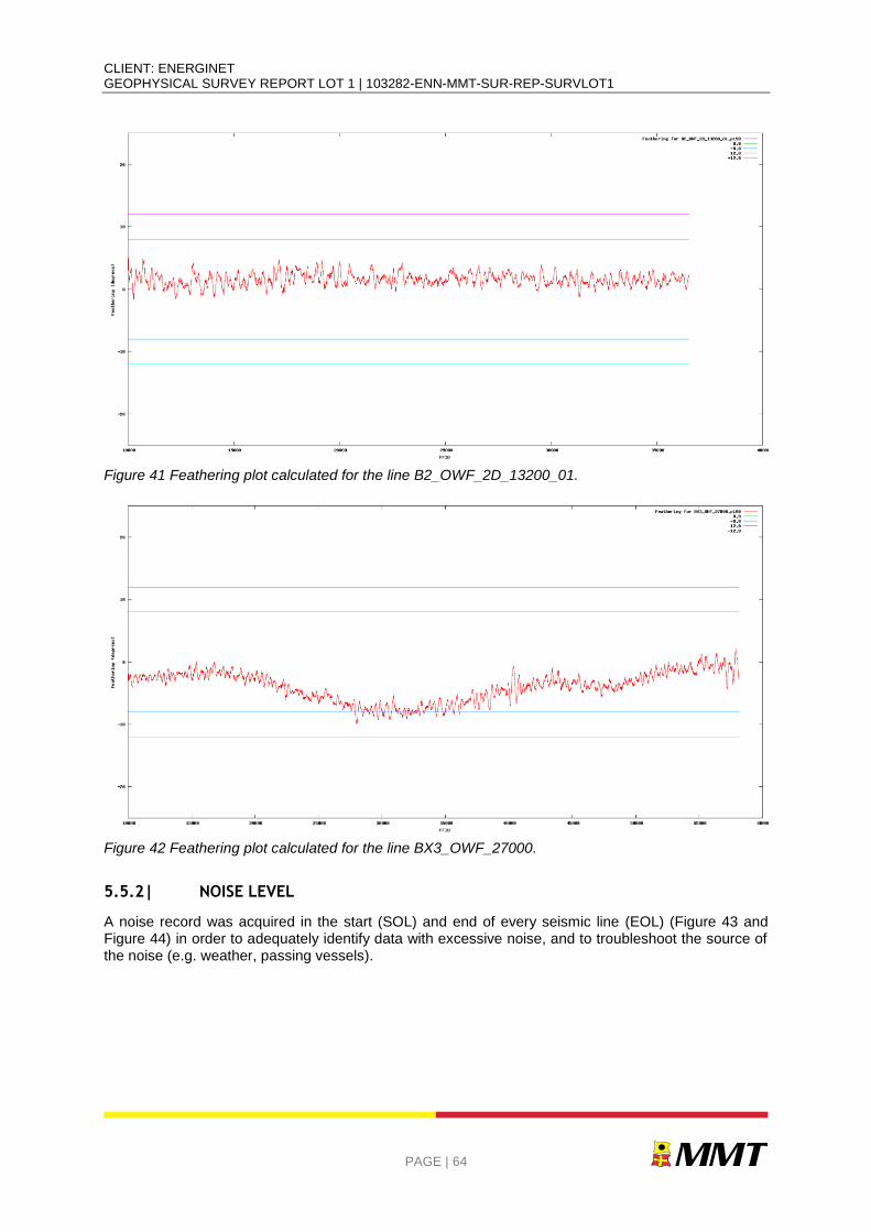
CLIENT: ENERGINET GEOPHYSICAL SURVEY REPORT LOT 1 | 103282-ENN-MMT-SUR-REP-SURVLOT1
PAGE | 64
Figure 41 Feathering plot calculated for the line B2_OWF_2D_13200_01.
Figure 42 Feathering plot calculated for the line BX3_OWF_27000.
5.5.2| NOISE LEVEL
A noise record was acquired in the start (SOL) and end of every seismic line (EOL) (Figure 43 and Figure 44) in order to adequately identify data with excessive noise, and to troubleshoot the source of the noise (e.g. weather, passing vessels).
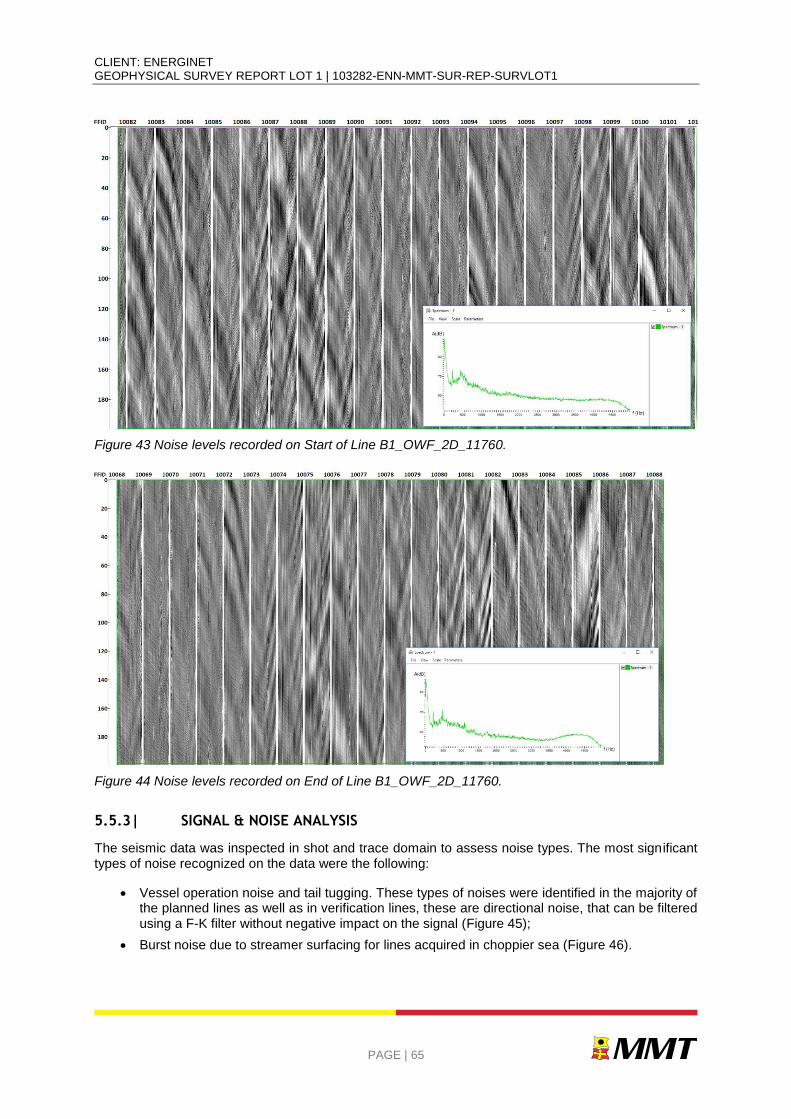
CLIENT: ENERGINET GEOPHYSICAL SURVEY REPORT LOT 1 | 103282-ENN-MMT-SUR-REP-SURVLOT1
PAGE | 65
Figure 43 Noise levels recorded on Start of Line B1_OWF_2D_11760.
Figure 44 Noise levels recorded on End of Line B1_OWF_2D_11760.
5.5.3| SIGNAL & NOISE ANALYSIS
The seismic data was inspected in shot and trace domain to assess noise types. The most significant types of noise recognized on the data were the following:
Vessel operation noise and tail tugging. These types of noises were identified in the majority of the planned lines as well as in verification lines, these are directional noise, that can be filtered using a F-K filter without negative impact on the signal (Figure 45);
Burst noise due to streamer surfacing for lines acquired in choppier sea (Figure 46).
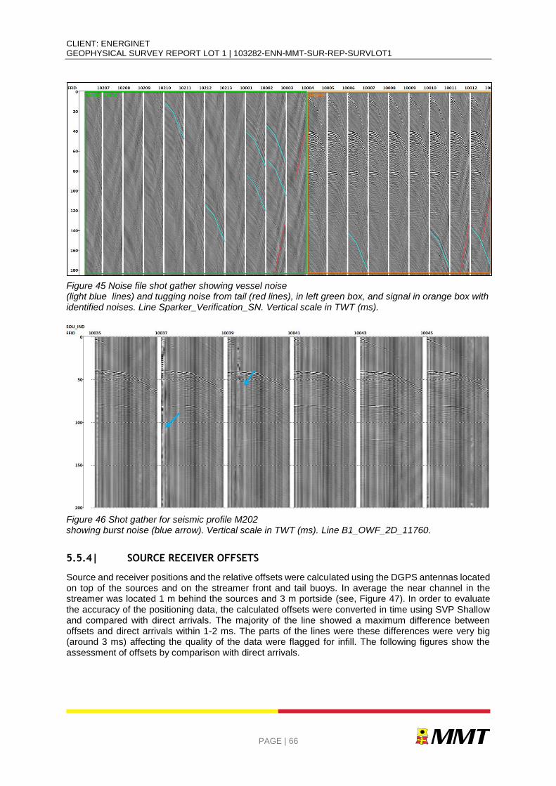
CLIENT: ENERGINET GEOPHYSICAL SURVEY REPORT LOT 1 | 103282-ENN-MMT-SUR-REP-SURVLOT1
PAGE | 66
Figure 45 Noise file shot gather showing vessel noise (light blue lines) and tugging noise from tail (red lines), in left green box, and signal in orange box with identified noises. Line Sparker_Verification_SN. Vertical scale in TWT (ms).
Figure 46 Shot gather for seismic profile M202 showing burst noise (blue arrow). Vertical scale in TWT (ms). Line B1_OWF_2D_11760.
5.5.4| SOURCE RECEIVER OFFSETS
Source and receiver positions and the relative offsets were calculated using the DGPS antennas located on top of the sources and on the streamer front and tail buoys. In average the near channel in the streamer was located 1 m behind the sources and 3 m portside (see, Figure 47). In order to evaluate the accuracy of the positioning data, the calculated offsets were converted in time using SVP Shallow and compared with direct arrivals. The majority of the line showed a maximum difference between offsets and direct arrivals within 1-2 ms. The parts of the lines were these differences were very big (around 3 ms) affecting the quality of the data were flagged for infill. The following figures show the assessment of offsets by comparison with direct arrivals.
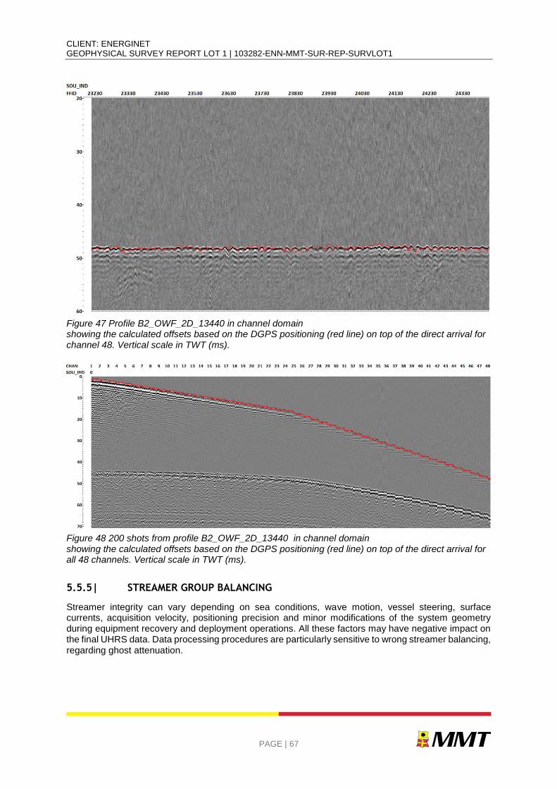
CLIENT: ENERGINET GEOPHYSICAL SURVEY REPORT LOT 1 | 103282-ENN-MMT-SUR-REP-SURVLOT1
PAGE | 67
Figure 47 Profile B2_OWF_2D_13440 in channel domain showing the calculated offsets based on the DGPS positioning (red line) on top of the direct arrival for channel 48. Vertical scale in TWT (ms).
Figure 48 200 shots from profile B2_OWF_2D_13440 in channel domain showing the calculated offsets based on the DGPS positioning (red line) on top of the direct arrival for all 48 channels. Vertical scale in TWT (ms).
5.5.5| STREAMER GROUP BALANCING
Streamer integrity can vary depending on sea conditions, wave motion, vessel steering, surface currents, acquisition velocity, positioning precision and minor modifications of the system geometry during equipment recovery and deployment operations. All these factors may have negative impact on the final UHRS data. Data processing procedures are particularly sensitive to wrong streamer balancing, regarding ghost attenuation.
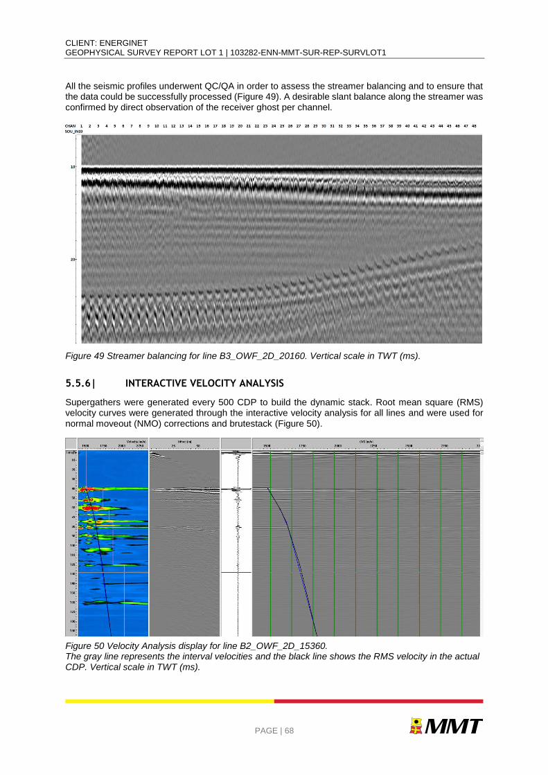
CLIENT: ENERGINET GEOPHYSICAL SURVEY REPORT LOT 1 | 103282-ENN-MMT-SUR-REP-SURVLOT1
PAGE | 68
All the seismic profiles underwent QC/QA in order to assess the streamer balancing and to ensure that the data could be successfully processed (Figure 49). A desirable slant balance along the streamer was confirmed by direct observation of the receiver ghost per channel.
Figure 49 Streamer balancing for line B3_OWF_2D_20160. Vertical scale in TWT (ms).
5.5.6| INTERACTIVE VELOCITY ANALYSIS
Supergathers were generated every 500 CDP to build the dynamic stack. Root mean square (RMS) velocity curves were generated through the interactive velocity analysis for all lines and were used for normal moveout (NMO) corrections and brutestack (Figure 50).
Figure 50 Velocity Analysis display for line B2_OWF_2D_15360. The gray line represents the interval velocities and the black line shows the RMS velocity in the actual CDP. Vertical scale in TWT (ms).
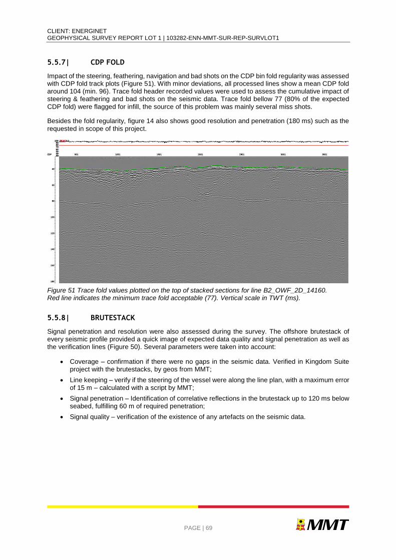
CLIENT: ENERGINET GEOPHYSICAL SURVEY REPORT LOT 1 | 103282-ENN-MMT-SUR-REP-SURVLOT1
PAGE | 69
5.5.7| CDP FOLD
Impact of the steering, feathering, navigation and bad shots on the CDP bin fold regularity was assessed with CDP fold track plots (Figure 51). With minor deviations, all processed lines show a mean CDP fold around 104 (min. 96). Trace fold header recorded values were used to assess the cumulative impact of steering & feathering and bad shots on the seismic data. Trace fold bellow 77 (80% of the expected CDP fold) were flagged for infill, the source of this problem was mainly several miss shots.
Besides the fold regularity, figure 14 also shows good resolution and penetration (180 ms) such as the requested in scope of this project.
Figure 51 Trace fold values plotted on the top of stacked sections for line B2_OWF_2D_14160. Red line indicates the minimum trace fold acceptable (77). Vertical scale in TWT (ms).
5.5.8| BRUTESTACK
Signal penetration and resolution were also assessed during the survey. The offshore brutestack of every seismic profile provided a quick image of expected data quality and signal penetration as well as the verification lines (Figure 50). Several parameters were taken into account:
Coverage – confirmation if there were no gaps in the seismic data. Verified in Kingdom Suite project with the brutestacks, by geos from MMT;
Line keeping – verify if the steering of the vessel were along the line plan, with a maximum error of 15 m – calculated with a script by MMT;
Signal penetration – Identification of correlative reflections in the brutestack up to 120 ms below seabed, fulfilling 60 m of required penetration;
Signal quality – verification of the existence of any artefacts on the seismic data.
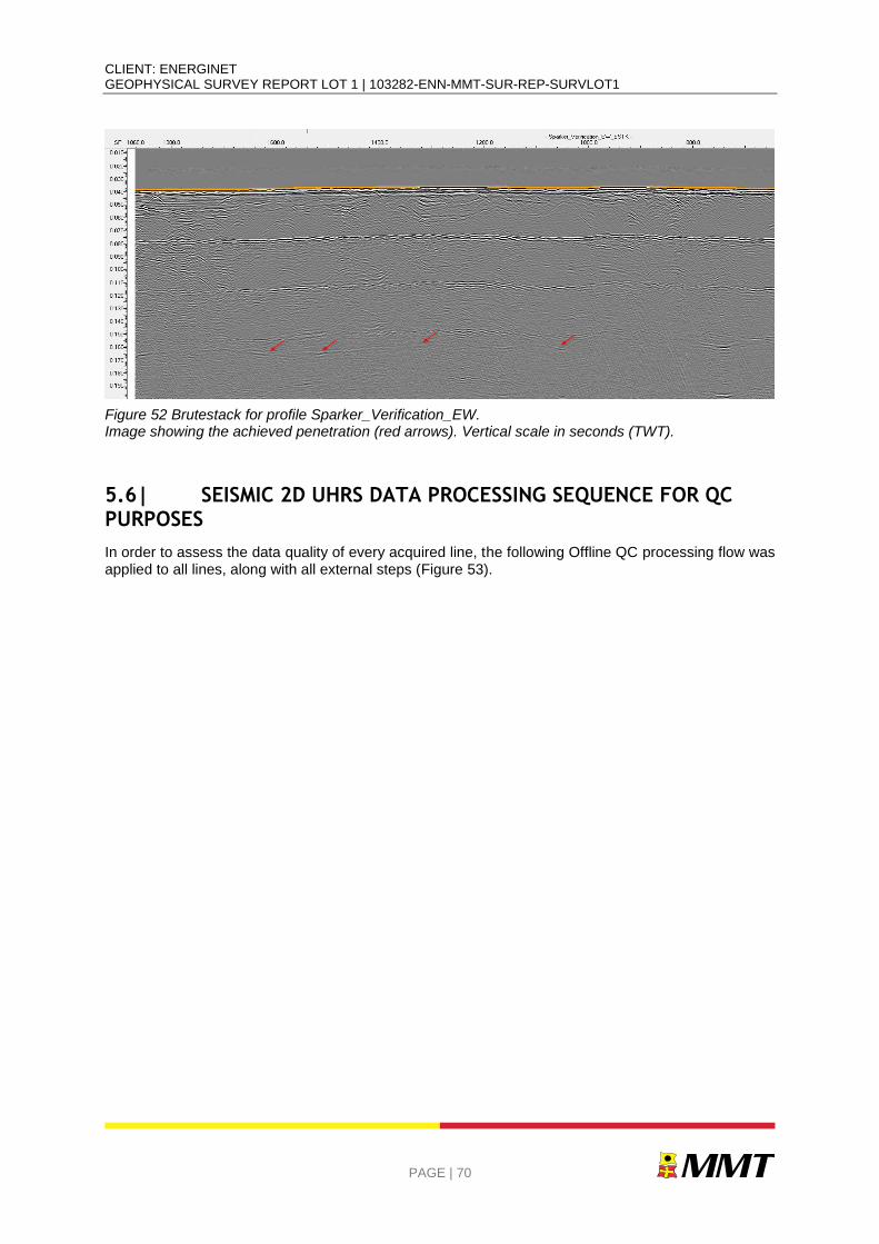
CLIENT: ENERGINET GEOPHYSICAL SURVEY REPORT LOT 1 | 103282-ENN-MMT-SUR-REP-SURVLOT1
PAGE | 70
Figure 52 Brutestack for profile Sparker_Verification_EW. Image showing the achieved penetration (red arrows). Vertical scale in seconds (TWT).
5.6| SEISMIC 2D UHRS DATA PROCESSING SEQUENCE FOR QC PURPOSES
In order to assess the data quality of every acquired line, the following Offline QC processing flow was applied to all lines, along with all external steps (Figure 53).
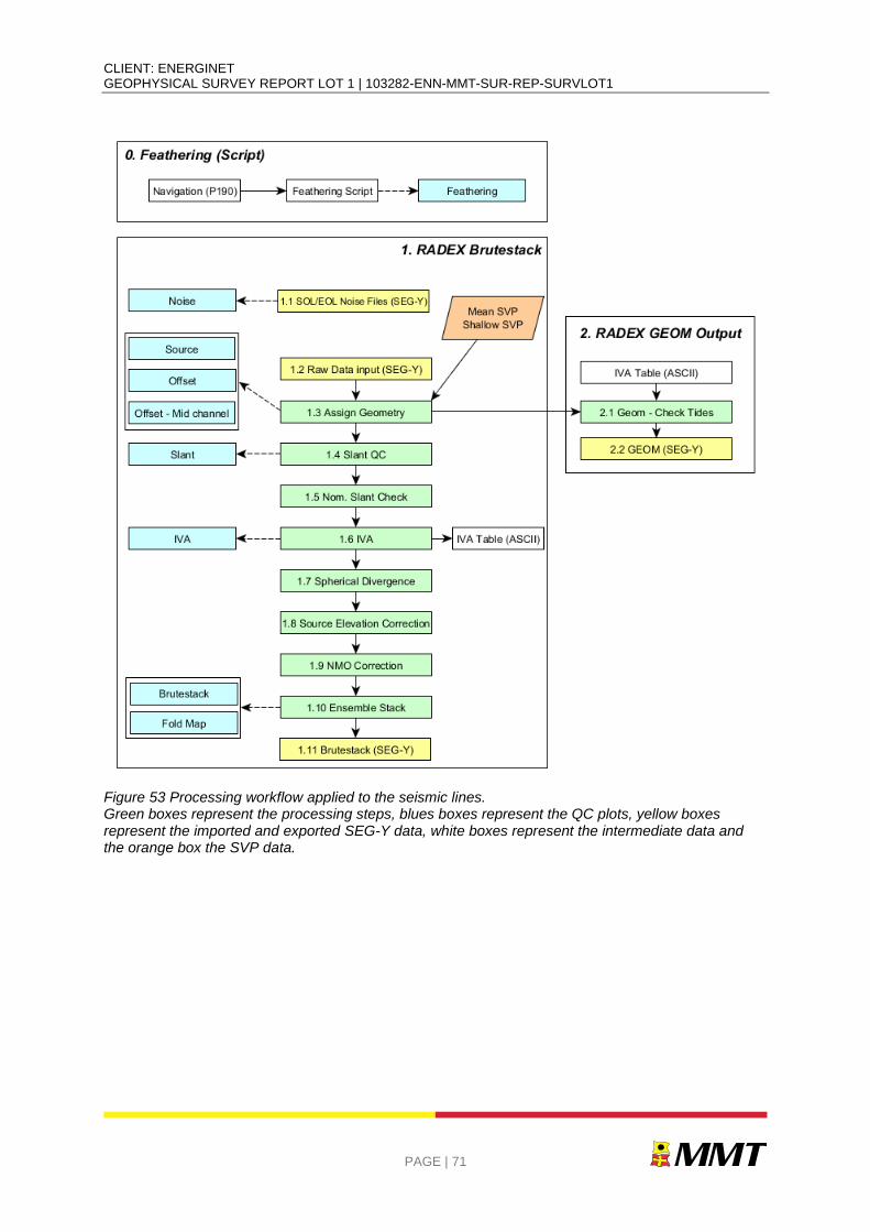
CLIENT: ENERGINET GEOPHYSICAL SURVEY REPORT LOT 1 | 103282-ENN-MMT-SUR-REP-SURVLOT1
PAGE | 71
Figure 53 Processing workflow applied to the seismic lines. Green boxes represent the processing steps, blues boxes represent the QC plots, yellow boxes represent the imported and exported SEG-Y data, white boxes represent the intermediate data and the orange box the SVP data.
CLIENT: ENERGINET GEOPHYSICAL SURVEY REPORT LOT 1 | 103282-ENN-MMT-SUR-REP-SURVLOT1
PAGE | 72
5.7| SEISMIC 2D UHRS DATA PROCESSING OFFICE
Quality control procedures were carried out throughout the processing scheme, as detailed within the present report and data control was registered along specifically designed logs. All processing steps were checked for the proper application of the seismic imaging enhancement. Several of these quality control plots were delivered to the client as part of this project submission, such as trace and offset QC; streamer slant check; source and receiver heave; image of the TRIM_STK (including trace fold); image of the FAST_MIG and image of final MIG (FULL).
Furthermore, at some stages, quality control supervision was carried out by the project’s Principal Interpreter to ensure that the seismic processing was being properly applied and for troubleshooting purposes. Finally, and after all intermediate quality controls, lines were inspected by both geophysicists and geologists for acceptance.
Several challenges were encountered during the processing stage of the 2D UHRS seismic dataset received, mainly related to the following:
Data quality on some profiles was negatively affected by sea conditions – mainly acoustic noise causing signal bursts and incoherent geometry along the affected lines;
Overall quality of the seismic deliverables was affected to different extents by the higher feathering angles, even though all processed lines were within specs regarding feathering values (feathering limits: 8 degrees due to steering and 12 degrees due to water currents).
Higher feathering may be also responsible for misties with the bathymetry;
Full signal penetration through the entire record length (200ms) achieved;
Seismic amplitude balancing was corrected in order for all seismic profiles to have a similar imaging of the subsurface;
Fine tuning of the post-stack migration in order to do not erase real geological features but also to remove undesired diffraction effects;
Artefacts related to the application of the velocity model (in the MIG datasets) or to the time-to-depth conversion (on the DPT datasets) were thoroughly checked for correction;
Overall, the contracted vertical seismic resolution was achieved - nominal target depth of 100m with a vertical resolution of 0.3m up to 40m BSB and 1 m for depths higher than 40m BSB. Seismic resolution improvement, both horizontal and vertical, was always a main concern in all processing steps.
A full processing report detailing all quality control steps, is available in Appendix D|.
5.8| SUB-BOTTOM PROFILER DATA – INNOMAR
The Innomar data were collected mainly to get a good resolution in the upper 10 m of the seabed. The settings of the Innomar were adjusted to achieve this.
SBP data quality was generally good (Figure 54). Some minor noise was introduced by the 2D UHRS sparker (Figure 55) on data acquired by Franklin, and some cavitation was observed on lines that were run in marginal weather on Deep Helder (Figure 55, Figure 56). Penetration achieved up to 10 m (target depth), this was variable across the site due to changing ground conditions; perceived penetration was dependent on the distribution of channelling beneath an initial coarse unit and dependent on the presence of observable units below Horizon 1 (Figure 54). Average penetration was 3-5 m.
There is a small difference perceived between data acquired on Franklin and Deep Helder, that can be observed on the curtain images of the data for both vessels. Deep Helder data shows a clearer image and seems to achieve better penetration than Franklin’s data. This could be related with the fact that each vessel had a different platform, and configuration of it could have been slightly different. However,
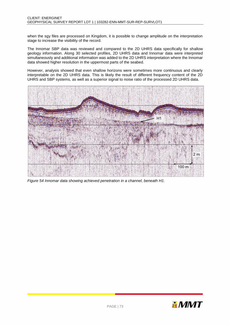
CLIENT: ENERGINET GEOPHYSICAL SURVEY REPORT LOT 1 | 103282-ENN-MMT-SUR-REP-SURVLOT1
PAGE | 73
when the sgy files are processed on Kingdom, it is possible to change amplitude on the interpretation stage to increase the visibility of the record.
The Innomar SBP data was reviewed and compared to the 2D UHRS data specifically for shallow geology information. Along 30 selected profiles, 2D UHRS data and Innomar data were interpreted simultaneously and additional information was added to the 2D UHRS interpretation where the Innomar data showed higher resolution in the uppermost parts of the seabed.
However, analysis showed that even shallow horizons were sometimes more continuous and clearly interpretable on the 2D UHRS data. This is likely the result of different frequency content of the 2D UHRS and SBP systems, as well as a superior signal to noise ratio of the processed 2D UHRS data.
Figure 54 Innomar data showing achieved penetration in a channel, beneath H1.
CLIENT: ENERGINET GEOPHYSICAL SURVEY REPORT LOT 1 | 103282-ENN-MMT-SUR-REP-SURVLOT1
PAGE | 74
Figure 55 Innomar data showing a minor data gap of approximately 2 m due to marginal weather and crosstalk from the sparker source.
Figure 56 Innomar data showing an instance of bubble rush from the vessel hull pitching in waves due to marginal weather.
CLIENT: ENERGINET GEOPHYSICAL SURVEY REPORT LOT 1 | 103282-ENN-MMT-SUR-REP-SURVLOT1
PAGE | 75
6| BACKGROUND DATA AND CLASSIFICATIONS
Client provided background information, GIS database and Arcadis desktop studies were the main resources used during data interpretation. Additionally, academic literature resources were used to support interpretations and are listed within the references in Section 10|.
6.1| SEABED GRADIENT CLASSIFICATION
The seabed gradient is classified according to Table 18.
Table 18 Seabed gradient classification.
CLASSIFICATION GRADIENT
Very Gentle < 1°
Gentle 1° - 4.9 °
Moderate 5° - 9.9°
Steep 10° - 14.9°
Very Steep > 15°
6.2| SEABED SEDIMENT CLASSIFICATION
The interpretation of surficial sediment types was derived from the acoustic character of the low frequency side scan sonar (SSS) data, and the interpretations aided by multibeam echo sounder (MBES) bathymetric 3D surfaces, multibeam backscatter (MBBS) and sub-bottom profiler (SBP) data, along with the results from the geotechnical campaign. During the review of the SSS survey data, higher intensity sonar returns (darker grey to black colours) were interpreted as relatively coarser grained sediments, and lower intensity sonar returns (lighter grey colours) were interpreted as relatively finer grained sediments. Bathymetric data was used to assist in boulder field interpretation and to correct for the effects of seabed slope on sonar returns
The ID column in Table 19 defines the colour in the charts for the specific sediment type. All particle sizes refer to the soil classification in ISO 14688-1 (2002).
CLIENT: ENERGINET GEOPHYSICAL SURVEY REPORT LOT 1 | 103282-ENN-MMT-SUR-REP-SURVLOT1
PAGE | 76
Table 19 Sediment classification.
ID SSS Image BS Image Acoustic Description Lithological Interpretation
Low acoustic reflectivity. No texture. Texture indicates wave and stream working of the sediment.
SILT
Predominantly silt, may contain clay and/or sand.
Medium acoustic reflectivity, slightly grainy texture.
SAND
Predominantly sand, may have minor fractions of clay, silt and/or gravel.
Medium to high acoustic reflectivity. Slightly grainy to grainy texture, coarse texture in places.
Gravelly SAND to sandy GRAVEL
Predominantly gravelly sand, may contain silt. The ratio between sand and gravel can vary within this sediment type.
High acoustic reflectivity. Grain, coarse texture.
GRAVEL
Predominantly gravel. May contain minor fractions of silt or clay. Ranges from slightly to very sandy. May also contain gravel sized shell fragments. May include cobbles.
Low to high acoustic reflectivity. Bands of high reflectivity interspersed with pockets of low reflectivity. Occasional grainy texture.
DIAMICTON
Predominantly gravelly sand. Constituents range between clay and boulders.
CLIENT: ENERGINET GEOPHYSICAL SURVEY REPORT LOT 1 | 103282-ENN-MMT-SUR-REP-SURVLOT1
PAGE | 77
6.3| SEABED FEATURE/BEDFORM CLASSIFICATION
The ID column in Table 20 defines the pattern in the charts for the specific feature type. Apart from the ones presented here, areas of trawl marks, as well as individual trawl marks were also digitized.
SSS, MBES and MBBS data have been used for interpretation of the seabed feature boundaries.
Table 20 Seabed features classification.
ID SSS Image BS Image Seabed Feature Criteria
Ripples
Wave length <5 m Height <1.0 m The wave length is the primary classifier.
Megaripples
Wave length <5 m – 25 m Height 0.5-1.5 m The wave length is the primary classifier.
Sand Waves
Wave length >25 m Height 1.5 – 25 m The wave length is the primary classifier.
Boulder Field Occasional boulders All >0.5 m
>10 and <20 boulders per 50x50 m.
Boulder Field Numerous boulders All >0.5 m
>20 boulders per 50x50 m.
CLIENT: ENERGINET GEOPHYSICAL SURVEY REPORT LOT 1 | 103282-ENN-MMT-SUR-REP-SURVLOT1
PAGE | 78
ID SSS Image BS Image Seabed Feature Criteria
Area of depressions
Occurs in SAND and gravelly SAND to sandy GRAVEL. Is seen as distinct depressions scattered across the seabed. No detection of gas in underlying sediments indicates the likely cause to be changes in seabed current regime rather than shallow biogenic gas
Mass Transport Deposits
Large areas of sediment movements in slope areas , appears in SAND and Gravelly SAND to sandy GRAVEL and in conjugation with sand waves.
The SSS and MBES contacts were classified according to the following criteria:
Boulder
Man-made object (MMO) (Debris, fishing gear, man-made structures etc.)
Wreck
Other
Boulders were grouped into boulder fields based on their spatial density:
- Occasional boulder field: >10 and <20 boulders per 50x50 m
- Numerous boulder field: > 20 boulders per 50x50 m
Boulders were not interpreted within boulder fields or within areas of diamicton.
When contacts were observed on the SSS and MBES they were included in the SSS contact list, and when contacts were only observed in the MBES they were included in the MBES contact list.
In the GIS database all MAG anomalies are categorized as MMO, due to the inherent uncertainties of magnetic anomaly interpretation.
In the combined contact listings, the MAG contacts were classified as
MMO (includes all anomalies that correlate to SSS or MBES contact, linear contacts and wrecks)
Discrete Anomaly (includes all anomalies with no further comment)
Geology (includes all anomalies that is inferred to be of a geological nature)
All MAG anomalies were compared to all MBES and SSS contacts. If a MAG anomaly was within 5 m of any contact detected in either MBES or SSS, it was deemed a correlation. A note was then made in the combined contact listing, as well as in the GIS database.
Anomalies forming a linear pattern were commented as such and these could indicate the presence of fishing gear, cables, wire/chain or anything of a ferrous linear nature. Some anomalies were inferred to be of a geological nature and these were also commented as such.

CLIENT: ENERGINET GEOPHYSICAL SURVEY REPORT LOT 1 | 103282-ENN-MMT-SUR-REP-SURVLOT1
PAGE | 79
Discrete anomalies are all anomalies detected in the MAG data lacking any additional information to aid the interpretation.
SBP contacts are selected when diffraction hyperbolas are present and can be clearly related to a single object. No hyperbolas were deemed sufficiently defined to be attributed to contacts.
CLIENT: ENERGINET GEOPHYSICAL SURVEY REPORT LOT 1 | 103282-ENN-MMT-SUR-REP-SURVLOT1
PAGE | 80
6.4| SUB-SEABED GEOLOGY CLASSIFICATION
The subsurface geology interpretation and description is based on the 2D UHRS and Innomar SBP assessment.
The original contract regarding the geomodel for this project was based on mapping six horizons, however eight horizons were mapped in order to properly capture the subsurface complexity of the geological framework in this site.
The mapped horizons correspond to the base of the seismic units of geological significance, exception to be made on one horizon (the deepest one which delineates a top). Two more horizons (seabed and processing last knee) were also incorporated into the stacking velocity model and depth-conversion model.
Seismic units were prefixed with ‘U’ (U10 to U50) and their base horizons with ‘H’ (H10 to H50), numbered accordingly and sequentially (from top to bottom). Deposits below H50 mapped horizon are included in the base seismic unit. The base seismic unit was divided into two sub units: SU98 and SU99 (T99 as a boundary between the two). For each seismic unit, a seismic profile is presented, displaying its main characteristics. All horizons that make up the Geomodel are to be included in the depth-conversion model, with the exception of T99.
Seismic reflectors were selected based on their geological and geotechnical significance and spatial continuity across the site. The individual horizons were picked using a combination of the physical characteristics of the seismic reflectors, seismic facies analysis and reflector terminations. The relevance of the horizons from a sequence stratigraphic standpoint was also a prime consideration.
The descriptions of the seismic units are provided according to the seismic facies, stratigraphic boundaries and internal reflector terminations. The units used are presented in Table 21.
Point source reflectors were not picked in the SBP or 2D UHRS data, since 3D seismic data is required to achieve reliable results.
For further information on the processing steps and classification methods, see Appendix D|.
CLIENT: ENERGINET GEOPHYSICAL SURVEY REPORT LOT 1 | 103282-ENN-MMT-SUR-REP-SURVLOT1
PAGE | 81
Table 21 Summary of the seismic units. S
EIS
MIC
UN
ITS
ACOUSTIC FACIES AND INTERNAL CONFIGURATION
LOWER BOUNDING
SURFACE
EX
PE
CT
ED
CO
MP
OS
ITIO
N
KIN
GD
OM
RE
FL
EC
TO
R
CO
LO
UR
STRATIGRAPHY (TENTATIVE CORRESPONDENCE)
MORPHOLOGY NATURE
U10
The seismic facies is (semi) transparent, it is also displays some faint internal layering. Some fossil sand waves are present
Wave cut ravinement
surface and is mostly flat
Erosive Clay to Sand,
organic material Light Green
Consists of marine sand deposits
Holocene
U20
Several types of seismic facies dominate this unit: (1) Relatively transparent facies with an internal erosive surface with high amplitude; (2) Laminated and sub-parallel reflections; (3) Acoustic (semi)transparency and very faint laminations; (4) Transparent and chaotic reflections. Internal erosional surfaces and truncated channel deposits are common
Irregular Erosive Clay to Sand,
organic material Cyan
Consists of infills of depressions and/or channels, which could be related to a lagoon system and partially a subaerial fluvial infill of a low stand erosive surface.
Early Holocene?
U30/U31
The Seismic facies shows chaotic reflections with variable amplitude. The internal reflectors’ are commonly poorly organized but locally may present some organization and layering
Irregular surface, relatively planar
Erosive Sand Brown
Strata distinctive negative acoustic impedance contrasts at its base. Could be correlated to a glaciolacustrine system.
Glacial period (Weichselian?)
U40 Displaying a range of seismic facies, base shows transparent and chaotic reflections. Channelization and an
irregular and undulated
Erosive Sand Spring green Likely associated with a glaciolacustrine or
Glacial period (Weichselian?)
CLIENT: ENERGINET GEOPHYSICAL SURVEY REPORT LOT 1 | 103282-ENN-MMT-SUR-REP-SURVLOT1
PAGE | 82
SE
ISM
IC U
NIT
S
ACOUSTIC FACIES AND INTERNAL CONFIGURATION
LOWER BOUNDING
SURFACE
EX
PE
CT
ED
CO
MP
OS
ITIO
N
KIN
GD
OM
RE
FL
EC
TO
R
CO
LO
UR
STRATIGRAPHY (TENTATIVE CORRESPONDENCE)
MORPHOLOGY NATURE
internal erosive surface. The upper part of this unit shows sub-parallel, wavy and continuous reflections with moderate amplitude. Shallow gas is
present
a similar relatively low-energy environment
U45
The Seismic facies are laminated dipping layers, downlaping onto the base horizon and sub-parallel facies with very irregular reflectors
Planar but contains localized
undulations Planar
Coarse Sediments
Violet
Could be related to a fluviodeltaic system in a moderate energy environment.
Interglacial period
(Eemian?)
U50 The seismic facies is well-organized, with (sub) parallel reflectors with good spatial continuity and fine layering
Irregular Carved channels Mostly muds, sands present towards the top
Light pink
Consists of fine layered sediments of glaciolacustrine origin and distinct laminated facies on the seismic profiles.
Elsterian and Saalian
glaciations?
Base seismic
Unit (SU98)
Subunit SU98 – the seismic facies are highly variable, mostly due to the intense tectonization and to the different sediments that composed this sub unit. Internal reflections appear typically wavy and folded, but can be chaotic, displaying complete incoherence
- - Clay to Sand -
The lowermost base unit, subdivided into SU98 and SU99, is a complex seismic unit comprising deformed sediments, which could be caused by glacial tectonics, valley infills and undeformed
Elsterian and Saalian
glaciations?
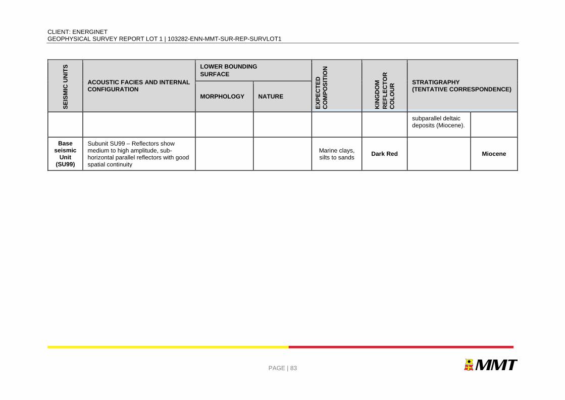
CLIENT: ENERGINET GEOPHYSICAL SURVEY REPORT LOT 1 | 103282-ENN-MMT-SUR-REP-SURVLOT1
PAGE | 83
SE
ISM
IC U
NIT
S
ACOUSTIC FACIES AND INTERNAL CONFIGURATION
LOWER BOUNDING
SURFACE
EX
PE
CT
ED
CO
MP
OS
ITIO
N
KIN
GD
OM
RE
FL
EC
TO
R
CO
LO
UR
STRATIGRAPHY (TENTATIVE CORRESPONDENCE)
MORPHOLOGY NATURE
subparallel deltaic deposits (Miocene).
Base seismic
Unit (SU99)
Subunit SU99 – Reflectors show medium to high amplitude, sub-horizontal parallel reflectors with good spatial continuity
Marine clays, silts to sands
Dark Red Miocene
CLIENT: ENERGINET GEOPHYSICAL SURVEY REPORT LOT 1 | 103282-ENN-MMT-SUR-REP-SURVLOT1
PAGE | 84
6.5| GEOTECHNICAL CLASSIFICATION
For details on the geotechnical classification, see Appendix C|.

CLIENT: ENERGINET GEOPHYSICAL SURVEY REPORT LOT 1 | 103282-ENN-MMT-SUR-REP-SURVLOT1
PAGE | 85
7| RESULTS
7.1| GENERAL
The results from the Lot 1 geophysical and geotechnical surveys are presented in this report together with associated north-up charts. The charts are presented in Appendix A|. The results of the geotechnical campaign is presented in Appendix C|.
To facilitate survey data management and survey planning, and to allow the fishing community to plan around the survey work, Lot 1 was divided into seven survey blocks. These included four blocks for the main lines (B1 to B4) and three blocks for the cross lines (X1 to X3), and are shown in Figure 5.
To assist with organisation in reporting, the survey area was separated into a tile schema. The layout of the tiles and the survey area are shown in Figure 57.
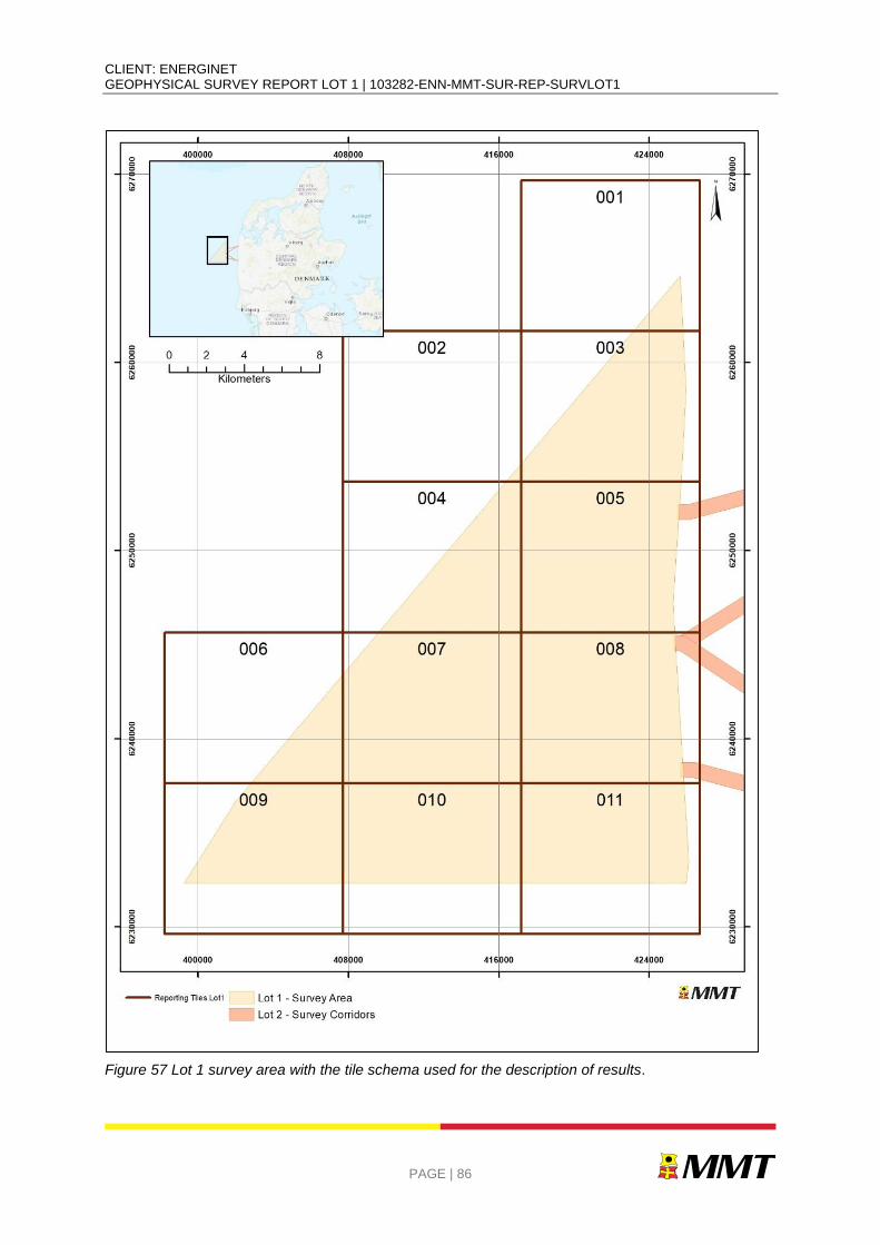
CLIENT: ENERGINET GEOPHYSICAL SURVEY REPORT LOT 1 | 103282-ENN-MMT-SUR-REP-SURVLOT1
PAGE | 86
Figure 57 Lot 1 survey area with the tile schema used for the description of results.

CLIENT: ENERGINET GEOPHYSICAL SURVEY REPORT LOT 1 | 103282-ENN-MMT-SUR-REP-SURVLOT1
PAGE | 87
7.2| BATHYMETRY
Overall the bathymetric depth changes moderately across Lot 1. The minimum surveyed depth is -20.38 m at 421 155 m E, 6248235 m N in the central part of the survey site (tile 005). The maximum depth surveyed depth is -35.4 m at 406 209 m E, 6 240 966 m N in the western area (tile 006). The depth range across the site is 15.0 m. Figure 58 shows an overview of the bathymetry within Lot 1.
Four profile lines are shown running from west to east across the site. These are derived from the following geophysical survey cross lines:
X1_OWF_8000 (northernmost)
X1_OWF_16000
X2_OWF_24000
X3_OWF_30000 (southernmost)
Profile data derived from these files is shown in Figure 59. The horizontal positions of the profiles have been shifted to match the KP values of the southernmost line, X3_OWF_30000. This has been done so the relative positions of the profiles are normalised and permits any features that may extend between the profiles to be visually aligned. The profiles have a strong vertical exaggeration so that features can be identified along the profiles.
The profiles generally show that the water depth generally increases from east to west across Lot 1 and highlights the varying range of depths observed especially towards the south of Lot 1.
The profiles are used to manage the presentation of the bathymetry results over the extensive Lot 1 survey area, with a sub-section of the report for each profile and regionally related features of interest.
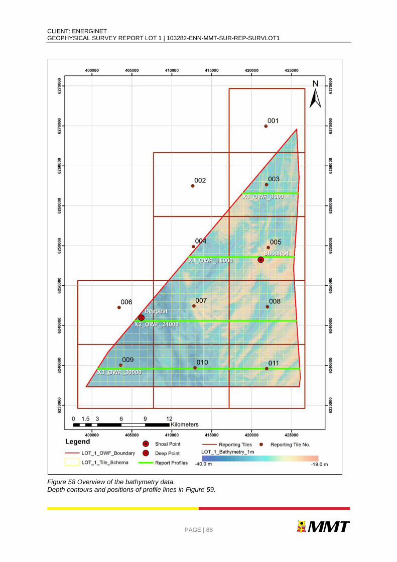
CLIENT: ENERGINET GEOPHYSICAL SURVEY REPORT LOT 1 | 103282-ENN-MMT-SUR-REP-SURVLOT1
PAGE | 88
Figure 58 Overview of the bathymetry data. Depth contours and positions of profile lines in Figure 59.
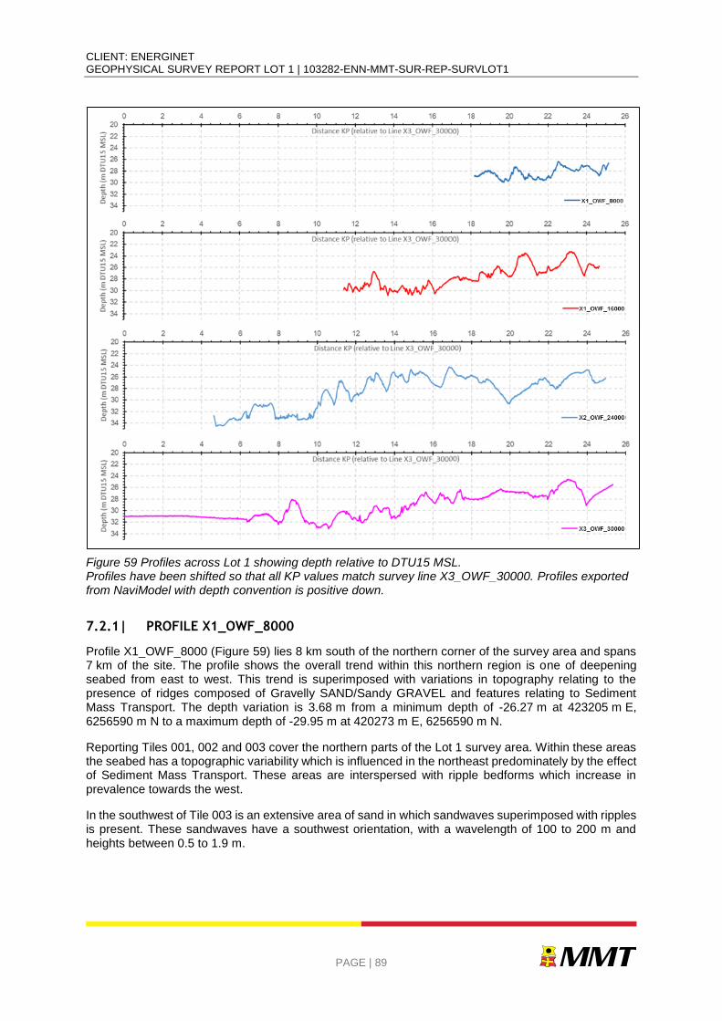
CLIENT: ENERGINET GEOPHYSICAL SURVEY REPORT LOT 1 | 103282-ENN-MMT-SUR-REP-SURVLOT1
PAGE | 89
Figure 59 Profiles across Lot 1 showing depth relative to DTU15 MSL. Profiles have been shifted so that all KP values match survey line X3_OWF_30000. Profiles exported from NaviModel with depth convention is positive down.
7.2.1| PROFILE X1_OWF_8000
Profile X1_OWF_8000 (Figure 59) lies 8 km south of the northern corner of the survey area and spans 7 km of the site. The profile shows the overall trend within this northern region is one of deepening seabed from east to west. This trend is superimposed with variations in topography relating to the presence of ridges composed of Gravelly SAND/Sandy GRAVEL and features relating to Sediment Mass Transport. The depth variation is 3.68 m from a minimum depth of -26.27 m at 423205 m E, 6256590 m N to a maximum depth of -29.95 m at 420273 m E, 6256590 m N.
Reporting Tiles 001, 002 and 003 cover the northern parts of the Lot 1 survey area. Within these areas the seabed has a topographic variability which is influenced in the northeast predominately by the effect of Sediment Mass Transport. These areas are interspersed with ripple bedforms which increase in prevalence towards the west.
In the southwest of Tile 003 is an extensive area of sand in which sandwaves superimposed with ripples is present. These sandwaves have a southwest orientation, with a wavelength of 100 to 200 m and heights between 0.5 to 1.9 m.
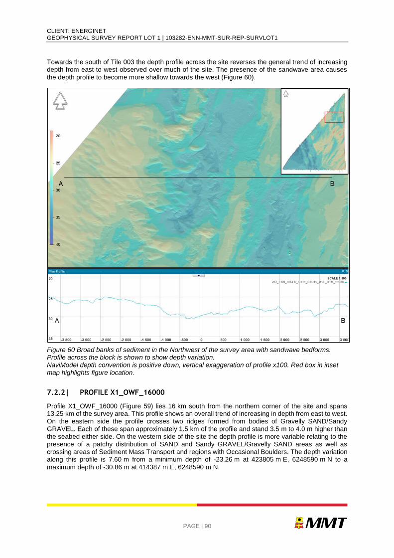
CLIENT: ENERGINET GEOPHYSICAL SURVEY REPORT LOT 1 | 103282-ENN-MMT-SUR-REP-SURVLOT1
PAGE | 90
Towards the south of Tile 003 the depth profile across the site reverses the general trend of increasing depth from east to west observed over much of the site. The presence of the sandwave area causes the depth profile to become more shallow towards the west (Figure 60).
Figure 60 Broad banks of sediment in the Northwest of the survey area with sandwave bedforms. Profile across the block is shown to show depth variation. NaviModel depth convention is positive down, vertical exaggeration of profile x100. Red box in inset map highlights figure location.
7.2.2| PROFILE X1_OWF_16000
Profile X1_OWF_16000 (Figure 59) lies 16 km south from the northern corner of the site and spans 13.25 km of the survey area. This profile shows an overall trend of increasing in depth from east to west. On the eastern side the profile crosses two ridges formed from bodies of Gravelly SAND/Sandy GRAVEL. Each of these span approximately 1.5 km of the profile and stand 3.5 m to 4.0 m higher than the seabed either side. On the western side of the site the depth profile is more variable relating to the presence of a patchy distribution of SAND and Sandy GRAVEL/Gravelly SAND areas as well as crossing areas of Sediment Mass Transport and regions with Occasional Boulders. The depth variation along this profile is 7.60 m from a minimum depth of -23.26 m at 423805 m E, 6248590 m N to a maximum depth of -30.86 m at 414387 m E, 6248590 m N.
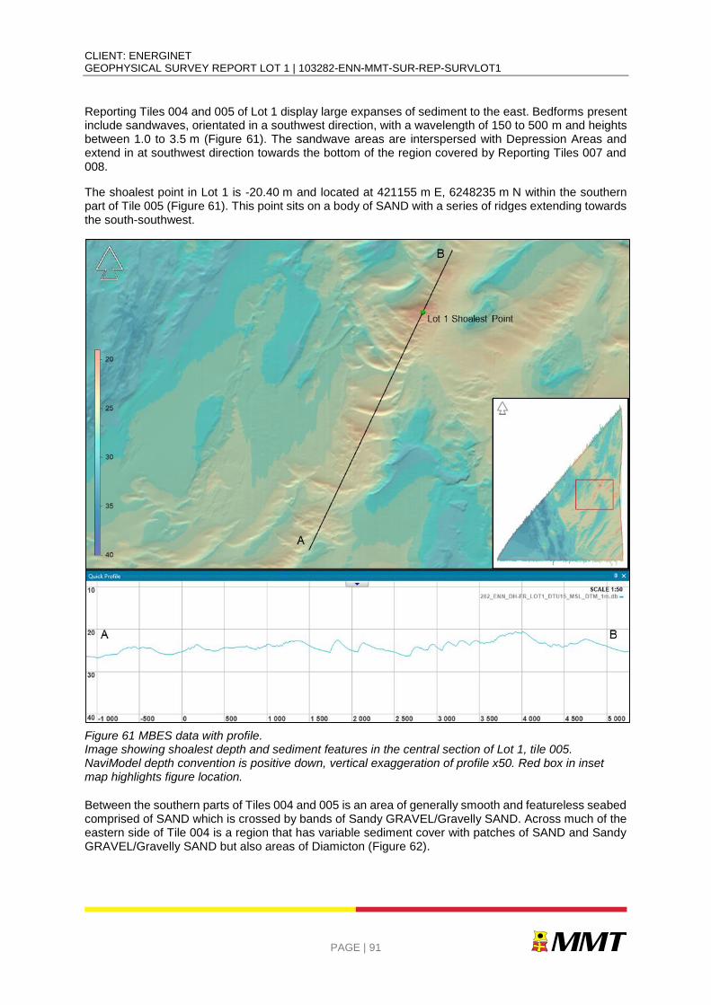
CLIENT: ENERGINET GEOPHYSICAL SURVEY REPORT LOT 1 | 103282-ENN-MMT-SUR-REP-SURVLOT1
PAGE | 91
Reporting Tiles 004 and 005 of Lot 1 display large expanses of sediment to the east. Bedforms present include sandwaves, orientated in a southwest direction, with a wavelength of 150 to 500 m and heights between 1.0 to 3.5 m (Figure 61). The sandwave areas are interspersed with Depression Areas and extend in at southwest direction towards the bottom of the region covered by Reporting Tiles 007 and 008.
The shoalest point in Lot 1 is -20.40 m and located at 421155 m E, 6248235 m N within the southern part of Tile 005 (Figure 61). This point sits on a body of SAND with a series of ridges extending towards the south-southwest.
Figure 61 MBES data with profile. Image showing shoalest depth and sediment features in the central section of Lot 1, tile 005. NaviModel depth convention is positive down, vertical exaggeration of profile x50. Red box in inset map highlights figure location.
Between the southern parts of Tiles 004 and 005 is an area of generally smooth and featureless seabed comprised of SAND which is crossed by bands of Sandy GRAVEL/Gravelly SAND. Across much of the eastern side of Tile 004 is a region that has variable sediment cover with patches of SAND and Sandy GRAVEL/Gravelly SAND but also areas of Diamicton (Figure 62).
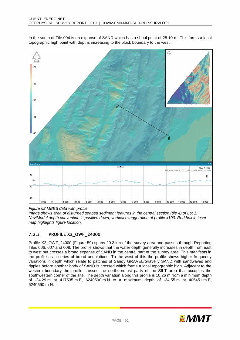
CLIENT: ENERGINET GEOPHYSICAL SURVEY REPORT LOT 1 | 103282-ENN-MMT-SUR-REP-SURVLOT1
PAGE | 92
In the south of Tile 004 is an expanse of SAND which has a shoal point of 25.10 m. This forms a local topographic high point with depths increasing to the block boundary to the west.
Figure 62 MBES data with profile. Image shows area of disturbed seabed sediment features in the central section (tile 4) of Lot 1. NaviModel depth convention is positive down, vertical exaggeration of profile x100. Red box in inset map highlights figure location.
7.2.3| PROFILE X2_OWF_24000
Profile X2_OWF_24000 (Figure 59) spans 20.3 km of the survey area and passes through Reporting Tiles 006, 007 and 008. The profile shows that the water depth generally increases in depth from east to west but crosses a broad expanse of SAND in the central part of the survey area. This manifests in the profile as a series of broad undulations. To the west of this the profile shows higher frequency variations in depth which relate to patches of Sandy GRAVEL/Gravelly SAND with sandwaves and ripples before another body of SAND is crossed which forms a local topographic high. Adjacent to the western boundary the profile crosses the northernmost parts of the SILT area that occupies the southwestern corner of the site. The depth variation along this profile is 10.26 m from a minimum depth of -24.29 m at 417535 m E, 6240590 m N to a maximum depth of -34.55 m at 405451 m E, 6240590 m N.
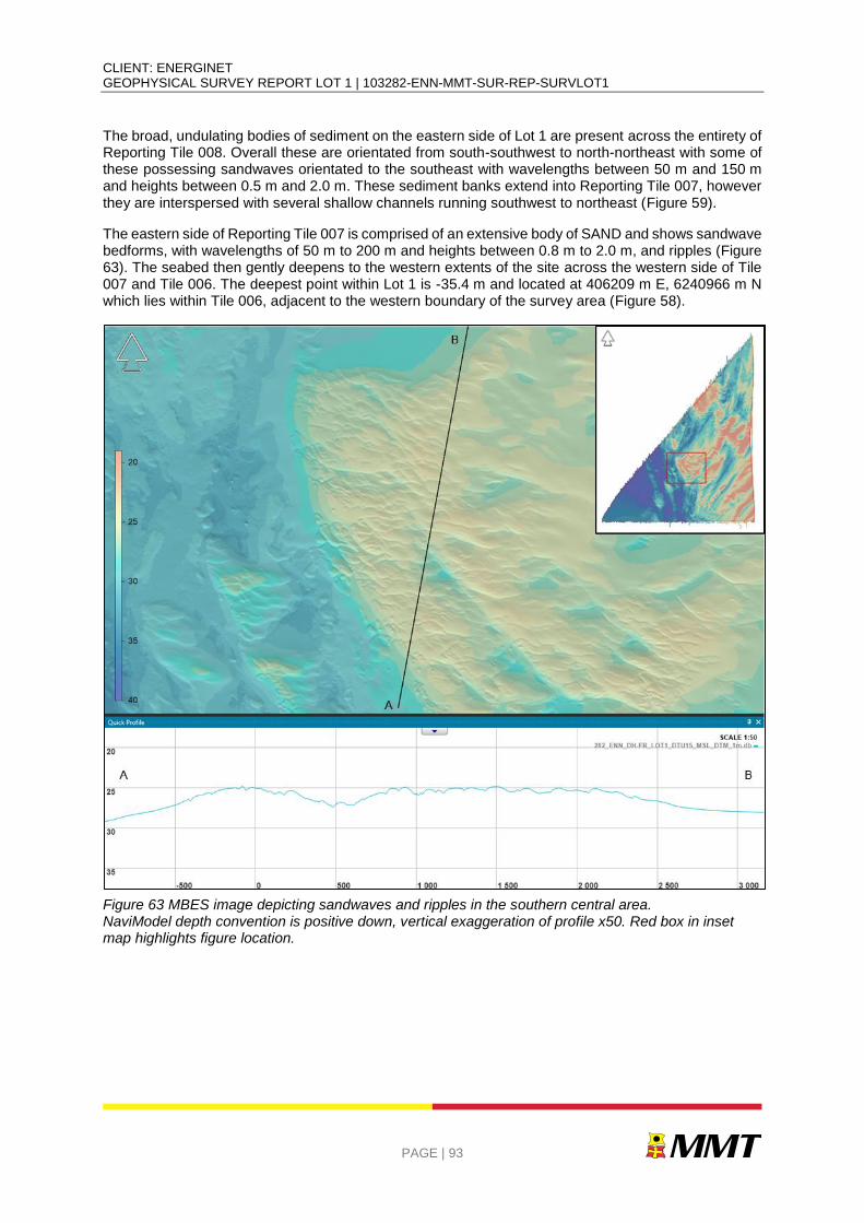
CLIENT: ENERGINET GEOPHYSICAL SURVEY REPORT LOT 1 | 103282-ENN-MMT-SUR-REP-SURVLOT1
PAGE | 93
The broad, undulating bodies of sediment on the eastern side of Lot 1 are present across the entirety of Reporting Tile 008. Overall these are orientated from south-southwest to north-northeast with some of these possessing sandwaves orientated to the southeast with wavelengths between 50 m and 150 m and heights between 0.5 m and 2.0 m. These sediment banks extend into Reporting Tile 007, however they are interspersed with several shallow channels running southwest to northeast (Figure 59).
The eastern side of Reporting Tile 007 is comprised of an extensive body of SAND and shows sandwave bedforms, with wavelengths of 50 m to 200 m and heights between 0.8 m to 2.0 m, and ripples (Figure 63). The seabed then gently deepens to the western extents of the site across the western side of Tile 007 and Tile 006. The deepest point within Lot 1 is -35.4 m and located at 406209 m E, 6240966 m N which lies within Tile 006, adjacent to the western boundary of the survey area (Figure 58).
Figure 63 MBES image depicting sandwaves and ripples in the southern central area. NaviModel depth convention is positive down, vertical exaggeration of profile x50. Red box in inset map highlights figure location.
CLIENT: ENERGINET GEOPHYSICAL SURVEY REPORT LOT 1 | 103282-ENN-MMT-SUR-REP-SURVLOT1
PAGE | 94
7.2.4| PROFILE X3_OWF_30000
Profile X3_OWF_30000 (Figure 59) spans 25.3 km of the survey area and passes through Reporting Tiles 009, 010 and 011. This profile reflects the overall trend of the site with depths generally increasing from east to west. This profile crosses numerous sediment bodies which form local topographic high points. This profile can be characterised in 3 generalised sections. The eastern third of the profile undulates gently as it crosses large bodies of SAND and Sandy Gravel/Gravelly SAND which display a south-southwest to north-north east orientation. The central third shows higher frequency variations in depth as the profile crosses patches of mixed sand and gravel sediments and areas of DIAMICTON and the western third is broadly smooth and flat and passes across an expansive region of SILT (Figure 64). The depth variation along this profile is 8.74 m from a minimum depth of -24.47 m at 423664 m E, 6234590 m N to a maximum depth of -33.21 m at 411276 m E, 6234590 m N.
Figure 64 MBES image with profile to show south to north seabed gradient in the southwest corner. NaviModel depth convention is positive down, vertical exaggeration of profile x100. Red box in inset map highlights figure location.
Reporting Tile 011 is dominated by the presence of the south-southwest to north-northeast orientated sediment bodies. These are generally wider and higher towards the eastern boundary and diminish in scale towards the western side of Tile 011. At the eastern side of Tile 010 the Sandy GRAVEL/Gravelly SAND areas become interspersed with ribbons of SAND and DIAMICTON. To the west of Tile 10 there
CLIENT: ENERGINET GEOPHYSICAL SURVEY REPORT LOT 1 | 103282-ENN-MMT-SUR-REP-SURVLOT1
PAGE | 95
are greater expanses of sediments including a large area of SAND to the north and DIAMICTION and SILT to the south. Generally though sediment distribution in this area is patchy and this causes greater topographic variability in the depth profiles (Figure 65).
Figure 65 MBES image with profile showing features in the central south area. NaviModel depth convention is positive down, vertical exaggeration of profile x100. Red box in inset map highlights figure location.

CLIENT: ENERGINET GEOPHYSICAL SURVEY REPORT LOT 1 | 103282-ENN-MMT-SUR-REP-SURVLOT1
PAGE | 96
7.2.5| SLOPE ANALYSIS
Slope angles were derived from the 1 m resolution bathymetry data in ArcGIS. This data has been used as the basis for examining gradients across the site as it less susceptible to picking up system noise as areas with high angles of slope.
The maximum slope around a feature, other than the boulder-like artefacts in the Deep Helder data, is 43° located in the far east of the survey area at 425434 m E, 6251748 m N. This corresponds to a large potential boulder contact (3.2 m (l) 3.1 m (w) 2.0 m (h)) that sits within a gently sloping depression at a general depth of -29 m. Scattered around this prominent feature are numerous smaller contacts. Although this feature is similar to those boulder-like contacts seen elsewhere in the Deep Helder data the feature was detected by Franklin and the local conditions provide confidence that this is a real object on the seabed. This feature is presented in Figure 66 and Figure 67.
CLIENT: ENERGINET GEOPHYSICAL SURVEY REPORT LOT 1 | 103282-ENN-MMT-SUR-REP-SURVLOT1
PAGE | 97
Figure 66 Possible boulder contact with 43° slope angle. Red box in lower frame corresponds to area of soundings shown in the following image.
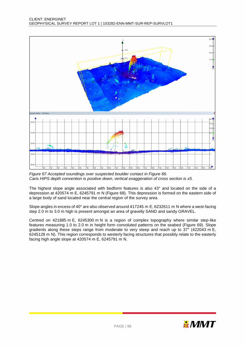
CLIENT: ENERGINET GEOPHYSICAL SURVEY REPORT LOT 1 | 103282-ENN-MMT-SUR-REP-SURVLOT1
PAGE | 98
Figure 67 Accepted soundings over suspected boulder contact in Figure 66. Caris HIPS depth convention is positive down, vertical exaggeration of cross section is x5.
The highest slope angle associated with bedform features is also 43° and located on the side of a depression at 420574 m E, 6245791 m N (Figure 68). This depression is formed on the eastern side of a large body of sand located near the central region of the survey area.
Slope angles in excess of 40° are also observed around 417245 m E, 6232611 m N where a west-facing step 2.0 m to 3.0 m high is present amongst an area of gravelly SAND and sandy GRAVEL.
Centred on 421885 m E, 6245300 m N is a region of complex topography where similar step-like features measuring 1.0 to 2.0 m in height form convoluted patterns on the seabed (Figure 69). Slope gradients along these steps range from moderate to very steep and reach up to 37° (422043 m E, 6245128 m N). This region corresponds to westerly facing structures that possibly relate to the easterly facing high angle slope at 420574 m E, 6245791 m N.
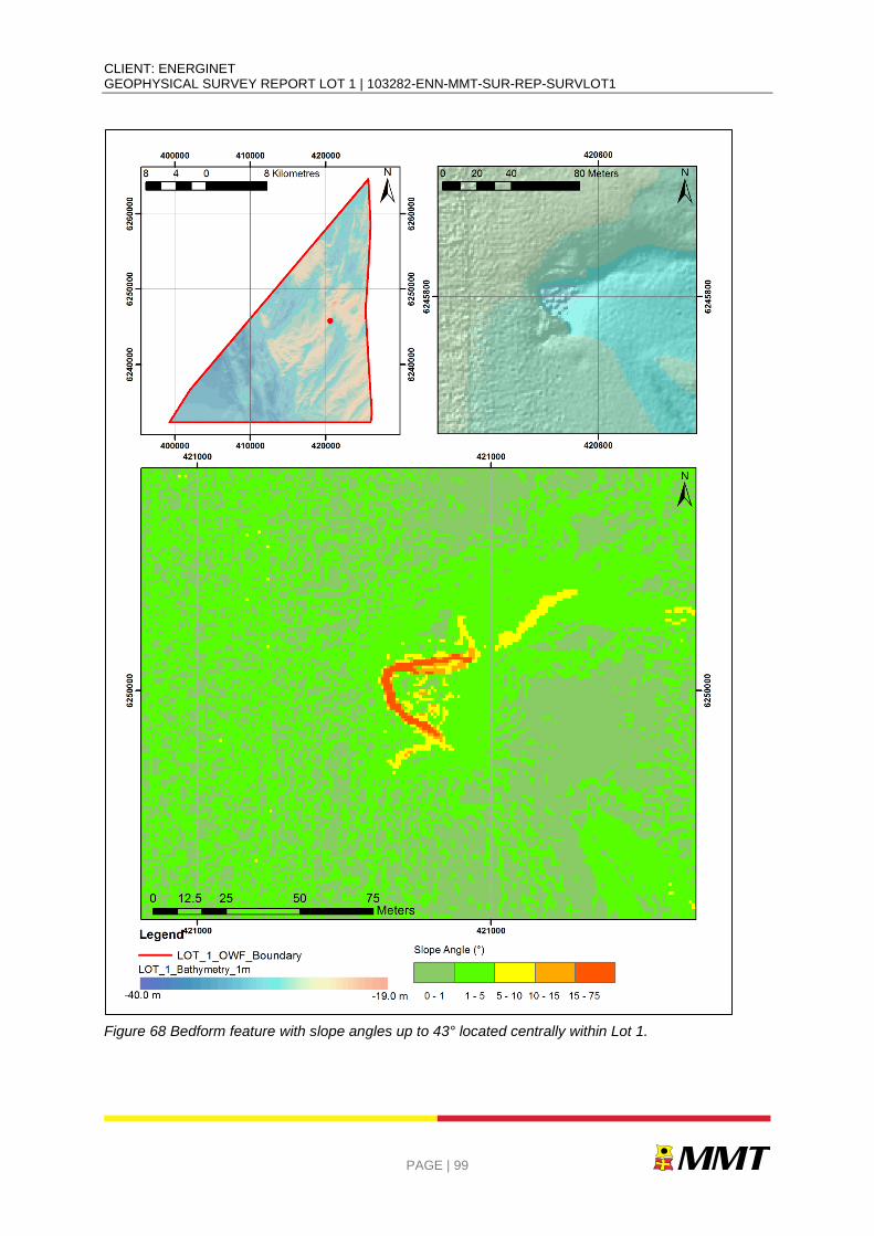
CLIENT: ENERGINET GEOPHYSICAL SURVEY REPORT LOT 1 | 103282-ENN-MMT-SUR-REP-SURVLOT1
PAGE | 99
Figure 68 Bedform feature with slope angles up to 43° located centrally within Lot 1.
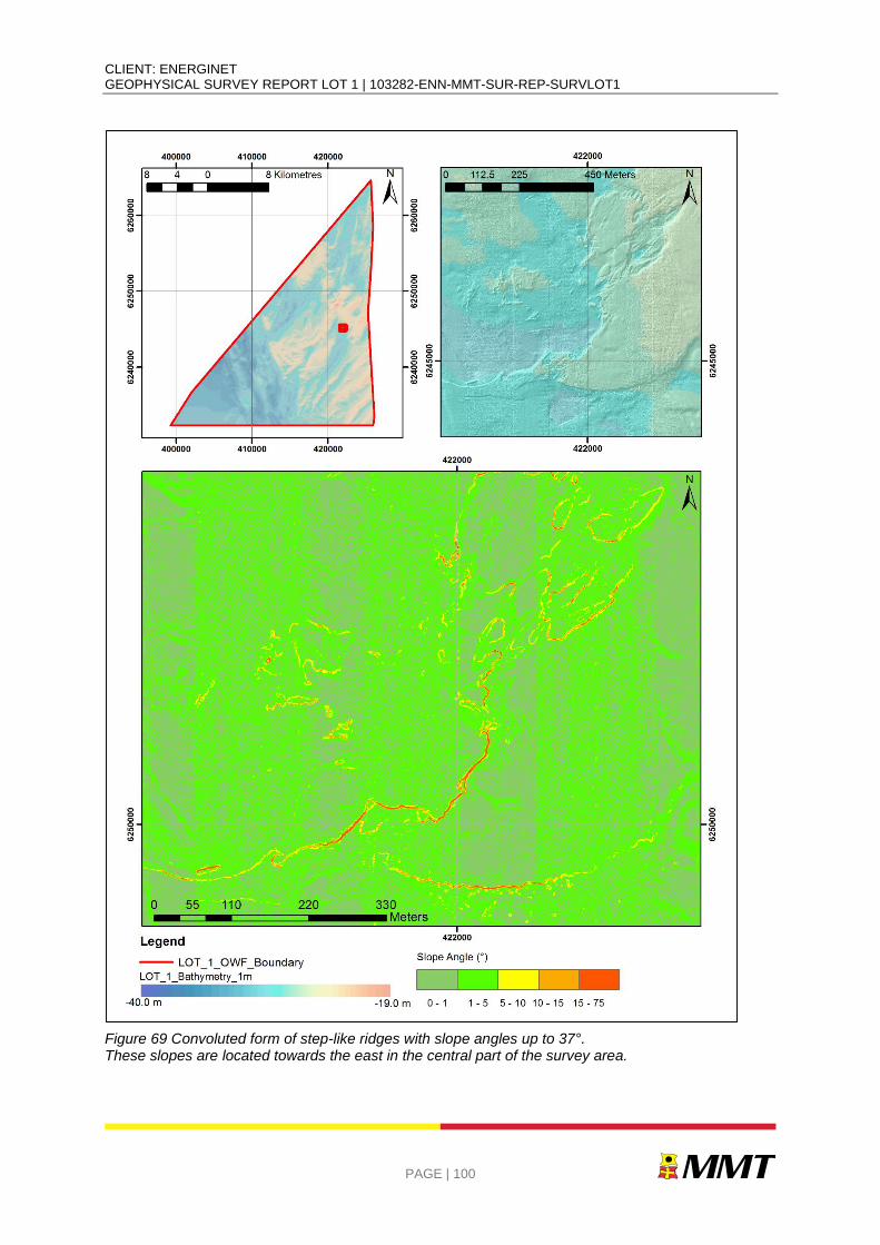
CLIENT: ENERGINET GEOPHYSICAL SURVEY REPORT LOT 1 | 103282-ENN-MMT-SUR-REP-SURVLOT1
PAGE | 100
Figure 69 Convoluted form of step-like ridges with slope angles up to 37°. These slopes are located towards the east in the central part of the survey area.

CLIENT: ENERGINET GEOPHYSICAL SURVEY REPORT LOT 1 | 103282-ENN-MMT-SUR-REP-SURVLOT1
PAGE | 101
More generally locations where slope angles are classed as very steep (>15°) are scattered widely across the survey area. Such high angles derived from the 1 m resolution bathymetry data are associated with larger contacts, such as boulders, but also the flanks of bodies of sediment, ridges and step-like features possibly associated with slumping and movement of sediments.
In addition to the features listed above, steep gradients (10° to 15°) highlight the irregular texture of diamicton due to the presence of numerous boulders. These regions are located in the northeast of the survey area and spanning the full height of the area just to the west of the centre of the survey area. Examples of such areas can be found at:
410303 m E, 6233403 m N
409933 m E, 6237734 m N
415157 m E, 6235084 m N
425222 m E, 6251680 m N.
Sand wave areas comprise approximately 78% of the Lot 1 survey area. Within these areas bedforms typically have a gently undulating topography. Slope angles are predominantly very gentle (<1°) and gentle (1° to 5°) with moderate angles (5° to 10°) highlighting the lee slopes of the most defined structures. Rare examples where angles are steep and very steep are restricted to the outer edges of sand wave fields where there is a change in sediment type (sand to Sandy GRAVEL/Gravelly SAND). This is shown in Figure 70 which shows the generally smooth nature of the topography with areas of yellow (moderate slope angles) visible at this scale highlighting the flanks of the bodies of sand.
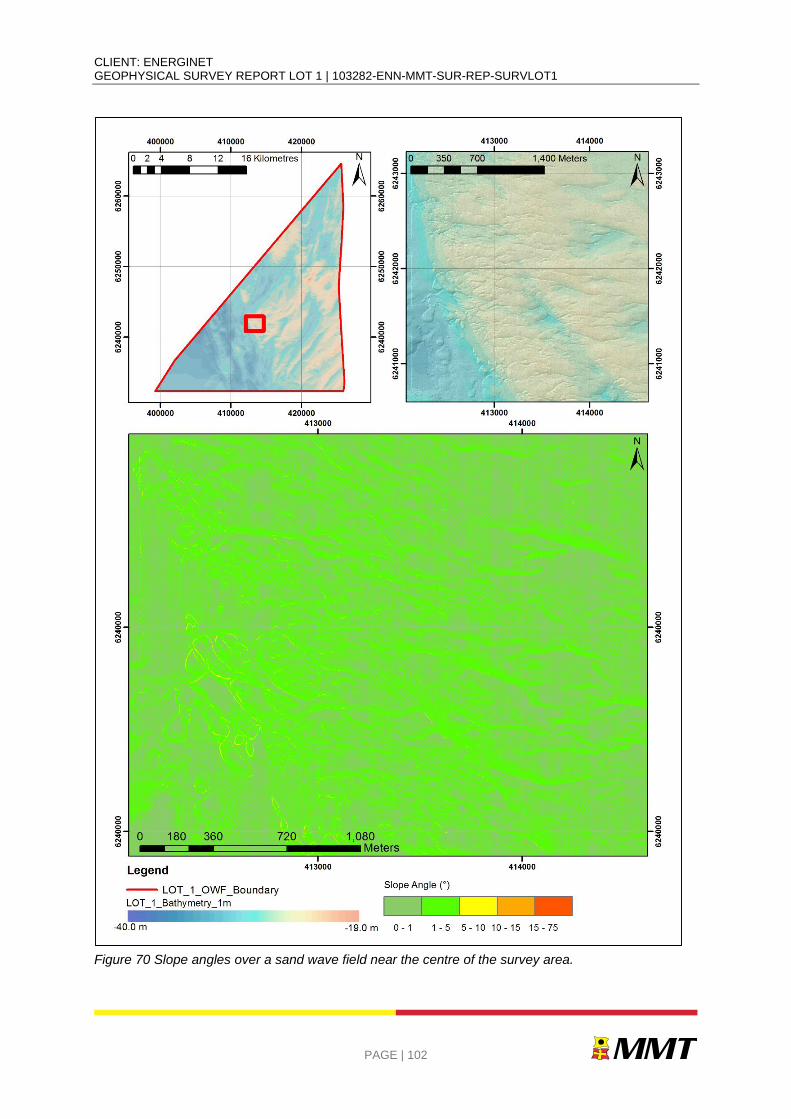
CLIENT: ENERGINET GEOPHYSICAL SURVEY REPORT LOT 1 | 103282-ENN-MMT-SUR-REP-SURVLOT1
PAGE | 102
Figure 70 Slope angles over a sand wave field near the centre of the survey area.
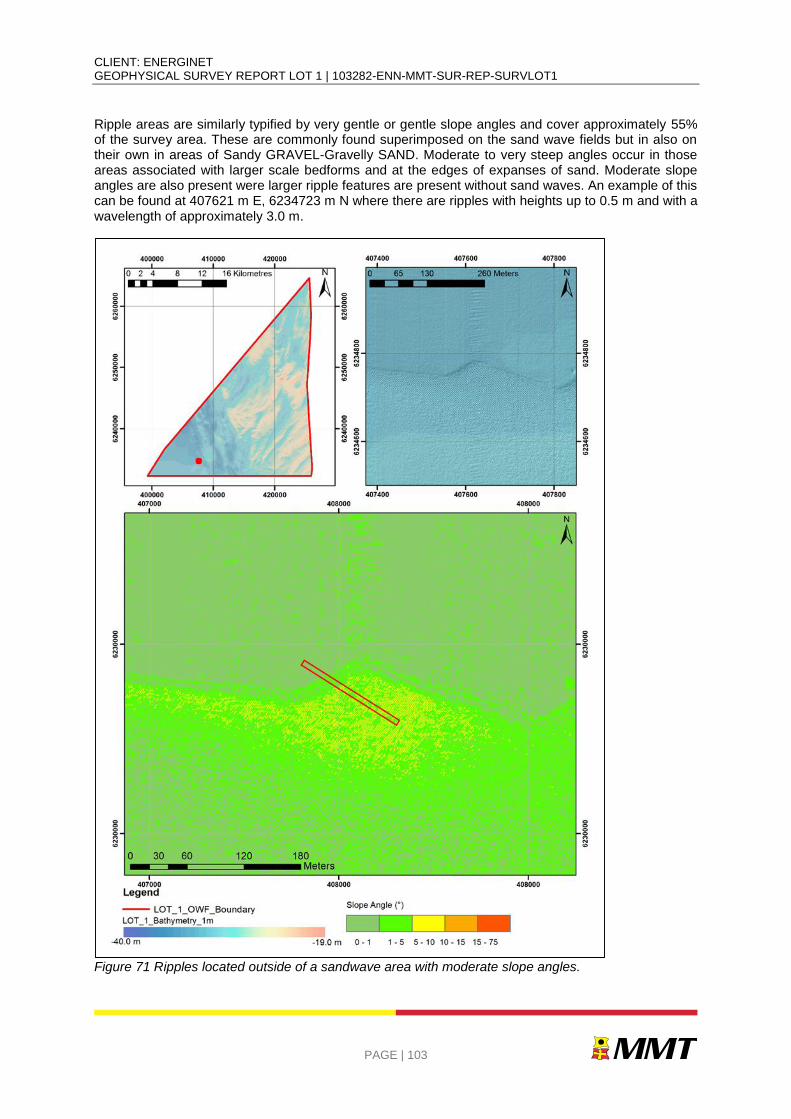
CLIENT: ENERGINET GEOPHYSICAL SURVEY REPORT LOT 1 | 103282-ENN-MMT-SUR-REP-SURVLOT1
PAGE | 103
Ripple areas are similarly typified by very gentle or gentle slope angles and cover approximately 55% of the survey area. These are commonly found superimposed on the sand wave fields but in also on their own in areas of Sandy GRAVEL-Gravelly SAND. Moderate to very steep angles occur in those areas associated with larger scale bedforms and at the edges of expanses of sand. Moderate slope angles are also present were larger ripple features are present without sand waves. An example of this can be found at 407621 m E, 6234723 m N where there are ripples with heights up to 0.5 m and with a wavelength of approximately 3.0 m.
Figure 71 Ripples located outside of a sandwave area with moderate slope angles.
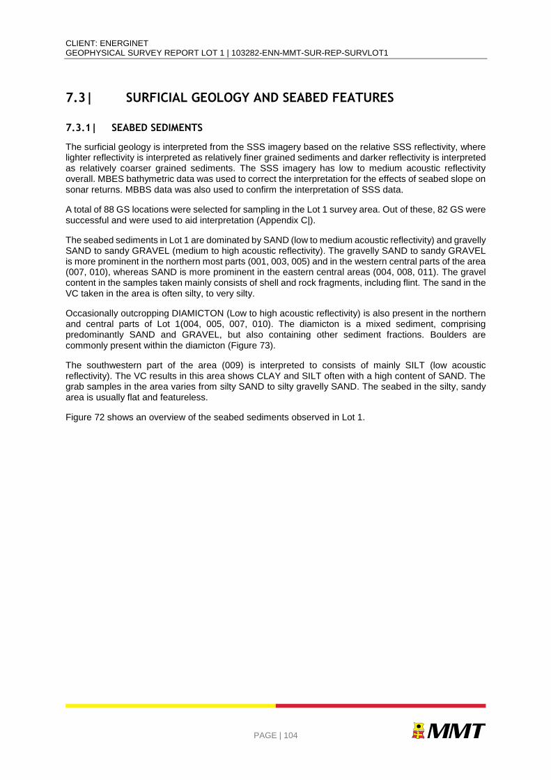
CLIENT: ENERGINET GEOPHYSICAL SURVEY REPORT LOT 1 | 103282-ENN-MMT-SUR-REP-SURVLOT1
PAGE | 104
7.3| SURFICIAL GEOLOGY AND SEABED FEATURES
7.3.1| SEABED SEDIMENTS
The surficial geology is interpreted from the SSS imagery based on the relative SSS reflectivity, where lighter reflectivity is interpreted as relatively finer grained sediments and darker reflectivity is interpreted as relatively coarser grained sediments. The SSS imagery has low to medium acoustic reflectivity overall. MBES bathymetric data was used to correct the interpretation for the effects of seabed slope on sonar returns. MBBS data was also used to confirm the interpretation of SSS data.
A total of 88 GS locations were selected for sampling in the Lot 1 survey area. Out of these, 82 GS were successful and were used to aid interpretation (Appendix C|).
The seabed sediments in Lot 1 are dominated by SAND (low to medium acoustic reflectivity) and gravelly SAND to sandy GRAVEL (medium to high acoustic reflectivity). The gravelly SAND to sandy GRAVEL is more prominent in the northern most parts (001, 003, 005) and in the western central parts of the area (007, 010), whereas SAND is more prominent in the eastern central areas (004, 008, 011). The gravel content in the samples taken mainly consists of shell and rock fragments, including flint. The sand in the VC taken in the area is often silty, to very silty.
Occasionally outcropping DIAMICTON (Low to high acoustic reflectivity) is also present in the northern and central parts of Lot 1(004, 005, 007, 010). The diamicton is a mixed sediment, comprising predominantly SAND and GRAVEL, but also containing other sediment fractions. Boulders are commonly present within the diamicton (Figure 73).
The southwestern part of the area (009) is interpreted to consists of mainly SILT (low acoustic reflectivity). The VC results in this area shows CLAY and SILT often with a high content of SAND. The grab samples in the area varies from silty SAND to silty gravelly SAND. The seabed in the silty, sandy area is usually flat and featureless.
Figure 72 shows an overview of the seabed sediments observed in Lot 1.
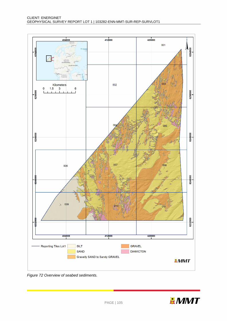
CLIENT: ENERGINET GEOPHYSICAL SURVEY REPORT LOT 1 | 103282-ENN-MMT-SUR-REP-SURVLOT1
PAGE | 105
Figure 72 Overview of seabed sediments.
CLIENT: ENERGINET GEOPHYSICAL SURVEY REPORT LOT 1 | 103282-ENN-MMT-SUR-REP-SURVLOT1
PAGE | 106
Figure 73 SSS example of DIAMICTON (low to high acoustic return).
7.3.2| MOBILE SEDIMENTS
Sand waves and other indications of mobile sediments, such as megaripples and ripples are present in the major parts of the Lot 1 area. The central and northern parts are covered with large areas of sand waves with wave lengths of 100 to 200 m in a south west orientation. Occasional ripples are seen in the troughs between sand waves where gravelly SAND to sandy GRAVEL is present. Occasionally, the ripples are also seen on the sand wave crests. Megaripples are only present in small areas in the central parts of Lot 1 (004, 007, 010). Only the south-westernmost part of the area (009) is featureless with no indications of mobile sediments (Figure 74).
The ripples commonly have a north east / south west direction. (Figure 75, Figure 77). The ripples typically exhibit wave lengths of less than 2 m and are approximately 0.1 to 0.2 m in height and appear in elongated bands in a north – south direction, one noticeable area of ripples can be seen in the south west of Lot 1.
The general direction of transport is from north to south.
CLIENT: ENERGINET GEOPHYSICAL SURVEY REPORT LOT 1 | 103282-ENN-MMT-SUR-REP-SURVLOT1
PAGE | 107
Figure 74 Distribution of sand wave, megaripples and ripples in Lot 1
CLIENT: ENERGINET GEOPHYSICAL SURVEY REPORT LOT 1 | 103282-ENN-MMT-SUR-REP-SURVLOT1
PAGE | 108
Figure 75 76 SSS example of featureless SAND (low acoustic return) and gravelly SAND to sandy GRAVEL with ripples (high acoustic return).
Figure 77 MBES DTM image of SAND and gravelly SAND to sandy GRAVEL with ripples. NaviModel depth convention is positive down, vertical exaggeration of profile is x10. Red box in inset map highlights figure location.
CLIENT: ENERGINET GEOPHYSICAL SURVEY REPORT LOT 1 | 103282-ENN-MMT-SUR-REP-SURVLOT1
PAGE | 109
Associated with mobile sediments are the mass transport deposits occurring mainly in the northern and central parts of the Lot 1 area (003, 004, 005, 007, 010) (Figure 78). These deposits are seen as disturbed sediments often associated with distinct steps in the seabed. They are believed to be caused by slumping of the seabed with succeeding movement of the collapsed sediments, giving varying directions of transport in different locations. The steps caused by the slumping is often associated with high slope values.
Figure 78 Distribution of areas of mass transport deposits in Lot 1.
CLIENT: ENERGINET GEOPHYSICAL SURVEY REPORT LOT 1 | 103282-ENN-MMT-SUR-REP-SURVLOT1
PAGE | 110
7.3.3| AREAS OF DEPRESSIONS
In the eastern and central parts of the survey area, areas of depressions are common (Figure 79, Figure 80) These features are visible as numerous depressions scattered across the seabed and are interpreted to be either caused by changes in seabed current regime or by shallow biogenic gas. Gas charged sediments are seen in the 2D UHRS data, correlating relatively well with these areas indicating a possible gas induced origin (Figure 79). However, these features are also commonly associated with mobile sediments (Figure 80), and at some locations the features are elongated and begins to look like ripples (Figure 81). The origin of the features is therefore uncertain at this point.
Figure 79 Distribution of areas of depressions in relation to sub-surface gas in Lot 1.
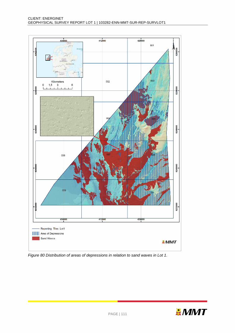
CLIENT: ENERGINET GEOPHYSICAL SURVEY REPORT LOT 1 | 103282-ENN-MMT-SUR-REP-SURVLOT1
PAGE | 111
Figure 80 Distribution of areas of depressions in relation to sand waves in Lot 1.
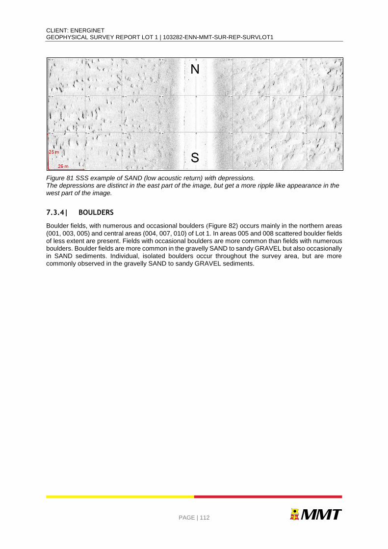
CLIENT: ENERGINET GEOPHYSICAL SURVEY REPORT LOT 1 | 103282-ENN-MMT-SUR-REP-SURVLOT1
PAGE | 112
Figure 81 SSS example of SAND (low acoustic return) with depressions. The depressions are distinct in the east part of the image, but get a more ripple like appearance in the west part of the image.
7.3.4| BOULDERS
Boulder fields, with numerous and occasional boulders (Figure 82) occurs mainly in the northern areas
(001, 003, 005) and central areas (004, 007, 010) of Lot 1. In areas 005 and 008 scattered boulder fields of less extent are present. Fields with occasional boulders are more common than fields with numerous boulders. Boulder fields are more common in the gravelly SAND to sandy GRAVEL but also occasionally in SAND sediments. Individual, isolated boulders occur throughout the survey area, but are more commonly observed in the gravelly SAND to sandy GRAVEL sediments.
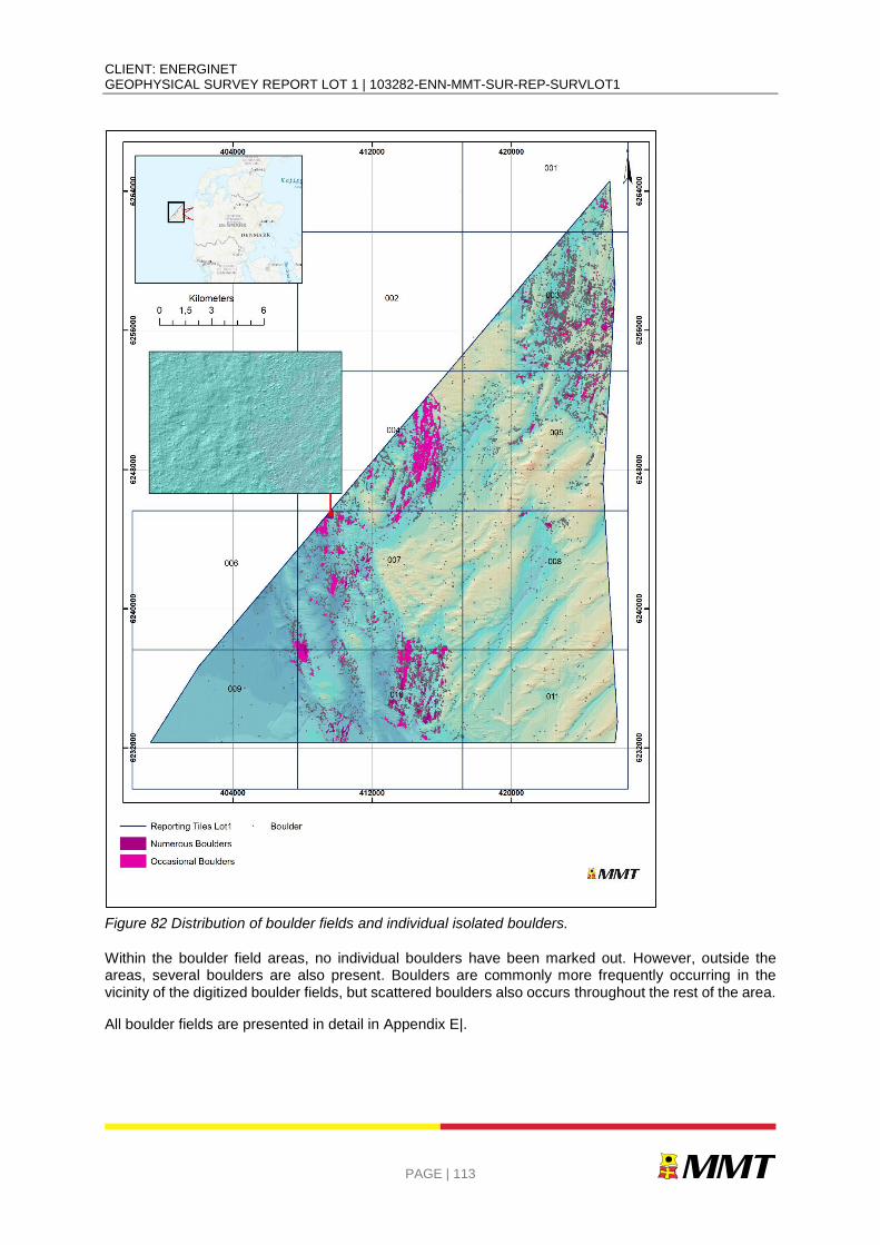
CLIENT: ENERGINET GEOPHYSICAL SURVEY REPORT LOT 1 | 103282-ENN-MMT-SUR-REP-SURVLOT1
PAGE | 113
Figure 82 Distribution of boulder fields and individual isolated boulders.
Within the boulder field areas, no individual boulders have been marked out. However, outside the areas, several boulders are also present. Boulders are commonly more frequently occurring in the vicinity of the digitized boulder fields, but scattered boulders also occurs throughout the rest of the area.
All boulder fields are presented in detail in Appendix E|.

CLIENT: ENERGINET GEOPHYSICAL SURVEY REPORT LOT 1 | 103282-ENN-MMT-SUR-REP-SURVLOT1
PAGE | 114
7.3.5| TRAWL MARKS
Extensive trawl mark areas are found in the south east part of Lot 1 and occasional trawl marks can be seen north of the trawl mark area and in the south west part of Lot 1, (Figure 83 and Figure 84). The observed trawl scars mostly consist of two parallel scars spaced between 15 m to 25 m apart occasional trawl marks are spaced up to 40 m.
Figure 83 Distribution of trawl marks in Lot 1.
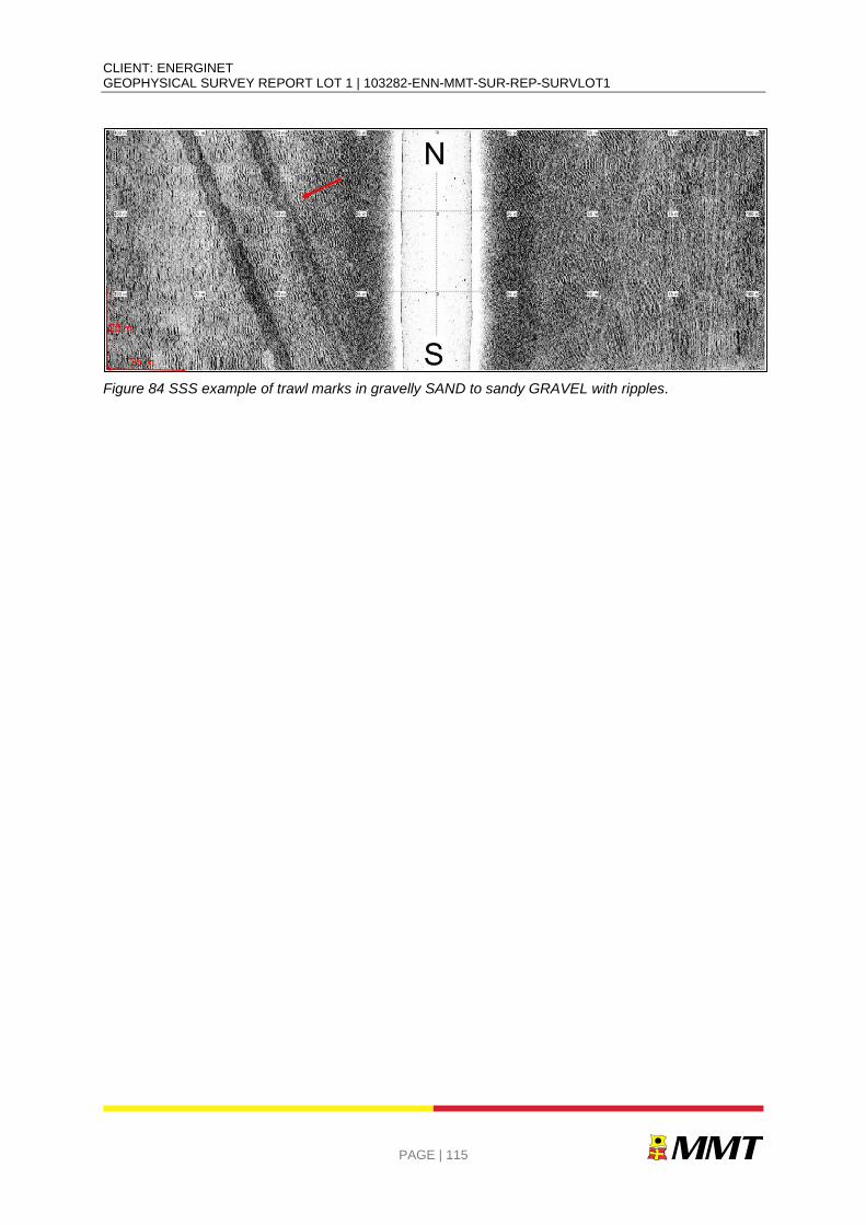
CLIENT: ENERGINET GEOPHYSICAL SURVEY REPORT LOT 1 | 103282-ENN-MMT-SUR-REP-SURVLOT1
PAGE | 115
Figure 84 SSS example of trawl marks in gravelly SAND to sandy GRAVEL with ripples.
CLIENT: ENERGINET GEOPHYSICAL SURVEY REPORT LOT 1 | 103282-ENN-MMT-SUR-REP-SURVLOT1
PAGE | 116
7.4| CONTACTS AND ANOMALIES
In total, 9976 individual seabed contacts and magnetic anomalies were detected in Lot 1. These were detected with SSS, MBES and/or MAG. All seabed objects are detected with either SSS or MBES. All duplicates have been removed. If a SSS or MBES contact were located within 5 m of a MAG anomaly, correlation information was added in the contact listings.
A total of 8096 SSS contacts were detected within Lot 1. They were classified as: wrecks (2), debris (204) and boulders (7890). One of the contacts classified as MMO is considered to be a possible wreck and three classified as MMO are interpreted as wreck debris associated with the wreck due to their close proximity.
The SSS contacts are summarised in Table 22
A total of 1255 MBES contacts were interpreted within Lot 1; MMO (5) and boulders (1250).
MBES contacts are summarised in Table 23
A total of 622 magnetic anomalies were detected in the survey data. No anomalies were associated to known cable and pipeline infrastructure. (see Section 7.5|). The anomalies comprise one wreck and 621 discrete anomalies.
Eight (8) of the discrete anomalies correlates with SSS contacts or MBES contacts. One MAG anomaly (M_103) correlated with a known wreck and also has a correlating SSS contact (S_DH_B03_0559).
Magnetic anomalies are summarised in Table 24.
Full details of all contacts and anomalies are presented in Appendix B|.
Table 22 Summary of SSS contacts.
CLASSIFICATION NUMBER OF CONTACTS
Boulder 7890
MMO 204
Wreck 2
Total 8096
Table 23 Summary of MBES contacts
CLASSIFICATION NUMBER OF CONTACTS
Boulder 1250
MMO 5
Total 1255
Table 24 Summary of magnetic anomalies.
CLASSIFICATION NUMBER OF ANOMALIES
Wreck 1
Discrete 624
Total 625
CLIENT: ENERGINET GEOPHYSICAL SURVEY REPORT LOT 1 | 103282-ENN-MMT-SUR-REP-SURVLOT1
PAGE | 117
7.4.1| WRECKS
Two wrecks were observed within Lot 1. Both wrecks where present in the background data provided by the client.
Wreck S_DH_B01_0199 (400110c_134) was found at 411116 m E, 6242717 m N (Figure 86). No magnetic anomaly was observed in the vicinity. According to background information the ship sank in 1997. The as found dimensions were 8.9 x 2.4 x 0.9 m. Two items of debris were found in the vicinity of the wreck (S_DH_B01_1452 and S_DH_B01_1452).
The wreck S_DH_B03_0559, M_103 (400110c-132) observed within Lot 1 was found at 421836 m E, 6242042 m N (Figure 87) According to background information the ship sank in 1994. The as-found dimensions were 16.2 x 4.7 x 0.7 m.
Table 25 Summary of wrecks (in vicinity of and inside Lot 1), database information.
ID EASTING (m) NORTHING (m) TYPE IN SURVEY
AREA/OBSERVED ON DATA
COMMENT
400110c-10 401830.81 6235889.55 Shipwreck Yes/No Sank in 1979
400110c-55 402822.80 6238717.54 Shipwreck No/No Dated to 1661-2009
400110c-139 403577.81 6235640.56 Shipwreck Yes/No Dated to 1661-2009
400110c-57 406451.79 6234266.58 Shipwreck Yes/No Dated to 1661-2009
400110c-2, 400110c-7; 400110c-1, 400110c-5,
400110c-65, 400110c-4,
400110c-64, 400110c-61, 400110c-60, 400110c-59, 400110c-50, 400110c-49, 400110c-48, 400110c-43, 400110c-36, 400110c-35, 400110c-3
408827.75 6240009.55 Shipwreck Yes/No
Several wrecks at same position in background information. Also parts of wreck and debris associated with wreck..
400110c-11 413262.73 6239353.57 Shipwreck Yes/No Sank in 1979
400110c-134 411113.73 6242719.54 Shipwreck Yes/Yes Sank in 1997. Seen in both MBES and SSS.
400110c-12 411295.73 6244033.54 Shipwreck Yes/No Sank in 1956
400110c-42 418294.69 6241286.57 Shipwreck Yes/No Dated to 1661-2009
400110c-132 421825.67 6242045.58 Shipwreck Yes/Yes Sank in 1994. Seen in SSS, MBES and MAG.
400110c-131 423020.61 6259577.48 Shipwreck Yes/No Sank in 1989
CLIENT: ENERGINET GEOPHYSICAL SURVEY REPORT LOT 1 | 103282-ENN-MMT-SUR-REP-SURVLOT1
PAGE | 118
Figure 85 Overview of wreck locations within and in close vicinity of Lot 1.
CLIENT: ENERGINET GEOPHYSICAL SURVEY REPORT LOT 1 | 103282-ENN-MMT-SUR-REP-SURVLOT1
PAGE | 119
Figure 86 MBES image of wreck S_DH_B01_0199. NaviModel depth convention is positive down, vertical exaggeration of profile is x10. Red box in inset map highlights figure location.
CLIENT: ENERGINET GEOPHYSICAL SURVEY REPORT LOT 1 | 103282-ENN-MMT-SUR-REP-SURVLOT1
PAGE | 120
Figure 87 MBES image of wreck S_DH_B03_0559. NaviModel depth convention is positive down, vertical exaggeration of profile is x10. . Red box in inset map highlights figure location.
7.5| EXISTING INFRASTRUCTURE (CABLES AND PIPELINES)
According to available background data, there are no known cables or pipelines in the area. No cables or pipelines were observed in the survey area.
7.6| SEISMOSTRATIGRAPIC INTERPRETATION
7.6.1| GEOLOGICAL FRAMEWORK
The Danish sector of the North Sea basin is connected to the east sector by the Scandinavian Shield and by the WNW-ESE striking Sorgenfrei-Tornquist fault zone, Figure 88. The Ringkøbing-Fyn High, located further south, emerged during the Late Permian (Pre-Zechstein) as a result of tectonic subsidence (Vejbæk, 1997; Vejbæk et al., 2007). This structural feature divides the Danish sector of the North Sea basin into the North German Basin, located south of the Ringkøbing-Fyn High, and the Danish-Norwegian Basin, north of Ringkøbing-Fyn High. During the Zechstein (Late Permian) four to five cycles of evaporites were deposited, infilling the structural lows (Sorgenfrei and Buch, 1964; Vejbæk et al., 2007). Further deepening of the North Sea basin resulted in thousands of metres of Mesozoic sediment deposition over the evaporites. The thick Mesozoic deposits activated diapirism of the underlying evaporites. Subsequently, several cycles of glaciations resulted in further loading inducing

CLIENT: ENERGINET GEOPHYSICAL SURVEY REPORT LOT 1 | 103282-ENN-MMT-SUR-REP-SURVLOT1
PAGE | 121
reactivation and upward migration of the salt diapirs (Nielsen et al., 2008). This halokinesis is likely to be ongoing in modern times.
Figure 88 Major Danish structural elements (After Stemmerik et al., 2000); site location in red.
During the Late Cretaceous a major tectonic inversion episode, associated with initiation of the Alpine Orogeny, affected the North Sea region (Clausen and Huuse, 1999; Japsen, 2000). Cretaceous tectonism was followed by sequential episodes of uplift and major sea level fluctuations from the Paleogene to Neogene. These events resulted in variable rates and types of sediment deposition. The top of the Paleogene-Neogene succession is represented as an important unconformity in Denmark. The same unconformity corresponds to the base of the Quaternary as defined in Rasmussen et al. (2010). The Pre-Quaternary deposits are successively younger moving from the rim of the basin at the Sorgenfrei-Tornquist Zone towards the central North Sea Basin. The depositional systems (mostly deltaic) show a general shift moving from east to west. The Miocene succession is hundreds of metres thick in the Danish sector of the North Sea. A major regional unconformity occurs between the Upper Eocene and lower Upper Oligocene, Brejning Fm. (Mica Clay) (Rasmussen et al., 2010).
A large-scale glaciotectonic thrust complex has been identified in the Danish sector of the North Sea and it is bounded at is base by a weak décollement surface (Larsen and Andersen, 2005). The décollement surface is located in the early Miocene Arnum Formation (Andersen, 2004). It is interpreted
CLIENT: ENERGINET GEOPHYSICAL SURVEY REPORT LOT 1 | 103282-ENN-MMT-SUR-REP-SURVLOT1
PAGE | 122
as being of glaciotectonic origin (Huuse and Lykke-Andersen, 2000b; Andersen, 2004). The deformed sequence located above this structure comprises sediments from the Miocene to the Quaternary. Correlation with onshore areas suggest that the deformation took place during a westward advance stage of the Late Saalian (Warthe) ice sheet (Andersen, 2004). Based on the glacial stratigraphy outside the deformed areas (away from the deformation front), it is suggested that the same ice sheet advance that caused the glaciotectonic deformation eroded the top of the thrust sheets (Larsen and Andersen, 2005).
Nielsen et al. (2008) states that Quaternary sequences rest conformably on Pliocene deltaic sediments west of a transitional zone in the North Sea (Figure 89). East of the transition zone, the base of the Quaternary rises, becoming an unconformity along the coast from north of Thyborøn to south of the Danish-German border (e.g. Japsen, 2000; Nielsen et al., 2008). Generally, this unconformity (base of Quaternary) occurs at depths of a few hundred metres within valley structures to just below the seabed along the Danish west coast (Andersen, 2004; Huuse and Lykke-Andersen, 2000b; Leth et al., 2004, Novak et al., 2015). Across the wider region this surface is characterized by strong undulation controlled by variable-scale structures in the pre-Quaternary basement.
Figure 89 Regional geological map (After Nielsen et al., 2008); site location in red.
Only a few studies have been performed on the Quaternary deposits in the Danish North Sea. However, onshore studies provide a decent foundation for outlining the regional geology in the eastern North Sea

CLIENT: ENERGINET GEOPHYSICAL SURVEY REPORT LOT 1 | 103282-ENN-MMT-SUR-REP-SURVLOT1
PAGE | 123
(Sjørring and Frederiksen, 1980; Sandersen and Jørgensen, 2003; Pedersen, 2005; Jørgensen and Sandersen, 2006; Jacobsen, 2003; Høyer A-S et al., 2013; Houmark-Nielsen, 2007).
The Elster and Saale ice sheets extended across the entire North Sea (Figure 90). Glaciation came from the northwest, northeast and from the Baltic region (Sjørring and Frederiksen, 1980; Ehlers, 1990). The Weichselian ice sheet extended north and east of the main stationary line which was located from inland Jutland towards the northwest into the North Sea. Morphological elements such as moraine ridges and elongated boulder reefs, occurring perpendicular to the main stationary line, indicate the location of the ice boundary on the seabed (Nicolaisen, 2010). The maximum extent of the ice extended further than the site during the Elsterian and Saalian glacial periods, being the site in a sub glacial setting for those periods. For the Weichselian glacial period, the maximum extent of the ice sheet was close to the site, however the available references do not have it extending over the site. Therefore, it was presumably in a proglacial environment for the Last Glacial Maximum (LGM).
CLIENT: ENERGINET GEOPHYSICAL SURVEY REPORT LOT 1 | 103282-ENN-MMT-SUR-REP-SURVLOT1
PAGE | 124
Figure 90 The quaternary glaciations and an overview of Quaternary valleys in northwest Europe. (Huuse, M., and Lykke-Andersen, H. 2000); site location in red.
In general, the Quaternary sequence thins from the central North Sea towards the Danish mainland (from thousands to tens of metres thick). A system of buried shelf valleys, 100-300m deep and several

CLIENT: ENERGINET GEOPHYSICAL SURVEY REPORT LOT 1 | 103282-ENN-MMT-SUR-REP-SURVLOT1
PAGE | 125
tens of kilometres long, are present in this area (Andersen, 2004; Huuse and Lykke-Andersen, 2000b; Novak et al., 2015). The submarine valleys are correlatable to onshore valleys and are considered to be of the Elster and Saale ages. Younger, reactivated Saale valleys have been found north and east of the Weichselian main stationary line (Smed 1979, 1981a; Jørgensen et al., 2005). Repeated episodes of glacial advance and catastrophic outbursts of melt water are believed to be the processes that generated these valleys.
Pre-Weichselian glaciations are not well documented offshore along the Danish west coast. However, it is known that the Elster and Saale ice sheets covered the Danish North Sea and extended further to the south (Ehlers, 1990). The formation of glacial tectonic complexes found to the west and south of the Weichselian ice sheet at the LGM boundary are believed to be attributable to the Saalian ice cover (Andersen, 2004; Huuse and Lykke-Andersen, 2000b; Novak et al., 2015; Vaughan-Hirsch and Phillips, 2017). In the Holmsland Thrust Complex (Novak et al., 2015) Saale till was found in a borehole at approximately 60 metres below sea level (Fugro 2014).
Onshore, the so called "hill islands" (Dalgas, 1867), which outline the Saalian landscape, are found to extend into the North Sea (Larsen, 2003; Larsen & Andersen, 2006, Leth et al., 2001; Anthony, 2001; Leth, 2003). Morphological remnants are absent on the seabed due to marine erosion. However, seismic profiles reveal horizons that have been interpreted to represent this same landscape.
During the Eemian period the Paleo-North Sea extended across the region. Related sediment deposits occur both on and offshore in the southwest (Konradi et al., 2005). Eem deposits representing valley infill were found in a borehole in the Vesterhav South survey area (Fugro 2014).
During the Weichselian glaciations, Figure 91, tills alternate with mixed sediment units comprised of glaciofluvial gravel, glaciolacustrine clay, silt and sand that were deposited to the north and east of the main stationary line. Towards the west and south of the main stationary line, glaciofluvial sand and gravel were deposited in morphological lows within the older Saale landscape (Houmark-Nielsen, 2007). The glaciation maximum occurred in the region around 22ka BP. The glaciers´ subsequent retreat generated accommodation space close to the ice front where deposition of the glaciolacustrine Yoldia Clay occurred around 16-15ka BP. Also, as Weichselian ice melted, the deep-valleys were filled with laminated clay, silt and fine sand deposits, Figure 91.
CLIENT: ENERGINET GEOPHYSICAL SURVEY REPORT LOT 1 | 103282-ENN-MMT-SUR-REP-SURVLOT1
PAGE | 126
Figure 91 General stratigraphy model of the geology in the eastern Danish North Sea. A composite profile from NW towards SE representing approximately 50 km from Jyske Rev and towards the shore. Below: Stratigraphic unit names and their relative age. Same colour code used above and below. (After Nicolaisen, 2010).
CLIENT: ENERGINET GEOPHYSICAL SURVEY REPORT LOT 1 | 103282-ENN-MMT-SUR-REP-SURVLOT1
PAGE | 127
The removal of the glacial load triggered isostatic rebound which drove a regression that took place until 11ka BP. During this timeframe, relative sea level was, at a minimum, 50 to 45 metres lower than present thus maintaining the eastern Danish shelf above sea level. Terrestrial conditions and rising temperatures increased organic material production resulting in peat accumulations. This marker horizon has been found in many survey areas across Danish waters (Leth, 1996; Bennike et al., 1998, 2000; Novak and Björck, 2002; Novak and Pedersen, 2000). In the eastern Danish North Sea fine-grained material was deposited in sheltered areas between till "islands", e.g, the Agger Clay unit (Leth, 1996). During the Holocene transgression, from 11ka BP to 6 ka BP, the Agger Clay depocenter shifted coastward and offshore low-lying islands were submerged. At the same time, coastal processes overtook the glaciogenic landscape where it was exposed to waves and currents. The result was the formation of spit/platform/lagoon deposits throughout the region (Nielsen and Johannesen, 2004; Johannesen et al., 2008; Novak and Pedersen, 2000).
In the eastern North Sea, metre-thick fossil sand waves were present at Jyske Rev. These current- and wave-generated structures have often been formed around sandy-gravelly fossil beach ridges. Seismic data depict multiple generations of these events. After 6 ka BP sea level was at its highest and the North Sea tidal system and coast parallel Jylland current developed.
A recent mobile sediment unit is the latest deposit and is found to cover major areas of the eastern North
Sea seabed. Coast-parallel strong currents and waves generate the active bedforms, i.e., mobile sand
waves and dunes. The Danish Coast Agency has documented bedform migrations of up to 20-50m per
year; the dunes and waves are organized in kilometre-wide areas migrating across an apron of relict
gravelly sand (Anthony and Møller, 2003; Anthony and Leth, 2001; Leth et al., 2004).
7.6.2| SUB-SEABED GEOLOGY – GEOMODEL
The seismostratigraphic interpretation carried out for this project is based on eight mapped horizons.
Units are described herein according to their base geometries, seismic facies and internal reflections, emphasizing that seismostratigraphic boundaries have a chronostratigraphic meaning and should not be interpreted in lithostratigraphic terms. An exception is T99, mapped as top, and therefore has no chronostratigraphic meaning.
All figures and seismic interpretation work that are included in this report are part of the Kingdom Suite project that was sent at the time of the FULL TRACK delivery. All seismic profiles are FULL-processed, migrated and in depth (metres). Numbers on the horizontal axis refer to distance in metres, numbers on the vertical axis correspond to metres. The colorbar for the seismic display is identical for all profiles (‘Black to White 200’ in Kingdom Suite). The colorbar used to show the lateral extension for each basemap is the 3D Effects: warm colours (red) indicate shallower depths, and cool colours (blue) indicate greater depths.
For every unit, three basemaps are presented: (1) spatial extent of the mapped horizon, (2) grid of the depth below seabed of the base of the unit, (3) grid of the thickness of the unit. Included in the Kingdom Suite project are all horizons and grids for all horizons, and horizons of shallow gas and hazards mapped within the site. For the final delivery all seismic sections, basemaps and thickness will be available in depth-domain (metres).
Vibrocore data was used for interpretation purposes as it ties seismostratigraphic units with lithostratigraphic information. Vibrocores data was integration in Kingdom Suite as “Formations Tops”. Some adjustments were done to tie with the water depth and the MBES data.
UHRS profiles presented in Figure 92, are examples of the seismostratigraphic interpretation and the proposed mapped horizons, as well as their respective colours. Figure 92 below summarises the seismic units, their boundaries, the nature of the base, seismic facies and geological significance.
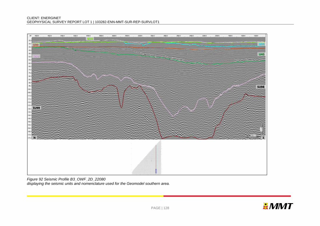
CLIENT: ENERGINET GEOPHYSICAL SURVEY REPORT LOT 1 | 103282-ENN-MMT-SUR-REP-SURVLOT1
PAGE | 128
Figure 92 Seismic Profile B3_OWF_2D_22080 displaying the seismic units and nomenclature used for the Geomodel southern area.
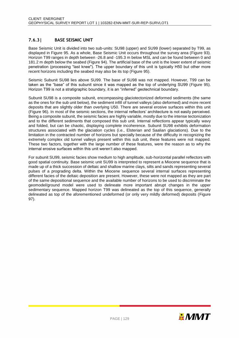
CLIENT: ENERGINET GEOPHYSICAL SURVEY REPORT LOT 1 | 103282-ENN-MMT-SUR-REP-SURVLOT1
PAGE | 129
7.6.3| BASE SEISMIC UNIT
Base Seismic Unit is divided into two sub-units: SU98 (upper) and SU99 (lower) separated by T99, as displayed in Figure 95. As a whole, Base Seismic Unit occurs throughout the survey area (Figure 93). Horizon T99 ranges in depth between -26.8 and -195.3 m below MSL and can be found between 0 and 181.2 m depth below the seabed (Figure 94). The artificial base of the unit is the lower extent of seismic penetration (processing “last knee"). The upper boundary of this unit is typically H50 but other more recent horizons including the seabed may also be its top (Figure 95).
Seismic Subunit SU98 lies above SU99. The base of SU98 was not mapped. However, T99 can be taken as the “base” of this subunit since it was mapped as the top of underlying SU99 (Figure 95). Horizon T99 is not a stratigraphic boundary, it is an “inferred” geotechnical boundary.
Subunit SU98 is a composite subunit, encompassing glaciotectonized deformed sediments (the same as the ones for the sub unit below), the sediment infill of tunnel valleys (also deformed) and more recent deposits that are slightly older than overlying U50. There are several erosive surfaces within this unit (Figure 96). In most of the seismic sections, the internal reflectors’ architecture is not easily perceived. Being a composite subunit, the seismic facies are highly variable, mostly due to the intense tectonization and to the different sediments that composed this sub unit. Internal reflections appear typically wavy and folded, but can be chaotic, displaying complete incoherence. Subunit SU98 exhibits deformation structures associated with the glaciation cycles (i.e., Elsterian and Saalian glaciations). Due to the limitation in the contracted number of horizons but specially because of the difficulty in recognizing the extremely complex old tunnel valleys present within this sub unit, these features were not mapped. These two factors, together with the large number of these features, were the reason as to why the internal erosive surfaces within this unit weren’t also mapped.
For subunit SU99, seismic facies show medium to high amplitude, sub-horizontal parallel reflectors with good spatial continuity. Base seismic unit SU99 is interpreted to represent a Miocene sequence that is made up of a thick succession of deltaic and shallow marine clays, silts and sands representing several pulses of a prograding delta. Within the Miocene sequence several internal surfaces representing different facies of the deltaic deposition are present. However, these were not mapped as they are part of the same depositional sequence and the available number of horizons to be used to discriminate the geomodel/ground model were used to delineate more important abrupt changes in the upper sedimentary sequence. Mapped horizon T99 was delineated as the top of this sequence, generally delineated as top of the aforementioned undeformed (or only very mildly deformed) deposits (Figure 97).
CLIENT: ENERGINET GEOPHYSICAL SURVEY REPORT LOT 1 | 103282-ENN-MMT-SUR-REP-SURVLOT1
PAGE | 130
Figure 93 Map showing the lateral extent of T99 (The horizon that delineates the top of SU99 and separates SU99 and SU98). Units in metres below MSL.
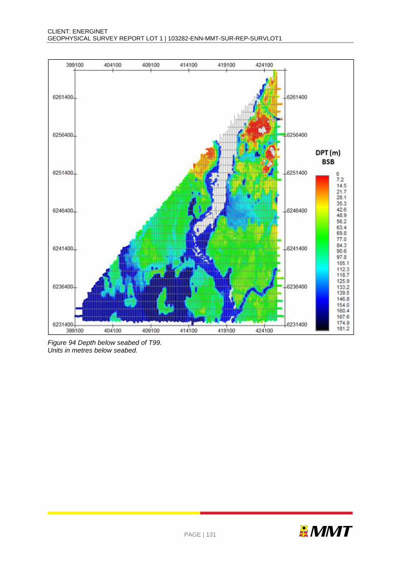
CLIENT: ENERGINET GEOPHYSICAL SURVEY REPORT LOT 1 | 103282-ENN-MMT-SUR-REP-SURVLOT1
PAGE | 131
Figure 94 Depth below seabed of T99. Units in metres below seabed.
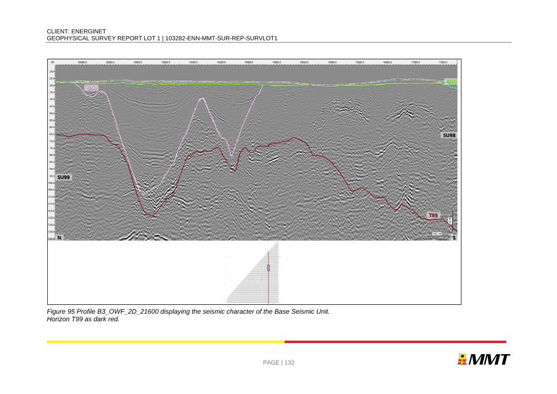
CLIENT: ENERGINET GEOPHYSICAL SURVEY REPORT LOT 1 | 103282-ENN-MMT-SUR-REP-SURVLOT1
PAGE | 132
Figure 95 Profile B3_OWF_2D_21600 displaying the seismic character of the Base Seismic Unit. Horizon T99 as dark red.
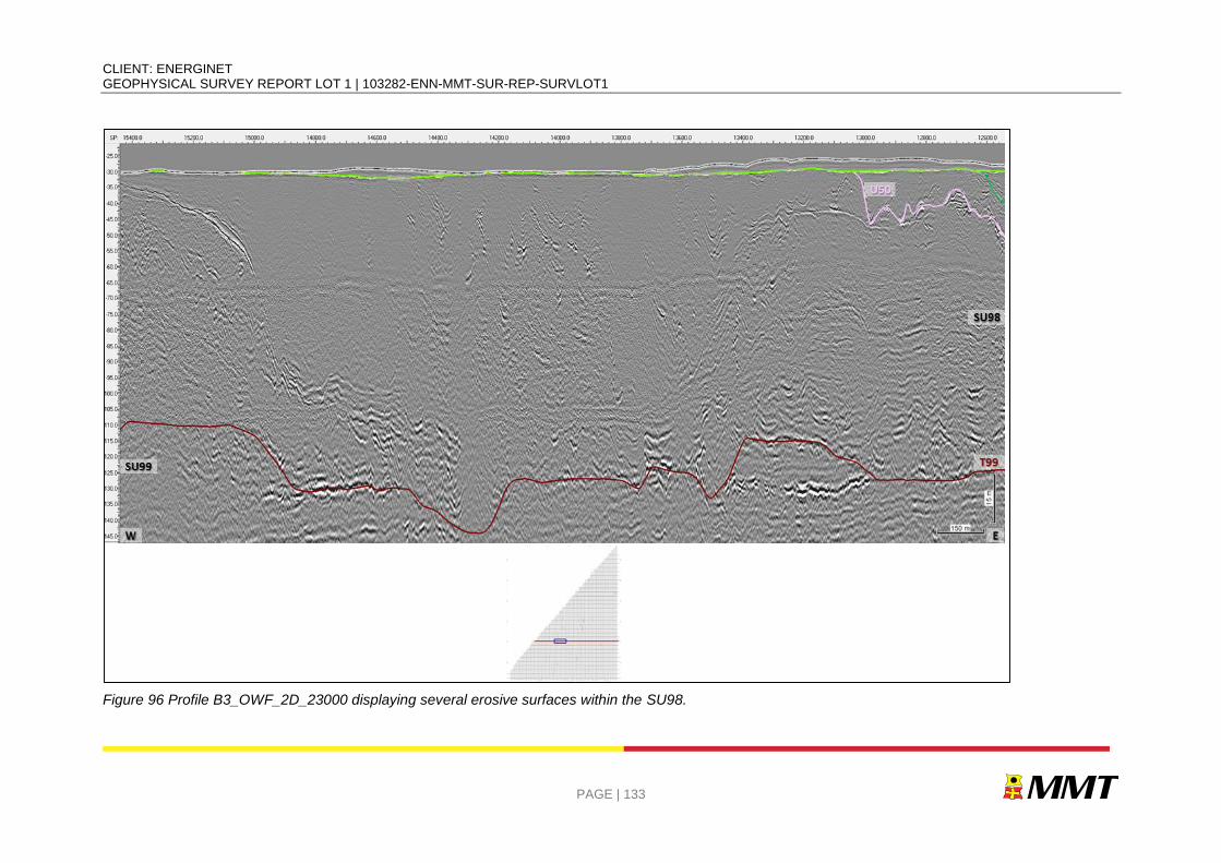
CLIENT: ENERGINET GEOPHYSICAL SURVEY REPORT LOT 1 | 103282-ENN-MMT-SUR-REP-SURVLOT1
PAGE | 133
Figure 96 Profile B3_OWF_2D_23000 displaying several erosive surfaces within the SU98.
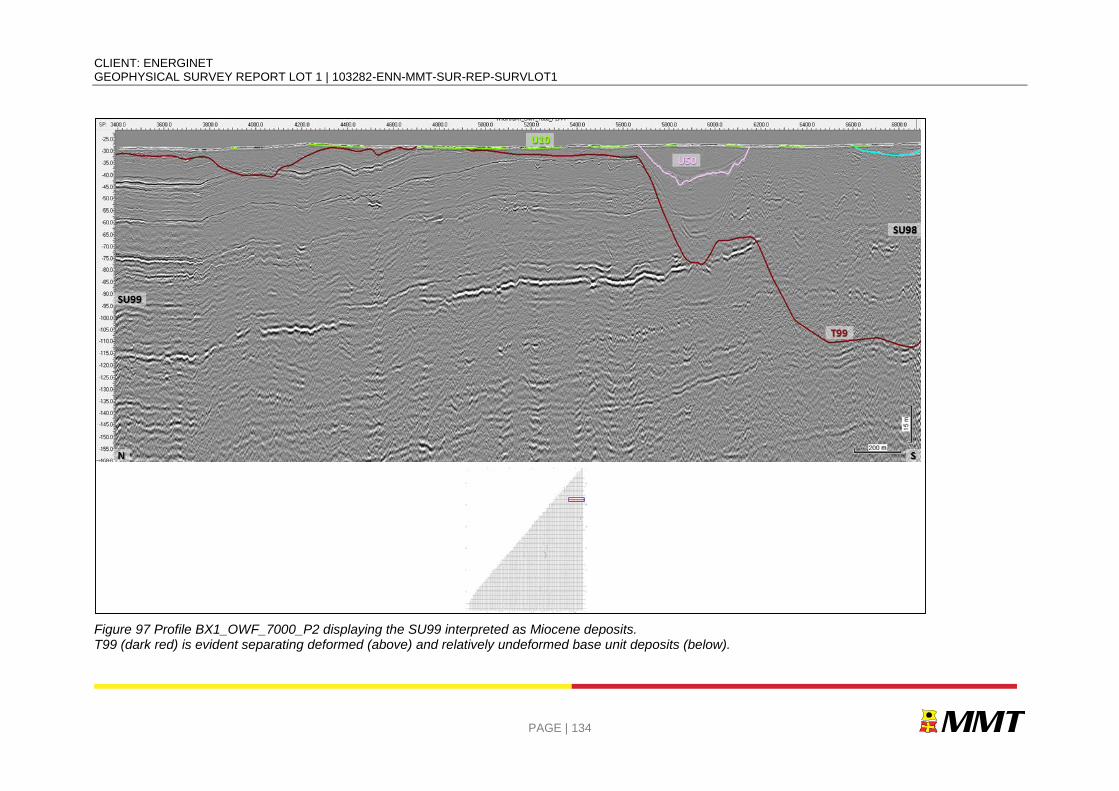
CLIENT: ENERGINET GEOPHYSICAL SURVEY REPORT LOT 1 | 103282-ENN-MMT-SUR-REP-SURVLOT1
PAGE | 134
Figure 97 Profile BX1_OWF_7000_P2 displaying the SU99 interpreted as Miocene deposits. T99 (dark red) is evident separating deformed (above) and relatively undeformed base unit deposits (below).

CLIENT: ENERGINET GEOPHYSICAL SURVEY REPORT LOT 1 | 103282-ENN-MMT-SUR-REP-SURVLOT1
PAGE | 135
7.6.4| SEISMIC UNIT U50 – LIGHT PINK
Seismic unit U50 occurs in the central and eastern part of the survey area (Figure 98). The base H50 has irregular geometry, with pronounced undulations, resembling a network of carved channels several kilometres wide (Figure 101 and Figure 102). In a part of the area (north segment of the major incised valley axis), H50 becomes the processing last knee. Horizon H50 ranges in depth between -26.7 and -166.8 m below MSL. The base of unit U50 is found between 0 and 156.3 m depth below the seabed (Figure 99). The thickness of U50 ranges from 0 to 153.2 m. U50 is thickest in the deeply incised valley axis. (Figure 100).
The seismic facies of U50 is well-organised, with (sub) parallel reflectors with good spatial continuity and fine layering. The seismic facies and reflector characteristics of U50 suggest a relatively low-energy depositional environment with mud and fine sands infilling tunnel valleys (Figure 101). Figure 102 displays different seismic facies for this unit, that is present in the top package for U50. It displays less organised reflectors, slightly wavier, dipping and with a divergent pattern. The tunnel valleys could be associated with the Elsterian and Saalian glaciations. Presence of shallow gas is observed in this unit (Figure 103).
SU98 is made of a thick package of very fine laminated deposits. This was one of the most important criteria to delineate and map this seismic unit. It is possible that this unit is present in some areas without this typical seismic character (most likely to superimposed deformation). In those instances, the deposits were incorporated as SU98 (Figure 104).
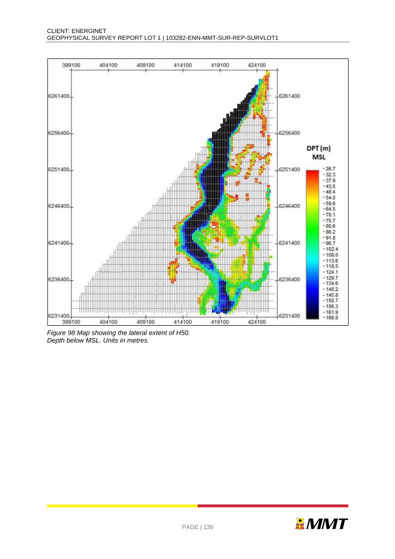
CLIENT: ENERGINET GEOPHYSICAL SURVEY REPORT LOT 1 | 103282-ENN-MMT-SUR-REP-SURVLOT1
PAGE | 136
Figure 98 Map showing the lateral extent of H50. Depth below MSL. Units in metres.
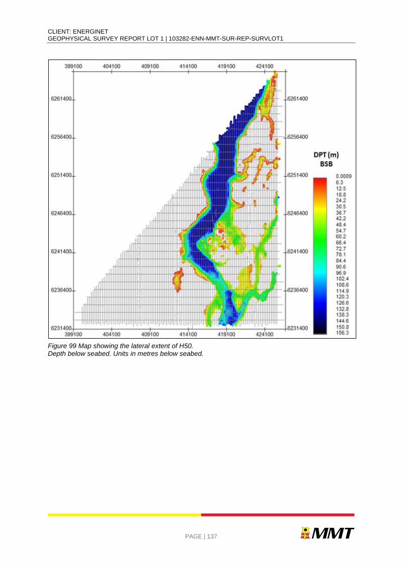
CLIENT: ENERGINET GEOPHYSICAL SURVEY REPORT LOT 1 | 103282-ENN-MMT-SUR-REP-SURVLOT1
PAGE | 137
Figure 99 Map showing the lateral extent of H50. Depth below seabed. Units in metres below seabed.
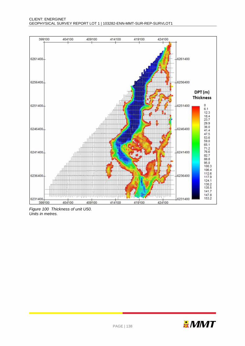
CLIENT: ENERGINET GEOPHYSICAL SURVEY REPORT LOT 1 | 103282-ENN-MMT-SUR-REP-SURVLOT1
PAGE | 138
Figure 100 Thickness of unit U50. Units in metres.

CLIENT: ENERGINET GEOPHYSICAL SURVEY REPORT LOT 1 | 103282-ENN-MMT-SUR-REP-SURVLOT1
PAGE | 139
Figure 101 Profile B2_OWF_2D_17040 Displaying subparallel, slightly divergent well-organized seismic facies for Unit U50, horizon H50 (light pink).
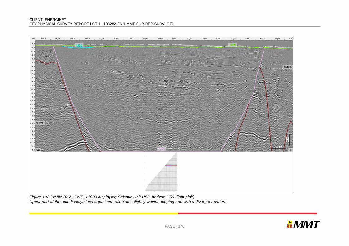
CLIENT: ENERGINET GEOPHYSICAL SURVEY REPORT LOT 1 | 103282-ENN-MMT-SUR-REP-SURVLOT1
PAGE | 140
Figure 102 Profile BX2_OWF_11000 displaying Seismic Unit U50, horizon H50 (light pink). Upper part of the unit displays less organized reflectors, slightly wavier, dipping and with a divergent pattern.
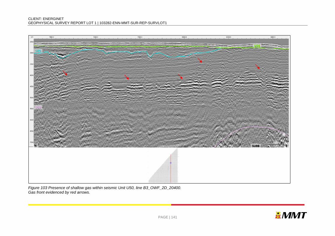
CLIENT: ENERGINET GEOPHYSICAL SURVEY REPORT LOT 1 | 103282-ENN-MMT-SUR-REP-SURVLOT1
PAGE | 141
Figure 103 Presence of shallow gas within seismic Unit U50, line B3_OWF_2D_20400. Gas front evidenced by red arrows.
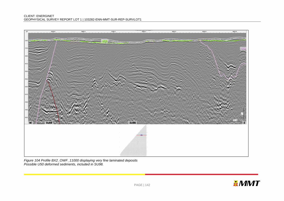
CLIENT: ENERGINET GEOPHYSICAL SURVEY REPORT LOT 1 | 103282-ENN-MMT-SUR-REP-SURVLOT1
PAGE | 142
Figure 104 Profile BX2_OWF_11000 displaying very fine laminated deposits Possible U50 deformed sediments, included in SU98.
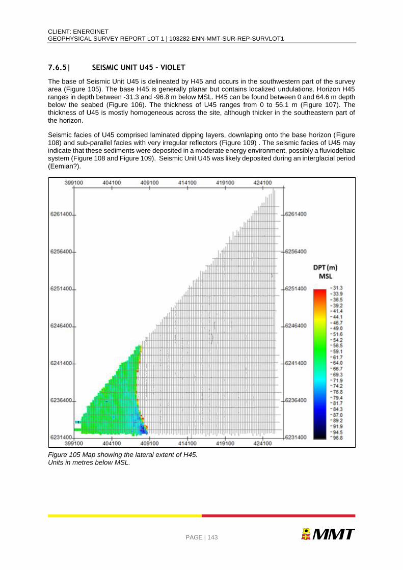
CLIENT: ENERGINET GEOPHYSICAL SURVEY REPORT LOT 1 | 103282-ENN-MMT-SUR-REP-SURVLOT1
PAGE | 143
7.6.5| SEISMIC UNIT U45 – VIOLET
The base of Seismic Unit U45 is delineated by H45 and occurs in the southwestern part of the survey area (Figure 105). The base H45 is generally planar but contains localized undulations. Horizon H45 ranges in depth between -31.3 and -96.8 m below MSL. H45 can be found between 0 and 64.6 m depth below the seabed (Figure 106). The thickness of U45 ranges from 0 to 56.1 m (Figure 107). The thickness of U45 is mostly homogeneous across the site, although thicker in the southeastern part of the horizon.
Seismic facies of U45 comprised laminated dipping layers, downlaping onto the base horizon (Figure 108) and sub-parallel facies with very irregular reflectors (Figure 109) . The seismic facies of U45 may indicate that these sediments were deposited in a moderate energy environment, possibly a fluviodeltaic system (Figure 108 and Figure 109). Seismic Unit U45 was likely deposited during an interglacial period (Eemian?).
Figure 105 Map showing the lateral extent of H45. Units in metres below MSL.
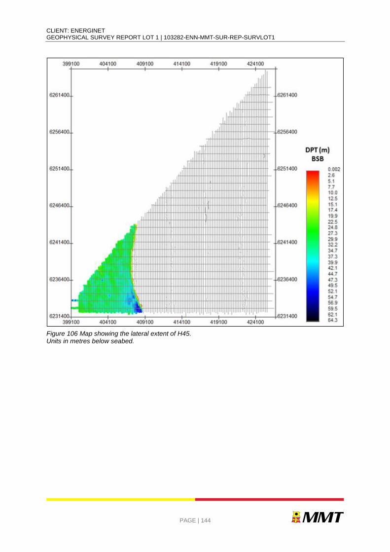
CLIENT: ENERGINET GEOPHYSICAL SURVEY REPORT LOT 1 | 103282-ENN-MMT-SUR-REP-SURVLOT1
PAGE | 144
Figure 106 Map showing the lateral extent of H45. Units in metres below seabed.
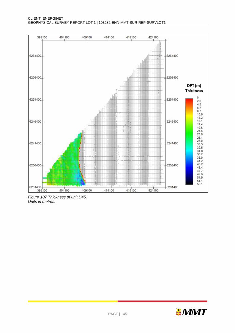
CLIENT: ENERGINET GEOPHYSICAL SURVEY REPORT LOT 1 | 103282-ENN-MMT-SUR-REP-SURVLOT1
PAGE | 145
Figure 107 Thickness of unit U45. Units in metres.
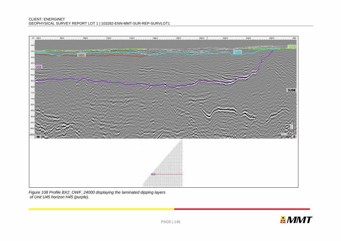
CLIENT: ENERGINET GEOPHYSICAL SURVEY REPORT LOT 1 | 103282-ENN-MMT-SUR-REP-SURVLOT1
PAGE | 146
Figure 108 Profile BX2_OWF_24000 displaying the laminated dipping layers of Unit U45 horizon H45 (purple).
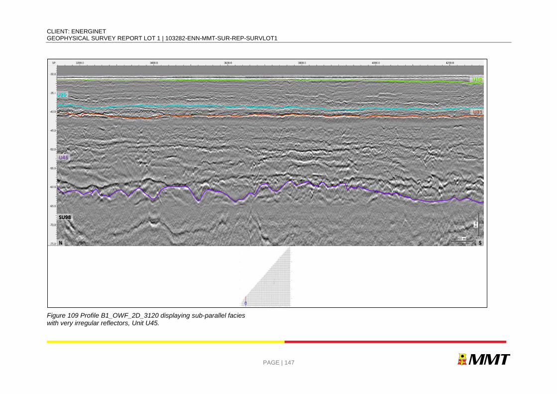
CLIENT: ENERGINET GEOPHYSICAL SURVEY REPORT LOT 1 | 103282-ENN-MMT-SUR-REP-SURVLOT1
PAGE | 147
Figure 109 Profile B1_OWF_2D_3120 displaying sub-parallel facies with very irregular reflectors, Unit U45.

CLIENT: ENERGINET GEOPHYSICAL SURVEY REPORT LOT 1 | 103282-ENN-MMT-SUR-REP-SURVLOT1
PAGE | 148
7.6.6| SEISMIC UNIT U40 – SPRING GREEN
The base of Seismic Unit U40 is delineated by H40 and occurs in the southeastern part of the survey area (Figure 110). H40 traces an irregular and undulated reflector across the area. Horizon H40 ranges in depth between -26.3 and -107.1 m below MSL. H40 can be found between 0 and 80.0 m depth below the seabed (Figure 111). The thickness of U40 ranges from 0 to 58.3 m (Figure 112).
The organisation of acoustic stratigraphy within U40 varies from the bottom to top, displaying a range of seismic facies (Figure 113, Figure 114 and Figure 115). The base of U40 shows transparent and chaotic reflections (Figure 114) and marks the beginning of a different regime of sedimentation, probably with more coarse sediments. Channelization is evident within U40. An internal erosive surface is present, and is recognised by an irregular and very undulated geometry traced by a high amplitude reflector (Figure 113). The irregular and strong reflector can be related with presence of organic material or even charge with gas. The upper part of the unit is likely associated to a relatively moderate energy environment transitioning to a lower energy environment towards the top, possibly glaciolacustrine. The upper part of this unit shows sub-parallel, wavy and continuous reflections with moderate amplitude (Figure 113, Figure 114 and Figure 115).
This unit is likely associated with a glaciolacustrine or a similar relatively low-energy environment.
Seismic Unit U40 could have been deposited during a glacial period (Weichselian?).
Shallow gas is present within this unit (Figure 116).
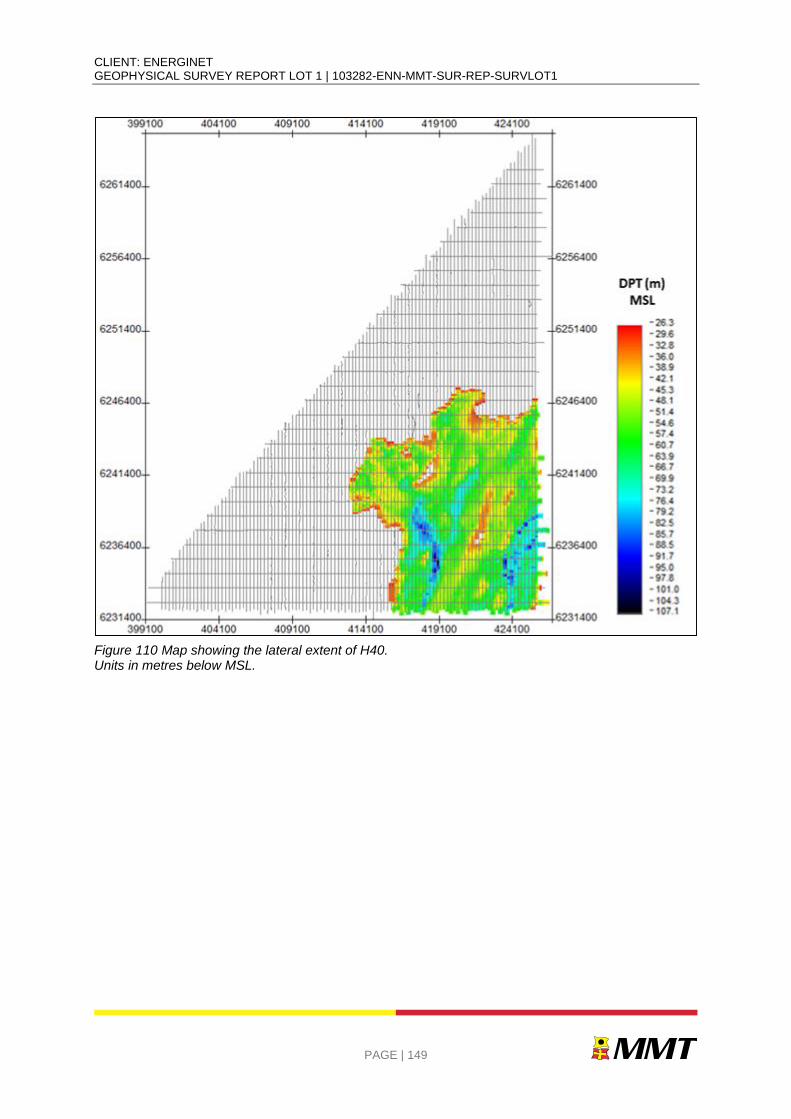
CLIENT: ENERGINET GEOPHYSICAL SURVEY REPORT LOT 1 | 103282-ENN-MMT-SUR-REP-SURVLOT1
PAGE | 149
Figure 110 Map showing the lateral extent of H40. Units in metres below MSL.
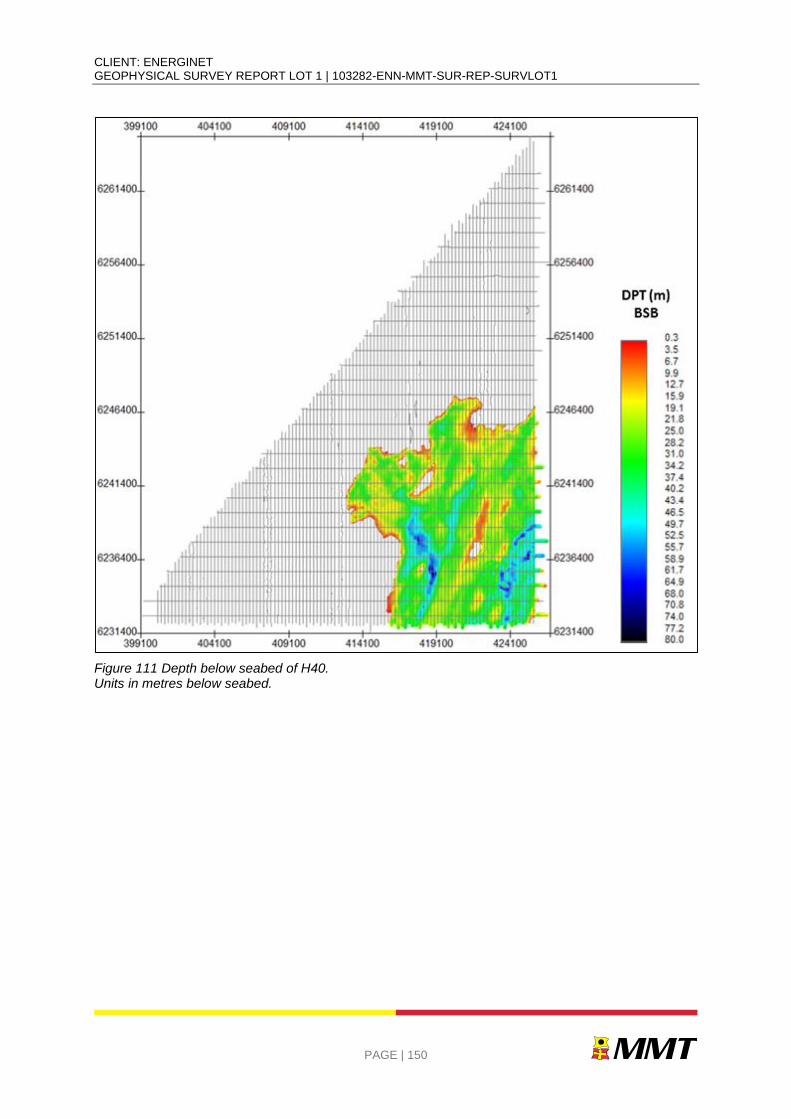
CLIENT: ENERGINET GEOPHYSICAL SURVEY REPORT LOT 1 | 103282-ENN-MMT-SUR-REP-SURVLOT1
PAGE | 150
Figure 111 Depth below seabed of H40. Units in metres below seabed.
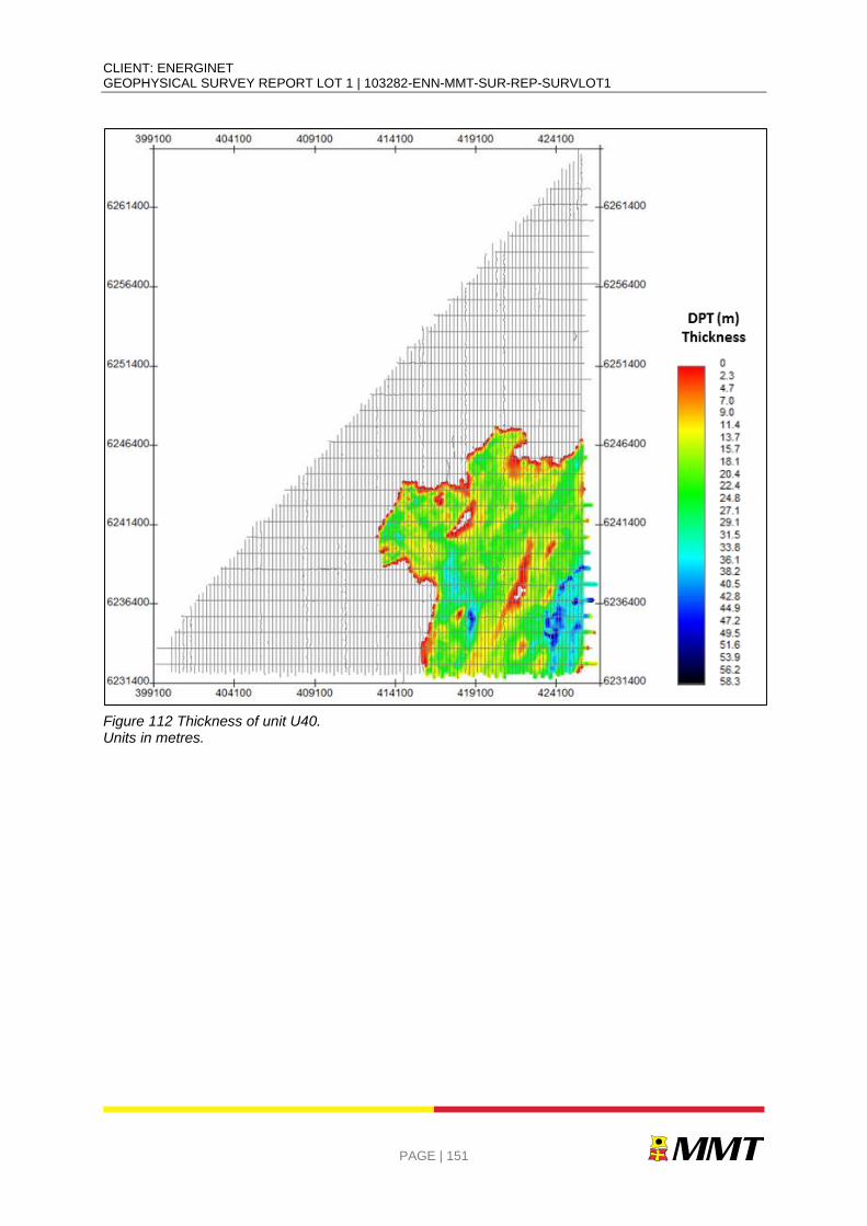
CLIENT: ENERGINET GEOPHYSICAL SURVEY REPORT LOT 1 | 103282-ENN-MMT-SUR-REP-SURVLOT1
PAGE | 151
Figure 112 Thickness of unit U40. Units in metres.
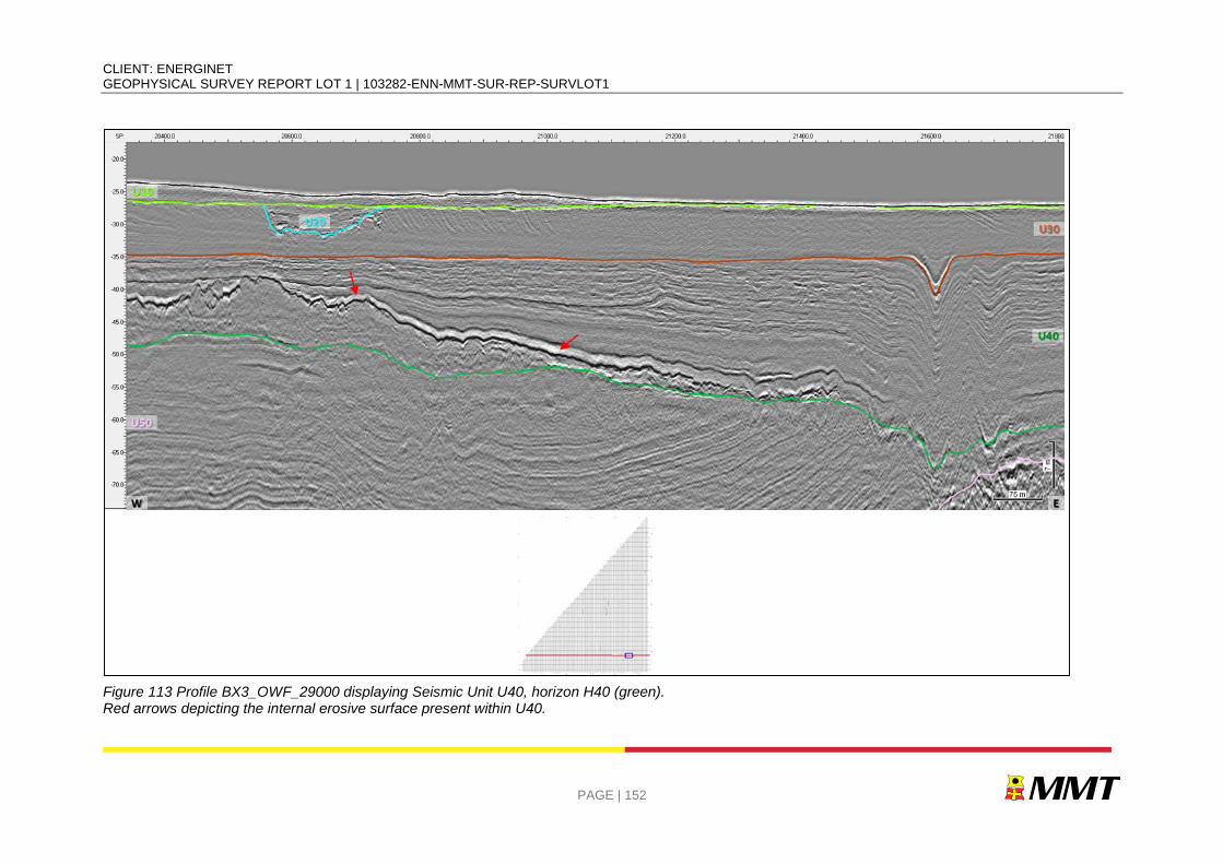
CLIENT: ENERGINET GEOPHYSICAL SURVEY REPORT LOT 1 | 103282-ENN-MMT-SUR-REP-SURVLOT1
PAGE | 152
Figure 113 Profile BX3_OWF_29000 displaying Seismic Unit U40, horizon H40 (green). Red arrows depicting the internal erosive surface present within U40.
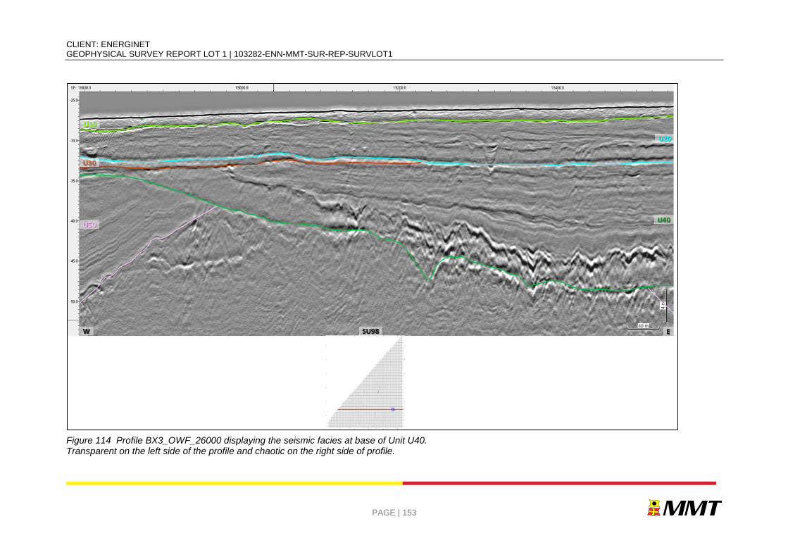
CLIENT: ENERGINET GEOPHYSICAL SURVEY REPORT LOT 1 | 103282-ENN-MMT-SUR-REP-SURVLOT1
PAGE | 153
Figure 114 Profile BX3_OWF_26000 displaying the seismic facies at base of Unit U40. Transparent on the left side of the profile and chaotic on the right side of profile.
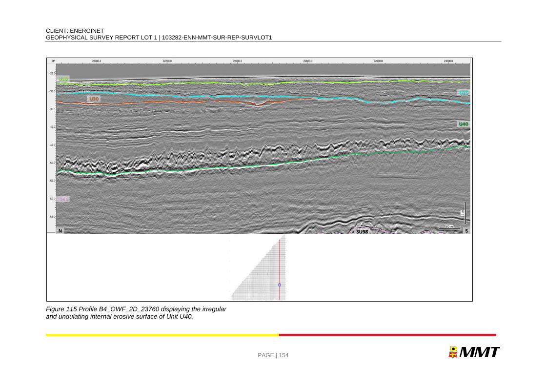
CLIENT: ENERGINET GEOPHYSICAL SURVEY REPORT LOT 1 | 103282-ENN-MMT-SUR-REP-SURVLOT1
PAGE | 154
Figure 115 Profile B4_OWF_2D_23760 displaying the irregular and undulating internal erosive surface of Unit U40.
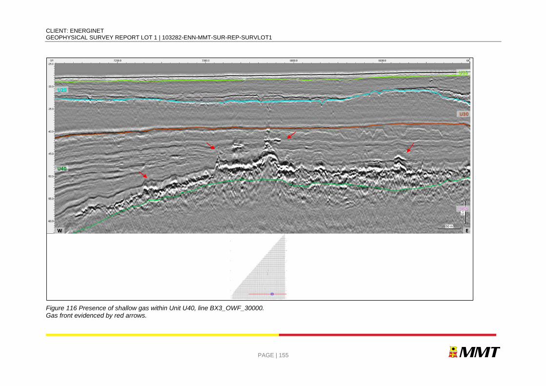
CLIENT: ENERGINET GEOPHYSICAL SURVEY REPORT LOT 1 | 103282-ENN-MMT-SUR-REP-SURVLOT1
PAGE | 155
Figure 116 Presence of shallow gas within Unit U40, line BX3_OWF_30000. Gas front evidenced by red arrows.
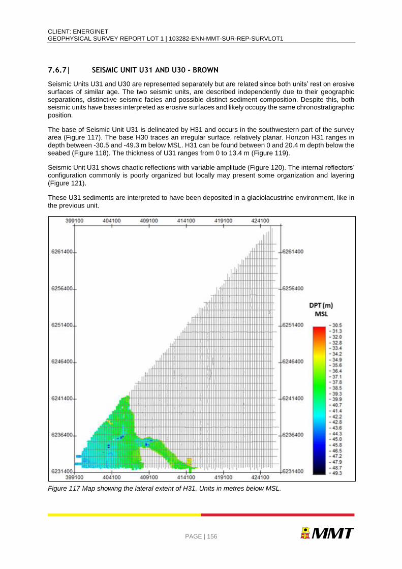
CLIENT: ENERGINET GEOPHYSICAL SURVEY REPORT LOT 1 | 103282-ENN-MMT-SUR-REP-SURVLOT1
PAGE | 156
7.6.7| SEISMIC UNIT U31 AND U30 – BROWN
Seismic Units U31 and U30 are represented separately but are related since both units’ rest on erosive surfaces of similar age. The two seismic units, are described independently due to their geographic separations, distinctive seismic facies and possible distinct sediment composition. Despite this, both seismic units have bases interpreted as erosive surfaces and likely occupy the same chronostratigraphic position.
The base of Seismic Unit U31 is delineated by H31 and occurs in the southwestern part of the survey area (Figure 117). The base H30 traces an irregular surface, relatively planar. Horizon H31 ranges in depth between -30.5 and -49.3 m below MSL. H31 can be found between 0 and 20.4 m depth below the seabed (Figure 118). The thickness of U31 ranges from 0 to 13.4 m (Figure 119).
Seismic Unit U31 shows chaotic reflections with variable amplitude (Figure 120). The internal reflectors’ configuration commonly is poorly organized but locally may present some organization and layering (Figure 121).
These U31 sediments are interpreted to have been deposited in a glaciolacustrine environment, like in the previous unit.
Figure 117 Map showing the lateral extent of H31. Units in metres below MSL.
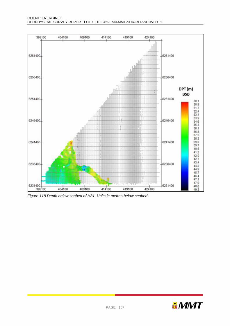
CLIENT: ENERGINET GEOPHYSICAL SURVEY REPORT LOT 1 | 103282-ENN-MMT-SUR-REP-SURVLOT1
PAGE | 157
Figure 118 Depth below seabed of H31. Units in metres below seabed.
CLIENT: ENERGINET GEOPHYSICAL SURVEY REPORT LOT 1 | 103282-ENN-MMT-SUR-REP-SURVLOT1
PAGE | 158
Figure 119 Thickness of unit U31. Units in metres.
CLIENT: ENERGINET GEOPHYSICAL SURVEY REPORT LOT 1 | 103282-ENN-MMT-SUR-REP-SURVLOT1
PAGE | 159
Figure 120 Profile B1_OWF_2D_6000 displaying chaotic reflections within seismic unit U31 horizon H31 (brown).
CLIENT: ENERGINET GEOPHYSICAL SURVEY REPORT LOT 1 | 103282-ENN-MMT-SUR-REP-SURVLOT1
PAGE | 160
Figure 121 Profile BX3_OWF_29000 displaying some organisation and layering within seismic unit U31.
CLIENT: ENERGINET GEOPHYSICAL SURVEY REPORT LOT 1 | 103282-ENN-MMT-SUR-REP-SURVLOT1
PAGE | 161
The base of Seismic Unit U30 is delineated by H30 and occurs in the southeastern part of the survey area (Figure 122). The base H30 traces a well-identifiable reflector with high amplitude contrast across the area. H30 displays undulating geometry, defining some depressions. Horizon H30 ranges in depth between 26.0 and 71.2 m below MSL. H30 can be found between 0 and 42.7 m depth below the seabed (Figure 123). The thickness of U30 ranges from 0 to 35.8 m (Figure 124).
U30 displays variable seismic facies (Figure 125 and Figure 126). The base of unit U40 shows sub-parallel, wavy and continuous reflections with moderate amplitude infilling some depressions/channels (Figure 125). The upper part of this unit displays transparent facies (Figure 126). Several downlap terminations are presented in the upper part of the unit, probably related to prograding sediments towards a basin/lake. These structures are represented by oblique configuration (Figure 127).
These sediments are interpreted to have been deposited in a glaciolacustrine environment, like the previous units (U40 and U31) with slightly different conditions. Presence of shallow gas within this unit is observed (Figure 128).
Figure 122 Map showing the lateral extent of H30. Units in metres below MSL.
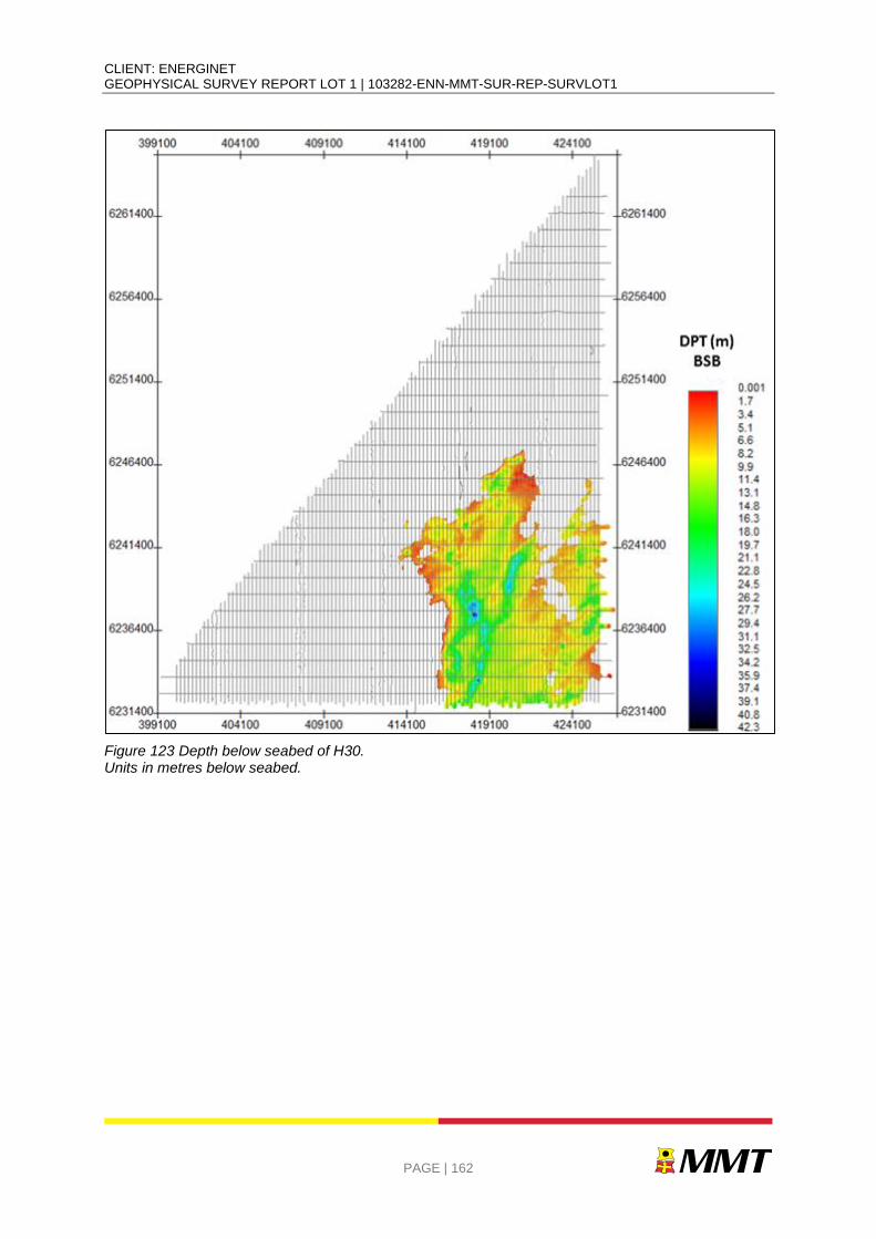
CLIENT: ENERGINET GEOPHYSICAL SURVEY REPORT LOT 1 | 103282-ENN-MMT-SUR-REP-SURVLOT1
PAGE | 162
Figure 123 Depth below seabed of H30. Units in metres below seabed.
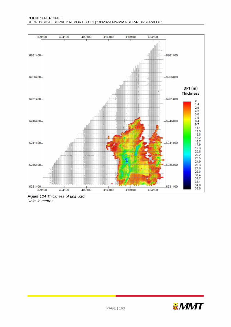
CLIENT: ENERGINET GEOPHYSICAL SURVEY REPORT LOT 1 | 103282-ENN-MMT-SUR-REP-SURVLOT1
PAGE | 163
Figure 124 Thickness of unit U30. Units in metres.
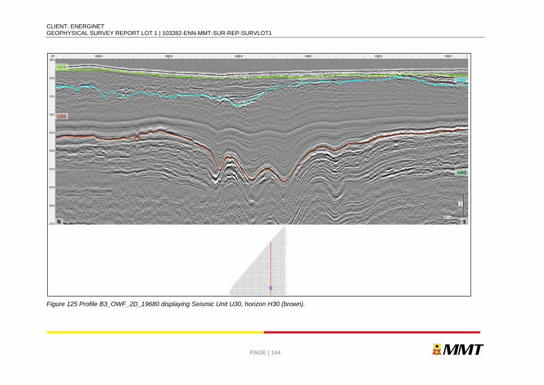
CLIENT: ENERGINET GEOPHYSICAL SURVEY REPORT LOT 1 | 103282-ENN-MMT-SUR-REP-SURVLOT1
PAGE | 164
Figure 125 Profile B3_OWF_2D_19680 displaying Seismic Unit U30, horizon H30 (brown).
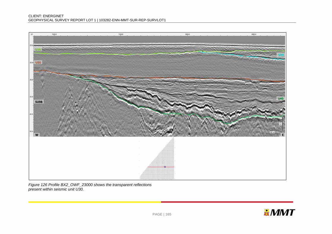
CLIENT: ENERGINET GEOPHYSICAL SURVEY REPORT LOT 1 | 103282-ENN-MMT-SUR-REP-SURVLOT1
PAGE | 165
Figure 126 Profile BX2_OWF_23000 shows the transparent reflections present within seismic unit U30.
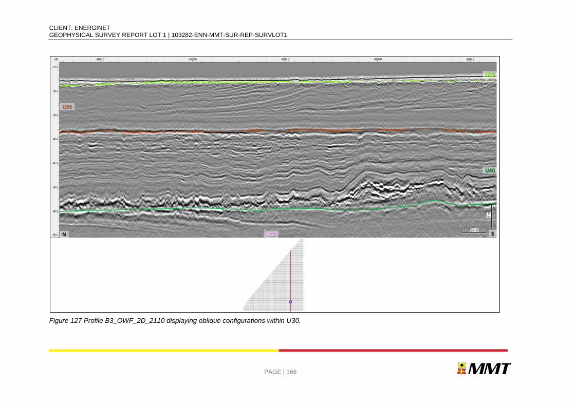
CLIENT: ENERGINET GEOPHYSICAL SURVEY REPORT LOT 1 | 103282-ENN-MMT-SUR-REP-SURVLOT1
PAGE | 166
Figure 127 Profile B3_OWF_2D_2110 displaying oblique configurations within U30.

CLIENT: ENERGINET GEOPHYSICAL SURVEY REPORT LOT 1 | 103282-ENN-MMT-SUR-REP-SURVLOT1
PAGE | 167
Figure 128 Presence of shallow gas within U30, line B3_OWF_2D_20400.
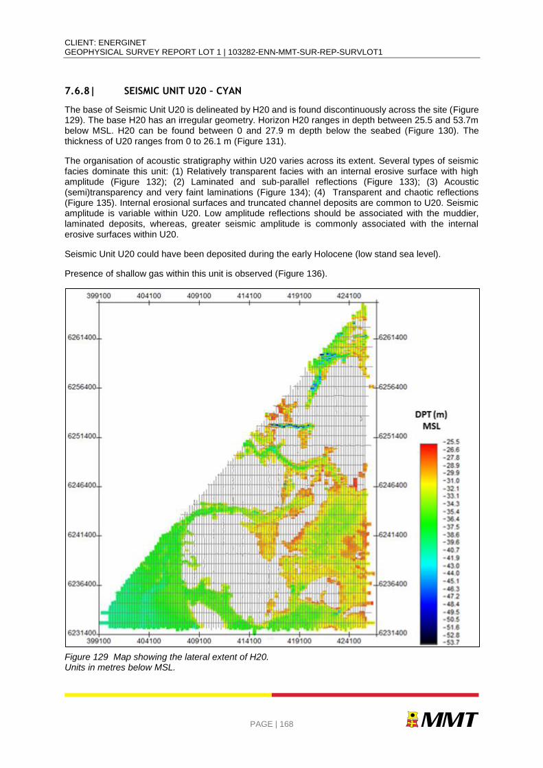
CLIENT: ENERGINET GEOPHYSICAL SURVEY REPORT LOT 1 | 103282-ENN-MMT-SUR-REP-SURVLOT1
PAGE | 168
7.6.8| SEISMIC UNIT U20 – CYAN
The base of Seismic Unit U20 is delineated by H20 and is found discontinuously across the site (Figure 129). The base H20 has an irregular geometry. Horizon H20 ranges in depth between 25.5 and 53.7m below MSL. H20 can be found between 0 and 27.9 m depth below the seabed (Figure 130). The thickness of U20 ranges from 0 to 26.1 m (Figure 131).
The organisation of acoustic stratigraphy within U20 varies across its extent. Several types of seismic facies dominate this unit: (1) Relatively transparent facies with an internal erosive surface with high amplitude (Figure 132); (2) Laminated and sub-parallel reflections (Figure 133); (3) Acoustic (semi)transparency and very faint laminations (Figure 134); (4) Transparent and chaotic reflections (Figure 135). Internal erosional surfaces and truncated channel deposits are common to U20. Seismic amplitude is variable within U20. Low amplitude reflections should be associated with the muddier, laminated deposits, whereas, greater seismic amplitude is commonly associated with the internal erosive surfaces within U20.
Seismic Unit U20 could have been deposited during the early Holocene (low stand sea level).
Presence of shallow gas within this unit is observed (Figure 136).
Figure 129 Map showing the lateral extent of H20. Units in metres below MSL.
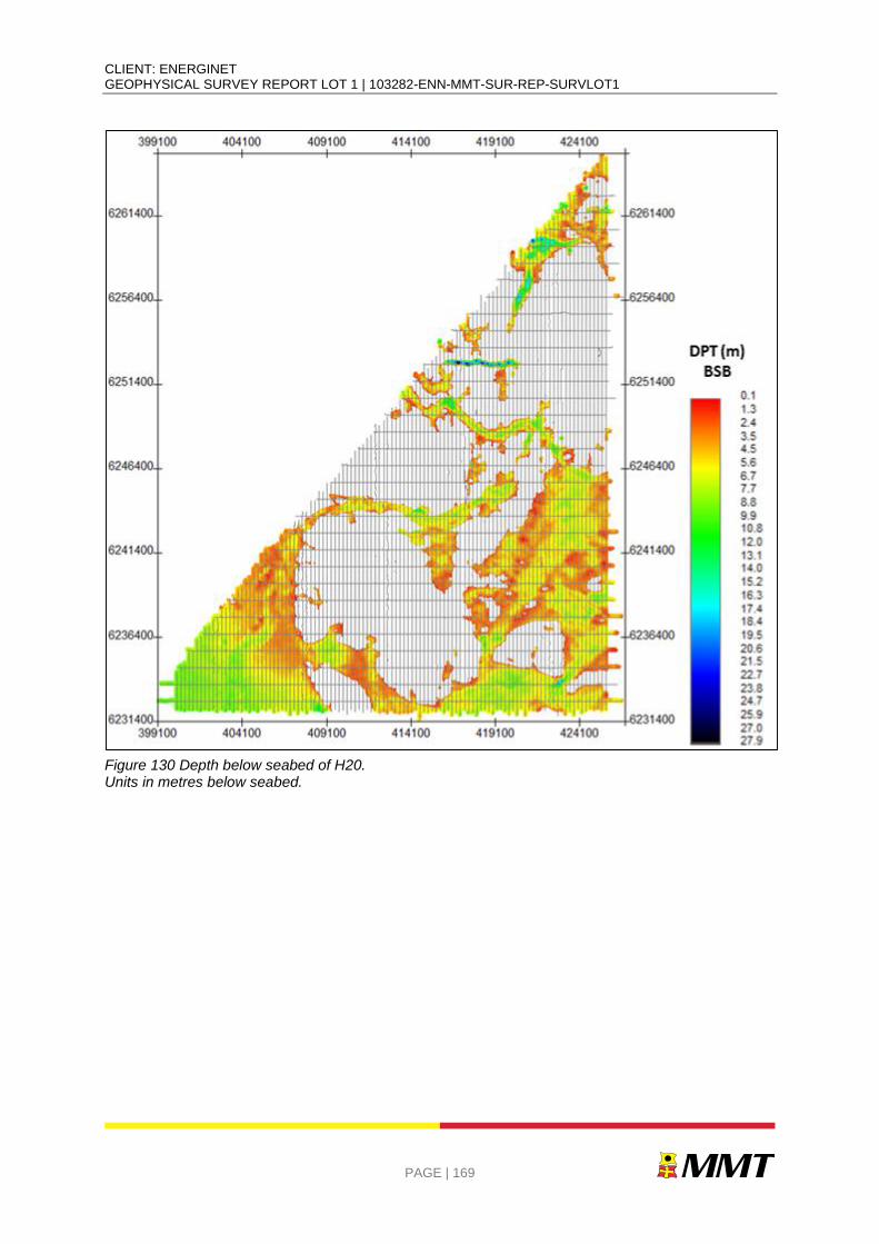
CLIENT: ENERGINET GEOPHYSICAL SURVEY REPORT LOT 1 | 103282-ENN-MMT-SUR-REP-SURVLOT1
PAGE | 169
Figure 130 Depth below seabed of H20. Units in metres below seabed.
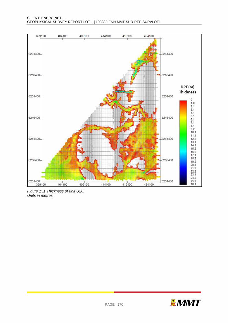
CLIENT: ENERGINET GEOPHYSICAL SURVEY REPORT LOT 1 | 103282-ENN-MMT-SUR-REP-SURVLOT1
PAGE | 170
Figure 131 Thickness of unit U20. Units in metres.
CLIENT: ENERGINET GEOPHYSICAL SURVEY REPORT LOT 1 | 103282-ENN-MMT-SUR-REP-SURVLOT1
PAGE | 171
Figure 132 Profile B4_OWF_2D_23520 displaying transparent facies within Unit U20, horizon H20 (light blue).
CLIENT: ENERGINET GEOPHYSICAL SURVEY REPORT LOT 1 | 103282-ENN-MMT-SUR-REP-SURVLOT1
PAGE | 172
Figure 133 Profile BX3_OWF_29000 displaying sub-parallel layering within Unit U20.
CLIENT: ENERGINET GEOPHYSICAL SURVEY REPORT LOT 1 | 103282-ENN-MMT-SUR-REP-SURVLOT1
PAGE | 173
Figure 134 Profile BX3_OWF_27000 displaying acoustic (semi)transparency and very faint laminations filling the channels/depressions present within Unit U20.
CLIENT: ENERGINET GEOPHYSICAL SURVEY REPORT LOT 1 | 103282-ENN-MMT-SUR-REP-SURVLOT1
PAGE | 174
Figure 135 Profile BX1_OWF_12000 shows transparent and chaotic reflections of Unit U20.
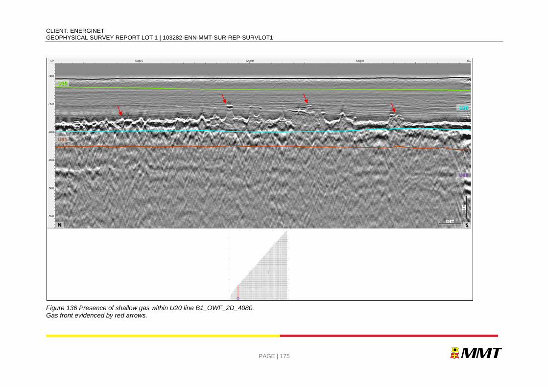
CLIENT: ENERGINET GEOPHYSICAL SURVEY REPORT LOT 1 | 103282-ENN-MMT-SUR-REP-SURVLOT1
PAGE | 175
Figure 136 Presence of shallow gas within U20 line B1_OWF_2D_4080. Gas front evidenced by red arrows.
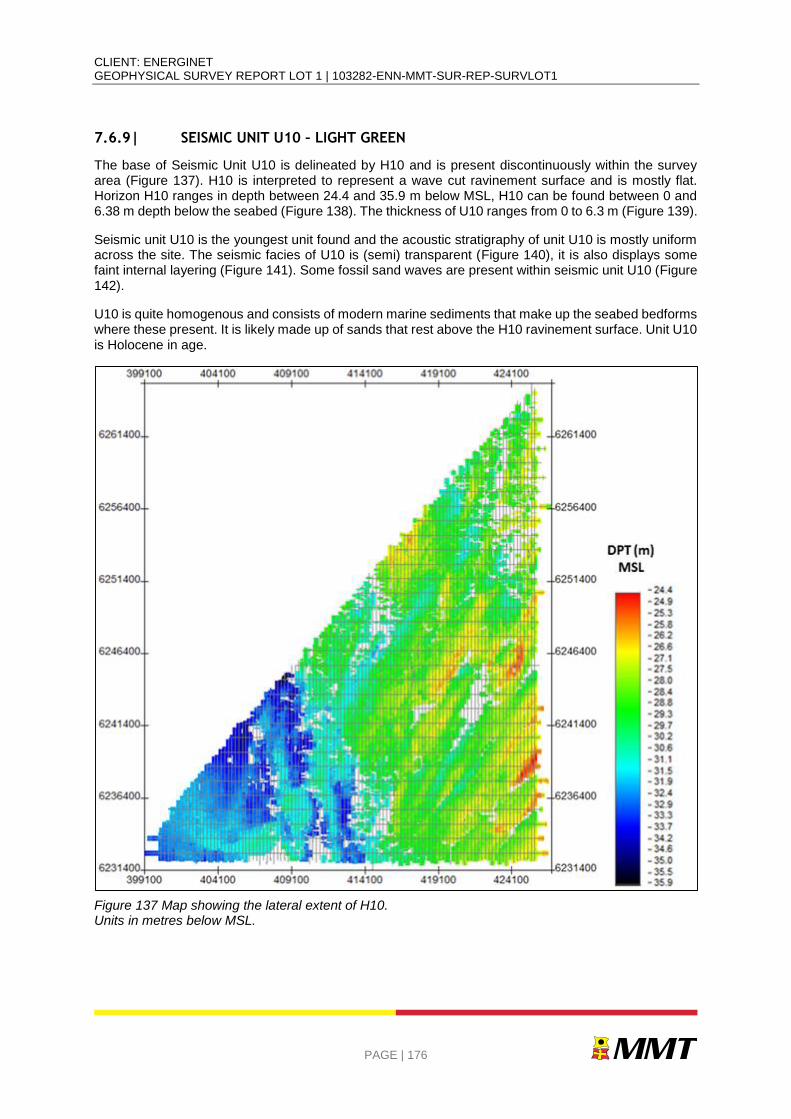
CLIENT: ENERGINET GEOPHYSICAL SURVEY REPORT LOT 1 | 103282-ENN-MMT-SUR-REP-SURVLOT1
PAGE | 176
7.6.9| SEISMIC UNIT U10 – LIGHT GREEN
The base of Seismic Unit U10 is delineated by H10 and is present discontinuously within the survey area (Figure 137). H10 is interpreted to represent a wave cut ravinement surface and is mostly flat. Horizon H10 ranges in depth between 24.4 and 35.9 m below MSL, H10 can be found between 0 and 6.38 m depth below the seabed (Figure 138). The thickness of U10 ranges from 0 to 6.3 m (Figure 139).
Seismic unit U10 is the youngest unit found and the acoustic stratigraphy of unit U10 is mostly uniform across the site. The seismic facies of U10 is (semi) transparent (Figure 140), it is also displays some faint internal layering (Figure 141). Some fossil sand waves are present within seismic unit U10 (Figure 142).
U10 is quite homogenous and consists of modern marine sediments that make up the seabed bedforms where these present. It is likely made up of sands that rest above the H10 ravinement surface. Unit U10 is Holocene in age.
Figure 137 Map showing the lateral extent of H10. Units in metres below MSL.
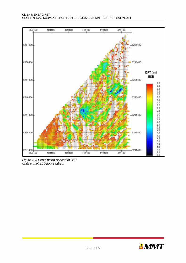
CLIENT: ENERGINET GEOPHYSICAL SURVEY REPORT LOT 1 | 103282-ENN-MMT-SUR-REP-SURVLOT1
PAGE | 177
Figure 138 Depth below seabed of H10. Units in metres below seabed.
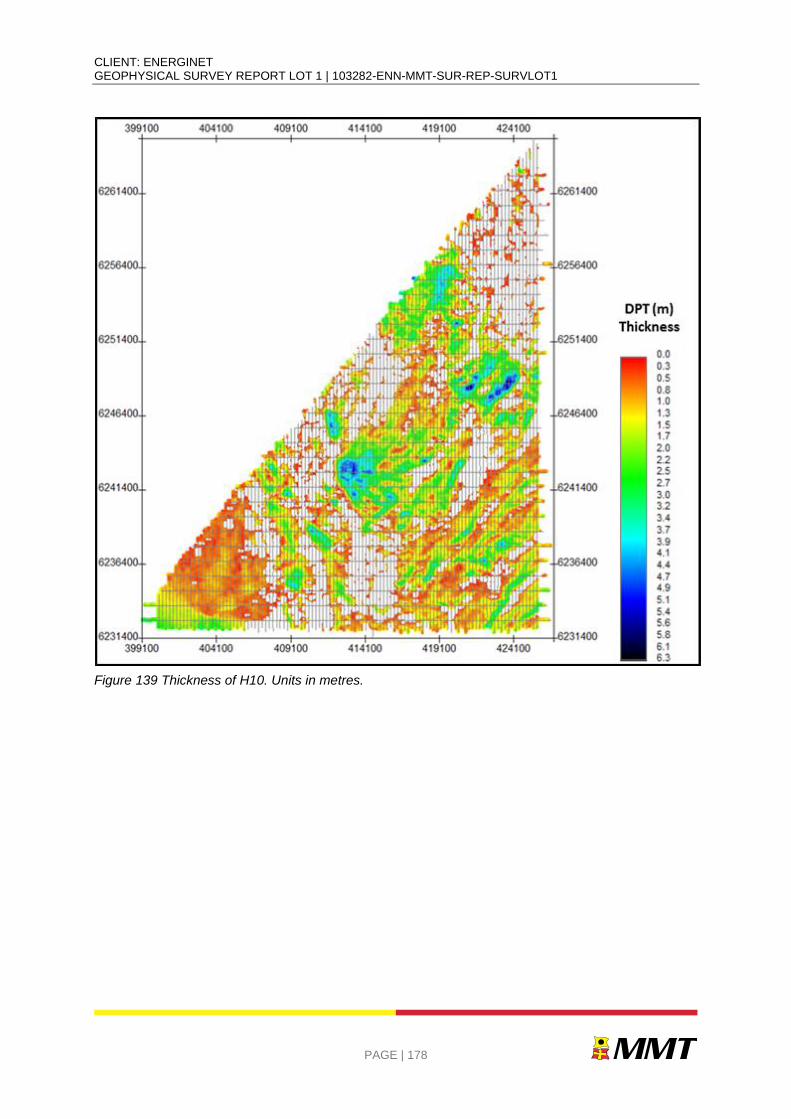
CLIENT: ENERGINET GEOPHYSICAL SURVEY REPORT LOT 1 | 103282-ENN-MMT-SUR-REP-SURVLOT1
PAGE | 178
Figure 139 Thickness of H10. Units in metres.
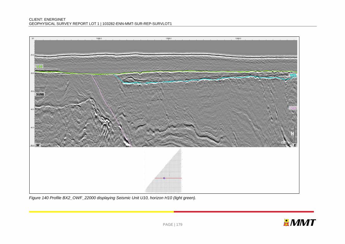
CLIENT: ENERGINET GEOPHYSICAL SURVEY REPORT LOT 1 | 103282-ENN-MMT-SUR-REP-SURVLOT1
PAGE | 179
Figure 140 Profile BX2_OWF_22000 displaying Seismic Unit U10, horizon H10 (light green).

CLIENT: ENERGINET GEOPHYSICAL SURVEY REPORT LOT 1 | 103282-ENN-MMT-SUR-REP-SURVLOT1
PAGE | 180
Figure 141 Profile B4_OWF_2D_24480 displaying some faint internal layering at the base of unit U10.
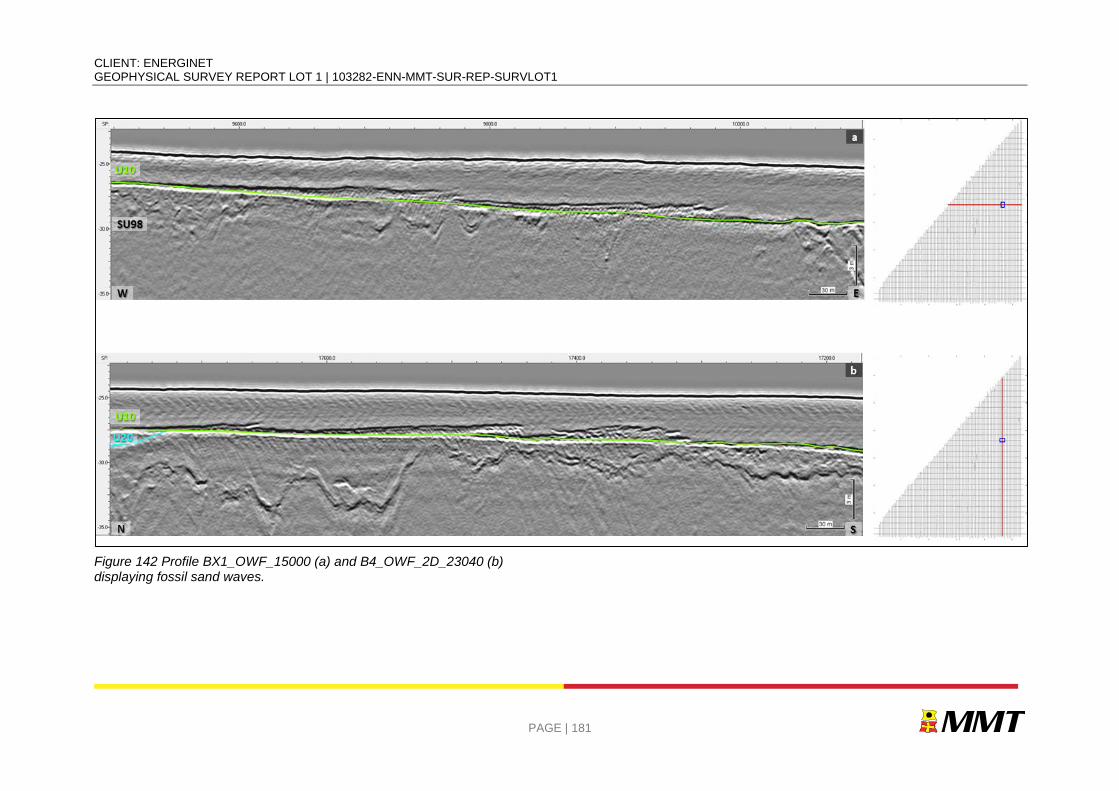
CLIENT: ENERGINET GEOPHYSICAL SURVEY REPORT LOT 1 | 103282-ENN-MMT-SUR-REP-SURVLOT1
PAGE | 181
Figure 142 Profile BX1_OWF_15000 (a) and B4_OWF_2D_23040 (b) displaying fossil sand waves.
CLIENT: ENERGINET GEOPHYSICAL SURVEY REPORT LOT 1 | 103282-ENN-MMT-SUR-REP-SURVLOT1
PAGE | 182
7.6.10| SUMMARY AND DISCUSSION
It is important that the user of this report understands the limitations of the interpretation provided. The inferred depositional environments and lithology descriptions contained in this report are based largely on seismic interpretation techniques. Seismic facies analysis, reflector terminations and stratigraphic architecture provided the foundation of the interpretation. A review of the relevant scientific literature provided a guide for the interpretation process and placed our results within a known geologic framework.
Seven horizons, all corresponding to units’ bases, are here proposed to make up the basis of this Geomodel. It takes into consideration the geometry of erosive surfaces depicted in the seismic profiles and the variability of seismic facies between different sedimentary packages. One other horizon was added to the Geomodel, mapped in order to separate two subunits within the base seismic unit. The seabed and processing last knee make up the top and lower boundaries of the Geomodel.
The uppermost unit (U10) is present at the seabed; overlying the remaining units (U20 to U50). U20 consist of infills of depressions and/or channels, which could be related to a lagoon system and partially a subaerial fluvial infill of a low stand erosive surface (sequence boundary). U30 and U31 have strata distinctive negative acoustic impedance contrasts at its base and could be correlated to a glaciolacustrine system. U40 is likely associated with a glaciolacustrine or a similar relatively low-energy environment. U45 could be related to a fluviodeltaic system in a moderate energy environment. U50 consists of fine layered sediments of glaciolacustrine origin and distinct laminated facies on the seismic profiles. The lowermost base unit, subdivided into SU98 and SU99 by T99, is a composite seismic unit comprising deformed sediments, which could be caused by glacial tectonics, valley infills and undeformed subparallel deltaic deposits (Miocene). Units’ bases are erosive in nature; still minor internal erosive surfaces also occur within the units.
7.7| SEABED HAZARDS
7.7.1| GRADIENTS
Slope angles across the site are typically very gentle (<1°) and gentle (1° to 5°). Despite the fact that sand wave areas constitute approximately 78% of the site the seafloor topography is typically gently undulating. Areas of moderate to very steep slopes are largely restricted to the edges of sand bodies and the lee slopes of the most defined sand waves.
Very steep slope angles (15° to a maximum of 43°) are associated with boulders, the edges of depressions and step-like features possibly associated with slumping of sediments and succeeding sediment movement. Slope angles up to 75° were observed, but were associated with boulder-like features identified within Deep Helder data that could not be disproved as system noise.
7.7.2| MOBILE SEDIMENT AND BEDFORMS
Mobile sediments are present throughout most of the surveyed area. They are most prominent in the central and northern parts. The mobile sediments comprise sand waves as well as megaripples and ripples. Areas of depressions and mass transport deposits found in conjunction to the sand waves are also believed to be caused by moving sediments.
CLIENT: ENERGINET GEOPHYSICAL SURVEY REPORT LOT 1 | 103282-ENN-MMT-SUR-REP-SURVLOT1
PAGE | 183
7.7.3| BOULDERS
Boulders are seen scattered throughout the site, most commonly occurring in the northern and central parts of the survey area.
7.7.4| EXISTING INFRASTUCTURE AND WRECKS
No pipelines or cables are present within Lot 1.
Two wrecks were detected during the survey correlating with the background information. Wreck S_DH_B01_0199 (400110c_134) was found at 411116 m E, 6242717 m N and wreck S_DH_B03_0559, M_103 (400110c-132) was found at 421836 m E, 6242042 m N.
7.8| SUB-SEABED HAZARDS
The inspection of the seismic datasets was done in order to identify any potential constrain on future development of the site; it does not directly correlate with a real risk. Inspection of 2D UHRS seismic data for the reference lines revealed the presence of potential geohazards; the most relevant of these are:
Tectonized sediments;
Faulting;
Paleo-valley infill sediments;
Organic-rich deposits;
Coarse sediments/Gravel Layers;
Shallow gas.
The interpretation and mapping of all hazards present in this section were performed using manual picking as seismic data resolution and human precision allowed.
A more detailed description of the aforementioned geological hazards is presented within Sections 7.8.1| to 7.8.6| below.
7.8.1| TECTONIZED SEDIMENTS
Areas of tectonization/deformation were identified within the seismic subunit SU98. The origin of these deformed deposits is interpreted to be glacial tectonics. Internal reflections typically appear wavy and folded, but may be chaotic, displaying complete incoherence (Figure 143). Depending on the angle where the seismic profile crosses the tectonized sediments, these units may appear (semi) acoustically transparent. In many cases the sediment within these units has been deformed to the point where internal stratification is uninterpretable. However, in some instances, the original stratigraphy of the unit may be preserved to some extent, Figure 144. The sediments comprising the tectonized units have been substantially disturbed from their original depositional attitude. The materials within these units are likely to have experienced variable and complex stress, i.e., compressional, tensional, and shear (Figure 145). These units should have geotechnical significance given their complex stress/load histories.
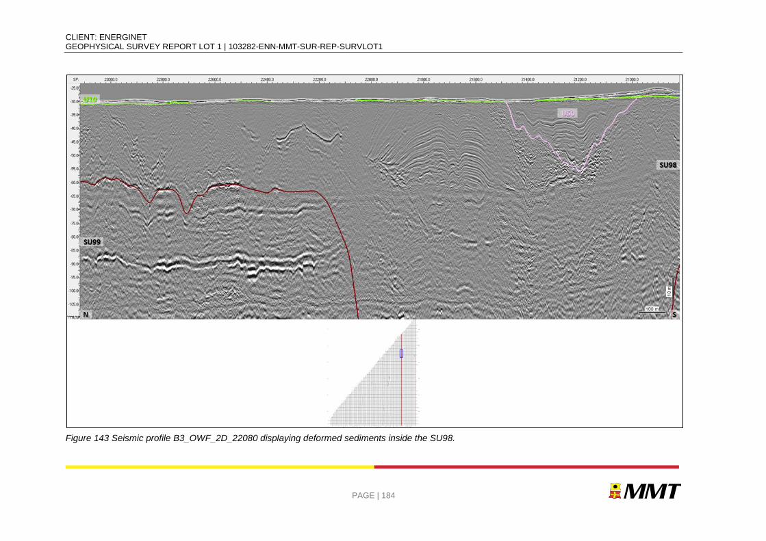
CLIENT: ENERGINET GEOPHYSICAL SURVEY REPORT LOT 1 | 103282-ENN-MMT-SUR-REP-SURVLOT1
PAGE | 184
Figure 143 Seismic profile B3_OWF_2D_22080 displaying deformed sediments inside the SU98.
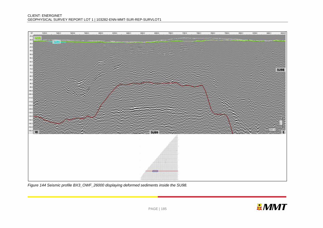
CLIENT: ENERGINET GEOPHYSICAL SURVEY REPORT LOT 1 | 103282-ENN-MMT-SUR-REP-SURVLOT1
PAGE | 185
Figure 144 Seismic profile BX3_OWF_26000 displaying deformed sediments inside the SU98.
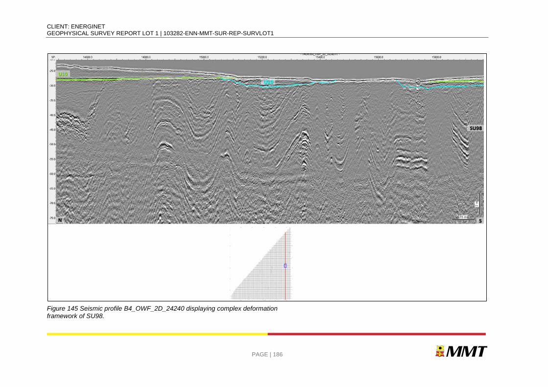
CLIENT: ENERGINET GEOPHYSICAL SURVEY REPORT LOT 1 | 103282-ENN-MMT-SUR-REP-SURVLOT1
PAGE | 186
Figure 145 Seismic profile B4_OWF_2D_24240 displaying complex deformation framework of SU98.
CLIENT: ENERGINET GEOPHYSICAL SURVEY REPORT LOT 1 | 103282-ENN-MMT-SUR-REP-SURVLOT1
PAGE | 187
7.8.2| FAULTING
Presence of faults can represent a general risk to construction and engineering operations. Evidence of faulting has been identified across the site with limited spatial extension. Faults were picked manually where relevant planar discontinuities, displacement of seismic reflectors and major reflector-fault drags were recognized on the seismic data. Depending on the angle between the faults and the seismic sections, some features may appear more noticeable than others. A way to mitigate this was by inspecting the fault basemap to ensure that features were digitized on a coherent and continuous manner; i.e., tracing was done from lines where the faults were more evident to lines with reduced expression. Figure 146 displays the final fault basemap produced. Minor, isolated and dubious features may have been left out due to the complexity of the subsurface framework and difficulty in recognizing all features and faults.
Faults are present in some units and do not greatly affect sediments younger than U30 (Figure 147). However, this lack of identification should not be taken as an assumption of total absence.
Faults were identified within units U40 (Figure 147) and U50 (Figure 148). Subunits SU98 (Figure 149) and SU99 (Figure 150) also display several features affecting and displacing the sediments.
The presence of faults in this site could be related with the presence of the ice sheet during the Elsterian and Saalian glaciations. Faults affecting the deeper deposits of SU99 are probably related with diapirism well known to occur in the area (Zechstein salt tectonism, e.g. Michelsen 1993).
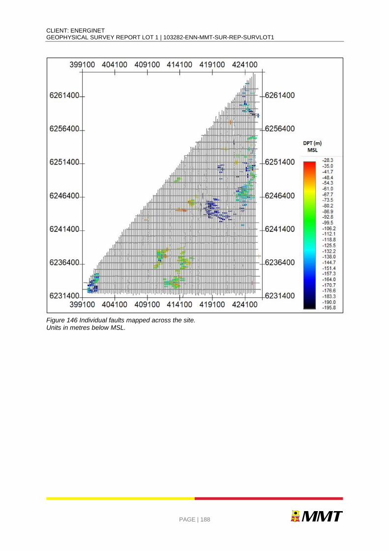
CLIENT: ENERGINET GEOPHYSICAL SURVEY REPORT LOT 1 | 103282-ENN-MMT-SUR-REP-SURVLOT1
PAGE | 188
Figure 146 Individual faults mapped across the site. Units in metres below MSL.
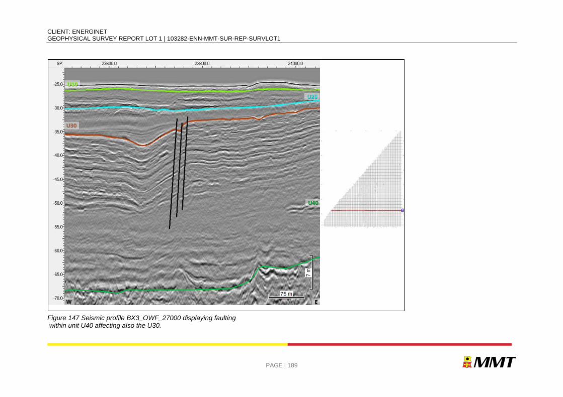
CLIENT: ENERGINET GEOPHYSICAL SURVEY REPORT LOT 1 | 103282-ENN-MMT-SUR-REP-SURVLOT1
PAGE | 189
Figure 147 Seismic profile BX3_OWF_27000 displaying faulting within unit U40 affecting also the U30.
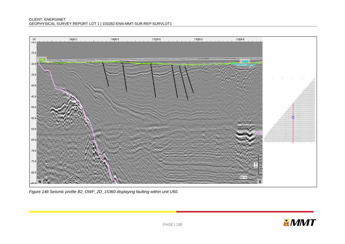
CLIENT: ENERGINET GEOPHYSICAL SURVEY REPORT LOT 1 | 103282-ENN-MMT-SUR-REP-SURVLOT1
PAGE | 190
Figure 148 Seismic profile B2_OWF_2D_15360 displaying faulting within unit U50.
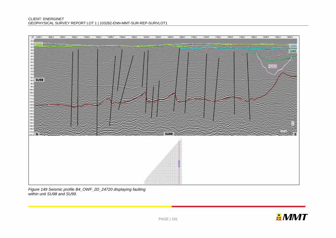
CLIENT: ENERGINET GEOPHYSICAL SURVEY REPORT LOT 1 | 103282-ENN-MMT-SUR-REP-SURVLOT1
PAGE | 191
Figure 149 Seismic profile B4_OWF_2D_24720 displaying faulting within unit SU98 and SU99.
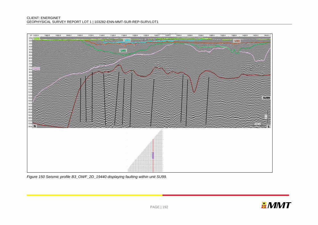
CLIENT: ENERGINET GEOPHYSICAL SURVEY REPORT LOT 1 | 103282-ENN-MMT-SUR-REP-SURVLOT1
PAGE | 192
Figure 150 Seismic profile B3_OWF_2D_19440 displaying faulting within unit SU99.
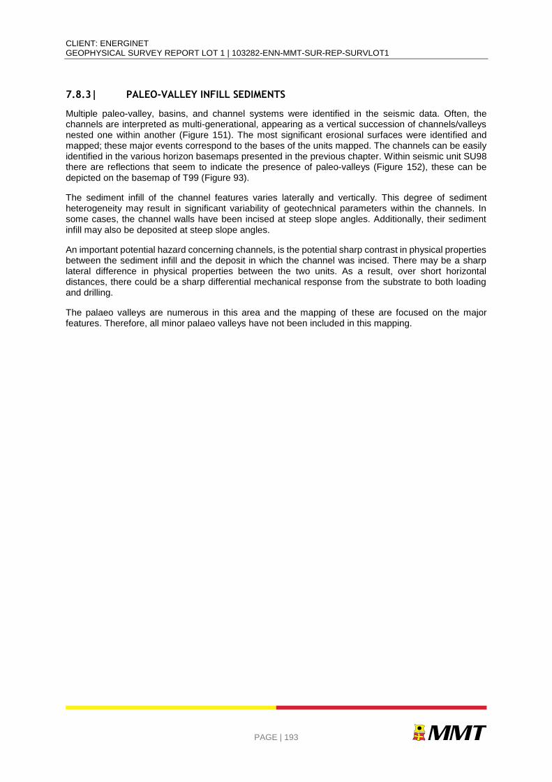
CLIENT: ENERGINET GEOPHYSICAL SURVEY REPORT LOT 1 | 103282-ENN-MMT-SUR-REP-SURVLOT1
PAGE | 193
7.8.3| PALEO-VALLEY INFILL SEDIMENTS
Multiple paleo-valley, basins, and channel systems were identified in the seismic data. Often, the channels are interpreted as multi-generational, appearing as a vertical succession of channels/valleys nested one within another (Figure 151). The most significant erosional surfaces were identified and mapped; these major events correspond to the bases of the units mapped. The channels can be easily identified in the various horizon basemaps presented in the previous chapter. Within seismic unit SU98 there are reflections that seem to indicate the presence of paleo-valleys (Figure 152), these can be depicted on the basemap of T99 (Figure 93).
The sediment infill of the channel features varies laterally and vertically. This degree of sediment heterogeneity may result in significant variability of geotechnical parameters within the channels. In some cases, the channel walls have been incised at steep slope angles. Additionally, their sediment infill may also be deposited at steep slope angles.
An important potential hazard concerning channels, is the potential sharp contrast in physical properties between the sediment infill and the deposit in which the channel was incised. There may be a sharp lateral difference in physical properties between the two units. As a result, over short horizontal distances, there could be a sharp differential mechanical response from the substrate to both loading and drilling.
The palaeo valleys are numerous in this area and the mapping of these are focused on the major features. Therefore, all minor palaeo valleys have not been included in this mapping.
CLIENT: ENERGINET GEOPHYSICAL SURVEY REPORT LOT 1 | 103282-ENN-MMT-SUR-REP-SURVLOT1
PAGE | 194
Figure 151 Profile BX3_OWF_27000 displaying the channel features in different seismic units.

CLIENT: ENERGINET GEOPHYSICAL SURVEY REPORT LOT 1 | 103282-ENN-MMT-SUR-REP-SURVLOT1
PAGE | 195
Figure 152 Profile B2_OWF_2D_12960 displaying paleo-valleys within SU98.
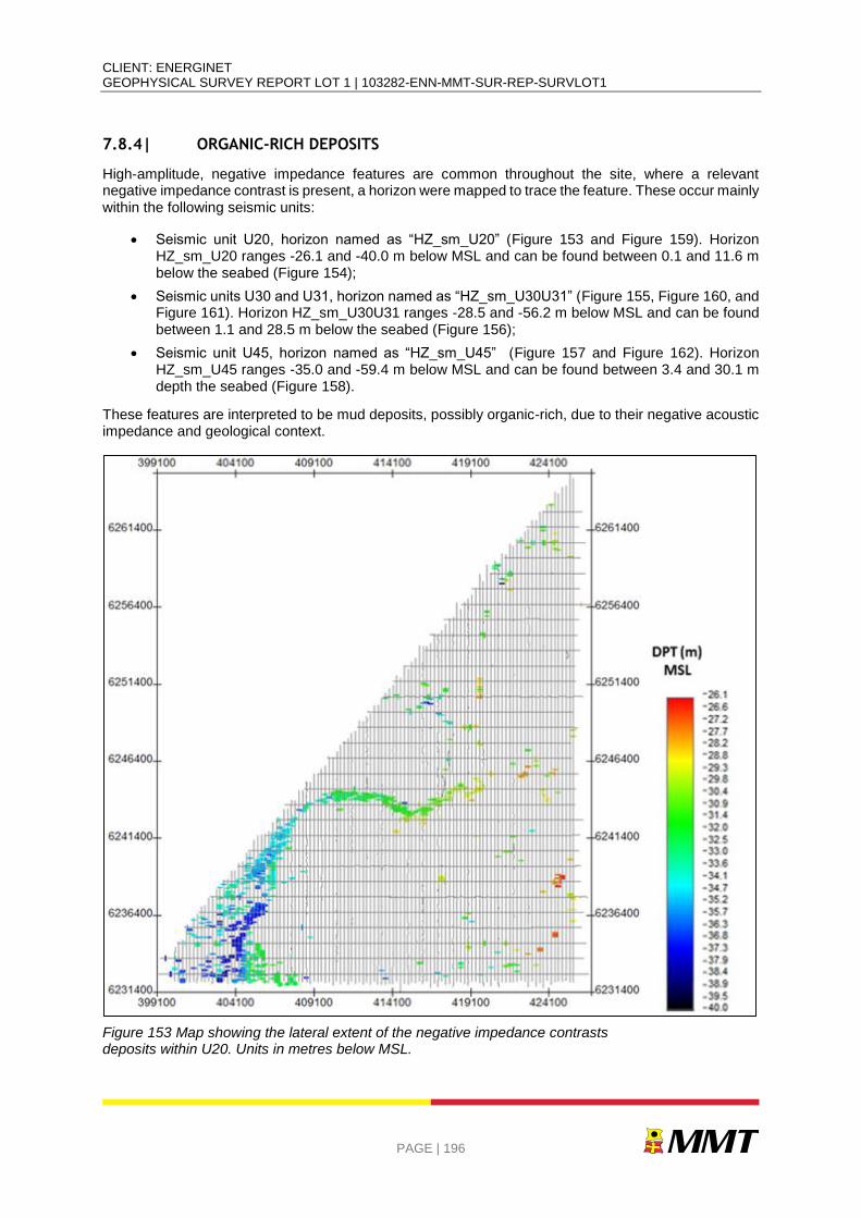
CLIENT: ENERGINET GEOPHYSICAL SURVEY REPORT LOT 1 | 103282-ENN-MMT-SUR-REP-SURVLOT1
PAGE | 196
7.8.4| ORGANIC-RICH DEPOSITS
High-amplitude, negative impedance features are common throughout the site, where a relevant negative impedance contrast is present, a horizon were mapped to trace the feature. These occur mainly within the following seismic units:
Seismic unit U20, horizon named as “HZ_sm_U20” (Figure 153 and Figure 159). Horizon HZ_sm_U20 ranges -26.1 and -40.0 m below MSL and can be found between 0.1 and 11.6 m below the seabed (Figure 154);
Seismic units U30 and U31, horizon named as “HZ_sm_U30U31” (Figure 155, Figure 160, and Figure 161). Horizon HZ_sm_U30U31 ranges -28.5 and -56.2 m below MSL and can be found between 1.1 and 28.5 m below the seabed (Figure 156);
Seismic unit U45, horizon named as “HZ_sm_U45” (Figure 157 and Figure 162). Horizon HZ_sm_U45 ranges -35.0 and -59.4 m below MSL and can be found between 3.4 and 30.1 m depth the seabed (Figure 158).
These features are interpreted to be mud deposits, possibly organic-rich, due to their negative acoustic impedance and geological context.
Figure 153 Map showing the lateral extent of the negative impedance contrasts deposits within U20. Units in metres below MSL.
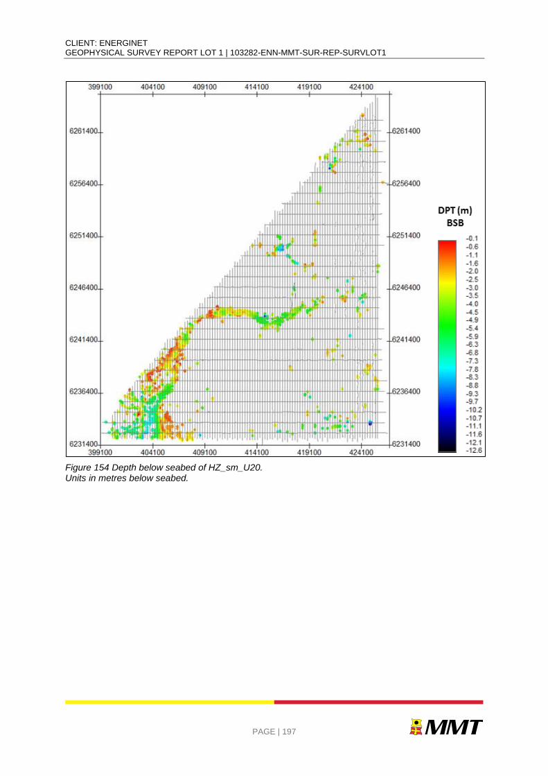
CLIENT: ENERGINET GEOPHYSICAL SURVEY REPORT LOT 1 | 103282-ENN-MMT-SUR-REP-SURVLOT1
PAGE | 197
Figure 154 Depth below seabed of HZ_sm_U20. Units in metres below seabed.
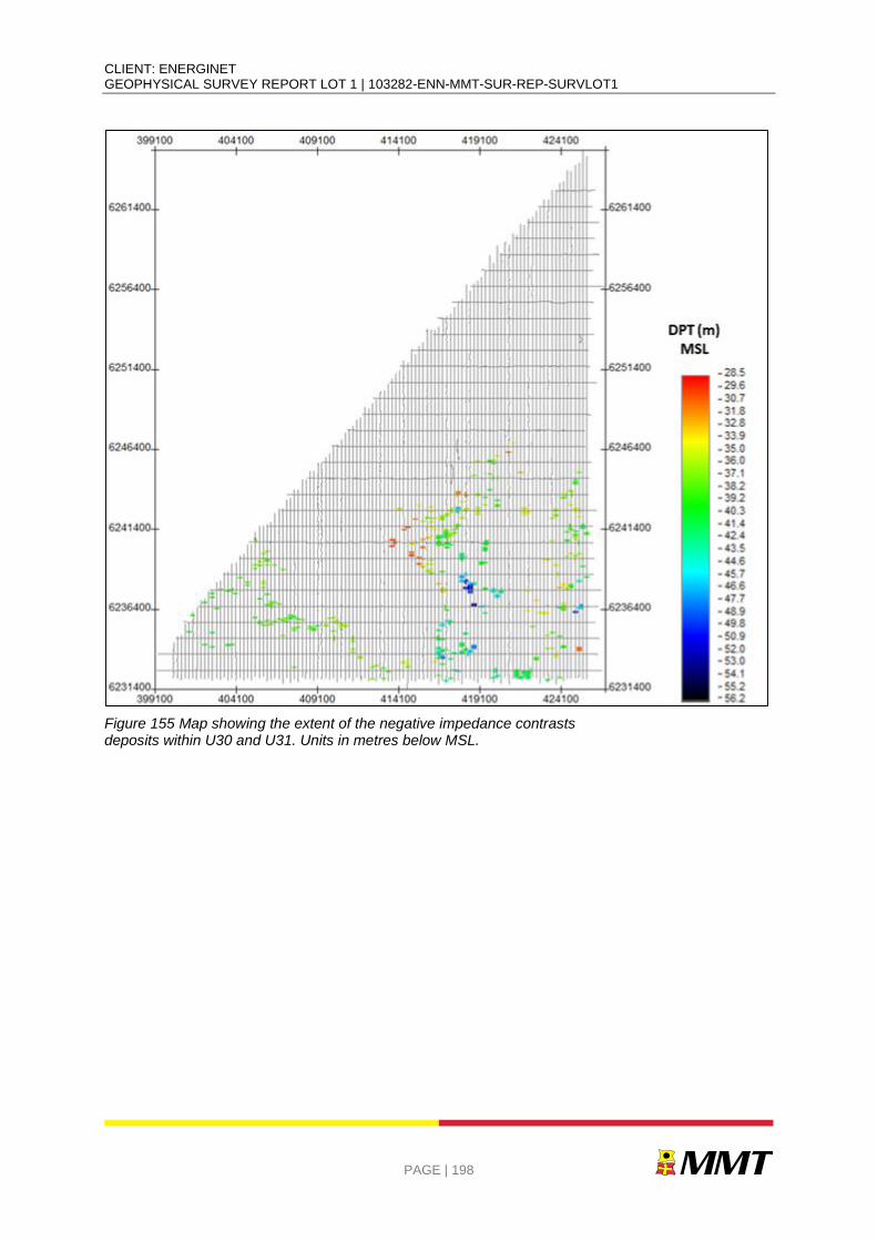
CLIENT: ENERGINET GEOPHYSICAL SURVEY REPORT LOT 1 | 103282-ENN-MMT-SUR-REP-SURVLOT1
PAGE | 198
Figure 155 Map showing the extent of the negative impedance contrasts deposits within U30 and U31. Units in metres below MSL.
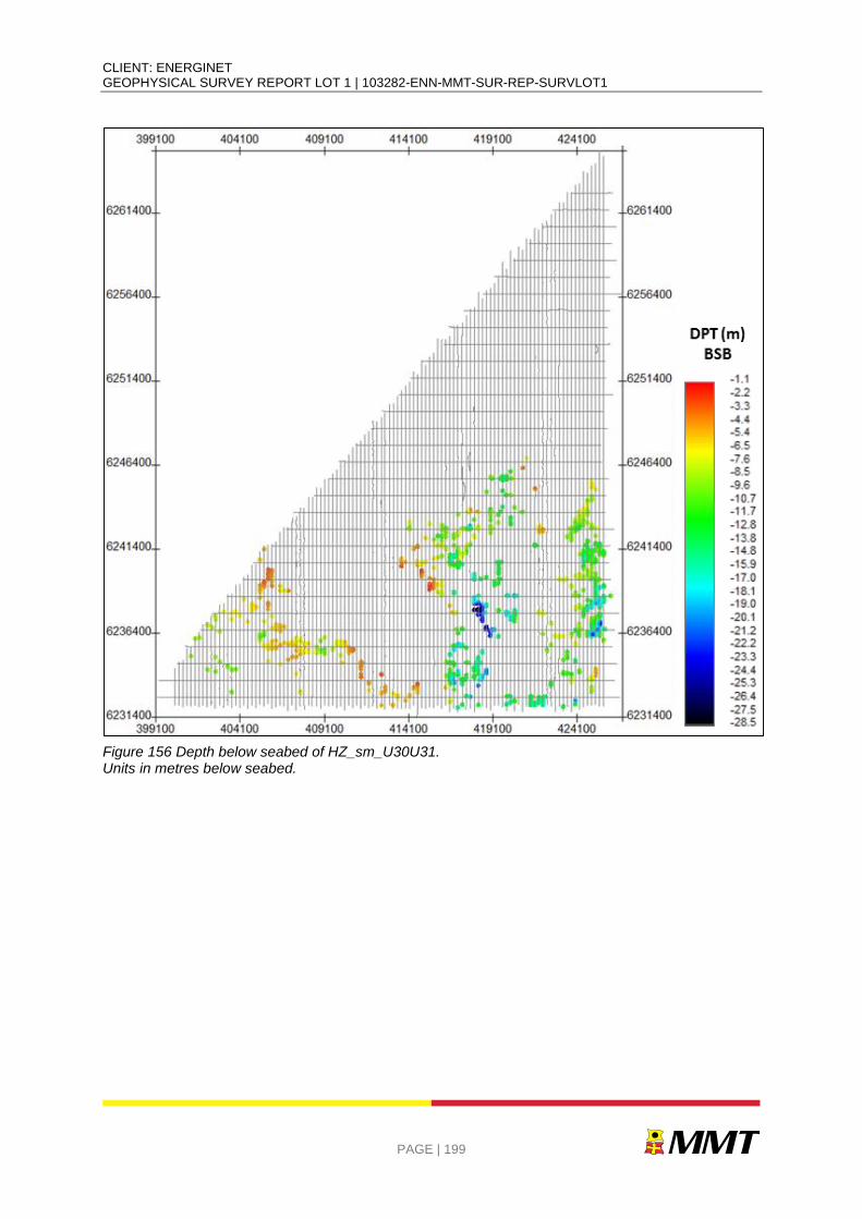
CLIENT: ENERGINET GEOPHYSICAL SURVEY REPORT LOT 1 | 103282-ENN-MMT-SUR-REP-SURVLOT1
PAGE | 199
Figure 156 Depth below seabed of HZ_sm_U30U31. Units in metres below seabed.
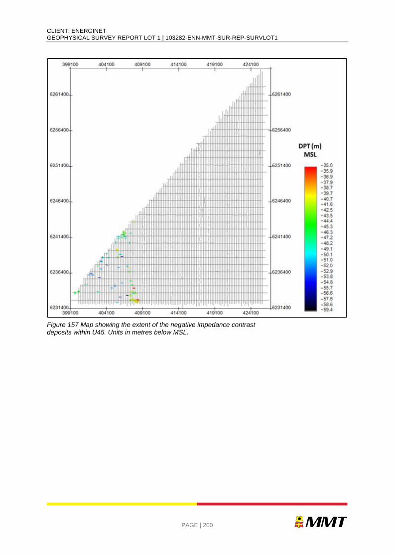
CLIENT: ENERGINET GEOPHYSICAL SURVEY REPORT LOT 1 | 103282-ENN-MMT-SUR-REP-SURVLOT1
PAGE | 200
Figure 157 Map showing the extent of the negative impedance contrast deposits within U45. Units in metres below MSL.
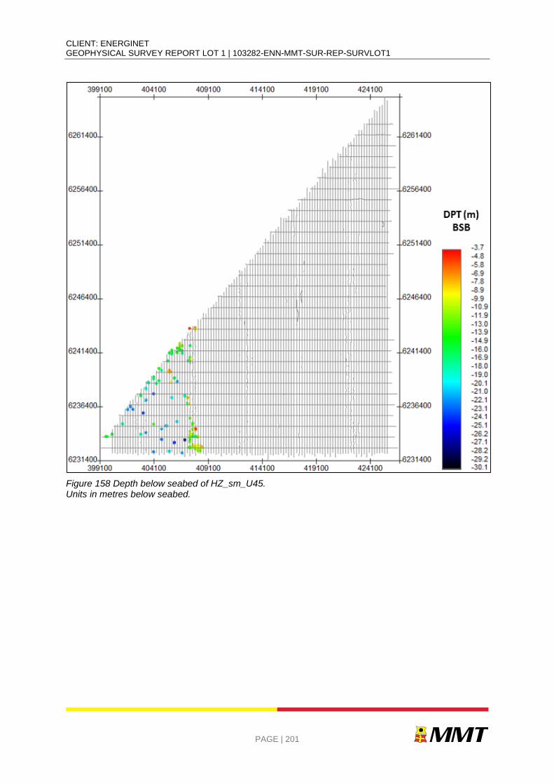
CLIENT: ENERGINET GEOPHYSICAL SURVEY REPORT LOT 1 | 103282-ENN-MMT-SUR-REP-SURVLOT1
PAGE | 201
Figure 158 Depth below seabed of HZ_sm_U45. Units in metres below seabed.
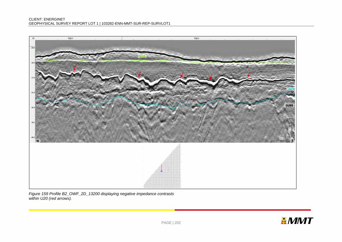
CLIENT: ENERGINET GEOPHYSICAL SURVEY REPORT LOT 1 | 103282-ENN-MMT-SUR-REP-SURVLOT1
PAGE | 202
Figure 159 Profile B2_OWF_2D_13200 displaying negative impedance contrasts within U20 (red arrows).
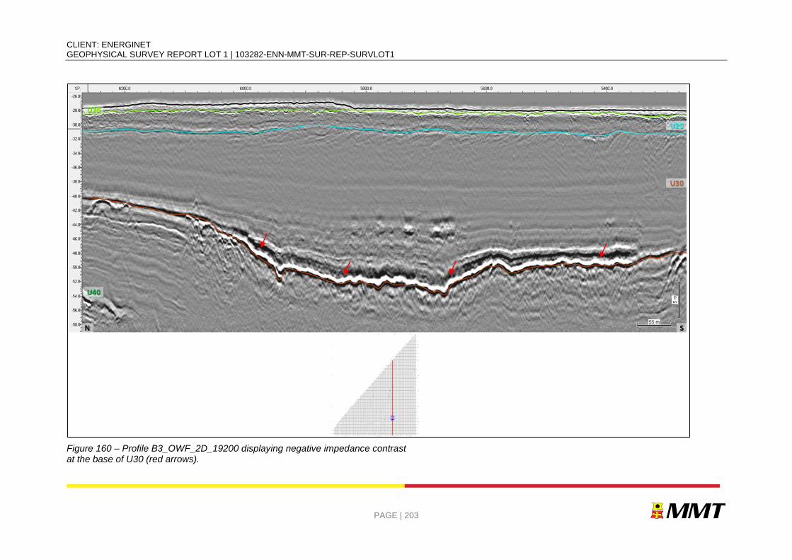
CLIENT: ENERGINET GEOPHYSICAL SURVEY REPORT LOT 1 | 103282-ENN-MMT-SUR-REP-SURVLOT1
PAGE | 203
Figure 160 – Profile B3_OWF_2D_19200 displaying negative impedance contrast at the base of U30 (red arrows).
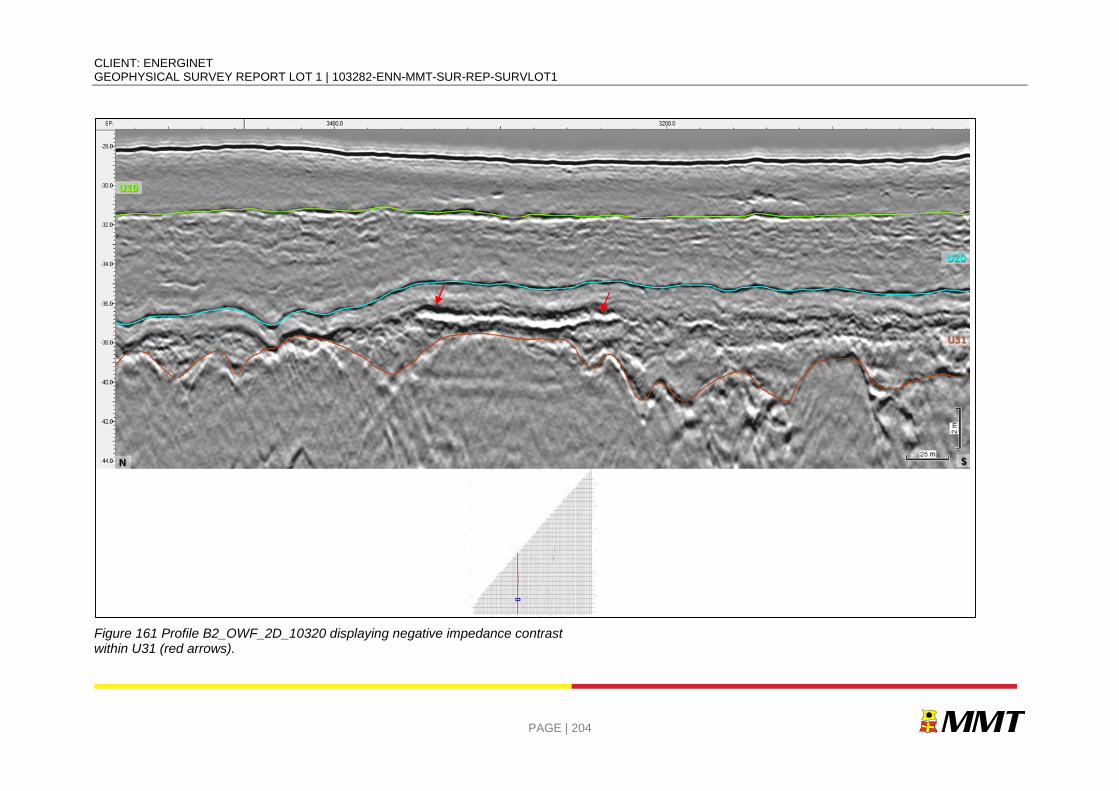
CLIENT: ENERGINET GEOPHYSICAL SURVEY REPORT LOT 1 | 103282-ENN-MMT-SUR-REP-SURVLOT1
PAGE | 204
Figure 161 Profile B2_OWF_2D_10320 displaying negative impedance contrast within U31 (red arrows).
CLIENT: ENERGINET GEOPHYSICAL SURVEY REPORT LOT 1 | 103282-ENN-MMT-SUR-REP-SURVLOT1
PAGE | 205
Figure 162 Profile BX3_OWF_3200 displaying negative impedance contrast within U45 (red arrows).
CLIENT: ENERGINET GEOPHYSICAL SURVEY REPORT LOT 1 | 103282-ENN-MMT-SUR-REP-SURVLOT1
PAGE | 206
7.8.5| COARSE SEDIMENTS/GRAVEL LAYERS
Coarser sediments like gravel lag and boulder accumulations are potential hazards and may constitute a constraint on drilling and other operations. Large gravel, cobbles and boulders may cause severe damage to equipment and affect infrastructure installation.
Coarser material, such as boulders, cobbles, gravel lags and ancient wood (logs) are present in glacial environments and associated seismic records. The immediate source of the large pebble, cobble and boulder size classes originates from older formations that have been submerged during rising sea level. However, point diffractors are not only related to boulder contacts. Acoustic signature and geological/seismostratigraphic context have to be taken into consideration when interpreting these types of reflections.
A coarse layer present in a restricted part of the site is displayed in Figure 163. The top of such feature was traced with horizon “HZ_01”. HZ_01 ranges -35.9 and -92.4 m below MSL and can be found between 3.0 and 65.4 m depth below the seabed (Figure 163, Figure 164). The coarse layer mapped is present within U45 (Figure 165) and SU99 representing the Miocene sediments (Figure 166).
Figure 163 Map showing the lateral extent of HZ_01. Units in metres below MSL.
CLIENT: ENERGINET GEOPHYSICAL SURVEY REPORT LOT 1 | 103282-ENN-MMT-SUR-REP-SURVLOT1
PAGE | 207
Figure 164 Depth below seabed of HZ_01. Units in metres below seabed.
CLIENT: ENERGINET GEOPHYSICAL SURVEY REPORT LOT 1 | 103282-ENN-MMT-SUR-REP-SURVLOT1
PAGE | 208
Figure 165 Profile BX3_OWF_32000 displaying a possible coarse layer within U45 (Red arrows indicates coarse material).
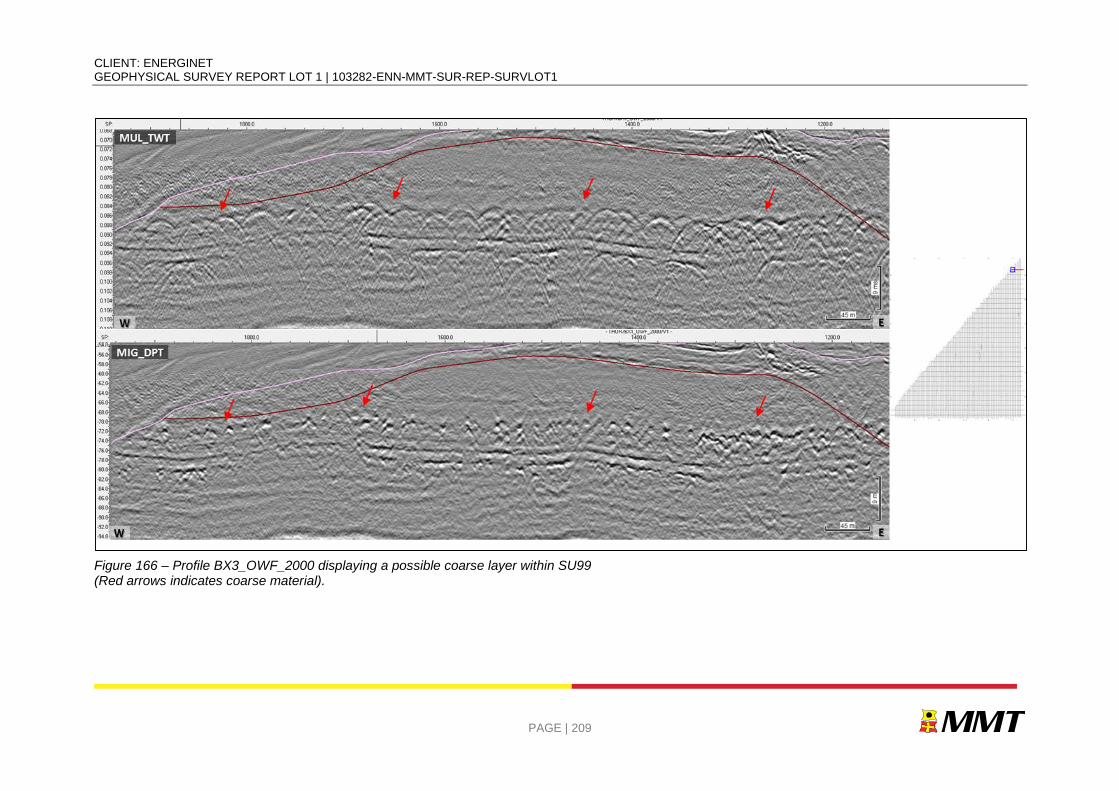
CLIENT: ENERGINET GEOPHYSICAL SURVEY REPORT LOT 1 | 103282-ENN-MMT-SUR-REP-SURVLOT1
PAGE | 209
Figure 166 – Profile BX3_OWF_2000 displaying a possible coarse layer within SU99 (Red arrows indicates coarse material).
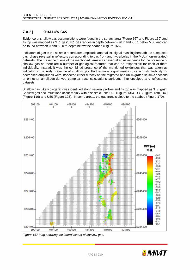
CLIENT: ENERGINET GEOPHYSICAL SURVEY REPORT LOT 1 | 103282-ENN-MMT-SUR-REP-SURVLOT1
PAGE | 210
7.8.6| SHALLOW GAS
Evidence of shallow gas accumulations were found in the survey area (Figure 167 and Figure 169) and its top was mapped as “HZ_gas”. HZ_gas ranges in depth between -26.7 and -85.1 below MSL and can be found between 0 and 58.0 m depth below the seabed (Figure 168).
Indicators of gas in the seismic record are: amplitude anomalies, signal masking beneath the suspected gas, phase reversal in reflectors corresponding to gas front and hyperbolas in the MUL (non-migrated) datasets. The presence of one of the mentioned items was never taken as evidence for the presence of shallow gas as there are a number of geological features that can be responsible for each of them individually. Instead, it was the combined presence of the mentioned evidences that was taken as indicator of the likely presence of shallow gas. Furthermore, signal masking, or acoustic turbidity, or decreased amplitudes were inspected either directly on the migrated and un-migrated seismic sections or on other amplitude-derived complex trace calculations attributes, like envelope and reflectance datasets
Shallow gas (likely biogenic) was identified along several profiles and its top was mapped as “HZ_gas”. Shallow gas accumulations occur mainly within seismic units U20 (Figure 136), U30 (Figure 128), U40 (Figure 116) and U50 (Figure 103). In some areas, the gas front is close to the seabed (Figure 170).
Figure 167 Map showing the lateral extent of shallow gas.
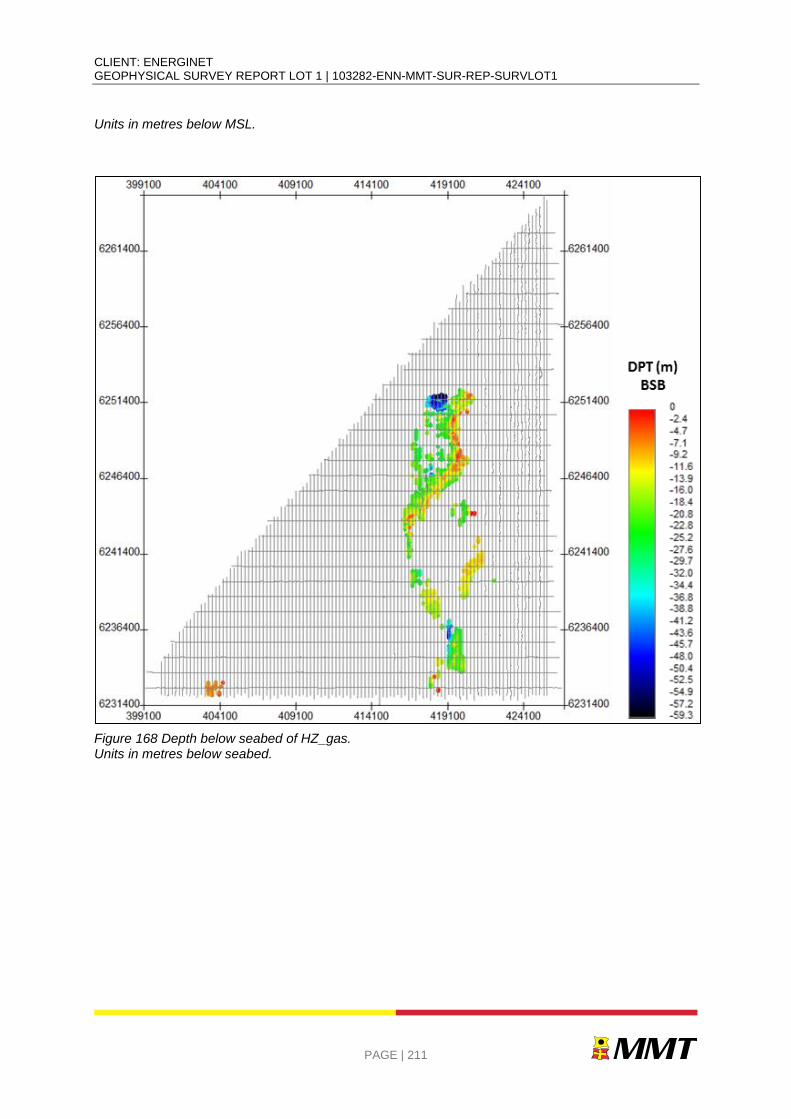
CLIENT: ENERGINET GEOPHYSICAL SURVEY REPORT LOT 1 | 103282-ENN-MMT-SUR-REP-SURVLOT1
PAGE | 211
Units in metres below MSL.
Figure 168 Depth below seabed of HZ_gas. Units in metres below seabed.
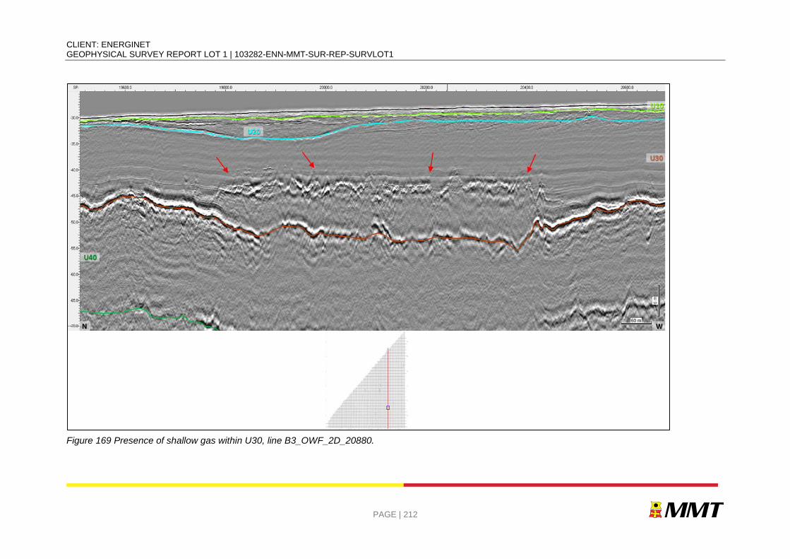
CLIENT: ENERGINET GEOPHYSICAL SURVEY REPORT LOT 1 | 103282-ENN-MMT-SUR-REP-SURVLOT1
PAGE | 212
Figure 169 Presence of shallow gas within U30, line B3_OWF_2D_20880.
CLIENT: ENERGINET GEOPHYSICAL SURVEY REPORT LOT 1 | 103282-ENN-MMT-SUR-REP-SURVLOT1
PAGE | 213
Figure 170 Profile B3_OWF_2D_2040 (a) and B3_OWF_2D_20880 (b) displaying the gas front is close to the seabed (red arrow).
CLIENT: ENERGINET GEOPHYSICAL SURVEY REPORT LOT 1 | 103282-ENN-MMT-SUR-REP-SURVLOT1
PAGE | 214
7.9| ARCHAEOLOGY CONSIDERATIONS
During the survey there was no obvious archaeological findings observed. Two historic ship wrecks (S_DH_B01_0199 and S_DH_B03_0559) have been described in Section 7.4.1|. According to the background data these sank in 1997 and1994 respectively. However, it is suggested that a full archaeology investigation be conducted on the data collected here by professionally qualified archaeologists in order to assess the possibility of paleo landscapes that could have been occupied by early man. This type of analysis is out with the scope for this report.
7.10| GEOTECHNCIAL SUMMARY
The Thor OWF area encompasses a variety of seabed conditions. Engineering within investigated depth profile below the seabed should consider the following general observations, which are neither exhaustive or prescriptive, and are related exclusively to the observed material records presented in this report:
The ground conditions within the OWF area vary from those dominated by granular sediments, largely silty gravelly SAND, through to locations which have increased cohesive contents, such that medium to high strength CLAY TILL is present. Gravel content in the recovered material is typically low, with only some thin GRAVEL layers identified in the VC. It must be highlighted that the relatively low number of VC locations in the OWF area hampers any detailed assessment of the lateral variation of ground conditions. As such, any end user of the survey data should consult all available information, such as the results of the geophysical survey and data interpretation, to satisfy themselves of any geotechnical risks that may be present. The seabed Indices for the VC at 1.00 m depth across the entire OWF area highlights the presence of CLAY TILL and CLAY at 1.00 m depth in the northern part of Block 4 and CLAY in the southern part of Block 1.
The results of the grab sampling provide good coverage of the surface seabed conditions, which are entirely granular, ranging from SAND through to sporadic areas of GRAVEL. The seabed Indices for the GS at 0.00 m depth across the entire OWF area highlights the ubiquitous presence of granular material at seabed level.
Particular 'exotic' features within a survey area may shallow seabed engineering, i.e. highly organic material, high gravel and/or cobble contents. Within the OWF area, COBBLES are rather rare in the recovered material, although their presence should not be discounted. The geophysical data and interpretation should be consulted as to whether there are significant deposits of coarse GRAVEL and/or COBBLES on the seabed. The presence of organic-rich CLAY and PEAT must also be taken into consideration, due to the undesirable thermal regime which such cohesive material can generate, together with their tendency for compressibility under load and typically low material strength. PEAT has been identified at three locations, VC-004, VC-005 and VC007. In general, the PEAT is thin, <0.24 m thick and is found >2.25 m. The only exception is the thin PEAT at VC-004 at 0.41 m to 0.62 m. The possible compressibility and engineering implications of the PEAT should be considered, and also it may be prudent to consider its potential lateral extent at those locations indicated. Whilst the thermal regime of the seabed has not been a subject of investigation in this report, the potential high thermal resistivities in organic-rich material and low strength cohesive CLAY should be borne in mind, especially with regards to any electrical cable installation activities.
For a full description of the geotechnical results please refer to the geotechnical report (103282-ENN-MMT-SUR-GEOTEC-LOT1_RevA.) in Appendix C|.
CLIENT: ENERGINET GEOPHYSICAL SURVEY REPORT LOT 1 | 103282-ENN-MMT-SUR-REP-SURVLOT1
PAGE | 215
8| CONCLUSIONS
The results of the bathymetric survey found that the water depths across the site ranged between -20.38 m and -35.43 m with depth generally increasing from the eastern extent of the site to the western extent across Lot 1.
The seabed has a range of natural topographic variability occurring throughout the site. In the eastern section of Lot 1, this is due to combination of depression areas and sediment banks, which have areas of sand wave and ripple bedforms superimposed over them. To the northwest these sediment features extend to the western site boundary. In the central and southern regions, the depths to the west of the site increase, sandwave and ripple bedforms are still present, causing undulating and disturbed seabed conditions, before the seabed flattens out and becomes featureless in the southwest of the site.
Slope angles across the site are typically very gentle (<1°) and gentle (1° to 5°). Despite the fact that sand wave areas constitute approximately 78% of the site the seafloor topography is typically gently undulating with areas of moderate to very steep gradients being largely restricted to the edges of sand bodies and the lee slopes of the most defined sand waves.
Very steep slope angles (15° to a maximum of 43°) were observed within the survey area but these were restricted to boulder features, the edges of depressions and step-like features possibly associated with sub-cropping bedrock. Higher slope angles (up to 75°) were identified, however these were associated with boulder-like features identified within Deep Helder data that could not be disproved as system noise by overlapping data.
The surficial geology in the area is dominated by sandy and gravelly sediments. They commonly range from SAND to gravelly SAND to sandy GRAVEL. In the northern parts, patches of GRAVEL are also seen.
Scattered in the northern and central parts of the investigated area are less extensive areas of DIAMICTON, interpreted to comprise a mixed sediment ranging from finer CLAY and SILT up to boulders. However, in this area, the main part of the DIAMICTON commonly consists of SAND and GRAVEL with only minor elements of SILT and CLAY. Boulders are common in the DIAMICTON areas.
In the south western part of the survey area, the seabed sediments comprise mainly SILT.
Associated with the sandy and gravelly areas are extensive areas of mobile sediments, indicating a dominating current regime from the southwest to the northeast. The mobile sediments are seen as sand waves, megaripples and ripples covering most of the survey area. Also present in conjunction with these features are areas of depressions and mass transport deposits which also are believed to be derived from the moving seabed. It is deemed that the sediment mobility in the area is overall high
The mass transport deposits are oftentimes associated with steep slopes, believed to be caused by slumping of the seabed sediments and succeeding sediment transport. The slumping causes steps in the seabed, seen as high degree slopes on the seafloor.
The areas of depressions comprise numerous depressions scattered across the seabed. Gas charged sediments are seen in the 2D UHRS data, correlating relatively well with these areas indicating a possible gas induced origin. However, these features are also commonly associated with mobile sediments and at some locations the features are elongated and begins to look like ripples. The origin of the features is therefore uncertain at this point.
In total, 9969 individual seabed contacts were detected in Lot 1.
A total of 8100 SSS contacts were detected within Lot 1. They were classified as: wrecks (2), debris (207) and boulders (7891). A total of 1255 MBES contacts were interpreted within Lot 1; and classified as MMO (5) and boulders (1250).

CLIENT: ENERGINET GEOPHYSICAL SURVEY REPORT LOT 1 | 103282-ENN-MMT-SUR-REP-SURVLOT1
PAGE | 216
A total of 622 magnetic anomalies were detected in the survey data. No anomalies were associated to known cable and pipeline infrastructure. (see Section 7.5|). The anomalies comprise one wreck and 621 discrete anomalies. Eight of the discrete anomalies correlates with SSS contacts or MBES contacts. One MAG anomaly (M_103) correlated with a known wreck and also has a correlating SSS contact (S_DH_B03_0559).
The sub seabed geology comprises the uppermost unit (U10) present at the seabed and comprises Holocene and recent sands. This unit is overlying the remaining units (U20 to U50). U20 consist of infills of depressions and/or channels, which could be related to a lagoon system and partially a subaerial fluvial infill of a low stand erosive surface. U30 and U31 have strata distinctive negative acoustic impedance contrasts at its base and could be correlated to a glaciolacustrine system. U40 is likely associated with a glaciolacustrine or a similar relatively low-energy environment. U45 could be related to a fluviodeltaic system in a moderate energy environment. U50 consists of fine layered sediments of glaciolacustrine origin and distinct laminated facies on the seismic profiles. The lowermost base unit, subdivided into SU98 and SU99, is a complex seismic unit comprising deformed sediments, which could be caused by glacial tectonics, valley infills and undeformed subparallel deltaic deposits (Miocene). Unit’s bases are erosive in nature; still minor internal erosive surfaces also occur within the units.
Alongside with the seismostratigraphic mapping, several potential geo-hazards have been interpreted within the site, such as: tectonized sediments, faulting, paleo-valley infill sediments, organic-rich deposits, coarse sediments/gravel layers and shallow gas. All of these potential hazards needs to be taken in to consideration during further planning and constructions.
Alongside with the seismostratigraphic mapping, several potential geo-hazards have been interpreted within the site, such as: tectonized sediments, faulting, paleo-valley infill sediments, organic-rich deposits, coarse sediments/gravel layers and shallow gas. All of these potential hazards needs to be taken in to consideration during further planning and constructions.
CLIENT: ENERGINET GEOPHYSICAL SURVEY REPORT LOT 1 | 103282-ENN-MMT-SUR-REP-SURVLOT1
PAGE | 217
9| RESERVATIONS AND RECOMMENDATIONS
The results in this report, both geological descriptions and contact selection, are based on interpretations of geophysical data obtained during the survey. It should be taken into account that there is a natural limitation in the accuracy of interpretation. Results from geotechnical sampling have been used for verification of the geological interpretations and is considered as ground truthing at those locations where collected. Where considered applicable, the sampling results have been extrapolated to constitute a base for verifications also in the surroundings.
Seismic interpretation presented in this report is based solely on seismic interpretation techniques. Unit definition is based on the identification and mapping of the most prominent reflectors and seismic facies shift that correspond to significant changes on depositional environments and sediment type. Seismic facies identification, internal reflector termination and geometry of the erosive surfaces are the basis for the unit’s description, inferred depositional environments and sediment type. No type of subsurface ground truthing was incorporated into the present model. All units display a certain degree of vertical and horizontal variability and heterogeneity. This is due to intrinsic nature of the geological processes that took place, the rapidly changing environment and the great extent of the site. The interpretation derived from the geophysical data should be validated by means of ground sampling (bore hole, cone penetrometer test and any soil inspection technique). Key aspects to be investigated are (1) seismic units inferred soil composition, (2) geotechnical relevance of facies shift (laterally and vertically), (3) geotechnical relevance of internal erosive surfaces, (4) importance of linear features (channels) in terms of mechanical/lithological properties and its variability, (5) mechanical relevance of the identified deformation evidences (glaciotectonics, faults, folds), (6) importance of intra-formational negative impedance contrasts, (7) presence and potential hazard of the identified gas, (8) presence of constrains in engineering and site development (boulders, coarse sediments), (9) accuracy of used depth-conversion velocity model.
Not all existing contacts are detectable in the SSS data due to resolution, material, and orientation of the object.
MMT’s recommendations for further planning within the Thor OWF are:
When the data is evaluated and more accurate positions of the planned OWF sites are decided on, a more detailed survey is recommended over the selected sites, including a full Unexploaded Ordnance (UXO) survey, visual inspection of contacts and additional geotechnical sampling.
CLIENT: ENERGINET GEOPHYSICAL SURVEY REPORT LOT 1 | 103282-ENN-MMT-SUR-REP-SURVLOT1
PAGE | 218
10| REFERENCES
Andersen, L. T. 2004. The Fanø Bugt glaciotectonic thrust fault complex, southeastern Danish North Sea. Ph.D.Thesis 2004. Danmarks og Grønlands Geologiske Undersøgelse Rapport 2004/30: 35-68.
Anthony, D. and Leth, J. O. 2001. Large-scale bedforms, sediment distribution and sand mobility in the eastern North Sea off the Danish west coast. Marine Geology 182 (2002) 247-263
Anthony, D., Møller, I. 2003. The geological architecture and development of the Holmsland Barrier and Ringkøbing Fjord area, Danish North Sea Coast. Geografisk Tidsskrift, Danish Journal of Geography 102 27
Behre, K-E, 2007. A new Holocene sea-level curve for the southern North Sea. Behre, K.-E. 2007 (January): A new Holocene sea-level curve for the southern North Sea. Boreas, Vol. 36, pp. 82-102.
Bennike, O., Jensen, J.B., Konradi, P., Lemke, W. and Heinemeier, J. 2000. Early Holocene drowned lagoonal deposits from the Kattegat, southern Scandinavia. Boreas, Vol. 29, pp. 272–286.
Bennike, O., Jensen, J.B., 1998. Late- and postglacial shore level changes in the southwestern Baltic Sea. Bulletin of the Geological Society of Denmark, Vol. 45, pp. 27-38.
Dalgas E. 1867–1868. Geografiske billeder fra Heden (H. 1 & 2).
Ehlers, J. 1990. Reconstructing the dynamics of the north-west European Pleistocene ice sheets. Quaternary Science Reviews 3: 1-40.
Fugro 2014. Fugro Seacore Limited, Energinet.dk, April 2014. Preliminary Geotechnical Investigations. Vesterhav Syd Nearshore Wind Farm. Factual Report on Ground Investigation.
Geoviden 2005. De seneste 150.000 år i Danmark. Istidslandskabets og Naturens udvikling , Nr. 2.
Houmark-Nielsen M. 2007. Extent and age of Middle and Late Pleistocene glaciations and periglacial episodes in southern Jutland, Denmark. Bull. Geol. Soc. Denmark 55: 9–35.
Høyer A-S., Jørgensen F., Piotrowski A. J., Jakobsen P. R. 2013. Deeply routed glaciotectonism in the western Denmark. Geological composition, structural charcteristics and origin Varde Hill Island. Jour. of Quat. Science 28 (7): 683-696.
Huuse, M., and Lykke-Andersen, H. 2000. Overdeepened Quaternary Valleys in the eastern Danish North Sea: morphology and origin; Quaternary Science Rewiews, vol 19 (12)
Huuse, M. and Lykke-Andersen, H. 2000b. Large-Scale glaciotectonic thrust structures in the eastern Danish North Sea Geological Society, London, Special Publications, 1010.1144/GSL.SP,2000. 176.01.22. p293-305
Jakobsen P. R. 2003. GIS based map of glaciotectonic phenomena. Denmark Geological Quarterly 47 (4): 331–338
Japsen, P. 2000. Fra Kidthav til Vesterhav. Nordsobasinets udvikling vurderet ud fra seismiske hastigheder. Geologisk Tidsskrift, haefte 2. pp. 1-36 Kobenhavn
Johannessen, P. N., Nielsen,L. H., Nielsen, L., Møller, I., Pejrup, M., Andersen, T. J., Korshøj, J., Larsen, B. and Piasecki, S. 2008. Sedimentary facies and architecture of the Holocene to Recent Rømø barrier island in the Danish Wadden Sea. Geological Survey of Denmark and Greenland Bulletin 15, 49–52.
Jørgensen, F., Sandersen, P.B.E. 2006. Buried and open tunnel valleys in Denmark erosion beneath multiple ice sheets. Quaternary Science Reviews 25, 1339–1363
CLIENT: ENERGINET GEOPHYSICAL SURVEY REPORT LOT 1 | 103282-ENN-MMT-SUR-REP-SURVLOT1
PAGE | 219
Larsen, B., and Andersen, L. T. Andersen. 2005. Late Quaternary stratigraphy and morphogenesis in the Danish eastern North Sea and its relation to onshore geology. Netherlands Journal of Geosciences 84-2, 113-128.
Leth, J.O. 1996. Late Quaternary geological development of the Jutland Bank and the initiation of the Jutland Current, NE North Sea. Nor. Geol. Unders. Bull. 430, 25-34.
Leth, J.O., Larsen, B., Anthony, D., 2004. Sediment distribution and transport in the shallow coastal waters along the west coast of Denmark Geological Survey of Denmark and Greenland Bulletin 4, 41–44.
Michelsen, O. 1993. Structural development of the Fennoscandian Border Zone, offshore Denmark. Marine and Petroleum Geology Volume 10, 24-134.
Nicolaisen, J. F. 2010. (Editor): Marin råstof- og naturtypekortlægning i Nordsøen, Naturstyrelsen.
Nielsen, L. H. Johannesen, P. 2004. Skagen Odde – et fuldskala, naturligt laboratorium. Nyt Fra GEUS, nr 1.
Nielsen, T., Mathiesen, A. and Bryde-Auken, M. 2008. Base Quaternary in the Danish part of the North Sea and Skagerrak; Geological Survey of Denmark and Greenland Bulletin 15, 37-40
Novak, B. Duarte, H. and Leth J.O. 2015. Glaciotectonic thrust complex offshore Holmsland, the Danish North Sea. Abstract in The Quaternary Geology of the North Sea, Annual discussion Meeting of the Quaternary Research association UK, Edinburgh, January, 71.
Novak B., Pedersen G. K. 2000. Sedimentology, seismic facies and stratigraphy of a Holocene spit–platform complex interpreted from high-resolution shallow seismics, Lysegrund, southern Kattegat, Denmark. Marine Geology 162, 317–335.
Novak, B. and Bjôrck S. 2002. Late Pleistocene–early Holocene fluvial facies and depositional processes in the Fehmarn Belt, between Germany and Denmark, revealed by high-resolution seismic and lithofacies analysis. Sedimentolog, 49, 451–465
Pedersen, S. A. S. 2005. Structural analysis of the Rubjerg Knude glaciotechtonic complex, Vendsyssel, Northern. Denmark. Geol. Surv. of Denmark, Bulletin 8.
Rasmussen, E. S., Dybkjær K., Piasecki S. 2010. Lithostratigraphy of the Upper Oligocene–Miocene succession of Denmark. Geological Survey of Denmark and Greenland Bulletin 22: 1–92.
Robertson, P., Campanella, R., Gillespie, D., & Greig, J. (1986). Use of Piezometer Cone. In-situ'86, Use of In-situ testing in Geotechnical Engineering, GSP 6, ASCE, Reston, 1263 - 1280.
Sandersen, P. B. E., Jørgensen F. 2003. Buried Quaternary valleys in western Denmark occurrence and inferred implications for groundwater resources and vulnerability. Journal of Applied Geophysics 53: 229– 248
Sjørring, S., Frederiksen, J. 1980. Glacialstratigrafiske observationer i de vestjyske bakkeøer. Dansk Geologisk Forenings Årsskrift 1979: 63–77.
Smed, P., 1979. Landskabskort over Danmark, Blad 1, Nordjylland. Geografforlaget, Brenderup, Denmark.
Smed, P., 1981. Landskabskort over Danmark, Blad 2, Midtjylland. Geografforlaget, Brenderup, Denmark.
Sorgenfrei, T. & Buch, A.; 1964; Deep Tests in Denmark 1935/1959. Geological Survey of Denmark, III. Series 36, Copenhagen

CLIENT: ENERGINET GEOPHYSICAL SURVEY REPORT LOT 1 | 103282-ENN-MMT-SUR-REP-SURVLOT1
PAGE | 220
Vaughan-Hirsch, D.P., Phillips, E.R. 2017. Mid-Pleistocene thin-skinned glaciotectonic thrusting of the Aberdeen Ground Formation, Central Graben region, central North Sea. Journal Of Quaternary Science, 32(2) 196–212
Vejbæk, O. V. 1997. Dybe strukturer i danske sedimentære bassiner. Geologisk Tidsskrift, hæfte 4, pp. 1-31. København, 12-16.
Vejbæk, O.V., Bidstrup, T., Erlström, M, Rasmussen, E. S. and Sivhed, M. 2007. Chalk depth structure map Central to East North Sea, Denmark. GEUS. Geological Survey of Denmark and Greenland Bulletin 13, 9-12.
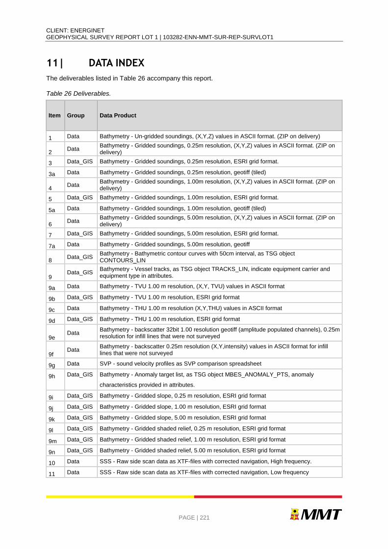
CLIENT: ENERGINET GEOPHYSICAL SURVEY REPORT LOT 1 | 103282-ENN-MMT-SUR-REP-SURVLOT1
PAGE | 221
11| DATA INDEX
The deliverables listed in Table 26 accompany this report.
Table 26 Deliverables.
Item Group Data Product
1 Data Bathymetry - Un-gridded soundings, (X,Y,Z) values in ASCII format. (ZIP on delivery)
2 Data
Bathymetry - Gridded soundings, 0.25m resolution, (X,Y,Z) values in ASCII format. (ZIP on delivery)
3 Data_GIS Bathymetry - Gridded soundings, 0.25m resolution, ESRI grid format.
3a Data Bathymetry - Gridded soundings, 0.25m resolution, geotiff (tiled)
4 Data
Bathymetry - Gridded soundings, 1.00m resolution, (X,Y,Z) values in ASCII format. (ZIP on delivery)
5 Data_GIS Bathymetry - Gridded soundings, 1.00m resolution, ESRI grid format.
5a Data Bathymetry - Gridded soundings, 1.00m resolution, geotiff (tiled)
6 Data
Bathymetry - Gridded soundings, 5.00m resolution, (X,Y,Z) values in ASCII format. (ZIP on delivery)
7 Data_GIS Bathymetry - Gridded soundings, 5.00m resolution, ESRI grid format.
7a Data Bathymetry - Gridded soundings, 5.00m resolution, geotiff
8 Data_GIS
Bathymetry - Bathymetric contour curves with 50cm interval, as TSG object CONTOURS_LIN
9 Data_GIS
Bathymetry - Vessel tracks, as TSG object TRACKS_LIN, indicate equipment carrier and equipment type in attributes.
9a Data Bathymetry - TVU 1.00 m resolution, (X,Y, TVU) values in ASCII format
9b Data_GIS Bathymetry - TVU 1.00 m resolution, ESRI grid format
9c Data Bathymetry - THU 1.00 m resolution (X,Y,THU) values in ASCII format
9d Data_GIS Bathymetry - THU 1.00 m resolution, ESRI grid format
9e Data
Bathymetry - backscatter 32bit 1.00 resolution geotiff (amplitude populated channels), 0.25m resolution for infill lines that were not surveyed
9f Data
Bathymetry - backscatter 0.25m resolution (X,Y,intensity) values in ASCII format for infill lines that were not surveyed
9g Data SVP - sound velocity profiles as SVP comparison spreadsheet
9h Data_GIS Bathymetry - Anomaly target list, as TSG object MBES_ANOMALY_PTS, anomaly
characteristics provided in attributes.
9i Data_GIS Bathymetry - Gridded slope, 0.25 m resolution, ESRI grid format
9j Data_GIS Bathymetry - Gridded slope, 1.00 m resolution, ESRI grid format
9k Data_GIS Bathymetry - Gridded slope, 5.00 m resolution, ESRI grid format
9l Data_GIS Bathymetry - Gridded shaded relief, 0.25 m resolution, ESRI grid format
9m Data_GIS Bathymetry - Gridded shaded relief, 1.00 m resolution, ESRI grid format
9n Data_GIS Bathymetry - Gridded shaded relief, 5.00 m resolution, ESRI grid format
10 Data SSS - Raw side scan data as XTF-files with corrected navigation, High frequency.
11 Data SSS - Raw side scan data as XTF-files with corrected navigation, Low frequency
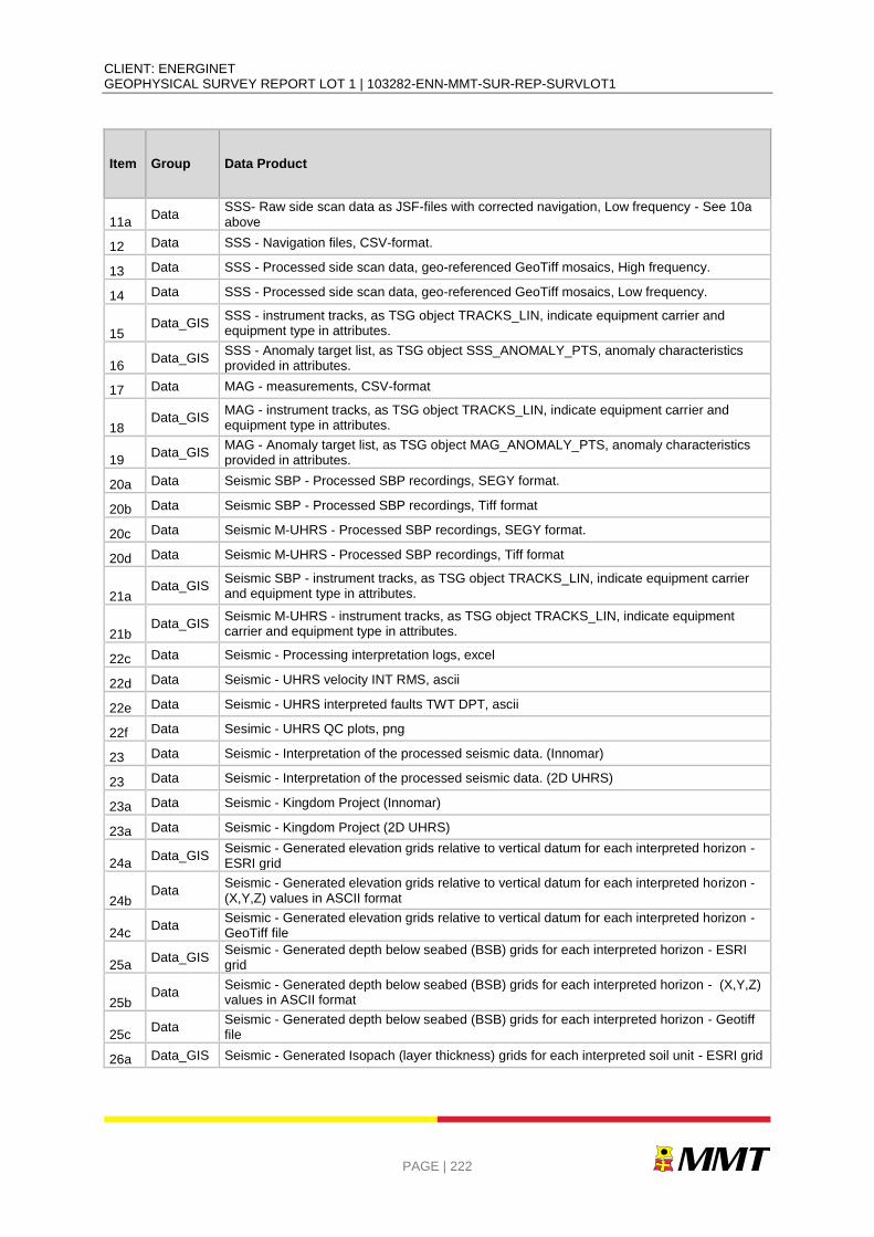
CLIENT: ENERGINET GEOPHYSICAL SURVEY REPORT LOT 1 | 103282-ENN-MMT-SUR-REP-SURVLOT1
PAGE | 222
Item Group Data Product
11a Data
SSS- Raw side scan data as JSF-files with corrected navigation, Low frequency - See 10a above
12 Data SSS - Navigation files, CSV-format.
13 Data SSS - Processed side scan data, geo-referenced GeoTiff mosaics, High frequency.
14 Data SSS - Processed side scan data, geo-referenced GeoTiff mosaics, Low frequency.
15 Data_GIS
SSS - instrument tracks, as TSG object TRACKS_LIN, indicate equipment carrier and equipment type in attributes.
16 Data_GIS
SSS - Anomaly target list, as TSG object SSS_ANOMALY_PTS, anomaly characteristics provided in attributes.
17 Data MAG - measurements, CSV-format
18 Data_GIS
MAG - instrument tracks, as TSG object TRACKS_LIN, indicate equipment carrier and equipment type in attributes.
19 Data_GIS
MAG - Anomaly target list, as TSG object MAG_ANOMALY_PTS, anomaly characteristics provided in attributes.
20a Data Seismic SBP - Processed SBP recordings, SEGY format.
20b Data Seismic SBP - Processed SBP recordings, Tiff format
20c Data Seismic M-UHRS - Processed SBP recordings, SEGY format.
20d Data Seismic M-UHRS - Processed SBP recordings, Tiff format
21a Data_GIS
Seismic SBP - instrument tracks, as TSG object TRACKS_LIN, indicate equipment carrier and equipment type in attributes.
21b Data_GIS
Seismic M-UHRS - instrument tracks, as TSG object TRACKS_LIN, indicate equipment carrier and equipment type in attributes.
22c Data Seismic - Processing interpretation logs, excel
22d Data Seismic - UHRS velocity INT RMS, ascii
22e Data Seismic - UHRS interpreted faults TWT DPT, ascii
22f Data Sesimic - UHRS QC plots, png
23 Data Seismic - Interpretation of the processed seismic data. (Innomar)
23 Data Seismic - Interpretation of the processed seismic data. (2D UHRS)
23a Data Seismic - Kingdom Project (Innomar)
23a Data Seismic - Kingdom Project (2D UHRS)
24a Data_GIS
Seismic - Generated elevation grids relative to vertical datum for each interpreted horizon - ESRI grid
24b Data
Seismic - Generated elevation grids relative to vertical datum for each interpreted horizon - (X,Y,Z) values in ASCII format
24c Data
Seismic - Generated elevation grids relative to vertical datum for each interpreted horizon - GeoTiff file
25a Data_GIS
Seismic - Generated depth below seabed (BSB) grids for each interpreted horizon - ESRI grid
25b Data
Seismic - Generated depth below seabed (BSB) grids for each interpreted horizon - (X,Y,Z) values in ASCII format
25c Data
Seismic - Generated depth below seabed (BSB) grids for each interpreted horizon - Geotiff file
26a Data_GIS Seismic - Generated Isopach (layer thickness) grids for each interpreted soil unit - ESRI grid
CLIENT: ENERGINET GEOPHYSICAL SURVEY REPORT LOT 1 | 103282-ENN-MMT-SUR-REP-SURVLOT1
PAGE | 223
Item Group Data Product
26b Data
Seismic - Generated Isopach (layer thickness) grids for each interpreted soil unit - (X,Y,Z) values in ASCII format
26c Data Seismic - Generated Isopach (layer thickness) grids for each interpreted soil unit - Geotiff file
27 Data_GIS
Grab - Grab sample positions, as TSG object GEOTECHNIC_PTS, indicate sampling characteristics in attributes.
28 Data Grab - Grab sample classification, MS-Excel spread sheet
28a Data Grab - Grab sample classification, AGS format
29 Data Grab - Grab sample laboratory analysis, overview table and result tables, PDF format.
30 Data Geotechnical sampling overview, MS-Excel spread sheet
31 Data Geotechnical results, MS-Excel spread sheet
32 Data Geotechnical results, AGS format
33 Data_GIS
Seabed Surface Geology, as TSG object SEABED_GEOLOGY_POL, indicate surface geological unit in attributes.
34 Data_GIS
Seabed Surface Features, as TSG object SEABED_SURFACE_PTS, indicate surface forms in attributes.
35 Data_GIS
Seabed Surface Features, as TSG object SEABED_SURFACE_LIN, indicate surface forms in attributes.
36 Data_GIS
Seabed Surface Features, as TSG object SEABED_SURFACE_POL, indicate surface forms in attributes.
37 Data_GIS Man-Made-Objects, as TSG object MMO_PTS, indicate MMO type in attributes
38 Data_GIS Man-Made-Objects, as TSG object MMO_LIN, indicate MMO type in attributes.
39 Data_GIS Benthic - Program point features class in ESRI File Geodatabase
40 Data_GIS Benthic - Program line features class in ESRI File Geodatabase
42 Report Operational Report
43 Report Geophysical Report & charts, drawings and enclosures
44 Report Benthic Scope Report
45 Report Project Execution Plan
46 Report Field Report (Overview sheets)

CLIENT: ENERGINET GEOPHYSICAL SURVEY REPORT LOT 1 | 103282-ENN-MMT-SUR-REP-SURVLOT1
PAGE | 224
APPENDIX A| LIST OF PRODUCED CHARTS
APPENDIX B| CONTACT AND ANOMALY LIST
APPENDIX C| GEOTECHNICAL LAB REPORT
APPENDIX D| 2D UHRS PROCESSING REPORT
APPENDIX E| BOULDER FIELDS


