SPE 155499

PVT in Liquid-Rich Shale Reservoirs Curtis Hays Whitson, NTNU & PERA and Snjezana Sunjerga, PERA

Copyright 2012, Society of Petroleum Engineers This paper was prepared for presentation at the SPE Annual Technical Conference and Exhibition held in San Antonio, Texas, USA, 8-10 October 2012. This paper was selected for presentation by an SPE program committee following review of information contained in an abstract submitted by the author(s). Contents of the paper have not been reviewed by the Society of Petroleum Engineers and are subject to correction by the author(s). The material does not necessarily reflect any position of the Society of Petroleum Engineers, its officers, or members. Electronic reproduction, distribution, or storage of any part of this paper without the written consent of the Society of Petroleum Engineers is prohibited. Permission to reproduce in print is restricted to an abstract of not more than 300 words; illustrations may not be copied. The abstract must contain conspicuous acknowledgment of SPE copyright.

Abstract This paper addresses sampling and PVT modeling of liquid-rich fluids produced from ultra-tight formations – “liquid-rich shale” (LRS) reservoirs.1 Proper PVT treatment in these unconventional reservoirs is important to provide improved short- and long-term oil and gas production forecasts, and define the initial oil and gas in place.

We give recommended practices for sampling, laboratory PVT tests, developing PVT (EOS and black-oil) models, and estimating the in-situ reservoir fluid system (composition, saturation, and initial gas-oil ratio). Fluid systems studied include a wide range from lean gas condensates to volatile oils, typical of what is found in the Eagle Ford, Avalon, and other liquid-rich shale plays in North America – with producing oil-gas ratios ranging from 10-1,000 STB/MMscf.

LRS producing wellstreams, usually expressed in this paper as a producing oil-gas ratio (OGR) or “liquid yield” 2, are always much leaner than what would be produced from a conventional, higher-permeability reservoir containing the same initial reservoir fluid system. Conventional reservoirs typically produce an initial mixture (for months or years) that is quite similar to the in-situ initial reservoir fluid. The anomalously-low producing OGR of LRS wells is due to very low permeabilities that lead to large drawdowns and fluid flow with localized and large gas-to-oil mobility ratio gradients near the fractures. We show that the loss in oil is a staggering factor of 2 to 50! The liquid yield will be approximately constant from the early days of initial testing throughout the well’s entire life.

The degree of oil recovery in LRS wells is associated mainly with two issues. First and foremost, whether the reservoir is initially saturated with oil (Soi=1-Swc) or gas (Soi=0). For example, with the in-situ solution OGR of ~350 STB/MMscf (initial GOR of ~3,000 scf/STB), the producing OGR might be 100 STB/MMscf for an oil reservoir (Soi=1-Swc), while it might be less than 10 STB/MMscf for a gas reservoir (Soi=0). Second, for oil LRS reservoirs, oil recovery loss is greatest for near-saturated initial conditions, with oil recoveries increasing as the oil reservoir becomes more undersaturated; degree of undersaturation does not have an impact on the large oil recovery losses seen in all LRS gas reservoirs.

Another important result from our study is showing how liquid yield (OGR) evolves with time for LRS wells. It is shown for planar “slab” fracture geometries that the expected infinite-acting behavior is a constant OGR that may last many years or decades. A less-constant intermediate-to-long-term OGR development is found in naturally- or induced-fracture “networks” consisting of a collection of matrix blocks surrounded by fractures. OGR variation depends on network fracture “block” size.

The paper shows that it is necessary to combine single-well, finely-gridded numerical modeling of LRS wells to properly develop valid PVT models and in-situ fluid description. Conventional “PVT” sampling and initialization procedures are alone inadequate for liquid-rich shale systems, but additionally require proper treatment of near-well reservoir flow and phase behavior to properly link the significant contrast in producing wellstreams and in-situ fluids.

Finally, we propose a special PVT laboratory test for LRS systems. Problem Statement What you produce at the surface is not what you have in the reservoir. This is the general problem for liquid-rich shales producing with large drawdowns. The typical LRS oil rate is much less than a conventional reservoir would produce at the same drawdown.

1 We do not differentiate between shale and other ultra-tight rock types, as we find no evidence that key PVT and fluid issues differ substantially because of the rock itself. Our terminology “liquid-rich shale” (LRS) applies to any reservoir system with permeability in the range 10-1,000 nD (1E-5 to 0.001 md), and where more than ~25% of revenues derive from the sale of oil or condensate. 2 Liquid yield as a term for producing OGR is a bit misleading for ultra-tight oil reservoirs because it conventionally implies STO (liquid) condenses exclusively from flowing reservoir gas. Liquid production in LRS oil reservoirs will include significant amounts of free-flowing reservoir oil.

2 SPE 155499

An LRS oil reservoir initially saturated with oil (Soi=1-Swc) will produce substantially less oil than a conventional reservoir would produce with the same drawdown. The fraction of oil produced, compared with conventional oil reservoirs, is typically a factor of 0.5 to 0.05, mainly depending on initial solution GOR and degree of undersaturation.

An LRS gas condensate reservoir initially saturated with gas (Soi=0), no matter how rich, will mainly produce only solution condensate being carried by the flowing reservoir gas (at bottomhole flowing pressure). Practically all oil forming by condensation in the reservoir will remain unproduced. Resulting condensate yields are typically in the range 1-10 STB/MMscf throughout the well’s life, the producing OGR value being mostly dependent on reservoir temperature and flowing bottomhole pressure.

An important consequence of these observations is that an LRS field with continuously-varying areal composition (in-situ GOR) variation will show an abrupt change in producing oil-gas ratios – from very low (in the gas condensate province) to rapidly increasing as one crosses into the oil province. This contrast will be greatest for highly-undersaturated fields such as Eagle Ford.

Example. Consider three wells, all having the same initial pressure, temperature, and in-situ fluid with a solution OGR of 350 STB/MMscf (initial solution GOR of 2857 scf/STB). All three wells produce a first-week gas rate of 10 MMscf/D with the same drawdown (e.g. pwf=1000 psia). Well A produces from a thin 10-md reservoir with a first-week oil rate of 3500 STB/D. Wells B and C are one-mile long horizontal wells with 100 nd permeability and 25 fractures. Well B produces from an oil-saturated reservoir at a first-week oil rate of 1000 STB/D. Well C produces from a gas-saturated reservoir at a first-week oil rate of only 200 STB/D. At $3/Mscf and $100/bbl prices, the three wells have first-week daily revenues of (A) $380,000/day, (B) $130,000/day, and (C) $50,000/day. For a dry-gas shale well, the daily revenue would be $30,000/day. Dimensionless Producing OGR

LRS wells have long periods (months, years, and sometimes more than a decade) where the production performance is similar to a well draining an “infinite” reservoir without no-flow outer boundaries (between fractures and between wells). During infinite-acting production with a constant flowing bottomhole pressure, the producing oil-gas ratio is almost constant. A significant percentage of ultimate recovery is often obtained during infinite-acting behavior of LRS wells.

We therefore introduce the dimensionless producing OGR (rpD) – a kind of oil recovery efficiency – defined as the ratio of producing OGR (rp) to initial reservoir OGR (ri): rpD=rp/ri. In terms of gas-oil ratios, rpD=Ri/Rp, or rpD= rpRi where Ri=initial reservoir solution GOR. Conventional reservoirs typically have rpD values ~1 during the infinite-acting period. The magnitude of rpD therefore represents the fraction of oil recovery obtained in an LRS reservoir compared with the oil recovery expected from a conventional reservoir after having produced the same amount of gas.

If the gas recovery factor is known at any time during the infinite-acting period (when rp~constant), then oil recovery factor (at the same time) will be RFo=rpDRFg. If the gas recovery factor (RFg) is known at any time, then oil recovery factor at the same time is given by RFo=ȓpDRFg, with averaged oil recovery efficiency given by ȓpD=(∫qg(t)rpD(t)dt)/(∫qg(t)dt).

We show in this paper that the infinite-acting behavior of LRS wells is usually characterized by oil recovery efficiencies ranging from 0.05-0.5 for volatile oils (Ri>1000 scf/STB), and 0.5-0.9 for lower-GOR/undersaturated oils. The oil recovery efficiency is also a strong function of the degree of undersaturation for oil systems, with increasing efficiency for increasing degree of undersaturation.

For a gas condensate reservoir, even near-critical, the oil recovery efficient is very low and given approximately by rpD≈ rs(pwf)/ri, where rs(pwf) is the solution OGR at the stabilized bottomhole flowing pressure pwf. The reservoir oil phase that develops through condensation will not be produced, with resulting values of rpD≈0.01-0.1.

Traditional Sampling and PVT Data Practically all wells, including LRS wells, collect basic “production” PVT data – (1) primary separator gas composition (yspi), (2) producing test gas-oil ratio (Rptest) or oil-gas ratio (rptest), (3) stock-tank oil gravity γAPI, and (4) reservoir temperature (TR). Historically, for oil reservoirs, these data were sufficient to build a PVT model using correlations, and the test producing GOR provided a good estimate of the in-situ solution GOR. Tables 1 and 2 shows these data for a liquid-rich shale well.

For traditional gas condensate reservoirs, production PVT data have not been considered sufficient to build a valid PVT model, mainly because reliable correlations do not exist for estimating dewpoint or the variation in solution oil-gas ratio rs(p). The function rs(p) is particularly important for conventional gas condensate reservoirs because the solution- and producing oil-gas ratios are similar, rs(pR)≈rp(pR), with rp(pR) seldom being less than 5-10% than rs(pR).

The traditional PVT approach for gas condensates and highly-volatile oils has been to collect reservoir samples by recombining separator gas and separator oil samples, or directly from openhole formation tester samples. These samples provide, in most cases, excellent estimates of the in-situ reservoir fluid system for oil and gas condensate reservoirs. Despite some deviation of separator-recombined and openhole formation tester samples from in-situ fluids, the uncertainties in initial solution OGR (rsi) is seldom more than ~10%, a minor uncertainty compared with LRS systems.

Laboratory tests conducted on reservoir samples include (1) constant composition expansion (CCE), (2) differential liberation (DL), (3) constant volume depletion (CVD), and sometimes (4) multi-stage separation (SEP). These tests provide basic phase and volumetric properties that can be used to directly calculate black-oil PVT properties for lower-GOR (<1500 scf/STB) oils. The lab PVT data can also be used to tune an equation of state (EOS) model which is then used to generate

SPE 155499 3

black-oil PVT properties. The oil-phase black-oil PVT are oil formation volume factor (Bo) and solution gas-oil ratio (Rs); the gas phase black-oil PVT are (“dry”) gas formation volume factor (Bgd) and solution oil-gas ratio (rs).

It is particularly difficult to calculate consistent, accurate gas PVT properties Bgd(p) and rs(p) directly from conventional CCE/DL/CVD/SEP tests, and thus the need for an EOS. The EOS-to-black-oil procedure (Whitson and Torp 1983) includes defining: (1) the EOS parameters; (2) a reservoir fluid composition; (3) the method of depletion (CCE/DL/CVD); and (4) the surface separation process (e.g. number of stages and conditions of each stage). Many reservoirs require extrapolation of saturated properties beyond the saturation pressure of collected samples. Liquid-Rich Sampling and PVT Data

Collecting samples from any well generally has two main purposes – (1) supplying samples to measure PVT data which can be used to tune an EOS model and develop black-oil PVT tables, and (2) collecting a sample that reflects the in-situ reservoir fluid. Both sampling issues are addressed for LRS wells.

Sampling. The producing OGR of LRS wells drops rapidly as the well is drawn down to flowing BHPs below in-situ saturation pressure (pwf<ps). This will be illustrated by a number of simulated examples.

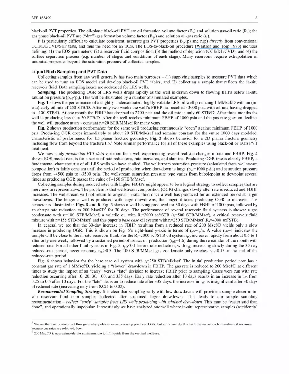
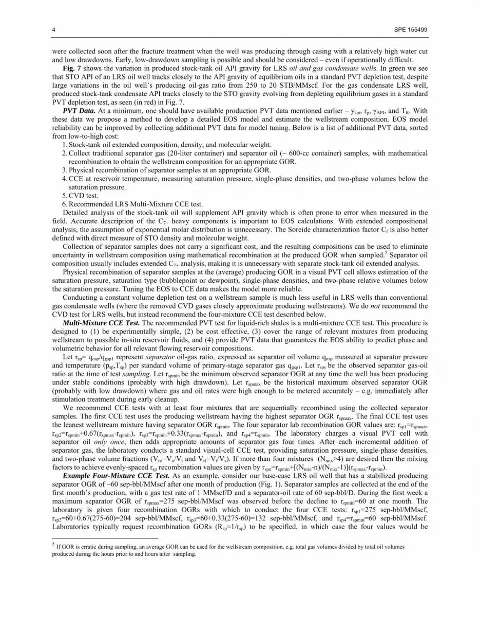
Fig. 1 shows the performance of a slightly-undersaturated, highly-volatile LRS oil well producing 1 MMscf/D with an (in-situ) early oil rate of 250 STB/D. After only two weeks the well’s FBHP has reached ~3000 psia with oil rate having dropped to ~100 STB/D. At one month the FBHP has dropped to 2700 psia and the oil rate is only 60 STB/D. After three months the well is producing less than 30 STB/D. After the well reaches minimum FBHP of 1000 psia and the gas rate goes on decline, the well will produce at an ~ constant rp=20 STB/MMscf for many years.

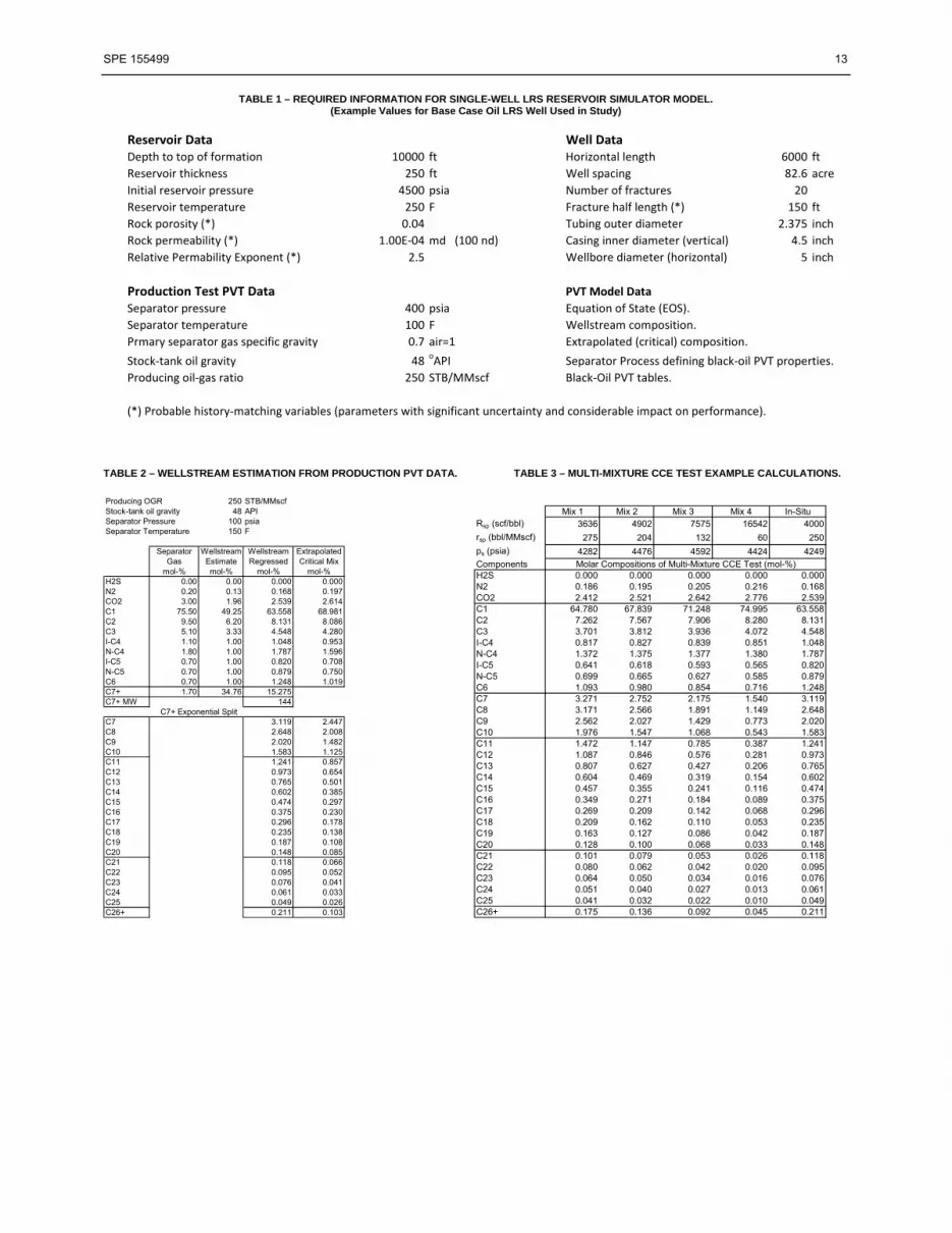
Fig. 2 shows production performance for the same well producing continuously “open” against minimum FBHP of 1000 psia. Producing OGR drops immediately to about 20 STB/MMscf and remains constant for the entire 1000 days modeled, characteristic of performance for 1D planar fracture geometry. Fig. 3 shows behavior for a 2D planar fracture geometry including flow from beyond the fracture tip.3 Note similar performance for all of these examples using black-oil or EOS PVT treatment.

We now study production PVT data variation for a well experiencing several realistic changes in rate and FBHP. Fig. 4 shows EOS model results for a series of rate reductions, rate increases, and shut-ins. Producing OGR tracks closely FBHP, a fundamental characteristic of all LRS wells we have studied. The wellstream saturation pressure (calculated from wellstream composition) is fairly constant until the period of production when drawdown is large (pwf=1000 psia) and saturation pressure drops from ~4500 psia to ~3500 psia. The wellstream saturation pressure type varies from bubblepoint to dewpoint several times as producing OGR passes the value of ~150 STB/MMscf.

Collecting samples during reduced rates with higher FBHPs might appear to be a logical strategy to collect samples that are more in-situ representative. The problem is that wellstream composition (OGR) changes slowly after rate is reduced and FBHP increases. The wellstream will not return to original in-situ fluid once a well has produced for an extended period at larger drawdowns. The longer a well is produced with large drawdowns, the longer it takes producing OGR to increase. This behavior is illustrated in Figs. 5 and 6. Fig. 5 shows a well having produced for 30 days with FBHP of 1000 psia, followed by an abrupt rate reduction to 200 Mscf/D4 for 30 days. The performance of several reservoir fluid systems is shown: a gas condensate with ri=100 STB/MMscf, a volatile oil with Ri=2000 scf/STB (ri=500 STB/MMscf), a critical reservoir fluid mixture with ri=155 STB/MMscf, and this paper’s base case oil system with ri=250 STB/MMscf (Ri=4000 scf/STB).

In general we see that the 30-day increase in FBHP resulting from a reduced rate of 200 Mscf/D yields only a slow increase in producing OGR. This is shown on Fig. 5’s right-hand y-axis in terms of rpD=rp/ri. A value rpD=1 indicates the sample will be close to the in-situ reservoir fluid. For the Ri=2000 scf/STB oil system rpD increases rapidly from about 0.6 to 1 after only one week, followed by a sustained period of excess oil production (rpD~1.6) during the remainder of the month with reduced rate. For all other fluid systems in Fig. 5, rpD<0.1 before rate reduction, with rpD increasing slowly during the 30-day reduced-rate period, never reaching rpD>0.5. The 100 STB/MMscf gas condensate only reaches rpD~0.15 at the end of the reduced-rate period.

Fig. 6 shows behavior for the base-case oil system with ri=250 STB/MMscf. The initial production period now has a constant gas rate of 1 MMscf/D, yielding a “slower” drawdown in FBHP. The gas rate is reduced to 200 Mscf/D at different times to study the impact of an “early” versus “late” decision to increase FBHP prior to sampling. Cases were run with rate reduction occurring after 10, 20, 30, 100, and 335 days. Early rate reduction after 10 days results in an increase in rpD from 0.25 to 0.6 after 10 days. For the “late” decision to reduce rate after 335 days, the increase in rpD is insignificant after 30 days of reduced rate (increasing only from 0.025 to 0.03).

Recommended Sampling Strategy. It is clear that sampling early with low drawdowns will provide a sample closer to in-situ reservoir fluid than samples collected after sustained larger drawdowns. This leads to our simple sampling recommendation – collect “early” samples from LRS wells producing with minimal drawdown. This may be “easier said than done”, and operationally unpopular. Interestingly we have analyzed one well where in-situ representative samples (accidently)

3 We see that the more-correct flow geometry yields an ever-increasing produced OGR, but unfortunately this has little impact on bottom-line oil revenues because gas rates are relatively low. 4 200 Mscf/D is approximately the minimum rate to lift liquids from the vertical wellbore.

4 SPE 155499

were collected soon after the fracture treatment when the well was producing through casing with a relatively high water cut and low drawdowns. Early, low-drawdown sampling is possible and should be considered – even if operationally difficult.

Fig. 7 shows the variation in produced stock-tank oil API gravity for LRS oil and gas condensate wells. In green we see that STO API of an LRS oil well tracks closely to the API gravity of equilibrium oils in a standard PVT depletion test, despite large variations in the oil well’s producing oil-gas ratio from 250 to 20 STB/MMscf. For the gas condensate LRS well, produced stock-tank condensate API tracks closely to the STO gravity evolving from depleting equilibrium gases in a standard PVT depletion test, as seen (in red) in Fig. 7.

PVT Data. At a minimum, one should have available production PVT data mentioned earlier – yspi, rp, γAPI, and TR. With these data we propose a method to develop a detailed EOS model and estimate the wellstream composition. EOS model reliability can be improved by collecting additional PVT data for model tuning. Below is a list of additional PVT data, sorted from low-to-high cost:

1. Stock-tank oil extended composition, density, and molecular weight. 2. Collect traditional separator gas (20-liter container) and separator oil (~ 600-cc container) samples, with mathematical

recombination to obtain the wellstream composition for an appropriate GOR. 3. Physical recombination of separator samples at an appropriate GOR. 4. CCE at reservoir temperature, measuring saturation pressure, single-phase densities, and two-phase volumes below the

saturation pressure. 5. CVD test. 6. Recommended LRS Multi-Mixture CCE test. Detailed analysis of the stock-tank oil will supplement API gravity which is often prone to error when measured in the

field. Accurate description of the C7+ heavy components is important to EOS calculations. With extended compositional analysis, the assumption of exponential molar distribution is unnecessary. The Soreide characterization factor Cf is also better defined with direct measure of STO density and molecular weight.

Collection of separator samples does not carry a significant cost, and the resulting compositions can be used to eliminate uncertainty in wellstream composition using mathematical recombination at the produced GOR when sampled.5 Separator oil composition usually includes extended C7+ analysis, making it is unnecessary with separate stock-tank oil extended analysis.

Physical recombination of separator samples at the (average) producing GOR in a visual PVT cell allows estimation of the saturation pressure, saturation type (bubblepoint or dewpoint), single-phase densities, and two-phase relative volumes below the saturation pressure. Tuning the EOS to CCE data makes the model more reliable.

Conducting a constant volume depletion test on a wellstream sample is much less useful in LRS wells than conventional gas condensate wells (where the removed CVD gases closely approximate producing wellstreams). We do not recommend the CVD test for LRS wells, but instead recommend the four-mixture CCE test described below.

Multi-Mixture CCE Test. The recommended PVT test for liquid-rich shales is a multi-mixture CCE test. This procedure is designed to (1) be experimentally simple, (2) be cost effective, (3) cover the range of relevant mixtures from producing wellstream to possible in-situ reservoir fluids, and (4) provide PVT data that guarantees the EOS ability to predict phase and volumetric behavior for all relevant flowing reservoir compositions.

Let rsp= qosp/qgsp1 represent separator oil-gas ratio, expressed as separator oil volume qosp measured at separator pressure and temperature (psp,Tsp) per standard volume of primary-stage separator gas qgsp1. Let rsps

be the observed separator gas-oil ratio at the time of test sampling. Let rspmin

be the minimum observed separator OGR at any time the well has been producing under stable conditions (probably with high drawdown). Let rspmax

be the historical maximum observed separator OGR (probably with low drawdown) where gas and oil rates were high enough to be metered accurately – e.g. immediately after stimulation treatment during early cleanup.

We recommend CCE tests with at least four mixtures that are sequentially recombined using the collected separator samples. The first CCE test uses the producing wellstream having the highest separator OGR rspmax. The final CCE test uses the leanest wellstream mixture having separator OGR rspmin. The four separator lab recombination GOR values are: rsp1=rspmax, rsp2=rspmin+0.67(rspmax-rspmin), rsp3=rspmin+0.33(rspmax-rspmin), and rsp4=rspmin. The laboratory charges a visual PVT cell with separator oil only once, then adds appropriate amounts of separator gas four times. After each incremental addition of separator gas, the laboratory conducts a standard visual-cell CCE test, providing saturation pressure, single-phase densities, and two-phase volume fractions (Vro=Vo/Vt and Vrt=Vt/Vs). If more than four mixtures (Nmix>4) are desired then the mixing factors to achieve evenly-spaced rsp recombination values are given by rspn=rspmin+[(Nmix-n)/(Nmix-1)](rspmax-rspmin).

Example Four-Mixture CCE Test. As an example, consider our base-case LRS oil well that has a stabilized producing separator OGR of ~60 sep-bbl/MMscf after one month of production (Fig. 1). Separator samples are collected at the end of the first month’s production, with a gas test rate of 1 MMscf/D and a separator-oil rate of 60 sep-bbl/D. During the first week a maximum separator OGR of rspmax=275 sep-bbl/MMscf was observed before the decline to rspmin=60 at one month. The laboratory is given four recombination OGRs with which to conduct the four CCE tests: rsp1=275 sep-bbl/MMscf, rsp2=60+0.67(275-60)=204 sep-bbl/MMscf, rsp3=60+0.33(275-60)=132 sep-bbl/MMscf, and rsp4=rspmin=60 sep-bbl/MMscf. Laboratories typically request recombination GORs (Rsp=1/rsp) to be specified, in which case the four values would be

5 If GOR is erratic during sampling, an average GOR can be used for the wellstream composition, e.g. total gas volumes divided by total oil volumes produced during the hours prior to and hours after sampling.

SPE 155499 5

Rsp1=1E6/275=3636 scf/sep-bbl, Rsp2=1E6/204=4902 scf/sep-bbl, Rsp3=1E6/132=7575 scf/sep-bbl, Rsp4=1E6/60=16,670 scf/sep-bbl.

Table 3 and Fig. 8 show the results from the simulated Four-mixture CCE test. The oil relative volume curves shown in Fig. 8 illustrate that the range of mixtures covers lean gas condensate to near-critical gas and oil behavior, with the first mixture being quite similar to the actual in-situ reservoir fluid system; Mixture 1 composition does have some differences from the in-situ oil, particularly for methane and light-intermediates C2-C4 (Table 3).

Multi-Mixture CCE Test – Additional Considerations. If the minimum separator OGR is less than the producing OGR at the time of sample collection (rsps), and you want one of the mixtures used in the multi-CCE test to represent the produced wellstream at time of sampling, either add this mixture to the set of four already designed mixtures, or simply replace one of the design mixtures that has a OGR similar to that during sampling (rspn~rsps).

If separator samples are collected before the well has seen larger drawdowns and the minimum stabilized producing OGR is still quite high, then we recommend using a default minimum rspmin~30 sep-bbl/MMscf. Furthermore, if a well has only seen large drawdowns and lower producing OGRs, we recommend using a default maximum rspmax~350 sep-bbl/MMscf.

The final mixture can be equilibrated at a pressure of ~1500 psia, with compositions measured on the equilibrium gas and equilibrium oil. Oil viscosity can also be measured on the equilibrium oil, if sufficient sample is available.6 These additional tests will cost extra, but the resulting data provide relevant information for the flowing reservoir mixture, and they need only be measured on a few samples in a given field.

An EOS model that matches the PVT data outlined above, and the multi-mixture CCE test in particular, should be reliable for describing a wide range of fluids from the same reservoir. EOS Modeling with Production Test PVT Data A method is proposed to develop a reliable EOS model from limited production test PVT data. The EOS can be used to make initial modeling studies of liquid-rich production performance, initial fluid system estimation, and generating consistent black-oil PVT tables.

A reliable EOS requires knowledge of composition and some key PVT properties with which the EOS predictions can be verified. Compositional data for LRS wells is known, indirectly, from the three data yspi, rp, and γAPI. Separator gas composition defines the relative amounts of lighter components N2, CO2, C1, C2, C3, i-C4, n-C4, i-C5, n-C5, and C6 in the wellstream. The producing OGR defines approximately the wellstream C7+ amount. The STO API gravity defines the C7+ “characterization”.

Our method relies on finding a wellstream composition zwi that, when input to the developed EOS, reproduces exactly the production PVT data rp, γAPI, and yspi. The EOS components include light fractions through C5, and heavier fractions C6, C7, …, CN+ (typically C26+). An exponential molar distribution is assumed for C7+, defined by its molecular weight M7+. The Soreide C7+ characterization parameter, Cf, is used to define the relation between C6+ SCN specific gravities and molecular weights (Whitson and Brule 2000).

We use an efficient non-linear regression algorithm in the EOS-based software (Zick Technologies 2012) to solve simultaneously for N+1 unknowns (zwi,i=1…N-1, fgw, M7+) using the N+1 data (yspi,i=1…N-1, rp, γAPI), where zwi=fgwyspi+(1-fgw)xspi

and fgw is the mole fraction of wellstream becoming separator gas. An initial guess of the wellstream composition (żwi) can be calculated with an estimate ḟgw calculated from the producing OGR, ḟgw≈(1+Cogrp)

-1, with rp in STB/scf, Cog=133,000(γo/Mo) and γo=141.5/(131.5+γAPI). The Cragoe (1929) correlation can be used to estimate STO molecular weight, Mo=6084/(γAPI-5.9). Our initial wellstream estimates are żwi =ḟgwyspi

for lighter components through C4 and żw7+=1-ḟg; for i-C5, n-C5 and C6, żwi are assumed equal and constrained by ∑żwi=1.

We normally use the Soave-Redlich-Kwong (Soave 1972) EOS with zero binary interaction parameters (BIPs) between all hydrocarbons, but the Peng-Robinson (Peng and Robinson 1976) with slightly positive methane-C7+ BIPs can also be used (see Whitson and Brule for recommended EOS default BIPs). Table 2 shows the results of this procedure for production test data given in Table 1. Because measured saturation pressure and type (dewpoint or bubblepoint) are not available from production test PVT data, it is not recommended to adjust C1-C7+ BIPs.7

Black-Oil Table Creation. The black-oil table is created from a composition (zBO) and an appropriate EOS. We use a CCE depletion process, and appropriate separator conditions for the given field. It is a good idea to use the same separator conditions for all samples in a field, so that all wells have a consistent definition of surface gas and surface oil. This allows rates to be handled consistently from several black-oil models in the same field/area.

Approximate Surface Process. A good alternative to using an EOS-based multi-stage separator process is to assume C(n-1)- defines surface gas and Cn+ defines surface oil – e.g. (C4- and C5+) or (C5- and C6+): using z(n-1)-≈(1+Cogrp)

-1. This approximation should provide reasonable oil-gas ratios compared with a standard 2- or 3-stage separator process, with Cog assumed constant (typically~700-900 scf/STB) and readily calculated from one sample where composition and OGR are

6 If sufficient equilibrium oil sample is not available for viscosity measurement, we recommend measuring oil viscosity on the separator oil directly, but at reservoir temperature and pressures in the range of 500 to 2000 psia, typical of near-fracture flowing pressures. 7 Because a measured saturation pressure and type (dewpoint or bubblepoint) are not available from production test PVT data, it is not recommended to adjust C1-C7+ BIPs. We may allow some modification of the default C1-C7+ BIPs to satisfy a constraint that saturation pressure not exceed initial reservoir pressure, this being based on our observation from compositional well modeling studies that the condition (psw≤pRi) is usually met.

6 SPE 155499

known for a particular separator. This approximate surface process is simple and consistent, and makes it possible to convert any new wellstream to an approximate oil-gas ratio equivalent without using an EOS-based PVT program.

Extrapolating Black-Oil Tables. We strongly recommend extrapolating the saturated gas and oil black-oil PVT properties to a maximum saturation pressure (psmax) where gas and oil properties approach each other. At this critical point, Rs=1/rs and Bo= Bgd/rs. The best way to extrapolate saturated properties for LRS systems is to add increments of the incipient phase from each new elevated saturation pressure, starting with the incipient phase of zBO at its saturation pressure of (ps(zBO)).

An extrapolated critical mixture is needed to ensure that single-phase initialization can be achieved for any initial solution OGR (ri). Without extrapolation to a critical point, a range of initial fluids compositions (ri) would exist where the fluid system must be initialized as a saturated two-phase gas-oil system; namely, in the range rs(ps(zBO))<ri<1/Rs(ps(zBO)) where rs(ps(zBO)) and 1/Rs(ps(zBO)) are solution oil-gas ratios of zBO and its incipient phase.

The ability to initialize a black-oil model with any solution OGR for undersaturated reservoirs (such as Eagle Ford) is important when history matching production performance (rp(t)) using the initial solution OGR ri as a history-matching variable.

Example EOS Model from Production PVT Data. An example is given to illustrate how simple, basic production PVT data can be used to generate an EOS model. Tables 1 and 2 give data yspi, rp, and γAPI with their origin in a publication8 by an Eagle Ford operator (Orangi et al. 2011) describing “approximate” Eagle Ford PVT data. Our proposed method described above was used to generate an EOS model (Table 4) with components through C26+.

This EOS should provide a reasonable model for predicting Eagle Ford PVT properties, in lieu of developing a more-rigorous EOS model using actual production (and special) PVT data from many wells in the Eagle Ford field. Table 5 gives a range of compositions from leaner gas condensate to lower-GOR oils, based on our EOS model and assumptions that (a) C6- component distribution is the same as generated for our base-case wellstream mixture in Tables 1 and 2, and (b) a simple empirical relation exists between stock-tank oil API and in-situ OGR (ri=rs or 1/Rs): γAPI=-7.5log (ri)+62.5.

Fig. 9 shows a p-T phase diagram for our estimated wellstream mixture, with predicted bubblepoint of 4754 psia at 250oF, and a critical point of 4182 psia at 380 oF. Incipient gas from this oil’s bubblepoint was added in sufficient amount to increase the saturation pressure to a critical condition at 250oF, with the resulting composition given in Table 2. Without this critical-point extrapolation, initial OGRs that could be used to initialize a single-phase model would be limited to oils with rsi≥250 STB/MMscf (of the wellstream oil) and gas condensates with rsi≤90 STB/MMscf (of the incipient gas). Any in-situ OGR in the range 90<ri<250 STB/MMscf would have to be initialized as a two-phase saturated gas-oil reservoir. Such a saturated gas-oil initialization would be physically inconsistent for Eagle Ford which is highly undersaturated.

Figs. 10-13 show black-oil PVT properties that have been generated from our EOS model. A CCE test was simulated with the extrapolated critical mixture, where equilibrium gases and equilibrium oils were independently passed through a two-stage separator process: Tsp1=150oF, psp1=100 psia and Tsp2=60oF, psp2=14.7 psia (according to the Whitson-Torp method).

The solution OGR chart (Fig. 12) defines how solution GOR of the oil phase varies with bubblepoint pressure, 1/Rs(pb), and how solution OGR of the gas phase varies with dewpoint pressure, rs(pd). This curve is, in reality, a pressure-composition phase diagram where composition is represented by solution OGR (expressed as z5- or z6+) and pressure is saturation pressure (dewpoint or bubblepoint); see lower part of Fig. 12.

EOS Modeling with Additional PVT Data With additional PVT data available, such as the Four-Mixture CCE test, the EOS model can be fine-tuned to provide more confidence in predicting phase and volumetric properties for a wider range of pressure and composition. A single EOS may be capable of describing many, if not all, reservoir fluids in a given province – such as Eagle Ford or Avalon – where composition varies spatially from dry gas to gas condensate to oil, and the in-situ fluid system may be single phase or saturated two-phase gas+oil.

To establish whether a common field-wide EOS model can be used, several samples with varying composition should be collected using the guidelines given above, with laboratory PVT data measured on each sample. The collection of PVT data can then be matched simultaneously to a common EOS model. Having a common field-wide EOS model can be helpful in defining the in-situ fluid system of a given well, generating well- or area-specific black-oil tables, and providing consistency in surface process design optimization for multi-well process facilities. Modeling Liquid-Rich Shale Wells In this study we have conducted numerical modeling of liquid-rich shale wells using a finite-difference simulator (Coats Engineering 2012). Fully implicit black-oil and compositional models produce very similar results. Numerical gridding is particularly important for LRS wells which exhibit highly-localized gas-oil flow where severe oscillation of rates and GOR is endemic if not enough grids are used. We use geometric grid spacing where rock grid sizes increase away from the fracture, as illustrated by the example in Table 6.

8 The EOS developed in our paper for Eagle Ford is based only on (a) the production PVT taken from the Orangi paper, and (b) a separator gas composition created from that paper’s EOS model. We do not use in any way either of the two EOS models given in that paper, as we do not believe it is natural or necessary to have a separate EOS model for oil and gas condensate regions of a field.

SPE 155499 7

Fractures are also gridded, with sufficiently high permeability to yield the desired pressure drop within fractures (fracture conductivity is 1000 md-ft in this study). The fracture pore volume is based on 25% porosity and a fracture width of ~0.01 ft or 3 mm. The numerical fracture width may be 0.1 or even 1 ft without having any real impact on results, as long as actual fracture conductivity and volume are honored.

We assume traditional rock relative permeabilities are applicable to shales and ultra-tight rocks. Examples in the paper use saturation exponents of 2.5. Concepts of critical gas and residual oil saturations are also assumed to be valid. We are unaware of experimental two-phase gas-oil flow tests in ultra-tight rocks that contradict the use of traditional relative permeability curves. Furthermore, the most important LRS flow region is near fractures where some micro-fracturing may exist after hydraulic fracturing, and relative permeabilities may be somewhat improved (lower saturation exponents) compared with pure-rock curves.

We ignore desorption because it is unclear whether liquid-rich systems have more or less sorption than dry gas reservoirs, and because models for desorption of components heavier than methane are limited. Some literature suggests that heavier components reduce sorption, relative to methane-rich systems. If one considers sorption in LRS wells, a consistent model is needed to describe the sorption parameters of each component, and component-component sorption interaction.

Table 1 summarizes the minimum data needed to build a single-well model. The black-oil PVT table is an important model input, together with the definition of initial fluid system (initial oil-gas ratio or initial oil-gas saturation).

Fracture Geometries. As sketched in Fig. 14, two fundamental well geometries have been considered in our study, with the horizontal well always being in the x-direction. We model only one side of the wellbore because of symmetry. Each fracture behaves independently, also due to symmetry, so only one fracture needs to be modeled and well rate equals twice the half-model rate time the total number of fractures (Nf).

Fractures emanate from single “points” along the wellbore into one of two fracture geometries: (1) planar fractures: singular fractures that penetrate the entire formation height (h) and extend a distance9 Lf away from the wellbore, symmetrically away from each side of the wellbore; and (2) network fracture: square parallelepipeds of height h and fracture-block size Lb equal in both x- and y-directions. A fracture does not run along the entire wellbore, so well connections are used only at cells where perpendicular fractures intersect the wellbore. The network fracture is defined by a half-fracture surface area Af and matrix block size Lb. If the specified half-fracture area does not exactly create a whole number of blocks, "fingers" grow outward in the y-direction from the last row of blocks; these fingers make up for the fracture area not covered by the whole blocks.

For planar fractures, we use two types of models in this work: (1) a simplified 1D model that ignores any volume beyond the tip of the fracture, resulting in one-dimensional flow in the x-direction. For early-time infinite-acting study of production performance, the 1D assumption is useful, as it allows grid refinement to a numerically-converged solution. The second planar model is 2D (x-y), taking into account the contribution from volumes beyond the fracture tip (y-direction).

Fracture Area Definitions. Half-fracture area is usually defined as Af=hLf where Lf is the total “walked” length of the half-fracture. In reality, Af is only ¼ of the full-fracture inflow area (Aff=4Af). A planar fracture has total fracture extent of 2Lf (both sides of the wellbore), and flow enters from both sides of the fracture, so Aff=4hLf. During the extended infinite-acting life of most LRS wells, fracture size (expressed as Aff, Af or Lf) and rock permeability k are the first-order parameters that determine well performance10, with fracture geometry playing a secondary role; flow is essentially one-dimensional, perpendicular to all fracture faces.

Much of the literature is ambiguous about reported well fracture areas, whether they use Afw=2NfAf or 2NfAff. We use well fracture area Afw=2NfAf. Producing OGR Behavior The producing oil-gas ratio (liquid yield) of LRS wells often remains ~constant for months or years, showing only slow variations over time. Liquid yield behavior is shown in Figs. 1-5 for our base-case LRS oil well with 20 fractures, k=100 nd, h=250 ft, and individual half-fracture area Af=37,500 ft2 (well Afw=2NfAf=1.5E6 ft2): planar fracture geometry with Lf=150 ft, and two network fracture models (a single Lb=50-ft block, and two Lb=30-ft blocks along the wellbore). The time horizon is mostly 1000 days. Unless otherwise stated, the production performance is given for a well producing with constant FBHP of 1000 psia.

Grid Sensitivity. Fig. 15 shows the impact of gridding11 perpendicular to the fracture for a 1D planar fracture. OGR oscillations are significant for less than 31 grids. With 101 grids, rp(t) doesn’t show oscillations but its value is 20 STB/MMscf, 10% higher than the converged solution of 18 STB/MMscf. Non-oscillating OGR behavior can still yield rp values 10-15% different than the converged solution.

9 By convention the term xf is used to represent fracture half-length for a planar fracture. Because our grid is oriented with x-direction along the wellbore and y-direction along which the planar fracture grows, we use Lf to represent what is normally called xf. The term Lf is also our term for any fracture geometry “walked length”. 10 Infinite-acting performance is actually controlled by the number of fractures and the fracture “productivity” term Af√k or Lf√k. 11 Note that total grids in the x-direction, Nx, are for both sides of the fracture, and because of symmetry the actual number of grids for a given case is in fact (Nx-1)/2, e.g. 15 grids are needed away from the fracture for Nx=31.

8 SPE 155499

Fig. 16 shows the difference in production performance for 1D and 2D planar fracture models. After about one month the 2D solution shows slowly-increasing OGR, compared with the constant-OGR 1D solution. The difference becomes significant by 1000 days (2D: 32 STB/MMscf vs 1D: 19 STB/MMscf). The same Nx=151 gridding was used in both 1D and 2D models, with Ny=36 for the 2D case.

Fracture Geometry. Fig. 17 shows production performance for the 1D and 2D planar fracture models, now comparing with two network fracture models: NF50, a single Lb=50-ft block, and NF30, two Lb=30-ft blocks along the wellbore. The network fracture models both show very-early-time rp(t) behavior that is somewhat higher than the two planar fracture models. This suggests insufficient gridding within the matrix blocks. When considering this slight shift in early-time rp(t) behavior we conclude for this example that the 2D planar and network fracture models have similar rp(t) behavior. The network fracture OGR increases more rapidly than the 2D planar model, as depletion effects are more significant. As matrix blocks become smaller the difference in rp(t) will become more significant. Achieving sufficient gridding to obtain a converged numerical solution becomes difficult for more and smaller matrix blocks in the network fracture model, particularly for LRS wells with complex two-phase gas-oil flow.

Oil LRS Wells. Fig. 18 shows production performance for the base-case oil LRS well with different degrees of undersaturation (using a 1D planar model). In all cases rp(t) is constant throughout the first 1000 days. As mentioned earlier, this behavior appears fundamental for 1D constant-FBHP conditions.12 Higher oil rates result for oil reservoirs that are more undersaturated because reservoir pressure is higher, and because producing OGR is higher.

Fig. 19 shows rp(t) for a 1D planar-fracture LRS well initialized with different oils (Ri) and varying degree of undersaturation. The dimensionless producing OGR rpD at 1000 days ranges from 0.02-0.6 for a wide range of initially-saturated oil systems; from 0.1-0.9 for undersaturated oils with pRi=6,000 psia; and from 0.6 to ~1 for highly-undersaturated oils with pRi=10,000 psia.

Gas Condensate LRS Wells. Fig. 20 shows production performance for two gas condensate LRS wells using a 1D planar model: a near-critical fluid with ri=155 STB/MMscf and a lean gas condensate with ri=50 STB/MMscf. The rate performance is very similar. The leaner gas condensate has slightly higher gas rates than the richer system, presumably because of relative permeability (“blockage”) effects. The producing OGRs are almost identical for the two systems, with rp≈rs(pwf)=3 STB/MMscf. Because gas rate is higher for the leaner gas condensate well, the oil rate is also higher for the leaner fluid.

Summary OGR Behavior of LRS Wells. To summarize the observations made above for oil and gas condensate LRS wells, a large number of simulations with constant FBHP of 1000 psia were made for many fluid systems at varying degrees of undersaturation. We used the 1D planar model, but similar results are found for 2D planar models (albeit somewhat higher producing OGRs at later times). Fig. 21 shows the dimensionless producing OGR (“oil recovery efficiency”) at 1000 days as a function of initial fluid OGR (ri).

For oil systems, the oil recovery efficiency rpD varies from values lower than 0.05, approaching 0.5-1 for highly undersaturated and/or low-GOR (high solution OGR) oil LRS wells. As the system approaches a critical mixture with ~150 STB/MMscf solution OGR, the oil recovery efficiency is at its lowest level, and significant undersaturation is required to achieve higher oil production performance.

For all gas condensate LRS wells simulated, independent of how undersaturated13, the oil recovery efficiency rpD was low, and fell on the trend defined by the blue line in Fig. 21 representing the ratio rpD=rs(pwf)/ri. Because rs(pwf)=3.3 STB/MMscf at pwf=1000 psia for this fluid system, the blue-curve rpD variation is exclusively caused by variation in initial OGR ri.

Effect of Constant FBHP. Fig. 22 shows model runs where the wells were produced against a constant FBHP using the 1D planar geometry. Values of constant FBHP ranged from 500 to 4000 psia. Fig. 23 plots infinite-acting producing OGR at 1000 days for a wide range of fluid systems. All gas condensate LRS wells produced with the same behavior, rp=rs(pwf). Oil LRS wells producing with FBHPs greater than 2500 psia have OGRs somewhat greater than the initial solution OGR (rpD>1). As the constraining FBHP drops below about 2500 psia we see all oil systems producing with lower OGRs than in solution (rpD<1).

Constant Gas Rate Performance. We now consider constant gas rate control for ~1 year, until minimum FBHP of 1000 psia is reached. This leads to a gradual reduction in FBHP that has a pronounced effect on producing OGR. Fig. 24 shows production performance behavior for three LRS wells: an oil, a near-critical fluid, and a gas-condensate. Fig. 25 translates the results into a plot of producing OGR versus FBHP. Gas condensate LRS wells and the near-critical system follow the relation rp=rs(pwf). The signature of rp(pwf) is quite different for oil LRS wells.

Producing OGR Trend Diagnostic. The rp(pwf) trend of an LRS well helps classify the reservoir as a gas condensate when rp≈rs(pwf), and as an oil when rp>rs(pwf). This should be a reliable diagnostic for an undersaturated reservoir. For near-saturated systems, it may not be possible to identify if a well produces from an oil or a gas condensate reservoir because it might also initially be a saturated two-phase gas+oil system.

12 Bøe et al. give an analytical solution for infinite-acting constant GOR behavior for constant rate boundary conditions of a radial vertical well. That solution clearly does not apply to LRS wells, as shown by many examples in this paper. However, it does appear that the constant producing OGR is the analytical solution for constant-pressure oil and gas condensate LRS wells using a 1D planar geometry. 13 Fig. 23 shows an unusual example of a highy undersaturated gas condensate system producing with cyclic gas and oil rates and producing OGR that has periodic surges. This was verified to be a numerically-converged solution, even as the number of grids becomes very large.

SPE 155499 9

Saturated Two-Phase Performance. It may be plausible that some reservoirs are initially saturated two-phase gas-oil systems. We have found that the production performance of a two-phase initialization can be similar to a slightly-undersaturated oil or gas condensate reservoir. Fig. 26 shows stabilized producing OGR behavior versus initial gas saturation for a well producing against constant FBHP. This figure indicates that performance is similar for a single-phase saturated gas condensate and saturated two-phase systems with initial saturations Sgi>0.4 (Soi<0.4). This suggests that oil mobility is too low to impact producing OGR when Soi<0.4. For higher initial oil saturations, the producing OGR increases gradually towards an oil-only system.

Fig. 27 shows production performance for various saturated two-phase initializations producing with a constant gas rate of 1 MMscf/D until FBHP of 1000 psia is reached. Fig. 28 summarizes similar results in terms of the diagnostic plot rp(pwf), showing trends for two-phase initializations (with Soi>0.4) that are similar to those seen in Fig. 22 for oil reservoirs.

Fluid Initialization – Gas, Oil, or Gas+Oil? Given the significant contrast in producing OGR and initial solution OGR, a single-well model is needed to “translate” from rp to ri. Fluid initialization consists of specifying (1) a single-phase system with solution oil-gas (or gas-oil) ratio14, or (2) a saturated two-phase gas-oil system with specified initial gas and oil saturations. For an EOS-based well model, fluid initialization consists of specifying an initial composition that determines whether the system is single-phase or two-phase saturated at initial pressure; if the system is saturated two-phase, then initial gas and oil saturations must also be specified.

Single Phase or Two-Phase? If reservoir pressure is greater than the maximum black-oil table saturation pressure (pRi≥psmax), the reservoir can be initialized as a single phase with practically any initial solution OGR. To initialize with a single-phase gas, the specified initial solution OGR must be less than the maximum solution OGR in the black-oil table and reservoir pressure must exceed the dewpoint – i.e. rsi<rsmax and pRi≥pd(rsi). To initialize with a single-phase oil, the specified initial solution GOR must be less than the maximum solution GOR in the black-oil table and reservoir pressure must exceed the bubblepoint – i.e. Rsi<Rsmax and pRi≥pb(Rsi).

If reservoir pressure is less than the maximum black-oil table saturation pressure (pRi<psmax), the fluid system can not be initialized as single phase for the range of initial solution OGRs rsmax<rsi<1/Rsmax; the reservoir must be initialized as a saturated two-phase system for this range of initial solution OGRs.

Defining rss=rs(pRi) and Rss=Rs(pRi), the specification of any initial solution OGR where rss<rsi<1/Rss, leads to a system that will initially be saturated with two phases (Sgi>0 and Soi>0). Otherwise, single-phase initialization is achieved by specifying initial oil-gas ratio as rsi≤rss for gas, or specifying initial gas-oil ratio as Rsi≤Rss for oil.

It will always be necessary to assume different fluid initializations when trying to find a model that matches the producing OGR behavior of an LRS well. With the rules outlined above, a black-oil model will always have a continuous initialization variable (ri) that yields producing OGRs consistent with actual well performance. The initialization may be single phase, or saturated two-phase. If saturated two-phase, the relationship between initial oil saturation and initial solution GOR (Ri=1/ri) is Soi=(1-Swc)[1+(Ri-RsFoo)Bgd/(5.615FooBo)]

-1 where Foo=(1-Rirs)/(1-Rsrs), and Sgi=1-Swc-Soi.

Conclusions The results summarized below are based on the use of high-resolution (~numerically-converged), finite-difference, single-well models using black-oil and EOS PVT Formulations. A wide range of in-situ fluid systems are considered, from low-yield gas condensates to moderate-GOR oils; two-phase gas-oil saturated in-situ systems are also considered. Two fracture geometries are considered: planar fractures modeled in 1D (no reservoir volume beyond the fracture tip) and 2D x-y (draining volumes between fractures and wells); and network fracture systems with multiple matrix blocks surrounded by fractures. Single-layer models are used under the assumption that fractures fully penetrate the reservoir thickness. 1. Sampling in-situ fluids from liquid-rich shale (LRS) wells is very difficult. The best in-situ sampling strategy is to collect separator samples early, with low drawdowns. This strategy is seldom possible and may be operationally unacceptable. Our only recourse is to combine advanced PVT modeling (EOS and black-oil) with single-well reservoir simulation to match production performance (producing OGRs) using fluid initialization parameters (undersaturated solution GOR or saturated gas/oil saturation) as key history-matching variables. 2. A laboratory PVT test is proposed specifically for LRS wells. Four mixtures are recombined from separator samples using equally-spaced oil-gas recombination ratios, ranging from the well’s historically highest-to-lowest producing oil-gas ratios. A standard visual-cell constant composition expansion (CCE) test is conducted on each of the four mixtures. 3. An equation of state (EOS) model is needed to generate reliable and consistent black-oil PVT tables, estimate in-situ reservoir fluid composition, and design multi-well surface process optimization.

14 Though most black-oil reservoir simulators allow initialization by specifying the initial saturation pressure and type, this approach is not recommended for a number of reasons. When initializing with saturation pressure and type, the model must translate this into an initial solution OGR or GOR. Specification of rsi (Rsi) is more direct and less susceptible to unwanted initializations.

10 SPE 155499

4. A procedure is proposed for generating an approximate-yet-reliable EOS model and estimates of in-situ reservoir fluid compositions. The approach is based on standard production-test PVT data available for any LRS well – separator gas composition, stock-tank API gravity, and producing oil-gas ratio. 5. Using PVT data from the multi-mixture CCE test for one or more samples in an LRS field should provide adequate basis for building a reliable field-wide (or regional) EOS model that can be used for many wells that can vary from low-yield condensate to moderate-GOR oil wells. As an example, we provide a single EOS with general characteristics of oil and gas condensate fluids in the Eagle Ford field. 6. Black-oil reservoir simulation can be used to reliably model single-well LRS production performance. The black-oil PVT tables should be generated from an EOS. The black-oil tables should include extrapolated saturated properties out to a critical condition, allowing flexible and consistent estimation of the in-situ reservoir fluid system for a given LRS well. 7. Black-oil tables should be generated from an EOS model using a fixed surface process that allows consistent treatment of surface gas and oil production amongst multiple LRS wells in a field. Black-oil tables may vary from well to well, but they should be derived from a common EOS model using a common surface process. Producing oil-gas ratio (OGR), rp, or “liquid yield” of LRS wells is the most important performance parameter affected directly by PVT description – mainly solution oil-gas ratio (rs) of the reservoir gas phase, and oil phase properties (μo, Bo, and Rs). Below we summarize the most important characteristics of producing OGR behavior in LRS wells. Note that we differentiate between LRS oil wells which are initially saturated with oil (Soi=1-Swc); LRS gas condensate wells which are initially saturated only with gas (Sgi=1-Swc); and LRS two-phase saturated wells which are initially saturated uniformly with both oil and gas (Soi>0, Sgi>0). 8. Liquid yield (rp) remains ~constant for extended periods of time (months or years) for all LRS wells if flowing BHP is approximately constant. This behavior appears to be the analytical characteristic of LRS flow at infinite-acting conditions when flow is essentially 1D linear and both gas and oil rates vary as √t. 9. Liquid yield for gas condensate reservoirs equals the solution OGR evaluated at current flowing BHP, rp≈rs(pwf). Correspondingly, a very-low condensate recovery will result, relative to gas recovery. This behavior exists no matter how rich the in-situ fluid, and for any degree of initial undersaturation. Given the strong oil-to-gas price differential, an economic-optimal drawdown may exist for gas condensate LRS wells. 10. Producing oil-gas ratios for oil reservoirs will lie somewhere between rp≈rs(pwf) and some smaller fraction of the initial solution OGR given by ri=1/Rsi (the inverse of initial solution GOR). The ratio rpD=rp/ri=Rsi/Rp for LRS oil wells will typically lie between 0.05 and 0.5, where conventional reservoirs have an expected value of rpD≈1 (prior to significant reservoir depletion effects). Low rpD values translate into low oil recovery factors for LRS oil wells. rpD values increase as initial solution GOR decreases and degree of undersaturation increases. 11. The producing OGR variation rp(t) of LRS oil wells is a function of flowing BHP, fracture geometry (planar vs network), gas and oil PVT properties, and gas-oil relative permeability curves. 12. The liquid yield variation rp(t) of LRS gas condensate wells is only as a function of flowing BHP, fracture geometry, and gas PVT rs(p). Relative permeability and oil PVT properties have little-to-no effect on liquid yield of LRS gas condensate wells. Nomenclature Af = half-fracture area, ft2. Aff = half-fracture flow area (both sides of fracture), ft2. Afw = well fracture area, ft2. b = EOS constant Bgd = “dry” gas formation volume factor, ft3/scf or RB/Mscf. Bo = oil formation volume factor, RB/STB. c = EOS constant Cog = conversion from surface oil to surface gas, scf/STB or MMscf/STB fgw = gas mole fraction in wellstream. ḟgw = estimate of gas mole fraction in wellstream. Foo = fraction of oil phase becoming surface oil. k = rock permeability, md or nd

SPE 155499 11

kf = fracture permeability, md Lb = length of square matrix block, ft Lf = fracture length, ft Mo = oil molecular weight. M7+ = C7+ molecular weight. Nb = number of matrix blocks per fracture. Nf = number of fractures per well. Nmix = number of CCE test mixtures. Nx = number of grid cells in x-direction. Ny = number of grid cells in y-direction. p = pressure, psia. pb = bubblepoint pressure, psia. pd = dewpoint pressure, psia. pR = reservoir pressure, psia. pRi = initial reservoir pressure, psia. psp = separator pressure (FBHP), psia. pwf = flowing bottomhole pressure (FBHP), psia. qg = surface gas rate, scf/D qgsp = (primary-stage) separator gas rate, scf/D qo = surface oil rate, STB/D qosp = separator oil rate, sep-bbl/D ri = initial in-situ oil-gas ratio, STB/MMscf. rp = producing oil-gas ratio or liquid yield, STB/MMscf. rpD = dimensionless producing oil-gas ratio or oil recovery efficiency, rp/ri=rpRi=Ri/Rp. rsi = initial solution oil-gas ratio, STB/MMscf. rsp = separator oil-gas ratio, STB/scf rsps = separator oil-gas ratio at time of sampling, STB/scf rspn = separator recombination oil-gas ratio for mixture n, STB/scf Ri = initial in-situ gas-oil ratio (GOR), scf/STB. Rp = producing gas-oil ratio (OGR), scf/STB. Rs = solution gas-oil ratio (GOR), scf/STB. Rsi = initial solution gas-oil ratio, scf/STB. s = dimensionless volume shift parameter in EOS (=c/b) Swc = connate water saturation. Sgi = initial reservoir gas saturation. Soi = initial reservoir oil saturation. t = time, days T = temperature, oF Tb = normal boiling temperature, oR Tc = critical temperature, oR TR = reservoir temperature, oF Tsp = separator temperature, oF Vo = oil volume, ft3 Vro = oil relative volume, Vo/Vt Vt = total volume, ft3 xspi = (primary-stage) separator oil composition, mol-%. yspi = (primary-stage) separator gas composition, mol-%. Zc = component critical factor used in Lorenz-Bray-Clark viscosity calculations. zBO = composition used to create black-oil tables, mol-%. zRi = in-situ reservoir composition, mol-%. zwi = wellstream composition, mol-%. żwi = estimate of wellstream composition, mol-%. γ = specific gravity, water=1 or air=1 γAPI = stock-tank oil specific gravity, oAPI μg = gas viscosity, cp μo = oil viscosity, cp ω = acentric factor

12 SPE 155499

References Coats Engineering 2012. www.coatsenginering.com (SENSOR). Bøe, A., Skjæveland, S., and Whitson, C.H. 1989. Two Phase Pressure Test Analysis, SPEFE (Dec.), 604-610. Cragoe, C.S. 1929. Thermodynamic Properties of Petroleum Products, U.S. Dept. of Commerce, Washington, DC (1929) 97. Lohrenz, J., Bray, B.G., and Clark, C.R. 1964. Calculating Viscosities of Reservoir Fluids From Their Compositions. JPT (October)1171;

Trans., AIME, 231. Orangi, A., Nagarajan, N.R., Honarpour, M.M., and Rosenzweig, J. 2011. Unconventional Shale Oil and Gas-Condensate Reservoir

Production, Impact of Rock, Fluid, and Hydraulic Fractures. Paper 14053 presented at the SPE Hydraulic Fracturing Technology Conference and Exhibition, The Woodlands, 24-26 January.

Peng, D.Y. and Robinson, D.B. 1976. A New-Constant Equation of State, Ind. & Eng. Chem. 15, No. 1, 59. Soave, G. 1972. Equilibrium Constants from a Modified Redlich-Kwong Equation of State, Chem. Eng. Sci. 27, No. 6, 1197. Whitson, C.H. and Torp, S.B. 1983. Evaluating Constant Volume Depletion Data, JPT (March), 610 620. Whitson, C.H. and Brulé, M.R. 2000. Phase Behavior, Monograph Series, Society of Petroleum Engineers. Zick Technologies 2012. www.zicktech.com (PhazeComp).

SPE 155499 13

TABLE 1 – REQUIRED INFORMATION FOR SINGLE-WELL LRS RESERVOIR SIMULATOR MODEL. (Example Values for Base Case Oil LRS Well Used in Study)

Reservoir Data Well DataDepth to top of formation 10000 ft Horizontal length 6000 ft

Reservoir thickness 250 ft Well spacing 82.6 acre

Initial reservoir pressure 4500 psia Number of fractures 20

Reservoir temperature 250 F Fracture half length (*) 150 ft

Rock porosity (*) 0.04 Tubing outer diameter 2.375 inch

Rock permeability (*) 1.00E‐04 md   (100 nd) Casing inner diameter (vertical) 4.5 inch

Relative Permability Exponent (*) 2.5 Wellbore diameter (horizontal) 5 inch

Production Test PVT Data PVT Model Data

Separator pressure 400 psia Equation of State (EOS).

Separator temperature 100 F Wellstream composition.

Prmary separator gas specific gravity 0.7 air=1 Extrapolated (critical) composition.

Stock‐tank oil gravity 48oAPI Separator Process defining black‐oil PVT properties.

Producing oil‐gas ratio 250 STB/MMscf Black‐Oil PVT tables.

(*) Probable history‐matching variables (parameters with significant uncertainty and considerable impact on performance).

TABLE 2 – WELLSTREAM ESTIMATION FROM PRODUCTION PVT DATA. TABLE 3 – MULTI-MIXTURE CCE TEST EXAMPLE CALCULATIONS.

Producing OGR 250 STB/MMscfStock-tank oil gravity 48 APISeparator Pressure 100 psiaSeparator Temperature 150 F

Separator Wellstream Wellstream ExtrapolatedGas Estimate Regressed Critical Mix

mol-% mol-% mol-% mol-%H2S 0.00 0.00 0.000 0.000N2 0.20 0.13 0.168 0.197CO2 3.00 1.96 2.539 2.614C1 75.50 49.25 63.558 68.981C2 9.50 6.20 8.131 8.086C3 5.10 3.33 4.548 4.280I-C4 1.10 1.00 1.048 0.953N-C4 1.80 1.00 1.787 1.596I-C5 0.70 1.00 0.820 0.708N-C5 0.70 1.00 0.879 0.750C6 0.70 1.00 1.248 1.019C7+ 1.70 34.76 15.275C7+ MW 144

C7 3.119 2.447C8 2.648 2.008C9 2.020 1.482C10 1.583 1.125C11 1.241 0.857C12 0.973 0.654C13 0.765 0.501C14 0.602 0.385C15 0.474 0.297C16 0.375 0.230C17 0.296 0.178C18 0.235 0.138C19 0.187 0.108C20 0.148 0.085C21 0.118 0.066C22 0.095 0.052C23 0.076 0.041C24 0.061 0.033C25 0.049 0.026C26+ 0.211 0.103

C7+ Exponential Split

Mix 1 Mix 2 Mix 3 Mix 4 In-SituRsp (scf/bbl) 3636 4902 7575 16542 4000

rsp (bbl/MMscf) 275 204 132 60 250

ps (psia) 4282 4476 4592 4424 4249

ComponentsH2S 0.000 0.000 0.000 0.000 0.000N2 0.186 0.195 0.205 0.216 0.168CO2 2.412 2.521 2.642 2.776 2.539C1 64.780 67.839 71.248 74.995 63.558C2 7.262 7.567 7.906 8.280 8.131C3 3.701 3.812 3.936 4.072 4.548I-C4 0.817 0.827 0.839 0.851 1.048N-C4 1.372 1.375 1.377 1.380 1.787I-C5 0.641 0.618 0.593 0.565 0.820N-C5 0.699 0.665 0.627 0.585 0.879C6 1.093 0.980 0.854 0.716 1.248C7 3.271 2.752 2.175 1.540 3.119C8 3.171 2.566 1.891 1.149 2.648C9 2.562 2.027 1.429 0.773 2.020C10 1.976 1.547 1.068 0.543 1.583C11 1.472 1.147 0.785 0.387 1.241C12 1.087 0.846 0.576 0.281 0.973C13 0.807 0.627 0.427 0.206 0.765C14 0.604 0.469 0.319 0.154 0.602C15 0.457 0.355 0.241 0.116 0.474C16 0.349 0.271 0.184 0.089 0.375C17 0.269 0.209 0.142 0.068 0.296C18 0.209 0.162 0.110 0.053 0.235C19 0.163 0.127 0.086 0.042 0.187C20 0.128 0.100 0.068 0.033 0.148C21 0.101 0.079 0.053 0.026 0.118C22 0.080 0.062 0.042 0.020 0.095C23 0.064 0.050 0.034 0.016 0.076C24 0.051 0.040 0.027 0.013 0.061C25 0.041 0.032 0.022 0.010 0.049C26+ 0.175 0.136 0.092 0.045 0.211

Molar Compositions of Multi-Mixture CCE Test (mol-%)

14 SPE 155499

TABLE 4 – SRK EOS and LBC VISCOSITY MODEL FOR STUDY. (Plausible Usage for Eagle Ford Reservoir Fluids)

Tc pc TbComponent M (°R) (psia) ω s=c/b (°R) LBC Zc H2S N2 CO2

H2S 34.08 672.1 1300.0 0.0900 0.1015 382.4 0.283N2 28.01 227.2 492.8 0.0370 -0.0009 139.4 0.292

CO2 44.01 547.4 1069.5 0.2250 0.2175 333.3 0.274C1 16.04 343.0 667.0 0.0110 -0.0025 201.6 0.286 0.08 0.02 0.12C2 30.07 549.6 706.6 0.0990 0.0589 332.7 0.279 0.07 0.06 0.12C3 44.10 665.7 616.1 0.1520 0.0908 416.2 0.276 0.07 0.08 0.12

I-C4 58.12 734.1 527.9 0.1860 0.1095 471.1 0.282 0.06 0.08 0.12N-C4 58.12 765.2 550.6 0.2000 0.1103 491.1 0.274 0.06 0.08 0.12I-C5 72.15 828.7 490.4 0.2290 0.0977 542.4 0.272 0.06 0.08 0.12N-C5 72.15 845.5 488.8 0.2520 0.1195 557.0 0.268 0.06 0.08 0.12

C6 82.42 924.0 490.0 0.2383 0.1342 606.4 0.703 0.249 0.05 0.08 0.12C7 96.05 990.6 454.2 0.2741 0.1436 661.0 0.737 0.278 0.03 0.08 0.10C8 108.89 1043.4 421.4 0.3105 0.1526 707.5 0.758 0.271 0.03 0.08 0.10C9 122.04 1093.5 388.5 0.3513 0.1701 754.1 0.775 0.264 0.03 0.08 0.10

C10 134.96 1138.0 360.3 0.3913 0.1866 797.0 0.788 0.258 0.03 0.08 0.10C11 147.80 1178.2 335.6 0.4309 0.2023 836.9 0.800 0.253 0.03 0.08 0.10C12 160.55 1214.9 314.0 0.4700 0.2170 874.4 0.809 0.249 0.03 0.08 0.10C13 173.19 1248.7 294.9 0.5084 0.2308 909.6 0.818 0.245 0.03 0.08 0.10C14 185.74 1279.8 278.1 0.5462 0.2436 942.7 0.826 0.242 0.03 0.08 0.10C15 198.18 1308.7 263.2 0.5833 0.2555 974.0 0.833 0.238 0.03 0.08 0.10C16 210.51 1335.5 249.9 0.6197 0.2665 1003.5 0.839 0.236 0.03 0.08 0.10C17 222.73 1360.6 238.0 0.6555 0.2766 1031.5 0.845 0.233 0.03 0.08 0.10C18 234.83 1384.1 227.2 0.6905 0.2859 1058.0 0.850 0.231 0.03 0.08 0.10C19 246.83 1406.2 217.6 0.7249 0.2944 1083.2 0.855 0.229 0.03 0.08 0.10C20 258.71 1427.0 208.8 0.7587 0.3022 1107.1 0.860 0.227 0.03 0.08 0.10C21 270.48 1446.7 200.9 0.7917 0.3094 1129.9 0.865 0.226 0.03 0.08 0.10C22 282.14 1465.3 193.6 0.8241 0.3159 1151.6 0.869 0.224 0.03 0.08 0.10C23 293.69 1483.0 187.0 0.8559 0.3219 1172.4 0.873 0.223 0.03 0.08 0.10C24 305.13 1499.8 180.9 0.8870 0.3274 1192.2 0.877 0.222 0.03 0.08 0.10C25 316.47 1515.8 175.3 0.9176 0.3323 1211.2 0.880 0.221 0.03 0.08 0.10

C26+ 412.23 1631.4 140.8 1.1619 0.3605 1349.7 0.906 0.217 0.03 0.08 0.10

BIPS

SPE 155499 15

TABLE 5 – SET OF PLAUSIBLE EAGLE FORD RESERVOIR IN-SITU FLUID COMPOSITIONS.

Temperature, FSaturation Pressure, psia 250 3119 (D) 3759 (D) 4233 (D) 4490 (D) 4729 (B) 4754 (B) 4573 (B) 4217 (B) 3265 (B) 2261 (B)

270 3031 (D) 3720 (D) 4225 (D) 4500 (D) 4762 (D) 4810 (B) 4637 (B) 4288 (B) 3334 (B) 2316 (B)290 2920 (D) 3660 (D) 4197 (D) 4492 (D) 4778 (D) 4849 (B) 4688 (B) 4346 (B) 3393 (B) 2365 (B)310 2786 (D) 3580 (D) 4150 (D) 4465 (D) 4776 (D) 4874 (B) 4725 (B) 4391 (B) 3443 (B) 2407 (B)330 2628 (D) 3480 (D) 4086 (D) 4421 (D) 4757 (D) 4883 (B) 4748 (B) 4425 (B) 3484 (B) 2443 (B)

Two stage separation. First stage conditions reported; second stage is standard conditions.Solution GOR, scf/STB 100 psi, 150 F 33333 20000 13333 10000 6667 4000 2857 2000 1000 500

100 psi, 150 F 30 50 75 100 150 250 350 500 1000 2000750 psi, 100 F 62 82 107 133 184 285 386 537 1037 2027100 psi, 150 F 51.4 49.8 48.4 47.5 46.2 44.5 43.4 42.3 40 37.7750 psi, 100 F 60.7 57.5 54.7 52.8 50.2 47.1 45.3 43.6 40.5 37.8

C7+ MW 123 132 138 145 153 164 171 178 195 216C7+ mol-% 3.47 4.51 4.23 7.08 9.48 13.78 17.59 22.59 34.88 49.49

ComponentH2S 0.00 0.00 0.00 0.00 0.00 0.00 0.00 0.00 0.00 0.00N2 0.19 0.19 0.19 0.18 0.18 0.17 0.16 0.15 0.13 0.10CO2 2.89 2.86 2.82 2.78 2.71 2.58 2.47 2.32 1.95 1.51C1 72.42 71.63 70.66 69.71 67.91 64.68 61.82 58.07 48.85 37.89C2 9.26 9.16 9.04 8.92 8.69 8.27 7.91 7.43 6.25 4.85C3 5.18 5.13 5.06 4.99 4.86 4.63 4.42 4.16 3.50 2.71I-C4 1.19 1.18 1.16 1.15 1.12 1.07 1.02 0.96 0.81 0.62N-C4 2.04 2.01 1.99 1.96 1.91 1.82 1.74 1.63 1.37 1.07I-C5 0.93 0.92 0.91 0.90 0.88 0.83 0.80 0.75 0.63 0.49N-C5 1.00 0.99 0.98 0.96 0.94 0.89 0.86 0.80 0.68 0.52C6 1.42 1.41 1.39 1.37 1.33 1.27 1.21 1.14 0.96 0.74C7 1.09 1.16 1.28 1.42 1.69 2.14 2.51 2.97 3.89 4.63C8 0.792 0.915 1.06 1.21 1.48 1.93 2.30 2.76 3.70 4.49C9 0.517 0.650 0.792 0.928 1.17 1.57 1.90 2.31 3.17 3.94C10 0.347 0.475 0.608 0.731 0.948 1.31 1.61 1.98 2.79 3.53C11 0.233 0.347 0.467 0.575 0.768 1.09 1.36 1.70 2.45 3.17C12 0.157 0.254 0.359 0.454 0.623 0.911 1.15 1.46 2.15 2.84C13 0.106 0.186 0.276 0.358 0.506 0.761 0.978 1.26 1.89 2.55C14 0.072 0.137 0.213 0.283 0.411 0.637 0.830 1.08 1.67 2.29C15 0.049 0.101 0.165 0.224 0.335 0.533 0.705 0.929 1.47 2.06C16 0.033 0.074 0.128 0.178 0.273 0.447 0.600 0.800 1.29 1.85C17 0.023 0.055 0.099 0.141 0.223 0.375 0.511 0.690 1.14 1.66C18 0.016 0.041 0.077 0.112 0.182 0.315 0.436 0.595 1.01 1.50C19 0.011 0.030 0.060 0.090 0.149 0.265 0.372 0.514 0.889 1.35C20 0.0075 0.023 0.047 0.072 0.123 0.224 0.318 0.445 0.787 1.22C21 0.0052 0.017 0.037 0.057 0.101 0.189 0.272 0.386 0.697 1.10C22 0.0036 0.013 0.029 0.046 0.083 0.160 0.233 0.335 0.617 0.992C23 0.0025 0.010 0.023 0.037 0.069 0.135 0.200 0.291 0.548 0.897C24 0.0018 0.0072 0.0178 0.030 0.057 0.115 0.172 0.253 0.487 0.812C25 0.0012 0.0054 0.0140 0.024 0.047 0.097 0.148 0.220 0.433 0.735C26+ 0.0030 0.0176 0.0554 0.106 0.240 0.588 0.986 1.610 3.810 7.860

Eagle Ford Plausible Reservoir In-Situ Compositions, mol-%

Solution OGR, STB/MMscf

STO API

TABLE 6 – GRIDDING EXAMPLE FOR NX=11 AND NY=22 (11 ALONG FRACTURE, 11 BEYOND FRAC TIP).

Away From Away FromCenterline Fractureof Fracture Geometric Tip Geometric

I DELX X Ratio J DELY Y Ratioft ft ft ft

1 120.839 150.000 5.14 1 74.163 150.000 1.982 23.492 29.161 5.14 2 37.516 75.838 1.983 4.567 5.669 5.14 3 18.978 38.322 1.984 0.888 1.102 5.14 4 9.600 19.344 1.985 0.173 0.214 5.14 5 4.856 9.744 1.98

Fracture Cell 6 0.083 0.042 6 2.457 4.888 1.987 0.173 0.214 5.14 7 1.243 2.431 1.988 0.888 1.102 5.14 8 0.629 1.189 1.989 4.567 5.669 5.14 9 0.318 0.560 1.98

10 23.492 29.161 5.14 10 0.161 0.242 1.9811 120.839 150.000 5.14 11 0.081 0.081

12 0.081 0.08113 0.161 0.242 1.9814 0.318 0.560 1.9815 0.629 1.189 1.9816 1.243 2.431 1.9817 2.457 4.888 1.9818 4.856 9.744 1.9819 9.600 19.344 1.9820 18.978 38.322 1.9821 37.516 75.838 1.9822 74.163 150.000 1.98

Sector Gridding Along Well Sector Gridding Along Fracture

Alo

ng F

ract

ure

Bey

ond

Fra

ctur

e T

ip

16 SPE 155499

 

0

100

200

300

400

500

0.1 1 10 100 1000

Time, days

Oil

Ra

te (

ST

B/D

)=

Pro

duci

ng

OG

R (

ST

B/M

Msc

f)fo

r q g

=1

MM

scf/D

0

1000

2000

3000

4000

5000

Flo

win

g B

otto

mho

le P

ress

ure,

psi

a

qo (BO≈EOS)

pwf (BO≈EOS)

Constant Gas Rate = 1 MMscf/DMinimum FBHP = 1000 psia

1D Planar Fracture

Fig. 1 – Production performance for a well producing with constant gas rate of 1 MMscf/D until FBHP of 1000 psia is reached, using a 1D planar

fracture geometry with EOS and black-oil PVT formulations, base case model (pRi=4500 psia, Ri=4000 scf/STB, ri=250 STB/MMscf).  

1

10

100

1000

10000

100000

0.1 1 10 100 1000

Time, days

Gas

Rat

e (M

scf/D

) &

Oil

Rat

e (S

TB

/D)

0

5

10

15

20

25

Pro

duci

ng O

GR

, S

TB

/MM

scf

qo (EOS)

qo (BO)

qg (BO≈EOS)

EOSrp

Constant FBHP = 1000 psia1D Planar Fracture

BO

Fig. 2 – Production performance for a well producing against a constant FBHP of 1000 psia, using a 1D planar fracture geometry with EOS and black-

oil PVT formulations, base case model (pRi=4500 psia, Ri=4000 scf/STB, ri=250 STB/MMscf).  

1

10

100

1000

10000

100000

0.1 1 10 100 1000

Time, days

Gas

Rat

e (M

scf/D

) &

Oil

Rat

e (S

TB

/D)

0

10

20

30

40

50

Pro

duci

ng O

GR

, r p

, S

TB

/MM

scf

qo (EOS)

qo (BO)

qg (BO≈EOS)

EOSrp

Constant FBHP = 1000 psia2D Planar Fracture

BO

Fig. 3 – Production performance for a well producing against a constant FBHP of 1000 psia, using a 2D planar fracture geometry with EOS and black-

oil PVT formulations, base case model (pRi=4500 psia, Ri=4000 scf/STB, ri=250 STB/MMscf).

SPE 155499 17

 

0

1000

2000

3000

4000

5000

0.1 1 10 100 1000

Time (days)

Pre

ssur

e (p

sia)

Gas

Rat

e (M

scf/

D)

0

50

100

150

200

250

300

350

400

450

500

Pro

duci

ng O

GR

(S

TB

/MM

scf)

pwf

pb

pbpd

pd

 

0

1000

2000

3000

4000

5000

0 100 200 300 400 500 600 700 800 900 1000

Time (days)

Pre

ssur

e (p

sia)

Gas

Rat

e (M

scf/

D)

0

50

100

150

200

250

300

350

400

450

500

Pro

duci

ng O

GR

(S

TB

/MM

scf)

pwf

pbpd

pd

pd

pb

Fig. 4 – Simulated production performance using compositional 1D planar fracture model with gas rate changes: (a) 30 days at 1 MMscf/D, (b) 30-365 days at 200 Mscf/D, (c) 365-730 days pwf=1000 psia, (d) 730-760 days shut-in, (e) 760-1000 days pwf=1000 psia.

 

-5000

-4000

-3000

-2000

-1000

0

1000

2000

3000

4000

5000

0 10 20 30 40 50 60

Time, days

Gas

Rat

e (M

scf/D

)F

low

ing

BH

P (

psi

a)

0.01

0.1

1

10

100

1000

Dim

ensi

onle

ss P

rodu

cing

OG

R, r

pD=

rp/r

i

OGRi=500 STB/MMscf

OGRi=250

OGRi=155

OGRi=100

OGRi=500

OGRi=500

OGRi=100

OGRi=100

Fig. 5 – Production performance of wells producing for 30 days against a constant FBHP of 1000 psia, then rate is reduced to 200 Mscf/D for 30 days,

studying the impact of producing OGR change after rate reduction with increasing FBHPs.

18 SPE 155499

 

-5000

-4000

-3000

-2000

-1000

0

1000

2000

3000

4000

5000

0 50 100 150 200 250 300 350

Time, days

Flo

win

g B

HP

, psi

a

0.01

0.1

1

10

100

1000

Dim

ensi

onle

ss P

rodu

cing

OG

R, r

pD=

rp/r

i

Constant Gas Rate of 1 MMscf/D until abrupt rate reduction to 200 Mscf/D.

Fig. 6 – Production performance of wells producing with constant gas rate of 1 MMscf/D until rate is reduced to 200 Mscf/D, studying the impact of

producing OGR change after rate reduction with increasing FBHPs.

 

45

46

47

48

49

50

51

52

53

54

55

0 500 1000 1500 2000 2500 3000 3500 4000 4500

CCE or Flowing BH Pressure, psia

Sto

ck T

ank

Oil

Gra

vitie

s, A

PI

CCE Equilibrium Gases

CCE Equilibrium Oils

Wellstream Samples from Oil Reservoirs

Wellstream Samples from Gas Reservoir

Fig. 7 – Stock-tank oil gravity variation for equilibrium phases (lines) of a CCE test processed through same surface process (black-oil tables); and

producing STO versus flowing bottomhole pressure (symbols) for wells producing with 1 MMscf/D initial gas rate using EOS-based well model: (a) several undersaturated and saturated oil reservoir examples and (b) saturated gas condensate reservoir with pRi=3500 psia.

 

0

10

20

30

40

50

60

70

80

90

100

0 1000 2000 3000 4000 5000

Pressure, psia

Oil

Rel

ativ

e V

olum

e, V

ro=

Vo/

Vt,

%

CCE Mix 1

In-Situ Reservoir Fluid

CCE Mix 2

CCE Mix 3

CCE Mix 4

Fig. 8 – Example application of Multi-Mixture CCE test using separator samples collected after one month when OGR decreased from initial value of

250 to ~60 STB/MMscf: the four CCE mixtures have recombination OGRs of 270, 200, 130, and 60 sep-bbl/MMscf, with richest sample giving a similar liquid dropout curve to the in-situ reservoir fluid.

SPE 155499 19

0

500

1000

1500

2000

2500

3000

3500

4000

4500

5000

0 100 200 300 400 500 600 700

Temperature, F

Sat

urat

ion

Pre

ssu

re,

psia

Extrapolated Critical Mixtureat Reservoir Temperature

Wellstream Mixture with 250 STB/MMscf Test Producing OGR

Bubblepoint (250oF, pb=4250 psia) &

Critical Point (380oF, 4182 psia)

Critical

Fig. 9 – Pressure-temperature phase diagram of produced wellstream and extrapolated critical mixture (created by adding incipient gas from

bubblepoint of sampled fluid).  

0

1

2

3

4

5

6

7

0 2000 4000 6000 8000 10000

Pressure, psia

Bo

(RB

/ST

B)

& R

s (M

scf/S

TB

)

0

0.1

0.2

0.3

0.4

0.5

0.6

0.7

Oil

Vis

cosi

ty, c

p

Fig. 10 – Black-oil PVT properties for oil phase from simulated CCE test for the sampled wellstream with OGR of 250 STB/MMscf and 4250 psia

bubblepoint, including extrapolation to a critical pressure of 4475 psia by adding incipient gas from bubblepoint of sampled fluid.  

1

10

100

1000

10000

0 1000 2000 3000 4000 5000

Pressure, psia

Oil

FV

F, B

o o

r B

gd/

r s, R

B/S

TB

Gas PhaseOil Phase

Fig. 11 – Saturated oil phase properties, showing how Bo and Rs are near-linear functions even at near-critical conditions where pressure dependence is

highly non-linear, from simulated CCE test for the sampled wellstream with OGR of 250 STB/MMscf and 4250 psia bubblepoint, including extrapolation to a critical pressure of 4475 psia by adding incipient gas from bubblepoint of sampled fluid.

20 SPE 155499

 

1

10

100

1000

10000

100000

0 1000 2000 3000 4000 5000

Pressure, psia

Sol

utio

n O

il-G

as R

atio

, rs

or 1

/Rs,

ST

B/M

Msc

f

Oil PhaseGas Phase

 

0

1000

2000

3000

4000

5000

0 20 40 60 80 100

Reservoir Fluid "Gas" (C5-) mol-%Based on Conversion from Solution OGR to mol-% using C og =800 scf/STB

Sat

urat

ion

Pre

ssur

e, p

sia

Oil Phase: Bubblepoints

Gas Phase: Dewpoints

Fig. 12 – (top) Solution oil-gas ratio for gas phase (rs) and oil phase (1/Rs) from simulated CCE test for the sampled wellstream with OGR of 250 STB/MMscf and 4250 psia bubblepoint, including extrapolation to a critical pressure of 4475 psia by adding incipient gas from bubblepoint of sampled

fluid; (bottom) p-z phase diagram using solution OGRs translated into mol-% surface gas in mixture using relation z6+≈(1+CogOGR)-1.  

0.01

0.1

1

0 1000 2000 3000 4000 5000

Pressure, psia

Sat

urat

ed

Vis

cosi

ty,

cp

Oil PhaseGas Phase

Fig. 13 – Saturated phase viscosities from simulated CCE test for the sampled wellstream with OGR of 250 STB/MMscf and 4250 psia bubblepoint, including extrapolation to a critical pressure of 4475 psia by adding incipient gas from bubblepoint of sampled fluid.

 

Full ModelBoundary

Segment

Top view

PlanarFracture

Well

FractureNetwork

Fig. 14 – Sketches of LRS well models and schematic geometric gridding for planar and network fracture geometries.

SPE 155499 21

 

0

20

40

60

80

100

120

140

0.1 1 10 100 1000

Time, days

Pro

duci

ng

Oil-

Ga

s R

atio

, ST

B/M

Msc

f

17

19

21

23

25

27

29

31NX=11NX=21NX=31NX=101NX=1001NX=6001

Detail

Fig. 15 – Producing OGR (liquid yield) performance for a well producing against a constant FBHP of 1000 psia, using a 1D planar fracture geometry

with varying numbers of geometrically-spaced grids (NX). Black-oil base case model (pRi=4500 psia, Ri=4000 scf/STB, ri=250 STB/MMscf).  

1

10

100

1000

10000

100000

0.1 1 10 100 1000

Time, days

Gas

Rat

e (M

scf/D

) &

Oil

Rat

e (S

TB

/D)

0

10

20

30

40

50

Pro

duc

ing

OG

R, r

p, S

TB

/MM

scf

qo (2D)

qo (1D)

qg (1D≈2D)

rp

Constant FBHP = 1000 psiaPlanar Fractures

1D

2D

Both 1D gas and oil rates have near-exact 1/2 slopes.

Fig. 16 – Production performance for a well producing against a constant FBHP of 1000 psia, comparing 1D and 2D planar fracture geometries for

black-oil PVT formulation, base case model (pRi=4500 psia, Ri=4000 scf/STB, ri=250 STB/MMscf).

 

1

10

100

1000

10000

100000

0.1 1 10 100 1000

Time, days

Gas

Rat

e (M

scf/

D)

& O

il R

ate

(ST

B/D

)

0

10

20

30

40

50

Pro

duci

ng O

GR

, rp,

ST

B/M

Msc

f

Constant FBHP = 1000 psia

P1D

P2D

NF50

NF30P1D≈P2D

NF50NF30

P2D

P1DNF30

NF50

Fig. 17 – Production performance with constant total fracture area, showing effect of facture geometry: (a) planar fracture without drainage beyond tip

of fracture (P1D), (b) planar fracture with drainage beyond tip of fracture (P2D), (c) network fracture with one 50-ft square matrix block (NF50), (d) and network fracture with two 30-ft square matrix blocks (NF30).

22 SPE 155499

 

0

0

1

10

100

1000

10000

100000

0.1 1 10 100 1000

Time, days

Ga

s R

ate

(M

scf/D

) O

il R

ate

(S

TB

/D)

0

100

200

300

400

500

600

700

Pro

duc

ing

OG

R(S

TB

/MM

scf)

Constant FBHP = 1000 psiaPlanar Fractures

pRi=4500 psia

pRi=6000 psia

pRi=8000 psia

pRi=4500

pRi=6000

pRi=8000

pRi=8000

Fig. 18 – Production performance of base-case LRS oil well modeled with 1D planar fracture against a constant FBHP of 1000 psia, showing impact of

the degree of undersaturation on producing OGR and oil rates.  

0.0

0.2

0.4

0.6

0.8

1.0

1.2

0 2000 4000 6000 8000 10000 12000

Initial Reservoir Pressure, psia

Infin

ite-A

ctin

g D

imen

sion

less

Pro

duci

ng O

GR

, r p

D=

r p/r

i

GORi (OGRi)scf/STB (STB/MMscf)1000 (1000)1333 (750)2000 (500)2500 (400)3125 (320)4000 (250)3125 (210)5250 (190)5710 (175)

InitialSaturated Oils

pRi=pb

Initialized Oil Reservoir Systems

Fig. 19 – Dimensionless infinite-acting producing OGR (at 1000 days) for a planar fracture with FBHP=1000 psia, for oil systems with wide range of

initial gas-oil ratios and degrees of undersaturation.  

0

0

1

10

100

1000

10000

100000

0.1 1 10 100 1000

Time, days

Ga

s R

ate

(M

scf/D

) O

il R

ate

(S

TB

/D)

0

5

10

15

20

25

30

35

Pro

duc

ing

OG

R(S

TB

/MM

scf)

Constant FBHP = 1000 psia Planar Fractures

OGRi=155 STB/MMscf

OGRi=50 STB/MMscf

OGRi=155 STB/MMscf

OGRi=50 STB/MMscf

Fig. 20 – Production performance of LRS gas condensate wells producing against a constant FBHP of 1000 psia, showing the lack of sensitivity of

produced OGR (liquid yield) to the richness of in-situ reservoir fluid, with a range from near-critical to lean gas condensates.

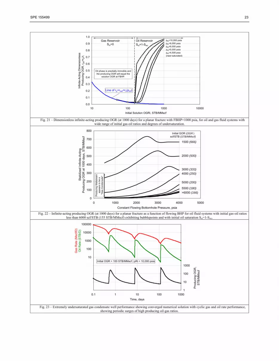
SPE 155499 23

 

0.0

0.1

0.2

0.3

0.4

0.5

0.6

0.7

0.8

0.9

1.0

10 100 1000 10000

Initial Solution OGRi, STB/MMscf

Infin

ite-A

ctin

g D

imen

sio

nles

sP

rodu

cin

g O

GR

, rp

D=

r p/r

i

Line of rp=rswf=rs(pwf)

pRi=10,000 psiapRi=8,000 psiapRi=6,000 psiapRi=5,000 psiapRi=4,500 psia(near-saturated)

Gas ReservoirSoi=0

Oil Reservoir

Oil phase is practially immobile and the producing OGR will equal the

solution OGR at FBHP.

Soi=1-Swc

Fig. 21 – Dimensionless infinite-acting producing OGR (at 1000 days) for a planar fracture with FBHP=1000 psia, for oil and gas fluid systems with

wide range of initial gas-oil ratios and degrees of undersaturation.  

0

100

200

300

400

500

600

700

800

0 1000 2000 3000 4000 5000

Constant Flowing Bottomhole Pressure, psia

Sta

bili

zed

Infin

ite-A

ctin

gP

rodu

cin

g O

GR

at 1

000

day

s, S

TB

/MM

scf

Initial GOR (OGR )scf/STB (STB/MMscf)

5000 (200)

4000 (250)

3000 (333)

2000 (500)

1500 (666)

5500 (180)

>6000 (166)

Pro

duci

ng W

ells

trea

map

pea

rs to

be

a"G

as C

ond

ensa

te"

Fig. 22 – Infinite-acting producing OGR (at 1000 days) for a planar fracture as a function of flowing BHP for oil fluid systems with initial gas-oil ratios

less than 6000 scf/STB (155 STB/MMscf) exhibiting bubblepoints and with initial oil saturation Soi=1-Swc.

 

0.001

0.01

0.1

1

10

100

1000

10000

100000

0.1 1 10 100 1000

Time, days

Ga

s R

ate

(M

scf/D

)O

il R

ate

(S

TB

/D)

1

10

100

1000

10000

100000

1000000

10000000

100000000

Pro

duci

ng O

GR

,S

TB

/MM

scf

Initial OGR = 100 STB/MMscf | pRi = 10,000 psia

Fig. 23 – Extremely undersaturated gas condensate well performance showing converged numerical solution with cyclic gas and oil rate performance,

showing periodic surges of high producing oil-gas ratios.

24 SPE 155499

 

1

10

100

1000

0.1 1 10 100 1000

Time, days

Ga

s R

ate

(Msc

f/D)

and

Oil

Ra

te (

ST

B/D

)

1000

10000

100000

1000000

Flo

win

g B

ott

omho

le P

ress

ure,

psi

a

GORi=4,000 scf/STB (250 STB/MMscf) Oil

GORi=6,500 scf/STB (155 STB/MMscf) Critical

GORi=20,000 scf/STB (50 STB/MMscf) Gas

GORi=4,000 scf/STB

GORi=4,000 scf/STB

GORi=4,000 scf/STB

Fig. 24 – Production performance for constant-gas rate of 1 MMscf/D until minimum BHP of 1000 psia is reached, for a range of reservoir fluids from

low-yield gas condensate to critical to high-GOR oil.

 

0

50

100

150

200

250

300

0 1000 2000 3000 4000 5000 6000

Flowing Bottomhole Pressure, psia

Pro

duci

ng O

il-G

as R

atio

, ST

B/M

Msc

f

GORi=4,000 scf/STB (250 STB/MMscf) Oil

GORi=6,500 scf/STB (155 STB/MMscf) Critical

GORi=7,500 scf/STB (133 STB/MMscf) Gas

GORi=10,00 scf/STB (100 STB/MMscf) Gas

GORi=20,000 scf/STB (50 STB/MMscf) Gas

Solution OGR, rs(pwf)

Fig. 25 – Producing OGR versus flowing BHP for constant-gas rate of 1 MMscf/D until minimum BHP of 1000 psia is reached, for a range of reservoir

fluids from low-yield gas condensate to critical to high-GOR oil.  

0.00

0.05

0.10

0.15

0.20

0.25

0.30

0 0.1 0.2 0.3 0.4 0.5 0.6 0.7 0.8 0.9

Sgi

Dim

ensi

onle

ss P

rodu

cing

OG

R, r

pD=

r p/r

i

Infin

ite-A

ctin

g P

erio

d

OilReservoir

Gas CondensateReservoir

Saturated Two-Phase Gas-Oil Initial Reservoir

Fig. 26 – Dimensionless producing OGR for a saturated one- and two-phase LRS well producing against a constant FBHP of 1000 psia with a 1D

planar fracture model, showing the impact of stabilized infinite-acting OGR variation with the initial gas saturation in the reservoir.

SPE 155499 25

 

1

10

100

1000

0.1 1 10 100 1000

Time, days

Gas

Rat

e (M

scf/D

) an

d O

il R

ate

(ST

B/D

)

1000

10000

100000

1000000

Flo

win

g B

otto

mho

le P

ress

ure,

psi

a

Sgi=0%

Sgi=0%

Sgi=10%

Sgi=30%

Sgi=60%

Sgi=0%

Fig. 27 – Production performance for a well producing with 1 MMscf/D until pwf=1000 psia is reached. Reservoir fluid systems are studied for pRi=3500

psia, for saturated oil (Sgi =0) and a range of two-phase saturated systems with varying Sgi.

 

0

50

100

150

200

250

300

350

400

450

500

0 1000 2000 3000 4000 5000 6000

Flowing Bottomhole Pressure, psia

Pro

duci

ng O

il-G

as R

atio

, S

TB

/MM

scf

Sgi=0%

Sgi=10%

Sgi=20%

Sgi=30% Solution rs(pwf)

50%

Sgi=40%

Any Sgi≥60% results in producing OGR rp=rs(pwf).

Well goes on decline when FBHP reaches

1000 psia, at which time the richer systems

(Sgi≤20%) show increasing liquid yield with

time, rp(t).

rp(t)

Initial OGRi=460 (Sgi=0%)

Fig. 28 – Producing OGR versus flowing BHP for constant-gas rate of 1 MMscf/D until minimum BHP of 1000 psia is reached, for a range of saturated

reservoir fluid systems at 3500 psia initial reservoir pressure and varying amounts of initial gas saturation.