Quantifying the impact of environmental variables upon catch-per-unit-effort of blue shark Prionace glauca in the western English Channel

Journal of Fish Biology (2014)

doi:10.1111/jfb.12448, available online at wileyonlinelibrary.com

Quantifying the impact of environmental variables uponcatch per unit effort of the blue shark Prionace glauca in the

western English Channel

J. D. Mitchell*†, K. J. Collins*, P. I. Miller‡ and L. A. Suberg*

*National Oceanography Centre, University of Southampton, Waterfront Campus, EuropeanWay, Southampton SO14 3ZH, U.K. and ‡Plymouth Marine Laboratory, Prospect Place, The

Hoe, Plymouth PL1 3DH, U.K.

(Received 17 February 2014, Accepted 15 May 2014)

The effect of environmental variables on blue shark Prionace glauca catch per unit effort (CPUE) ina recreational fishery in the western English Channel, between June and September 1998–2011, wasquantified using generalized additive models (GAMs). Sea surface temperature (SST) explained 1⋅4%of GAM deviance, and highest CPUE occurred at 16⋅7∘ C, reflecting the optimal thermal preferencesof this species. Surface chlorophyll a concentration (CHL) significantly affected CPUE and caused27⋅5% of GAM deviance. Additionally, increasing CHL led to rising CPUE, probably due to higherproductivity supporting greater prey biomass. The density of shelf-sea tidal mixing fronts explained 5%of GAM deviance, but was non-significant, with increasing front density negatively affecting CPUE.Time-lagged frontal density significantly affected CPUE, however, causing 12⋅6% of the deviancein a second GAM and displayed a positive correlation. This outcome suggested a delay between theevolution of frontal features and the subsequent accumulation of productivity and attraction of highertrophic level predators, such as P. glauca.

© 2014 The Fisheries Society of the British Isles

Key words: environmental preferences; fisheries management; generalized additive model; recre-ational fishery.

INTRODUCTION

The blue shark Prionace glauca (L. 1758) is a pelagic predator of the family Car-charhinidae (Compagno, 1984) that undertakes extensive migratory movementsthroughout the North Atlantic Ocean (Kohler et al., 1998; Fitzmaurice et al., 2005). Inthe eastern North Atlantic, sharks remain in the western English Channel and CelticSea between June and October (Vas, 1990), before moving south-west through the Bayof Biscay and past the Iberian Peninsula (Stevens, 1976, 1990). Marked age and sexsegregation occur within this North Atlantic population (Kohler et al., 1998; Nakano& Stevens, 2009), with female dominance in the western English Channel reflectedby sex ratios of 3⋅2:1 (Stevens, 1976) and 9⋅4:1 females:male (J. D. Mitchell &

†Author to whom correspondence should be addressed at present address: 2 Whitmore Road, Taunton, SomersetTA2 6DY, U.K. Tel.: +44 7917 322413; email: [email protected]

1

© 2014 The Fisheries Society of the British Isles

2 J . D . M I T C H E L L E T A L.

K. J. Collins, unpubl. data). Prionace glauca found in this area are also predominantlyjuvenile or sub-adult life stages (Stevens, 1976, 1990), as classified by total lengths(LT) of <173 and 173–221 cm for females of these respective categories in the NorthAtlantic population (Pratt, 1979). Stevens (1976) recorded a maximum LT of 220cm from c. 950 P. glauca measured in the western English Channel, indicating anabsence of mature P. glauca, and recent data from 1998 to 2011 also showed onlyc. 10% of c. 1100 measured P. glauca to be mature (J. D. Mitchell & K. J. Collins,unpubl. data).

Migratory movements of P. glauca are primarily driven by water temperature andprey availability (Vas, 1990; Nakano & Seki, 2003). Summer movements to higherlatitudes are facilitated by warming seas, with the theoretical optimal thermal rangeof P. glauca, which is between 13 and 18∘ C in the North Atlantic Ocean (Casey,1982), probably determining the time of arrival and duration of residency in the west-ern English Channel (Vas, 1990). Highly productive areas such as those supported byoceanographic fronts are known to strongly influence predatory pelagic fish distribu-tion, including that of swordfish Xiphias gladius L. 1758 (Podestá et al., 1993), tunas(Fiedler & Bernard, 1987; Royer et al., 2004) and P. glauca (Queiroz et al., 2010).Therefore, the opportunity to feed in highly productive shelf waters of the westernEnglish Channel, where tidal mixing fronts and phytoplankton blooms concentrate pro-ductivity in summer months (Pingree et al., 1975; Miller, 2004; Garcia-Soto & Pingree,2009; Smyth et al., 2010), supporting large schools of clupeids and Atlantic mackerelScomber scombrus L. 1758 (Southward et al., 2004), key prey species of P. glauca(Stevens, 1973; Compagno et al., 2005), is likely to be a significant factor attract-ing them to this region. Indeed, Vas (1990) identified a numerical correlation betweenAtlantic herring Clupea harengus L. 1758 and European pilchard Sardina pilchardus(Walbaum 1792) abundance, and that of P. glauca, in this area. Additionally, produc-tive fronts in the western English Channel markedly affect the distribution of otherlarge pelagic fish, such as basking sharks Cetorhinus maximus (Gunnerus 1765) (Sims& Quayle, 1998) and ocean sunfish Mola mola (L. 1758) (Sims & Southall, 2002), andhigh productivity associated with fronts had a significant positive effect on P. glaucadistribution in the nearby Celtic Sea (Queiroz et al., 2012).

Sea temperature, productivity and the presence of fronts would also be expected toaffect catch per unit effort (CPUE) of P. glauca in this region, due to the probabilityof higher abundance and residence times of P. glauca in areas with optimal environ-mental conditions. This research sought to quantify these potential interactions in arecreational fishery between June and September 1998–2011 by using generalizedadditive models (GAMs) (Hastie & Tibshirani, 1986) [Venables & Dichmont (2004)provide an overview of GAMs in fisheries science].

Whilst the effect of environmental variables on P. glauca CPUE has been investigatedusing GAMs in open-ocean commercial fisheries in the North Pacific Ocean (Bigelowet al., 1999; Walsh & Kleiber, 2001) and South Atlantic Ocean (Carvalho et al., 2011),it has not been analysed in the North Atlantic Ocean or in productive shelf waters suchas those of the western English Channel. This study therefore offered the potentialfor increasing ecological understanding of this species, particularly its environmentalpreferences and vulnerability to fisheries in this region. Furthermore, this study quan-tifies these relationships for mostly juvenile and sub-adult female P. glauca; thus, itcan be compared with data from other studies (Bigelow et al., 1999; Walsh & Kleiber,2001; Carvalho et al., 2011) on different populations and life stages to identify sex and

© 2014 The Fisheries Society of the British Isles, Journal of Fish Biology 2014, doi:10.1111/jfb.12448

P R I O NAC E G L AU C A C P U E I N T H E E N G L I S H C H A N N E L 3

age variation in ecological dynamics. This information is vital for creating effectivefisheries management models, such as those which could use ecological informationand environmental data alongside P. glauca movements to identify important aggre-gation areas to protect from fishing pressure. Management is needed because of thehuge and potentially unsustainable commercial harvest of the North Atlantic popula-tion for fins (Baum et al., 2003), a process that occurs through by-catch in X. gladiusand tuna longline fisheries (Buencuerpo et al., 1998; Clarke et al., 2006; Nakano &Stevens, 2009), and in some targeted fisheries (Aires-da-Silva et al., 2009). Indeed,North Atlantic commercial landings of P. glauca increased from 3028 t in 1990 to 37178 t in 2010 (ICCAT, 2012), with most standardized abundance indices indicatingcontinual declines in recent decades (Simpfendorfer et al., 2002; Baum et al., 2003;Campana et al., 2006; Aires-da-Silva et al., 2008).

MATERIALS AND METHODS

S T U DY L O C AT I O N A N D F I S H E RYThis study was conducted in the western English Channel where the Shark Angling Club

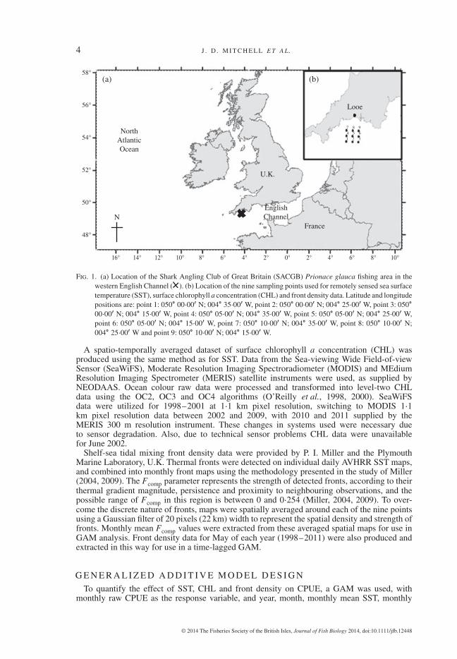
of Great Britain (SACGB) recreational fishery targets P. glauca between June and September[Fig. 1(a)]. The area of fishing operations is 16–40 km south of the port of Looe, Cornwall, andcovers an area of c. 500 km2. The SACGB began as a catch and kill enterprise in 1952 (Caunter,1961), and is currently composed of six charter vessels which catch c. 200–600 sharks annually.All anglers now practise catch and release, and sharks are measured for LT and mass beforebeing tagged and released. Tag and measurement data are supplied to and collated by the U.K.Shark Tagging Programme. Fishing is conducted in an area of sandy substratum with depths of70–80 m. On arrival at a fishing location, mesh chum bags are deployed over the side of thevessel, containing fish chunks, oil and blood to attract sharks. Between four and 10 rods baitedwith whole S. scombrus are set in this odour trail, with hooks at varying depths and distancesfrom the vessel. J-hooks of sizes 12/0 and 10/0 are widely used, with 9–45 kg (20–100 lb)monofilament line attached to the hook via a wire trace, which prevents sharks breaking theline. Fishing time is typically between 5 and 7 h.

R AW C P U E DATARaw CPUE data from the SACGB fishery log included number of charter vessel trips run and

number of P. glauca caught on a daily basis between June and September 1998–2011. Thisrecord allowed creation of a monthly raw CPUE index, in the form of total monthly P. glaucacaught per total number of monthly charter vessel trips. Unfortunately, data from the SACGBfishery log did not reliably record the number of hooks used or the overall fishing time of eachtrip, preventing these more detailed units of effort being available for creation of the CPUEindex.

E N V I RO N M E N TA L DATASea surface temperature (SST) data for June to September 1998–2011 were obtained from the

advanced very high resolution radiometer (AVHRR). These data were collected by the NaturalEnvironment Research Council (NERC) Earth Observation Data Acquisition and Analysis Ser-vice (NEODAAS). Calibrated level-two SST data, collected and processed by the Panorama sys-tem (Miller et al., 1997), were spatially averaged over the SACGB fishing area, and temporallyaveraged over monthly periods. This involved collecting cloud-free SST data as often as possi-ble for a grid of nine discrete latitude and longitude positions [Fig. 1(b)] equidistantly spacedthroughout the fishing area, and generating an overall mean SST value for all nine points overeach month. SST data for each latitude and longitude point represented a pixel area of 1⋅21 km2.



(a)

NorthAtlanticOcean

(b)

16° 14° 12° 10° 8° 6° 4° 2° 0° 2° 4°

EnglishChannel

France

U.K.

Looe

6° 8° 10°

48°

50°

52°

54°

56°

58°

7 8

4

1 2 3

5 6

9

N

Fig. 1. (a) Location of the Shark Angling Club of Great Britain (SACGB) Prionace glauca fishing area in thewestern English Channel ( ). (b) Location of the nine sampling points used for remotely sensed sea surfacetemperature (SST), surface chlorophyll a concentration (CHL) and front density data. Latitude and longitudepositions are: point 1: 050∘ 00⋅00′ N; 004∘ 35⋅00′ W, point 2: 050∘ 00⋅00′ N; 004∘ 25⋅00′ W, point 3: 050∘00⋅00′ N; 004∘ 15⋅00′ W, point 4: 050∘ 05⋅00′ N; 004∘ 35⋅00′ W, point 5: 050∘ 05⋅00′ N; 004∘ 25⋅00′ W,point 6: 050∘ 05⋅00′ N; 004∘ 15⋅00′ W, point 7: 050∘ 10⋅00′ N; 004∘ 35⋅00′ W, point 8: 050∘ 10⋅00′ N;004∘ 25⋅00′ W and point 9: 050∘ 10⋅00′ N; 004∘ 15⋅00′ W.

A spatio-temporally averaged dataset of surface chlorophyll a concentration (CHL) wasproduced using the same method as for SST. Data from the Sea-viewing Wide Field-of-viewSensor (SeaWiFS), Moderate Resolution Imaging Spectroradiometer (MODIS) and MEdiumResolution Imaging Spectrometer (MERIS) satellite instruments were used, as supplied byNEODAAS. Ocean colour raw data were processed and transformed into level-two CHLdata using the OC2, OC3 and OC4 algorithms (O’Reilly et al., 1998, 2000). SeaWiFSdata were utilized for 1998–2001 at 1⋅1 km pixel resolution, switching to MODIS 1⋅1km pixel resolution data between 2002 and 2009, with 2010 and 2011 supplied by theMERIS 300 m resolution instrument. These changes in systems used were necessary dueto sensor degradation. Also, due to technical sensor problems CHL data were unavailablefor June 2002.

Shelf-sea tidal mixing front density data were provided by P. I. Miller and the PlymouthMarine Laboratory, U.K. Thermal fronts were detected on individual daily AVHRR SST maps,and combined into monthly front maps using the methodology presented in the study of Miller(2004, 2009). The Fcomp parameter represents the strength of detected fronts, according to theirthermal gradient magnitude, persistence and proximity to neighbouring observations, and thepossible range of Fcomp in this region is between 0 and 0⋅254 (Miller, 2004, 2009). To over-come the discrete nature of fronts, maps were spatially averaged around each of the nine pointsusing a Gaussian filter of 20 pixels (22 km) width to represent the spatial density and strength offronts. Monthly mean Fcomp values were extracted from these averaged spatial maps for use inGAM analysis. Front density data for May of each year (1998–2011) were also produced andextracted in this way for use in a time-lagged GAM.

G E N E R A L I Z E D A D D I T I V E M O D E L D E S I G N

To quantify the effect of SST, CHL and front density on CPUE, a GAM was used, withmonthly raw CPUE as the response variable, and year, month, monthly mean SST, monthly



mean CHL and monthly mean front density as the predictor variables. Raw CPUE data werelog-normally distributed; therefore, a natural log(ln) transformation was applied to normalizethe data and produce a Gaussian distribution for the GAM. Normality was confirmed by aKolmogorov–Smirnov (K–S) test (D55 = 0⋅11, > 0.05), performed in the software programmeMinitab 16 (Minitab Inc.; www.minitab.com/en-GB/products/minitab/default.aspx). A Gaus-sian model with its natural (canonical) identity link function thus represented the most appro-priate and reliable fit for the transformed CPUE data, compared with other possible GAM errordistributions and link functions. A constant (0⋅1) was added prior to the ln transformation toavoid undefined logarithms resulting from zero CPUE values, a practise which is commonplacewhere CPUE data are analysed in GAMs (Maunder & Punt, 2004). The value of 0⋅1 was chosenover other potential constants as it dealt with zero CPUE values whilst only having minimaleffects on the nature of the data, and because it is a widely used constant applied in other studiesanalysing effects of environmental variables upon CPUE (Bigelow et al., 1999). The expectedrange of CPUE values as a result of this ln transformation and addition of a constant was −1⋅01to 1⋅55, and the ln transformation also meant that all GAM results presented later describe mul-tiplicative effects on CPUE. The GAM was run using the mgcv package (Wood, 2006) in R(2.15.3., The R Foundation for Statistical Computing; www.r-project.org). Environmental pre-dictor variables were smoothed to account for their non-linear, variable nature (Craven & Wabha,1979; Wood, 2008).

GAM robustness was checked by diagnostic procedures, including backward stepwiseselection of the model with lowest residual deviance and confirmation of the independence andnormality of residuals, as well as the GAM goodness-of-fit. Akaike information criteria (AIC)(Akaike, 1974), variance inflation factors (VIFs) and general cross validation (GCV) scoresalso confirmed model robustness (Hastie & Tibshirani, 1986; Wood, 2008; Zuur et al., 2009).The resulting GAM was fitted in the following form: ln(Zi + 0⋅1)= Y +M + s(T , ts = crs)+ s(C,ts = crs)+ s(D, ts = crs), where Z =monthly raw CPUE, i= identity link function, Y = year,M =month, s= smoothed predictor variable, T =monthly mean SST, ts = type of smoothing,crs = cubic regression spline smoothing, C =mean monthly CHL and D=monthly mean frontdensity. Cubic regression spline smoothing was selected over other smoothing types as itproduced the most robust GAM with lowest residual deviance and GCV values (Wood, 2008).Year and month were included as they were likely to account for substantial variation in CPUEover the 14 year dataset. The per cent deviance in the response variable caused by each ofthe predictors, their significance as identified by F tests and the overall per cent deviance wasquantified by adding each variable in a forward stepwise process. The specific, independenteffect of SST, CHL and front density on transformed monthly raw CPUE, across the range ofvalues that occurred for these variables during June to September 1998–2011, was modelledby the GAM and visualized with plots.

A second GAM was also run to analyse the effect of time-lagged front density upon trans-formed CPUE. This model used identical data and the same structure as the original GAM,apart from which it analysed the relationship between monthly CPUE values and the previousmonth’s front density value (i.e. a time lag of 1 month), including that of May each year, asopposed to the same month’s front density value in the original non-time-lagged GAM. Plots ofthis relationship were also created using the technique detailed previously. This enabled directcomparison between time-lagged and non-time-lagged effects of front density on transformedCPUE. Diagnostic procedures were run for the second model, as in the original GAM, confirm-ing its robustness.

RESULTS

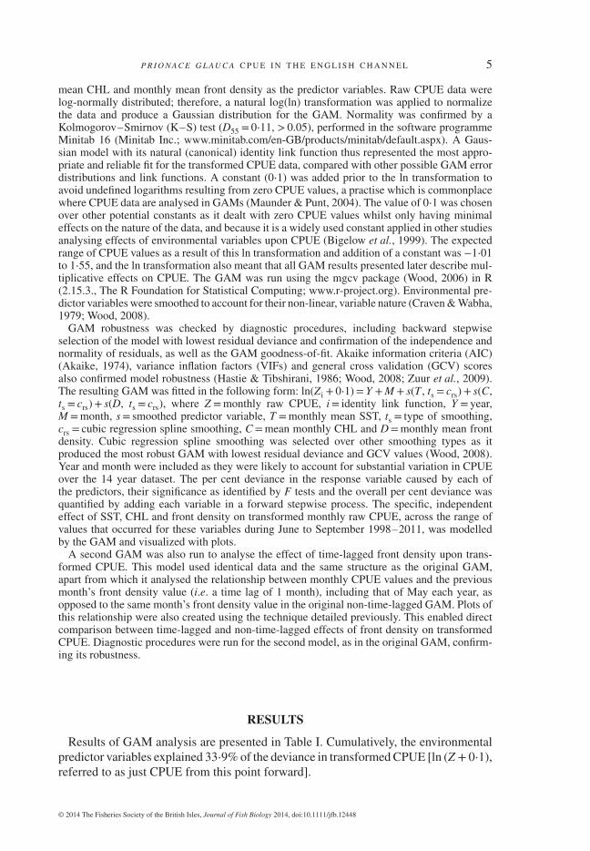
Results of GAM analysis are presented in Table I. Cumulatively, the environmentalpredictor variables explained 33⋅9% of the deviance in transformed CPUE [ln (Z + 0⋅1),referred to as just CPUE from this point forward].



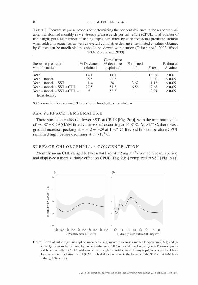
Table I. Forward stepwise process for determining the per cent deviance in the response vari-able, transformed monthly raw Prionace glauca catch per unit effort (CPUE, total number offish caught per total number of fishing trips), explained by each individual predictor variablewhen added in sequence, as well as overall cumulative deviance. Estimated P values obtainedby F tests can be unreliable, thus should be viewed with caution (Guisan et al., 2002; Wood,

2006; Zuur et al., 2009)

Stepwise predictorvariable added

% Devianceexplained

Cumulative% devianceexplained

Estimatedd.f. F-test

EstimatedP value

Year 14⋅1 14⋅1 1 13⋅97 < 0⋅01Year+month 8⋅5 22⋅6 1 0⋅02 > 0⋅05Year+month+ SST 1⋅4 24 3⋅62 1⋅16 > 0⋅05Year+month+ SST+CHL 27⋅5 51⋅5 6⋅56 2⋅63 < 0⋅05Year+month+ SST+CHL+

front density5 56⋅5 1 3⋅94 < 0⋅05

SST, sea surface temperature; CHL, surface chlorophyll a concentration.

S E A S U R FAC E T E M P E R AT U R E

There was a clear effect of lower SST on CPUE [Fig. 2(a)], with the minimum valueof −0⋅87± 0⋅29 (GAM fitted value± s.e.) occurring at 14⋅8∘ C. At >15∘ C, there was agradual increase, peaking at −0⋅12± 0⋅29 at 16⋅7∘ C. Beyond this temperature CPUEremained high, before declining at c. >17∘ C.

S U R FAC E C H L O RO P H Y L L A C O N C E N T R AT I O N

Monthly mean CHL ranged between 0⋅41 and 4⋅22 mg m−3 over the research period,and displayed a more variable effect on CPUE [Fig. 2(b)] compared to SST [Fig. 2(a)],

14·0

–2

–1

0

ln(m

onth

ly r

aw C

PUE

+ 0

·1)

1

2

(a)

14·5 15·0 15·5 16·0

s [Monthly mean SST (°C)]

16·5 17·0 17·5 18·0 18·5 0·5 1·0 1·5 2·0 2·5 3·0 3·5 4·0

(b)

s [Monthly mean surface CHL (mg m–3)]

Fig. 2. Effect of cubic regression spline smoothed (s) (a) monthly mean sea surface temperature (SST) and (b)monthly mean surface chlorophyll a concentration (CHL) on transformed monthly raw Prionace glaucacatch per unit effort (CPUE, total number fish caught per total number fishing trips), as analysed and fittedby a generalized additive model (GAM). Shaded area represents the bounds of the 95% c.i. (GAM fittedvalue ± 1⋅96 × s.e.).



0·001

–2

–1

0

ln(m

onth

ly r

aw C

PUE

+ 0

·1) 1

2

(a)

0·004 0·008

s [Monthly mean front density (Fcomp)]

0·012 0·016 0·001

(b)

0·004 0·008

s [Monthly mean front density (previous month) (Fcomp)]

0·012 0·016

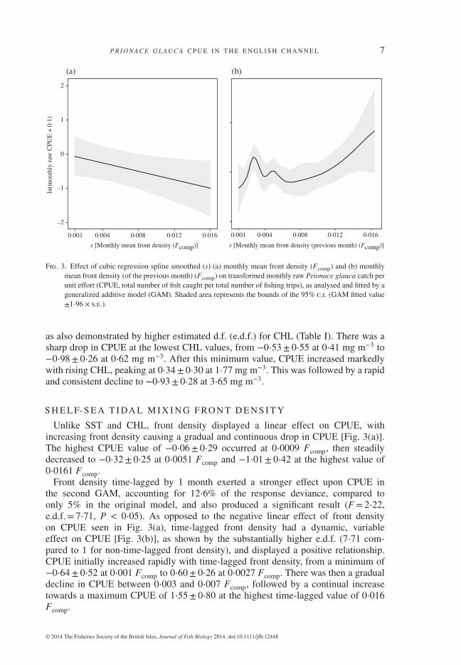
Fig. 3. Effect of cubic regression spline smoothed (s) (a) monthly mean front density (Fcomp) and (b) monthlymean front density (of the previous month) (Fcomp) on transformed monthly raw Prionace glauca catch perunit effort (CPUE, total number of fish caught per total number of fishing trips), as analysed and fitted by ageneralized additive model (GAM). Shaded area represents the bounds of the 95% c.i. (GAM fitted value±1⋅96 × s.e.).

as also demonstrated by higher estimated d.f. (e.d.f.) for CHL (Table I). There was asharp drop in CPUE at the lowest CHL values, from −0⋅53± 0⋅55 at 0⋅41 mg m−3 to−0⋅98± 0⋅26 at 0⋅62 mg m−3. After this minimum value, CPUE increased markedlywith rising CHL, peaking at 0⋅34± 0⋅30 at 1⋅77 mg m−3. This was followed by a rapidand consistent decline to −0⋅93± 0⋅28 at 3⋅65 mg m−3.

S H E L F- S E A T I DA L M I X I N G F RO N T D E N S I T Y

Unlike SST and CHL, front density displayed a linear effect on CPUE, withincreasing front density causing a gradual and continuous drop in CPUE [Fig. 3(a)].The highest CPUE value of −0⋅06± 0⋅29 occurred at 0⋅0009 Fcomp, then steadilydecreased to −0⋅32± 0⋅25 at 0⋅0051 Fcomp and −1⋅01± 0⋅42 at the highest value of0⋅0161 Fcomp.

Front density time-lagged by 1 month exerted a stronger effect upon CPUE inthe second GAM, accounting for 12⋅6% of the response deviance, compared toonly 5% in the original model, and also produced a significant result (F = 2⋅22,e.d.f.= 7⋅71, P < 0⋅05). As opposed to the negative linear effect of front densityon CPUE seen in Fig. 3(a), time-lagged front density had a dynamic, variableeffect on CPUE [Fig. 3(b)], as shown by the substantially higher e.d.f. (7⋅71 com-pared to 1 for non-time-lagged front density), and displayed a positive relationship.CPUE initially increased rapidly with time-lagged front density, from a minimum of−0⋅64± 0⋅52 at 0⋅001 Fcomp to 0⋅60± 0⋅26 at 0⋅0027 Fcomp. There was then a gradualdecline in CPUE between 0⋅003 and 0⋅007 Fcomp, followed by a continual increasetowards a maximum CPUE of 1⋅55± 0⋅80 at the highest time-lagged value of 0⋅016Fcomp.



DISCUSSION

S E A S U R FAC E T E M P E R AT U R E

The minimal, non-significant effect of SST on P. glauca CPUE in the GAM wasunexpected, given the fact that temperature exerts a fundamental effect on the metabolicscope of fishes (Fry, 1971), including the poikilothermic P. glauca. Also, Carvalhoet al. (2011) recorded significant effects of this environmental variable upon CPUE,with SST explaining 9% of GAM deviance for P. glauca commercial CPUE in thesouth-west Atlantic Ocean. A potential reason for the non-significant effect of SST onCPUE observed in this study may be that temperature remained between 13 and 18∘ C,the optimal range of P. glauca in the North Atlantic Ocean (Casey, 1982), throughoutthe water column during June to September when the fishery operated. Thus, if tem-peratures were constantly within this optimal range then it is unlikely that SST wouldexert a variable or significant effect on CPUE, with productivity and front density likelyto be more important.

Peak CPUE occurred at 16⋅7∘ C SST, approximately half-way between the 13 and18 ∘C optimal thermal range proposed by Casey (1982), and Bigelow et al. (1999)and Walsh & Kleiber (2001) also observed peak CPUE levels at c. 16∘ C SST for P.glauca in the Hawaiian X. gladius longline fishery. In addition, Nakano et al. (1985)recorded highest P. glauca CPUE between 14 and 18∘ C in the North Pacific Ocean,and Carvalho et al. (2011) observed a dome-shaped response of CPUE to SST, peakingbetween 16 and 17∘ C in the South Atlantic tuna longline fishery. Furthermore, theseprevious studies also reflected declining CPUE either side of this peak, as does thisstudy, a trend that may have occurred because where SST approaches either end ofthe 13–18∘ C range, the temperature tolerances of P. glauca become more marginal,causing a shift in distribution and a decline in CPUE. These similar results in bothlarge-scale commercial longline fisheries in open-ocean areas, as well as in a smallrecreational fishery conducted in shelf waters in this study, with both catching differ-ent P. glauca populations, suggest that the proposed 13–18∘ C optimum thermal rangefor this species is accurate. Additionally, tracking data recorded by Sciarrotta & Nel-son (1977) in the north-east Pacific Ocean indicated that although P. glauca ranged inwaters between 8⋅5 and 17⋅5∘ C, they spent 73% of their time between 14 and 16∘ C,highlighting this optimal thermal preference. Research by Stevens et al. (2010) alsosuggests a similar, but slightly higher temperature preference of P. glauca in southernhemisphere waters off eastern Australia, where tagged P. glauca spent the majority oftheir time in water between 17 and 20∘ C.

S U R FAC E C H L O RO P H Y L L A C O N C E N T R AT I O N

The significant effect of CHL upon CPUE, along with the high proportion of per centdeviance it explained, was an expected result given the strong link between productiv-ity and biomass of planktivorous prey fishes in this region (Southward et al., 2004;Garcia-Soto & Pingree, 2009). The need to locate patchy, ephemeral prey resourcesis a key factor driving the movements of pelagic apex predators, including P. glauca(Sims et al., 2006; Weng et al., 2008); hence, this influence on P. glauca distributionis likely to be reflected in CPUE. Carvalho et al. (2011) also observed a significanteffect of CHL on P. glauca CPUE in the South Atlantic Ocean, explaining 8% ofGAM deviance. Additionally, Queiroz et al. (2012) recorded increased residence time



and abundance of satellite-tagged P. glauca in discrete, highly productive areas of theCeltic Sea.

The positive relationship between CHL and CPUE observed at lower CHL levelsin this study, with peak CPUE occurring at 1⋅77 mg m−3, reflected results observedby Carvalho et al. (2011), with a similar peak of 2⋅10 mg m−3 recorded. There was amarked decline at higher CHL levels, however, an unexpected result given the previ-ously mentioned importance of productivity to prey abundance and P. glauca distri-bution. The underlying cause of this result may have been data related, because thesubstantially higher error levels towards the higher end of the CHL range indicated thelower reliability of the model fitted relationship between CHL and CPUE, primarilydue to fewer data points. Additionally, these higher monthly mean CHL results wereoften strongly influenced by isolated, vastly higher individual values caused by blooms.These results may have strongly affected the mean, causing it to be skewed and unreal-istically high, probably misrepresenting the true spatio-temporally averaged CHL levelfor certain months. This, in turn, may have produced unreliable results for the modelledCPUE and CHL relationship.

S H E L F- S E A T I DA L M I X I N G F RO N T D E N S I T Y

Due to the ability of tidal mixing fronts to support high productivity (Olson & Backus,1985) and dense biomass of planktivorous prey fishes (Sommer et al., 2002), P. glaucaCPUE would be expected to be positively related to front density. This relationshipwas recorded for P. glauca in the North Pacific Ocean by Bigelow et al. (1999), whoobserved a positive effect of thermal front strength upon CPUE of P. glauca usingGAMs. Likewise, the distribution and residence time of P. glauca in certain areas of theCeltic Sea and Bay of Biscay displayed a significant positive relationship with the pres-ence of fronts (Queiroz et al., 2012). Front density only had a minimal, non-significanteffect on CPUE in the current research, however, and the relationship was opposite tothat expected, with front density having a negative linear effect on CPUE. This trendmay have been caused by a number of underlying factors. Firstly, the high productivityof shelf waters in the western English Channel during summer months (Garcia-Soto& Pingree, 2009; Smyth et al., 2010) will probably support a plentiful abundance ofprey resources across a wide area, not just at small-scale tidal mixing fronts. As aresult, highly mobile P. glauca may not be specifically attracted to and remain res-ident at these discrete fronts, as they would be in open-ocean areas where oceano-graphic fronts act as a distinct and reliable hot-spot for prey in an otherwise food-scarceenvironment (Humphries et al., 2010). Furthermore, the physical differences betweenephemeral tidal mixing fronts around 10–100 km in scale that occur where stratifieddeeper water meets well-mixed shallower water in the western English Channel (Pin-gree et al., 1975; Miller, 2004, 2009), compared to larger (100–1000 km) long-termoceanographic fronts created by convergence of colder subarctic and warmer subtropi-cal water masses in the North Pacific transition zone (NPTZ) (Roden, 1980), probablypresent differing levels of attractiveness to apex predators such as P. glauca. Thismay explain the fact that a positive relationship between front energy and CPUE wasobserved by Bigelow et al. (1999) in fronts of the NPTZ, but not in the uniformlyproductive shelf waters of the western English Channel in the current research.



Another possibility is that the abundance, distribution and thus CPUE of P. glaucawas positively affected by the density of fronts, even in the uniformly productive west-ern English Channel, but this link included a time-lagged effect that may not have beencaptured by the original GAM. Indeed, results from the second GAM recorded a signif-icant and positive effect of 1 month time-lagged front density upon CPUE. This resultsuggested that front density only affected CPUE after a certain time period had elapsed,perhaps due to a delay between the front evolving and its subsequent accumulation ofphytoplankton biomass, followed by attraction of primary and secondary consumersand eventually tertiary predators such as P. glauca. This possibility is reflected byBigelow et al. (1999), who analysed the relationship between front energy and CPUEat time lags of 1 week and 1 month, recording that increasing energy in evolving frontsled to higher P. glauca CPUE. The fitted model for the relationship between this vari-able and CPUE was less accurate or robust at higher levels, due to fewer available datapoints as indicated by larger 95% c.i.; hence, the results should be viewed with caution.

A D D I T I O NA L FAC T O R S A F F E C T I N G C P U E

Alongside the 33⋅9% of deviance in CPUE caused by environmental variables, thefactors year and month also explained a substantial proportion of deviance, possiblydue to changing abundance or distribution of P. glauca over the study period. Factorsnot included in GAM analysis may also have influenced CPUE, especially interannualvariation in abundance of key prey species such as C. harengus and S. pilchardus,which are known to fluctuate widely in the western English Channel (Southward et al.,1988), often due to periodic changes in the North Atlantic Oscillation (NAO) (Alheit &Hagen, 1997). Likewise, tidal dynamics may have caused variation in the spread of theodour plume from fishing vessels as a result of changing tidal phase and tidal streamstrength. Such changes may thus have affected the likelihood of attracting and catchingsharks, and the area over which this could have occurred. Further work should aim toincorporate such factors into GAM analysis to further understand how the ecology ofP. glauca is affected by biotic and abiotic factors in its environment.

The knowledge gained from this research offers a unique insight into the relationshipof P. glauca with its biotic and abiotic environment in shallow, productive shelf watersof the North Atlantic Ocean, adding to existing knowledge gained from open-oceanregions. Also, this study focused upon predominantly juvenile and sub-adult femalefish [<221 cm LT (Pratt, 1979)] of the North Atlantic population, which are foundin the western English Channel due to age and sex segregation in this population(Kohler et al., 1998; Nakano & Stevens, 2009). The combination of this work withthat of Bigelow et al. (1999), Walsh & Kleiber (2001) and Carvalho et al. (2011), allof which were based over a larger area, conducted on different P. glauca populationsand life stages and on data from commercial fisheries, leads to a broader, moreholistic understanding of how P. glauca responds to its environment, and how it maybe affected by fisheries. Such knowledge holds significant potential for developingeffective fisheries management policies. For example, ecological knowledge couldbe utilized alongside real-time remote sensing data for environmental variables andsatellite tracking information to guide longline fishing away from key P. glaucaaggregation areas. Indeed, recent research by Queiroz et al. (2012) highlights thepotential of this integrated approach for identifying critical habitat and conservationtargets for P. glauca in the North Atlantic Ocean. Given the recorded declines in parts



of the North Atlantic population in recent decades (Simpfendorfer et al., 2002; Baumet al., 2003; Campana et al., 2006; Aires-da-Silva et al., 2008), the implementationof such strategies will be vital for reducing such losses and maintaining a stablepopulation in this ocean basin.

The authors would like to thank the University of Southampton for financial support of thisresearch. Also, thanks go to staff and fishermen of the SACGB for providing CPUE data, andto charter vessel skippers M. Collings, D. Bond and P. Curtis for kindly allowing observation ofthe angling process. Gratitude is expressed to NEODAAS for supplying satellite data. Thanksalso go to C. Trueman for assistance with R and GAM design. Finally, gratitude is extended toE. Brothwell and C. Mitchell for their tireless support during this research.

The authors declare that there were no conflicts of interest for this research.

References

Aires-da-Silva, A. M., Hoey, J. J. & Gallucci, V. F. (2008). A historical index of abundance forthe blue shark (Prionace glauca) in the western North Atlantic. Fisheries Research 92,41–52. doi: 10.1016/j.fishres.2007.12.019

Aires-da-Silva, A. M., Lopes Ferreira, R. & Gil Pereira, J. (2009). Blue shark catch-rate patternsfrom the Portuguese swordfish longline fishery in the Azores. In Sharks of the OpenOcean: Biology, Fisheries and Conservation (Camhi, M. D., Pikitch, E. K. & Babcock,E. A., eds), pp. 230–235. Oxford: Blackwell Publishing Ltd.

Akaike, H. (1974). A new look at the statistical model identification. IEEE Transactions onAutomatic Control 19, 716–723. doi: 10.1109/TAC.1974.1100705

Alheit, J. & Hagen, E. (1997). Long-term climate forcing of European herring and sardine pop-ulations. Fisheries Oceanography 6, 130–139. doi: 10.1046/j.1365-2419.1997.00035.x

Baum, J. K., Myers, R. A., Kehler, D. G., Worm, B., Harley, S. J. & Doherty, P. A. (2003).Collapse and conservation of shark populations in the north-west Atlantic. Science 299,389–392. doi: 10.1126/science.1079777

Bigelow, K. A., Boggs, C. H. & He, X. (1999). Environmental effects on swordfish and blueshark catch rates in the US North Pacific longline fishery. Fisheries Oceanography 8,178–198. doi: 10.1046/j.1365-2419.1999.00105.x

Buencuerpo, V., Rios, S. & Moron, J. (1998). Pelagic sharks associated with the swordfish,Xiphias gladius, fishery in the eastern North Atlantic Ocean and the Strait of Gibraltar.Fishery Bulletin 96, 667–685.

Campana, S. E., Marks, L., Joyce, W. & Kohler, N. E. (2006). Effects of recreational and com-mercial fishing on blue sharks (Prionace glauca) in Atlantic Canada, with inferences onthe North Atlantic population. Canadian Journal of Fisheries and Aquatic Sciences 63,670–682. doi: 10.1139/f05-251

Carvalho, F. C., Murie, D. J., Hazin, F. H. V., Hazin, H. G., Leite-Mourato, B. & Burgess, G. H.(2011). Spatial predictions of blue shark (Prionace glauca) catch rate and catch probabil-ity of juveniles in the south-west Atlantic. ICES Journal of Marine Science 68, 890–900.doi: 10.1093/icesjms/fsr047

Casey, J. G. (1982). The blue shark, Prionace glauca. In Fish Distribution (Grosslein, M. D. &Azarovitz, T. R., eds), pp. 45–48. New York, NY: New York Sea Grant Institute.

Caunter, J. A. L. (1961). Shark Angling at Looe. Looe: Atkinson Brothers.Clarke, S. C., Magnussen, J. E., Abercrombie, D. L., McAllister, M. K. & Shivji, M. (2006).

Identification of shark species composition and proportion in the Hong Kong sharkfin market based on molecular genetics and trade records. Conservation Biology 20,201–211. doi: 10.1111/j.1523-1739.2005.00247.x

Compagno, L. J. V. (1984). FAO Species Catalogue vol. 4, part 2: Sharks of the world. Anannotated and illustrated catalogue of shark species known to date: Carcharhiniformes.FAO Fisheries Synopsis 125.

Compagno, L., Dando, M. & Fowler, S. (2005). Sharks of the World, 1st edn. Princeton, NJ:Princeton University Press.



Craven, P. & Wabha, G. (1979). Smoothing noisy data with spline functions. Numerische Math-ematik 31, 377–403. doi: 10.1007/BF01404567

Fiedler, P. C. & Bernard, H. J. (1987). Tuna aggregation and feeding near fronts observed insatellite imagery. Continental Shelf Research 7, 871–881. doi: 10.1016/0278-4343(87)90003-3

Fitzmaurice, P., Green, P., Keirse, G., Kenny, M. & Clarke, M. (2005). Stock discrimination ofthe blue shark based on Irish tagging data. ICCAT Collective Volume of Scientific Papers58, 1171–1178. Available at http://www.iccat.org/Documents/CVSP/CV058_2005/no_3/CV058031171.pdf

Fry, F. E. J. (1971). The effect of environmental factors on the physiology of fish. In Fish Phys-iology, Vol. VI (Hoar, W. S. & Randall, D. J., eds), pp. 1–98. London: Academic Press.

Garcia-Soto, C. & Pingree, R. D. (2009). Spring and summer blooms of phytoplankton (Sea-WiFS/MODIS) along a ferry line in the Bay of Biscay and western English Channel.Continental Shelf Research 29, 1111–1122. doi: 10.1016/j.csr.2008.12.012

Guisan, A., Edwards, T. C. Jr. & Hastie, T. (2002). Generalised linear and generalised additivemodels in studies of species distributions: setting the scene. Ecological Modelling 157,89–100. doi: 10.1016/S0304-3800(02)00204-1

Hastie, T. & Tibshirani, R. (1986). Generalised additive models. Statistical Science 1, 297–310.doi: 10.1214/ss/1177013604

Humphries, N. E., Queiroz, N., Dyer, J. R. M., Pade, N. G., Musyl, M. K., Schaefer, K. M.,Fuller, D. W., Brunnschweiler, J. M., Doyle, T. K., Houghton, J. D. R., Hays, G. C., Jones,C. S., Noble, L. R., Wearmouth, V. J., Southall, E. J. & Sims, D. W. (2010). Environmentalcontext explains Lévy and Brownian movement patterns of marine predators. Nature 465,1066–1069. doi: 10.1038/nature09116

Kohler, N. E., Casey, J. G. & Turner, P. A. (1998). NMFS cooperative shark tagging program,1962-93: an atlas of shark tag and recapture data. Marine Fisheries Review 60, 1–87.

Maunder, M. N. & Punt, A. E. (2004). Standardizing catch and effort data: a review of recentapproaches. Fisheries Research 70, 141–159. doi: 10.1016/j.fishres.2004.08.002

Miller, P. (2004). Multi-spectral front maps for automatic detection of ocean colour fea-tures from SeaWiFS. International Journal of Remote Sensing 25, 1437–1442.doi: 10.1080/01431160310001592409

Miller, P. (2009). Composite front maps for improved visibility of dynamic sea-surface fea-tures on cloudy SeaWiFS and AVHRR data. Journal of Marine Systems 78, 327–336.doi: 10.1016/j.jmarsys.2008.11.019

Miller, P., Groom, S., McManus, A., Selley, J. & Mironnet, N. (1997). Panorama: asemi-automated AVHRR and CZCS system for observation of coastal and oceanprocesses. In RSS97: Observations and Interactions, Proceedings of the 23rd AnnualConference and Exhibition of the Remote Sensing Society (Griffiths, G. & Pearson, D.,eds) Remote Sensing Society, pp. 539–544. Reading: Remote Sensing Society.

Nakano, H. & Seki, M. P. (2003). Synopsis of biological data on the blue shark, (Prionace glaucaLinnaeus). Bulletin of the Fisheries Research Agency of Japan 6, 18–55.

Nakano, H. & Stevens, J. D. (2009). The biology and ecology of the blue shark, Prionace glauca.In Sharks of the Open Ocean: Biology, Fisheries and Conservation (Camhi, M. D., Pik-itch, E. K. & Babcock, E. A., eds), pp. 140–151. Oxford: Blackwell Publishing Ltd.

Nakano, H., Makihara, M. & Shimazaki, K. (1985). Distribution and biological characteristicsof blue shark in the central North Pacific. Bulletin of the Faculty of Fisheries HokkaidoUniversity 36, 99–113.

Olson, D. B. & Backus, R. H. (1985). The concentrating of organisms at fronts: a cold-waterfish and a warm-core Gulf Stream ring. Journal of Marine Research 43, 113–137.

O’Reilly, J. E., Maritorena, S., Mitchell, B. G., Siegel, D. A., Carder, K. L., Garver, S. A.,Kahru, M. & McClain, C. R. (1998). Ocean colour algorithms for SeaWiFS. Journal ofGeophysical Research 103, 24937–24953. doi: 10.1029/98JC02160

O’Reilly, J. E., Maritorena, S., Mitchell, B. G., Siegel, D. A. & Carder, K. L. (2000). Oceancolour chlorophyll a algorithms for SeaWiFS, OC2 and OC4: version 4. In SeaWiFSPostlaunch Calibration and Validation Analyses, Part 3 (Reilly, J. E. & Maritorena, S.,eds), pp. 9–23. Greenbelt, MD: NASA Goddard Space Flight Centre.



Pingree, R. D., Pugh, P. R., Holligan, P. M. & Forster, G. R. (1975). Summer phytoplanktonblooms and red tides along tidal fronts in the approaches to the English Channel. Nature258, 672–677. doi: 10.1038/258672a0

Podestá, G. P., Browder, J. A. & Hoey, J. J. (1993). Exploring the association between swordfishcatch rates and thermal fronts on US longline grounds in the western North Atlantic.Continental Shelf Research 13, 253–277. doi: 10.1016/0278-4343(93)90109-B

Pratt, H. W. (1979). Reproduction in the blue shark, Prionace glauca. Fisheries Bulletin 77,445–470.

Queiroz, N., Humphries, N. E., Noble, L. R., Santos, A. M. & Sims, D. W. (2010). Short-termmovements and diving behaviour of satellite-tracked blue sharks Prionace glaucain the northeastern Atlantic Ocean. Marine Ecology Progress Series 406, 265–279.doi: 10.3354/meps08500

Queiroz, N., Humphries, N. E., Noble, L. R., Santos, A. M. & Sims, D. W. (2012). Spatialdynamics and expanded vertical niche of blue sharks in oceanographic fronts reveal habi-tat targets for conservation. PLoS One 7, e32374. doi: 10.1371/journal.pone.0032374

Roden, G. I. (1980). On the subtropical frontal zone north of Hawaii during winter. Journalof Physical Oceanography 10, 342–362. doi: 10.1175/1520-0485(1980)010<0342:OTSFZN>2.0.CO;2

Royer, F., Fromentin, J.-M. & Gaspar, P. (2004). Association between bluefin tuna schools andoceanic features in the western Mediterranean. Marine Ecology Progress Series 269,249–263. doi: 10.3354/meps269249

Sciarrotta, T. C. & Nelson, D. R. (1977). Diel behaviour of the blue shark, Prionace glauca,near Santa Catalina Island, California. Fishery Bulletin 75, 519–528.

Simpfendorfer, C. A., Hueter, R. E., Bergman, U. & Connett, S. M. H. (2002). Results of afishery-independent survey for pelagic sharks in the western North Atlantic, 1977-1994.Fisheries Research 55, 175–192. doi: 10.1016/S0165-7836(01)00288-0

Sims, D. W. & Quayle, V. A. (1998). Selective foraging behaviour of basking sharks on zoo-plankton in a small-scale front. Nature 393, 460–464. doi: 10.1038/30959

Sims, D. W. & Southall, E. J. (2002). Occurrence of ocean sunfish Mola mola near fronts inthe western English Channel. Journal of the Marine Biological Association of the UnitedKingdom 82, 927–928. doi: 10.1017/ S0025315402006409

Sims, D. W., Witt, M. J., Richardson, A. J., Southall, E. J. & Metcalfe, J. D. (2006). Encountersuccess of free-ranging marine predator movements across a dynamic prey landscape.Proceedings of the Royal Society B 273, 1195–1201. doi: 10.1098/rspb.2005.3444

Smyth, T. J., Fishwick, J. R., Al-Moosawi, L., Cummings, D. G., Harris, C., Kitidis, V., Rees,A., Martinez-Vicente, V. & Woodward, E. M. S. (2010). A broad spatio-temporal viewof the western English Channel observatory. Journal of Plankton Research 32, 585–601.doi: 10.1093/plankt/fbp128

Sommer, U., Stibor, H., Katechakis, A., Sommer, F. & Hansen, T. (2002). Pelagic food webconfigurations at different levels of nutrient richness and their implications for the ratiofish production:primary production. Hydrobiologia 484, 11–20. doi: 10.1023/A:1021340601986

Southward, A. J., Boalch, G. T. & Maddock, L. (1988). Fluctuations in the herring and pilchardfisheries of Devon and Cornwall linked to change in climate since the 16th century.Journal of the Marine Biological Association of the United Kingdom 68, 423–445. doi:10.1017/S0025315400043320

Southward, A. J., Langmead, O., Hardman-Mountford, N. J., Aiken, J., Boalch, G. T., Dando,P. R., Genner, M. J., Joint, I., Kendall, M. A., Halliday, N. C., Harris, R. P., Leaper, R.,Mieszkowska, N., Pingree, R. D., Richardson, A. J., Sims, D. W., Smith, T., Walne, A.W. & Hawkins, S. J. (2004). Long-term oceanographic and ecological research in thewestern English Channel. Advances in Marine Biology 47, 1–105. doi: 10.1016/S0065-2881(04)47001-1

Stevens, J. D. (1973). Stomach contents of the blue shark (Prionace glauca L.) off south-westEngland. Journal of the Marine Biological Association of the United Kingdom 53,357–361. doi: 10.1017/S0025315400022323

Stevens, J. D. (1976). First results of shark tagging in the north-east Atlantic 1972-75. Journalof the Marine Biological Association of the United Kingdom 56, 929–937. doi: 10.1017/S002531540002097X



Stevens, J. D. (1990). Further results from a tagging study of pelagic sharks in the north-eastAtlantic. Journal of the Marine Biological Association of the United Kingdom 70,707–720. doi: 10.1017/S0025315400058999

Stevens, J. D., Bradford, R. W. & West, G. J. (2010). Satellite tagging of blue sharks (Pri-onace glauca) and other pelagic sharks off eastern Australia: depth behaviour, temper-ature experience and movements. Marine Biology 157, 575–591. doi: 10.1007/s00227-009-1343-6

Vas, P. (1990). The abundance of the blue shark, Prionace glauca, in the western English Chan-nel. Environmental Biology of Fishes 29, 209–225. doi: 10.1007/BF00002221

Venables, W. N. & Dichmont, C. M. (2004). GLMs, GAMs and GAMMs: an overview of the-ory for applications in fisheries research. Fisheries Research 70, 319–337. doi: 10.1016/j.fishres.2004.08.011

Walsh, W. A. & Kleiber, P. (2001). Generalised additive model and regression tree analysesof blue shark (Prionace glauca) catch rates in the Hawaii-based commercial longlinefishery. Fisheries Research 53, 115–131. doi: 10.1016/S0165-7836(00)00306-4

Weng, K. C., Foley, D. G., Ganong, J. E., Perle, C., Shillinger, G. L. & Block, B. A. (2008).Migration of an upper trophic level predator, the salmon shark, Lamna ditropis,between distant ecoregions. Marine Ecology Progress Series 372, 253–264. doi:10.3354/meps07706

Wood, S. (2006). Generalised Additive Models: An Introduction with R. Boca Raton, FL: Chap-man & Hall/CRC.

Wood, S. (2008). Fast stable direct fitting and smoothness selection for generalised addi-tive models. Journal of the Royal Statistical Society: Series B 70, 495–518. doi:10.1111/j.1467-9868.2007.00646.x

Zuur, A., Ieno, E. N., Walker, N., Saveliev, A. A. & Smith, G. M. (2009). Mixed Effects Modelsand Extensions in Ecology with R. New York, NY: Springer.

Electronic References

ICCAT (2012). ICCAT Report 2010-2011: Executive Summary: Sharks. Available at http://www.iccat.es/Documents/SCRS/ExecSum/SHK_EN.pdf/ (last accessed 12 April 2013).
