~praisal of the Suitability of - NATO STO

~ ..--.*.-,,-., ..

ADVISORY GROUP FOR AEROSPACE RESEARCH & DEVELOPMENT 7 RUE ANCELLE 92200 NEUILLY SUR S W E FRANCE

:hnical Status Review ~praisal of the Suitability of

NORTH ALANllC TREAT( ORGANlZAllON -e-

AGARD-AR-291

ADVISORY GROUP FOR AEROSPACE RESEARCH & DEVELOPMENT 7 R U E A N C E L L E 92200 NEUILLY S U R S E I N E F R A N C E

AGARD ADVISORY REPORT 291

Technical Status Review Appraisal of the Suitability of Turbulence Models in Flow Calculations (Revue Technique - L‘Evaluation de 1’Applicabilite des Modeles de Turbulence dans le Calcul des Ecoulements)

This Advisory Report was prepared at the request of the Fluid Dynamics Panel of AGARD at a Technical Status Review held in Fricdrichshafen, Germany, 26th April 1990.

I

North Atlantic Treaty Organization Organisation du Traite de I’Atlantique Nord

I

The Mission of AGARD

I According to its Charter, the mission of AGAKD is to bring together thc leading personalities of the NATO nations in the fields of science and technology relating to aerospace for the following purposes:

- Recommending effective ways for the member nations to use their research and development capabilities for the common benefit of the NATO community;

- Providing scientific and technical advice and assistance to the Military Committee in the field of aerospace research and development (with particular regard to its military application);

- Continuously stimulating advances in the aerospace sciences relevant to strengthening the common defence posture;

- Improving the co-operation among member nations in aerospace research and development;

- Exchange of scientific and technical information;

- Providing assistance to member nations for the purpose of increasing their scientific and technical potential;

- Rendering scientific and technical assistance, as requested, to other NATO bodies and to member nations in connection with research and development problems in the aerospace field.

The highest authority within AGARD is the National Delegates Board consisting of officially appointed senior representatives from each member nation. The mission of AGARD is carried out through the Panels which are composed of experts appointed

' by the National Delegates, the Consultant and Exchange Programme and the Aerospace Applications Studies Programme. The results of AGARD work are reported to the member nations and the NATO Authorities through the AGARD series of publications of which this is one.

Participation in AGARD activities is by invitation only and is normally limited to citizens of the NATO nations,

The content of this publication has heen reproduced directly from material supplied by AGARD or the authors.

Published July 1991

Copyright 0 AGARD 199 1 All Rights Reserved

ISBN 92-835-0625- 1

Printed by Speciulised Printing Services Limited 40 Chigwell Lune, Loughton, Essex IGI0 3TZ

Recent Publications of the Fluid Dynamics Panel

AGARDOGRAPHS (AG)

Experimental Techniques in the Field of Low Density Aerodynamics AGARD AG-318 (E),Aprill991

Techniques Experimentales Likes a I’Aerodynamique a Basse Densite AGARD AG-3 18 (FR), April 1990

A Survey of Measurements and Measuring Techniques in Rapidly Distorted Compressible Turbulent Boundary Layers AGARD AG-315, May 1989

Reynolds Number Effects in Transonic Flows AGARD AG-303, December 1988

Three Dimensional Grid Generation for Complex Configurations - Recent Progress AGARD AG-309, March 1988

REPORTS (R)

Aircraft Dynamics at High Angles of Attack Experiments and Modelling AGARD R-776, Special Course Notes, March 1991

Inverse Methods in Airfoil Design for Aeronautical and Turbomachinery Applications AGARD R-780, Special Course Notes, November 1990

Aerodynamics of Rotorcraft AGARD R-781, Special Course Notes, November 1990

Three-Dimensional Supersonic/Hypersonic Flows Including Separation AGARD R-764, Special Course Notes, January 1990

Advances in Cryogenic Wind Tunnel Technology AGARD R-774, Special Course Notes, November 1989

ADVISORY REPORTS (AR)

Rotary-Balance Testing for Aircraft Dynamics AGARD AR-265, Report of WG 11, December 1990

Calculation of 3D Separated Turbulent Flows in Boundary Layer Limit AGARD AR-255, Report of WG10, May 1990

Adaptive Wind Tunnel Walls: Technology and Applications AGARD AR-269, Report of WG12, April 1990

Drag Prediction and Analysis from Computational Fluid Dynamics: State of the Art AGARD AR-256, Technical Status Review, June 1989

CONFERENCE PROCEEDINGS (CP)

Vortex Flow Aerodynamics AGARD CP-494, July 199 1

Missile Aerodynamics AGARD CP-493, October 1990

Aerodynamics of Combat Aircraft Controls and of Ground Effects AGARD CP-465, April 1990

Computational Methods for Aerodynamic Design (Inverse) and Optimization AGARD CP-463, March 1990

Applications of Mesh Generation to Complex 3-D Configurations AGARD CP-464, March 1990

... 111

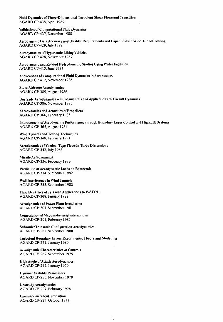
Fluid Dynamics of Three-Dimensional Turbulent Shear Flows and Transition AGARD CP-438, April 1989

Validation of Computational Fluid Dynamics AGARD CP-437, December 1988

Aerodynamic Data Accuracy and Quality: Requirements and Capabilities in Wind Tunnel Testing AGARD CP-429, July 1988

Aerodynamics of Hypersonic Lifting Vehicles AGARD CP-428, November 1987

Aerodynamic and Related Hydrodynamic Studies Using Water Facilities AGARD CP-413, June 1987

Applications of Computational Fluid Dynamics in Aeronautics AGARD CP-4 12, November 1986

Store Airframe Aerodynamics AGARD CP-389, August 1986

Unsteady Aerodynamics - Fundamentals and Applications to Aircraft Dynamics AGARD CP-386, November 1985

Aerodynamics and Acoustics of Propellers AGARD CP-366, February 1985

Improvement of Aerodynamic Performance through Boundary Layer Control and High Lift Systems AGARD CP-365, August 1984

Wind Tunnels and Testing Techniques AGARD CP-348, February 1984

Aerodynamics of Vortical Type Flows in Three Dimensions AGARD CP-342, July 1983

Missile Aerodynamics AGARD CP-336, February 1983

Prediction of Aerodynamic Loads on Rotorcraft AGARD CP-334, September 1982

Wall Interference in Wind Tunnels AGARD CP-335, September 1982

Fluid Dynamics of Jets with Applications to V/STOL AGARD CP-308, January 1982

Aerodynamics of Power Plant Installation AGARD CP-301, September 198 1

Computation of Viscous-Inviscid Interactions AGARD CP-291, February 1981

Subsonic/Transonic Configuration Aerodynamics AGARD CP-285, September 1980

Turbulent Boundary Layers Experiments, Theory and Modelling AGARD CP-27 1, January 1980

Aerodynamic Characteristics of Controls AGARD CP-262, September 1979

High Angle of Attack Aerodynamics AGARD CP-247, January 1979

Dynamic Stability Parameters AGARD CP-235. November 1978

Unsteady Aerodynamics AGARD CP-227, February 1978

Laminar-Turbulent Transition AGARD CP-224, October 1977

iv

Preface

The past decade has seen a rapidly accelerating development of computational methods, following the ever increasing computing power offered by modern technology.

The new tool has found immediate and wide application in fluid dynamics initiating a new era in this field by opening unlimited, as we see it at the present time, horizons in research and development with corresponding technical implications for the aerospace industry. In retrospect it appears, that the fluid dynamicist of the sixties or even the seventies, could have hardly imagined that solving problems of considerable complexity as those handled by today’s computers, could have been possible within the elapsed short period of time.

During the first part of the past decade the ability of the developed computer codes to produce relatively economically a great amount of information regarding flow characteristics around bodies of complex geometries created a sense of euphoria mainly among users of computational techniques. However, it was soon recognized that in order to produce valid answers to questions related to intricate flow cases by employing CFD methods, more is required than simply developing computer capabilities matching the complexities of the problem. Validation procedures, initiated as early as 1968 with the first Stanford conference, have been gradually introduced as an indispensable part of developing valid computer codes. Equally important, it has been also widely recognized, that suitable modelling of physical processes in flows, such as turbulence transport, constitutes a crucial factor for the development of successful prediction codes. This cannot be achieved without adequate understanding of the underlying physical aspects of these phenomena.

The Fluid Dynamics Panel of AGARD has shown a keen interest in computational fluid dynamics in general and for turbulence modelling in particular, following very closely the developments in these areas, as related to the arising needs, especially in the aerospace industry. As a result, several activities in the form of symposia, specialists’ meetings, working groups etc. have been proposed and organized by the panel during the last decade. In this context the FDP has organized a Technical Status Review activity on the “Appraisal of the Suitability of Turbulence Models in Flow Calculations’’ which took place in Friedrichshafen, Germany on April 26, 1990, resulting in the publication of the present Advisory Report. The general scientific scope within which the present TSR activity was placed, has been defined as follows:

i) To carry out an in depth appraisal of the suitability of existing turbulence models for use in flow calculations. For this purpose, available information from the existing theoretical and experimental work on the subject should be reviewed and critically evaluated.

In this process, the underlying physical concepts for each particular turbulence model should be considered as they apply to different flow cases, therefore establishing the range of validity of each model for flow calculations. Existing uncertainties, discrepancies, inadequacies and failures in reported results, rising from inherent limitations in the employed model and/or its inappropriate application, should be pointed out and discussed.

ii) To evaluate the potential of existing knowledge regarding turbulence models, in covering present and future needs in the field of flow calculations.

iii) Based on the above studies, to issue guidelines for future theoretical and experimental work and propose a number of key experiments and flow calculations cases to be conducted in the future.

Since the capability of a Technical Status Review activity to fulfil such an ambitious scope is rather limited, a subcommittee has been initiated and operates, in order to follow developments on the subject and suggest to the panel future appropriate actions to be taken.

As the chairman of the Technical Status Review I would like to express my gratitude to each and all members of the committee responsible for organizing and implementing this activity. Their interest and enthusiasm has guaranteed the participation of well-known members of the scientific community working on the subject. I would also like to express my appreciation to the executive of the Fluid Dynamics Panel, Dr W.Goodrich for the interest he has shown and the assistance extended to the committee in carrying this effort to its final goal of publishing the present Advisory Report.

D.D.Papailiou Chairman of the TSR committee

V

Priiface

1

La dernikre dicennie a it6 marqule par le diveloppement fulgurant des mtthodes de calcul grice h I’accroissement de la puissance des ordinateurs offert par les technologies modernes.

Ce nouvel outil a trouvt des applications diverses et immtdiates en dynamique des fluides, ou il a p e d s d’ouvrir un noveau domaine d’intirit avec, apparemment, des hoGzons illimitts de recherche et dtveloppement ayant des implications techniques importantes pour l’industrie atrospatiale. Rttrospectivement, il est certain que le spicialiste en dynamique des fluides des annies soixante ou soixante dix aurait eu du mal imaginer que la rtsolution de problkmes aussi complexes que ceux qui sont trait& par les ordinateurs modernes serait acquise dans un laps de temps si court.

Pendant la premikre partie de la dernikre dicennie, la capaciti des codes machine Cvoluis pour gtntrer, B faible co0t relatif, un volume considirable de donnies sur les caractiristiques des icoulements autour de corps de gbmttries complexes a crt% I’euphorie, principalement chez les utilisateurs des techniques de calcul. Cependant, il a i t6 vite reconnu que pour obtenir des rtponses valables aux questions touchant des cas d’tcoulements complexes avec des mtthodes d’atrodynamique numkrique, il ne suffit pas seulement de divelopper les capacitks de l‘ordinateur pour qu’il corresponde aux complexitis du problkme.

Les proctdures de validation, dont les premikres datent de 1968, tpoque de la premikre confirence de Stanford, se sont rivtltes peu a peu indispensable au diveloppement de codes machine valables.

II est igalement important de noter qu’il a i t i largement reconnu que la modtlisation adequate de certains processus physiques dans les icoulements, tel que le transport de la turbulence, constitue un facteur critique pour le diveloppement de codes de pridiction performants. Ceci ne peut se faire sans I’acquisition de connaissances appropriies des aspects physiques sous- jacents de ces phtnomknes.

Le Panel AGARD de la dynamique des fluides s’intiresse vivement a I’atrodynamique numerique en giniral et a la modilkation de la turbulence en particulier. I1 suit de trks prks les travaux en cours dans ces domaines, dans la mesure 00 ils correspondent aux besoins qui se font sentir, en particulier dans I‘industrie airospatiale. Par constquent, diffirentes activitis telles que symposia, riunions de spicialistes, groupes de travail etc.. ont 6tt propostes et organisies par le Panel au cours de la dernitre dtcennie. Dans ce cadre, le FDP a diveloppt une activitt de revue technique de M a t de I’art, intitulte “L‘tvaluation de I’applicabilitt de modkles de turbulence dans le calcul des icoulements” le 26 avril 1990 a Friedrichshafen en Allemagne. Le prisent rapport consultatif est le fruit de cette rtunion. Le cadre scientifique gintral de ce rapport est dtfini comme suit:

i) Faire une evaluation detaillie de I’applicabiliti des modkles de turbulence existants pour le calcul des icoulements. A cette fin, les informations rtsultant des travaux thtoriques et expirimentaux doivent itre revus et tvaluts de faGon critique.

Dans ce procidi, les concepts physiques de base pour chaque modele de turbulence doivent itre considiris par rapport a diffirents cas d’tcoulements. Les incertitudes, divergences, insuffisances et Cchecs dont il est fait mention dans les risultats, et qui proviennent des limitations propres du modkle employ6 etlou de son application inopportune doivent itre signalies et discutks.

Evaluer le potentiel des connaissances actuelles en ce qui concerne les modkles de turbulence pour couvrir les besoins actuels et futurs dans le domaine du calcul des Ccoulements.

ii)

iii) Sur la base de ces itudes, Ctablir des directives pour de futurs travaux thtoriques et experimentaux et proposer un certain nombre d‘expiriences clis et de cas de calcul d‘tkoulements B lancer B l’avenir.

Un programme si ambitieux dtborde du cadre d’un tel examen et un sous-comitt a donc CtC crie. I1 a pour mandat de suivre les diveloppements d b s ce domaine et de recommander des actions futures ii prendre par le Panel.

En tant que President de cette revue technique de l’itat de I’art, je tiens B exprimer ma reconnaissance envers tout et chacun des membres du comitt responsable de I’organisation et de la mise en oeuvre de cette activiti. Grice P leur motivation et B leur enthousiasme, nous avons pu compter sur la participation de plusieurs membres iminents de la communautk scientifique qui travaillent sur ce sujet. Je tiens enfin a remercier I’Administrateur du Panel de la Dynamique des Fluides, le Dr W.Goodrich, pour I’inttrit qu’il a manifest6 pour ce project et pour I’aide qu’il a bien voulu apporter au comiti pour la concrktisation de ces efforts sous la forme du prisent rapport consultatif.

D.D. Papailiou

vi

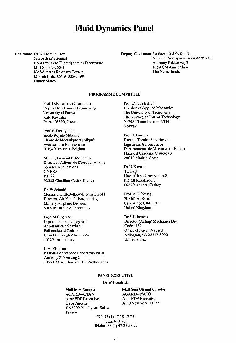
Fluid Dynamics Panel

I Chairman: Dr W.J.McCroskey I Senior Staff Scientist

US Army Aero Flightdynamics Directorate Mail Stop N-258-1 NASA Ames Research Center Moffett Field, CA 94035-1099 United States

I ~

Deputy Chairman: Professor Ir J.W. Slooff National Aerospace Laboratory NLR Anthony Fokkerweg 2 1059 CM Amsterdam The Netherlands

PROGRAMME COMMITTEE

Prof. D. Papailiou (Chairman) Dept. of Mechanical Engineering University of Patras Kat0 Kostritsi Patras 26500, Greece

Prof. R. Decuypere Ecole Royale Militaire Chaire de Mtcanique Appliqute Avenue de la Renaissance B-1040 Brussels, Belgium

M. I’Ing. Gtntral B. Monnerie Directeur Adjoint de I’ACrodynamique pour les Applications ONER4 B.P. 72 92322 Chitillon Cedex, France

Dr. W. Schmidt Messerschmitt-Bolkow-Blohm GmbH Director, Air Vehicle Engineering Military Airplane Division 8000 Munchen 80, Germany

Prof. M.Onorato Dipartimento di Ingegneria Aeronautica e Spaziale Politecnico di Torino C. so Duca degli Abruzzi 24 10129 Torino, Italy

Ir A. Elsenaar National Aerospace Laboratory NLR Anthony Fokkerweg 2 1059 CM Amsterdam, The Netherlands

Prof. Dr T. Ytrehus Division of Applied Mechanics The University of Trondheim The Norwegian Inst. of Technology N-7034 Trondheim - NTH Norway

Prof. J. Jimenez Escuela Tecnica Superior de Ingenieros Aeronauticos Departamento de Mecanica de Fluidos Plaza del Cardenal Cisneros 3 28040 Madrid, Spain

Dr tf.Kaynak TUSA!$ Havacilik ve Uzay San. A.S. P.K. 18 Kavaklidere 06690 Ankara, Turkey

Prof. A.D. Young 70 Gilbert Road Cambridge CB4 3PD United Kingdom

Dr S. Lekoudis Director (Acting) Mechanics Div. Code 1132 Office of Naval Research Arlington, VA 22217-5000 United States

PANEL EXECUTIVE

Dr W. Goodrich

Mail from Europe:

Attn: FDP Executive 7, rue Ancelle F-92200 Neuilly-sur-Seine France

Mail from US and Canada:

Attn: FDP Executive APO New York 00777

AGARD-OTAN AGARD-NATO

Tel: 33 ( 1 ) 47 38 57 75 Telex: 610176F

Telefax: 33 ( I ) 47 38 57 99

vii

Contents

Recent Publications of the Fluid Dynamics Panel

Preface

Prkface

Fluid Dynamics Panel and Programme Committee

Turbulence Modelling: Survey of Activities in Bkigium and the Netherlands, an Appraisal of the Status and a View on the Prospects

_ _ _ _ _ _ __ - * - - - - w ---. -- --- --- by B. van den Berg

JCalculation r- of Turbulent Compressible Flows by J. Cousteix I.___I ---- -*------- -_-___ ___-

/93 G o m e Current Approaches in Turbulence Modelling

UTurbulenee Models for Natural Convection Flows along a Vertical Heated Planc

‘JTurbulent Flow Modelling in Spain. Overview and Developments )

by W. Rodi - r - - - - - __ __c- -. -- - ---_ .T-

-I - - . by D.D. Papailiou

_ _ r -__--_.__. - -- - - - - T I - I-

by C. Dopazo, R. Aliod and L. Valiiio

3 Computational Turbulence Studies in Turkey - --- _- --- --_ r--- --

by U. Kaynak 7

-J Appraisal of the Suitability of Turbulence Models in Flow Calculations: A UK View on Turbulence Models for Turbulent Shear Flow Calculations

Collaborative Testing of Turbulence Models’-l - - .. _ .___ - -- -.

_ _ _ _ _ - -- - - . I - . - _ _ _.__ by G.M. Lilley -c- - -

by P. Bradshaw - , d

Page

iii

V

vi

vii

Reference

1

2

3

4

5

6

7

8

viii

TURBULENCE NODELLING: SWVBY OF ACTIVITIES IN BKLGIM AND THB -S, AN APPRAISAL OF THB STA'KIS AND A VIA3 ON THE PgoSPBCzS

B. van den Berg National Aerospace Lsborstory NIB

P.O. Box 90502 1006 IIW Amaterden The Netherladm

Turbulence research proceeding presently at variou plaaea in the Netherl.nd. and Belgium is briefly reviewed. Subsequently nome experimental results obtained in turbulent boundary layers. as occur on airplane wings, are considered in relation to the

turbulence nodelling in found not to be satisfactory. To support the developnsnt of semi-empirical models of acceptable accuracy. a more extensive base of reliabls turbulence data would be desirable.

USUl tUrbu10nCE model M S W t i O M . ThS Statu Of

constant in mixing length relation mixing length static pressure turbulent kinetic energy fluctuating velocities mean velocities, in x- and y-direction coordinates, approximately para1101 and normal to the mean flow direction boundary layer thickness displacemnt thickness pressure gradient parameter shear atress

Subscripts

e at boundary layer edge tr at transition

at shock w at wall

The need for reasonably accurate turbulence models is becoming more and more pressing due to the progress .ads with the dsvelopant of efficient solution procedures for the Reynolds-averaged Navier- Stokes equations. Though turbulent flow research is being done at many places for quite some time now, progrems has been slow. The field of reasarch is wide and comprises very different flow types, e.g. turbulent boundmy layers along airplane. or ships. atmospheric boundary layers. open water flows. internal flows, f l m with chemical reactions. etc. A P- of the research work going on presently in Belgium and the Natherlanda rill be given here. The main aim of the paper. however, ia to review concisely the state of the art in general and to discuss the proBpects for accurate turbulence model..

After the s 1 1 p a ~ y of local work in section 2, the state of the art in turbulence modelling will be exemplified for a few simple flms in section 3. On the basis of the result. of the brief analysis some conclusion# rill be drew. Finally in section 4 the author'. v i w on the statu and prospects of turbulence modelling will be expressed.

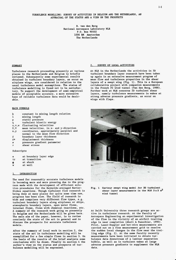
At in the Nstherlenda the activities in 3D turbulent boundary layer research have been taken up again in en extensive measurwnt progru of mean f l m and turbulence properties in the shear layers of a swept wing (Fig. 1). This is a Kuropean collaborative project with companion meuuraments in the French F2 w i n d tunnel (Van den Berg, 1988). Further work at NLR concerns 2D turbulent shear layers, -1y turhulence measurement. in wakes at strong adverse prassure gradients, U occur on wings with flaps.

,' . . -

Fig. 1 Gutmur swept wing model lor SD turbulmt shes= layer measurenents in the NLR 3 x 2 3 rind tyILD.1

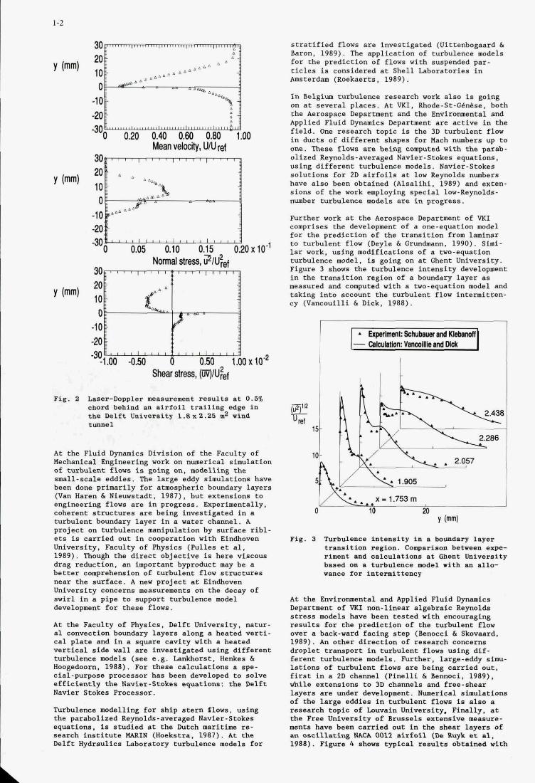
At Delft University three research groups are active in turbulence rasaarch. At the Faculty of Aerospace Engineering an experimental investigation of the f l m in the vicinity of an airfoil trailing edge is near completion (Absil h Passchier, 1990). Pitot, Laser-Doppler and hot-wire measurements are carried out on a fine masurement grid to reaolve the sudden local changes in the f l m near tha trailing edge (Fig. 2). At the s a w Faculty recently measurements have been initiated to obtain turbulence data dowmtream of a laminar separation bubble, an well ss in turbulent wakes st large adverse pressure gradient. to supplement tha NLR data,

1-2

30 20 10 0

-1 0 -20

-300 0.20 0.40 0.60 0.80 1.00 Mean velodty, wu rd

x 101

20 10 0

- io -20

%W -0.50 0 0.50 1.01 ShearsWss, (W)N&

3 x 1 0 2

Fig. a Lsser-bppler measurement results at 0.5% chord behind LI1 airfoil trailing edge in

tmuwl tae Delft University 1.axa.a~ la rind

At the Fluid Dynamics Division of the Faculty of Kechanical Engineering work on nrmerical simulation of turbulent flows is going on, modelling the small-scale eddies. The large eddy simulations have been done primarily for atnospheric boundary layers (Van Baren 6 Niernrstadt, 1987). hut extensions to engineering flows are in progress. Zxperkntally, coherent structures are being investigated in a turbulent boundary layer in a water channel. A project on turbulence manipulation by surface ribl- ets is carried out in cooperation with Einbven Unlvernity, Faculty of Physios (Pulles et al, 1989). Though the direct objective is hers viscous drag reduction. an important byproduct may be a better comprehension of turbulent f l o w structures near the surface. A new project at Eindhoven University concerns measurements on the decay of swirl in a pipe to support turbulence model development for these flown.

At the Faculty of Physics, Delft University, nstur- al convection boundary layers along a heatsd vertical plate and in a square cavity with a heatsd vertical side wall are investigated using differant turbulence wdsls (see e.g. Lanlrhorst. Henkes 6 Boogedoorn. 1988). For these calculations a special-purpose processor has been developed to solve efficiently the Bavler-Stokes equati-: the Delft Navler Stoken Processor.

Turbulence modelling for ship stern flows, using the parabolizad hynolds-averaged Navier-Stokes equations. is studiad at the Dutch w i t h e re- .search institute WIN (Haeketra. 1987). At the Delft Hydraulics Laboratory turbulence models for

Ptratified f lows are invastigated (Uittenbogaard 6 Baron, 1989). The application of turbulence models for the prediction of flows with suspended par- ricles is considered at Shell Lahoratarfen in Amsterdam (Roekaerts, 1989).

In Belgium turbulence research work also is going on at several places. At VKI. P.hode-St-Ch&se, botb the Aerospace Department and the Environmental and Applied Fluid Dynamics Department are active in the field. O m research topic 1s the 3D turbulent flow in ducts of different shapes for Mach numbers up to one. These flows are being computed with the parab- olized Reynolds-averaged Navier-Stolres equations, using different turbulence models. Navler-Stokes solutions for 20 airfoil8 at low Beymolds numbsrs have also been obtained (Alsalihi, 1989) and extsn- sions of the work employing special low-Reynolds- number turbulence modals are in progKsSS.

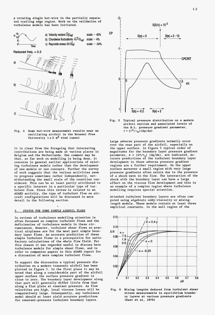
Further work at the Aerospace Department of VKI comprises the development of a one-equation model for the predfction of the transition from laminar to turbulent flow (Deyle 6 Grundmann. 1990). Simi- lar work. using modifications of a two-equation turbulence model. is going on at Ghent University. Figure 3 shorts the turbulence intensity development in the transition region of a boundary layer as measured and computed with a two-equation wdel and taking into account the turbulent flow int-mittency (Vancouilli 6 Dick, 1988).

I!

I(

!

( 10 20 Y ("1

Fig. 3 Turbulence intenmity in a boundary layer transition zwgion. Comparison between ewe.- riment m d calculstions at Ghent lkiveraitg based on L turbulence =del with sa allo- .nuCB for intermittency

At the Ewiromntal and Applied Fluid Dp.nicm Department of VKI non-linear algebraic Reynolds stress models have been tested with encouraging results for tha prsdiftion of the turbulent flow over a back-ward facing step (bnocci 6 Skov-d. 1989). An other direction of research conce- droplet transport in turbulent flows using different turbulence models. Further. large-eddy sipu- lations of turbulent flows are being carried out. first in a 2D c h a m 1 (Pinelli 6 Bennoci, 1989),

layers are under development. Numerical airmlations of the large edd1.a in turbulent flan is also e research topic of Lawain I h i ~ ~ ~ ~ i t y . Finally, at the Free University of Bmsels extnuive maawe- menta have been carried out in the shear layers of an oscillating LUCII 0012 airfoil (Da Ruyk et 11, 1988). Figure 4 shows typical results obtained with

While extensions to 30 ChnmelS and frsa-shear

a rotating single hot-wire in the partially separated trailing adge region. Work on the validation of turbulence models has been initiated.

a) v w v e d o m - i j srAe:-40?$ b) Cbhb-mAId &-4% " P L 0 Th* E) Flqmlds "9 "2d & - 44%

-2 r

0(6/C).10~

~eduoad freq. - 0.3

Fig. 4 Some hot-wire mewurement results near .D oBcillating airfoil in the Bmsmel Free UniverBitg 1 x 2 mz wind tunnel

It is clear from the foregoing that interesting contributions are being made at various places in Belgium and the Netherlands. One comment may be that, so far vork on modelling is being done, it concerns in general earlier applications of sxist- ing turbulence models rather than the development of nev models or nev concepts. Further the survey of vork suggests that the various activities Beem to progress sometimes rather independently, not- withstanding the small scale of the countries considered. This can be at least partly attributed to a specific interest in a particular type of turbulent flov. Since this reviev is related to an AGARD activity, the type of turbulent flov on aircraft configurations will be discussed in more detail in the folloving section.

In revievs of turbulence modelling attention is often focusBed on complex turbulent flors and the defieienciae of turbulence models in these cir- c-tmcea. Hovever, turbulent shear flovs on practical airplanes are far the most part slmple boundary layer flow. An accurate prediction of these simple turbulent flovs is e prerequisite for satin- factory calculations of the wholn flow field. For this reason it vas regarded useful to discuss here turhulence models for simple shear flovs, and to refer to companion papers in this AGARD report for a discussion of more complex turbulent flovs.

To support the discussion a typical pressure distribution on a modern transonic airfoil has been plotted in figure 5. In the first place it may be noted that along a considerable part of the airfoil upper surface the surface pressure gradient is close to zero. The boundary layer development along that part vi11 generally differ little from that along a flat plate at Constant preaaure. As f lov velocities are high, local visc- losees vi11 be comparatively large. Consequently, any turbulence model should at least yield accurate predictions for constant-pressure turhulsnt boundary layers.

I

Fig. 5 Typical pressure distribution on a mdern airfoil section mud associated levels of the B.L. pressure gradient parameter, n = (6*/T,) (dP/dx)

Large adverse pressure gradients normally occur over the rear part of the airfoil, especially on the upper Burface. In figure 5 typical order of magnitudes for the boundary layer pressure gradient parameter, s - (6*/r,) (dp/dx), are indicated. AC- curate predictions of the turbulent boundary layer development in these adverse pressure gradient regions are a further requirement. On the upper surface moreover a small region with very large pressure gradients often exists due to the prcaence of a shock vave in the flov. The lntsraction of the shock vith the boundary layer can have a large effect on the viscous flov development and this in an example of a complex region vhere turbulence modelling requires special attention.

Attached turbulent boundary layers are often computed using algebraio eddy-viscosity or mixing- length models. These models contain at least three empirical constants. In the vall region of the

0.12

0.10 116

0.08

0.08

0.04

0.M

0 0.1 02 03 0.4 0.5 0.8 0.1 OB ~16

Fig. 6 Mixing length. deduced fro8 turbulent shear strsms measuremntm in equilibrium bouuda- rg 1syers at various pressure gradients Want at 81, 1979)

1-4

boundary layer outside the viscous sublayer the turbulent shear stress. 7 , is normally expressed in the mixing length relation r - lzp(8U/By)z with 1 - k.y. In this relation is y the distance to the wall and k one of the empirical constants, the 80-

called Von K a m n constant. Evidence is gradually accumulating. however. that the value of k is not a constant, but depends on the surface pressure gradient. nixing length variations. deduced from tur- bulsnee measurement8 in equilibrium boundary layers at different non-dimensionalired presmre gradients r, have been plotted in figure 6 (East et al, 1979). According to these measurements the value of k varies widely and differs generally substantially from the usually assumed value for the constant. k - 0.4 .

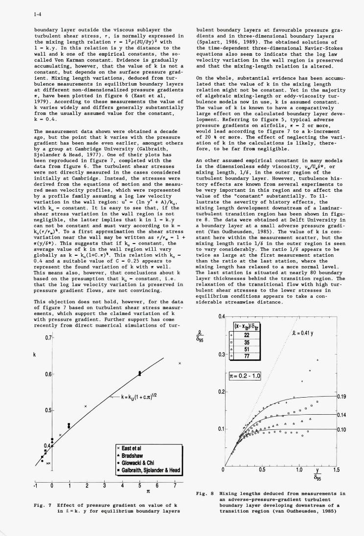
The measurement data shown were obtained a decade ago, but the point that k varies with the pressure gradient has been made even earlisr, amongst others by a group at Cambridge University (Galbraith. Sjolandsr 6 Head, 1977). One of their plots has been reproduced in figura 7. completed with the data from figure 6. The turbulent ehear stresaes were not directly measured in thhe cases considered initially at Cambridge. Instead, the stresses were derived from the equations of motion and the measured mean velocity profiles, which -re represented by a profile family assuming a log law velocity variation in the wall region: U* - (In y' + A ) A , with k,, - constant. It is easy to see that, if the shear stress variation in thhe wall region is not negligible, the latter implies that k in 1 - k.y can not be conetant and m B t vary according to k - k(r/r-)'. To a first approximation the shear stress variation near the wall may be witten as */vw - 1 + r(y/6*). This suggests that if k,, - constant, the average value of k in the wall region will vary globally as k - k,,(l+C.r)'. This relation with k,, - 0 . 4 and a suitable value of C - 0.25 appears to represent the found variation of k with r wall. This means also, however, that conclusions about k based on the presumption that k,, - constant, i.e. that the log law velocity variation is preserved in preesure gradient flows. are not convincing.

This objection does not hold, however. for the deta of figure 7 based on turbulent shear stress measurements. which support the claimsd variation of k with preseure gradient. Further support hae come recently from direct numerical simulations of tur-

0.71

k

k- k,(l+ c.nfR

0.5

1

I O 1 2 3 4 5 6 7 n

Pig. 7 Effect of pressure gradient on value of k in t = k . y for equilibrium bomdsry layem

bulent boundary layers at favourable pressure gradients and in three-dimensional boundary layers (Spalart. 1986. 1989). The obtained solutions of the time-dependent three-dimensional Navier-Stokes equations also seem to indicate that the log law velocity variation in thhe wall region i~ presarved and that the mixing-length relation is altered.

On the whole, substantial evidence has been accumu- lated that the value of k in the mixing length relation might not be constant. Yet in the llajority of algebraic mixing-length or eddy-viscosity turbulence models now in use, k is assumed constant. The value of k is known to have a coqaratively large effect on thhe calculated boundary layer development. Referring to figure 5, typical adverse pressure gradientB on airfoils, I - 2 or more, would lead according to figure 7 to a k-increment of 20 6 or more. The effect of neglecting the variation of k in the calculations is likely, therefore, to be far from negligible.

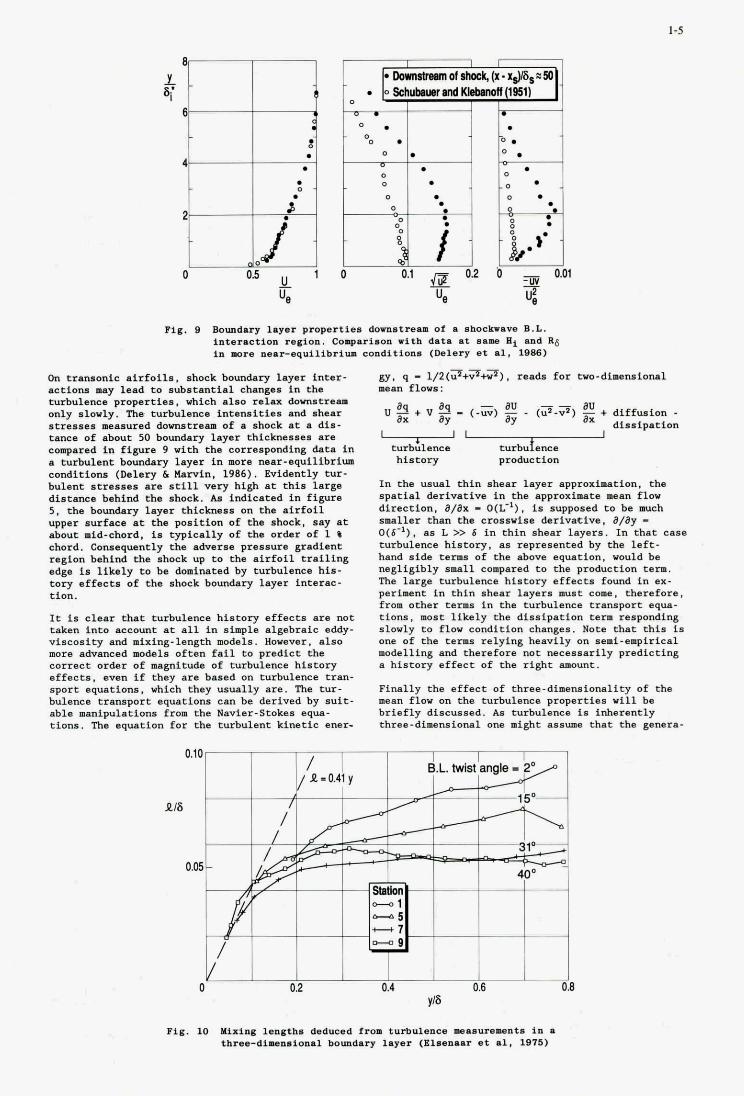
An other assunad empirical Constant in many models is the dimensionless eddy viscosity, u,/U,6*, or mixing length, 1/6, in the outer region of the turbulent boundary layer. However, turbulence history effects are known from several experimenrs to be very important in this region and to affect the value of the "constant" substantially. To illustrate the severity of history effects, the mixing length development downstream of a laninar- turbulent transition region has been shown in figure 8. The data were obtained at Delft University in a boundary layer at a small adverse pressure gradient (Van Cukeusden, 1985). The value of k is o m - stant here within the masurement scatter, but the mixing length ratio 1/6 in the outer ragion is seen to vary considerably. The ratio 1/6 appears to be twice as large at the first measurement atation than the ratio at the last station. where the mixing length has relsxd to a more normal level. The last station is dtuated at nearly 80 boundary layer thicknesses behind the transition region. The relaxation of the transitional flow with high turbulent shear stresses to the lower stresses in equilibrium conditions appears to take a con- siderabla streamwine distance.

f

0.19

0.14

0.10

5

Pig . 8 Miring lengths deduced from measurements in UI .dve=.O-preaaur~-IrPdi..t turbulent boundary layer developing domatream of a trsusition region (vsu Oudheu.den, 1886)

1-5 I

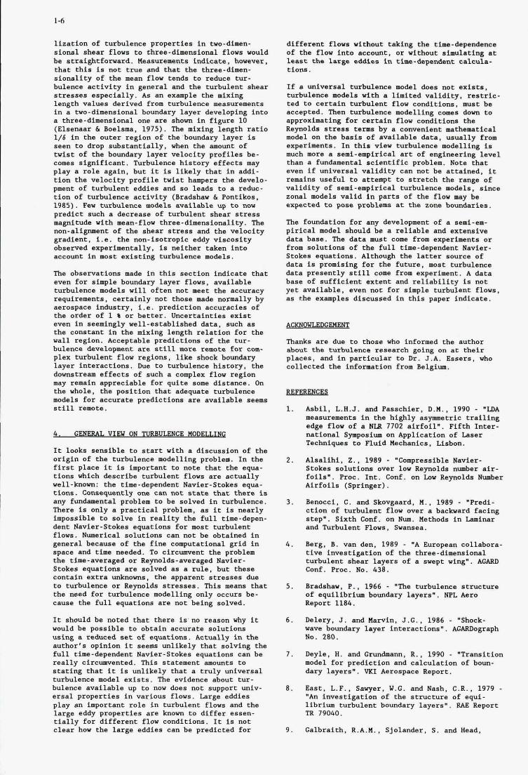
Fig,. s Boundary layer propertiem downstream of s shockwave B.L. interaftion relion. Coqarison with data at .am Et m d Rg in more nearequilibrium conditions (Delsry et a1, 1988)

00 tr-onic airfoils, shock boundary layer inter- acti- may lead to .ubstantial changes in the turbulence properties, which also r d u d0yMtre.m only slmly. The turbulence intewitias and shear stresses meaured downstream of a shock at a dis- tame of about 50 boundary layer thicknesses are compared in figure 9 with the corresponding data in a turbulent boundary layer in more near-equilibrium COnditiOM (Delery & Mrvin, 1986). Evidently turbulent stresses are still very high at this large distance behind the shock. Aa indicated in figure 5, the boundary layer thickness on the airfoil upper surface at the podtion of the shock. say at about mid-chord, is typically of the order of 1 e chord. Consequently the adverse pressure gradient region behind the lihoek up to the airfoil trailing edge is likely to be dominated by turbulence history effects of the Bhoek boundary layer interaction.

It is clear that turbulence history effects are not taken into account at all in simple algehraic eddy- viscosity and mixing-length models. Howaver, also more advanced models often fail to predict the correct order of llagnitude of turhulence history effects. even if they are based on turbulence tran- Bport equations, which they usually are. The turbulence transport equations can be derived by suft- able manipulations from the Navisr-Stoke8 equati-. The equation for the turbulent kinetic ener-

0.1

PIS

OS

W. P - 1/2(?WT+iT), reads for two-dimaneiolul mean flows:

I

tur b h 1 a nc e turbuf enca himtory production

I

In the usual thin shear layer approximation. the spatial derivative in the approximate mean f lov direction, B/Bx - O(L-l), is aupposed to be much smaller than the crosswise derivative, alar - O ( 6 - l ) . as L >> 6 in thin shear laysrll. In that case turbulance history, 88 represented by the left- hand side terms of the ahova equation, would be negligibly small compared to the production term. The large turbulence hiatory effects found in experiment in thin ahear layers muat come, therefore, from other terms in the turbulence transport equations. nost likely the dissipation term responding slowly to flow condition changes. Note that this is one of the term relying heavily on aeni-empirical modelling and therefore not necessarily predicting a history effect of the right amount.

Finally the effect of three-dimansi-lity of the mean flow on the turhulenca properties will be briefly discussed. Aa turbulence in inherently thres-dinsndmal one night a~sume that the genera-

0.2 0.4 0.6

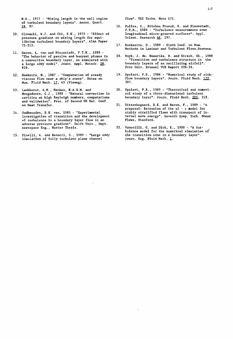
Fig . 10 IUSing, lengths deduced from turbulence IsaSUreWntS in three-dimensional boundary lager (Il1sen.u et al, 1915)

liration of turbulence properties in two-dimensional shear flows to three-dimensional flows would be straightforward. Neasurements indicate, however, that thilr is not true and that the three-dimensionality of the mean flow tends to reduce turbulence activity in general and the turbulent shear stresses especially. As an example the mixing length values derived from turbulence measurements in a two-dimensional boundary layer developing into a three-dimensional one are shown in figure 10 (Elsenaar 6 Boelsma, 1975). The mixing length ratio 1/6 in the outer region of the'houndary layer is seen to drop substantially, when the amount of twist of the boundary layer velocity profiles becomes significant. Turbulence history effects may play a role again, but it is likely that in addition the velocity profile twist hampers the development of turbulent eddies end so leads to a reduction of turbulence activity (Bradshaw 6 Pontikos. 1985). Few turbulence models available up to now predict such a decraastr of turbulent shear stress magnitude with mean-flow three-dimensionality. The non-alignment of the shear stress and the velocity gradient, i.e. the non-isotropic eddy viscosity observed experimentally, is neither taken into account in most existing turbulence models.

The observations made in this section indicate that even for simple boundary layer flows. available turbulence models will often not meet the accuracy requirements. certainly not those made normally by aerospace industry. i.e. prediction accuracies of the order of 1 % or batter. Uncertainties exist even in seemingly well-established data, such as the constant in the mixing length relation for the wall region. Acceptable predictions of the tu=- bulence development are still more remote for con- plex turbulent flow regions, like shock boundary layer interactions. Due to turbulence hiscory. the downstream effects of such a complex flow region may remain appreciable for quite some distance. On the whole, the position that adequate turbulence models for accurate predictions are available seems still remote.

4. G E N E U L VIEW ON TIIBBULENCE N O W

It looks sensible to start with a discussion of the origin of the turbulence modelling problem. In the first place it is important to note chat the aqua- tions which describe turbulent flows are actually well-known: the time-dependent Navier-Stokes equations. Consequently one can not state that there is any fundamental problem to he solved in turbulence. There is only a practical problem, as it is nearly impossible to solve in reality the full time-dependent Navier-Stokes equations for most turbulent flows. Numerical solutions can not be obtained in general because of the fine. computational grid in space and time needed. To circumvent the problem the time-averaged or Reynolds-averaged Navier- Stokes equations are solved as a rule, but these contain extra unlmovns, the apparent stresses due to turbulence or Reynolds stresses. This means that the need for turbulence modelling only occurs because the full equations are not being solved.

It should be noted that there is'no reason why it would be possible to obtain accurate solutions using a reduced set of equations. Actually in the author's opinion it seems unlikely that solving the full time-dependant Navier-Stokes equations can he really circumvented. This statement amounts to stating that it is unlikely that a truly universal turbulence model exists. The evidence about tu=- bulence available up to now does not support universal properties in various flows. Large eddies play an important role in turbulent flows end the large eddy properties are known to differ essentially for different flow conditions. It is not clear how the large eddies can be predicted for

different flows without taking the time-dependence of the flow into account, or without simulating at least the large eddies in time-dependent calculations.

If e universal turbulence model does not exist.. turbulence models with a limited validity. rsstric- red to certain turbulent flow conditions, must be accepted. Then turbulence modelling comes down to approximating for cercain flow conditions the Reynolds stress term by a convenient mathematical model on the basis of available data, usually from experiments. In this view turbulence modelling is much mors a semi-empirical art of engineering level then a fundamental scientific problem. Note thac even if universal validity can not be attained, it remains useful to attempt to stretch the range of validity of semi-empirical turbulence models, since zonal models valid In parts of the flow may be expected to pose problems at the zone boundaries.

The foundation for any development of a aemi-empirical model should be a reliable and extensive data base. The data must come from experiments or from SOlUtiOM of the full time-dependent Navisr- Stokes equations. Although the latter source of data is promising for the future. most turbulence data presently still come from experiment. A data base of sufficient extent and reliability is not yet available, even not for simple turbulent flows, as the examples discussed in this paper indicate.

Thanks are due to those who informed the author about the turbulence research going on at their places, and in particular to Dr. J.A. Essers. who collected the information from Belgium.

REFeRENCES

1.

2.

3 .

4.

5 .

6.

7.

8.

9.

Asbil, L.H.J. and Passchier, D.H., 1990 ~ "LDA measurements in the highly asymmetric trailing edge flow of a N U 7702 airfoil". Fifth Inter- national Symposium on Application of laser Techniques to Fluid Kechanics, Lisbon.

Alsalihi. 2. . 1989 - "Compressible Navier- Stokes solutions over low Reynolds number airfoils". Proc. lnt. Conf. on Low Reynolds Number Airfoils (Springer).

Benoeci, C. and Skovgaard. U,. 1989 - "Predi- ction of turbulent flow over a backward facing step". Sixth Conf. on Nu. Nethoda in Laminar and Turbulent Flows, Swansea.

Berg, 8 . van den, 1989 - "A European collebora- tive investigation of the three-dimensional turbulent shear layers of a swept wing". AGARD Conf. Proc. No. 438.

Bradshaw, P., 1966 - "The turbulence structure of equilibrium boundary layers". NPL Aero Report 1184.

Delery, J. and hrvin. J . G . , 1986 - "Shock- wave boundary layer ineeractions". AGARDograph No. 280.

Deyle. H. and Gmdmann, R., 1990 - "Transition model fOK prediction and calculation of boundary layers". VKI Aerospace Report.

East, L . F . , Sawyer, W.G. and Nash, C.R., 1979 "An investigation of the structure of equilibrium turbulent boundary layers". QAE Report TR 79040.

Galbraith. R.A.K., Sjolander. S. and Haad,

1-7

1 10.

11. 1

12.

13.

14.

15.

M.R., 1977 - "Mixing length in the wall region of turbulent boundary layers". Aeron. Quart. - 28. 97.

Glowacki, W.J. and Chi, S.W., 1972 - "Effect of pressure gradient on mixing length for equilibrium turbulent boundary layers". AIAA Paper 72-213.

Haren, L. van and Nieuwstadt, F.T.M., 1989 - "The behavior of passive and buoyant plumes in a convective boundary layer, as simulated with a large eddy model". Journ. Appl. Meteor. 28, 818.

Hoekstra, M., 1987 - "Computation of steady viscous flow near a ship's stern". Notes on Num. Fluid Mech. U , 45 (Vieweg).

Lankhorst, A.M., Henkes, R.A.W.M. and Hoogedoorn, C.J., 1988 - "Natural convection in cavities at high Rayleigh numbers, computations and validation". Proc. of Second UK Nat. Conf. on Heat Transfer.

Oudheusden, B.W. van, 1985 - "Experimental investigation of transition and the development of turbulence in a boundary layer flow in an adverse pressure gradient". Delft Univ., Dept. Aerospace Eng., Master Thesis.

Pinelli, A. and Benocci, C., 1989 - "Large eddy simulation of fully turbulent plane channel

flow". VKI Techn. Note 171.

16. Pulles, C., Krishna Prasad, K. and Nieuwstadt, F.T.M., 1989 - "Turbulence measurements over longitudinal micro-grooved surfaces". Appl. Scient. Research 46, 197.

17. Roekaerts, D., 1989 - Sixth Conf. on Num. Methods in Laminar and Turbulent Flows,Swansea.

18. Ruyk, J. de, Hazarika, B. and Hirsch, Ch., 1988 - "Transition and turbulence structure in the boundary layers of an oscillating airfoil". Free Univ. Brussel W B Report STR-16.

19. Spalart, P.R., 1986 - "Numerical study of sink- flow boundary layers". Journ. Fluid Mech. U , 307.

20. Spalart, P.R., 1989 - "Theoretical and numerical study of a three-dimensional turbulent boundary layer". Journ. Fluid Mech. 205. 319.

21. Uittenbogaard, R.E. and Baron, F., 1989 - "A proposal: Extension of the q2 - c model for stably stratified flows with transport of internal wave energy". Seventh Symp. Turb. Shear Flows, Stanford.

22. Vancoilli, G. and Dick, E., 1988 - "A turbulence model for the numerical simulation o i the transition zone in a boundary layer". Journ. Eng. Fluid Mech. 1.

2- 1

SUMMARY

TION OF T U R B U L E N T L O W S

J. COUSTEIX ONERA/CERT

Complexe scientifique de Rangueil 2 avenue E. Belin

31055 Toulouse CCdex FRANCE

This paper discusses the use and the suitability of turbulence models for calculating compressible flows in Aerodynamics. As the compressible form of turbulence models is generally extended from a basic incompressible form, the emphasis is placed on the pertinence of these extensions and on the peculiarities of compressible flows.

The calculation of compressible turbulent flows in Aerodynamics has been performed by using more or less empirical methods. These methods include correlations techniques and integral methods for calculating boundary layer flows. Such methods are still in use today but is is clear that more detailed or more accurate methods are needed.

In the seventies a great hope has been placed in the development of transport equation models to represent the effects of turbulence on the mean flow. After a period of enthusiasm where these techniques enabled us to make a decisive step towards a real improvement in the calculation methods of turbulent flows, it appears that the progress is now much slower.

This paper is trying to state where we are with the turbulence models, what is being done and what could or should be done to improve these turbulence models.

OF TURBULENT - 2.1.1 De.€W.wn of aver- . .

For practical applications, the calculation of turbulent flows is approached by using statistical equations which are :

(1 ) i+W + - 0

a t axi

where < > denotes a statistical average.

The main question is to choose how to decom- pose and in equations (1) and (2). The decomposition of <fij> is less important because the viscous stresses are negligible in turbulent flow. A discussion of this problem has been done by CHASSAING. 1985.

The pressure and the density are decomposed as : p = + p' ; = 0 p = + p ' ; = O but many possibilities can be used to decom- pose the velocity.

If we use the decomposition : ui = < ui > + U') ; < U"i > = 0 we have : = < ~ i > + < p' ~ " i > = < Ui > < ~j > + < P' ~ " i > < ~j >

+ < p' U') > < Ui > + < ,"i > < U'\ > + < P' ,"i ,"j >

Compared with the incompressible case, many additional terms appear and the formulation of equations is very complicated.

Most of the works use a mass-weighted velocity ui. This type of average has been introduced by FAVRE, 1958, in turbulence studies. We have :

-

The average equations are :

(4)

2-2

Equations (4) and (5 ) have an "usual" form in the sense that they look like their incompressible counterpart.

The concept of average stream surface has the same meaning as in incompressible flow. In addition, the equations for the Reynolds stresses - < p' u'i u'j > are obtained in a natural way and not too many additional terms are in- t roduced. The danger is that the equations are too close to the incompressible case and it is tempting to apply them an "incompressible" closure,which is not always justified. It is worth mentioning that many other decomposition are possible and this problem is not closed. Nevertheless the mass-weighted averages are used in the rest of this paper.

2.1 .2 . Eauations with mass-weighted aye rapes

To simplify the writing of the averaged equations, is written p. For example, we have :

but when p is combined with a random function inside a sign <>, the same convention does not apply :

When no confusion is expected, the sign (-) is omitted :

- pUi = U i

<pu'iU'j> # <U'iu'j>

h = h

Continuity equatio n

*+aPUk - 0 a t axk

Momentum eau ation

with

At high REYNOLDS number, the viscous stress Fik is negligible compared with the turbulent stress - p < u'i u'k >. Near a wall, this is no longer true. Even if the fluctuations of viscosity are neglected, the expression of Fjk is not simple because :

Kinetic enerev eauat ions

The mean value of kinetic energy is decomposed as :

The first part K corresponds to the averaged motion and the second part k to the fluctuations.

The corresponding equations are :

w i t h

The dissipation rate of the instantaneous kine- aui

tic energy is cp = fik - Its averaged value is

decomposed as :

w i t h

a X k '

 is the dissipation rate of the averaged kinetic energy of the fluctuating motion which appears in eq. 9b. The exchange of energy between K and k is represented by the work of

aUi the REYNOLDS stresses - <pU'jU'k>-. axk

In the k-equation, the compressibility appears

explicity. through two terms : <p' -> a n d au'j

axi

2-3

<p'u'i> aP P axi

. This does not mean however that --

the compressibility cannot influence other terms.

R- S i n

We define Tij as :

The REYNOLDS stress equation is :

DT. a P = P Pij.- P Dij +P @ij + P Cij + -,(P Jijk) (1 0)

axk Dt

The interpretation of this equation is nearly the same as in incompressible flow. PPjj is the production term ; ~ D i j is the destruction term

(p is the dissipation of k) ; P @ij is the

velocity-pressure correlation ; PJijk is the diffusion due to interactions between velocity fluctuations, due to viscosity and due to interactions between pressure and velocity.

DA

The compressibility appears explicitly only through the term Cij but, once again, the modelled form of the other terms can be influenced by compressibility. For example, the modelling of Oij is based on the POISSON equation for p' which is obtained by taking the divergence of the momentum equation. In this equation, many additional terms appear due to the compressibility of the flow :

The flows under consideration are characterized by a high Mach number and very often by a heat transfer at walls. Therefore heat is produced by direct. dissipation and transferred by the turbulent fluctuations.

These phenomena imply a non uniform averaged temperature .and density, which influence the velocity field.

In a boundary layer developing on an adiabatic wall, the large amount of dissipation near the wall leads to a large static temperature in this region. Then the kinematic viscosity is larger than near the external edge of the boundary layer and the local REYNOLDS number is smaller. Compared with an incompressible boundary layer, the viscous sublayer is thicker.

The variation of density in itself does not imply a modification of the turbulence structure. For example, the study by BROWN and ROSHKO of a low-speed mixing layer with a mixing of gases with different densities showed that the spreading rate of the layer is not affected by the variation of density. On the contrary, the spreading rate of a mixing layer of air is significantly reduced in supersonic flow. This means that there is a genuine compressibility effect in this case. It is not clear however if this is due to an effect on the turbulence structure. At least partly, the reduction of the spreading rate can be attributed to an effect of compressibility on the stability properties of the flow which are at the origin of the large scale structures. PAPAMOSCHOU-ROSHKO studied ten configurations of free shear layers obtained by using the flow of various gases (N2, Ar, He) at various MACH numbers (between 0.2 and 4). These authors introduced a convective MACH number which is .defined in a coordinate system moving with the convection velocity of the dominant waves and structures of the shear layers. The , theoretical analysis is performed by studying the stability of a compressible inviscid vortex sheet. PAPAMOSCHOU-ROSHKO showed that the growth rates of the various free shear layers fall nearly onto a single curve. This result indicates that the shear layer question is more related to a stability problem than to a turbulence problem.

Another feature of compressible flows is that all the flow characteristics are fluctuating : velocity, temperature, density and pressure.

KOVASZNAY showed that these fluctuations can be expressed as a function of three basic modes

2-4

(see .FAVRE et al.) : fluctuations of vorticity, entropy and pressure (acoustic fluctuations) and when the level of fluctuations is low, the equations describing the evolution of vorticity and pressure are separated. (The correlation coefficients between the various modes are not necessarily low).

When the fluctuations are no longer low, a second order theory predicts various possible interactions between modes. In supersonic flows, a strong interaction is the vorticity-vorticity interaction which is at the origin of the aerodynamic noise.

These flows are also characterized by the pressure fluctuations (which are isentropic) which can be transmitted over long distances as MACH waves. The loss of turbulent energy by sound radiation is low but the radiated energy can have a strong effect on the laminar-turbulent transition. In supersonic and hypersonic wind tunnels, the transition on a flat plate or on a cone is strongly dependent on the noise generated by the turbulent boundary layers developing on the test section walls. The transition location is correlated with the test section size because the noise affecting the transition depends on the distance between the model and the tunnel walls.

The role played by the pressure fluctuations in the turbulence modelling can be very different in compressible or incompressible flows. For example, the influence of compressibility on

au'i the <P' -> term appears through the axi

POISSON equation for the pressure which contains much more terms in a compressible flow.

The averaged pressure gradient can also modify the processes of turbulence generation or destruction in supersonic flows. The pressure gradient can be very strong (through a shock wave or an expansion fan) and the interaction with the term <p"i> in the turbulent kinetic

energy equation can be significant. This also means that the wall curvature is an important parameter because it implies the existence of a normal pressure gradient and an effect on the turbulence.

P

Let us go back to the decomposition of the turbulent field into three modes : vorticity, entropy and acoustic pressure. At low MACH numbers in an isothermal flow, only the vorticity mode remains. In a compressible flow, if the vorticity generation by interactions between modes is negligible, the turbulence structure is unaffected by compressibility (the

possible vorticity generation interactions are vorticity-entropy, vorticity-acoustic pressure, entropy-acoustic pressure).

From experimental data, MORKOVIN, 1961, showed that the acoustic mode and the entropy mode are negligible in boundary layers with usual rates of heat transfer and Me < 5.

According to MORKOVIN, these flows are such as :

c<< P 1 ; g < < 1

Using the state law and assuming that the velocity fluctuations u'/U are not too large, we have :

The following relationships are deduced :

This is the so-called strong REYNOLDS analogy. In fact, the basic hypotheses presented above are not very well founded and improvements of the analysis have been proposed by GAVIGLIO, 1987. Nevertheless, practical results such as formulae (12) can give reasonable orders of magnitude. For example, in a boundary layer on an adiabatic wall in supersonic flow, ruiT* is of order - 0.8.

The use of the strong REYNOLDS analogy should be done with care, in particular when the flow undergoes rapid variations.

It should also be noticed that some of the formulae deduced from the strong REYNOLDS analogy are not galilean invariant ; this is the case of the formula (12a) because M*/U is not galilean INVARIANT.

BRADSHAW, 1977, associated the validity of the MORKOVIN hypothesis with low values of .-

<p'2>'D . For boundary layers with an external P

MACH number lower than 5. the condition is

fulfilled as - is smaller than 0.1.

BRADSHAW noticed that at higher MACH numbers, the total temperature fluctuations are no longer negligible but when the wall is cooled, the level of temperature and density fluctuations increases only slowly with the MACH number. At these higher MACH numbers, the pressure fluctuations increase and the turbu-

< p'2> 112

P

2-5

lence structure can be affected (pressure-vorticity and pressure-entropy interactions can generate vorticity fluctuations).

BRADSHAW also noticed that in free mixing layers, the level of velocity fluctuations <u12>1/2/U can reach 0.3 so that the density fluctuations are larger. This implies that the limit of validity of the MORKOVIN hypothesis ( < ~ ' ~ > ' / ~ / p < 0.1) is limited to external MACH number less than 1.5. This is in rough agreement with experimental data but as already said, it is not clear if the effect of Mach number on the spreading rate of the mixing layer is due to an alteration of the turbulence structure or to an effect on the stability of the flow (which is at the origin of the large structures).

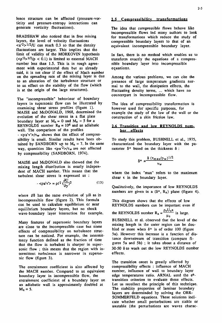
The "incompressible" behaviour of boundary layers in supersonic flow can be illustrated by examining shear stress profiles (figure 1). MAISE and McDONALD. 1968, determined the evolution of the shear stress in a flat plate boundary layer at Me = 0 and Me = 5 for a REYNOLDS number Re = 104 and an adiabatic wall. The comparison of the profiles - <pu'v'>/.rw shows that the effect of compressibility is small. Similar results have been obtained by SANDBORN up to Me = 7. In the same way, quantities like <pu'2>/.rw are not affected by compressibility (SANDBORN, 1974).

MAISE and McDONALD also showed that the mixing length distribution is nearly independent of MACH number. This means that the turbulent shear stress is expressed as :

a u ay

- <pu'v'> = pc2 (-)2

where U6 has the same evolution of y/6 as in incompressible flow (figure 2). This formula can be used to calculate equilibrium or near equilibrium boundary layers, but no shock wave-boundary layer interaction for example.

Many features of supersonic boundary layers are close to the incompressible case but some effects of compressibility on turbulence structure can be noticed. For example, the intermittency function defined as the fraction of time that the flow is turbulent is sharper in supersonic flow ; this means that the region with intermittent turbulence is narrower in supersonic flow (figure 3).

The entrainment coefficient is also affected by the MACH number. Compared to an equivalent boundary layer in incompressible flow, the entrainment coefficient of a boundary layer on an adiabatic wall is approximately doubled at Me = 5.

C-v transformations . . . The idea that compressible flows behave like incompressible flows led many authors to look for transformations which reduce the study of compressible boundary layers to that of an equivalent incompressible boundary layer.

In fact, there is no method which enables us to transform exactly the equations of a compressible boundary layer into incompressible equations.

Among the various problems, we can cite the presence of large temperature gradients normal to the wall, the dissipation effects, the fluctuating density terms, ... which have no counterpart in incompressible flow.

The idea of compressibility transformation is however used for' specific purposes, for example the study of the law of the wall or the construction of a skin friction law.

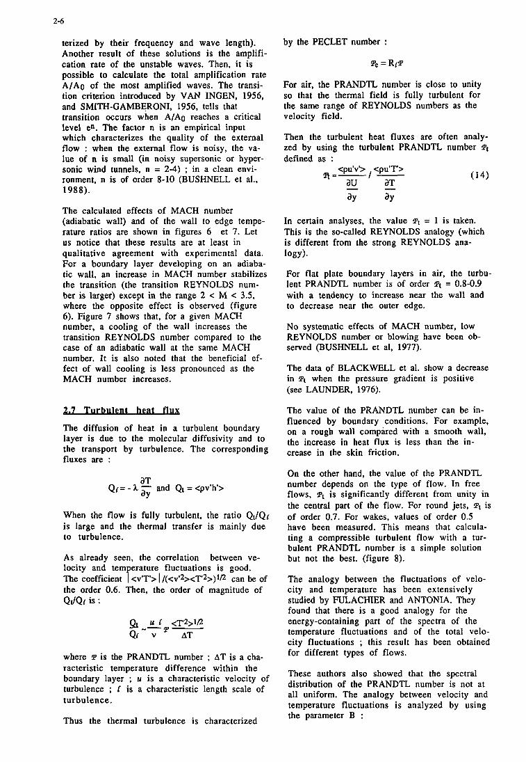
To study this problem, BUSHNELL et al., 1975, characterized the boundary layer with the parameter 6+ based on the thickness 6 :

where the index "max" refers to the maximum shear z in the boundary layer.

Qualitatively, the importance of low REYNOLDS numbers are given in a (6+, R,) plane (figure 4).

This diagram shows that the effects of low REYNOLDS numbers can be important even if

is large. PeUex the REYNOLDS number R, =- Pe

BUSHNELL et al. observed that the level of the mixing length in the outer region can be doubled or more when 6+ is of order 100 (figure 5a). However this increase is a function of distance downstream of transition (compare figures 5a and 5b) ; it takes about a distance of 30-50 6 to wash out the low REYNOLDS number effects.

The transition onset is greatly affected by compressibility effects : influence of MACH number, influence of wall to boundary layer edge temperatures ratio. ARNAL used the en- transition criterion to evaluate these effects. Let us recollect the principle of this technique. The stability properties of laminar boundary layers are determinded by solving the ORR- SOMMERFELD equations. These solutions indicate whether small perturbations are stable or unstable (the perturbations are waves charac-

2-6

terized by their frequency and wave length). Another result of these solutions is the amplification rate of the unstable waves. Then, it is possible to calculate the total amplification rate A/Ao of the most amplified waves. The transition criterion introduced by VAN INGEN, 1956, and SMITH-GAMBERONI, 1956, tells that transition occurs when A/Ao reaches a critical level en. The factor n is an empirical input which characterizes the quality of the external flow : when the external flow is noisy, the value of n is small (in noisy supersonic or hypersonic wind tunnels, n = 2-4) ; in a clean envi- ronment, n is of order 8-10 (BUSHNELL et al., 1988).

The calculated effects of MACH number (adiabatic wall) and of the wall to edge temperature ratios are shown in figures 6 us notice that these results are at least in qualitative agreement with experimental data. For a boundary layer developing on an adiabatic wall, an increase in MACH number stabilizes the transition (the transition REYNOLDS number is larger) except in the range 2 < M < 3.5, where the opposite effect is observed (figure 6). Figure 7 shows that, for a given MACH number, a cooling of the wall increases the transition REYNOLDS number compared to the case of an adiabatic wall at the same MACH number. It is also noted that the beneficial effect of wall cooling is less pronounced as the MACH number increases.

et 7. Let

2.7 Turbulent heat flux

The diffusion of heat in a turbulent boundary layer is due to the molecular diffusivity and to the transport by turbulence. The corresponding fluxes are :

When the flow is fully turbulent, the ratio QtlQr is large and the thermal transfer is mainly due to turbulence.

As already seen, the correlation locity and tem erature fluctuations is good. The coefficient P <v'T> I /(<V%<T*>)~D can be of the order 0.6. Then, the order of magnitude of

between ve-

QJQr is :

where P is the PRANDTL number ; AT is a characteristic temperature difference within the boundary layer : U is a characteristic velocity of turbulence ; C is a characteristic length scale of turbulence.

Thus the thermal turbulence is characterized

by the PECLET number :

!Pe = R(T

For air, the PRANDTL number is close to unity so that the thermal field is fully turbulent for the same range of REYNOLDS numbers as the velocity field.

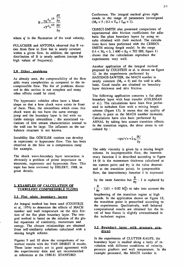
Then the turbulent heat fluxes are often analyzed by using the turbulent PRANDTL number Pt

defined as : <pu'v'> <pu'T'> a=-/- au

ay ay

aT - -

In certain analyses, the value Pt = 1 is taken. This is the so-called REYNOLDS analogy (which is different from the strong REYNOLDS analogy).

For flat plate boundary layers in air, the turbulent PRANDTL number is of order Tt = 0.8-0.9 with a tendency to increase near the wall and to decrease near the outer edge.

No systematic effects of MACH number, low REYNOLDS number or blowing have been observed (BUSHNELL et al. 1977).

The data of BLACKWELL et al. show a decrease in Pt when the pressure gradient is positive (see LAUNDER, 1976).

The value of the PRANDTL number can be influenced by boundary conditions. For example, on a rough wall compared with a smooth wall, the increase in heat flux is less than the increase in the skin friction.

On the other hand, the value of the PRANDTL number depends on the type of flow. In free flows, Pt is significantly different from unity in the central part of the flow. For round jets, Pt is of order 0.7. For wakes, values of order 0.5 have been measured. This means that calculating a compressible turbulent flow with a turbulent PRANDTL number is a simple solution but not the best. (figure 8).

The analogy between the fluctuations of velocity and temperature has been extensively studied by FULACHIER and ANTONIA. They found that there is a good analogy for the energy-containing part of the spectra of the temperature fluctuations and of the total velocity fluctuations ; this result has been obtained for different types of flows.

These authors also showed that the spectral distribution of the PRANDTL number is not at all uniform. The analogy between velocity and temperature fluctuations is analyzed by using the parameter B :

2-7

<q'31D ay Bp- -

where q' is the fluctuation of the total velocity.

FULACHIER and ANTONIA observed that B varies from flow to flow but is nearly constant within a given flow. In addition, the spectral distribution of B is nearly uniform (except for high values of frequency).

As already seen, the compressibility of the flow adds many complexities as compared to the incompressible flow. The list of problems discussed in this section is not complete and many other effects could be cited.

The hypersonic vehicles often have a blunt shape so that a bow shock wave exists in front of them. Then, the streamlines which cross this shock wave do not have the same entropy jump and the boundary layer is fed with variable entropy streamlines ; the associated variations of free stream characteristics normal to the wall can be large. The influence on the turbulence structure is not known.

Instability like GORTLER vortices can develop in supersonic or hypersonic flow. This has been observed in the flow on a compression ramp for example.

The shock wave-boundary layer interaction is obviously a problem of prime importance in transonic, supersonic and hypersonic flow. This topic has been reviewed by DELERY, 1988, in great details.

TURBULENT COMPRESS IBLE FLOWS

3.1 F lat d a t e boundarv lave rS

An integral method has been used (COUSTEIX et al. 1974) to determine the effects of MACH number and wall temperature on the skin friction of the flat plate boundary layer. The integral method is based on the solution of the global equations of continuity, momentum and energy. The closure relationships are obtained from self-similarity solutions calculated with a mixing length scheme.

Figures 9 and 10 show the comparisons of numerical results with the VAN DRIEST I1 results. These latter results are in good agreement with the experimental data and are recommended as references at the 1980-81 STANFORD

Conference. The integral method gives right trends in the range of parameters investigated (Me < 5 ; 0.2 < Tw / Tad < 1).

CEBECI-SMITH also presented comparisons of experimental skin friction coefficients for adiabatic flat plate boundary layers by using results obtained with their method. The calculations have been performed with the CEBECI- . SMITH mixing length model. In the range 0.4 < Me < 5, 1 600 < Re < 702 000, figure 11

. shows that the calculations reproduce the experiments very well.

Another application of the integral method proposed by COUSTEIX et al. is shown on figure 12. In the experiments performed by HASTINGS-SAWYER, the MACH number is nearly constant (Me = 4) and the wall is adiabatic. Good results are obtained on boundary layer thickness and skin friction.

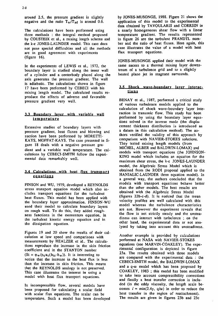
The following application concerns a flat plate boundary layer with heat transfer (COLEMAN et al.). The calculations have been first performed in turbulent flow with a mixing length scheme (figure 13). It seems that the quality of results is poor as the MACH number increases. Calculations have also been performed by ARNAL by taking into acount transition effects. In the transition region, the shear stress is calculated by :

A au -<pu'v'> = E pt - a y

The eddy viscosity is given by a mixing length scheme. In incompressible flow, the intermittency function ^E is described according to figure 14 (e is the momentum thickness calculated at the current point and 8 T is the value determined at the transition point). In compressible flow, the intermittency function ^E is expressed

by the same function but - - 1 is replaced by 0 eT

e ( - - 1)/(1 + 0.02 MZ) to take into account the eT lengthening of the transition region at high speeds. In the application shown on figure 15, the transition point is prescribed according to the experiments. Qualitatively, well behaved computational results are obtained but the level of heat fluxes is slightly overestimated in the turbulent region.

3.2 B o W r p laver with Dressure g r k dient

In the experiments of CLUTTER-KAUPS, the boundary layer is studied along a body of re- volution with different conditions of velocity, pressure gradient and wall temperature. In the example presented, the MACH number is

2-8

around 2.5, the pressure gradient is slightly negative and the ratio Tw/Tad is around 0.6.

The calculations have been performed using three methods : the integral method proposed by COUSTEIX et al., a mixing length scheme and the k-E JONES-LAUNDER model. This case does not pose special difficulties and all the methods are in good agreement with experiments (figure 16).

In the experiments of LEWIS et al., 1972, the boundary layer is studied along the inner wall of a cylinder and a centerbody placed along the axis generates the pressure gradient. The wall is adiabatic.. The calculations shown .in figure 17 have been performed by CEBECI with his mixing length model. The calculated results reproduce the effects of adverse and favorable pressure gradient very well.

Extensive studies of boundary layers with. pressure gradient, heat fluxes and blowing and suction have been performed by MORETTI- KAYS, MOFFAT-KAYS. The case presented in figure 18 deals with a negative pressure gradient and a variable wall temperature. The calculations by CEBECI-SMITH follow the experimental data remarkably well.

FINSON and WU, 1979, developed a REYNOLDS stress transport equation model which also includes transport equations for the turbulent heat fluxes. This model has been applied with the boundary layer approximation. FINSON-WU used their model to calculate boundary layers on rough wall. To do this, they added roughness functions in the momentum equation, in the turbulent kinetic energy equation and in the dissipation equation.

Figures 19 and 20 show the results of their calculation at low speed and comparisons with measurements by HEALZER et al.. The calculations reproduce the increase in the skin friction coefficient and in the STANTON number (St = qw/Peue(hie-hw)). It is interesting to notice that the increase in the heat flux is less than the increase in skin friction. This means that the REYNOLDS analogy is not preserved. This case illustrates the interest in using a model with heat flux transport equations.

In incompressible flow, several models have been proposed for calculating a scalar field with scalar flux equations. The scalar can be temperature. Such a model has been developed

by JONES-MUSONGE, 1988. Figure 21 shows the application of this model to the experimental data obtained by TAVOULARIS and CORRSIN in a nearly homogeneous shear flow with a linear temperature gradient. The results represented in figure 26 are the turbulent PRANDTL number and the ratio of heat fluxes. Here again, this case illustrates the value of a model with heat flux transport equations.

JONES-MUSONGE applied their model with the same sucess to a' thermal mixing layer downstream of a turbulence grid and to a slightly heated plane jet in stagnant surrounds.

BENAY et al., 1987, performed a critical study of various turbulence models applied to the calculation of shock wave-boundary layer interaction in transonic flow. This study has been performed by using the boundary layer equations solved in the inverse mode (the displacement thickness distribution is introduced as a datum in this calculation method). The authors verified the validity of this approach by comparison with NAVIER-STOKES solutions. They tested mixing length models (from MICHEL, ALBER and BALDWIN-LOMAX) and models with transport equations (the JOHNSON- KING model which includes an equation for the maximum shear stress, the k-e JONES-LAUNDER model, the Algebraic Stress Model which is obtained from the ROD1 proposal applied to the HANJALIC-LAUNDER three equation model). In a general way, the authors concluded that the models with transport equations behave better than the other models. The best results are obtained with the Algebraic Stress Model (figures 22b-c-d). It is noticed that the mean velocity profiles are well calculated with this model whereas the turbulence characteristics are not. However the experiment reveals that the flow is not strictly steady and the unsteadiness can interact with turbulence : on the other hand, the experimental data ar not analysed by taking into account this unsteadiness.

Another example is provided by calculations performed at NASA with NAVIER-STOKES equations (see MARVIN-COAKLEY). The experimental configuration is depicted in figure 23a. The results obtained with three models are compared with the experimental data : the CEBECI-SMITH model, the BALDWIN-LOMAX and a q-w model which has been proposed by COAKLEY, 1983 : this model has been modified to take into account compressibility corrections and finally a heat transfer correction is included (in the eddy viscosity. the length scale becomes C = min(2.4y, q/o) in order to reduce the heat transfer in the region of reattachment). The results are given in figures 23b and 23c

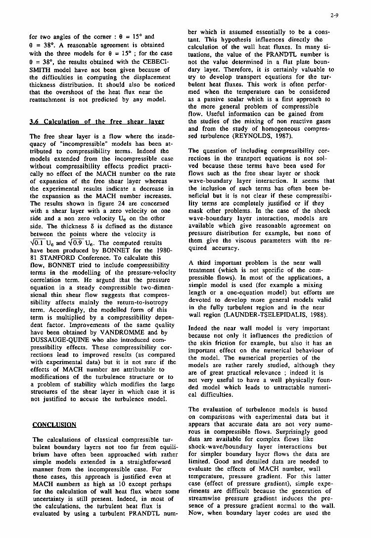
2-9

for two angles of the comer : 8 = 15' and 8 = 38O. A reasonable agreement is obtained with the three models for 8 = 15" ; for the case 8 = 38", the results obtained with the CEBECI- SMITH model have not been given because of the difficulties in computing the displacement thickness distribution. It should also be noticed that the overshoot of the heat flux near the reattachment is not predicted by any model.

3.6 C a l c w o n of the free shear lavec

The free shear layer is a flow where the inadequacy of "incompressible" models has been attributed to compressibility terms. Indeed the models extended from the incompressible case without compressibility effects predict practically no effect of the MACH number on the rate of expansion of the free shear layer whereas the experimental results indicate a decrease in the expansion as the MACH number increases. The results shown in figure 24 are concerned with a shear layer with a zero velocity on one side and a non zero velocity Ue on the other side. The thickness 6 is defined as the distance between the points where the velocity is f i v e and 40.9 Ue. The computed results have been produced by BONNET for the 1980- 81 STANFORD Conference. To calculate this flow, BONNET tried to include compressibility terms in the modelling of the pressure-velocity correlation term. He argued that the pressure equation in a steady compressible two-dimensional thin shear flow suggests that compressibility affects mainly the return-to-isotropy term. Accordingly, the modelled form of this term is multiplied by a compressibility dependent factor. Improvements of the same quality have been obtained by VANDROMME and by DUSSAUGE-QUINE who also introduced compressibility effects. These compressibility corrections lead to improved results (as compared with experimental data) but it is not sure if the effects of MACH number are attributable to modifications of the turbulence structure or to a problem of stability which modifies the large structures of the shear layer in which case it is not justified to accuse the turbulence model.

-

CO" The calculations of classical compressible turbulent boundary layers not too far from equilibrium have often been approached with rather simple models extended in a straightforward manner from the incompressible case. For these cases, this approach is justified even at MACH numbers as high as 10 except perhaps for the calculation of wall heat flux where some uncertainty is still present. Indeed, in most of the calculations, the turbulent heat flux is evaluated by using a turbulent PRANDTL num-

ber which is assumed essentially to be a constant. This hypothesis influences directly the calculation of the wall heat fluxes. In many situations, the value of the PRANDTL number is not the value determined in a flat plate boundary layer. Therefore, it is certainly valuable to try to develop transport equations for the turbulent heat fluxes. This work is often performed when the temperature can be considered as a passive scalar which is a first approach to the more general problem of compressible flow. Useful information can be gained from the studies of the mixing of non reactive gases and from the study of homogeneous compres- sed turbulence (REYNOLDS, 1987).

The question of including compressibility corrections in the transport equations is not solved because these terms have been used for flows such as the free shear layer or shock wave-boundary layer interaction. It seems that the inclusion of such terms has often been beneficial but it is not clear if these compressibility terms are completely justified or if they mask other problems. In the case of the shock wave-boundary layer interaction, models are available which give reasonable agreement on pressure distribution for example, but none of them give the viscous parameters with the required accuracy.

A third important problem is the near wall treatment (which is not specific of the compressible flows). In most of the applications, a simple model is used (for example a mixing length or a one-equation model) but efforts are devoted to develop more general models valid in the fully turbulent region and in the near wall region (LAUNDER-TSELEPIDALIS, 1988).

Indeed the near wall model is very important because not only it influences the prediction of the skin friction for example, but also it has an important effect on the numerical behaviour of the model. The numerical properties of the models are rather rarely studied, although they are of great practical relevance ; indeed it is not very useful to have a well physically founded model which leads to untractable numerical difficulties.

The evaluation of turbulence models is based on comparisons with experimental data but it appears that accurate data are not very numerous in compressible flows. Surprisingly good data are available for complex flows like shock-wavelboundary layer interactions but for simpler boundary layer flows the data are limited. Good and detailed data are needed to evaluate the effects of MACH number, wall temperature, pressure gradient. For this latter case (effect of pressure gradient), simple experiments are difficult because the generation of streamwise pressure gradient induces the presence of a pressure gradient normal to the wall. Now, when boundary layer codes are used the

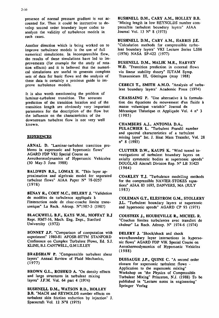
2- 10

presence of normal pressure gradient is not accounted for. Then it could be instructive to develop second order boundary layer codes to analyze the validity of turbulence models in such cases.

Another direction which is being worked on to improve turbulence models is the use of full numerical simulations. In incompressible flow, the results of these simulations have led to improvements (for example for the study of rotation effects) and it is believed that the numerical simulations are useful to generate complete sets of data for basic flows and the analysis of these data is certainly a precious guide to improve turbulence models.

It is also worth mentionning the problem of laminar-turbulent transition. The accurate prediction of the transition location and of the transition length are obviously very important parameters for the description of the flow but the influence on the characteristics of the downstream turbulent flow is not very well known.

REFERENCES ARNAL D. "Laminar-turbulent transition problems in supersonic and hypersonic flows" AGARD FDP VKI Special Course on Aerothermodynamics of Hypersonic Vehicules (30 May-3 June 1988)

BALDWIN B.S., LOMAX H. "Thin layer approximation and algebraic model for separated turbulent flows" AIAA Paper No 78-0257 (1 978)

BENAY R., COET M.C., DELERY J. "Validation de modtles de turbulence appliquts h l'interaction onde de choc-couche limite trans- sonique" La Rech. Atrosp. N01987-3 (1987)

BLACKWELL B.F., KAYS W.M., MOFFAT R.J Rept. HMT-16, Mech. Eng. Dept., Stanford University (1972)

BONNET J.P. "Comparison of computation with experiment" 1980-8 1 AFOSR-HTTM STANFORD Conference on Complex Turbulent Flows. Ed. S.J. KLINE, B J. CANlWELL, G.M LILLEY

BRADSHAW P. ."Compressible turbulent shear layers" Annual Review of Fluid Mechanics, (1 977)

BROWN G.L., ROSHKO A. "On density effects and large structures in turbulent mixing layers" J.F.M. Vol. 64 part 4 (1974)

BUSHNELL D.M., WATSON R.D., HOLLEY B.B. "MACH and REYNOLDS number effects on turbulent skin friction reduction by injection" J. Spacecraft Vol. 12 NO8 (1975)

BUSHNELL D.M., CARY A.M., HOLLEY B.B. "Mixing length in low REYNOLDS number compressible turbulent boundary layers" AIAA Journal Vol. 13 No 8 (1975)

BUSHNELL D.M., CARY A.M., HARRIS J.E. "Calculation methods for compressible turbulent boundary layers" VKI Lecture Series LS86 (1976) NASA SP-422 (1977)

BUSHNELL D.M., MALIK M.R., HARVEY W.D. "Transition prediction in external flows via linear stability theory" IUTAM Symp. Transonicum 111, Gottingen (may 1988)

CEBECI T., SMITH A.M.O. "Analysis of turbulent boundary layers" Academic Press (1974)

CHASSAING P. "Une alternative h la formulation des equations du mouvement d'un fluide h masse volumique variable" Journal de MBcanique Theorique et Appliquee Vol. 4 no 3 (1 985)

CHAMBERS A.J., ANTONIA D.A., FULACHIER L. "Turbulent Prandtl number and spectral characteristics of a turbulent mixing layer" Int. J. Heat Mass Transfer, Vol. 28 no 8 (1985)

CLUTTER D.W., KAUPS K. "Wind tunnel in- vestigations of turbulent boundary layers on axially symmetric bodies at supersonic speeds" DOUGLAS Aircraft Division Rep. No LB 31425 (1 964)

COAKLEY T.J. "Turbulence modelling methods for the compressible NAVIER-STOKES equations" AIAA 83 1693, DANVERS, MA (JULY 1983)

COLEMAN G.T., ELESTROM G.M., STOLLERY J,L. "Turbulent boundary layers at supersonic and hypersonic speeds" AGARD CP 93 (1971)

COUSTEM J., HOUDEVILLE R., MICHEL R. "Couches limites turbulentes avec transfert de chaleur" La Rech. Aerosp. No 1974-6 (1974)

DELERY J. "ShocWshock and shock waveboundary layer interactions in hypersonic flows" AGARD FDP VIK Special Course on Aerothermodynamics of Hypersonic Vehicles (1 988)

DUSSAUGE J.P., QUINE C. "A second order closure for supersonic turbulent flows - Application to the supersonic mixing" Workshop on "the Physics of Compressible Turbulent Mixing" Princeton, N.J. (1988) To be published in "Lecture notes in engineering" Springer Verlag

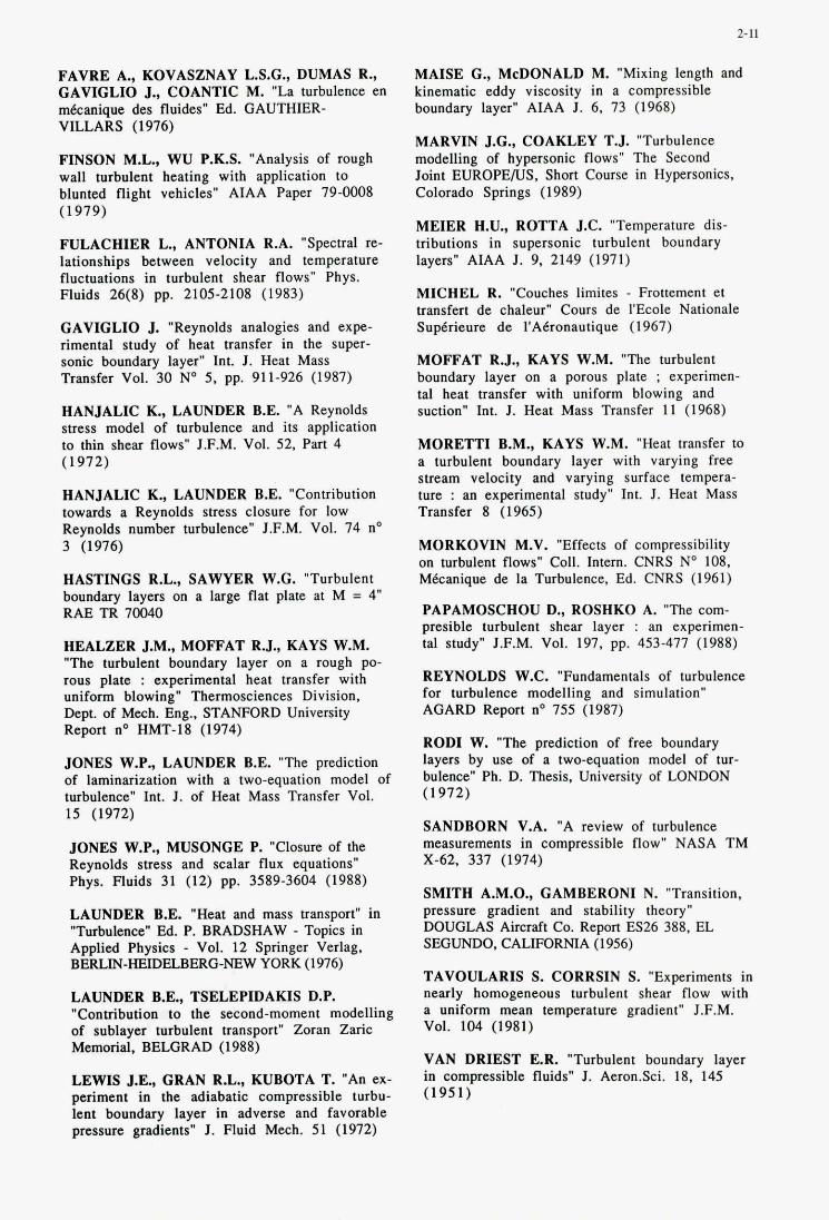
2-11

FAVRE A., KOVASZNAY L.S.G., DUMAS R., GAVIGLIO J., COANTIC M. "La turbulence en mkanque des fluides" Ed. GAUTHIER- VILLARS (1976)

FINSON M.L., WU P.K.S. "Analysis of rough wall turbulent heating with application to blunted flight vehicles" AIAA Paper 79-0008 (1979)

FULACHIER L., ANTONIA R.A. "Spectral relationships between velocity and temperature fluctuations in turbulent shear flows" Phys. Fluids 26(8) pp. 2105-2108 (1983)

GAVIGLIO J. "Reynolds analogies and experimental study of heat transfer in the supersonic boundary layer" Int. J. Heat Mass Transfer Vol. 30 No 5, pp. 911-926 (1987)

HANJALIC K., LAUNDER B.E. "A Reynolds stress model of turbulence and its application to thin shear flows" J.F.M. Vol. 52. Part 4 (1972)

HANJALIC K., LAUNDER B.E. "Contribution towards a Reynolds stress closure for low Reynolds number turbulence" J.F.M. Vol. 74 no 3 (1976)

HASTINGS R.L., SAWYER W.G. "Turbulent boundary layers on a large flat plate at M = 4" RAETR70040

HEALZER J.M., MOFFAT R.J., KAYS W.M. "The turbulent boundary layer on a rough porous plate : experimental heat transfer with uniform blowing" Thennosciences Division. Dept. of Mech. Eng., STANFORD University Report no HMT-18 (1974)

JONES W.P., LAUNDER B.E. "The prediction of laminarization with a two-equation model of turbulence" Int. J. of Heat Mass Transfer Vol. 15 (1972)

JONES W.P., MUSONGE P. "Closure of the Reynolds stress and scalar flux equations" Phys. Fluids 31 (12) pp. 3589-3604 (1988)

LAUNDER B.E. "Heat and mass transport" in "Turbulence" Ed. P. BRADSHAW - Topics in Applied Physics - Vol. 12 Springer Verlag, BERLIN-=ELBERG-NEW YORK (1976)

LAUNDER B.E., TSELEPIDAKIS D.P. "Contribution to the second-moment modelling of sublayer turbulent transport" Zoran Zaric Memorial, BELGRAD (1988)

LEWIS J.E., GRAN R.L., KUBOTA T. "An experiment in the adiabatic compressible turbulent boundary layer in adverse and favorable pressure gradients" J. Fluid Mech. 51 (1972)

MAISE G., McDONALD M. "Mixing length and kinematic eddy viscosity in a compressible boundary layer" AIAA J. 6, 73 (1968)

MARVIN J.G., COAKLEY T.J. "Turbulence modelling of hypersonic flows" The Second Joint EUROPE/US. Short Course in Hypersonics, Colorado Springs (1989)

MEIER H.U., ROTTA J.C. "Temperature distributions in supersonic turbulent boundary layers" AIAA J. 9, 2149 (1971)

MICHEL R. "Couches limites - Frottement et transfert de chaleur" Cours de 1'Ecole Nationale Suptrieure de l'A€ronautique (1967)

MOFFAT R.J., KAYS W.M. "The turbulent boundary layer on a porous plate ; experimental heat transfer with uniform blowing and suction" Int. J. Heat Mass Transfer 11 (1968)

MORETTI B.M., KAYS W.M. "Heat transfer to a turbulent boundary layer with varying free stream velocity and varying surface temperature : an experimental study" Int. J. Heat Mass Transfer 8 (1965)

MORKOVIN M.V. "Effects of compressibility on turbulent flows" COIL Intem. CNRS No 108. Mkanique de la Turbulence, Ed. CNRS (1961)

PAPAMOSCHOU D., ROSHKO A. "The com- presible turbulent shear layer : an experimental study" J.F.M. Vol. 197, pp. 453-477 (1988)

REYNOLDS W.C. "Fundamentals of turbulence for turbulence modelling and simulation" AGARD Report no 755 (1987)

ROD1 W. "The prediction of free boundary layers by use of a two-equation model of turbulence" Ph. D. Thesis, University of LONDON (1972)

SANDBORN V.A. "A review of turbulence measurements in compressible flow" NASA TM X-62, 337 (1974)

SMITH A.M.O., GAMBERONI N. "Transition, pressure gradient and stability theory" DOUGLAS Aircraft Co. Report ES26 388, EL SEOUNDO, CALIFORNIA (1956)

TAVOULARIS S. CORRSIN S. "Experiments in nearly homogeneous turbulent shear flow with a uniform mean temperature gradient" J.F.M. Vol. 104 (1981)

VAN DRIEST E.R. "Turbulent boundary layer in compressible fluids" J. AeronSci. 18, 145 (1951)

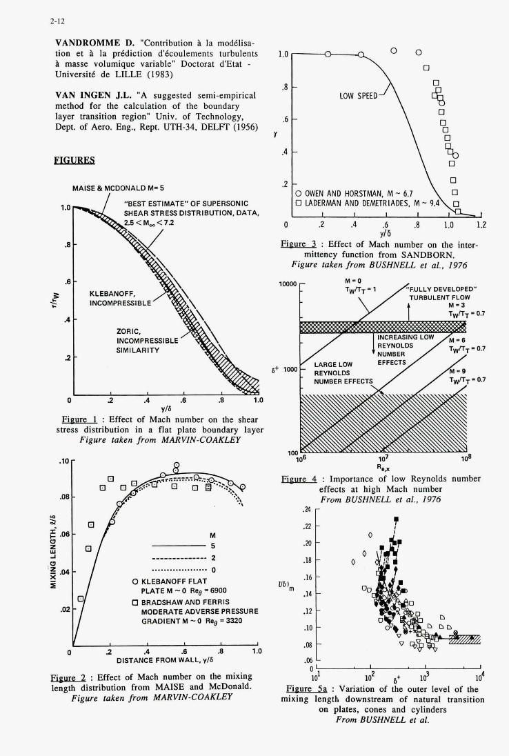
2-12

VANDROMME D. "Contribution la modtlisation et b la prgdiction d'koulements turbulents b masse volumique variable" Doctorat d'Etat - Universitt de LILLE (1983)

VAN INGEN J.L. "A suggested semi-empirical method for the calculation of the boundary layer transition region' Univ. of Technology, Dept. of Aero. Eng.. Rept. UTH-34, DEJJT (1956)

MAlSE & MCDONALD Mm 5

"BEST ESTIMATE" OF SUPERSONIC SHEAR STRESS DISTRIEUTION, DATA,

1.0

B

.(I

INCOMPRESSIBLE . IF c

.4

INCOMPRESSIBLE SIMILARITY

2

0 2 .4 .(I B 1.0 V I S

: Effect of Mach number on the shear stress distribution in a flat plate boundary layer

Figure taken from MARVIN-COAKLEY

M 5 ________------ 2 ................... 0

PLATEM-0 R 0 0 ~ 6 9 0 0

MODERATE ADVERSE PRESSURE QRADIENTM-0 Reg' W O

0 KLEEANOFF FLAT

0 BRADSHAW AND FERRIS

Y A .B .8 1 .o 0 2

DISTANCE FROM WALL, y /6

: Effect of Mach number on the mixing length dis!ihution from MAISE and McDonald.

Figure taken from MARVIN-COAKLEY

1.0 1.2 0 .2 .4 .8

Egu& : Effect of Mach number on the intermittency function from SANDBORN.

Figure taken from BUSHNELL et al., I976

FULLY DEVELOPED

NUMBER EFFEC

R.i : Importance of low Reynolds number

effects at high Mach number From BUSHNELL et al., 1976

?

0 ' I

10' 102 a+ Id lo4 I I

E~~uL.% : Variation of the outer level of the mixing length downstream of natural transition

on plates. cones and cylinders From BUSHNELL et al.

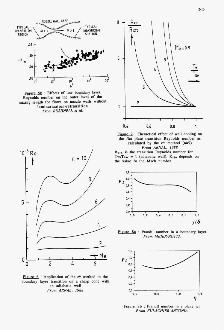
2-13

NOZZLE WAU CASE

lRA;;l;;O\wmR WPICAL TYPICAL ING

STATION

.I4 r

I I I I .02 10' ' 102 13 lo4 lo5

b'

: Effects of low boundary layer Reynolds number on the outer level of the

mixing length for flows on nozzle walls without laminarization-retransition

From BUSHNELL et al.

Rx

I t

I I I , - M e 0 2 4 6 01

: Application of the en method to the boundary layer transition on a sharp cone with

an adiabatic wall From ARNAL, 1988

"E

5 - '

l - f

0.k 0.6 0.8 1

: Theoretical effect of wall cooling on the flat plate transition Reynolds number as

calculated by the en method (n=9) From ARNAL. 1988

RXIo is the transition Reynolds number for Twmaw = 1 (adiabatic wall). Rxto depends on the value fo the Mach number

: Prandtl number in a boundary layer From MEIER-ROlTA

: I . , . , . I 0.0

0.0 0.5 1 .o 1.5

v : Prandtl number in a plane jet

From FULACHIER-ANTONIA

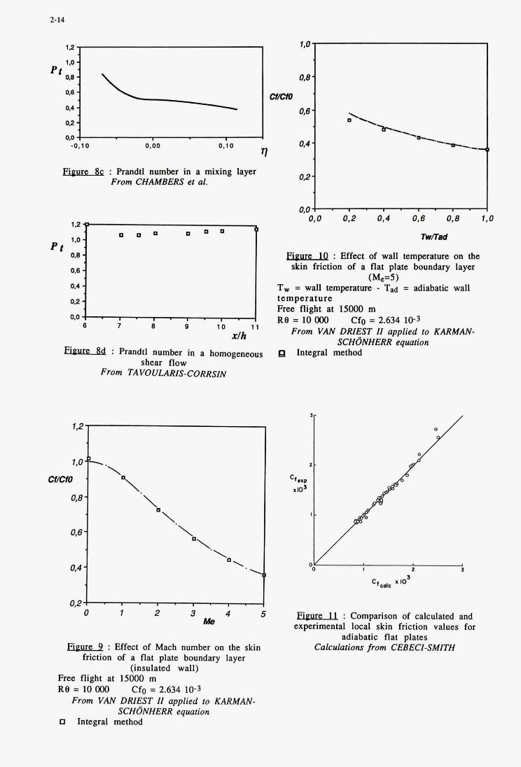
2-14

1.2-

cI/cID ‘

0.8 -

0.8 -

0.4 -

0.27

P t

I

Cf..p ’\

l,O-’-

.io3

\ I

\.

I 0 I 2 3

‘a \. 0

3 Cf0dC

‘ S . I . 0 . I .

I 7

-0.10 0.00 0.10

: Prandtl number in a mixing layer From CHAMBERS et al.

P t

xlh : F’randtl number in a homogeneous

shear flow From TAVOULARIS-CORRSIN

0 . 0 4 . . . ’ 0 . . ‘ 0.0 0,2 0,4 0.6 0.8 1

“8d

: Effect of wall temperature on the skin friction of a flat plate boundary layer

(Me=5) Tw = wall temperature - Tad = adiabatic wall temperature Frec flight at lS000 m Re = 10 Mx) Cfo = 2.634 10-3

From VAN DRIEST I1 applied to KARMAN- S C H ~ N H E R R equation

Integral method

0

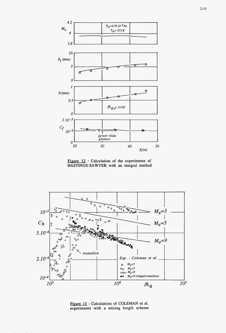
2-15

10-

ch

5.10-

2.10-

10-

3.8

2 10-3

cf 10-3 -1 omor blade

0 20 30 40 50

X(in)

: Calculation of the experiments of HASTINGS-SAWYER with 811 integral method

: Calculations of COLEMAN et al. experiments with a mixing length scheme

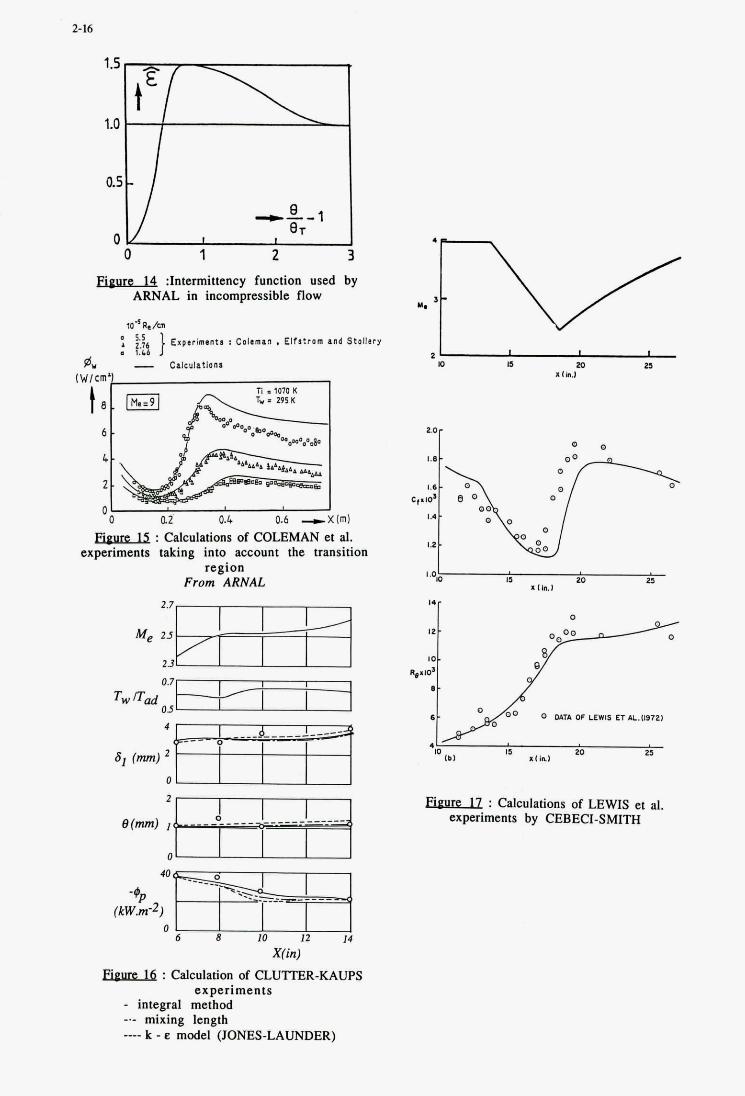
2-16

,?/ 0 1 2 3

:Intermittency function used by ARNAL in incompressible flow

U.

ro*n./ol y6 } E x p i r i m i n t i : C o l m a n , Elfatram and Stoll lry 1.b6 a - C.lc"latIon1 m I5 W U

ZIh.1 A

: Calculations of COLEMAN et al. experiments taking into account the transition

region From ARNAL

X(in) : Calculation of CLUTTER-KAUPS

experiments - integral method

mixing length k - e model (JONES-LAUNDER)

7

IO I5 Po 25 X l h . 1

1.01

: Calculations of LEWIS et al. experiments by CEBECI-SMITH

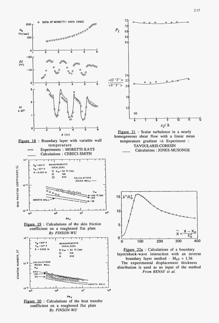
I 5 6 01 2 3 4

-20 r

I 4 5 6 01 2 3

I 2 3 4 5 6

x ( I l l

: Boundary layer with variable wall temperature

0-00 Experiments : MORE'ITI-KAYS - Calculations : CEBECI-SMITH

I 2

1

I I .I lo. lo' I)*

RE.

: Calculations of the skin friction coefficient on a roughened flat plate

By FINSON-WU I d I I

1.. m s s YEASUlLYENR

1 I I I

100 10' IO' 0'

Re*

: Calculations of the heat transfer coefficient on a roughened flat plate

By FINSON-WU

L

2-17

(a)

6 I ~ 9 i o n a xl l h

: Scalar turbulence in a nearly homogeneous shear flow with a linear mean

temperature gradient --A Experiment : TAVOULARIS-CORRSJN

- Calculations : JONES-MUSONGE

: Calculations of a boundary layer/shock-wave interaction with an inverse

boundary layer method - Me0 = 1.36 The experimental displacement thickness

distribution is used as an input of the method From BENAY et al.

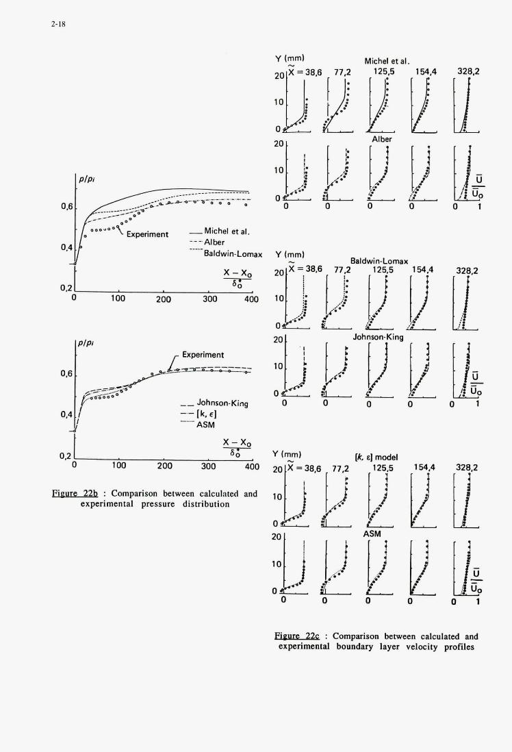
2-18

I PIPI

x-xo 0.2 -G-

0 100 200 300 400

YP’ ,- Experiment

x-xo %-

0 100 200 300 400 0 2

&ur~Z& : Comparison between calculnted and experimental pressure distribution

Y (“1 Michel et al.

0 1

0 1

328.2

I I

&UILZ& : Comparison between calculated and experimental boundary layer velocity profiles

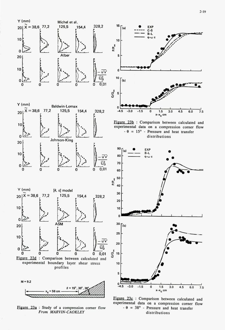
2-19

30

25

20

8

a % a 1 5 -

10

Michel et al.

?bl

- -

-

Y (mml - Baldwin-Lcmax 20

10

0 .,. 20

0 ' 0 0 0 0

[ :.

6 - U'"'

0 0.01

Y (mml [k, el model . .

77.2 125.5 lly1,4 t328,2 I

: Comparison between calculated and experimental boundary layer shear stress

profiles

: Study of a compression comer flow From MARVIN-CAOKLEY

4 .5 -3.0 -1.5 0 1.5 3.0 4.5 6.0 7.5 x-xc cm

&u.GLlb : Comparison between calculated and experimental data on a compression comer flow

- 9 = 15' - Pressure and heat transfer distributions

10

0 :U,, , ,

st 0 4.5 -3.0 -1.5 o 1.s 3.0 4.5 6.0 7.5 . ..

x-xc un

: Comparison between calculated and experimental data on a compression comer flow

distributions - e = 38' - Pressure and heat transfer

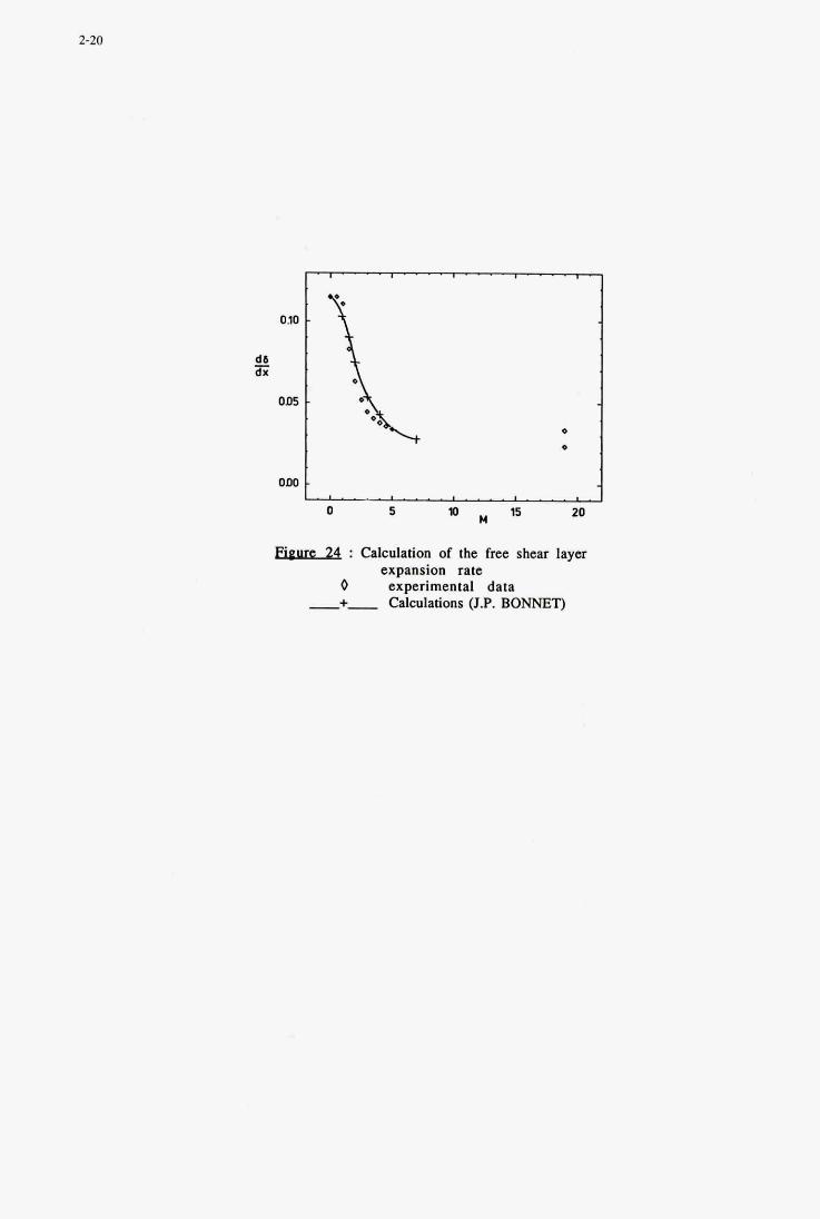
0.10

dK a;; OD5

OD0

0

*

0 5 " w 15 20

Eigu~24 : Calculation of the free shear layer expansion rate

0 experimental data -+- Calculations (J.P. BONNET)

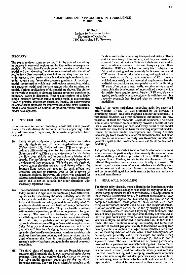
3-1

SOME CURRENT APPROACHES IN TURBULENCE MODELLING

W. Rodi Institute for Hydromechanics

University of Karlsruhe 7500 Karlsruhe, F.R. Germany

SUMMARY

The paper reviews some recent work in the area of modelling turbulence in near-wall regions and by Reynolds-stress-equation models. Various low-Reynolds-number versions of the k-e model and their damping functions are examined with the aid of results from direct numerical simulations and they are compared with respect to their performance in calculating boundary layers under adverse and favourable pressure gradients. A two-layer model is presented in which near-wall regions are resolved with a one-equation model and the core region with the standard k-e model. Various applications of this model are shown. The ability of the various models to simulate laminar-turbulent transition in boundary layers is discussed. Recent applications of a fairly simple, standard Reynolds-stress-equation model to two complex flows of practical interest are presented. Finally, the paper reports on some recent proposals for improved Reynolds-stress-equation models and provides an outlook on possible future turbulence- model developments.

1. INTRODUCTION

In conventional turbulence modelling, whose task it is to provide models for calculating the turbulent stresses appearing in the Reynolds-averaged equations, three main approaches have emergd

(i) Fairly simple eddy-viscosity models, which are either entirely algebraic and of the mixing-lenth-model type (Cebeci-Smith [ 11, Baldwin-Lomax [2]) or employ an ordinary differential equation for the maximim shear stress (Johnson and King [3]) are used extensively for calculating the flow over airfoils and turbomachinery blades at all speeds. The usefulness of the various models depends on the degree of flow separation. While the entirely algebraic models cannot simulate transport and history effects, the Johnson-King model can account for such effects and therefore appears to perform best in the presence of separation regions. However, this model was designed for extemal aerodynamic flows with relatively small separation zones and is not so suitable for other situations with massively separated flow.

(ii) The second main class of turbulence models in practical use today are the k-e-type models employing two differential equations for calculating the eddy viscosity, one for the velocity scale and the other for the length scale of the turbulent fluctuations. k-e-type models are widely used for practical calculations and are built into many commercial general-purpose CFD codes. They can handle situations with massive separation; yet there is no guarantee for good accuracy. The use of an isotropic eddy viscosity, establishing a close link between the turbulent stresses and the strain rate, is probably too simple for highly non- isotropic situations prevailing in flows with complex strain fields. Most practical k-e model calculations are still carried out with wall functions bridging the viscous sublayer. but recently also low-Reynolds-number versions resolving this sublayer have become popular, and these versions must be used whenever the flow is transitional. Considerable research activity has been going on in the area of near-wall modelling.

(ii) The third class of models in use are Reynolds-stress- equation (RSE) models also known as second-order closure schemes. They do not employ the eddy-viscosity concept but solve model-transport equations for the individual Reynolds stresses. They are better suited for complex strain

fields as well as for simulating transport and history effects and the anisotropy of turbulence, and they automatically account for certain extra effects on turbulence such as due to streamline curvature, rotation. buoyancy and flow dilatation. RSE models have recently been subjected to fairly wide testing and are presently built into commercial CFD codes. However, the main testing and application has been restricted to fairly basic versions of RSE models which do not satisfy certain theoretical requirements like the realisability conditions and compatability with the limiting 2D state of turbulence near walls. Another active area of research is the development of more refined models which do satisfy these requirements. Further, RSE models were applied so far mainly in connection with wall functions, but recently research has focused also on near-wall RSE modelling.

Much of the recent turbulence modelling activities described briefly under (ii) and (iii) was prompted by the increase in computing power. This also triggered another development in turbulence research, as direct numerical simulations are now possible, at least for moderate Reynolds numbers. The direct simulations performed to-date already provide a wealth of data that allow the checking of each and every detail of the model proposals and may form the basis for devising improved models. Hence, turbulence-model development and testing benefits increasingly from the direct numerical simulation data, but since these are so far restricted to fairly low Reynolds numbers, the greatest impact of the direct simulations was so far on near-wall modelling.

The present paper describes some recent developments in areas where research is particularly active, namely the areas of near- wall modelling and the application of basic RSE models to complex flows. Further, trends in the development of more refined Reynolds-stress closures are briefly discussed. Of necessity, only some areas of recent turbulence-modelling work can be covered, and the paper focuses on incompressible flow and on the modelling of Reynolds stresses (rather than turbulent heat and mass fluxes).

2. NEAR-WALL MODELLING

The simple eddy-viscosity models listed in the Inaoduction under (i) resolve the viscous sublayer near walls by relying on the van Driest damping model for the eddy viscosity. The application of these models is restricted mainly to extemal aerodynamic flows without massive separation. Dictated by the limitations of computer resources, most practical calculations with more complex turbulence models such as k-e- and Reynolds-stress- equation models were carried out so far by bridging the rather thin, viscosity-affected near-wall layer by wall functions. The areas of steep gradients in this layer were thereby not resolved as the first grid point away from he wall was placed outside the viscous sublayer. As described in some detail in [4] for the k-e model, the wall functions relating the velocity and turbulence quantities at the first grid point mainly to the friction velocity lean heavily on the assumption of a logarithmic velocity distribution and of local equilibrium of turbulence. These assumptions are certainly not generally valid, for example not when strong secondary flows extend into the sublayer [SI and also not in separated flows. The wall functions are of course particularly unsuited for separation and reattachment regions. Due to recent increases in computing power, the necessity to use wall functions is now much reduced, and considerable activity was recently directed towards testing and developing low-Reynolds-number models for simulating the turbulent processes very near walls. In the following, some of these activities will be described for k-e- type models. It should be mentioned in this context that for

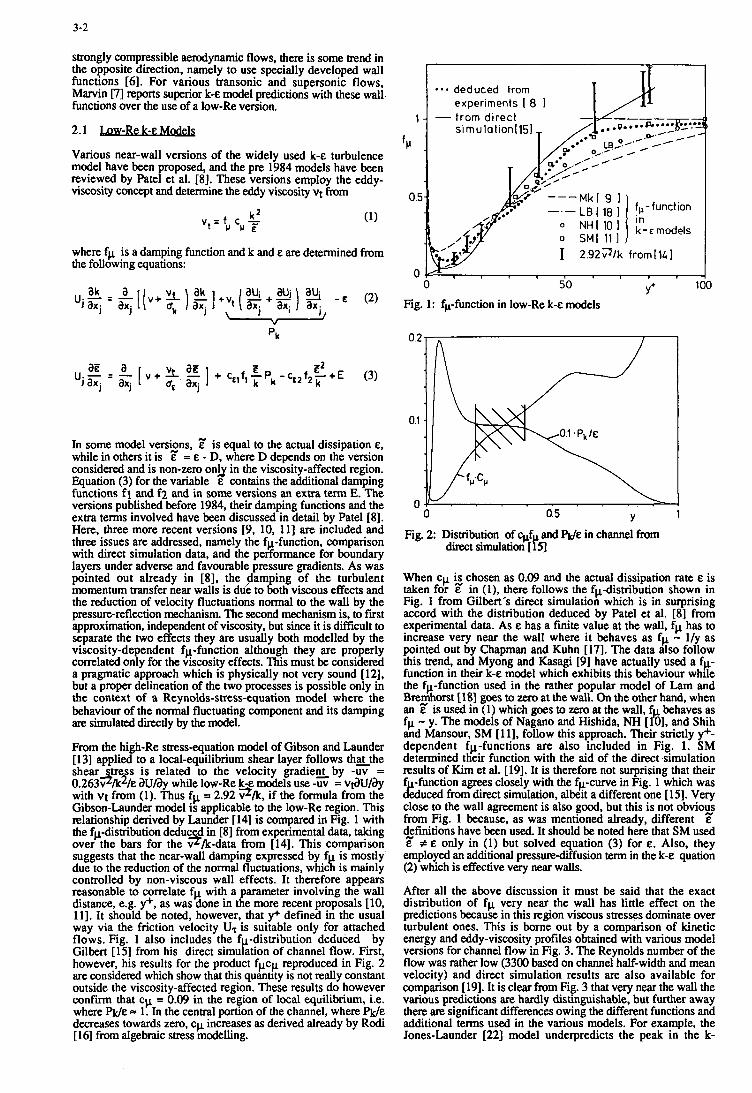
3-2

0.2-

0.1 .

strongly compressible aerodynamic flows, there is some trend in the opposite direction, namely to use specially developed wall functions [6] . For various transonic and supersonic flows, Marvin [7] reports superior k-E model predictions with these wall functions over the use of a low-Re version.

2.1 L g w R e k E w - - Various near-wall versions of the widely used k-E turbulence model have been proposed, and the pre 1984 models have been reviewed by Patel et al. [8]. These versions employ the eddy- viscosity concept and determine the eddy viscosity vt from

k 2 IJ P E v t = f c -

where fp is a damping function and k and E are determined from the following equations:

- = - [ [ v + p ) & ] + v t ( ~ + ~ ) ak a 2 - E (2) ‘i axj axj

V

‘k

In some model verskns, z is equal to the actual dissipation E, while in others it is E = E - D. where D depends on the version considered and is non-zero on9 in the viscosity-affected region. Equation (3) for the variable E contains the additional damping functions f i and f2 and in some versions an extra term E. The versions published before 1984, their damping functions and the extra terms involved have been discussed in detail by Patel [8]. Here, three more recent versions [9, 10, 111 are included and three issues are addressed, namely the fp-function, comparison with direct simulation data, and the performance for boundary layers under adverse and favourable pressure gradients. As was pointed out already in [8], the amping of the turbulent

the reduction of velocity fluctuations normal to the wall by the pressure-reflection mechanism. The second mechanism is. to fist approximation. independent of viscosity. but since it is difficult to separate the two effects they are usually both modelled by the viscosity-dependent fp-function although they are properly correlated only for the viscosity effects. This must be considered a pragmatic approach which is physically not very sound [12]. but a proper delineation of the two processes is possible only in the context of a Reynolds-stress-equation model where the behaviour of the normal fluctuating component and its damping are simulated directly by the model.

From the high-Re stressequation model of Gibson and Launder [13] applied to a local-equilibrium shear layer follows thgthe shear tre s is related to the velocity gradientby -uv =

with vt from (1). Thus fp = 2.92 ?/k, if the formula from the Gibson-Launder model is applicable to the low-Re region. This relationship derived by Launder [ 141 is compared in Fig. 1 with the fp-distribution deduc in [8] from experimental data, taking

suggests that the near-wall damping expressed by f is mostly due to the reduction of the normal fluctuations, whici is mainly controlled by non-viscous wall effects. It therefore appears reasonable to correlate fp with a parameter involving the wall distance, e.g. y+, as was done in the more recent proposals [lo, 111. It should be noted, however. that y+ defined in the usual way via the friction velocity UT is suitable only for attached flows. Fig. 1 also includes the f distribution deduced by Gilbert [15] from his direct simukion of channel flow. First, however, his results for the product fpcp reproduced in Fig. 2 are considered which show that this quannty is not really constant outside the viscosity-affected region. These results do however confirm that c p = 0.09 in the region of local equilibrium, i.e. where WE = 1. In the central portion of the channel, where WE decreases towards zero, cp increases as derived already by Rodi [ 161 from algebraic stress modelling.

momentum transfer near walls is d 4 e to both viscous effects and

0 .263~ w At /E aU/ay while low-Re k-e models use -uv = v$U/ay

over the bars for the v 9 At-data from [14]. This comparison

a - . deduced trom experiments I 8 1

1 - - trom direct

I 2.927lk fromIll1

Y+ 0 50

Fig. 1: fp-function in low-Re k-E models

O J 0 1 0.5 Y

I

Fig. 2: Distribution of cpf and %/E in channel from direct simulation [ f5]

When cp is chosen as 0.09 and the actual dissipation rate E is taken for i? in (1). there follows the fp-distribution shown in Fig. 1 from Gilbert’s direct simulation which is in surprising accord with the distribution deduced by Patel et al. [8] from experimental data. As E has a finite value at the wall, fp has to increase very near the wall where it behaves as fp - l/y as pointed out by Chapman and Kuhn [17]. The data also follow this trend. and Myong and Kasagi [9] have actually used a fp- function in their k-e model which exhibits this behaviour while the fp-function used in the rather popular model of Lam and Bremhorst [18] goes to zero at the wall. On the other hand, when an z is used in (1) which goes to zero at the wall, fp behaves as fp - y. The models of Nagano and Hishida, NH [lo]. and Shih and Mansour, SM [ 111. follow this approach. Their strictly y+- dependent fp-functions are also included in Fig. 1. SM determined their function with the aid of the duect4mulation results of Kim et al. [19]. It is therefore not surprising that their f -function agrees closely with the fp-curve in Fig. 1 which was &uced from direct simulation, albeit a different one [15]. Very close to the wall agreement is also good. but this is not obvioks from Fig. 1 because, as was mentioned already, different E *finitions have been used. It should be noted here that SM used E f E only in (1) but solved equation (3) for E . Also, they

employed an additional pressurediffusion term in the k-E quation (2) which is effective very near walls.

After all the above discussion it must be said that the exact distribution of fp very near the wall has little effect on the predictions because in this region viscous stresses dominate over turbulent ones. This is borne out by a comparison of kinetic energy and eddy-viscosity profiles obtained with various model versions for channel flow in Fig. 3. The Reynolds number of the flow was rather low (3300 based on channel half-width and mean velocity) and direct simulation results are also available for comparison [19]. It is clear from Fig. 3 that very near the wall the various predictions are hardly distinguishable, but further away there are significant differences owing the different functions and additional terms used in the various models. For example, the Jones-Launder [22] model underpredicts the peak in the k-

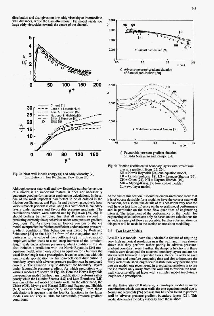
3-3

distribution and also gives too low eddy vipcosty at inmmdiate wall diswces. wbile the b-Bremhors l [ lS] modcl yiclds too largeeddyviscositiesmwardstheccnatofthechaMeL

a) Advenc-p"egn&nt siprption of Samuel and Joubat 1301

I

0 50 100 150 200 Y+

Chien121 1

----- Lam h Bremhmt 1181 Nagono 8 Hishidall01 _a---

-

15 l o

0 40 80 120 160 Y+

Fig. 3: Near-wall kinaic enagy Q and cddy-viwx (vd distributions in low Re channel flow. from I 28 1

Although -t near-wall and low-Rcynolds-numbcr behaviour of a model is M important feature, it does not necessarily g u a I a n t e e g o o d p e r f n m a n c e i n e n ~ g ~ n s . l n t h e s e , one of the most important parameters to be calculated is the friction coefficient cf, and Figs. 4a and b show rcspstively how wious modclspcrform in calculating this wefficicnt in boundary layers undcr adverse and favourable pressure gradients. The calculations sbown were carried out by Fujisawa 125,261. It should perhaps be mentioned fvst that all modcls succeed in pred@ng-tIythecfkbaviourunderzcro~gradient condmons. Fig. 4a shows that all low-Re versions of the k-e model wcrprcdict the friction wefficient under adverse pres"-

ent conditions. This behaviour was trsced by Rodi and P cheuerer 1231 to the high-Re-form of the e-cqUation (and in particular to the value of the wefficient cc1 in this equation) employed which leads to a too swp mcrcasc of the turbulent length scale luder advase pressure-gradient conditions. Fig. 4a also includes a prediction with the Norris-Reynolds 1241 one- equation modcl. which only solves an equation fork but uws the usual lincar length-de prescription. It cm be san that with this length-scale spcciscation the friction-cocfficient distribution in boundary layers with advase pressure gradient can be pradictcd EoIIcctly. The situation is quite different for boundary layers under favourable pressure gradient, for which predictim with various models arc sbown in Eg. 4b. Here the Norris-Reynolds onequation model (without any modification) @oms rathex poorly wbile thc Laundcr-Slumns U) and Lam-BnmhoRI (LE) venionsotthck-emodel&fairlywell.On~othahand,the Chien (CH), Myong and b g i (MK) and Na and Hishida 0 models also overpredict cy c o n s i d c n r From thew calculations it appears that the low-Re functions in the latter modcla arc not very suitable for favourable pressuregradient conditions.

aooz I I 0.1 az 01 0.4 as

a (ml

b) F a v o u r a b l e - p e n t siluadon of Badri Narsyaran and Rsmjcc I311

Fig. 4 Friction wefliient in l"y layers with sueamwise plcssun gradims f" I=. 2 4 ; NR = NarieRcynoldr [U] OoC-equBtiM modcl. LB=Latn-B"t[lSl.LS=Lauodcr-Sllllma[36l, CH = Chicn 1211, NH - Nagmo-Hishida 1101, MK = Myong-Kasagi I91 low-Re-k-e models. 2L = twelayer modcl,

At the end of this section it should be emphaaizcd oncc molt that it is of course desirable for a model to have the "ct ncar-wall behaviour, but also that the &tails of this behaviour vcry lfcBT the wall haVC in fact liale Mmffi on t b e 0 v d m o d e l p " m a and in particular on the man-flow quantities of engiaccring intextst. The judgemnt of the peaormancc of the model for enginazing calculations can only be based on tcst calcvlations f a as wide a variety of flows ss possible. F u r t h ~ substantiation on this point wiU bemade in the s tdonon uansiticm modclling.

2.2

Low-Re k-e models have the undcshbk feature of requiring very bigh n d c a l resolution near the wall, and it was shown above that they paform rather poorly in adverse-pressuregradient b o u w layers. Funher, the g functions in these models were developed for attached ISY~andSrenOt always well behaved in separated flows. Hence, in adex to save grid points and U" wmputing tim and also to introduce the fairly well established length-scalc disaibution very ncar the wall into the model, OIICIwent tnndinpnctical d e s is to usc

wall v id ty4 fec t ed layer with a simpler model involving a kngth-salc plwxiption.

the k-E modcl only away from the wall and torwolvc the m-

3""" " i r a n d R c ~ [ 2 4 ] k u u s c t h i a h s s ~ f w n d t o well in adverse-prcssun-gradient boundary layers 12 I Thu modeldemrmms . thecddyvi.maityfiwntbcbcrclatiole

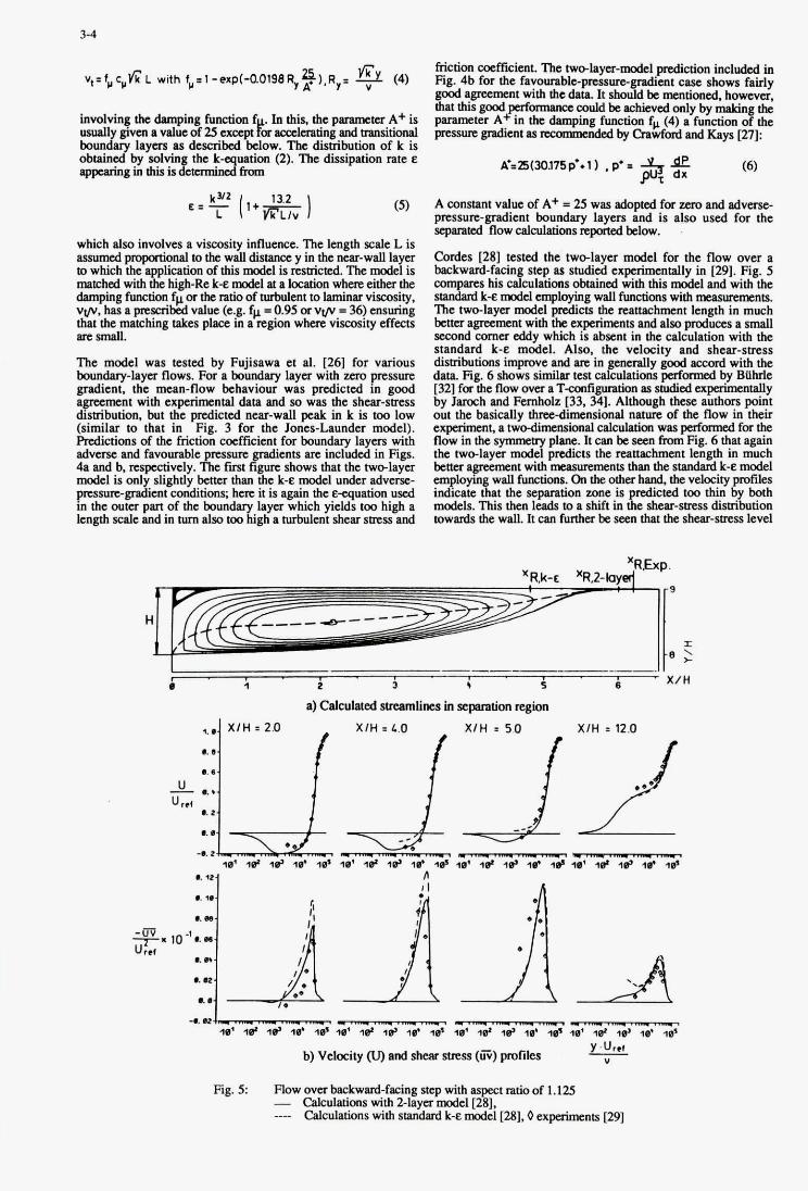
3 4

Vt i

involvinq the damping f . In this the p . n " A+ is l p M I a ~ u c ~ ~ e x c e p k r ~ a n d a n d s i t i o n a l

bo% laycrs as detctibd below. The distribution of k is obtain bysolvia thek uation(Z).Tbedissipntionratee lpparing in this is

which also involves a viscasity influcace. The len& scale L is assuaxdpropartional m the wall dismncc y in the near-wall laye to which the application of this modcl is muictcd Thc modcl is matchedwiththe high-Re k e d a t a M o n whaceithathe damping f p o r t h e n t i o o f t t to laminar viscosity, v p . has a pscnhcd value (e.g. fp = 0.95 or v p = 36) cnsllriag that the matching taLcs placc in arcgion what viscosity effects s r c d

The model was tested by Fujisawa et al. [2q for various boundary-layer flows. For a boundary layer with EQD pssm gradient. the "-flow behaviour was predicted m good ape" with experimental data and so was the shear-stress dtsrribuuon. but the predicted nuu-wall peak in k is too low (similar to that in Fig. 3 for the Jones-Launder model). Redictions of the fiction wcfficicnt for boundary layps with advase and favourable p" cnts an includcd in Figs.

model is only slightly bum than the k-e modcl undcr adverse

in the outer pm of the y l a y e r which yields too high a length scale and in turn llso tca gh a turbulent shurstress and

4a and b, respectively. The first tP g m shows that the w l a y c r

psure-lgsdimt cooditions; hnc it is again me e-quation uscd

Cordcs [281 tested the two-layer model for the tlow wer a backwnrd-facin step as studied experimCnelly in [29]. Fig. 5

s"d k e model cmployhg wall funuicms with nra"~. Ihc two-layer model predicts the reattachment length in much bum a g " t with theexpnimmrs andllso prod- a small sccond corner eddy which is absent in the calculation with the standard k-e model. Also, the velocity d shear-stress disaibutionsimproveandarcin YgOOdaccordwiththC dataFig.6showssimilatcst [32] forthe flow ova aT.wn6gumion as aatdicd Y by Jamch aad Fcmholz r33.341. Although tbcsewmt out the basically thne-dimensional nmtre of the flow in their cxpcrirrmsatwo-dimeesionalcalculsnm . wasperfonncdforthe flow in the sy"cayplanc. It can be seen fmn Fig. 6 that ngah the two-layer model predkts the reattachment length in much bettaagremmtwith " ~ L L S thm the standmd k-emodcl

3- Lt the separation m e is predicted too thin rZ modcls. This thcn luds ma shift in the shur-suess didbution towards the wall. It can huthcr be seen that the shear-stress level

comparcshis L o b u i n c d w i t h this modeland with the

oyin w a l l f u o c t i o n r . ~ t h e t h c ~ t h e n b c i t y

9

I. I X I H E L.0 X I H = 5.0

f X I H = 12.0

-am; I#' lo' 1e 1.. I# ,z-zTTz I4 I# ,e-

% U b) Velocity (U) and shear (LuI?ss (E) pmtilur

Fig. 5 Flowoverbaekwsrd-faCingstepwithaspMrstiOof1.125 - calculrrions with >layer modcl [Z], -- Gal- with standmd k-e model [281.0 ex&nc.nts [29]

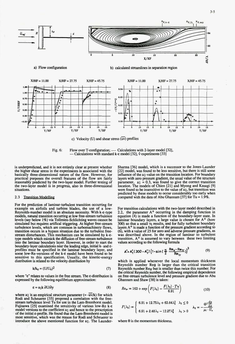
3-5

xR.k-e ‘R.21 ‘R.nP

a) Flowmn!iguration

Fig. 6: Flow over T-mnliguration; - Calculations with 2 - h ~ model [321, --calculations with standard k-e model I32J.O experiments 1331

is undaprcdictcd, and it is not entirely clear at present whether the higher shear smss in the expaimnts is associated with the basically three-dimensional nature of the flow. However. for practical purposes the overall features of the flow are fairly reasonably predicted by the twc-layer model. Funher testing of the hvc-layer model is in pmgress, also in three-dimensional situations,

2.3

F a the predictioo of laminar-turbulent transition occurring for example on airfoils and turbine blades, the use of a low- Reynolds-number model is an absolute nsessity. With Le-type model$ nahlral transition d g at low frcc-sueam turbulence levels (say below 1%) via Tollmien-Schlichting waves cannot be simulated but q u i r e s artifical triggering. At higher free-saam turbulence levels, which are “non in turbomachinery flows, wnsition occurs in a bypass situation due to the turbulent freestream disturbances. Thts mechanism can be simulated by k-e- typc models which ” i c k thc di f fush of fmestrcam turbulence into the laminar boundary layer. However, in oder to s t a t the boundary-lay= calculations near thc lcading edge, initial k- and e- profiles must be spciiied in the laminar boundary layer, and so= low-Re-versions of the k-e model have been found to be sensitive to this specification. Usually. the kinetic-energy distribution is related to the velocity distribution by

..

(7)

wberc “e” relates to values in thc fru stlcam Ihc E-distribution is expressed by thc following equilibrium approximation:

E = alk au& wherc a1 is an empirical s m c m paramcar (= -ii/k) f a which Rodi and Schcuacr 1351 proposed a comlation with the hee- sfMm ~ u l e a c c level Tu for ux in the Lam-Bmnhom d e l . Pujisarva 1251 examined the sensitivity of various low-Re k-e modcl v&om to the wcfficienl ai and hcnce to the prescription of the initinl e-pmfde. He found that thc Lam-Bmnhorst modcl is most sensitive, which was the redson f a Rodi and Scheuacr to i n d u c e the above mentioned function for ai . The Launder-

Sharma [36] model, which is a succesm to the Jones-Launder [22] model, was found to be less sensitive, but there is still ~ o m c influence of the ai-value on the transition location. For boundary layers with zero prrssun @ens the usual value of the smcture parameter. a1 = 0.3, was found to give the correct transition location. The models of Chien [21] and Myong and Kasagi [91 wcm found to be insensitive to the value of al. but mansition was predicted by these models to occur mnsiderably too early when compared with the data of Abu Ghannam [37] for Tu = 1.9%.

For wnsition calculations with the twc-layer model desrribcd in 2.2, the parameter A+ occurring in the damping function in equation (4) is made a function of the boundary-layer state. In laminar boundary layers. a largc value is chosen for A+ (hem 300) so that a small vt results, and for fully turbulent boundary layers A+ is madc a function ofthe pnssun gradient d g to (6). with a value of 25 for mo and advasc prcssun gradicnu. as was described above. In the region of laminar to turbulent transition. A+ is assumd to vary between thex two limiting values sccading to the following formula

which is applied whenever the local momentum thickness Reynolds number Reg is larger than the critical transition Reynolds number Rcf, but is d e r than twice this number. For the critical Reynolds number, thc following empirical dependence on hee-strram turbulence level and pressure gradient due to Abu Ghanaam and Shaw 1381 is taken:

Ree = 163 + ezp ( F(Xa) - F(A”.Tu) 6.91 (10)

6.91 + 12.75Az + 63.w A, 5 0

6.91 + 2.18A1 - 12.27g A, > 0 At = -A

PI ’ U. 1 F ( M =

where Cl is the “enturn thickness.

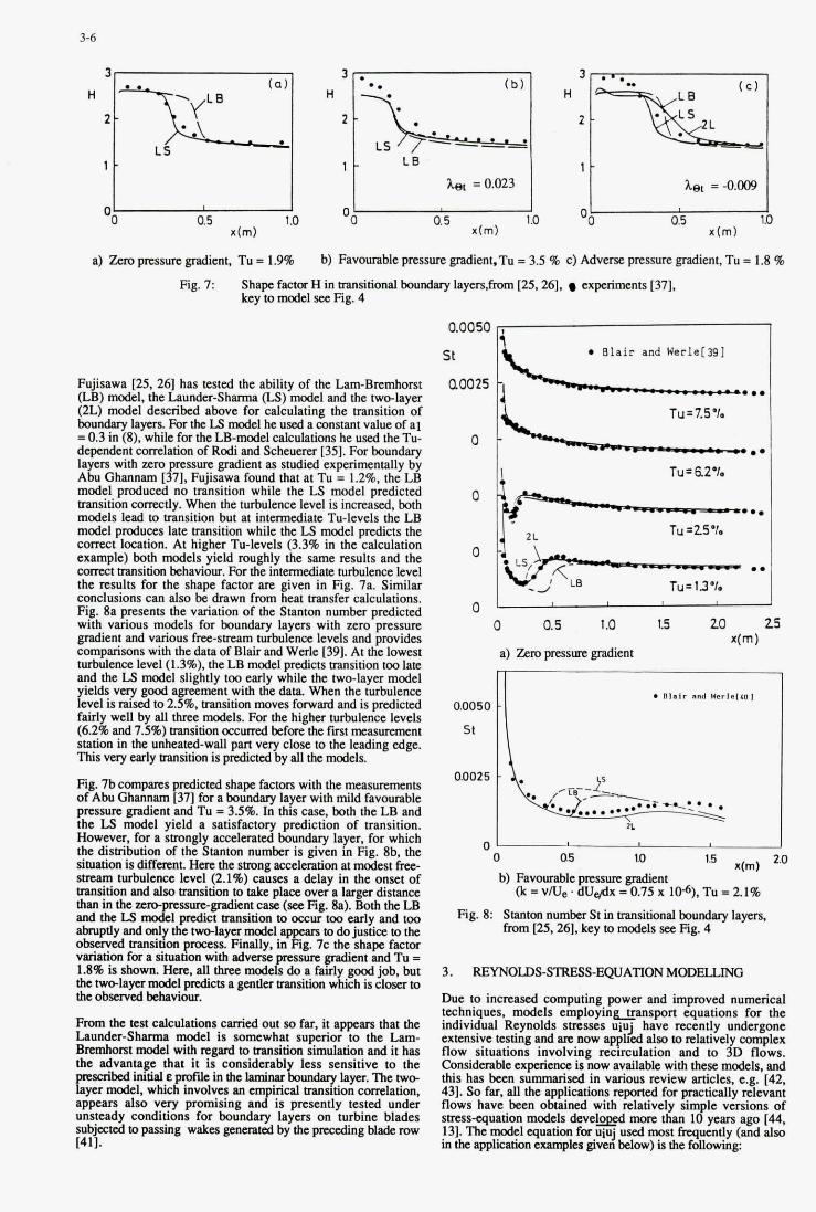
3-6

L B

let = -0.009

x(m) 0.5 1 a

x h )

a) zero pssure gradient, TU = 1.9%

Fig. 7:

b) Favourable pressure gradient.Tu = 3.5 % c) Adverse pressure gradient, Tu = 1.8 %

Shape fanor H in transitional boundary layers,fmu [25.26l. experiments 1371, key tomodel set Fig. 4

Fu'isawa [Z. 261 has tested the ability of the Lam-Bretnhmt d) model. the Laundcr-Shamu (LS) model and the two-layer (2L) model described above for calculating the transition of boundary lam For the LS modcl he used acollstsDt value of a1 = 0.3 in (8). whilc for the LB-model calculations he used the Tu- dependent axrelation of Rodi and Scheucrcr [35]. For boundary layers with zero pressure gradient as studied experimentally by Abu Gbannam [371, Fujisawa found that at Tu = 1.2%. the LB model p m d u d no transition while the LS model predicted transition comctly. When the turbulence level is incnased, both models lead to transition but at in- ' Tu-levels the LB modcl produccs late transition while the LS model predicts the c o n a t location. At bigha Tu-levels (3.3% in the calculation example) both models yield roughly the same results and the COmEt transition hchaviour. For the intermcdistc turbulence Iml the rcgults for the shape f acm arc given in Fig. 7a Similar conclusions can also he h w n fmm h u t transfer calculations. Fig. 8a presents the variation of the Stanton number predicted with various models for boundary layers with zero pressure gradient and various fi'c&sacam nubdencc levels and provides comparims with the data of Blair and Wcrle [39]. At the lowest turbulcncclcvcl(1.3%),theLBmodclprcdictstransitiontoolace and the LS model slightly too early whilc the two-layer model yields vcry @ agreement with the data When the turbulence level is raised to 2.5%. transition moves forward and is predicted fairly well by all thrcc modcls. For the bigha turbulence levels (6.2% and 7.5%) traositioD o~cumd befm the first " n t station in the unheated-wall part vcry close to the leading edge. This very early nansition is predicted by all the modcls.

Fig. 7b compares predicted shape factors with the mcasuremnts of Abu Ghannam [371 for a boundary layer with mild favourable prcssure gradient and Tu = 3.5%. In tlus CBJC, both the LB and the LS model yield a satisfactory prediction of transition. However, for a saongl accelerated boundary layer, for which the distribution of the !knton number is given in Fig. 8b. the siautioll is~~tHcrcthestrongacceleratioaatmodest~ m c ~ m turbulence level (2.1%) causa a delay in the onset of mnritioa and also u a n s i h ~ to aLc phccovera largcsdistance m a n i n t h e m gradient cast. (KC Fig. Ea). Both the LE and the Ls InlJzza transition m MTurtoo early and too h p t l y r u d d y the ~ l a y c r m o d c l appcars to do justice m the obaa-ved d h o n v s a . F W y . in Fig. 7c the shape fac ta variation fora situntrw with sdvac 8 1 1 1 ~ glpdiwlt and Tu = l . ~ ' k i s s h o a m . ~ c r c . a l l l l n e e ~ a ~ y g o o d j o b . b u t the~layermcddpredictsaga~tlertransition whichisclosum the obaa-ved behaviour.

From the test calcvlations c a n i d out so far, it appears that the

a p w also vcry promising an IS presently tested under unsteady conditions for boundary layers on turbine blades s u b j d mpkuins wakes g e n d by thepnading bladerow ~411.

e Blair and Werle[391 st a0025

I! Tu=6.2%

Tu =25% 0

-d Tu-13%

0 0.5 1.0 l.s 20 0

25

O l+c7*::

01

' 0 as (0 1.5

b) Favourable pressm gradicnt & = V/lJe. dU& = 0.75 x 106). Tu = 21%

I

Fig. 8: stanton numbcr st in transitional bourdary layers. hom [U, 261, key to models sec Fig. 4

3. RNNOIDS-sTREsS-EQUATION MODELLING

Due to incrcascd computing power and improved numerical nchniqucs, models employingtranspon equations for the individual Reynolds stre81ts uiuj have recently undergone cxfc118iyc testing and pn now ppp'lcd rlso to rclltivel annplex flow situations involving recuculation and to 3y D flows. CMlsidaable expaicna ia now avajlable with these models, and this has bee0 summarised in various review articles, e.g. [42, 431. So far, all the applicltions rcportcd for practically relevant flows have been obtained with relatively rim IC versions of messquation ~ C V ~ I I m m than IB- ago 144. 131. The modcl & foa uiuj used mpst hpa~t!~ (and ala0 in the a € l p m exampled below) UI the fdowmg:

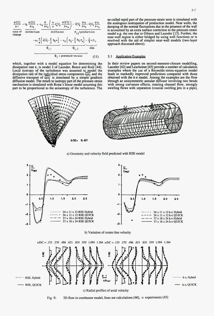
9-7

d l e d rapid pan ofthc pressun-saain term is simulated with the analogous isompation of Pmduction d e l . New walls tbe damping of thc normal flucb~hons due to thc pp.esence ofthe wall is accounted by an exha surface eorrcction to the pressure-sunin d e l e.g. thc one due to Gibson and Launder [131. Funhcs. the nur-wall region is either bridged by using wall functions or is resolved with the aid of simpler near-wall models ( w l a v e r approach discussed above).

(1 1) o,, i pre?i--s.btTaln

which, together with a model equation for determining the dissipation rate e, is modcl 2 of Launder, Rcsc and Rodi [U]. Local isotmpy of the turbulence was assumed t o s e l the dissipation rate of the individual mess components uiuj and the diffusive mnspon of is simulated by a simple gradient diffusion modcl. The return to isotropy pan of tbcpmmre-saain mechanism is simulated with Rom's lincar modcl assuming this pan to k proportional to the anisotropy of thc nubuleoa. Thc

. . 3.1 &&x

In their review papcrs on =cud-mommt-closure modclling. Luudcr [421 and Lwchzina [431 pmvidc a number of calmlation examples where the usc of a Reynolds-stress-equation modcl

obtsincd with thc k-e modcl. Among tbc exampks arc the flow e g h M anisymmcuic annular difi-usor involving hvo bends anth strong curvature effects. rotating channcl flow, strongly swirling flows wirh separation (coaxial swirling jers in a pipe),

lcads to marLcdly improved prcdinions compared with thosc

a) Geomay and velocity field predincd with RSE model

. ._. . - - 24 x I I x l2RSEHyMd 24 x 11 x 12RSEQUICK _-- 37 x IS x 24 RSE Hybrid 3 7 x ISx24RSEQUICK

---_ - -3

3 U

I.

------ 'JAxIlx12k~Hybrid ---- 24 x 11 x 12 k-e QUICK --- 37 x 18 x 24 k-eHvbdd 9 - 37 x IS x 241

" t -3 1 CQ Q ~ C K

b) V d m of cenmline velocity

NE€!= ,135 ,270 ,486 ,621 ,824 .959 1.094 1.364 NE€! = ,135 ,270 A86 621 .824 959 1.094 1.364

RSE, Hybrid _ _ _ _ k-e, Hybid

- RSE, QUICK - k+QWCK

c) Radial profiles of axial velocity

Fig. 9 3D flow in combustcu model lines an calculatims [41. 0 cxP5imnts (451

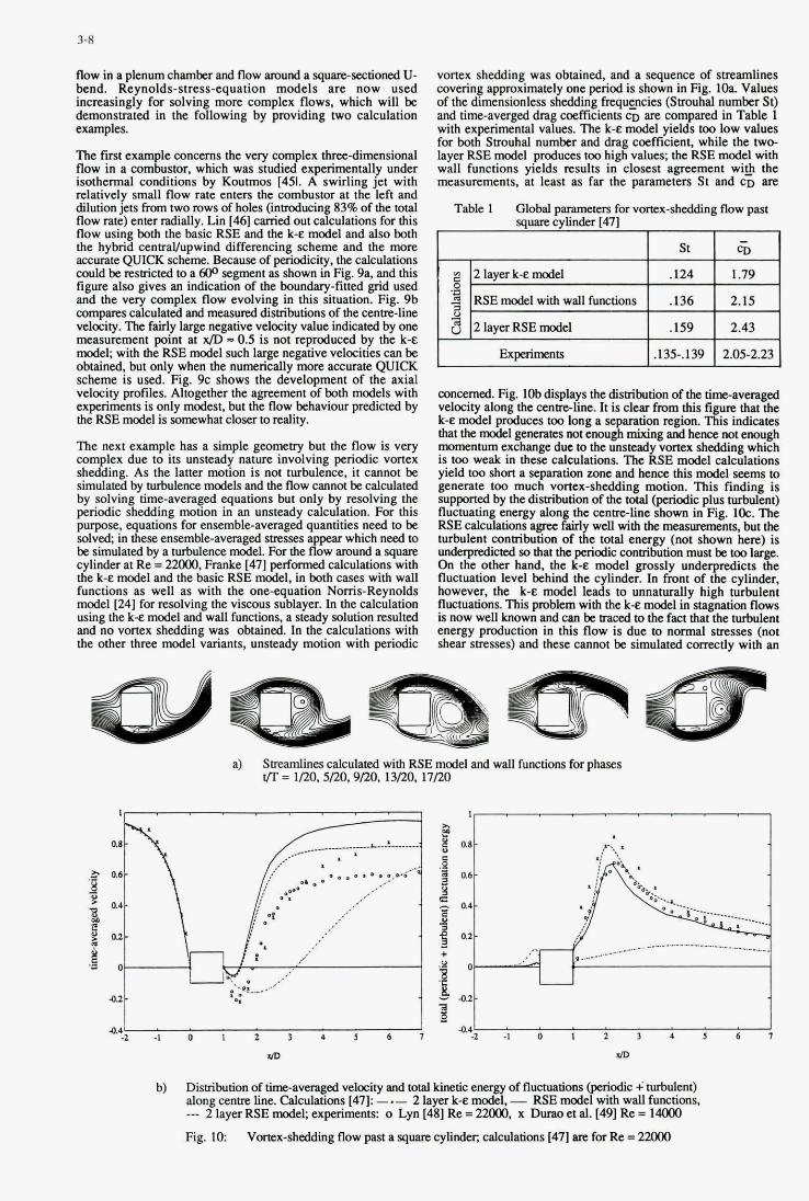
3-8

,159

flow in a plenum chamber and flow around a square-sectioned U- bend. Reynolds-stress-equation models are now used increasingly for solving more complex flows, which will be demonstrated in the following by providing two calculation examples.

The fmt example concerns the very complex three-dimensional flow in a combustor, which was studied experimentally under isothermal conditions by Koutmos [451. A swirling jet with relatively small flow rate enters the combustor at the left and dilution jets from two mws of holes ( inducing 83% of the total flow rate) enter radially. Lin [U] carried out calculations for this flow using both the basic RSE and the k-e model and also both the hybrid centralhpwind differencing scheme and the more accurate QUICK scheme. Because of periodicity, the calculations could be restricted to a 600 segment as shown in Fig. 9a, and this figure also gives an indication of the boundary-fitted grid used and the very complex flow evolving in this situation. Fig. 9b compares calculated and measured distributions of the centre-lire velocity. The fairly large negative velocity value indicated by one measurement point at JD = 0.5 is not reproduced by the k-e model; with the RSE model such large negative velocities can be obtained, but only when the numerically more accurate QUICK scheme is used. Fig. 9c shows the development of the axial velocity profiles. Altogether the apement of both models with expniments is only modest, but the flow behaviour predicted by the RSE model is somewhat closer to reality.

The next example has a simple geometry but the flow is very complex due to its unsteady nature involving periodic vortex shedding. As the laner motion is not turbulence. it cannot be simulated by turbulence models and the flow canna be calculated by solving time-averaged equations but only by resolving the periodic shedding motion in an unsteady calculation. For this purpose, equations for ensemble-averaged quantities need to be solved; in these ensemble-averaged stresses appear which necd to be simulated by a turbulence model. For the flow amund a square cylinder at Re = 22o00, Franke [47] performed calculations with the k-E model and the basic RSE model, in both cases with wall functions as well as with the onequation Noms-Reynolds model [24] for resolving the viscous sublayer. In the calculation using the k-e model and wall functions, a steady solution resulted and no vortex shedding was obtained. In the calculations with the other three model variants, unsteady motion with periodic

2.43

vomx shedding was obtained, and a sequence of suwnlines covering approximately one period is shown in Fig. 1Oa Values of the dimensionless shedding frequgncics (Strouhal numbcr St) and time-averged drag coefficients CD M c o m p d in Table 1 with experimental values. The k-e model yields too low values for both Stmuhal number and drag coefficient. while the t w ~ layer RSE model produces too high values; the RSE model with wall functions yields results in closest agreement with the measurements, at least as far the parameters St and CD are

Table 1 Global puramem for vortex-shedding flow past s a w cvlinder 1471

I S t I c o I

,124 I 1.79

I ,136 I 2.15 I R I I

I I.135-.139 I 2.05-2.23 1

concerned. Fig. lob displays the distribution of the dmc-averaged velocity along the ccna-line. It is clear from this figure that the k-e model produces too long a separation region. This indicates that the modcl generates wt enough mixing and hence not enough momentum exchange due IO the unstcady vortex shedding which i s 100 weak in these calculations. The RSE model calculations yield tw short a separation zone and hence this model seems to generate too much vortex-shedding motion. This finding is supponed by the distribution of the total (periodic plus turbulent) fluctuating energy along the ccnuelinc shown in Fig. IOc. The RSE calculations a p e fairly well with the m e a s m n t s . but the turbulent connibution of the total energy (not shown h m ) is un- ' so that the periodic contribution must k 100 large. On the other hand, the k-e model grossly underpredicts the fluctuation level behind the cylinder. In front of the cylinder. however, the k-E model leads to unnaturally high turbulent fluctuations. This pmblm with the k+ modcl in stagnation flows is now well known and cm be wced IO the fact that the turbulent energy production in this flow is due to normal stresses (not shear stresses) and these cannot be simulated comctly with an

a) Smeamlines calculated with RSE model and wall functions for phases r/r = 1/20,5/20,9/20,13/20,17/20

I

0.8

0.6

0.4

0 2

0

Q.2

4.4 4 -1 0 1 2 1 4 J 6 7

rlD

b) Disuibution of rim-averaged velocity and tnal Lincdc encrgy of fluctuations (periodic +turbulent) along cenm line. Calculations [47]: - .- 2 layer k< model, - RSE model with wall functions, -.- 2 layer RSE model; experiments: o Lyn 1481 Re = 22000. x Durao et al. [491 Re = 14wo

Fig. I O Voncx-shedding flow past a sqm cylindw, calculations (471 M for Re = 2ux)o

3-9

isotropic eddy-viscosity model, leading to excessive energy production. This problem does not arise when an RSE model is used. Overall, the RSE model leads to significantly improved predictions for vortex-shedding flows compared with the k-E model predictions because it can account for the anisotropy, history and transport effects which are important in these flows.

3.2

The model approximations that have entered the Reynolds-stress- equation (1 1) are fairly simple and do not satisfy certain theoretical constrains such as the realisability conditions due to Schumann [50], and they are also not compatible with the limiting two-dimensional behaviour of turbulence very near walls. Hence, considerable effort has gone into the development of improved models. Launder [42] has recently given a summary on these developments. Here only the main trends are briefly outlined.

Most important is the modelling of the pressure-strain term in the Reynolds-stress-equation, and hence most research effort has gone into this modelling, with the return to isotropy part $ij,1, and the rapid part $ijp being treated separately. Rotta's linear model for @j,l (given in equation 11) has the incorrect behaviour that $ij,l does not vanish in 2D turbulence as it should. This was remedied by i n d u c i n g more elaborate forms invoJing second and thii invariants of the anismpy tensor aij = (uiu'k - u36ij), see e.g. [42]. The isotropation of production model !or the rapid part $ij,2 given in equation (1 1) is also incompatible with 2D turbulence and shows an incorrect response in homogeneous shear layers to the variation of the ratio of production to dissipation of kinetic energy, &/E. Also for this part more elaborate models have been proposed [42, 521. involving quadratic and cubic terms. The more refined pressure-strain models were tested for relatively simple shear layers and were found superior to the model given in (1 l), but further testing of the somewhat complex models is certainly necessary before their general validity can be established

The assumption of local isotropy leading to the dissipation model in (1 1) is also not compatible with 2D turbulence. Hence. more elaborate relations for the dissipation rate of the individual stress components near walls were proposed, e.g. in [53]. More elaborate diffusion models have also been suggested in the literature, but in his review paper Launder [42] argues that in general their use is not really warranted, if only because the weaknesses of model predictions can seldom be traced to weaknesses of the diffusion model.

In the practical applications of standard RSE models such as the one given by eq. (1 1). the near-wall layer was not resolved and the damping of the normal fluctuations was accounted for by wall comaions to the pressure-strain model. The new, more complex pressure-strain models just discussed, which are consistent with the limiting 2D behaviour of turbulence at the wall, should help to simulate this damping effect. However, experience gained with these models so far [42] indicates that the use of these models alone seems not sufficient and that wall-correction terms, although reduced in magnitude, may still be necessary. In some near-wall RSE models which appeared in the literature, viscosity- dependent functions were introduced to simulate the damping effect, which appears to be mainly a pressure-reflection effect and is therefore not really affected by viscosity. However, some influence of viscosity may have to be brought in. Work on near- wall RSE modelling is in progress at various research institutions (e.g. at UMIST, Manchester, Arizona State University and Stanford University / NASA Ames). but it is fair to say that at present no thoroughly tested near-wall RSE model is available.

4 . CONCLUSIONS AND OUTLOOK

Simple turbulence models involving no differential equations or only an ordinary differential equation for the maximum shear stress will continue to be used in many practical calculations, especially for external aerodynamic flows, and they will be refined further. The k-e model will also continue for some time to play a key role in engineering calculations, and most of these calculations will be canid out with wall functions for many years to come. However, near-wall models will be used increasingly to replace the wall functions, at least in incompressible flows. A fairly large variety of different low-Reynolds-number k-E models

is now available, and the most recently developed ones show the c o m t near-wall behaviour as demonstrated by comparison with direct simulation data. However, the various model versions were tested mainly for simple boundary layers and their predictive ability, includm that for transition. has yet to be established for a

As the various damping functions in the low-Re k-e models were designed for use in boundary layers, the performance of these models in separated flows is not clear and has to be examined before the models can also be used with some confidence for these flows. For both boundary layers and 2D separated flows, encouraging results were obtained with a two-layer model, which employs the k-E model only in the outer part of the flow but resolves the near-wall region with a one-equation model. This model also needs further testing, in particular for three- dimensional situations. Here the question arises whether the computer resources available now and in the near future are sufficient for resolving the viscous sublayer with such a model also in 3D situations.

Reynolds-stressquation models will be used more and more for practical calculations in place of the k-E model, particularly for situations with complex strain fields and special effects on turbulence like due to streamline curvature, rotation etc.. Slowly, the more refined of the RSE models will come to be used, but considerable testing is still necessary before these models are ready for practical application; the same is true also for near-wall RSE models. The importance of direct numerical simulation data for testing the turbulence models and as basis for the development of new model assumptions will increase dramatically. However, as the Reynolds numbers possible in direct numerical simulations will go up only slowly, the resulting data will be restricted to fairly low Reynolds numbers and the main impact will remain in the area of near-wall modelling. For high Reynolds numbers, perhaps results h m large-eddy simulations can be exploited in a similar way, but these simulations are of course themselves dependent on model assumptions entering the subgrid-scale model, and sometimes they may rather be used directly as a predictive tool; in complex flow situations where the structure of turbulence is important or 3D timedependent calculations have to be carried out anyway, large-eddy or very-large-eddy simulations are likely to become the methods to be used in a few years' time [54]. However, in many application areas, conventional turbulence models will still be used and needed for many years to come.

5 . ACKNOWLEDGEMENTS

The work reported here was suppported partly by the Deutsche Forschungsgemeinschaft. The author is grateful to J. Cordes. R. Franke and D. Lyn for providing unpublished calculation results and to R. Zschemitz for the efficient typing of the manuscript.

wider range of B ows. especially for the newly proposed models.

6. 1.

2.

3.

4.

5 .

6.

7.

8.

REFERENCES Cebeci. T. and Smith, A.M.O.. "Analysis of Turbulent Boundary Layers". Academic Press. New York. 1974. Baldwin, W.S. and Lomax, H., "Thin-layer approximation and algebraic model for separated turbulent flows", AIAA Paper 87- 257. 1978. Johnson, D.A. and King, L.S., "A mathematically simple turbulence closure model for attached and separated turbulent boundary layers", AIAA J., 23.1985. pp. 1684-1692. Launder. B.E. and Spaldmg, D.B., "The numerical computation of turbulent flow", Comp. Meth. in Appl. Mech. and Eng., 3,

Iacovides, H. and Launder, B.E., 'The numerical simulation of flow and heat transfer in tubes in orthogonal-mode rotation", Proc. 6th Symp. on Turbulent Shear Rows, Toulouse, France, 1987. Viegas. J.R., Rubesin, M.W. and Hontman. C.C., "On the use of wall functions as boundary conditions for two-dimensional separated compksible flows", AIAA Paper 85-0180, 1985. Marvin, J.G.. "Progress and challenges in modeling turbulent aerodynamic flows". in Proc. Int. Symp. on Engineering Turbulence Modelling and Measurements. ed. W. Rodi, Elsevier Publishers, 1990. Patel. V.C.. Rodi. W. and Scheuerer. G.. "Turbulence models

1974, pp. 269-289.

for near-wail and iow-Reynolds-numb& flows: A review", AIAA J., 23, 1985, pp. 1308-1319.

3-10

9.

10.

11.

12.

13.

14.

15.

16.

17.

18.

19.

20.

21.

22.

23.

24.

25.

26.

27.

28. 29.

30.

31.

Myong. H.K. and Kasagi. N.. "A new approach to the improvement of k e turbulence model for wall-bounded shear flows", JSME Int. Journal, Series 11, 33, 1990, pp. 63-72. Nagano, Y. and Hishida, M., "Improved form of the k e model for wall turbulent shear flows", ASME J. Fluids Eng., 109,

Shih, T.H. and Mansour, N.N., "Modelling of near-wall turbulence". Proc. Int. Symp. on Engineering Turbulence Modelling and Measurements. ed. W. Rodi. Elsevier Publishers, 1990. Hanjalic. K.. "Practical predictions by two-equation and other fast methods", Proc. Zaric Memorial Int. Seminar on Wall Turbulence, Dubrovnik. Yugoslavia, Hemisphere Publishing Corp., 1988. Gibson. M.M. and Launder. B.E.. "Ground effects on pressure

1987, pp. 156-160.

fluctuations in the atmospheric boundary layer", J. Fluid Mech, 86, 1978. pp. 491-511. Launder, B.E.. "Low-Reynolds number turbulence near walls", UMIST Manchester, Dept. of Mech. Eng. Rept. TFD/86/4, 1986. Gilbert, N.. "Numerische Simulation der Transition von der laminaren in die turbulente KanalstxOmung". Report DFVLR - FB 88-55, DLR GUttingen. F.R. Germany, 1988. Rodi. W.. "The prediction of free turbulent boundary layers by use of a two-equation model of turbulence", Ph.D. Thesis, University of London. 1972. Chapman, D.R. and Kuhn, G.D., "The limiting behaviour of turbulence near a wall", J. Fluid Mech.. 170. 1986. pp. 265- 292. Lam, C.K.G. and Bremhorst, K.A., "Modified form of the k e model for predicting wall turbulence", ASME J. Fluids Eng., 103, 1981. pp. 456460. Kim, J., Moin, P. and Moser, R.. "Turbulence statistics in fully developed channel flow at low Reynolds number". J. Fluid Mech.. 177. 1987. pp. 123-166. Shih, T.H., "Turbulence modelling: Near-wall turbulence and effects of rotation on turbulence", CIR Annual Research Briefs, Centre for Turbulence Restwch, NASA Ames Research Centre and Stanford University, 1989. pp. 12-26. Chien, T.-Y.. "Predictions of channel and boundary-layer flows with a low-Reynolds-number turbulence model", AIAA J., 20,

Jones, W.P. and Launder, B.E., "The calculation of low- Reynolds-number phenomena with a twoequation model of turbulence", Int. J. Heat Mass Transfer, 16, 1973, pp. 1119- 1 130. Rodi, W. and Scheuerer, G., "Scrutinizing the k e model under adverse pressure gradient conditions". J. Fluids Eng.. 108,

Noms, L.H. and Reynolds, W.C., '"hrbulent channel flow with a moving wavy boundary", Rept. No. FM-10, Stanford University, Dept. Mech. Eng., 1975. Fujisawa. N., "Calculations of transitional boundary-layers with a refined low-Reynolds-number version of a k-e model of turbulence". Proc. Int. Symp. on Engineering Turbulence Modelling and Measurements, ed. W. Rodi, Elsevier Publishers, 1990. Fujisawa, N., Rodi. W. and Schllnung, B., "Calculation of transitional boundary layers with a two-layer model of turbulence", Proc. 3rd Int. Symp. on Transport Phenomena and Dynamics of Rotating Machinery, Honolulu, April 1990. Crawford, M.E. and Kays. M.W.. "STAN 5 - a program for numerical computation of two-dimensional intemal and external boundary-layer flows", NASA CR-2742,1976. Cordes. J.. private communication. 1988. Driver, D.M. and Seegmiller. H.L., "Features of a reattaching turbulent shear layer in divergent channel flow", AIAA J., 23.

Samuel, A.E. and Joubert, P.M., "A boundary layer developing in an increasingly adverse pressure gradient", J. Fluid Mech.,

Badri Narayanan, M.A. and Ramjee, V.. "On the criteria for reverse transition in a two-dimensional boundary layer flow". J. Fluid Mech., 35, 1969, pp. 225-241.

1982. pp.33-38.

1986. pp. 174-179.

1985. pp. 163-171.

66, 1974, pp. 481-505.

32.

33.

34.

35.

36.

37.

38.

39.

40.

41.

42.

43.

44.

45. 46.

47. 48. 49.

50.

51.

52.

53.

54.

BUhrle, P. "Numerische Bewhnung der abgelllsten Smmung Uber eine senkrechte ebene Platte mit einer zur AnstrOmung parallelen Trennplaae in der Symmetrieebene", Studiembeit an Institut fflr Hydromechanik, Universittit " h e , 1989. Jaroch, M., "Eine kritische Betrachhmg der Methode diskreter Wirbel als Modell fflr eine abge lh StxOmung mit geschlossener Abltlseblase auf der Basis experimenteller Erkenntnisse", Fortschrittsberichte VDI, Reihe 7,127,1987. Jaroch, M.P. and Femholz. H.H., "The three-dimensional character of a nominally two-dimensional se arated turbulent shear flow", J. Fluid Mech., 205, 1989, pp. 83-552. Rodi. W. and Scheuerer, G., "Calculation of laminar-turbulent boundary -layer transition on turbine blades", hoc. AGARD- PEP 65th Symp., Bergen, Norway, May 1985. Launder, B.E. and Sharma, B.I.. "Application of the energy- dissipation model of turbulence to the calculation of flow near a spinning disk", Letters in Heat and Mass Transfer, 1, 1974, pp.

Abu Ghannam, B.J.. "Boundary-layer transition in relation to turbomachinery blades". Ph.D. Thesis, University of Liverpool. Liverpool, U.K. 1979. Abu Ghannam, B.J. and Shaw, R., "Natural transition of boundary layers - the effects of hubulence. pressure gradient and flow history", J. Mech. Eng. Sci.. 22. 1980, pp. 213-228. Blair, M.F. and Werle, M.J., "The influence of free-stream tuhlence on the zero pressure gradient fully "lent boundary layer", UTRC Rept. R80-914388-12, 1980. Blair. M.F. and Werle. M.J., "Combined influence of free- turbulence and favourable pressure gradients on boundary-layer transition and heat transfer", UTRC Rept. 181-914388-17. 1981. Rodi. W., Liu. X. and Schllnung, B.. 'Transitional boundary layers with wake-induced unsteadiness". Proc. 4th Symp. on Numerical and Physical Aspects of Aerodynamic Flows, Long Beach, Califomia, January 1989. Launder, B.E., "Second-moment closure: present ... and future?", Int. J. Heat and Fluid Flow, 10, 1989. pp. 282-300. Leschziner. M.A.. "Second-moment closure for complex flows", Proc. Int. Forum on Mathematical Modelling of Processes in Energy Systems, Int. Centre for Heat and Mass Transfer, Sarajevo, March 1989. Launder, B.E., Reece, G.C. and Rodi, W.. "Progress in the development of a Reynolds-stress turbulence closure", J. Fluid Mech., 68. 1975. pp. 537-566. Koutmos. P., Ph.D. Thesis, University of London, 1985. Lin, C.A.. Ph.D. Thesis, Faculty of Technology. University of Manchester, 1989. Franke, R., private communication. 1990. Lyn. D., private communication, 1989. Durao, D.F.G., Heitor. M.V. and Pereira, J.C.F., "Measurements of turbulent and periodic flows around a square cross-sectioned cylinder'', Experiments in Fluids, 6, 1988, pp.

Schumann. U., "Realisability of Reynolds-stress turbulence models", Physics of Fluids, U), 1977, pp. 721-725. Lumley, J.L.. "Computational modelling of turbulent flows", in Advances in Applied Mechanics, 18, 1978, pp. 123-176. Academic Press, New Yo& Shih, P.H. and Lumley, JL., "Modelling of pressure-correlation terms in Reynolds stress and scalar flux equations", Rept. FDA- 85-3, Sibley School of Mech. and Aerospeace Eng., Comell University, 1985. Launder, B.E. and Reynolds, W.C.. "Asymptotic near-wall stress-distribution ram in turbulent flow". Physics of Fluids,

Reynolds, W.C., 'The potential and limitations of direct and largeeddy simulations", Position Paper at Conference "Whither Turbulence? or Turbulence at the Cross Road", Comell University, March 22-24. 1989, to be published by Springer in the Lecture Notes in physics Series.

131-138.

298-304.

26, 1983, pp. 1157-1158.

4- 1

TURBULENCE MODELS FOR NATURAL CONVECTION FLOWS ALONG A VERTICAL HEATED PLANE

by

D.D. Papailiou Laboratory of Applied Thermodynamics,

Dept. of Mechanical Engineering, University of Patras Kato Kostritsi, Patras 26.500, Greece

Introduction:

The present work has been prepared for presentation in the Technical Status Review on "Appraisal of the Suitability of Turbulence Models in Flow Calculations", organized by the Fluid Dynamics Panel of AGARD (Friedrichshafen, April 26, 1990). Its objective is to review the state of development of turbulent models currently employed in the computation of turbulent free convection flows along heated plane surfaces. In this context some experimental results recently obtained in the Laboratory of Applied Thermodynamics, University of Patras, are also compared with corresponding computations in which existing turbulence models were used.

Although free convection flows such as plumes, buoyant jets, thermals and those originated from heated surfaces, find wide application in various fields of science and technology including aeronautics, the understanding of turbulence transport processes in these cases is lagging behind as compared to other flows. This is generally due to the currently existing lack of sufficient knowledge regarding the effects of buoyancy on the turbulence structure of these flows and also its participation and role in the corresponding transport processes. The reasons causing this inadequacy of necessary information will be discussed in the following. As a consequence, in computing buoyancy induced flows, turbulent transport models are adopted from forced convection or ordinary flows, mostly in modified forms .

By reviewing the existing experimental evidence and computational methods currently in use for predicting the simple case of free convection turbulent flow along heated planes, it becomes possible to appreciate the difficulties presented in developing turbulence models for buoyancy driven flows. It also becomes possible to identify the sources of existing problems and limitations and finally, to suggest a course for future research activities in this particular area.

Most of the reported in the literature experimental and computationalwork on turbulent free convection, refers to Grashof or Rayleigh numbers corresponding to fully developed turbulent flow conditions. However, apart fromthe fact that both transitional and non-fully developed turbulence states are important on their own merits, their closer investigation might substantially help in improving free convection computational schemes. The study of these states of flow development could for instance result to the selection of more representative initial conditions and/or a more effective method for introducing turbulence action in the computations. More important, conditions prevailing in these states is known to affect the physical processes occurring in the following state of fully developed turbulence. The copined Yqperimental and computational effort in the region of Grashof numbers between 10 and 10 , presented in this work aims at exploring some of the above mentioned possibilities.

Turbulence Models for Free Convection Flow Along a Vertical Heated Plane:

The problem of turbulent free convection along a vertical heated wall, has been th subject of investigation for the past several decades. Numerous experiments have been reported in the literature (1-14), the majority of which has been limited to measurements of overall and local heat transfer coefficients and mean temperature distributions in the turbulent boundary layer. This is caused by existing inherent difficulties in measuring velocity in buoyant flows, especially near a heated wall where a combination of very low velocities and very steep temperature gradients dominate.

The lack of sufficient experimental information, which exist in abundance for most of the ordinary flows, appears to be mainly responsible for the inadequate understanding of buoyancy dominated free convection turbulent transport phenomena. As a consequence, this prevents the development of convincing theoretical arguments on which the modelling of turbulence transport terms will be based. At the present,almost all the theoretical efforts on the subject are based on analogies "borrowed" from forced convection flows.

The turbulence models which are presently employed in free convection boundary layer computations fall into three categories namely, algebraic (15, 16), standard U-E (17, 18) and low Reynolds number U-E (19-26). Algebraic models are using the concept of eddy diffusivity in forms either directly transferred from forced convection or modified for free convection. The latter two categories employ two equation U-E models describing turbulent kinetic energy and dissipation dynamics.

In the case of standard U-c modelling the use of wall functions is necessary to avoid the steep gradients prevailing near the wall and to provide boundary conditions for the U and E differential equations. Since no wall functions exist for turbulent free convection boundary layer,logarithmic wall functions, appropriate for forced convection boundary layer with small pressure gradients, are commonly used in computations (27).

In the case of low-Reynolds U--E models, the diminishing presence of turbulence near the wall is modelled by the introduction of a number of functions in the differential equations for U and E (27). It should be noticed that, here again, low-Reynolds number models used in free convection,with the exception of the model developed by To and Humphrey (26), have been originally developed for forced convection boundary layers.

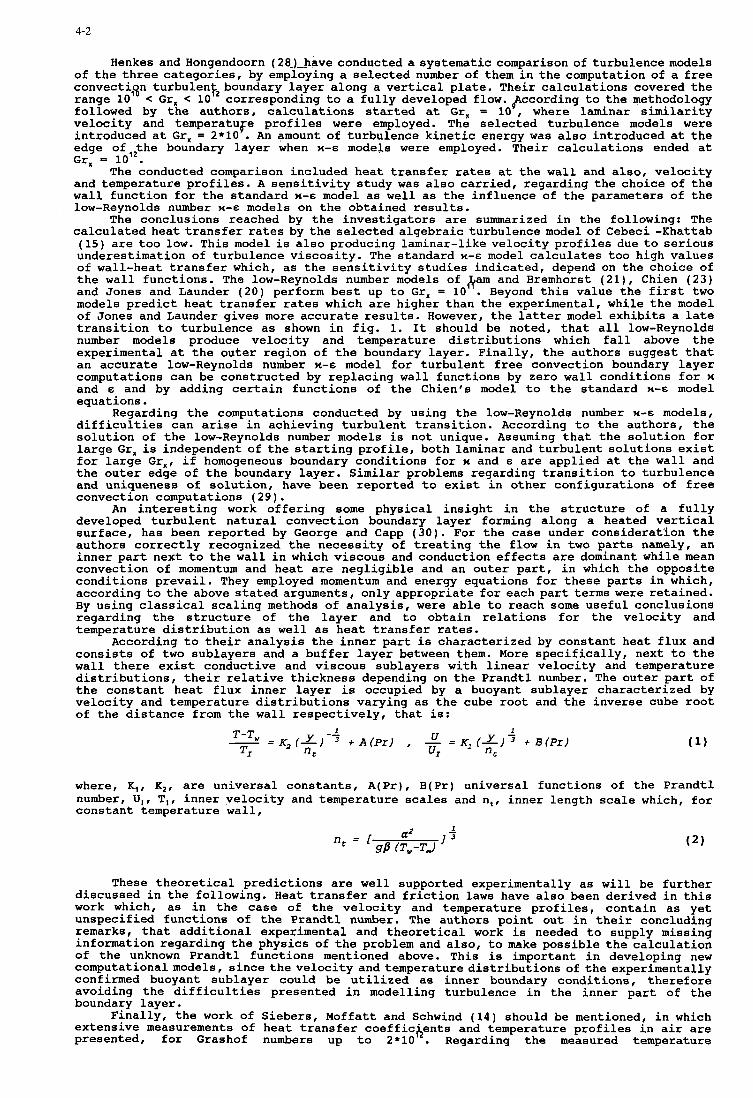
4-2

Henkes and Hongendoorn ( 28-)-have conducted a systematic comparison of turbulence models of the three categories, by employing a selected number of them in the computation of a free convectilqn turbulenf boundary layer along a vertical plate. Their calculations covered the range 10 < Gr, 10 ' corresponding to a fully developed flow. pccording to the methodology followed by the authors, calculations started at Gr, = 10, where laminar similarity velocity and temperatub-e profiles were employed. The selected turbulence models were introduced at Gr, = 2*10 . An amount of turbulence kinetic energy was also introduced at the edge oflzthe boundary layer when U-E models were employed. Their calculations ended at Gr, = 10 .

The conducted comparison included heat transfer rates at the wall and also, velocity and temperature profiles. A sensitivity study was also carried, regarding the choice of the wall function for the standard U-E model as well as the influence of the parameters of the low-Reynolds number H-E models on the obtained results.

The conclusions reached by the investigators are summarized in the following: The calculated heat transfer rates by the selected algebraic turbulence model of Cebeci -Khattab (15) are too low. This model is also producing laminar-like velocity profiles due to serious underestimation of turbulence viscosity. The standard H-E model calculates too high values of wall-heat transfer which, as the sensitivity studies indicated, depend on the choice of the wall functions. The low-Reynolds number models of &am and Bremhorst (21), Chien (23) and Jones and Launder (20) perform best up to Gr, = 10 . Beyond this value the first two models predict heat transfer rates which are higher than the experimental, while the model of Jones and Launder gives more accurate results. However, the latter model exhibits a late transition to turbulence as shown in fig. 1. It should be noted, that all low-Reynolds number models produce velocity and temperature distributions which fall above the experimental at the outer region of the boundary layer. Finally, the authors suggest that an accurate low-Reynolds number H-E model for turbulent free convection boundary layer computations can be constructed by replacing wall functions by zero wall conditions for H and E and by adding certain functions of the Chien's model to the standard H-E model equations.

Regarding the computations conducted by using the low-Reynolds number %-E models, difficulties can arise in achieving turbulent transition. According to the authors, the solution of the low-Reynolds number models is not unique. Assuming that the solution for large Gr, is independent of the starting profile, both laminar and turbulent solutions exist for large Gr,, if homogeneous boundary conditions for H and E are applied at the wall and the outer edge of the boundary layer. Similar problems regarding transition to turbulence and uniqueness of solution, have been reported to exist in other configurations of free convection computations (29).

An interesting work offering some physical insight in the structure of a fully developed turbulent natural convection boundary layer forming along a heated vertical surface, has been reported by George and Capp (30). For the case under consideration the authors correctly recognized the necessity of treating the flow in two parts namely, an inner part next to the wall in which viscous and conduction effects are dominant while mean convection of momentum and heat are negligible and an outer part, in which the opposite conditions prevail. They employed momentum and energy equations for these parts in which, according to the above stated arguments, only appropriate for each part terms were retained. By using classical scaling methods of analysis, were able to reach some useful conclusions regarding the structure of the layer and to obtain relations for the velocity and temperature distribution as well as heat transfer rates.

According to their analysis the inner part is characterized by constant heat flux and consists of two sublayers and a buffer layer between them. More specifically, next to the wall there exist conductive and viscous sublayers with linear velocity and temperature distributions, their relative thickness depending on the Prandtl number. The outer part of the constant heat flux inner layer is occupied by a buoyant sublayer characterized by velocity and temperature distributions varying as the cube root and the inverse cube root of the distance from the wall respectively, that is:

where, K,, K,, are universal constants, A(Pr), B(Pr) universal functions of the Prandtl number, U,, TI, inner .velocity and temperature scales and n,, inner length scale which, for constant temperature wall,

These theoretical predictions are well supported experimentally as will be further discussed in the following. Heat transfer and friction laws have also been derived in this work which, as in the case of the velocity and temperature profiles, contain as yet unspecified functions of the Prandtl number. The authors point out in their concluding remarks, that additional experimental and theoretical work is needed to supply missing information regarding the physics of the problem and also, to make possible the calculation of the unknown Prandtl functions mentioned above. This is important in developing new computationalmodels, since the velocity and temperature distributions of the experimentally confirmed buoyant sublayer could be utilized as inner boundary conditions, therefore avoiding the difficulties presented in modelling turbulence in the inner part of the boundary layer.

Finally, the work of Siebers, Moffatt and Schwind (14) should be mentioned, in which extensive measurements of heat transfer coefficAents and temperature profiles in air are presented, for Grashof numbers up to 2*10 . Regarding the measured temperature

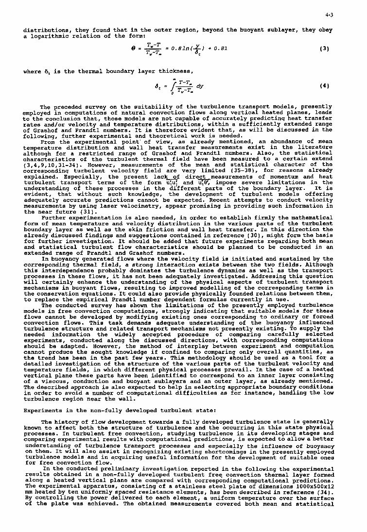
4-3

distributions, they found that in the outer region, beyond the buoyant sublayer, they obey a logarithmic relation of the form:

= 0 . 8 l n ( I ) + 0.81 (3) T -T

Tw-T" 6,

where 6, is the thermal boundary layer thickness, "

T-T, d, = /- dy T,-T,

The preceded survey on the suitability of the turbulence transport models, presently employed in computations of natural convection flows along vertical heated planes, leads to the conclusion that, those models are not capable of accurately predicting heat transfer rates and/or velocity and temperature distributions, within a sufficiently extended range of Grashof and Prandtl numbers. It is therefore evident that, as will be discussed in the following, further experimental and theoretical work is needed.

From the experimental point' of view, as already mentioned, an abundance of mean temperature distribution and wall heat transfer measurements exist in the literature although for a restricted range of Grashof and Prandtl numbers. Also, the statistical characteristics of the turbulent thermal field have been measured to a certain extend (3,4,9,10,31-34). However, measurements of the mean and statistical character of the correspondinq turbulent velocity field are very limited (35-38), for reasons already explained. Especially, the present l a c k 2 f direAmeasurements of momentum and heat turbulent transport terms of the form U;:; and u;V, impose severe limitations in the understanding of these processes in the different parts of the boundary layer. It is evident, that without such knowledge, the development of turbulent models offering adequately accurate predictions cannot be expected. Recent attempts to conduct velocity measurements by using laser velocimetry, appear promising in providing such information in the near future (31).

Further experimentation is also needed, in order to establish firmly the mathematical form of mean temperature and velocity distribution in the various parts of the turbulent boundary layer as well as the skin friction and wall heat transfer. In this direction the already discussed findings and suggestions contained in reference (30), might form the basis for further investigation. It should be added that future experiments regarding both mean and statistical turbulent flow characteristics should be planned to be conducted in an extended range of Prandtl and Grashof numbers.

In buoyancy generated flows where the velocity field is initiated and sustained by the corresponding thermal field, a strong interaction exists between the two fields. Although this interdependence probably dominates the turbulence dynamics as well as the transport processes in these flows, it has not been adequately investigated. Addressing this question will certainly enhance the understanding of the physical aspects of turbulent transport mechanisms in buoyant flows, resulting to improved modelling of the corresponding terms in the conservation equations. It could also provide physically founded relations between them, to replace the empirical Prandtl number dependent formulas currently in use.

The conducted survey has shown the limitations of the presently employed turbulence models in free convection computations, strongly indicating that suitable models €or these flows cannot be developed by modifying existing ones corresponding to ordinary or forced convection flows. This task demands adequate understanding of the buoyancy influenced turbulence structure and related transport mechanisms not presently existing. TO supply the needed information the widely accepted procedure of comparing carefully selected experiments, conducted along the discussed directions, with corresponding computations should be adapted. However, the method of interplay between experiment and computation cannot produce the sought knowledge if confined to comparing only overall quantities, as the trend has been in the past few years. This methodology should be used as a tool for a detailed investigation of the structure of the various parts of the turbulent velocity and temperature fields, in which different physical processes prevail. In the case of a heated vertical plane these parts have been identified to correspond to an inner layer consisting of a viscous, conduction and buoyant sublayers and an outer layer, as already mentioned. The described approach is also expected to help in selecting appropriate boundary conditions in order to avoid a number of computational difficulties as for instance, handling the low turbulence region near the wall.

Experiments in the non-fully developed turbulent state:

The history of flow development towards a fully developed turbulence state is generally known to affect both the structure of turbulence and the occurring in this state physical processes. In turbulent free convection, studying turbulence in its developing stages and comparing experimental results with computational predictions, is expected to allow a better understanding of turbulence transport processes and especially the influence of buoyancy on them. It will also assist in recognizing existing shortcomings in the presently employed turbulence models and in acquiring useful information for the development of suitable ones for free convection flow.

In the conducted preliminary investigation reported in the following the experimental results obtained in a non-fully developed turbulent free convection thermal layer formed along a heated vertical plane are compared with corresponding computational predictions. The experimental apparatus, consisting of a stainless steel plate of dimensions 1000x500~12 nun heated by ten uniformly spaced resistance elements, has been described in reference (34). By controlling the power delivered to each element, a uniform temperature over the surface of the plate was achieved. The obtained measurements covered both mean and statistical

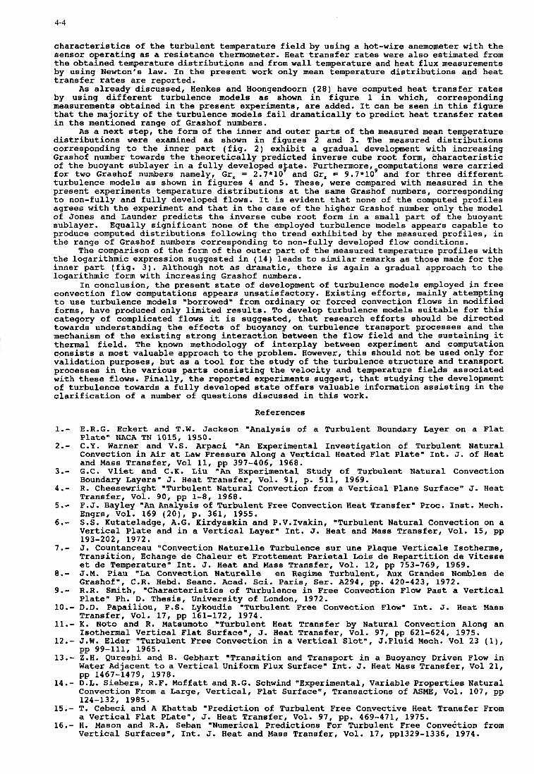
4-4

characteristics of the turbulent temperature field by using a hot-wire anemometer with the sensor operating as a resistance thermometer. Heat transfer rates were also estimated from the obtained temperature distributions and from wall temperature and heat flux measurements by using Newton's law. In the present work only mean temperature distributions and heat transfer rates are reported.

As already discussed, Henkes and Hoongendoorn (28) have computed heat transfer rates by using different turbulence models as shown in figure 1 in which, corresponding measurements obtained in the present experiments, are added. It can be seen in this figure that the majority of the turbulence models fail dramatically to predict heat transfer rates in the mentioned range of Grashof numbers.

As a next step, the form of the inner and outer parts of the measured mean temperature distributions were examined as shown in figures 2 and 3. The measured distributions corresponding to the inner part (fig. 2) exhibit a gradual development with increasing Grashof number towards the theoretically predicted inverse cube root form, characteristic of the buoyant sublayer in a fully developed sFate. Furthermore,,computations were carried for two Grashof numbers namely, Gr, = 2.7*10 and Gr, = 9.7*10 and for three different turbulence models as shown in figures 4 and 5. These, were compared with measured in the present experiments temperature distributions at the same Grashof numbers, corresponding to non-fully and fully developed flows. It is evident that none of the computed profiles agrees with the experiment and that in the case of the higher Grashof number only the model of Jones and Launder predicts the inverse cube root form in a small part of the buoyant sublayer. Equally significant none of the employed turbulence models appears capable to produce computed distributions following the trend exhibited by the measured profiles, in the range of Grashof numbers corresponding to non-fully developed flow conditions.

The comparison of the form of the outer part of the measured temperature profiles with the logarithmic expression suggested in (14) leads to similar remarks as those made for the inner part (fig. 3). Although not as dramatic, there is again a gradual approach to the logarithmic form with increasing Grashof numbers.

In conclusion, the present state of development of turbulence models employed in free convection flow computations appears unsatisfactory. Existing efforts, mainly attempting to use turbulence models "borrowed" from ordinary or forced convection flows in modified forms, have produced only limited results. To develop turbulence models suitable for this category of complicated flows it is suggested, that research efforts should be directed towards understanding the effects of buoyancy on turbulence transport processes and the mechanism of the existing strong interaction between the flow field and the sustaining it thermal field. The known methodology of interplay between experiment and computation consists a most valuable approach to the problem. However, this should not be used only for validation purposes, but as a tool for the study of the turbulence structure and transport processes in the various parts consisting the velocity and temperature fields associated with these flows. Finally, the reported experiments suggest, that studying the development of turbulence towards a fully developed state offers valuable information assisting in the clarification of a number of questions discussed in this work.

References

1.- E.R.G. Eckert and T.W. Jackson "Analysis of a Turbulent Boundary Layer on a Flat Plate" NACA TN 1015, 1950.

2.- C.Y. Warner and V.S. Arpaci "An Experimental Investigation of Turbulent Natural Convection in Air at Law Pressure Along a Vertical Heated Flat Plate" Int. J. of Heat and Mass Transfer, Vol 11, pp 397-406, 1968.

3.- G.C. Vliet and C.K. Liu "An Experimental Study of Turbulent Natural Convection Boundary Layers" J. Heat Transfer, Vol. 91, p. 511, 1969.

4.- R. Cheesewright "Turbulent Natural Convection from a Vertical Plane Surface" J. Heat Transfer, Vol. 90, pp 1-8, 1968.

5.- F.J. Bayley "An Analysis of Turbulent Free Convection Heat Transfer" Proc. Inst. Mech. Engrs, Vol. 169 (20), p. 361, 1955.

6.- S.S. Kutateladge, A.G. Kirdyaskin and P.V.Ivakin, "Turbulent Natural Convection on a Vertical Plate and in a Vertical Layer" Int. J. Heat and Mass Transfer, Vol. 15, pp

7.- J. Countanceau "Convection Naturelle Turbulence sur une Plaque Verticale Isotherme, Transition, Echange de Chaleur et Frottement Parietal Lois de Repartition de Vitesse et de Temperature" Int. J. Heat and Mass Transfer, Vol. 12, pp 753-769, 1969.

8.- J.M. Piau "La Convection Naturelle en Regime Turbulent, Aux Grandes Nombles de Grashof", C.R. Hebd. Seanc. Acad. Sci. Paris, Ser. A294, pp: 420-423, 1972.

9.- R.R. Smith, "Characteristics of Turbulence in Free Convection Flow Past a Vertical Plate" Ph. D. Thesis, University of London, 1972.

10.- D.D. Papailiou, P.S. Lykoudis "Turbulent Free Convection Flow" Int. J. Heat Mass Transfer, Vol. 17, pp 161-172, 1974.

11.- K. Noto and R. Matsumoto "Turbulent Heat Transfer by Natural Convection Along an Isothermal Vertical Flat Surface", J. Heat Transfer, Vol. 97, pp 621-624, 1975.

12.- J.W. Elder "Turbulent Free Convection in a Vertical Slot", J.Fluid Mech. Vol 23 (l),

13.- Z.H. Qureshi and B. Gebhart "Transition and Transport in a Buoyancy Driven Flow in Water Adjacent to a Vertical Uniform Flux Surface" Int. J. Heat Mass Transfer, Vol 21, pp 1467-1479, 1978.

14.- D.L. Siebers, R.F. Moffatt and R.G. Schwind "Experimental, Variable Properties Natural Convection From a Large, Vertical, Flat Surface", Transactions of ASME, Vol. 107, pp

15.- T. Cebeci and A Khattab "Prediction of Turbulent Free Convective Heat Transfer From a Vertical Flat PLate", J. Heat Transfer, Vol. 97, pp. 469-471, 1975.

16.- H. Mason and R.A. Seban "Numerical Predictions For Turbulent Free Convection from Vertical Surfaces", Int. J. Heat and Mass Transfer, Vol. 17, pp1329-1336, 1974.

193-202, 1972.

pp 99-111, 1965.

124-132, 1985.

4-5

17.- O.A. Plumb and L.A. Kennedy 'Application of a x-6 Turbulence Model to Natural Convection from a Vertical Isothermal Surface', J. Heat Transfer, vol. 99, pp 79-85, 1977.

18.- S.J. Lin and S.W. Churchill * Turbulent Free Convection from a Vertical, Isothermal Plate", Numer. Heat Transfer, Vol 1, pp 129-145, 1978.

19.- S. Hassid and M. Poreh 'A Turbulent Energy Dissipation Model for Flows with Drag Reduction", J. Fluids Eng., Vol 100, pp 107-112, 1978.

20.- W.P. Jones and B.E. Launder "The Prediction of Laminarization with a Two-Equation Model of Turbulence", Int. J. Heat and Mass Transfer, Vol. 15, pp. 301-314, 1972.

21.- C.K.G. Lam and K. Bremhorst .A Modified form of the xi6 Model for Predicting Wall Turbulence', J. Fluids Engng, Vol 103, pp 456-460, 1981.

22.- K.Y. Chien, "Predictions of Channel and Boundary Layer Flows with a Low-Reynolds number Two-Equation Model of Turbulence" AIM-80-0134, 1980.

23.- K.Y. Chien, " Predictions of Channel and Boundary Layer Flows with a Low-Reynolds number Turbulence Model., A I M J., Vol.20, pp 33-38, 1982.

24.- W.C. Reynolds, "Computation of Turbulent Plows', Ann. Rev. Fluid Mech., Vo1.8, pp 83-208, 1976.

25.- G.H. Hoffman, 'Improved Form of the Low Reynolds Number x-6 Turbulence model', Physics of Fluids, Vo1.18, pp 309-312, 1915.

26.- W.M. To and J.A.C. Humphrey, "Numerical Simulation of Buyoant Turbulent Flow-1.Free Convection Along a Heated Vertical Flat Plate', Int. J. Heat and Has8 Transfer, Vol. 29. DD 513-592. 1986. . ..

27.- V.C. Patel, W. Rodi and G. Scheuerer "Turbulence Models for Near-Wall and Low-Reynolds number Flows a Review', A I M J., Vol. 23, pp 1308-1319, 1985.

28.- R.A.W.M. Henkes and C.J. Hoogendoorn "Comparison of Turbulence Models for the Natural Convection Boundary Layer Along a Heated Vertical Plate', Int. J. Heat and Mass Transfer, Vo1.32, pp. 151-169, 1989.

29.- H. O z o e , A. Mouri. M. Ohmuro. S.W. Churchill and N. Lior "Numerical CalculatiOnS of

30.-

31.-

32.-

33.-

34.-

35.-

36.-

37.-

38. -

Laminar. and Turbuient Naturai Convection in water in Rectangular Channels Heated and Cooled Isothermally on the Oposing Vertical Walls" Int. J. Heat and Mass Transfer , V01.28, pp. 125-138, 1985. W.K. George and S.P. Capp "A theory for natural convection turbulent Boundary Layers Next to Heated Vertical rrurfaces', Int. J. Beat and Mass Transfer,Vol.ZZ, pp. 813-826, 1969. M. Miyamoto, 8. Kajino, J. Karima and I. Takanami "Development of Turbulence Characteristics in a Vertical Free Convection Boundary Layer', Proc. 7th Int. Heat Transfer Conf., Vol.2, pp. 323-328, 1982. D.D. Papailiou 'Statistical characteristics of a Turbulent Free-Convection Flow in the Absence and Presence of a Magnetic Field', Int. J. Heat and Mass Transfer, Vol. 23, pp. 889-895, 1980. K. Kitamura, M. Koike, I. Fukuoka and T.S. Saito "Large Eddy Structure and Heat Transfer of Turbulent Natural Convection Alona a Vertical Flat Plate .. Int. J. of Heat and Mas8 Transfer, Vol. 28, pp 837-850. i985. T.J. Tsirikoglou and D.D. Papailiou "The Structure of the Turbulent Temperature Field Above Heated Planes". Published in the - Advances in Turbulence *, Editors: G. Comte-Bellot and J. Mathieu, Springer-Verlag, pp 300-309, 1987. R. Cheesewrite and E. Ierokipiotis "Velocity Measurements in a Natural Convection Boundary Layer., Queen Mary Colege, Faculty of Engineering Research, Report EP 5022, 1981. R.Cheesewrite and E. Ierokipiotie 'Velocity measurements in a Turbulent Natural Convection Boundary Layer" Proc. 7th Int. Heat Transfer Conf., Vol. 2, pp 305-309, Munich, F.R.G., 1982. C.J. Hoogendoorn and H. Euser, 'Velocity Profiles in the Turbulent Free Convection Boundary Layer', Proc. 6th Int. Heat Transfer Conf., Vol. 2, pp 193-198, 1978. M. Hishida, Y. Nagamo, T. Tsuji and I. Kaneko, 'Turbulent Boundary Layer of Natural Convection Along a Vertical Flat Plate", Trans. Japan Soc. Mech. Engrs, Vol. 47, pp 1260-1268, 1981.

4-6

0.0 ls0I

Fig. 1. Computed and measured wall heat t ransfer f o r a i r .

Henkes and Hoogendoorn r e f . (28)

+

Linear

+ + +

0.4

+++++ Grx=3.71x10’0 Smith * * * * * Gr.=0.97 0.2 00000 Gr.=0.84

AAAAA Gr.=0.62 DDDDD Gr.=0.54 00000 Grx=0.27

Present Experiments

0.0

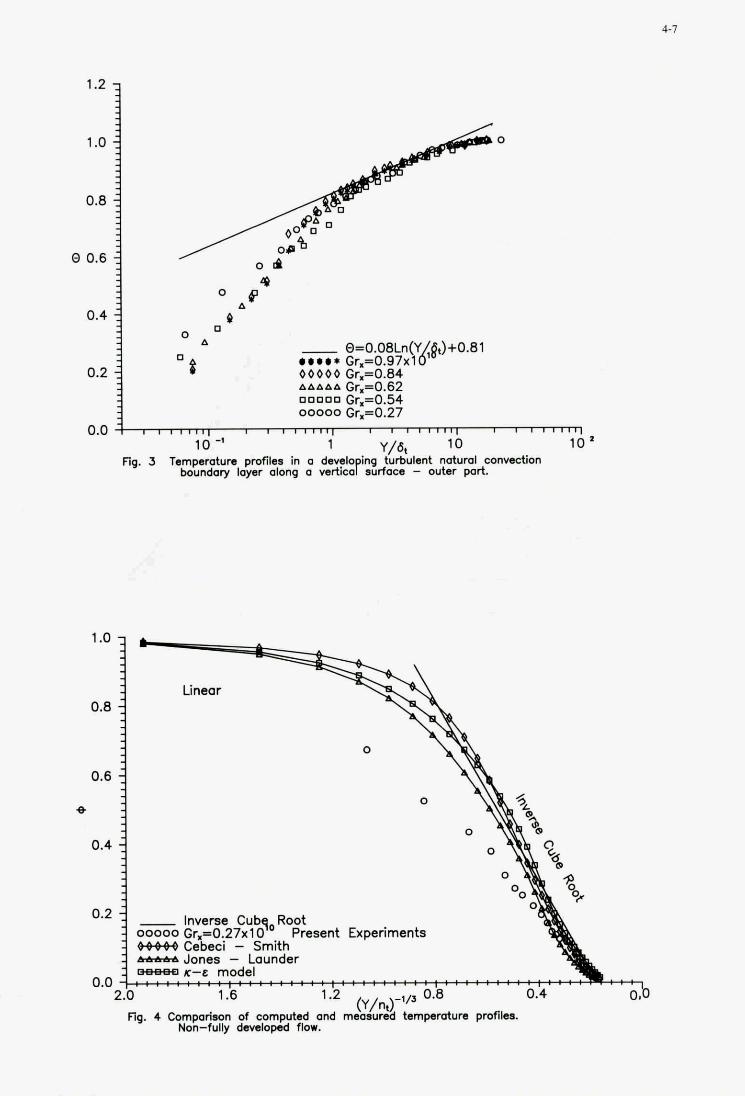
0.4 1

4-7

4 O B A

4 - 0

__ Q=0.08Ln\Ydft)+0.81 * Grx=0.97x 00000 Grx=0.84 A A A A A cr.=n.e3

0.2 _."

o n o ~ ~ Gr.=0.54 ooooo Grx=0.27

1 1 U 10 10 * 10 4 1 Y/8,

Fig. 3 Temperature profiles in a davelo ing turbulent natural convection boundary layer along a VerticoPsurface - outer port.

1 .o

0.8

0.6

0

0.4

- inverse Cub5,Root ooooo GrX=0.27x1 0 Present Experiments

0.2

0.0

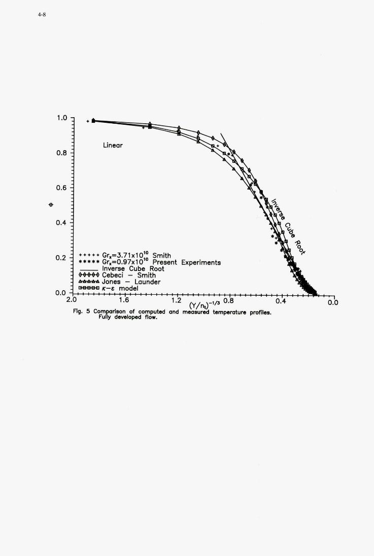
5-1

TURBULENT FLOW MODELLING IN SPAIN. OVERVIEW AND DEVELOPMENTS.

C. Dopazo, R. Aliod and L. Valiiio Fluid Mechanics Group, School of Engineering

University of Zaragoza M. Luna, 3,50015 Zaragoza

Spain

ABSTRACT

A brief overview of ongoing flow modelling activities in Spain in the fields of turbulent boundary layers, two- phase flows and turbulent reactive flows is presented.

Turbulent shear flows laden with small solid particles and the turbulent isothermal mixing of two chemical species undergoing a second order irreversible chemical reaction are discussed in more detail. An eulerian approach is followed in the former, employing a phase indicator function conditioning technique for the continuous phase and a Bolmann type velocity distribution function for the dispersed phase. The latter is treated via a probability density function (pdf) formalism where the joint statistics of concentrations and concentration-gradients is investigated. Predictions are compared with available experimental results in both cases.

Some concluding remarks on the specific needs on modelling or turbulent two-phase and reacting flows are listed.

1. INTRODUCTION

As in most fields of scientific research, the ultimate goal in the investigation of turbulent flows is to develop a quantitative tractable predictive theory. This objective is hampered by the existence of a wide spectrum of length and time scales, ranging from the characteristic sizes and frequencies of the large turbulent structures to the Kolmogorov length and time microscales. This prevents direct numerical simulation (DNS) of turbulent flows in most cases of practical interest. DNSW 161 31.36 of some idealized and limit cases can provide useful information on the asymptotic behavior of turbulent fields.

Existing computers set a limit on the length and time scales that can be numerically resolved. Large eddy simulation (LES) methodology21 filters the contribution to a fluctuating variable coming from large structures averaging the effects of small scales below a given threshold. The latter introduce unknown terms in the resulting equations. Models or closure hypothesis must be proposed in order to proceed further to the numerical simulation. In some instances, dumping the small scale contributions into a collective pool may yield good results. This can be the case of the turbulence modelling where most energy production and energy transfer processes are dominated by large/intermediate size eddies, while the overall small-scale action upon the flow can be simulated and quantified as a diffusive-like irreversible mechanism. However, if a process is tied to the small fluctuating scales the closure difficulties might render LES strategies useless. This is the case of chemically reacting turbulent flows.

Reynolds averaging techniques consider the contribution to a fluctuating variable coming from the whole spectrum of length and/or time scaleszs. The closure problem can be more severe and difficult to solve than the equivalent one in LES for the velocity field or of the same order to complexity for a reactive scalar in a turbulent flow. Moment and probability density function (pdf) equations have been obtained after Reynolds- averaging the corresponding local-instantaneous consevation equations. Most modelling activity has revolved around moment-equations'8J9. Pdf transport equations condense the information equivalent to an infinite hierarchy of moment equations9.10.25. It has been shown that the pdf formalism is the natural one for turbulent reactive flows10 and that pdf models can be proposed based on second order closure models29.

An overview of ongoing activities on turbulent flow modelling in Spain is presented in Section 2. Modelling work on turbulent boundary layers, two-phase flows and turbulent reactive flows is briefly described. More details with emphasis on closure models are provided in Section 3 for two selected cases: Turbulent shear flows laden with small solid particles and turbulent isothermal mixing of an acid and a base undergoing a second order irreversible chemical reaction; these cases exemplify two areas in which significant modelling efforts are required. In the former even the basic equations and methodologies to be used as a starting point are being questioned. The latter is adequate to illustrate the difference between what seems to be the natural pdf approach and what most moment modellers in the field are doing. Section 4 contains some concluding remarks on the two selected cases.

2. OVERVIEW

The following ongoing turbulent flow modelling activities in Spain have been brought to the attention of the authors:

2.1 Turbulent Boundary Lavers

2.1.1 Asvmptotic Expansion Techniaues7.26

Turbulence modelling is being conducted via the asymptotic techniques originated within the framework of "periodic homogeneization theory". The flow variables are asymptotically expanded and the model can, thus, be formally justified. The averaged partial differential equations have a structure analogous to that of the compressible Navier-Stokes equations.

The starting point is the so called MPP turbulence models 20, valid for incompressible flows of ideal or weakly viscous fluids. These models have been generalised in a first attempt7 to inviscid compressible

5-2

isentropic flows. No closure hypothesis are required at this level. The Reynolds stress tensor is obtained from the solution of a non-linear differential equation. The gradient of the inverse lagrangian coordinate associated to the mean velocity field, the average turbulent kinetic energy and the average helicity appear as parameters in that equation. The unclosed terms can then be tabulated and it is to be expected that the corresponding table has a universal character26. These models do not take into account the flow behavior near solid walls. On the other hand, mechanisms for turbulence generation are not considered and models are typically non-stationary.

As a first step, a reformulation of asymptotic models for moderately high Reynolds number and moderate Mach number compressible isentropic flows has been achieved. Non-standard boundary conditions adding new non-linearities to the problem and based on the well known logarithmic law of the wall have been introduced to take into account the existence of boundary 1ayers.The methodology followed to numerically solve the problem is described in detail in Reference 26 where a large number of numerical results are presented.

In a second step, new models describing the turbulent motion of the fluid over the whole domain, including the regions near solid walls, have been formulated. The flow domain is decomposed into a turbulent boundary layer and an inviscid outer zone. Small parameters are introduced and asymptotic expansions for the flow variables are hypothesized for the different zones. Formal manipulation of the equations, identifying the coefficients of the various powers of the small parameters, lead to averaged variable equations for the inner and outer zones. The original initial and boundary conditions are supplemented with those obtained from "matching" the inner and outer variables. The use of these models allows, among other things, to rigorously justify, from the asymptotic point of view, the laws of the wall.

The numerical solution rest upon semi-implicit time discretization schemes and finite element type approximation for the space variables. A least square type formulation is utilized followed by an algorithm of the Buckley-Le Nir conjugate gradients. Finally, the numerical problem is reduced to the solution of a "cascade" of linear problems, some of them analogous in nature to the Stokes problem, which can be solved using, for example, the Glowinski-Pironneau method, and others of the Poisson type.

These techniques are being developed within the framework of the HERMES Project of the European Space Agency (ESA) in order to predict the thermal behavior of this space aircraft during its reentry into the earths's atmosphere. 2.1.2 Algebraic Model of Turbulence1

The two-dimensional (2D) compressible laminar Navier-Stokes equations are considered in a nondimensional form,

where the flux vectors F and G can be expressed as F = F' + FV , G = GI + GV.The superscripts I and V denote inviscid and viscous contributions, respectively, and

0 Fv= 11 - - T ' ~ ~ ~ ~ 5 1

Re P a r P r X - U TIl1 - v 2' + -

Here Re and P, denote the Reynolds and Prandtl numbers respectively, U and v the two components of the velocity vector and p, e, p, h and T are the dimensionless density, specific total energy, pressure, specific total enthalpy and temperature of the fluid. The Sutherland relation is used to take into account the dependence of the molecular viscosity coefficient, p, on temperature and Mach number. The non-dimensional components of the stress tensor, 2 1 1 , 2 1 2 and 222 are assumed to follow the Navier-Poisson relation for laminar flows. The equation of state complete the problem specification.

For turbulent flows p is replaced by "pi + pt". pi is the laminar viscosity. For the "eddy viscosity coefficient", pt, the Baldwin-Lomax algebraic model4 is used. The variables in Equ. (2) stand then for average values. Cebeci's modifications avoid the calculation of the boundary layer edge.

In this two-layer model the turbulent viscosity is given by 9

Pti for Y 5 Yco

(3)

where pti and pto stand for inner and outer values of pt, y is the normal distance to the wall and yw is the cross- over value, the minimum y for which the inner and outer values of pt are equal.

Van-Driest formulation is followed for pti ,

where Ci is a constant, and

l=k y [I - exp (- y+/A+)]

w is the mean vorticity module given by,

5-3

I m L -=J($-s,

and y+ = Y ~ d n , with U* being the friction velocity and v the kinematic viscosity. Clauser formulation is used to express pto,

pto = K %p Fw Fk(Y) (7 )

K is Clauser constant, C, is an additional constant and

Fmax is the maximum value of

F(y) = y [ 1 - exp (- y+/A+)I (9)

and ymax is the value of y at which F(y) = Fmm. FK(Y) is the Klebanoff intermittency factor,

udif is the difference between the maximum and minimum values of the velocity for a profile. The standard values are assigned to the constants.

The solution is obtained by advancing the unsteady nondimensional form of the equations to steady state by means of a hybrid timestepping scheme. The convergence is accelerated by the use of local timestepping and the incorporation of implicit residual averaging. Spatial discretization is accomplished by means of a Galerkin finite element method assuming a general unstructured grid of linear three-noded triangular elements. In the code, this is achieved by the equivalent process of computing the element contributions from a loop over all the element sides in the mesh. To ensure complete vectorisation of this procedure, the element sides are automatically coloured by the mesh generatorl. The resulting scheme is stabilised by the application of an artificial dissipation operator which is formed as a blended combination of second and fourth differences.

2.2 Two-Phase Flows

2.2.1 DisDersed Phase as a Continuum15

A monodispersed cloud of rigid spheres syspended in an incompressible isothermal viscous gas is considered. No mass transfer between the phases is included. The dynamic behavior of the particles is characterized by continuous velocity, pressure and concentration fields. For a distribution of particle sizes, as many velocity, pressure and concentration fields are required as the number of size families to be treated.

The particle/particle and particle/fluid interactions are simulated by the introduction of a "pressure" and a "viscosity" of the particle cloud and an inter-phase force taking into account the momentum transfer between the phases.

Should the particle cloud viscosity be ignored no macroscopic mechanism exists to set a limit to strong gradients. A discrete system of particles has been analysed in order to find a strong-gradients limiting mechanism for the continuum model. The inviscid flow around an ensemble of spherical particles has been investigated. None of the microscopic terms can prevent the development of strong gradients in the particle concentration. The consideration of the cloud viscosity seems thus to be neccesary in order to describe small wavelengths.

On the other hand, the functional dependence of the particle cloud pressure is important and has significant macroscopic consequences upon the flow development 15.

The specification of the particle cloud viscosity and pressure are therefore open topics. The viscosity data measured by SchiirgeP for glass spherical particles of various diameters have been analysed. The viscosity increases considerably when the fluidised bed concentration approaches the maximum packing concentration; on the other hand, it has been observed that a dimensionless viscosity can be obtained by scaling the experimental data with the particle density, the fluidization velocity and a characteristic length which is a function of the particle diameter and Reynolds number. A universal curve of the dimensionless viscosity as a function of the volume concentration can then be plotted. More experiments are however necessary in order to ascertain the suspension rheological behavior.

At moderately high loads the particles interact mainly with the surrounding fluid and the stresses of the cloud are mostly due to particle/fluid interactions. On the other hand, for high cloud concentrations the frequency of collisions between particles increases and the pressure of the particle cloud should substantially grow, preventing the cloud from attaining concentrations above that of maximum packing. Neither experimental data nor theoretical developments exist to model the cloud pressure at high concentration. However, the correct modelling of the pressure is essential, as this is an important mechanism limiting the maximum value of particle concentration.

2.2.2 Eulerian Formulation of Average Eauation~23

In the theoretical derivation of two-phase flow equations, extensive use is made of conditioned averaging techniques8.11. Spatial, temporal, or ensemble average and double/mixed average operators are frequently found in the literature . Two consecutive averages are also encountered in turbulent two-phase flow modeling. Nevertheless the existing formalisms are not quite satisfactory, specially in dealing with turbulent flows. Volume or time averaging produce filtering of small-scale turbulent structures or large fluctuating frequencies. To avoid that filtering effect, dispersed elements must be much smaller than Kolmogorov scales and the number of elements inside the probe volume large enough to get stable values. Those situations rarely occur in practice and are impossible to satisfy in dilute flows. Ensemble averages

5-4

avoid these problems but the interaction terms have no straightforward meaning and must be interpreted by comparison with other averages. Applying two consecutive averages lead to equations with a large number of terms with no direct physical meaning and include high order fluctuation correlations, creating some serious closure problems.

Following the usual conditioning technique based on a phase-indicator function3 and properly defining a joint probability density function to describe the dispersed phase dynamics, some of the ideas pointed out by Herczynski and Pienkowskal4 are generalized. Theorems and associated properties are given allowing a general, rigorous and systematic treatment of the continuous phase of a dispersed two-phase flow system. The conditioned mean value of any variable derivative can be expressed as the derivative of the variable conditioned mean value, plus an extra interface source term, which will introduce in the equations information about the action of the second phase.The formalism employed, shares some features in common with those previously developed. The difficulties mentioned above are however overcome. Using those results conditioned average continuity, momentum turbulent kinetic energy and turbulence dissipation rate equations for the continuous phase can be obtained. The main characteristics of these equations are:

- General applicability. In principle no restrictions are placed on the sizes of dispersed elements or their concentrations.

- Continuous phase variables appear statistically averaged. Therefore no spatial or temporal filtering is performed. - Continuous phase equations are obtained in a single- step averaging operation.

- Continuous phase equations are formally indentical to those in classical turbulent single-phase flows, with similar terms and the same order of fluctuation correlations.

An axisymmetric turbulent jet configuration has been chosen to validate the model for both single phase and two-phase flows. A classical finite volume four-node formula space?marching fully-implicit scheme has been used. Validation has been conducted by comparing the model predictions with available experimental data12.B. Preliminary predictions indicate a reasonably good agreement2.3.

2.3 Turbulent Reacting Flows34

The mixing of dynamically passive inert and reactive scalars convected by a field of nearly homogeneous turbulence is being investigated. The transport equation for the joint probability density function (pdf) of scalars and their gradients is used. Exact treatment is possible of the processes of the straining by mean velocity gradients, the chemical reaction and the dissipation of scalar fluctuations. Closure approximations are required for the non-closed terms describing the straining of scalar gradients by fluctuating velocity gradients and the dissipation of scalar/scalar-gradient and of scalar- gradient correlations by molecular diffusion.

A cumulant expansion techniquel7.23 is used to treat the turbulent straining term. The limit of large Kubo or Reynolds number ("strong perturbation limit") is identified. Furthermore, the "small time limit" allows to truncate the cumulant function operator series expansion at the second-order level. This small time pdf behavior is all that is required in order to derive a scalar-gradient increment random equation. For isotropic turbulent velocity gradients the straining is inversely proportional to the square of the Kolmogorov time micro-scale. The scalar gradients display a tendency to grow and to become isotropic.

A binomial sampling model333 is used to close the molecular dissipation terms. This model has features in common with the LMSE closure approximation9Jo and with Langevin models29. This closure model leads to a qualitatively reasonable relaxation process and produces correct asymptotic results13 .

- A few additional interaction terms, with direct physical A stochastic scalar-gradient straining model is proposed interpretation and mathematical properties which help in terms Of products of two random vectors. This in modeling them, enter the continuous phase equations. simulation also implies a model for the turbulent

velocity gradient and, therefore, for the turbulent strain General eulerian equations for the moments of the rate tensor and for the fluctuating vorticity. Only the particle velocity are next obtained. This is done from a consequences of this model on scalar gradients have been "Boltmann type" probability density function transport explored until now. equation which is assumed to correctly represent the particle cloud dynamics3.22. Dispersed phase average A Monte Carlo simulation27 of the molecular dissipation continuity, momentum and fluctuating kinetic energy processes is performed considering non-interacting equations are then generated. Neither a particle cloud particles. During a time step, all the particles are pressure nor viscosity appear in the average equations. affected by a LMSE process, while only a fraction Particle fluctuating velocity correlations and phase acquire new values via a binomial or gaussian sampling interaction terms are unknowns. technique. Scalar mixing frequencies can be calculated

as a part of this joint pdf formulation. The ratio of A k-E turbulence model is used for the continuous phase. scdar-gradient to scalar d'laracteristic mixing The dispersed phase is modelled via a gradient transport frequencies is assumed to be a constant greater than approximation where the particle turbulent diffusivity is 0ne23. &phrased in terms of a robt mean square particle fluctuating velocity and, in the case of a dilute dispersed The previous formulation is then applied to study the phase, a particle relaxation length. Closure hypothesis are also proposed for the phase interaction terms.

-

evolution of an inert scalar in grid generated turbulence. In particular, the prediction of the concentration

5-5

variance and the characteristic mixing frequency displays an excellent agreement with the experimental data for the evolution of dilute ClNa injected at the grid into a main water flows. The flatness factor of the concentration gradient grows to values significantly greater than 3. The latter can be taken as an indication of the internal intermittency of the scalar field.

The reaction between sodium hydroxide diluted in the main flow and methyl formiate injected as a dilute solution at the grid generating the turbulence has been investigated in detail by Bennani et al.5. Predicted means and variances agree very well with experimental data. The experimentally determined segregation coefficient stabilizes at about -0.7, and it is acurately predicted. The coefficient of skewness of the injected species is positive while that of the species diluted in the main flow are negative, both increasing downstream. Large values of the flatness factors of both species clearly suggest the spatial segregation of reactants. The computation of characteristic mixing frequencies for both species shows how moderately fast chemical reaction (Damkohler number of order unity) can significantly modify the time and length scales of the scalar fields. This is a call of attention on some extended practices in turbulent combustion modeling which overlook this fact. The coefficients of skewness and the flatness factors of the magnitude of the concentration gradients increase downstream reaching high positive values. This is a clear sign of the small scale intermittency . The predicted pdf of the concentration gradient magnitude for both reactants display a log-normal behavior. The dissipation of the injected scalar fluctuations, is significantly faster than that of the reactant diluted in the main flow, due most probably to the initial structure of the injected field that favors the action of the stretching mechanisms and enhances molecular effects.

Information on the statistics of length scales defined as the ratio of concentration and concentration gradients could be obtained from the formulation. The sensitivity of the strain-ratehcalar-dissipation correlation coefficient to changes in the Schmidt or Prandtl numbers could also be evaluated. The same formalism could probably be extended to investigate the fluctuating vorticity dynamics in nearly homogeneous shear flows with constant mean velocity gradients.

3. PRESENTATION OF TWO SELECTED CASES

The following two cases have been selected for a more detail description:

3.1 Eulerian Formulation of Two-Phase Flow Average Equations3

3.1.1 Fluid Phase Conditioning Technique

A phase indicator function, I, is defined such that*Jl,

1 I (X St) = C O otherwise

if (x,t) is inside the continuous phase

In the process of averaging the Navier-Stokes equations conditioned upon the presence of the fluid phase the indicator function appears as a factor of time and space

derivatives. The following relation holds11,

I$ stands for any continuous phase variable and, h for the derivative with respect to h (time or space). ( ) is meant for statistical average. The last term in equ. (1 1) represents the phase interaction . Should the characteristic length of the dispersed elements be much smaller that the mean overall flow characteristic length, this interaction term can be expressed as3

where ad is the "particle concentration", the overbar followed by a star denotes statistical average conditioned to the center of the dispersed elements being positioned

at point x at time t, vd * is the dispersed element average volume, the surface integral extends over the interface, S,, q,h is a residue usually much smaller than the first term on the right side of equ. (12) and

-

nh = { ikvS . n if 3L = t if h = x k

(13)

vs and n are the interface velocity and the unit vector perpendicular to the interface element located at x, pointing towards the continuous phase, respectively. The subscript k designates the k component of the corresponding vector.

3.1.2 Continuous Phase Conditioned Euuations and Modeling

The instantaneous conservation equations multiplied by I and averaged, after making use of Equ. (12) yield the continuity, momentum, turbulent kinetic energy and dissipation rate averaged equations.

I

A k-E model is used to represent the turbulence. The following expresions are used for the unclosed terms,

- a U'. U'. = - a - 2 k 6.. + v((* Ui) . + (a J 1 J 3 ! J ,

- - a (uti k '+ 7 1- U; p j = vT (a k).

(15) Ok 9 1

where a is the void fraction, U and U' are the mean and fluctuating velocity, respectively, k and k' are the average and the instantaneous-fluctuating turbulent kinetic energy, respectively, Sij is the Kronecker delta, p' is the fluctuating pressure, ok is set equal to one and

'T D stand for the turbulent kinetic energy production and dissipation rates, respectively.

= C (P ,E) k 2 /E is the turbulent viscosity. P and E

5-6

The weakest point in the model is the E -transport equation, which is replaced by

V (a&) ,*+(aUj E ) . = [ ( v + < ) ( a d j ] +

J ,J

+a- c, P - C , E + I , a 2 1 1 where the constants 6, , C, and C, are assigned the

values corresponding to single-phase flows and the phase interaction term is designated by dimensional considerations and order of magnitude estimates the following model is proposed,

1 2

Based on

I, = - Pd a { - C, ( k - kd) P k 7 ~

+ C, [K (Ui - Vi)2 + k (1 - e)]} 4 (17)

where p d and kd are the dispersed phase density and fluctuating kinetic energy, respectively, a is the inverse of the particle relaxation time, K = (m) + a 7 ,with

L R and q being the particle radius and Kolmogorov length microscale respectively and %=OS (k/~), V is the mean dispersed phase velocity and 8 = z /( z + '/a) . C, and C, are both tentatively taken equal to one.

L L

3 4

The phase interaction terms in the momentum and turbulent kinetic energy equations are modelled as,

I . = - - a U Pd U1 P ( idVJ (18)

(19) I

Should mass transfer at the interface be negligible and for solid particles the Iu, Ik and I& include all the significant phenomena taking place at the solid/fluid interface.

A rigorous presentation of the equations and closure assumptions is contained in Reference 3.

3.1.3 Disuersed Phase Average Eauations and Closures

A Boltzmann type equation is assumed to accurately describe the particle cloud dyr1amics3~22. The generalised transport equation for the particle velocity distribution function can be multiplied by any function of the velocity field and integrated over the phase-space in order to generate moment equations. For clouds of solid non-diffusive particles undergoing elastic collisions and allowing neither disgregation nor agglomeration, average continuity, momentum and fluctuating kinetic equations are easily obtained2.3.

J,i ] + v"[' ad + (ad v

- a d- k'v'. * =- ( (adkd) j "d

J 4 where v' is the dispersed phase fluctuating velocity and Ld is the particle turbulent diffusivity, which for a dilute dispersed phase is given by, Ld = Cpkd/a. 0: has been set equal to one.

The phase interaction terms to be modelled in the dispersed phase equations are identical to those entering the fluid phase equations and closure assumptions have already been proposed.

A detailed derivation of the equations and a justification of the models are presented in References 2 and 3.

3.1.4 Numerical Results

An axisymmetric turbulent jet configuration has been chosen to validate this model for both single phase and two-phase flows. The pressure is assumed constant throughout the flow field.

A classical finite volume, four node formula, space marching, fully implicit scheme has been used . Due to this particular methodology applied to a parabolic shear flow, the radial momentum equation is not solved. An additional closure assumption is required for Wr = Ur - Vr (the radial relative velocity) namely

vd aad w, = ca T a r a

with Ca = 0.5. Justification for this hypothesis is provided in Reference 3.

The standard values for the single-phase k - E model coefficients are used:

C, = 0.09 (1 - 0.44 G), C, = L44

C, = 1.92 (1 - 0.035 G), ok = 1.0, Q, = L3 1

2

G is the deceleration parameter, modifying the traditional CD and C, values, introduced by Rodi30 in

order to get the proper single phase jet spreading rate. 2

Based on a few initial runs, the preliminary values for the additional two-phase model coefficients are:

cp=o. l ,o =1.o,c,=1.o,c =1.0 kd 3 €4

The unknown terms are then modelled as,

5-7

3.1.5 Model Predictions

Available experimental data for turbulent jets of air, laden with solid particles or liquid droplets in highly dilute concentrations, were scrutinized. Restrictions setting the range of applicability for the model, are not fully satisfied by most of the published works. Furthermore, only a few publications supply direct measurement of each individual phase, and on measured turbulent parameters and boundary conditions required for proper model calibration. Nevertheless, the experimental data from References 12 and 24 have been selected to test the model predictions. Three basic cases have been documented:

1 50 0.32 0(1) W O ) 2 50 0.85 0(1) O(10) 3 200 0.80 0(1) O( 100)

where ratio.

stands for the initial particle mass loading

Comparison between model predictions and experiments are shown in Figures 1 to 6. Comments are self-explanatory. r and x represent the radial and axial coordinates, respectively. x = 0 is located at the nozzle exit. The nozzle diameter is D. In order to make clear the dispersed phase influence upon the flow, single phase jet measurements and predictions are included in each figure. Single phase jet data were taken from References 24 and 35.

Figures 1 to 3 relate to case 1, the best documented one. Predicted and measured mean velocity, turbulence intensity and turbulent shear stress profiles are presented for both phases. The agreement is reasonable.

Figures 4 and 5 refer to case 2. The values of the variables at the centerline are slightly underpredicted. The turbulent axial velocity is accurately estimated. Centerline velocity values have been shown to be very sensitive to the value of Cp.

Figure 6 belongs to case 3. Centerline particle and fluid velocity are correctly predicted. However, the computed profile for the dispersed phase seems to be sharper than what the few experimental points available suggests.

3.2 Turbulent Mixing and Chemical Reactions34

It seems now clear that neither large-eddy simulation (LES) nor direct numerical simulation (DNS) can be successfully applied at present to solve general turbulent reacting flow problems28. Some investigators advocate the pressumed pdf method in order to evaluate the average chemical source terms entering the moment equations28. However, the use of a pdf transport equation9.10 is by far the most rigorous methodology to cope with the non-linear chemical rate terms. These terms are close in the pdf formulation. Should a transport equation for the joint pdf of velocity, kinetic energy dissipation rate, concentration and scalar

dissipation rate be used, the closure problem associated with the turbulent transport can also be avoided28. Here some preliminary ideas on the use of the joint pdf of scalar fields and their gradients are presented34.

3.2.1 Basic Ecruations

The isothermal turbulent mixing of two scalar fields undergoing a second order chemical reaction obeys the local instantaneous equation,

L c, = sa (C)

where

is the convection/diffusion operator. vj (x,t) is the local instantaneous velocity field at point x and time t, which can be decomposed into a mean field, Uj (x,t), and fluctuation, Uj (x,t). D is the molecular diffusivity assumed identical for the two speceis. C = (Ca) , for a=1,2, stands for the concentrations of the two chemical species. Ca (x,t) can also be decomposed into a mean, <Ca(x,t)>, and a fluctuating field, ca (x,t). For a second order irreversible chemical reaction the chemical source term is expressed as Sa(C) = - Kc C1 C2, for a=1,2, where Kc is the chemical rate constant.

Let the gradient Ca be defined as Ca,i = aC,&xi. Its evolution follows the equation,

Summation over repeated latin and greek indexes is implied. A transport equation for the joint pdf of the scalar and scalar-gradient fields can readily be derived34,

wherePdTd X =P(T , X ; t ) d T d X istheprobability

ofthejointevent T a I C, (x , t ) c T a + d T a and - - - - - -

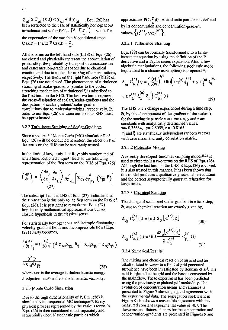
5-8

Xai 5 Cai (X,t) Xa i i- d Xai .@U. (26)has been restricted to the case of statistically homogeneous turbulence and scalar fields. (v I r,X ) stands for

the expectation of the variable V conditional upon C (x,t) = r and vC(x,t) = X .

-

- - All the terms on the left hand side (LHS) of Equ. (26) are closed and physically represent the accumulation of probability, the probability transport in concentration and concentration-gradient spaces due to chemical reaction and due to molecular mixing of concentrations, respectively. The terms on the right hand side (RHS) of Equ. (26) are not closed. The phenomenon of turbulence straining of scalar-gradients (similar to the vortex stretching mechanism of turbulence25) is adscribed to the first term on the RHS. The last two terms represent the cross-dissipation of scalars/scalar-gradients and the dissipation of scalar-gradiendscalar-gradient correlations due to molecular mixing, respectively. In order to use Equ. (26) the three terms on its RHS must be approximated.

3.2.2 Turbulence Straininp of Scalar-Gradients

Since a sequential Monte Carlo (MC) simulation27 of Equ. (26) will be conducted hereafter, the effect on P of the terms on the RHS can be separately treated.

In the limit of large turbulent Reynolds number and of small time, Kubo technique17 leads to the following representation of the first term on the RHS of Equ. (26).

The subscript 1 on the LHS of Equ. (27) indicates that the P variation is due only to the first term on the RHS of Equ. (26). It is pertinent to remark that Equ. (27) implies only mathematical approximations but no closure hypothesis in the classical sense.

For statistically homogeneous and isotropic fluctuating velocity-gradient fields and incompressible flows Equ. (27) finally becomes,

a2 P

where <E> is the average turbulent kinetic energy dissipation rate25 and v is the kinematic viscosity.

3.2.3 Monte Carlo Simulation

Due to the high dimensionality of P, Equ. (26) is simulated via a sequential MC techniqueu. Every physical process represented by the various terms in Equ. (26) is then considered to act separately and sequentially upon N stochastic particles which

approximate P(r, x ;t) . A stochastic particle n is defined by its concentration and concentration-gradient values, { C(n),(VC)(n)}.

- -

3.2.3.1 Turbulence Straining

Equ. (28) can be formally transformed into a fmite- increment equation by using the definition of the P derivative and a Taylor series expansion. After a few algebraic manipulations, the following stochastic model (equivalent to a closure assumption) is proposed34,

The LHS is the change experienced during a time step, &, by the ith component of the gradient of the scalar a for the stochastic particle n at time t. x, y and z are constants with analytically determined values,

q and 5 are statistically independent random vectors with zero mean and unity correlation matrix.

x=- 0.35634, y= 2.8059, z =- 0.8165

3.2.3.2 Molecular Mixinq

A recently developed binomial sampling mode13334 is used to close the last two terms on the RHS of Equ. (26). Although the last term on the LHS of Equ. (26) is closed, it is also treated in this manner. It has been shown that this model produces a qualitatively reasonable evolution and the correct asymptotically gaussian relaxation for large times.

3.2.3.3 Chemical Reaction

The change of scalar and scalar-gradient in a time step, &, due to chemical reaction are exactly given by,

3.2.4 Numerical Results

The mixing and chemical reaction of an acid and an alkali diluted in water in a field of grid generated turbulence have been investigated by Bennani et al5. The acid is injected at the grid and the base is convected by the main flow. These experiment has been predicted using the previously explained pdf methodoly. The evolution of concentration means and variances is presented in Figure 7 showing a good agreement with the experimental data. The segregation coefficient in Figure 8 also shows a reasonable agreement with the measured constant experimental value of -0.7. The skewness and flatness factors for the concentration and concentration-gradients are presented in Figures 9 and

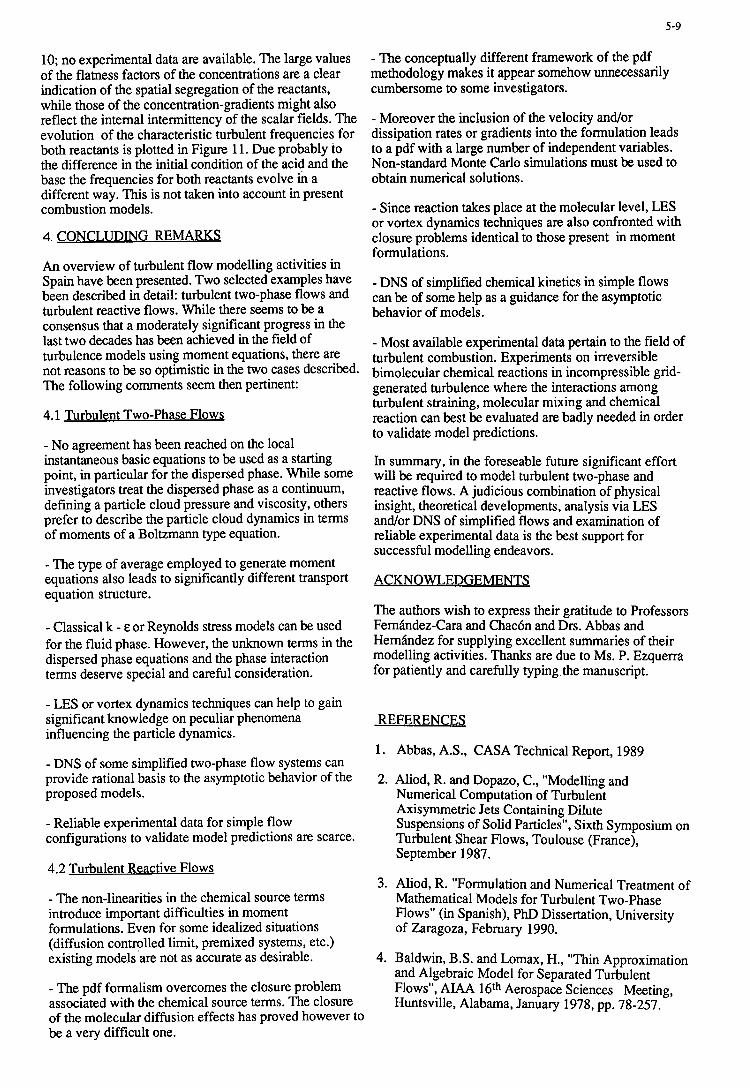
5-9

10; no experimental data are available. The large values of the flatness factors of the concentrations are a clear indication of the spatial segregation of the reactants, while those of the concentration-gradients might also reflect the intemal intermittency of the scalar fields. The evolution of the characteristic turbulent frequencies for both reactants is plotted in Figure 1 1. Due probably to the difference in the initial condition of the acid and the base the frequencies for both reactants evolve in a different way. This is not taken into account in present combustion models.

4. CONCLUDING REMARKS

An overview of turbulent flow modelling activities in Spain have been presented. Two selected examples have been described in detail: turbulent two-phase flows and turbulent reactive flows. While there seems to be a consensus that a moderately significant progress in the last two decades has been achieved in the field of turbulence models using moment equations, there are not reasons to be so optimistic in the two cases described. The following comments seem then pertinent:

4.1 Turbulent Two-Phase Flows

- No agreement has been reached on the local instantaneous basic equations to be used as a starting point, in particular for the dispersed phase. While some investigators treat the dispersed phase as a continuum, defining a particle cloud pressure and viscosity, others prefer to describe the particle cloud dynamics in terms of moments of a Boltzmann type equation.

- The type of average employed to generate moment equations also leads to significantly different transport equation structure.

- Classical k - E or Reynolds stress models can be used for the fluid phase. However, the unknown terms in the dispersed phase equations and the phase interaction terms deserve special and careful consideration.

- LES or vortex dynamics techniques can help to gain significant knowledge on peculiar phenomena influencing the particle dynamics.

- DNS of some simplified two-phase flow systems can provide rational basis to the asymptotic behavior of the proposed models.

- Reliable experimental data for simple flow configurations to validate model predictions are scarce.

4.2 Turbulent Reactive Flows

- The non-linearities in the chemical source terms introduce important difficulties in moment formulations. Even for some idealized situations (diffusion controlled limit, premixed systems, etc.) existing models are not as accurate as desirable.

- The pdf formalism overcomes the closure problem associated with the chemical source terms. The closure of the molecular diffusion effects has proved however to be a verv difficult one.

- The conceptually different framework of the pdf methodology makes it appear somehow unnecessarily cumbersome to some investigators.

- Moreover the inclusion of the velocity and/or dissipation rates or gradients into the formulation leads to a pdf with a large number of independent variables. Non-standard Monte Carlo simulations must be used to obtain numerical solutions.

- Since reaction takes place at the molecular level, LES or vortex dynamics techniques are also confronted with closure problems identical to those present in moment formulations.

- DNS of simplified chemical kinetics in simple flows can be of some help as a guidance for the asymptotic behavior of models.

- Most available experimental data pertain to the field of turbulent combustion. Experiments on irreversible bimolecular chemical reactions in incompressible grid- generated turbulence where the interactions among turbulent straining, molecular mixing and chemical reaction can best be evaluated are badly needed in order to validate model predictions.

In summary, in the foreseable future significant effort will be required to model turbulent two-phase and reactive flows. A judicious combination of physical insight, theoretical developments, analysis via LES and/or DNS of simplified flows and examination of reliable experimental data is the best support for successful modelling endeavors.

ACKNOWLEDGEMENTS

The authors wish to express their gratitude to Professors Femlndez-Cara and Chac6n and Drs. Abbas and Hemhndez for supplying excellent summaries of their modelling activities. Thanks are due to Ms. P. Ezquerra for patiently and carefully typingthe manuscript.

REFERENCES

1 . Abbas, A.S., CASA Technical Report, 1989

2. Aliod, R. and Dopazo, C., "Modelling and Numerical Computation of Turbulent Axisymmetric Jets Containing Dilute Suspensions of Solid Particles", Sixth Symposium on Turbulent Shear Flows, Toulouse (France), September 1987.

3. Aliod, R. "Formulation and Numerical Treatment of Mathematical Models for Turbulent Two-Phase Flows" (in Spanish), PhD Dissertation, University of Zaragoza, February 1990.

4. Baldwin, B.S. and Lomax, H., "Thin Approximation and Algebraic Model for Separated Turbulent Flows", AIAA 16th Aerospace Sciences Meeting, Huntsville, Alabama, January 1978, pp. 78-257.

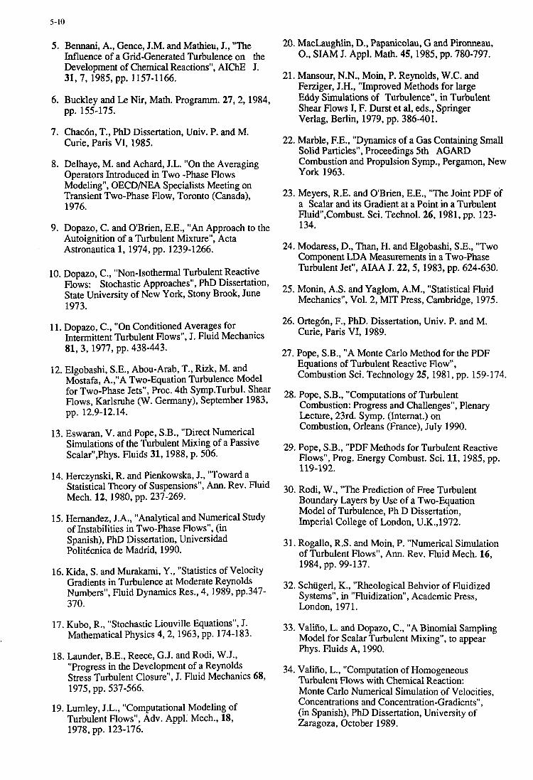
5-10

5. Bennani, A., Gence, J.M. and Mathieu, J., "The Influence of a Grid-Generated Turbulence on the Development of Chemical Reactions", AIChE J. 31,7, 1985, pp. 1157-1 166.

6. Buckley and Le Nir, Math. Programm. 27,2,1984, pp. 155-175.

7. Chach, T., PhD Dissertation, Univ. P. and M. Curie, Paris VI, 1985.

8. Delhaye, M. and Achard, J.L. "On the Averaging Operators Introduced in Two -Phase Flows Modeling", OECD/NEA Specialists Meeting on Transient Two-Phase Flow, Toronto (Canada), 1976.

9. Dopazo, C. and OBrien, E.E., "An Approach to the Autoignition of a Turbulent Mixture", Acta Astronautica 1, 1974, pp. 1239-1266.

10. Dopazo, C., "Non-Isothermal Turbulent Reactive Flows: Stochastic Approaches", PhD Dissertation, State University of New York, Stony Brook, June 1973.

11. Dopazo, C., "On Conditioned Averages for Intermittent Turbulent Flows", J. Fluid Mechanics 81,3 , 1977, pp. 438-443.

12. Elgobashi, S.E., Abou-Arab, T., Rizk, M. and Mostafa, A.,"A Two-Equation Turbulence Model for Two-Phase Jets", Proc. 4th Symp.Turbu1. Shear Flows, Karlsruhe (W. Germany), September 1983, pp. 12.9-12.14.

13. Eswaran, V. and Pope, S.B., "Direct Numerical Simulations of the Turbulent Mixing of a Passive Scalar",Phys. Fluids 31, 1988, p. 506.

14. Herczynski, R. and Pienkowska, J., "Toward a Statistical Theory of Suspensions", Ann. Rev. Fluid Mech. 12,1980, pp. 237-269.

15. Hernandez, J.A., "Analytical and Numerical Study of Instabilities in Two-Phase Flows", (in Spanish), PhD Dissertation, Universidad Politecnica de Madrid, 1990.

16. Kida, S . and Murakami, Y., "Statistics of Velocity Gradients in Turbulence at Moderate Reynolds Numbers", Fluid Dynamics Res., 4, 1989, pp.347- 370.

17. Kubo, R., "Stochastic Liouville Equations", J. Mathematical Physics 4,2 , 1963, pp. 174-183.

18. Launder, B.E., Reece, G.J. and Rodi, W.J., "Progress in the Development of a Reynolds Stress Turbulent Closure", J. Fluid Mechanics 68, 1975, pp. 537-566.

19. Lumley, J.L., "Computational Modeling of Turbulent Flows", Adv. Appl: Mech., 18, 1978, pp. 123-176.

20. MacLaughlin, D., Papanicolau, G and Pironneau, O., SIAM J. Appl. Math. 45,1985, pp. 780-797.

21. Mansour, N.N., Moin, P. Reynolds, W.C. and Ferziger, J.H., "Improved Methods for large Eddy Simulations of Turbulence", in Turbulent Shear Flows I, F. Durst et al, eds., Springer Verlag, Berlin, 1979, pp. 386-401.

22. Marble, F.E., "Dynamics of a Gas Containing Small Solid Particles", Proceedings 5th AGARD Combustion and Propulsion Symp., Pergamon, New York 1963.

23. Meyers, R.E. and OBrien, E.E., "The Joint PDF of a Scalar and its Gradient at a Point in a Turbulent Fluid",Combust. Sci. Technol. 26, 1981, pp. 123- 134.

24. Modaress, D., Than, H. and Elgobashi, S.E., "Two Component LDA Measurements in a Two-Phase Turbulent Jet", AIAA J. 22, 5, 1983, pp. 624-630.

25. Monin, A.S. and Yaglom, A.M., "Statistical Fluid Mechanics", Vol. 2, MIT Press, Cambridge, 1975.

26. Ortegh, F., PhD. Dissertation, Univ. P. and M. Curie, Paris VI, 1989.

27. Pope, S.B., "A Monte Carlo Method for the PDF Equations of Turbulent Reactive Flow", Combustion Sci. Technology 25, 1981, pp. 159-174.

28. Pope, S.B., "Computations of Turbulent Combustion: Progress and Challenges", Plenary Lecture, 23rd. Symp. (Internat.) on Combustion, Orleans (France), July 1990.

29. Pope, S.B., "PDF Methods for Turbulent Reactive Flows", Prog. Energy Combust. Sci. 11, 1985, pp. 119-192.

30. Rodi, W., "The Prediction of Free Turbulent Boundary Layers by Use of a Two-Equation Model of Turbulence, Ph D Dissertation, Imperial College of London, U.K.,1972.

31. Rogallo, R.S. and Moin, P. "Numerical Simulation of Turbulent Flows", Ann. Rev. Fluid Mech. 16, 1984, pp. 99-137.

32. Schiigerl, K., "Rheological Behvior of Fluidized Systems", in "Fluidization", Academic Press, London, 1971.

33. Valiiio, L. and Dopazo, C., "A Binomial Sampling Model for Scalar Turbulent Mixing", to appear Phys. Fluids A, 1990.

34. Valiiio, L., "Computation of Homogeneous Turbulent Flows with Chemical Reaction: Monte Carlo Numerical Simulation of Velocities, Concentrations and Concentration-Gradients", (in Spanish), PhD Dissertation, University of Zaragoza, October 1989.

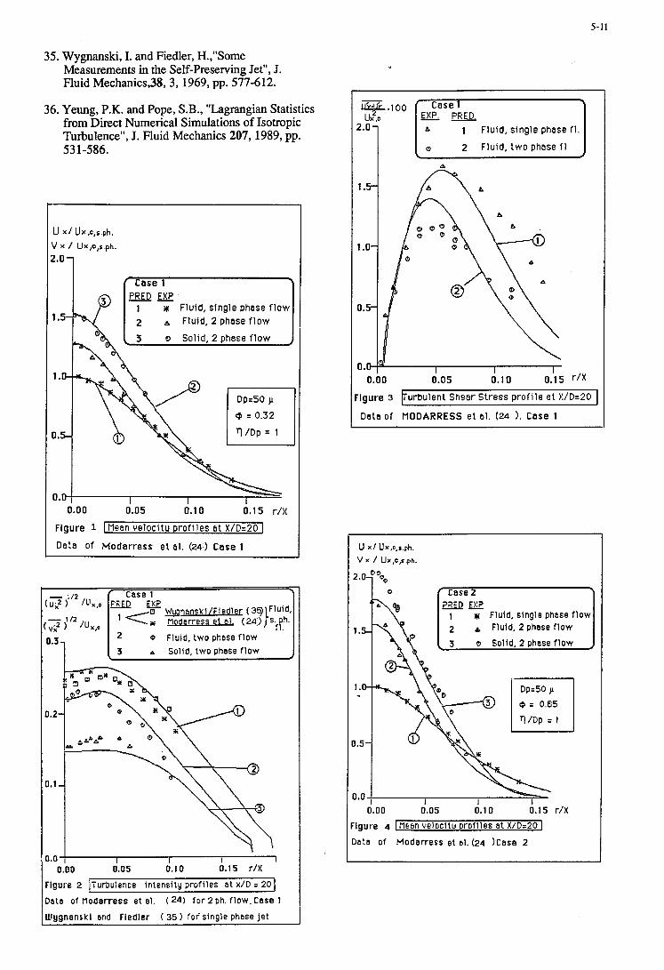
5-11

35. Wygnanski, I. and Fiedler, H.,"Some Measurements in the Self-Preserving Jet", J. Fluid Mechanics,38, 3, 1969, pp. 577-612.

36. Yeung, P.K. and Pope, S.B., "Lagrangian Statistics from Direct Numerical Simulations of Isotropic Turbulence", J. Fluid Mechanics 207, 1989, pp. 53 1-586.

! . O -

1.5-

1 .a

3.5-

0.0- I

Case 1 p IFRED EXP 1 Fluid, s ingle phase f l o w

I 2 A Fluid, 2 phase f l o w

3 D Solid, 2 phase f l o w

<\[

IO 0.05 0.1 0 0.15 r/X Figure 1 I Mean veTocitu p ro f i les a t X/D='LO I Data Of Modar ress e t al. (24) Case 1

2 v Fluid, two phase f low 3 A Solid, two phase f low

D.0 I I I 1 0.00 0.05 0.10 0.15 r / X

Figure 2 Turbulence intensity profi les a t x/D = 20 I 3 a t a of noderress e t 31. ( 24) f o r 2 ph. f low. Case 1

Ulygnanrki and Fiedler ( 35 ) l o t single phase j e t

Fluid, single phase fl.

2 Fluid, two phase I 1

0.00 0.05 0.10

' i gure 3 /Turbulent Shear Stress p ro f i l e a t #/D=20 I Data o f MODARRESS e t al. (24 ). Case 1

U x / Ux,c,r.ph.

v X / Ux,c,s.ph.

2.0

1.5

1 .o

3.5.

0.0

'Qo

Fluid, single phase f low A Fluid, 2 phase f low

JO 0.05 0.1 0 0.15 r/X rigure 4 [Hean velocitu Drofiles a t X/D=20 1 Data of Modarress e t al. (24 )Case 2

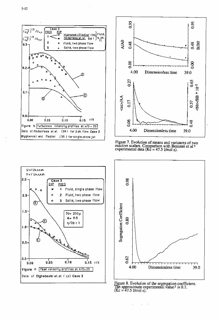
5-12

igure 5

2 0 Fluid, t w o phese f l o w 3 Solid, two phese f low

Turbulence intensi ty prof i les e t x/D = 20

U x/ Ux,c,s.ph.

V x / Ux,c,s.ph.

2.5

2.0

1.5.

I .o-

0.5-

3.0- I

E X P U 8 1 Fluid, s ingle phase f l o w

A 2 Fluid, t w o phase f l o w

Q 3 Solid, t w o phase f l o w

\ 1-

I i I 10 0.05 0.1 0 0.15

Figure 6 [Mean ve loc i ty p r o f i l e s a t X/D=20 I Date of Elghobashi e t a l . 12) Case 3

r/X

3)

4.00 Dimensionless time 39.0


Figure 7. Evolution of means and variances of two reactive scalars. Comparison with Benanni et a1 5 experimental data (Kc = 47.5 Vmol s).

"1 Y

.d 8 g 8 0 .d g o uoq

c)

2 00 0

r a

c\1

3 4.00 Dimensionless time 39.0

Figure 8. Evolution of the segregation coefficient. The ap roximate experimental values is 0.7. (KC = B7.5 Vmol SI.

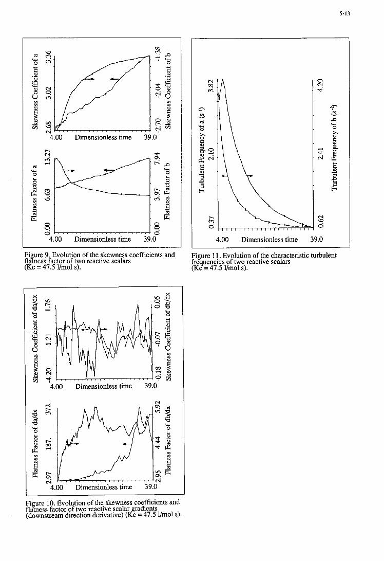
5-13

cd ru 0 Y

8

8

.- 4 U m

F 2

W

m c?

6

4

00

3 . 4.00 Dimensionless time 39.0

F

m w m

E d L L

8 . 23 0 ~ " " " " " " " " " " ' ~ 0


Figure 9. Evolution of the skewness coefficients and flatness factor of two reactive scalars (Kc = 47.5 Vmol s).

cj 4 % 3 ru 0 l-4

U 0 0 9 6 L 2 +

3 2 F 2

m m



Figure 1 i. Evolution of $e characteristic turbulent frequencies of two reactive scalars (Kc = 47.5 Ymol s).

Figure 10. Evolution of the skewness coefficients and flatness factor of two reactive scalar radients (downstream direction derivative) ( 2 c = 47.5 Ymol s).

i

1

I

I I

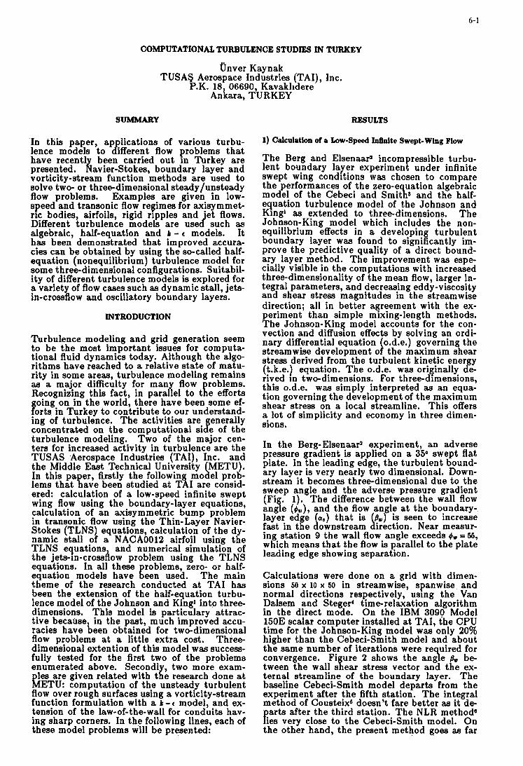
COMPUTATIONAL TURBULENCE STUDIES IN TURKEY

SUMMARY

tfnver Kaynak TUSAS Aerospace Industries (TAI), Inc.

P.K. 18 06690, Kavaklidere Ankara, TURKEY

RESULTS

In this paper, a p lications of various turbulence models t o Afferent flow problems tha t have recent1 been carried out in Turkey are

vorticity-stream function methods are used t o solve two- or three-dimensional steady/unsteady flow problems. Examples are given in low- speed and transonic flow regimes for axisymmetric bodies, airfoils, rigid ripples and 'et flows.

algebraic, half-equation and k - a models. It has been demonstrated tha t improved accuracies can be obtained by using the so-called half- equation (nonequilibrium) turbulence model for some three-dimensional configurations. Suitabil- ity of different turbulence models is explored for a variety of flow cases such as dynamic stall, jets- in-crossflow and oscillatory boundary layers.

presented. R avier-Stokes, boundary layer and

Different turbulence models are use d such as

INTRODUCTION

Turbulence modeling and grid generation seem t o be the most important issues for computational fluid dynamics today. Although the algo- rithms have reached to a relative state of matu- rity in some areas, turbulence modeling remains as a major difficulty for many flow roblems.

oing on in t he world, there have been some efforts in Turkey to contribute to our understanding of turbulence. T h e activities are enerally

turbulence modeling. Two of the major cen- ters for increased activity in turbulence are the TUSAS Aerospace Industries (TAI), Inc. and the Middle East Technical University METU).

ered: calculation of a low-speed infinite swept wing flow using the boundary-layer equations, calculation of an axisymmetric bump problem in transonic flow using the Thin-Layer Navier- Stokes (TLNS) equations, calculation of the dynamic stall of a NACA0012 airfoil using the TLNS equations and numerical simulation of t he jets-in-crosshow problem using the TLNS equations. In all these roblems, zero- or half-

The main theme of the research conducted at TA1 has been the extension of the half-equation turbulence model of the Johnson and King1 into three- dimensions. This model is particulary attrac- tive because in the past, much improved accuracies have been obtained for two-dimensional flow problems at a little extra cost. T h r e e dimensional extention of this model was successfully tested for t he first two of the problems enumerated above. Second1 , two more exam-

les are given related with t i e research done at hETU: computation of t he unsteady turbulent flow over rough surfaces using a vorticity-stream function formulation with a k - c model, and extension of the law-of-the-wall for conduits having sharp corners. In the following lines, each of these model problems will be presented:

Recognizing this fact, in parallel t o t R e efforts

concentrated on the computational si Cf e of the

In this pa er, firstly the followin mo a el problems tha t Rave been studied at T x I are consid-

equation models have ! een used.

1) Calculation of a Low-Sped W t e Swept-Wlng Flow

The Berg and Elsenaars incompressible turbulent boundary layer experiment under infinite swept wing conditions was chosen to compare the performances of t he zero-e uation algebraic model of the Cebeci and S m i h and the half- equation turbulence model of the Johnson and King1 as extended to three-dimensions. The Johnson-King model which includes the nonequilibrium effects in a developin turbulent boundary layer w a s found to signi a cantly improve the predictive quality of a direct boundary layer method. The improvement was especially visible in the computations with increased three-dimensionality of the mean flow, larger integral parameters, and decreasing eddy-viscosity and shear stress magnitudes in the streamwise direction; all in better agreement with the experiment than simple mixing-length methods. T h e Johnson-Kin6 model accounts for the convection and diffusion effects by solving an ordinary differential equation 0.d.e.) governing the streamwise development o the maximum shear stress derived from the turbulent kinetic ener y (;t.k.e.) equation. The 0.d.e. w a s originally dpe- rived in two-dimensions. For three-dimensions, this 0.d.e. waa simply interpreted aa an equation governing the development of the maximum shear stress on a local streamline. This offers a lot of simplicity and economy in three dimensions.

In the Berg-Elsenaar' experiment, an adverse pressure gradient is applied on a 35" swept flat plate. In the leading edge, t he turbulent boundary layer is very nearly two dimensional. Down- stream it becomes three-dimensional due to the

at the boundary- seen to increase

ing station 9 the wall flow angle exceeds Ow = 66, which means tha t the flow is parallel t o the plate leading edge showing separation.

Calculations were done on a grid with dimensions 60 x 10 x 60 in streamwise, spanwise and normal directions respectively, using the Van Dalsem and Steger' time-relaxation algorithm in the direct mode. On the IBM 3090 Model 150E scalar computer installed at TAI, the CPU time for the Johnson-King model was only 20% higher than the Cebeci-Smith model and about the same number of iterations were re uired for convergence. Fi ure 2 shows the a n g e 7 p., be-

ternal streamline of the boundary layer. The baseline Cebeci-Smith model departs from the experiment after the fifth station. The integral method of Cousteix* doesn't fare better as it de-

ar ts after t he third station. T h e NLR methods

the other hand, the present method goes as far

tween the wall s Yl ear stress vector and the ex-

P ies very close to the Cebeci-Smith model. On

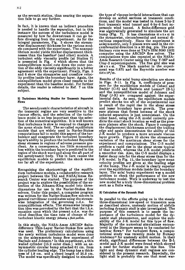
6-2

as the seventh station, than nearing the separation fails to go any further.

In fact, it is known tha t an indirect procedure is needed to handle the separation, but in this instance the success of the turbulence model is measured by how far downstream it can go before diverging from the experiment. As for t he

arameters, Fig. 3 shows the stream-

els compared with the experiment. T h e nonequilibrium model yields thicker displacement thicknesses than the baseling (and other) models. A turbulent eddy viscosity profile (at Station 7) is presented in Fi 4 which shows tha t t he

tion of the edd viscosity significantly in a better agreement wit K the experiment. Finally, Figs. 5 and 6 show the streamwise and crossflow velocity profiles inside the boundar layer. Again, the

experiment than the baseline model. For further details, the reader is referred to Ref. 7 on this subject .

wise disp P acement thickness for the various mod-

nonequilibrium mo % el cuts down the outer por-

nonequilibrium model gives c r oser results to the

1) "urbulence Modeling Studies for Transonic Separated Flows

The aerodynamic characteristics of aircraft in the transonic regime are very sensitive to the viscous effects, and the selection of the turbulence model is no less important than the selection of the numerical algorithm. It is well known tha t turbulence is slow to respond to changes in the mean strain field. The so-called equilibrium models t ha t are widely used in Navier-Stokes computations fail t o model this aspect of the turbulence and exaggerate the turbulent boundary layer's ability to produce the turbulent Reynolds s h e a stresses in regions of adverse pressure gradient. As a consequence, too little momentum loss within the boundary layer is predicted in the region of the shock wave and along the aft part of the aerodynamic body. This in turn causes the equilibrium models to predict the shock waves too far aft of the experiment.

Recognizing the shortcomings of the equilibrium turbulence models, a collaborative research project between the TA1 and NASA/Ames Re- search Center was started. The purpose of the project w a s t o explore the possibilities of the extention of t he Johnson-King model into three- dimensions for use in the Navier-Stokes flow solvers. Under this project, a computer program was written for t he Navier-Stokes flow solvers in general curvilinear coordinates using the streamwise integration of the governing 0.d.e. for nonequilibrium effects. The streamwise inte ra-

equation upon whlch the present 0.d.e. w a s derived describes the t ime rate of change of the turbulent kinetic energy following D fluid partide.

In this s tud , the NASA-Ames A R C 3 D finite- difference Tiin-Layer Navier-Stokes flow solver was used. The preliminary calculations using the newly written turbulence model were done on the axis mmetric bump flow experiment of

walled cylinder 15.2 outer diam.) with an ax-

t he cylinder leading edge. The bump has a thickness of 1.9 cm. and a chord length of 20.3 cm. The model w a s specifically designed to simulate

tion idea was provpked by the fact t ha t the t. 1 .e.

Bachalo an dy Johnson.9 In this experiment, a thin

isymmetric circu \ ar bump attached 61 cm. from

the t pe of viscous-inviscid interactions tha t can deveLp on airfoil sections at transonic conditions, and the model was tested in Ames 2-by-2 foot transonic wind tunnel and 6-b -6 foot supersonic wind tunnel. A Bnite-di fty erence grid was a1 ebraically enerated to simulate the arc bump $Fig. 7). B t has dimensions 61 x 5 x 41 in the streamwise, circumferential and normal directions respective1 . Since the expqriment is axisymmetric, only planes were used in the circumferential direction in a 90 deg. pie. The preliminary runs were done at TAI's IBM 3090 150E computer using the ARC3D flow solver. T h e computations were also repeated at the NASA- Ames Research Center usin the Cray Y-MP and Cray-2 supercomputers. T a e fine grid size waa 1 3 8 ~ 6 x 4 6 . The Mach number in the experiment w a s 0.875 and the Reynolds number w a s 13.6 x los/m.

Results of the axial bump simulation are shown in Figs. 8-11. In Fig. 8, coefficients of pressure for the equilibrium models of Cebeci and Smith8 (C-S) and Baldwin and Lomaxlo (B-LJ and the nonequilibrium model of Johnson an King1 J-K) are compared against the exper-

predict shocks too aft of the experimental one in result of the rapid rise in the shear stress and lesser boundary layer growth. The pressure plateau tha t forms because of t he shock induced separation is just nonexistent. On the other hand, using the J-K model correctly predicts the exact shock location as well as the pressure plateau after the shock. Figure 9 compares the displacement thicknesses around the trailing ed e and again demonstrates the ability of the J-k model to produce a more accurate viscous layer krowth. Figure 10 shows the streamwise variation of the maximum shear stress for the experiment and computations. The C-S model predicts a ra id rise in the shear stress t y ical of tha t mode!, whereas the J-K model pre B icts a smoother rise. Also the C-S model displays a faster decay rate for the shear stress than for the J-K model. In Fig. 11, the boundary layer mean velocit profiles are iven at the trailing edge

over the equilibrium models inside the boundary layer. The axial bump experiment w a s a model problem to check the erformance of the new

new model for a truly three-dimensional problem such as a finite wing.

3) Calculatlon of the Dynamlc Stall

In parallel to the efforts going on in the steady three-dimensional low-speed or transonics area as described above, unsteady motion of airfoils including dynamic stall is also investigated. The purpose of this research is to assess the importance of the turbulence model for the dynamic stall phenomenon and explore the suitability of the J-K modei for this type of flow. Majority of the numerical simulations encountered in the literaure seems to be conducted for laminar flows.11 For turbulent flows, a computational study w a s recently made by Rumsey Anderson12 for unsteady airfoil motion. In their study, significant differences between the B-L model and J-K model were found which showed a need for further studies on this line. T h e light and deep dynamic stall re imes are considered in the present research. 5 specially, t he light stall is probably the one tha t most war-

imenta I data. As seen, the equilibrium models

of the 1: ump. The J-I? model is clearly superior

turbulence model. Wor kp is underway to test the

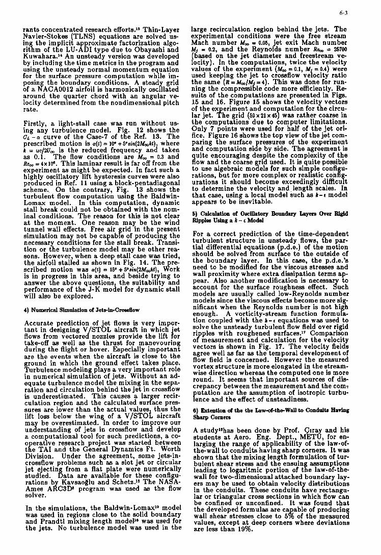
6-3

rants concentrated research efforts.*$ Thin-Layer Navier-Stokes (TLNS) equations are solved usin the implicit ap roximate factorization algo- ri&m of the LU-A81 type due to Obayashi and Kuwahara.1' An unsteady version w a s developed by including the t ime metrics in the program and usin the unsteady normal momentum equation

the boundary conditions. A steady grid $?#ACA0012 airfoil is harmonically oscillated around the quarter chord with an angular velocity determined from the nondimensional pitch rate.

for t a e surface pressure computation while im-

Firstly, a light-stall case w a s run without using any turbulence model. Fig. 12 shows the CL - a curve of the Case-7 of the Ref. 13. The prescribed motion is a(t) = l(P + S08in(2M,kt), where k = wc/2Um is the reduced frequency and taken as 0.1. T h e flow conditions are M , = 0.3 and R b = 4xlOd. This laminar result is far off from the experiment as might be expected. In fact such a highly oscillatory lift hysteresis curves were also produced in Ref. 11 using a block-pentadiagonal scheme. On the contrary, Fig. 13 shows the turbulent flow computation using the Baldwin- Lomax model. In this computation, dynamic stall break could not be obtained with the nom- inal conditions. The reason for this is not clear at the moment. One reason may be the wind tunnel wall effects. Free rid in the present simulation ma not be ca of producing the

tion or the turbulence model may be other reasons. However, when a deep stall case was tried, t he airfoil stalled as shown in Fig. 14. The re- scribed motion w a s a(t) = 1 5 O + 5'8in(2~,~), $ork is in progress in this area, and beside trying to answer the above questions, t he suitability and performance of the J-K model for dynamic stall will also be explored.

4) Numerlcal Simulation of Jete-in-Croeeflow

Accurate prediction of jet flows is very impor- tan t in designing V STOL aircraft in which jet

take-off as well as the thrust for manevouring during the flight or hover. Especially important are the events when the aircraft is close to the ground in which the ground effect takes place. Turbulence modeling plays a very im ortant role

equate turbulence model the mixing in the separation and circulation behind the jet in crossflow is underestimated. This causes a lar er recir-

sures are lower than the actual values thus the lift loss below the wing of a V/STOL aircraft ma be overestimated. In order t o im rove our un J erstanding of jets in crossflow an! develop a computational tool for such predictions, a co- o erative research project was started between t i e TA1 and the General Dynamics Ft. Worth Division. Under the agreement, some jets-in- crossflow problems such aa a slot jet or circular jet ejectin from a flat plate were numerically

rations b Kavsaoglu and Schetz.16 The NA A- Ames AFkX3DB program w a s used as the flow solver.

In the simulations, the Baldwin-LomaxIo model w a s used in regions close to the solid boundary and Prandtl mixing length model16 w a s used for the jets. No turbulence model w a s used in the

necessary condkions for break. Transi-

flows from vectore d nozzles provide the lift for

in numerical simulation of jets. Wit R out an ad-

culation region and the calculated sur B ace pres-

sf studied. % ata are available for these conA u-

large recirculation region behind the jets. T h e experimental conditions were the free stream Mach number M, = 0.06, jet exit Mach number Mr = 0.2, and the Reynolds number R h = 26700 (based on the jet diameter and freestream velocity). In the computations, twice the velocity values of the experiment (Mm = 0.1, M = 0.4) were used keeping the je t t o crossflow veiocity ratio the same ( R = M , / M =4) . This w a s done for run- ning the compressible code more efficiently. Re- sults of the computations are presented in Figs. 15 and 16. Figure 15 shows the velocity vectors of the ex eriment and com utation for t he circular jet. {he grid (59 x21 XG! was rather coarse in the computations due to computer limitations. Only 7 points were used for half of the j e t orifice. Figure 16 shows the top view of the jet comparing the surface ressures of the experiment

quite encouraging despite the complexity of the flow and the coarse rid

rations, but for more complex or urations it should become t o determine the velocity and length scales. In tha t case, using a local model such as k-e model appears t o be inevitable.

S) Calculation of Oscillatory Boundary Layem Over Rigid Ripplea Using a k - E Model

For a correct prediction of the time-dependent turbulent structure in unsteady flows, the partial differential equations p.d.e.) of t he motion should be solved from sur r ace to the outside of the boundary la er. In this case, t he p.d.e.'s

wall proximity where extra dissipation terms appear. Also another modification is necessar t o account for the surface roughness effect. &ch models are usually called low-Reynolds number models since the viscous effects become more significant when the Reynolds number is not hi h

tion coupled with the k - c equations w a s used to solve the unsteady turbulent flow field over rigid ri ples with roughened surfaces.17 Comparison

vectors is shown in Fig. 17. The velocity flelds agree well as far aa the temporal development of flow field is concerned. However the measured vortex structure is more elongated in the streamwise direction whereas the computed one is more round. I t seems tha t important sources of discrepancy between the measurement and the comt putation are the assumption of isotropic turbulence and the effect of unsteadiness. 6) Extention of the the Law-of-the-Wall to Conduits Having Sharp Cornera

A studylahas been done by Prof. Q r a y and his students at Aero. Eng. De t., METU, for en-

the-wall to con dg uits having sharp corners. It was shown tha t the mixing length formulation of turbulent shear stress and the ensuin assumptions

wall for two-dimensional attached boundary layers may be used t o obtain velocit distributions

lar or trian ular cross sections in which flow can

the developed formulas are ca able of producin wall shear stresses close to 5 8 of the meaaure values, except at deep corners where deviations are less than 19%.

and computation si B e by side. The agreement is

t o use algebraic mo 5 els

need to be modi l ed for the viscous stresses and

enough. A vorticity-stream function formu k a-

o P measurement and calculation for the velocity

larging the ran e of applica E ility of t h e law-of-

leading to logaritmic portion of t a e law-of-the-

in the conduits. These conduits z ave rectangu-

be confine % or unconfined. I t was found tha t

d

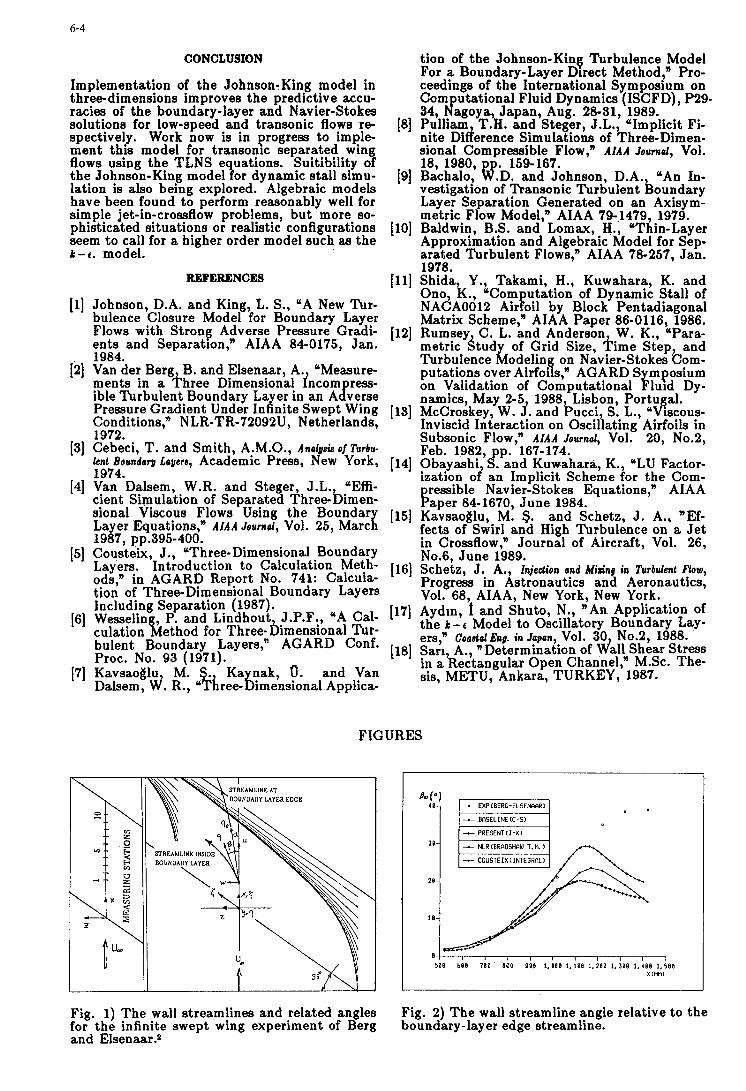
6-4

CONCLUSION

Implementation of t he Johnson-King model in three-dimensions improves the predictive accuracies of the boundary-layer and Navier-Stokes solutions for low-speed and transonic flows respectively. Work now is in progreaa t o imple- ment this model for transonic separated wing flows using the TLNS e uations. Suitibility of

lation is also being explored. Algebraic models have been found to perform reasonably well for simple jet-in-croasflow problems, but more so- phisticated situations or realistic configurations seem to call for a higher order model such as t he k-c. model.

the Johnson-King model 9 or dynamic stall simu-

REFERENCES

[l] Johnson, D.A. and King, L. S., “A New Tur- bulence Closure Model for Boundary Layer Flows with Strong Adverse Pressure Gradi- ents and Separation,” AIAA 84-0175, Jan. 1984.

[2) Van der Berg B. and Elsenaar, A. “Measure- ments in a ‘khree Dimensional incom ress-

Conditions,” NLR-TR-72092U, Netherlands, 1972.

[3] Cebeci, T. and Smith, A.M.O., Andy& of Turbu- lent Boundor! Loyere, Academic Press, New York, 1974.

[4] Van Dalsem, W.R. and Steger, J.L., “Effi- cient Simulation of Separated Three-Dimen- sional Viscous Flows Using the Boundary Layer Equations,” A I A A Journal, Vol. 25, March

[SI Cousteix, J., “Three-Dimensional Boundary Layers. Introduction to Calculation Meth- ods: in AGARD Report No. 741: Calcula- tion of Three- Dimensional Boundary Layers Including Separation (1987).

P. and Lindhout J.P.F., “A Cal- culation het hod for Three-bimensional Tur- bulent Boundary Layers,” AGARD Conf. Proc. No. 93 (1971).

[7] Kavsaoglu M. S. Ka nak, 0. and Van Dalsem, d. R., “Three-bimensional Applica-

ible Turbulent Boundary La er in an A 8 verse Pressure Gradient Under In il nite Swept Wing

1987, pp.395-400.

[SI Wesselin

tion of t he Johnson-King Turbulence-Model For a Boundary-Layer Direct Method,” Pro- ceedings of t he International Symposium on Com utational Fluid Dynamics (ISCFD), P29-

Pulliam, T.H. and Steger, J.L., “Implicit Fi- nite Difference Simulations of Three-Dimen- sional Compressible Flow,” AIAA Journal. Vol.

34, If agoya, Japan, Aug. 28-31, 1989.

18, 1980, @ 159-167. Bachalo, D. and Johnson, D.A.. “An In- vestigation of Transonic Turbulent Boundary Layer Separation Generated on an Axisym- metric Flow Model,” AIAA 79-1479, 1979. Baldwin, B.S. and Lomax, H., “Thin-Layer Approximation and Algebraic Model for Sep- arated Turbulent Flowa,” AIAA 78-257, Jan. 1978. Shida Y., Takami, H., Kuwahara, K. and Ono, k., ‘Com utation of Dynamic Stall of NACA0012 Airfoil by Block Pentadiagonal Matrix Scheme,” AIAA Paper 86-0116, 1986. Rumsey C. L. and Anderson W. K., “Para- metric dtud of Grid Size, &me Step, and

putations over Airfojs,” AGARD S mposium

namics, May 2-5, 1988, Lisbon, Portugal. McCroskey, W. J. and Pucci, S. L., “Viscous- Inviscid Interaction on Oscillating Airfoils in Subsonic Flow,” AIAA Journal, Vol. 20, No.2, Feb. 1982, p. 167-174. Obayashi, 8 and Kuwahara, K., “LU Factor- ization of an Implicit Scheme for the Com-

ressible Navier-Stokes Equations,” AIAA baper 84-1670, June 1984. Kavsaotlu, M. S. and Schetz, J. A., ”Ef- fects of Swirl and High Turbulence on a Jet in Crossflow,” Journal of Aircraft, Vol. 26, No.6, June 1989. Schetz, J. A., Injection and Mizing in Turbulent Now, Progress in Astronautics and Aeronautics, Vol. 68, AIAA, New York, New York. Aydin, 1 and Shuto, N., “An Application of the k - c Model t o Oscillatory Boundary Lay- ers,” CoaetelEng. in Japan, vol. 30 No.2, 1988. Sari, A., “Determination of d a l l Shear Stress in a Rectangular Open Channel,” M.Sc. The- sis, METU, Ankara, TURKEY, 1987.

Turbulence L odelin on Navier-Stokes Com-

on Validation of Computational $ luid Dy-

FIGURES

Fig. 1) The wall streamlines and related angles for the infinite swept wing experiment of Berg and Elsenaar.2

I 1 -+- PRESENTCJ-Kl I

580 b0E 701 800 908 1.100 1,188 1,200 1, I08 1.188 1,508 xtnni

Fig. 2) The wall streamline angle relative to the boundary-layer edge Streamline.

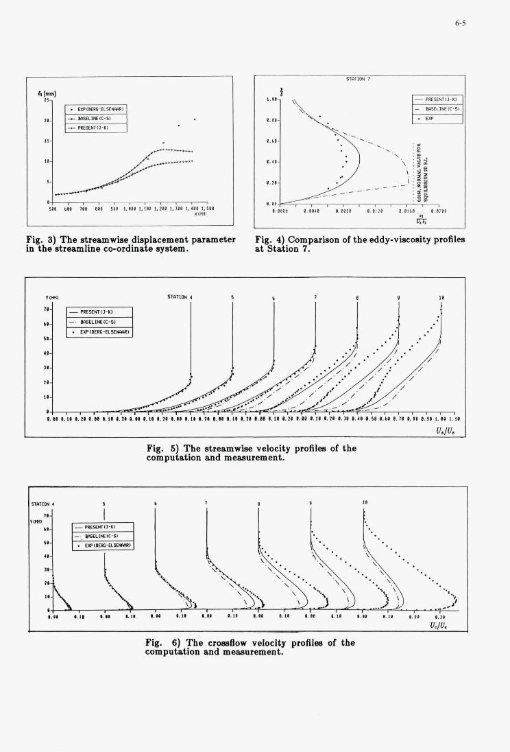
Fig. 8) The streamwise din lseement parameter in the streamline eo-ordina P e sysbm.

.. I

Fig. 4) Comparison of the eddy-vkosity profiles at Station 7.

lU" 6 b 1 II

1.11 1.11 1.11 1.11 1.11 1.18 1.11 1.11 1.11 1.11 1.11 1.21 1.11 1. I1 1.N 1.11 1.11 1.21 1.11 1.11 1.11 1.24 1.11 1.81 1.b1 1.11 1.11 t.0 1. I1 1.11

u.p. J Fig. 6 The streamwise velocity profiles of the compu 1 ation and measurement.

Fig. 6) The crosaflow velocity profiles of the computation and messurement.

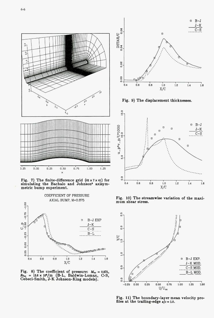
6-6

0

01 x " 0.'

Fig. B) The displacement thicknesses.

3125 0100 0:25 0:50 0175 I:OO 1.15 X

Fig. 7) The finite-difference grid (61 x 7 x 41) for simulating the Bachalo and Johnson' axisymmetric bump experiment.

COEFFICIENT OF PRESSURE AXIAL BUMP, M=0.875

0.4 0.8 0.8 1.2 I .4 1.8

Fig. 8) The coeficient of pressure: Mm = OHS, RC, = la6 x iV/m B-L, Baldwin-Lomax, CS, Cebeci-Smith, J-K \ ohnson-King models).

- d l , I

0.4 0.8 0.8 1.0 1.2 1.4 1.8

x/c

Fig. 10) The streamwise variation of the maximum shear stress.

R :I 0 E-JEXP.

J-K MOD. C-S MOD. __.___._______ B-L MOD.

x 1 -0.25 0.00 0.26 0.50 0.75 1.00 1.25 1.50

U/vm

Fig. 11) The boundary-layer mean velocity pro- 51- at the trailing-edge ;/e= LO.

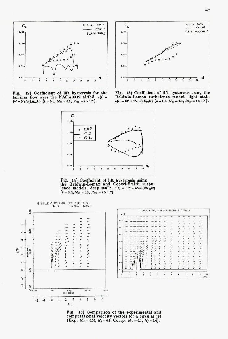
CL

""1

d

Fig. 12) Coefecient of Lit h steresia for the laminar Bow over the NACAO i 12 airfoil, n(t) - ID.+P~~ZM&) (j-ai, y.=od, h d x i 0 ' ) .

c,

C-5

0 - 0 W P .

(R-L MODEL =L. COHR

""1

13) Coefficient of lift hystereab using the %dwin-Lomax turbulence model, light stall: u(1) I 10. +6'r*(W&) (k = 0.1, M, = 0.8, Rc, = 4 X IC).

*a, .. . * -

1.11 -1 , , , , , , , , , , d I * I b I U $ I 1' 1h IO 21

Fig. 14) CoefRcient of lift h stereah using the Baldwin-Lomax and Cegeci-Smith turbulence models, deep stall: u(t) = 16. + 6%n(Wmkt) ( k = O.E,N, = 09, aC, = 4 x 10').

6-7

I I

I I I / , , I ,

~ - 3%

I , I , I , , , , , . - - - L

- 2 - 1 0 1 2 3 4 5 6 7 XA

Fig. 15) Comparison of the experimental and computational velocity vectom for a circular et (Exp: M- = 0.05, M, = 03; Comp: Mm = 0.1, = 0.4 J .

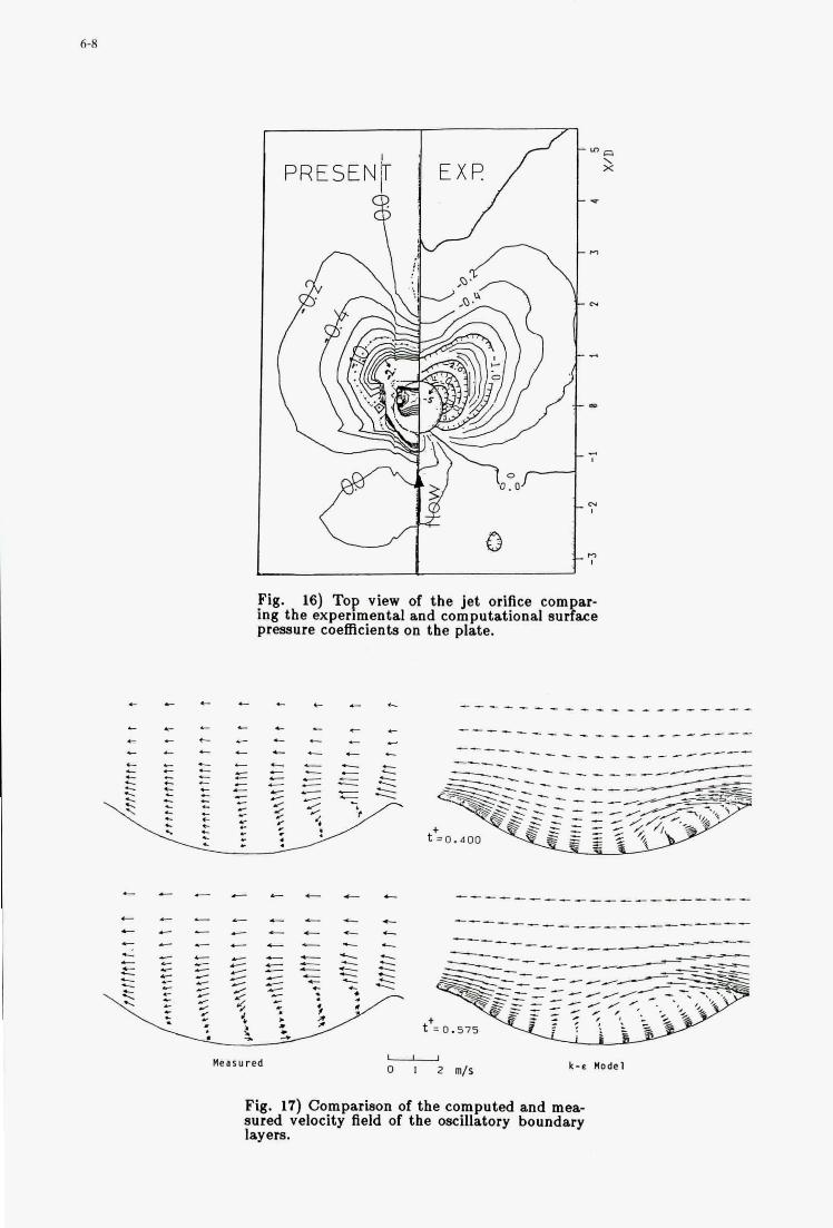
I 1

Fig. 16) Top view of the jet orifice com ar- ing the experimental and computational nu $ we pressure coemcienta on the plate.

6-E)

. - . - - _ C C C C L

+ . - C L C L C C

c c - - c c * c . - c c c c c - -

Measured k-e Wadel

Fig. 17) Comparison of the computed and measured velocity field of the oscillatory boundary layers.

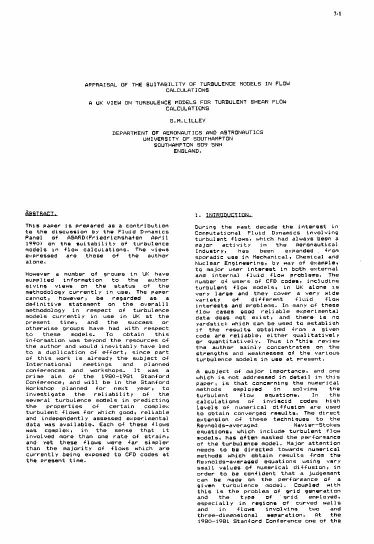
7-1

APPRAISAL OF THE SUITABILITY OF TURBULENCE MODELS IN FLOW CALCULATIONS

A UK VIEW ON TURBULENCE MODELS FOR TURBULENT SHEAR FLOW CALCULATIONS

G. M. L I LLEY

DEPARTMENT OF AERONAUTICS AND ASTRONAUTICS UNIVERSITY OF SOUTHAMPTON

SOUTHAMPTON SO9 5NH ENGLAND.

Th is paper i s prepared as a c o n t r i b u t i o n t o the d iscuss ion by t h e F l u i d Dynamics Panel of AGARD(Friedrichshafen A p r i l 1990) on t h e s u i t a b i l i t y of turbulence models i n f l ow ca l cu la t i ons . The views expressed are those o f t h e author alone.

However a number of groups i n UK have suppl ied i n fo rma t ion t o the author g i v i n g views on t h e s t a t u s o f t he methodology cur ren t1 y i n use. The paper cannot, however, be regarded as a d e f i n i t i v e statement on t h e o v e r a l l 1 methodology i n respect of turbulence models c u r r e n t l y i n use i n UK a t t he present t ime, and t h e succe6s or otherwise groups have had w i t h respect t o these models. To ob ta in t h i s in fo rmat ion was beyond t h e resources o f t h e author and would i n e v i t a b l y have l e d t o a d u p l i c a t i o n of e f f o r t , s ince p a r t o f t h i s work i s a l ready t h e sub jec t of I n t e r n a t i o n a l meetings and planned conferences and workshops. It was a prime aim of t h e 1980-1981 Stanford Conference, and w i l l be i n the Stanford Workshop planned f o r next year, t o i n v e s t i g a t e t h e r e l i a b i l i t y o f t h e severa l turbulence models i n p r e d i c t i n g t h e p roper t i es o f c e r t a i n complex tu rbu len t f l ows f o r which good, r e l i a b l e and independent1 y assessed experimental data was ava i lab le . Each o f these f lows was complex, i n t h e sense t h a t i t invo lved more than one r a t e o f s t r a i n , and yet these f l ows were f a r s impler than t h e m a j o r i t y of f l ows which are c u r r e n t l y being exposed t o CFD codes a t t he present t ime.

1. I N T R O D U C I m

During the past decade t h e i n t e r e s t i n Computational F l u i d Dynamics i n v o l v i n g tu rbu len t f lows, which had always been a major a c t i v i t y i n t h e Aeronautical Indus t ry , has been expanded , from sporadic use i n Mechanical, Chemical and Nuclear Engineering, by way o f example, t o major user i n t e r e s t i n both ex terna l and i n t e r n a l f l u i d f l ow problems. The number of users o f CFD codes, i n c l u d i n g tu rbu len t f low models, i n UK alone is very l a r g e and they cover a very wide v a r i e t y of d i f f e r e n t f l u i d f l ow i n t e r e s t s and problems. I n many o f these f l ow cases good r e l i a b l e experimental data does no t e c i s t , and the re i s no yards t ick which can be used t o e s t a b l i s h i f t h e r e s u l t s obtained from a g iven code are r e l i a b l e , e i t h e r q u a l i t a t i v e l y o r q u a n t i t a t i v e l y . Thus i n ' t h i s review t h e author main1 y concentrates on the s t rengths and weaknesses of t h e var ious turbulence models i n use a t present.

A sub jec t o f major importance, and one which i s no t addressed i n d e t a i l i n t h i s paper, i s t h a t concerning t h e numerical methods employed i n so l v ing the tu rbu len t f l ow equations. I n the c a l c u l a t i o n s o f i n v i s c i d codes h igh l e v e l s of numerical d i f f u s i o n are used t o ob ta in converged r e s u l t s . The d i r e c t extension of these techniques t o t h e Reynol ds-averaged Navi er-Stokes equations, which i nc lude tu rbu len t f low models, has o f t e n masked t h e performance o f t h e turbulence model. Major a t t e n t i o n needs t o be d i rec ted towards numerical methods which ob ta in r e s u l t s from t h e Reynolds-averaged equations us ing very small values of numerical d i f f u s i o n , i n order t o be conf ident t h a t a judgement can be made on t h e performance o f a g iven turbulence model. Coupled w i th t h i s is t h e problem of g r i d generat ion and t h e type o f g r i d employed, espec ia l l y i n reg ions o f curved w a l l s and i n f lows i n v o l v i n g two and three-dimensional separation. A t t h e 1980-1981 Stanford Conference one o f t h e

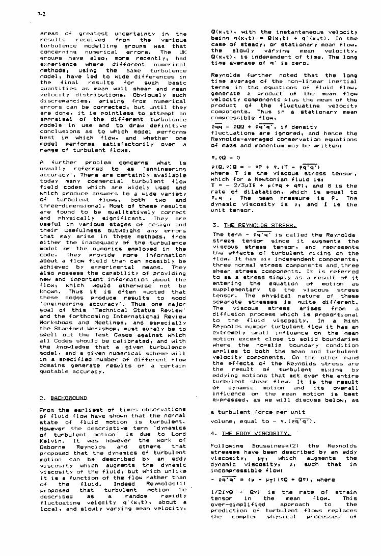
1-2

areas of greatest uncertainty in the results received from the various turbulence modelling groups was that concerning numerical errors. The UC: groups have also, more recently, had experience where different numerical methods, usi ng the same turbulence model, have led to wide differences in the final results for such basic quantities as mean wall shear and mean velocity distributions. Obviously such discrepancies, arising from numerical errors can be corrected, but until they are done, it is pointless to attempt an appraisal of the different turbulence models in use and to draw definitive conclusions as to which model performs best in which flow, and whether one model performs satisfactorily over a range of turbulent flows.

A further problem concerns what is usual 1 y ref erred to as 'engineering accuracy'. There are certainly available today many commercial turbulent flow field codes which are widely used and which produce answers to a wide variety of turbulent flows, both two and three-dimensional. Most of these results are found to be qualitatively correct and physically significant. They are useful in various stages of design and their usefulness outweighs any errors that may arise in these methods, from either the inadequacy of the turbulence model or the numerics employed in the code. They provide more information about a flow field than can possibly be achieved b y experimental means. They also possess the capability of providing new and important information about the flow, which would otherwise not be known. Thus it is often quoted that these codes produce results to good 'engineering accuracy'. Thus one major goal of this 'Technical Status Review' and the forthcoming International Review Workshops and Meetings, and especially the Stanford Workshop, must surely be to spell out the Test Cases against which all Codes should be calibrated, and with the knowledge that a given turbulence model, and a given numerical scheme will in a specified number of different flow domains generate results of a certain quotable accuracy.

2. B A W G R Q ! U R

From the earliest of times observations of fluid flow have shown that the normal state of fluid motion is turbulent. However the descriptive term ' dynamics of turbulent motion' is due to Lord Kelvin. It was however the work of Osborne Reynolds and others that proposed that the dynamics of turbulent motion can be described b y an eddy viscosity which augments the dynamic viscosity of the fluid, but which unlike it is a function of the flow rather than of the fluid. Indeed Reynolds(1) proposed that turbulent motion be described as a random rapidly fluctuating velocity q' (x,t), about a local, and slowly varying mean velocity,

Q(x,t), with the instantaneous velocity being q(x,t) = Q(x,t) + q'(x,t). In the case of steady, or stationary mean flow, the slowly varying mean velocity, Q(x,t), is independent of time. The long time average of q' is zero.

Reynolds further noted that the long time average of the non-linear inertial terms in the equations of fluid flow, generate a product of the mean flow velocity components plus the mean of the product of the f luctuating velocity components. Thus in a stationary mean compressible f 1 ow, p G = pQQ + Qq'q', if density fluctuations are ignored, and hence the Reynol ds-averaged conservation equations of mass and momentum may be written:

V . p Q = 0 P ( Q . V ) Q = - OF + 0. (1 - Pq'q') where T is the viscous stress tensor, which for a Newtonian fluid is: T I - 2/3pI8 + p ( v q + qv), and 0 is the rate of dilatation, which is equal to v.q . The mean pressure is P. The dynamic viscosity is p , and I is the unit tensor.

-

-

3. JHF RFYNnl nS STRFSS, - The term - pq'q' is called the Reynolds stress tensor since it augments the viscous stress tensor, and represents the effects of turbulent mixing on the flow. It has six independent components, three normal stress components and, three shear stress components. It is referred to as a stress simply as a result of it entering the equation of motion as supplementary to the viscous stress tensor. The physical nature of these separate stresses is quite different. The viscous stress arises from a diff~ision process which is proportional to the fluid viscosity. In a high Reynolds number turbulent flow it has an extremely small influence on the mean motion except close to solid boundaries where the no-slip boundary condition applies to both the mean and turbulent velocity components. On the other hand the effects of the Reynolds stress are the result of turbulent mixing b y eddying motions that act over the entire turbulent shear flow. It is the result of dynamic motion and its overall influence on the mean motion is best expressed, as we will discuss below, as

a turbulent force per unit

volume, equal to - 0 . (Qq'q'). I_

4. - ' FOllOWinQ Roussinesq(2) the Reynolds stresses have been described by an eddy viscosity, p ~ , which augments the dynamic visco6ity, p , such that in incompressible flow: - pq'q' = ( p + p ~ ) ( V Q + Q v ) , where

1 / 2 1 V Q + Q v ) is the rate of strain tensor in the mean flow. This over-simplif ied approach to the prediction of turbulent flows replaces the complex physical processes of

-

7-3

t u rbu len t mix ing by a s i n g l e sca la r parameter, p ~ , represent ing the tu rbu len t motion. A t bes t p i can be found exper imenta l l y, bu t t h i s presents d i f f i c u l t i e s s ince p~ i s f l ow dependent and v a r i e s i n magnitude throughout the tu rbu len t shear f low. I n general t he concept o f an eddy v i s c o s i t y i s app l ied on ly t o t h e shear s t ress components and no t t o t h e normal s t ress components. The s u m of t h e normal s t r e s s components i s p ropor t i ona l t o t h e mean k i n e t i c energy of t he tu rbu len t motion, and i f k i s t he mean k i n e t i c energy o f t h e tu rbu len t f l ow per u n i t mass then:

I n the I:-€ model p~ = Cppl::2/€ 9 no t i ng t h a t i s a l eng th sca le o f t h e turbulence.

Since i n t h e e a r l y p a r t o f t h i s century the Reynolds s t resses had no t been measured t h e on ly way open t o model t u r b u l e n t f l ows and thereby t o e f f e c t p red ic t i ons , was t o use dimensional ana lys i s and phys ica l arguments i n the determinat ion o f p ~ . I f VT = p ~ / p = O ( q l 3 , where q and 1 are c h a r a c t e r i s t i c sca les o f t u rbu len t v e l o c i t y and eddy s ize , and VT i s a p o s i t i v e quant i t y , then according t o Prandt l ( 3 ) 's mixing l eng th theory of turbulence, i n which t h e c h a r a c t e r i s t i c t u rbu len t v e l o c i t y was pu t equal t o 1 t imes the l o c a l mean shear, VT = I12dU/dyl i n a f l ow dominated by a mean shear dU/dy. Prandt l and o thers found t h i s model of turbulence s a t i s f a c t o r y i n many simple p r a c t i c a l f lows, prov ided the mixing length, 1, was s u i t a b l y chosen. I n the reg ion c lose t o t h e wa l l o f a tu rbu len t boundary l aye r von Karman proposed t h a t 1 = K y , whereas i n t h e outer reg ion o f t h e boundary l aye r , 1 i s a f r a c t i o n o f t h e mean boundary l aye r thickness. I n f r e e shear f lows, such as wakes, j e t s and mix ing reg ions Prandt l proposed t h a t t h e c h a r a c t e r i s t i c t u rbu len t v e l o c i t y should be p ropor t i ona l t o the v e l o c i t y d i f f e rence across t h e shear l aye r and 1 was p ropor t i ona l t o t h e l o c a l mean width of t he shear l aye r . A l l these r e s u l t s were supported by f low v i s u a l i s a t i o n and observation. The aim throughout was t o p red i c t t h e mean ve l o c i t y d i s t r i but i on, although i n most cases t h i s became a post -d i c t i on s i nce t h e emp i r i c a l constants i n t h e mix ing l eng th formulas had t o be pre-determined from

experiment. Other forms o f t h e mix ing l eng th theory of turbulence were in t roduced, such as t h e v o r t i c i t y

' t r a n s p o r t theory o f G. I .Tay lor (4) 9 w i t h s i m i 1 ar success.

Fo l low ing t h e i n t r o d u c t i o n o f t h e ho tw i re , measurements became a v a i l a b l e o f t h e components o f t h e Reynolds s t r e s s tensor. summary o f t h e measurements i n wall-bounded f l ows and f r e e shear f lows can be found i n Townsend(5) and Hinze(6) . However t h e greater understanding o f t h e s t r u c t u r e Of

t u rbu len t f l ows arose from the determinat ion o f t he space covariances

of two and th ree components o f t he tu rbu len t v e l o c i t y , from which could be der ived t h e wave-number spectrum o f t h e turbulence and i n t e g r a l leng th scales of t h e turbulence, together w i t h t h e Reynolds s t resses and the d i f f u s i o n s t r e s s components. These measurements were made i n support o f t he s t a t i s t i c a l theory of turbulencecTaylor ( 7 ) , and the t h e o r e t i c a l foundat ions o f von Karman and Howarth(8) , and l a t e r by Eatchelor (9) based on t h e concept of homogeneous turbulence. Kolmogorof f (10) in t roduced t h e idea o f l o c a l l y i s o t r o p i c turbulence i n t h e small es t sca les o f turbulence, and by dimensional anal ysis proposed t h e laws f o r t h e c h a r a c t e r i s t i c v e l o c i t y and leng th scales i n t h e d i s s i p a t i o n range and t h e i n e r t i a l sub-range i n terms o f t h e d i s s i p a t i o n func t ion .

The work of Townsend showed t h a t i n a l l p r a c t i c a l shear f l ows t h e tu rbu len t f l ow i s governed by a l a r g e sca le s t ruc tu re , which i s f l ow dependent, and which i s an iso t rop ic , and a smal ler sca le s t r u c t u r e which i s more un ive rsa l i n character and which conta ins t h e smal lest eddies i n t h e f low, which are respons ib le f o r t h e d i ss ipa t i on . Energy i s t rans fe r red from the mean f l o w t o t h e l a rge eddies, which i n t u r n pass t h e i r energy through a cascade of eddy scales, wi thout loss , down t o t h e eddies i n the d i s s i p a t i o n range. From t h e work of Grant ( 1 1 ) , Townsend showed t h a t l a r g e eddies although generated a t random i n respect o f space and time, were never the less organised and s i m i l a r i n s t ruc tu re , and fo l lowed a simple representat ion, such as a double r o l l e r i n c l i n e d i n t h e d i r e c t i o n of f low. La ter Townsend found t h a t t h e theory of r a p i d d i s t o r t i o n in t roduced by G. I .Tay lo r , and l a t e r by Batchelor and Proudman(l2), proved h i g h l y success fu l l . i n t he p r e d i c t i o n of t h e space c o r r e l a t i o n s o f t he Reynolds s t r e s s components. I n t h a t theory t h e near i s o t r o p i c f l u i d , en t ra ined by t h e l a r g e eddies, i s s t ra ined by the mean shear i n a t ime small compared w i t h the c h a r a c t e r i s t i c f l ow time. The theory of r a p i d d i s t o r t i o n no t on l y p r e d i c t s t h e shape of t h e space c o r r e l a t i o n bu t a l so t h e r a t i o s of t h e f i n a l values of t he Reynolds s t r e s s as achieved a f t e r s t r a i n . Thus turbulence, except i n i t s l a r g e s t scales, i s found t o be e l a s t i c and reve rs ib le . The more recent developments i n Rapid D i s t o r t i o n Theory a re reviewed by S a v i l l (13).

However s ince t h e end o f World War 2 , t h e most robust , and cons is tan t way t o f i n d the p r o p e r t i e s o f t u r b u l e n t shear layers, has been v i a t h e momentum i n t e g r a l equation o f von Karman. I n t h e i n t e g r a l equations t h e p r o p e r t i e s of t h e Reynolds s t r e s s are no t requ i red , s ince on i n t e g r a t i n g across t h e f low, t h e f o r c e exer ted by t h e Reynolds s t ress , which i s ; a t r u e divergence, makes no c o n t r i b u t i o n t o t h e i n t e g r a l , except as a small c o r r e c t i o n t o a l l ow f o r t h e non-uniform v a r i a t i o n i n t h e mean

7-4

pressure across t h e boundary l aye r , espec ia l l y i n curved f l ows and i n boundary l a y e r s i n reg ions o f separation. Reference t o t h e proceedings o f t h e Stanford Conferences i n 1968(14), and 1980-1981(15) g ives d e t a i l s o f t h e many forms o,f t h e i n t e g r a l equations and t h e r e s u l t s achieved. The i n t e g r a l methods are b a s i c a l l y pos t -d i c t i ve i n t h a t t h e constants and t h e expressions f o r t h e s k i n f r i c t i o n , t h e form parameters, and t h e entrainment c o e f f i c i e n t , a re a l l obtained from comparison w i t h s imple f l ows w i t h t h e expectat ion t h a t t h e same parameters and constants w i l l ho ld f o r more complex f lows. A major problem i n t h e s o l b t i o n o f t he i n t e g r a l equations i s t h a t t h e equations are s ingu la r a t separat ion where t h e s k i n f r i c t i o n vanishes. The s ingu la r behaviour can be avoided by us ing t h e i n d i r e c t method o f so lu t i on , us ing g iven d i s t r i b u t i o n s f o r t h e boundary l aye r displacement thicknesses over t h e reg ion o f separat ion ra the r than spec i f y ing t h e ex terna l v e l o c i t y d i s t r i b u t i o n as i n t h e d i r e c t methods of so lu t i on . Nevertheless the s o l u t i o n s us ing t h e d i r e c t and i n d i r e c t methods do no t always match as shown by Cousteix ( 1 6 ) .

The advent o f hiQh-speed computers i n t h e 1960's l e d t h e way towards an a t tack on t h e Reynolds-averaged equations of t u rbu len t motion i n v o l v i n g var ious tu rbu len t models. A major advance was the i n c l u s i o n of t he tu rbu len t k i n e t i c equation i n t h e se t o f equations t o be solved. Thus i n a d d i t i o n t o t h e mean v e l o c i t y components the d i s t r i b u t i o n of one o f t h e Reynolds s t r e s s components could be obta ined prov ided a length sca le o f t h e turbulence could be spec i f ied . Reynolds( l7) def ined the var ious schemes f o r so l v ing these equations according t o t h e type o f turbulence model and t h e number o f add i t i ona l p a r t i a l d i f f e ren t i a1 equations requ i red by t h e model. The turbulence model morphology employed a t t he 1980-1981 Conference as described by Ferz iger e t a l . (18) i s as fo l lows:

LEVEL

1. Cor re la t ions . 2. I n t e g r a l Methods. 3. One-Point Closures 4. Two-Point Closures 5. Large Eddy Simulat 6. F u l l Simulat ion.

on.

The I n t e g r a l methods use t h e Momentum I n t e g r a l Equation, as discussed above, p lus an add i t i ona l equation, such as t h e Energy I n t e g r a l Equation, t h e Moment of Momentum I n t e g r a l Equation, o r an Entrainment Cor re la t ion . Other choices i n the method invo lve la96 f o r t h e entrainment and shape f a c t o r . The One-Point Closure schemes spec i f y t h e treatment o f t h e Reynolds s t resses, and t h e number o f a d d i t i o n a l equations requi red. Thus t h e Reynolds s t resses are def ined according t o t h e i r s p e c i f i c a t i o n as Boussinesq (eddy v i s c o s i t y ) , a lgebra ic , d i f f e r e n t i a l , and f u l l Reynolds s t ress . For t h e Boussinesq and

CIlgebraic St ress Models t h e methods are sub-c lass i f i e d according to :

- ( 1 ) Prescribed, (2 ) 1 from ODE,

( 1 ) k equation P 1 prescr ibed (2) k equat ion : ODE f o r 1 (3) 1 prescr ibed : w equat ion

- ( 1 ) k , E (2) k , w (3) k , 1 (4) k21, E

The D i f f e r e n t i a l model s ar e sub -c lass i f i ed according t o t h e number of add i t i ona l equat i on6 employed. Thus

we have fou r equations f o r k , E , uv, vw, and f i v e equations i f E , uv, uT, 7, 7, are used.

- -

The F u l l Reynolds s t r e s s models a re c l a s s i f i e d accordins t o t h e i n c l u s i o n o f an e x t r a equat ion f o r E o r 1, o r otherwise.

Two-Point Closures i nvo l ve spec t ra l methods, bu t no r e s u l t s f o r these methods were submitted a t t h e Stanford 1980-1981 Conference.

Large Eddy S imula t ion prov ides a three-dimensional time-dependent d e s c r i p t i o n of t h e l a r g e eddy s t r u c t u r e and , i t s associated small sca le s t ruc tu re , l i m i t e d by t h e g r i d s i z e and the f l o w Reynolds number. A low-order turbulence model i s requ i red t o model t h e sub-grid sca les i n t h e turbulence.

A t t he Stanford 1980-1981 Conference t h e m a j o r i t y of methods submitted were Level 2 and 3.

7. 1HF DIMFNSTnNS .nF TIlRBUl FNT SHFaq - Let us de f ine U. and Lo as t h e c h a r a c t e r i s t i c v e l o c i t y and leng th scales o f t h e f low. We de f ine a f l o w t ime T o = Lo/U0 and t h e f l o w Reynolds number i s UoLo/v )) 1. I n our t u r b u l e n t f low, i s assumed t o e x i s t , a continuous d i s t r i b u t i o n o f a l l sca les o f turbulence from t h e l a rges t , be ing t y p i c a l l y of t h e f low i t s e l f , t o t h e smal lest sca les respons ib le f o r t h e d i ss ipa t i on . We in t roduce L as t h e i n t e g r a l sca le o f t he turbulence and t h e Lagrangian t ime sca le TL = L/q, where q i s t h e c h a r a c t e r i s t i c

v e l o c i t y o f t h e turbulence equal t o eay, t h e r o o t mean square of t h e tu rbu len t v e l o c i t y . We assume t h a t a t h igh Reynolds numbers qL/v )) I, al though q ((

U. and L (( L o . Now the mean d i s s i p a t i o n f u n c t i o n E = v p , t o a qood approximation i n a h igh Reynolds number tu rbu len t shear f low. However i f we de f i ne qs and- 1, as t h e t y p i c a l v e l o c i t y and leng th sca le o f t h e d i s s i p a t i n g eddies, then according t o Kolmogoroff q,l,/v = 1, and t h e d i s s i p a t i o n i s E = vqS2/ls2- Hence w = qs/ ls , where f o r convenience we have w r i t t e n w2 as t h e mean square v o r t i c i t y equal t o E/v. We f i n d a l so t h a t

7-5

E = q s 3 / l and q5 = ( v E ) ' l d and 1, = v 3 l d / E i / d 9 The c i r c u l a t i o n around the d i s s i p a t i n g eddies i s Ys = q,l, = v. Thus bo th E and w a re func t i ons o f t h e d i s s i p a t i n g sca l es o f turbulence. Eut t h e mean d i s s i p a t i o n r a t e , E , m u s t equal t h e r a t e of supply o f energy from the mean f low, and t h i s i s equal t o q2/TL. Hence, E = q3/L s ince TL = L/q. I f we de f i ne t h e Reynolds number o f t h e turbulence RT = qL/v then

q/qs = R T ~ / ~ and

L/1, = R-r3/' . Thus t h e sca le o f t h e energy conta in ins eddies r e l a t i v e t o t h a t o f t h e d i s s i p a t i n g eddies increases w i t h Reynolds number t o t h e power 3/49 and t h e v e l o c i t i e s by t h e power 114. Some f u r t h e r deductions i mmediatel y. f o l low. I n a steady shear f l ow i n e q u i l i b r i u m we

f i n d , E =I - dU/dy. B u t - =/sa i s O(1) and there fore , s ince E = q3/L we f i n d dU/dy i s O(q/L) = 0 ( 1 / T ~ ) . Thus t h e mean r a t e o f s t r a i n i n t h e turbulence i s equal t o t h e mean f l ow r a t e o f s t r a i n , and t h e c h a r a c t e r i s t i c t ime o f t h e energy conta in ing eddies i s O(TL) = O(l/dU/dy). I f we de f i ne t h e mean f l o w v o r t i c i t y as n = IdU/dyl, then t h e above r e s u l t s show t h a t ,

w nRTi/2,

and t h e cha rac te r i o t i c t u rbu len t v o r t i c i t y increases w i t h increase i n Reynolds number t o t h e power 1/2.

A f u r t h e r impor tant r e s u l t i s t h e c i r c u l a t i on around t h e ener g y cont a i n i ng eddies. I f t h i s i s def ined as, YT ,then YT = qL and q2 = Y T ~ . We can the re fo re deduce tha t ,

which i s s i m i l a r t o t h e r e s u l t der ived by Boussinesq. The d i f f e r e n c e i s t h a t whereas Eoussi nesq in t roduced an eddy v i s c o s i t y VT our r e s u l t i s g iven i n terms o f t h e eddy c i r c u l a t i o n , a c h a r a c t e r i s t i c o f l a r g e sca le eddy mixing. O f course t h i s i n t e r p r e t a t i o n i s no t s u r p r i s i n g s ince eddy v i s c o s i t y and c i r c u l a t i o n have t h e same dimensions. Thus whereas t h e normal i n t e r p r e t a t i o n of t h e Eoussinesq approximation i s regarded as having questionable phys ica l s ign i f i cance , we see t h a t w i t h VT

rep laced by YT, we have a r e l a t i o n s h i p which p h y s i c a l l y makes sense and moreover i s c l o s e l y r e l a t e d t o t h e r e s u l t s o f Rapid D i s t o r t i o n Theory. I n

RDT i t i s found t h a t t h e r e l a t i o n

between - uv and 7 depends on t h e accumulation o f t h e mean f l ow s t r a i n r a t e along a s t reaml ine, Math ieu( l9 ) 9

and t h i s i s i n agreement w i t h a broad i n t e r p r e t a t i o n o f t h e Boussinesq r e s u l t expressed above. S a v i l l has a150 suggesred t h a t where i n a complex f l ow severa l s t r a i n r a t e s ac t simultaneous1 Y they prevent extreme Reynolds s t r e s s l eve l s , i t being u n l i k e l y t h a t a l a rge f r a c t i o n o f t h e r e s u l t a n t turbulence s t r e s s i s d i rec ted i n t o one component only. Th is e f f e c t i v e damping of an isot ropy i s g iven by Launder and Rodi

- - uv const.yTdU/dy

-

as one o f t h e reasons t h a t t h e k-E model o f turbulence o f t e n g ives such good r e s u l t s .

Le t us cont inue t h i s argument t h a t YT, which i s t h e c h a r a c t e r i s t i c c i r c u l a t i o n of t h e b i g eddies con ta in ins most of t h e k i n e t i c energy o f t h e turbulence, i s a measure o f t h e l a r g e sca le mixing. On our hypothes is i t i s no t a g rad ien t d i f f u s i o n . We put NT = Y T / V which i s the r a t i o of t h e c i r c u l a t i o n around eddies of order scale, L, and those i n t h e d i s s i p a t i o n range. But Y T / V = RT so NT = RT. Thus t h e t h e r a t i o o f t h e c i r c u l a t i o n around t h e b i g eddies t o t h a t around t h e d i s s i p a t i n g eddies, Y T / Y ~ = RT = NT, and so NT represents t h e number o f d i s s i p a t i n g eddies present i n a b i g eddy. For any g iven f l o w t h e changes i n t h e g loba l p i c t u r e o f t h e l a r g e eddies may appear small , bu t t h e s t r u c t u r e i n t h e small sca les changes dramat ica l l y . Th is suggests we de f ine an e f f e c t i v e Reynolds number o f t h e turbulence as RT* = q L / V T = YT/VT = const. o f 0 ( 1 ) , a r e s u l t found by Townsend and others. Thus whereas when t h e f l o w Reynolds number increases the Reynolds number o f t h e turbulence, RT, increases a lso, t h e e f f e c t i v e Reynolds number, RT*, of t h e turbulence i n t h e 1 arge scales i s independent of Reynol ds number a t s u f f i c i e n t l y h igh Reynolds numbers. However t h e small sca le s t r u c t u r e o f t h e turbulence, espec ia l l y i n t h e d i s s i p a t i n g range, i s s t r o n g l y dependent on Reynolds number as i s evidenced by t h e p ropor t i ona l increase i n t h e number o f small sca le s t r u c t u r e s i n t h e f low. We may i n t e r p r e t t h i s as t h e f r a c t a l character of t h e f l o w i n t h e smal ler scales.

The rad ian frequency o f t h e b i g eddies i n a Lagrangian frame i s W O * = q/L = n, where 0 i s t h e mean f l o w v o r t i c i t y . The c h a r a c t e r i s t i c rad ian frequency o f t h e d i s s i p a t i n g eddies i s us* = qs / l s . Thus us* = w O * J R ~ , showing t h a t t h e l a r g e s t f requencies increase w i t h Reynolds number t o t h e power 112. The same in fe rence may be drawn i n respect o f t h e wave-numbers i n the turbulence.

These s imple dimensional r e l a t i o n s h i p s o f t h e s t r u c t u r e o f t h e t u r b u l e n t f l ow i n i t s energy conta in ing and d i s s i p a t i n g ranges have impor tant consequences i n re6pect o f t h e f l o w i n an attached boundary l aye r c lose t o t h e wa l l . Close t o the w a l l t h e mean v e l o c i t y s a t i s f i e s t h e law o f t h e wa l l .

Thus n = u.+y f o r y* > 10 and n = uy2/v f o r y* < 5. B u t we have shown t h a t n = q/L and so, n o t i n g t h a t q = O ( u T ) and L = O ( K y ) , t h e Reynolds number o f t he turbulence RT = Ky* , where y* = yuy/v. Hence betwaen t h e w a l l and y* - 15, say, RT changes from zero t o 6, a8suming K, t h e von Karman constant, i s equal t o 0.4. B u t t h e va lue o f t h e Reynolds number o f t h e d i s s i p a t i n g eddi ea i s u n i t y , and we see t h a t t he Reynolds numbers o f t h e energy conta in ing eddies and t h e d i s s i p a t i n g eddies over lap i n t h i s reg ion c lose t o t h e wal l . I n t h e tu rbu len t energy spectrum t h e i n e r t i a l sub-range w i l l be absent i n t h i s reg ion.

7-6

This reg ion i s i n f a c t t h e reg ion where

the maximum values of - and 7 are generated, and, as f a r as t h e turbulence i s concerned, i s one o f t h e more impor tant reg ions o f t h e boundary l aye r . Neverthelese i t i s t h a t reg ion where the Reynolds number of t h e turhulence i s small , even a t h igh values o f t h e f l ow Reynolds number, and where, we have shown above, we expect l a r g e changes t o take p lace i n t h e small sca le s t r u c t u r e o f t h e turbulence w i t h increase i n Reynolds number. B u t t he l a r g e sca le s t ruc tu re , con ta in ing most of t h e energy i s o f s i m i l a r sca le t o t h a t o f t h e d i s s i p a t i n g eddies, suggesting t h a t t h e reg ion o f g rea tes t energy product ion i s d l50 the reg ion of g rea tes t d i ss ipa t i on . Th is accords w i th experimental evidence Townsend(5). B u t we have noted t h a t i n t h e reg ions o f t u r b u l e n t f l ow not c lose t o a s o l i d boundary, and i n a l l case o f f r e e shear f l ow turbulence, t h e l a rge sca le s t r u c t u r e i s more o r l e s s Reynolds number independent a t s u f f i c i e n t 1 y h igh Reynolds numbers, i n s p i t e o f t h e l a r g e changes t h a t occur i n t h e s t r u c t u r e o f t h e small sca le turbulence. I n the reg ion o f a w a l l bo th t h e l a r g e sca le and t h e small sca le s t r u c t u r e a re more or l e s s independent of f l ow Reynolds number. Thus i n t h e reg ion Close t o a wa l l , i n an attached boundary l aye r a t a h igh f l ow Reynolds number, t h e s t r u c t u r e o f t h e t u r b u l e n t f l o w i s almost un iversa l i n character , and possesses a s i m i 1 a r i t y governed by t h e c h a r a c t e r i s t i c sca les o f v e l o c i t y , u T , o r q5, and length , v/uT, o r l,, i n t h e reg ion of t h e wa l l . Again t h i s i s i n accord w i t h f l ow v i s u a l i s a t i o n , and experiment. (see Cantwell (20), and Townsend).

I n an attached boundary l aye r t h e s t r u c t u r e of t h e turbulence i n t h e reg ion o f a wa l l m u s t t he re fo re be governed mainly by t h e presence o f t h e wa l l and l e s s on the c o n s t r a i n t s imposed on t h e f l o w ou ts ide t h e boundary l aye r . These c o n s t r a i n t s n a t u r a l l y govern t h e values of UT and v/uT, bu t uT may vary widely from one f l o w t o another, such a s from favourable t o unfavourable pressure gradients . Throughout t h i s sec t i on uT i s t h e so-ca l led shear v e l o c i t y , g iven by J ( T w / P ) .

O u r conc lus ion i s t h a t models o f turbulence m u s t r e f l e c t t h e presence of t h e wa l l and t h e change i n turbulence s t r u c t u r e which m u s t change from a near un i ve rsa l character c lose t o t h e wa l l ,

t o a s t r u c t u r e more r e l a t e d t o t h a t associated w i t h f r e e shear f l ow turbulence f u r t h e r away from t h e wa l l . The s t r u c t u r e of turbulence c lose t o t h e wa l l w i l l be h i g h l y an i so t rop i c and a1 most c e r t a i n 1 y d e f i e s simple d e s c r i p t i o n i n a turbu1,ence model.(see K l i n e and Robinson(21)) . I t would appear more p r o f i t a b l e t o descr ibe i t l o c a l l y c lose t o t h e w a l l i n terms o f g iven un ive rsa l func t ions . A t lower f l ow Reynolds numbers t h e constants i n these un ive rsa l f unc t i ons w i l l be func t i ons of t h e f l o w Reynolds numberr and would need t o be found e m p i r i c a l l y , o r from some h igher order numerical scheme,

p re fe rab ly , f u l l s imulat ion.

8 . -I RFGION nF TI1R-L

Turbulent shear f lows develop i n general from laminar f l ows through a complex t r a n s i t i o n process, which undergoes a s e r i e s o f i n s t a b i l i t i e s developing ou t o f a weak i n s t a b i l i t y o f t h e bas ic f low, i n which i n i t i a l d is turbances are ampl i f ied . Subsequently by a process o f b i f u r c a t i o n , non- l inear i n t e r a c t i o n s and three-dimensional d i s t o r t i o n s , 1 eadi ng t o complex vor tex s t r u c t u r e s which become s t re tched and pinched, and where t h e near f l ow s i n g u l a r i t y i s on ly avoided by t h e a c t i o n o f v i s c o s i t y . The extremely high, bu t f i n i t e , va lue o f t h e l o c a l v o r t i c i t y , leads t o the produc t ion of Emmons spots, and t h e f l o w u l t i m a t e l y breaks-down t o a tu rbu len t s ta te . The d i s s i p a t i o n mechanism changes d ramat i ca l l y from one o f g rad ien t d i f f u s i o n , t o one i n v o l v i n g t h e l o c a l generat ion of extreme1 y small s t ruc tu res i n t h e f low, which possess a h igh l o c a l instantaneous va lue of v o r t i c i t y , many t imes t h a t o f t h e v o r t i c i t y o f t h e mean f low. A s we have discussed above, t h e r a t e of d i s s i p a t i o n i n a t u r b u l e n t f l ow

i s E 9 v 7 , hence, us ing a s i m i l a r r e l a t i o n s h i p f o r t h e instantaneous d i s s i p a t i o n , t h e l o c a l r a t e o f d i s s i p a t i o n i s very h igh w i t h i n a tu rbu len t spot.

The i n i t i a l d i s c r e t e spectrum i n t h e d is tu rbed f l ow a t t h e commencement o f t r a n s i t i o n , develops i n t o a continuous spectrum as more and more smal ler sca le s t ruc tu res are formed as a r e s u l t o f t he cascade of i n s t a b i l i t i e s , o r t h e near ca tas t roph ic breal::down, of t h e i n i t i a l 1 y laminar f low. The near continuous spectrum from low t o h igh f requencies s u f f e r s a r a p i d decay i n the reg ion o f t he frequency o f t h e d i s s i p a t i n g eddies, r e f e r r e d t o as t h e Kolmogoroff range. The near continuous spectrum developing i n t h e l a t e r stages o f t r a n s i t i o n i s representa t ive o f t h e growth o f ,a l a rge number o f vor tex s t r u c t u r e s having a wide range o f sca les from t h e order o f t h e f l o w i t s e l f down t o t h e small d i s s i p a t i n g eddies i n t h e Kolmoeoroff range. The r a p i d changes i n t h e energy spectrum o f t he f l ow through t r a n s i t i o n leads t o a change i n t h e l o c a l mean f l ow s t ruc tu re , and thus i s se t up a complex i n t e r a c t i n g r e 1 a t i onsh i p between the convecting f l ow and t h e vor tex s t r u c t u r e convected by i t . The one i s e n t i r e l y dependent on t h e other and t h e coup l ing

r e l a t i o n s h i p i s non- l inear and subject t o v iscous i n f l uence both i n t h e dynamics o f t he unsteady f l o w as we l l a5 i n t h e viscous decay.Morkovin (22), Huerre and Monkewitz(23). The p r e d i c t i o n o f t r a n s i t i o n imposes many problems but progress i s being made.Cebecci e t a l . (24) ,Arm1 and Coustols(Z5) , C o l l i e r e t a l . (26), and Mal ik e t a l . ( 2 7 ) .

9. EUl 1 Y DFVFl nFFD T W l FNT FI nW.

Fol lowing t r a n s i t i o n , as s ta ted above, t h e energy spectrum i s almost continuous and d i s c r e t e f requencies are absent.

7-7

1

Nevertheless i n a l l t u rbu len t shear f l O W 5 , whether f r e e shear f lows, such a5 wakes, mix ing reg ions or j e t s , o r wa l l -bounded shear f 1 OWs, such as attached and separated boundary lavers , t he re e x i s t s a l a r g e sca le eddy s t r u c t u r e t o / t h e f low, and which i s c h a r a c t e r i s t i c t o t h a t f low. Such s t r u c t u r e s appear a t random both i n respect o f space and time. They are convected by t h e f l o w and s u f f e r d i s t o r t i o n and i n t e r a c t i o n w i t h t h e r e s t of t h e f l ow and u l t i m a t e l y decay. These l a r g e eddies prov ide one o f t h e veh ic les f o r t h e entrainment of i r r o t a t i o n a l f l u i d from outs ide the tu rbu len t shear layer . The other , ' l e s s impor tant mechanism f o r entraiment, i s the grad ien t d i f f u s i o n which takes p lace along t h e boundary between t h e tu rbu len t and non- turbulent f l u i d a5 discussed by Townsend ( 5 ) and Savi 11 ( 13).

10. THE--jlBE& These l a r g e sca le pseudo-random eddies formed a t a g iven s t a t i o n i n a t u r b u l e n t shear f l o w have s i m i l a r s t ruc tu res and are normal ly r e f e r r e d t o as coherent o r organised structures.Cantwel1 (20). Since t h e i r s t r u c t u r e changes from f l o w t o f low, and they change from s t a t i o n t o s t a t i o n i n a g iven f low, a5 t h e mean f l ow changes and t h e f l o w develops a change i n scale, i t seems reasonable t o assume t h a t they a re c lose1 Y connected w i t h t h e s t r u c t u r e o f t h e mean f l ow i t s e l f . We note, o f course t h a t t h e decomposition of t h e instantaneous f l o w i n t o a mean, and a f l u c t u a t i n g component whose t ime average i s zero, is just one of an i n f i n i t e se t o f ways of descr ib ing any unsteady f low. I n p a r t i c u l a r t he r e a l f l o w pa55es through a succession of s t a t e s as i t i s convected downstream, and the re can b e no s i n g l e r e a l i s a t i o n when i t t r u l y conforms t o t h a t designated as t h e mean f low. So t h e concept o f a mean f l ow i s a r t i f i c i a l and yet i t i s the f l o w f i e l d measured i n a l l mean f l ow experiments. Thus the question i s r a i s e d whether t h e l a r g e sca le s t r u c t u r e as observed i n t h e r e a l f low, i s t h e same as would e x i s t i n an a r t i f i c i a l f l ow def ined by t h e mean (o r smoothed) f low. The answer t o t h i s quest ion i s fundamental t o a l l model l ing o f t u rbu len t f lows. A l l computational schemes, apar t from LES and F u l l S imulat ion, i n v o l v e t h i s analogy, i n t h a t t h e r e a l f l o w i s rep laced by an equ iva len t f l ow having t h e p r o p e r t i e s of t h e t r u e mean f low, bu t i t s t u r b u l e n t s t r u c t u r e i s associated w i t h t h a t mean

f low, ra the r than t h e instantaneous f low as would e x i s t i n t h e r e a l f low. Townsend repeated1 y discusses t h i s dilemma i n descr ib ing t h e a p p l i c a t i o n o f a s imple eddy s t r u c t u r e t o model l ing t h e Reynolds s t resses. A f u r t h e r c r i t i c a l case where the s t r u c t u r e o f t h e tu rbu len t f l ow has t o be modelled w i th respect t o a g iven mean f l o w i s prov ided i n t h e models o f equ iva len t acous t ic sources used t o p r e d i c t t he f a r f i e l d no ise r a d i a t i o n from tu rbu len t f lows. Th is i s an even more c r i t i c a l case than the model l ing o f turbulence t o p r e d i c t t he s t r u c t u r e of t h e mean f low, f o r i n the acoust ic case i t i s no t t h e Reynolds

s t resses t h a t have t o be modelled bu t t h e i r space-time co r re la t i ons . Thus we r e q u i r e t h e f u l l t ime dependent r e l a t i o n s f o r a l l t h e Reynolds s t resses i n the acoust ic , o r aerodynamic no ise problem, and no t s imply t h e i r t ime averaged values as requ i red here. B u t su rp r i s ing1 y enough t h e comparisons between t h e t h e o r e t i c a l models, based on t h e mean f l o w analogy, and experiment show a remarkable agreement, which many assume t o be f o r t u i t o u s , and t h e e n t i r e phi losophy of t h e use o f t he tu rbu len t models based on the mean f l ow analogy, i s s t i l l t h e sub jec t o f v igorous debate. But the Russian school have examined t h i s same problem, Belotserkovsk i y and S h i d l o v s k ~ ( 2 8 ) ~ and t h e i r conc lus ion i s most s i g n i f i c a n t . They invoke t h e ' I e v l e v ' hypothes is ' ( r e f e r r e d t o by Belotserkovsk i y a5 ' I e v l e v ' s process' )

which s t a t e s t h a t by t h e use of 'smoothed equat ions ' , and s a t i s f ying the same boundary cond i t i ons as t h e r e a l f low, t h e c o r r e c t s t a t i s t i c a l f l o w parameters, which depend on t h e l a r g e sca le turbulence, w i l l be obtained, even though t h e d e t a i l e d space-time pa t te rns f o r t h e a r t i f i c i a l f l o w w i l l no t dup l i ca te any r e a l process. Thus t h e evo lu t i on o f t h e probabi 1 i t y d e n s i t i e s f o r t h e r e a l f low, are equal t o those obtained from s o l u t i o n s t o t h e 'smoothed equat ions ' s a t i s f y i n g t h e same boundary cond i t i ons. I t appears the re fo re t h a t i n t roduc ing a mean f l ow analogy f o r c a l c u l a t i n g t h e p roper t i es o f a tu rbu len t f l o w i s permiss ib le . I t would d l50 appear t h a t i n the l i g h t of ' I e v l e v ' s hypothes is ' t h a t t h e l a r g e sca le organised or coherent s t r u c t u r e i n a tu rbu len t f low, i s r e l a t e d t o t h e eigen values and eigen func t i ons of t h e bas ic mean f low. Th is i s no t t o be taken as a proposal t h a t a l l l a r g e sca le s t ruc tu res i n a l l t u rbu len t f low5 r e l a t e t o the dominant l o c a l n a t u r a l frequency of these f lows. I n some flow59 or p a r t s o f f l ows the re i s evidence t o suggest t h a t t he p re fe r red sca le i s t h a t of a second harmonic, Landahl (29) , Zhang and L i l l e y ( 3 0 ) , w h i l s t i n o ther f l ows t h e c h a r a c t e r i s t i c sca le o f t h e l a r g e eddies appears t o f o l l o w t h e se t of

passage sub-harmonics i n t h e i r downstream, a5 found by Mor r i s e t a l . (31). We should be reminded t h a t here the dominant eigen mode i s t h a t of t h e equiva lent mean tu rbu len t f low, which conta ins the simulated background tu rbu len t f low. A l l modes i n t h i s d is tu rbed f low, and i t i s d is tu rbed

because i t i s tu rbu len t , a r i s e na tu ra l 1 y , c o n t i nuousl y and a t random i n space and time, j u s t a5 i n t h e r e a l f low. However on l y those modes t h a t are both energet ic , and are e i t h e r near neu t ra l o r a re unstable t h a t can surv ive. The remainder a re damped. The modes are i n general o f f i n i t e ampli tude and, as i n Rapid D i s t o r t i o n Theory, s u f f e r r a p i d d i s t o r t i o n under the i n f l uence o f t h e mean s t r a i n ra tes , and s t rong non- l inear i n t e r a c t i o n w i t h t h e r e s t of t h e f low. The success o f these anal yses o f t h e l a r g e sca le s t r u c t u r e have been r e l a t e d t o on ly a few s imple f lows, and the e n t i r e subject i s one o f

7-8

great a c t i v i t y a5 we l l as o f i n t e r e s t . C lea r l y the re i s need t o couple these new theo r ies o f t he l a r g e sca le s t r u c t u r e i n tu rbu len t f lows w i th t h e r e s u l t s of Rapid D i s t o r t i o n Theory.

Sofar t h e s t r u c t u r e o f t he l a r g e eddies has had no impact on t h e model l ing o f turbulence a t t he l e v e l o f t h e I n t e g r a l equations and One-Point Closure methods. Hence i t i s something o f a mystery t h a t such good resu ts are sometimes obtained w i th methods such a5 the k-E equation over a wide range o f f lows us ing the same turbulence model. The r e s u l t s of t h e Stanford 1980-1981 Conference l e d K l i n e t o propose t h a t s ince no un iversa l model of turbulence can e x i s t f o r t he p r e d i c t i o n o f t he c h a r a c t e r i s t i c s of t u rbu len t shear f lows, i t i s best t o accept t h a t f a c t and t o use zonal modell ing, w i t h appropr ia te, and separate, turbulence models w i th spec ia l 1 Y ad justed parameters and constants i n each zone. Such modi f i cat i ons would , i n e f f e c t , represent the i nf 1 uence of d i f f e rences i n the i n f l uence of t he d i f f e r e n t l a rge sca le s t ruc tu res , on t h e s t r u c t u r e o f t h e remainder o f t h e turbulence, present i n the r e a l f l ow i n each zone. The f a c t t h a t t h i s would appear t o be s i m p l y a ' f i n e - t u n i n g ' , whereas t h e changes i n t h e l a rge sca le s t r u c t u r e a5 observed i n the r e a l f low, from zone t o zone, are f a r from n e g l i g i b l e , suggests t h a t t he l a r g e sca le s t r u c t u r e i s b a s i c a l l y t he veh ic le by which energy i s t rans fe r red from t h e mean f l o w t o t h e turbulence, and t h a t t h e f i n e d e t a i l o f t h a t l a rge sca le s t r u c t u r e a re of lesser importance. Thus prov ided t h e turbulence model co r rec t1 y represents t h i s t r a n s f e r of energy t o the turbulence, i t may be r e l a t i v e l y unimportant t o in t roduce a supplementary model f o r t h e l a r g e sca le turbulence s t r u c t u r e i t s e l f . However i t i s t h e l a r g e sca le s t r u c t u r e which ac ts t o c o n t r o l t h e growth of of t h e mean f l ow as we l l a5 t o c o n t r o l t he entrainment of i r r o t a t i o n a l f l u i d i n t o the b u l k o f t h e tu rbu len t f low.

1 1. J I lKHl I1 FNT ST"I I r T I 1%

The tu rbu len t s t r u c t u r e of t u rbu len t shear f low5 a t h igh Reynolds numbers i s h igh1 y inhomogeneous a5 a r e s u l t of t he spreading o f t h e tu rbu len t f l ow i n t o the surrounding ambient non- turbulent f l u i d . The bounding sur face o f t he tu rbu len t f l u i d i s h i g h l y contor ted by eddies, which according t o Townsend(5) and t h e

ei:periments o f Gran t ( l 1 ) ,resemble t h e Helmholtz i n s t a b i l i t y o f a vortei: sheet w l t h a growth and decay cyc le. The a l t e r n a t i o n between s t a b i l i t y and i n s t a b i 1 i t Y suggests t h a t o v e r a l l t h e f low i s i n a near-s tate o f neu t ra l s t a b i l i t y , and t h e con to r t i ons o f t he bounding sur face a1 low the entrainment r a t e o f i r r o t a t i o n a l f l u i d t o be se l f -ad jus t i ng and dependent on1 y a constant, c a l l e d by Townsend t h e f l ow constant, which i s a f u n c t i o n o f t he f low. Townsend and o thers assume the instantaneous f l o w t o comprise a mean v e l o c i t y f i e l d , U ( x ) , a l a r g e eddy motion, U ' , and the main tu rbu len t

motion, U". The main tu rbu len t motion comprises a l l t he smal ler eddies down t o the eddies o f smal lest sca le respons ib le f o r t he d i ss ipa t i on . According t o Townsend, i t may be assumed t h a t t h e turbulence i s quasi-homogeneous a t t he h igher end o f t h i s range, down t o a s t a t e of l o c a l i s o t r o p y i n which t h e s t r u c t u r e i s near un iversa l , which by measurement i s i n accord w i t h Kolmogoroff '5 theory. Eddies i n t h i s lower range o f sca les make l i t t l e c o n t r i b u t i o n t o the t o t a l k i n e t i c energy of t he motion. Townsend shows t h a t i t i s t h e main t u r b u l e n t motion which i s exposed t o t h e mean shear o r s t r a i n ra tes , imposed by t h e mean f l o w gradients . I t f o l l o w s from app l i ca t i ons of Rapid D i s t o r t i o n Theory, a5 described above, t h a t t h e main tu rbu len t motion possesses s t r u c t u r a l s i m i l a r i t y , such t h a t i t s c o n t r i b u t i o n t o t h e main motion i s l i m i t e d t o on l y changes i n t h e sca le of leng th and v e l o c i t y . The p r i n c i p a l use of s t r u c t u r a l s i m i l a r i t y i n many tu rbu len t models, such a5 i n k-E, i s t h e

assumption t h a t -= i s p ropor t i ona l t o

q2 w i th on ly minor adjustments f o r t h e r e l a t i v e p o s i t i o n i n t h e f l ow and the f l ow i t s e l f .

--

12. TiIRHIII FNCF I N A MnVING FRAMF.

Most measurements o f turbulence are based on a f i x e d frame analys is . I n general, t h i s g ives t h e impression t h a t o f a random d i s t r i b u t i o n o f eddies cross ing the observat ion window, and t h a t events r e l a t i v e l y remote from each other are s t a t i s t a c a l l y independent. However f l ow v i sua1 i sat i on and measurements o f space-time c o r r e l a t i o n s a t a range o f l abo ra to ry Reynolds numbers show t h a t much of t h e s t ruc tu re , espec ia l l y i n t h e l a r g e r SCale5, i s ordered and has a longer c h a r a c t e r i s t i c decay t ime than would be apparent from a s t a t i s t i c a l anal ys i 5 of t h e measurements. The measurements o f Davies e t a1.(32) i n t h e mix ing r e i o n o f a j e t , show t h a t t h e average convect ion speed of t he turbulence i s almost constant across t h e mix ing reg ion. The space-time c o r r e l a t i o n s show t h a t t h a t t h e l a rges t c h a r a c t e r i s t i c t ime sca le i s found when t h e moving frame ana lys i s i s performed a t a speed equal t o t h e convect ion speed. I n a d d i t i o n t h i s t ime sca le equals t h e inverse o f t h e mean r a t e of s t r a i n l / ( dU /dy ) , a5 proposed above i n Section. (7). Sim i la r r e s u l t s have been obtained i n boundary l a y e r s by

Favre(3.3). There appears some evidence t h a t t h e c h a r a c t e r i s t i c St rouhal number of t he turbulence i n a moving frame, UOL/TL , i s nea r l y constant across a mixing reg ion, o r throughout most t u rbu len t f r e e shear flows, end t h e v a r i a t i o n o f t h e P roper t i es of t h e turbulence, i n c l u d i n g t h e Reynolds stresses, across t h e mix ing reg ion i s t h e r e s u l t o f t h e i n te rm i t tency caused by f l ow i n these reg ions as being a1 te rna te1 y t u rbu len t and non-turbulent a r i s i n g from t h e passage o f t h e b i g eddies and t h e entrainment o f non-turbulent f l u i d from ou ts ide t h e

7-9

shear 1 ayer. Some turbulence models r e f l e c t t h i s i n te rm i t tency .

However tu rbu len t models need t o be based on t h e p r o p e r t i e s o f t h e tubulence r e l a t i v e t o t h e l o c a l mean f low, s ince t h e modelli.ng m u s t be based on t h e mean f l ow analog\ discussed above. Thus t h e analogy w i l l no t i nvo l ve t h e i n te rm i t tency t h a t e x i s t s i n t h e r e a l f low.

However turbulence models based on empi r i ca l c o r r e l a t i o n s may c l e a r l y use t h e measured in te rm i t tency t o p rov ide t h e necessary data base f o r t h e vary ing p r o p e r t i e s of t h e turbulence i n t h e g iven reg ion of f low.

13. 61 TFRNATIVF APPRnWHF!=.

Throughout t h i s p resenta t ion a t t e n t i o n has been focussed on t h e dynamic processes invo lved w i t h t u r b u l e n t mixing. I t has a l s o been s ta ted t h a t whereas the e f f e c t s of t he t u r b u l e n t mixing are concentrated i n t h e Reynolds s t r e s s tensor , w i t h i t s s i x independent compoments, t h e combined e f f e c t o f t h e turbulence on t h e mean f l ow i s governed by the divergence of t h e Reynolds s t r e s s tensor , which i s a f o r c e per u n i t volume. Th is f o r c e has th ree components on l y and i t i s t h e magnitude and d i r e c t i o n o f t h i s fo rce , which we w i l l c a l l t h e ‘vor tex f o r c e ’ , which i n f l uences t h e development o f t h e mean f low, r a t h e r than t h e i n f l uence of t h e separate components of t h e Reynolds s t r e s s tensor. Some import ant conc lus ions now a r i s e as t o t h e i n f l uence o f t h e Reynolds s t resses and t h a t o f t h e vor tex force. Le t us w r i t e t h e equations o f mean motion i n t h e f o l l o w i n g form:

_ - a’ - F - VH - v c u r l n : a t V . Q = C)

w h e r e F = Q x Sl+ q X U 7

and H = P + Q 2 + F .

We see t h a t F can be i n t e r p r e t e d

as the o v e r a l l vor tex f o r c e per u n i t

volume and q x U i s r e l a t e d

t o t h e Reynolds s t resses by

t h e r e l a t i o n : -

q x U = V F / 2 - v .qq . The mean f l ow and t h e mean

tu rbu len t k i n e t i c f l u x equations

become :

These equations show c l e a r l y t h e r o l e played by t h e vor tex f o r c e and t h e Reynolds s t resses. The d i s s i p a t i o n i s

here represented as v 7 and vn2 f o r t he t u r b u l e n t and mean f l o w respec t ive1 y. The energy t rans fe r red from t h e mean

f l ow t o t h e turbulence i s 8. ( q x U).

The remaining term, when t h e mean f l ow i s s ta t i ona ry , i nvo l ves d i f f u s i o n .

We see t h a t t h e p a r t o f t h e vor tex f o r c e a t t r i b u t e d t o t h e turbulence i s

(q t: U ) .

The tu rbu len t k i n e t i c energy i s inc luded w i t h t h e t o t a l energy, H, and :

h = P + q2 - q2 + q.Q , i s t h e

instantaneous t o t a l energy i n t h e turbulence. The t u r b u l e n t energy equat i on does no t i nc lude a pressure-rate of s t r a i n i n t e r a c t i o n , and t h e pressure en ters t h e d i f f u s i o n process only . The major c o n t r i b u t i o n s t o t h e t u r b u l e n t energy equation a r i s e from t h e l i n e a r terms i n t h e equations of motion . f o r t h e t u r b u l e n t f low. These r e s u l t s a re f o r incompressible f l o w on ly and need mod i f i ca t i on when t h e f l ow is compressible. A l l these equations are exact and have s imply been obta ined by a rearrangement o f t h e tu rbu len t terms i n t h e we1 1 -known Re ynol ds-averaged equations.

The in fe rence i s t h a t model l ing t h e Reynolds s t r e s s tensor, o r d e r i v i n g equations f o r t h e d e r i v a t i o n o f i t s components, may no t a f t e r a l l be t h e best approach i n d e r i v i n g t h e i n f l uence of t h e turbulence on t h e c h a r a c t e r i s t i c s o f t he mean f low, as we l l as the i n f l uence of t h e mean f l o w on t h e turbulence. I t has been known f o r a long t ime t h a t t h e Reynolds s t r e s s i t s e l f does no t p rov ide an a c t i v e i n f l uence on t h e instantaneous p r o p e r t i e s o f t he turbulence. A simple example i s t h a t o f t h e t u r b u l e n t f l o w over a f l a t p l a t e i n zero pressure gradient . I f we in t roduce the usual boundary l aye r approximations we f i n d tha t :

These r e l a t i o n s show c l e a r l y t h a t t h e Reynolds shear s t r e s s i s no t a pr imary var i ab1 e of t he turbulence. Experiment

shows t h a t , i n general, i t s mean va lue i s a minute f r a c t i o n o f i t s peak value. I t i s determined e n t i r e l y from t h e mean tu rbu len t component o f t h e vor tex force. The tu rbu len t component o f t h e vor tex f o r c e i s dominated by t h e instantaneous magnitude and d i r e c t i o n of t h e v o r t i c i t y . Peak values i n t h e f l u c t u a t i n g v o r t i c i t y a r i s e from vor tex s t r e t c h i n g and p inching, and these occur l o c a l l y i n t h e smal lest sca les o f turbulence and a r i s e sporadica l1 y. When they occur t h e i r con t r ibu t ion . t o t h e Reynolds s t r e s s i s enormous, o therwise t h e i r c o n t r i b u t i o n i s almost n e g l i g i b l e . Thus t o attempt t o model t he Reynolds

7-10

shear stress; terms and t o attempt t o i n t e r p r e t such model l ing i n phys ica l terms i s open t o g rea t d i f f i c u l t i e s . The b e t t e r approach appears t o be t o combine the d e r i v a t i v e s o f t he severa l Reynolds s t r e s s components i n t o t h e vor tex f o r c e

vector q x w . Equations can be der ived f o r t h e t ranspor t o f t h e t u r b u l e n t vor tex fo rce , which i n p r i n c i p a l are s impler than t h e corresponding Reynolds s t r e s s t ranspor t equations. However here we s i m p l y wish t o r e i n t e r p r e t t he main phys ica l components i n the t u r b u l e n t energy balance equation - the k-equation. There are just th ree groups o f terms. The production, d i s s i p a t i o n and t h e d i f f u s i o n terms. The magnitude and d i r e c t i o n o f t h e tu rbu len t vor tex f o r c e i s t h e unknown i n t h i s system o f equations. The d i s s i p a t i o n

func t ion , E = Z, i s a l s o an unknown, un less i t i s approximated i n one o f t he forms discussed above. I f however the k-E method i s used, we need t o so lve t h e equation f o r E . The €-equation i s s i m p l y t h e sca la r v o r t i c i t y equation and t h e phys ica l i n t e r p r e t a t i o n o f t he terms i n t h a t equation can be b e t t e r understood than i f we t h i n k o f i t as a t ranspor t equation f o r d i ss ipa t i on .

-

14. IHF FYPFRTFN~F nF ERINN IIE R R ~ ~ I P ~

(a) BBE,

Lock and Wi l l iams(34) have shown t h a t t h e v i scous - inv i sc id i nterac t i on technique i s an e f f i c i e n t and accurate method f o r c a l c u l a t i n g the attached viscous f l ow over a e r o f o i l s . For two-dimensional attached f l ows t h e e x i s t i n g turbulence models appear t o be s a t i s f ac to r Y.

The p r e d i c t i o n o f separated f l ows and th ree dimensional f l ows presents a d i f f e r e n t p i c tu re . The v iscous- inv isc id i n t e r a c t i o n technique i s no t v i a b l e and even t h e most complex t u r b u l e n t f low models appear t o be inadequate. Accurate two-dimensional r e s u l t s have been achieved up t o l a r g e h igh l i f t c o e f f i c i e n t s and s t a l l i n g , bu t no t when shock induced separat ion i s invo lved and when l a r g e reg ions o f separated f l ow e x i s t . I n three-dimensional f l ows i t has proved poss ib le t o extend t h e i n t e r a c t i o n technique up t o l i m i t e d reg ions o f separated f l o w bu t i t appears t h a t l a r g e separated f l o w reg ions w i l l r e q u i r e s o l u t i o n s o f t h e f u l l Reynolds- averaged Navier-Stokes equat ions w i t h

s u i t a b l e turbulence models. It i s expected t h a t w i t h such methodology a wide range o f p r a c t i c a l problems could be tack led inc lud ing , wing t i p s , j unc t i on f lows, shock induced separat ion and j e t f lows.

The RCIE have s tud ied t h e measurements and surveys by Delery(35) and Delery e t a l . (36) on shock wave i n t e r a c t i o n s ranging from i n c i p i e n t t o extens ive reg ions of separat ion, f o r t h e purpose o f t e s t i n g t h e performance o f turbulence models. Benay e t a l . (37) r e p o r t r e s u l t s us ing an inverse boundary l aye r method and D im i t r i ades and Leschz ner (38) use a

Reynolds-averaged Navier-Stokes method. RAE conclude t h a t zero-equation models g i ve a poor representa t ion o f v iscous processes, p a r t i c u l a r l y near separation. The zero-equation model most used a t present f o r problems i n ex terna l aerodynamics is t h e Baldwin-Lomax (39) 'mix ing- length ' model. Improvements i n t h e mixing-length model can be obtained from t h e Johnston-King (40) model, which inc ludes h i s t o r y e f f e c t s , through an equation f o r t h e r a t e o f change o f t h e maximum shear s t ress . The performance o f two-equation models appears t o be v a r i a b l e and f l o w dependent. There are impor tant d i s t i n c t i o n s between t h e h igh Re ynolds number vers ion us ing wa l l - func t ions and t h e low Reynolds number vers ion which i n t e g r a t e s t h e f u l l equations t o t h e wa l l . The high-Reynolds number vers ion permi ts coarser g r i d s c lose t o t h e wa l l . D im i t r i ades e t a l . have extensive1 y tes ted these models f o r t h e case of t h e t e s t s by Delery. They conclude t h a t t h e high-Reynolds number s o l u t i o n g ives an excess ive ly t h i c k boundary l aye r ahead o f t h e shock,which p r e d i c t s a g rea ter tendency towards separation, and once separated t h e r e c i r c u l a t i o n i 5 excessive. The low-Reynolds number s o l u t i o n tends t o i n h i b i t separat ion. A l l models p r e d i c t l e v e l s o f tu rbu lence energy which are t o o small immediately downstream of t h e shock and values o f shear s t r e s s which are t o o small f a r downstream. I t i s found - tha t t h e f u l l t ranspor t equations f o r t he normal s t resses should p r e d i c t s t rong turbulence anisot ropy, as found i n t h e experiments. However t h e two-equation models represent t h e turbulence p r o p e r t i e s i n terms o f two sca la r q u a t i t i e s k and E. Thus these models f a i l t o p r e d i c t t h e t u r b u l e n t an iso t ropy which i s an impor tant p roper ty o f t h e r e a l f low. Leschziner(41) suggests t h a t t h e use o f f u l l Reynolds St ress Models prov ides a no tab le improvement i n accuracy, b u t t h e e r r o r s a re s t i l l s i g n i f i c a n t . I t i s suggested t h a t some o f t h e e r r o r s a re poss i b l y t h e r e s u l t o f t h e pressure-st ra in i n t e r a c t i o n producing a tendency towards i s o t r o p y and t h e use o f t h e i s o t r o p i c d i ss ipa t i on . Cur ren t l y new models, t o overcome these d i f f i c u l t i e s , a re being inves t iga ted . It i s a l s o hoped t h a t c e r t a i n r e s u l t s obta ined from LES and F u l l S imu la t ion c a l c u l a t i o n s w i l l a s s i s t i n a more accurate determinat ion o f t h e pressure-rate o f s t r a i n and t h e d i ss ipa t i on , t o a s s i s t i n t h e i r model 1 i ng i n t h e two-equat i on and f u l 1

Reynolds s t r e s s models, t o overcome t h e d i f f i c u l t y t h a t these q u a n t i t i e s cannot be d i r e c t l y measured i n experiments.

I n three-dimensional f l ows t h e problems a t rong become complicated

three-dimeneional i t y i n t h e turbulence s t r u c t u r e and t h e i n f l uence of more complex reg ions o f separation. Current vers ions o f t h e Reynolds St ress Models f a i l t o exp la in t h e l a g i n shear s t r e s s d i r e c t i o n and t h e decrease i n ampli tude from t h a t obta ined i n two-dimensional f lows, as found i n t h e experiments o f Van den Berg e t a l . (42) and Bradshaw and Pontikos(43,441.

by

7-11

The RAE s t r e s s t h a t improvements i n turbulence model l ing are v i t a l f o r t h ree dimensional f l ows and separated f l ows i n two and th ree dimensions. To a s s i s t t h e development o f improved methodology f o r turbulence models t h e need i s f o r f u r t h e r dedicated, d e f i n i t i v e experimental s tud ies p rov id ing good r e l i a b l e data o f t h e f l o w f i e l d and i n p a r t i c u l a r t h e measurements o f t h e Reynolds stresses. Some o f t h i s data e x i s t s i n the measurements o f Van den Berg e t a l . and Rradshaw and Pontikos, and f u r t h e r data i s c u r r e n t l y being c o l l e c t e d i n t h e experiments on t h e three-dimensional GARTEUR AGO7 wing.

To avoid some o f problems r e l a t e d t o reduc t i on i n t h e l e v e l of numerical d i f f u s i o n r e f e r r e d t o above, t h e QUICK scheme of Leonard(45) i s being modi f ied t o i nc lude h igher order upwind schemes. There i s a l s o on-going work a t RAE t o i d e n t i f y t h e e r r o r s caused by numerical d i f f u s i o n . Support i s a l s o being g iven t o the development o f methods us ing LES t o p rov ide an i n p u t t o t h e model l ing o f turbulence q u a n t i t i e s t h a t cu r ren t1 y cannot be obta ined by measurement. F i n a l 1 y t he re i s work suppor t ing t h e understanding and p r e d i c t i o n o f t r a n s i t i on.

(b ) . ULIIST.

The CFD work a t UMIST i s well-known and i s devoted t o t h e study of t u r b u l e n t f lows. The aim i s t h e development of computer programmes which can be used f o r an inc reas ing range of f lows. The Group sees many problems i n zonal model l ing, and would p r e f e r t o cont inue along a mare ' u n i v e r s a l ' l i n e o f development. The Group has shown improved r e s u l t s by moving from one-equat i on t o two-equati on eddy v i s c o s i t y models, and from an eddy v i s c o s i t y scheme t o a Reynolds St ress Model, known a5 'second moment c losu re ' . The expectat ion i s t h a t second-moment c losures w i l l rep lace t h e standard k-€ models w i t h i n t h e next decader and become t h e 'engineer ing s tandard ' .

The Group r e p o r t improvements t o t h e €-equation where excessive near-wall l eng th scales a re obtained. Fur ther improvements have been made t o t h e ' P i j z term which are requ i red when app l ied t o s t rong s w i r l i n g f lows.

The Group has moved away from Algebra ic S t ress Models, and has more r e c e n t l y

concentrated on Reynolds St ress models. The number of d i f f e r e n t ex te rna l and i n t e r n a l f lows s tud ied i s very l a r g e and t h e experience gained i n t h e use o f these codes, and t h e comparison of r e s u l t s w i t h experiment i s no t e a s i l y summarised here. I n most case s tud ies t h e cu r ren t methods have performed we l l yet f u r t h e r improvements a re needed. Reference , should be made t o Launder (4C) and Leschziner 641 f a r f u r t h e r d e t a i l s o f t he UMIST experience on t h e use o f t h e i r second order moment c losu re scheme inco rpo ra t i ng t h e i r turbulence models.

The Group, dur ing the l a s t decade, has worked extensive1 y on s o l u t i o n s t o t h e Reynol ds-averaged Navi er-Stokes equations. The cu r ren t computer code, HARWELL-FLOW.ZD, has been used f o r so lu t i ons t o a v a r i e t y o f f l ow problems. The standard vers ion uses a k-E model on the assumption o f an i s o t r o p i c eddy v i scos i t y . For curved f low5 i t has been found necessary t o remove t h i s r e s t r i c t i o n by i n c l u d i n g t h e t ranspor t equations f o r t h e Reynolds s t r e s s tensor components. Thus FLOW3D i s a Reynolds Stress IModel us ing body f i t t e d coordinates. Typica l r e s u l t s obtained w i t h bo th an Algebra ic S t ress Model and t h e Reynolds St ress Model a re found i n C1 arke and W i 1 kes (.67,48).

( d ) . PIW;

Professor L e s l i e ' s Group have a wide experience i n t h e use o f LES f o r a l i m i t e d range o f f l o w geometries. Sub-grid sca le model l ing i s by the Smagori nsk y eddy v i s c o s i t y model. More r e c e n t l y t h e Group has commenced work us ing I:-€ and cu r ren t a t t e n t i o n i s focussed on the numerical scheme and improvements i n accuracy.

( e ) . SIIRRFY I I N l V F R S I &

D r . Cas t ro 's Group has r e c e n t l y s t a r t e d work on f low5 i n v o l v i n g l a r g e reg ions of separat ion and Plans t o i n v e s t i g a t e zonal modell ing. The aim i s t o perform c a l c u l a t i o n s on f l ows f o r which the experimental data i s ava i l ab le , such a5 the Test Cases i n t h e Stanford Conference (1980-1981). The computer codes w i l l i nc lude k-E and FLOW3D and comparisons w i l l be made w i t h r e s u l t s from Rapid D i s t o r t i o n Theory and PHOENICS. Current i n t e r e s t i s focussed on the r e s u l t s from t h e ' s t r a i g h t p ipe - con t rac t i on - d i f f u s e r ' exerc ise, where a r e l a t i v e l y s imple se t of f low5 has produced a wide v a r i e t y o f apparent ly converged so lu t i ons , us ing the standard k-€ and Reynolds St ress Models.

15. r-

The present paper s e t s out t o examine t h e background and t h e bas i s f o r t h e d i f f e r e n t models o f turbulence a5 c u r r e n t l y used f o r s o l u t i o n s t o t h e Reynolds-averaged Navi er-Stokes equations.

The cu r ren t s t a t u s o f t h e d i f f e r e n t schemes i s b r i e f 1 y described and some o f t h e cu r ren t experience i s reviewed.

The conclus ion i s drawn that ' no model of turbulence a5 c u r r e n t l y employed i s f u l l y s a t i s f a c t o r y , a1 though man Y computer codes may l e g i t i m a t e l y c la im t o g i ve r e s u l t s t o 'engineer ing accuracy'. The need i s s t ressed t o p rov ide means f o r c a l i b r a t i n g a l l CFD computer codes against good, r e l i a b l e , independently assessed experimental data. I n a d d i t i o n where poss ib le the numerical methods need t o be c a r e f u l l y checked f o r e r r o r s a r i s i n g from t o o l a r g e numerical

7- 12

d i f f u s i o n , which i n some cases is known t o m a s k : t h e c h a r a c t e r i s t i c s o f t h e t u r b u l e n c e . N u m e r i c a l test cases a l o n e a g a i n s t t i m e - d e p e n d e n t a n a l y t i c s o l u t i o n s m a y a lso b e a method t a assess t h e p e r f o r m a n c e o f t h e n u m e r i c a l scheme. I n a l l c o d e s t h e errors i n t r o d u c e d w i t h d i f f e r e n t g r i d s n e e d s c a r e f u l a s s e s s m e n t .

The 'mean f l o w a n a l o g y ' is d i s c u s s e d as t h e main b a s i s f o r t u r b u l e n c e m o d e l l i n g a n d r e f e r e n c e is made t o its c o m p a r i s o n w i t h t h e s t r u c t u r e of t u r b u l e n c e i n t h e real f l o w . The 'mean f l o w a n a l o g y ' is shown t o b e j u s t i f i e d b y t h e u s e of ' I e v l e v ' s h y p o t h e s i s ' .

A t t e n t i o n is drawn t o a n e e d f o r a r e a s s e s s m e n t of t h e c e n t r a l r o l e c l a i m e d i n t u r b u l e n c e m o d e l l i n g f o r t h e s i x i n d e p e n d e n t c o m p o n e n t s of t h e R e y n o l d s S t r e s s T e n s o r . I t is shown t h a t t h e mean f l o w is c o n t r o l l e d n o t b y t h e R e y n o l d s stresses b u t r a t h e r t h e d i v e r g e n c e of t h e R e y n o l d s stress t e n s o r , w h i c h is a f o r c e p e r u n i t v o l u m e , a n d t o its m a g n i t u d e a n d d i r e c t i o n . A f u r t h e r d i s c u s s i o n l e a d s t o t h e i n t r o d u c t i o n o f t h e v o r t e x f o r c e per u n i t v o l u m e , a n d i t s t u r b u l e n t c o m p o n e n t , q x W. I t is shown t h a t a l l t u r b u l e n t f l o w m o d e l s c a n b e r e d u c e d t o t h e s e d e r i v e d q u a n t i t i e s , a n d n o t o n l y c a n t h e p h y s i c a l u n d e r s t a n d i n g o f t h e t u r b u l e n c e model b e i m p r o v e d , t h e r e appears t o be a n e x p e c t a t i o n t h a t g r e a t e r a c c u r a c y w i l l b e o b t a i n e d i n t h e f i n a l a n a l y s i s .

The f i n a l c o n c l u s i o n re la tes t o t h e n e e d t o replace t h e t e r m e d d y v i s c o s i t y b y a t e r m t h a t more a d e q u a t e 1 Y expresses t h e large sca le t u r b u l e n t m i x i n g process i n a t u r b u l e n t f l o w . A s i m p l e a n d y e t s t a r t l i n g c o n c l u s i o n is t h a t t h e u s e of e d d y v i s c o s i t y o v e r t h e p a s t c e n t u r y t o p r o v i d e a ' r o u g h ' d e s c r i p t i o n of t u r b u l e n t m i x i n g , when i t is known t h a t t h e process o f t u r b u l e n t m i x i n g is i n noway a n a l o g o u s t o v i s c o u s d i f f u s i o n , c a n b e j u s t i f i e d by r e p l a c i n g i t by t h e term ' l a r g e e d d y c i r c u l a t i o n ' , a q u a n t i t y t h a t h a s t h e same d i m e n s i o n s a n d n u m e r i c a l l y is o f t h e same o r d e r of magni tc tde. Moreover i t t r u l y d e s c r i b e s what l a rge sca le m i x i n g d o e s p e r f o r m .

16. ACENOWLEDGEMENTS.

T h i s r e v i e w c o u l d n o t h a v e b e e n c o m p l e t e d w i t h o u t t h e d i s c u s s i o n s and a d v i c e f r o m many q u a r t e r s . T h e a u t h o r would p a r t i c u l a r l y w i s h t o t h a n k

D r . B r i a n W i 1 1 i a m s , D r . M i c h a e l L e s c h z i n e r , D r . I a n Cas t ro , D r . I a n J o n e s , D r . N i g e l W i 1 kes and P r o f e s s o r L e s l i e . They w i l l i n g l y g a v e t h e a u t h o r a d v i c e a n d t h e b e n e f i t s of t h e i r s e v e r a l a n d v a r i e d e x p e r i e n c e s w i t h t u r b u l e n c e model 1 i n g and t u r b u l e n c e m o d e l s . However t h e a u t h o r t a k . e s f u l l r e s p o n s i b i 1 i t y f o r t h e s t a t e m e n t s made a n d v i e w s e x p r e s s e d i n t h e p a p e r .

REFERENCES.

On t h e dynamical theory of incompressible v iscous f l u i d s and t h e determinat ion o f t he c r i t e r i o n . Phil.Trans.A.186 Papers 2, 535.

Par is . 23 46.

t u rbu len i . ZAMM 5 136-139.

f l u i d s i n motion. Proc.Roy.Soc.Series A. 135 685.

CUP.

Mem.pres.par div.savant a 1acad.sci.

Be r i ch t uber untersuchungen tur ausgebi l de ten

The t ranspor t o f v o r t i c i t y and heat through

The s t r u c t u r e o f t u rbu len t shear f lows.

Turbulence. McGraw-Hi 11.

S t a t i s t i c a l theory of turbulence. Proc.Roy.Soc. Ser ies A. 151 421.

On the s t a t i s t i c a l theory of turbulence. Proc.Roy.Soc. Ser ies A. 164 192-225.

The theory of homogeneous turbulence. CUP.

7-13

1.

2.

3.

4.

c J.

6.

7.

8.

9.

10.

11.

12.

13.

14.

15.

16.

17.

18.

19. 20.

21.

Heynol ds. 0.

Foussi nesq. J.

F rand t l .L.

Tay1or.G. I.

Townsend. A.A.

H in ie . J.O.

Tay1or.G. I.

Von thrman. Th. b H0warth.L.

Batchelor. G. K

(1894)

(1877)

(1925)

(1935)

(1956) (1976) (1959) (1975) (1938)

(1938)

( 1953)

Kolmogoroff . A m N . (1941) The l o c a l s t r u c t u r e of turbulence i n incompressible v iscous f l u i d . Dokl . Akad. Nauk. SSSR. 30 299-303.

Grant. H. L. (1958) The l a r g e eddies i n t u r b u l e n t motion.

Batche1or.G.E. (1954) The e f f e c t o f a r a p i d d i s t o r t i o n on a f l u i d J . F1 u i d. Mech. 4 149- 190.

% Proudman. I. i n t u r b u l e n t motion. Ouart.J.Mech.App1.Math. 7 83-103.

Theory. Ann. Rev. F1 u i d. Mech. 19 531-575.

Savi 11. A. M. (1987) Recent developments i n Rapid D i s t o r t i o n

K1ine.S.J. (1968) Proc.Computation o f t u r b u l e n t boundary Mork0vin.M.V. layers-1968 AFOSR-IFP-Stanf o rd Conference. Sovr an. G. f Cockre l l . D. J.

Cantwell . B. J., Lil1ey.G.M.

K1ine.S. J., (1982)

Coustieux.J. (1986)

Reynolds. W. C. ( 1976)

Fert i9er.J.H. 7 (1982) Bardina. J . , A1 1 en. 0 .

Mathieu. J. (1971) Cantwel1.B.J. (1981)

K l i n e S.J.9 (1988) Robi nson . S. K.

Stanford U n i v e r s i t y . The 1980-1981 AFOSR-HTTM-Stanford Conference

Comparison of computation and experiment. Stanford Un ive rs i t y .

computations. Ann.Rev.Fluid.Mech. 18 173-196.

Computation o f t u r b u l e n t f lows. Ann.Rev.Fluid.Mech. 8 183-208.

(see K l i n e e t a l . (1982) pp 634-649).

Three dimensional and unsteady boundary l aye r

VKI.Lect.Ser. 36. Organized motion i n t u r b u l e n t f low.

Turbulence producing coherent s t r u c t u r e s Ann.Rev. F lu id . Mech. 13 457-515.

i n t h e boundary layer . Progress of d cooperat ive evaluat ion. Dubrovni k .

7-14

22:. Morkovin.M.V. (1988) Recen't i n s i g h t s i n t o i n s t a b i l i t y and

23. Huerre P. , (1990) Monkewitz.P.A.

24. Cebeci .T., (1988) Chen.H.H., Arnal . D.

25. Arnal. D. , (1984) Cousto1s.E.

26. Co1lier.F.S. jr (1988) Mal i k . M . R .

27. Ma1ik.M.R. (1989) Poll.D.1.A.

t r a n s i t i o n t o turbulence i n open-f 1 ow systems.

ICASE Rep.88-44. NASA Langley Research Center.

developing f lows. Ann.Rev.Fluid.Mech. 22 473-537.

Local and g loba l i n s t a b i l i t i e s i n s p a t i a l l y

A t h ree dimensional l i n e a r s t a b i l i t y approach t o t r a n s i t i o n on wings a t incidence. AGARD Conf.Proc. 438 17.

App l i ca t i on de c r i t e r e s b i - e t t r idemensionals au c a l c u l de l a t r a n s i t i o n e t de l a couche l i m i t e d ' a i l e s en f leche. AGARD CP.365 12.

Curvature e f f e c t s on t h e s t a b i 1 i t Y of t h ree dimensional laminar boundary layers. AGARD Conf.Proc. 438 10.

s t a b i 1 i t y. A I A A Journal 23 9 1362-1369.

E f f e c t o f curva ture on th ree dimensional

28. Belotserkovsk i y.O.M., (1986) Current problems i n computational S h i d l ovsk y. V. F. f l u i d dynamics.

MIR. Moscow. 29. Landahl . M. T. (1990) On sublayer streaks.

30. Zhanq.2. 11981) A t h e o r e t i c a l model o f t h e coherent J.Fluid.Mech. 212 593-614.

L i 1 l ey . G. M. s t r u c t u r e o f t h e boundary l aye r i n zero pressure gradient . Turbulent Shear Flows. 3. 60-72.

31. Morris.F.J., (1990) Turbulent mix ing i n p lane and axisymmetric Gir idharan. M. G. , shear 1 a yers. V i swanathan. K. A I A A (Reno) 90-0708.

32. Davies.P.O.A.L., (196.3) The c h a r a c t e r i s t i c s o f t he turbulence Fi5her.M. J. B a r r a t t . M. J .

3.3. Favre. A. (1983)

34. Lock R.C. , (1987) Wil1iams.B.R.

35. De1erv.J. ( 1981)

36. Delery. J., (1986)

37. Benay.R. (1987) Marvin. J . G.

Coet. M. C. Del e r y. D.

Lesch2iner.M.A.

39. Ba1dwin.B.S. (1987)

38. D i m i tr i adi 5. C:. P. ( 1989)

Lomax . J.

i n t h e mix ing reg ion o f a j e t . J.Fluid.Mech. 15 337-367, 559.

and behaviour i n supersonic f low. Phy.of .F lu ids. 26 10.

Turbulence : space-time s t a t i s t i c a l p r o p e r t i e s

V i scous-invi s c i d i n t e r a c t i o n s i n ex te rna l aerodynamics. Prog.Aerospace.Sci. 24 51-171.

boundary l aye r i n t e r a c t i o n i n 2d t ranson ic f lows w i t h emphasis on turbulence phenomena A I A A . 81-1245.

AGARD 280

shock-wave/boundary l aye r i n t e r a c t i o n . Rech.Aerosp. 1987-3.

i n t e r a c t i o n w i t h a c e l l ver tex method. (unpublished)

f o r separated f low.

I n v e s t i g a t i o n o f s t rong shock/ turbulent

Shock-wave boundary layer i n t e r a c t i o n s .

V a l i d a t i o n of turbulence models app l ied t o

Computation of shock-boundar y-1 ayer

Thin l aye r approximation and a lgebra ic model

A I AA. 78-257. I

7-15

40.

41.

42.

43.

44.

45.

46.

47.

48.

Johnst0n.D.A. (1985) King. L.S.

Leschziner.M.4. (1989)

Van den Ber9.B. (1975) El senaar . A. Li ndhout . J . Wessel i ng. F.

Bradshaw.P. (1985) Fonti kos. N. S.

Baskaran. V. (1990) Ponti kos. Y . G. Br adshaw. P.

Leonard. 8 . P. ( 1987)

LaL1nder.B.E. (1988)

C1arke.D.S. (1988) Wi 1 kes. N. S.

C1 arke. D. S. (1989) Wi 1 kes. N. S.

A mathematical1 y simple turbulence closure model for attached and separated boundary layers. A I M . Journal. 23 1 1 16.84-1692.

Modelling turbulent recirculating flows b y finite volume methods-current etatus and future directions. 1nt.J.Heat and Fluid.Flow. 10 39 186-202.

dimensional turbulent boundary layer under infinite swept conditions and comparison with theory. J . F 1 U i d. Mec h . 70 127- 149.

Measurements in the boundery layer of three dimensional turbulent boundary layers on an 'infinite swept' wing. J . F1 ui d. Mech. 159 105-130.

dimensional turbulent boundary layers on 'infinite' swept curved wings. J . F1 ui d. Mech. 21 1 95-1 22.

Locally modified QUICK scheme for highly convective 2D and 3D flows. Proc.5th.Conf.on.Num.Maths.in.Laminar and Turbulent Flows. Montreal 35-47.

shear layers. AG4KD 26.

complex geometries usine an algebraic stress model. UEAEE Harwell R 13251.

complex geometries using a differential stress model. UKAEE Harwell K 13428.

Measurements in an incompressible three

Experimental investigation of three

Turbulence modelling of three dimensional

The calculation of turbulent flows in

The calculation of turbulent flaws in

8-1

I

I

1

I

1

i

COLLABORATIVE TESTING OF TURBULENCE MODELS

Peter Bradshaw Mechanical Engineering Department, Stanford University, Stanford, CA 94305-3030, USA

1. SUMMARY

A review is given of an ongoing international project, in which data from experiments on, and simulations of, turbulent flows are distributed to developers of (time-averaged) engineering turbulence models. The predictions of each model are sent to the organizers and redistributed to all the modellers, plus some experimentalists and other experts (total approx. 12O), for comment.

An incidental result of the project is an assembly of progress reports from turbulence modellers all over the world. For present purposes, recent references to papers by US contributors are given.

2. INTRODUCTION

This project stemmed from discussions at Stan- ford University about a possible repeat of the 1980181 Stanford Conference on Computation of Complex Turbulent Flows: at the 1980 meeting a set of test cases was agreed on the basis of reports by evaluators, each of whom was appointed to examine the available experimental data for a given flow type, while at the 1981 meeting the results of predictions were presented. In informal discussions at the Cornel1 University “Whither Turbu- lence” symposium in March 1989, Dr D.M. Bush- ne11 of NASA Langley Research Center pointed out that a collaborative effort conducted by cor- respondence (including mailing of tapes and disks plus Fax and electronic mail) would allow better interaction, optimisation and discussion than a “sudden death” conference. (A criticism of the 1980181 conference was that a one-week meeting was too short for thoughtful evaluation of results.) Subsequently a proposal by Peter Brad- shaw (Stanford) Brian Launder (Manchester) and John Lumley (Cornell) was approved for joint funding from the US Air Force Office of Scien- tific Research, US Army Research Office, NASA, and the US Office of Naval Research. The aims are those of the 1980181 conference, which was supported principally by the U.S. Air Force Of- fice of Scientific Research - to assess and improve the art of turbulence modelling. The project is being run from Stanford University.

The project was announced in August 1989. The first stage will last until April 1991 and involves

(1) distribution of data sets in standard form to the modellers

(2) return of predictions to the organizers for distribution to all participants (modellers and experimenters)

(3) return of participants’ (brief) comments on the predictions, again for distribution to all participants

(4) modification of models in the light of (2) and (3)

( 5 ) iteration of steps (2) to (4)

(6) status report, provisionally entitled “Turbu- lence modelling - where are we?” to be presented (probably by one of the organizing committee) at the AIAA Reno meeting in January 1991.

(7) workshop, provisionally entitled “Turbulence modelling - where are we going?” in April 1991, to consider needs for experiments and modelling.

The gap between (6) and (7) is to allow reaction by people outside the active participant group (the grant to the organizers has been much de- layed, and now runs from l Feb. 1990 to 31 July 1981). The sponsors have agreed that this should be an international effort, with no restrictions except those involving proprietary data: any data or turbulence models resulting from the part of the project supported by US government funds would be freely available. At the time of writing there are participants from USA, Canada, Eng- land, France, the Netherlands, Norway, Sweden, Denmark, Germany (BRD) , Yugoslavia, Greece, USSR, India, Australia, Japan and Korea.

The value of ongoing interaction by mail emerged even in the early stages of the project, when inspection of the first results by the organizers showed up errors in the models or numerics used by several workers (who were unanimously grateful for the information!): they were able to submit revised results. Further short-term optimi-

8-2

sation is expected, but unfortunately the length of the project - just over a year of active work - is far shorter than the four-year program the organizers proposed as the minimum to allow a worthwhile development cycle. Also, the original idea of commissioning new experiments has been abandoned, and because of the short timescale we have not tried to repeat the 1980/81 procedure of formal evaluation reports on existing data. The Data Library prepared for the 1980/81 conference still forms the basis of the test cases. Suggestions for test cases have been circulated by the organizers for comments by all Collaborators, and several new sets of data have been offered to us. As far as possible, the new test cases are being tried out, mainly at Stanford, before distribution. The evaluation of test cases will continue as part of the actual process of calculation: if different models show consistent disagreement with a given data set, then the data will be regarded with suspicion - at least by the modellers.

It is to be hoped that the present project will throw sufficient light on the current state of turbulence modelling for desirable lines of work to be identified, if not executed. Since the present organizing group is strongly biased towards Rey- nolds-stress modelling, contributors with other biases - or no bias at all - are especially welcome, but, to our surprise, users of Reynolds- stress models are the largest single group, out- numbering “two-equation” modellers (although some Reynolds-stress modellers say that they will use two-equation models for some test cases and two-equation models are in the majority in the results actually returned to date).

3. ORGANIZATION OF PROJECT

Participants fall into two classes (i) “modellers”, who are the originators or innovative users of turbulence models, (ii) “experimenters” who are either providers of original test data or people likely to be able to comment usefully on the results produced by the modellers. Both classes were identified initially as those who had published papers on modelling or on potentially useful experiments in about the last three years. No formal advertising has been done, but invi- tees have spread the word and there are now 116 Collaborators (85 modellers and the rest experimenters). 18 are from industry, 28 from government establishments and 70 from universities). The proportion from industry is small, but it is gratifying that manufacturers and consulting companies are prepared to spend money on a public-domain collaboration to improve turbulence modelling.

This total of well over a hundred participants is much larger than anticipated, and presents a severe problem in dissemination of test results: the organizers must send each of N modellers the results of all N modellers - i.e. N2 pieces of information, each “piece” being the salient results of perhaps 50 test cases. As a result, we intend to be fairly brutal in dropping unresponsive people from the circulation list. Initially, we shall circu- late only a few diagnostic results for each case, irrespective of the amount of material submitted to us: when controversiep arise, larger volumes of data can be circulated ad hoc.

4. PRESENT POSITION

We began by asking all modellers to submit predictions for four “entry test cases”, namely constant-pressure (flat plate) boundary layers at a momentum-thickness Reynolds number of 10000:

(i) skin-friction coefficient c f at low Mach number, isothermal

(ii) Stanton number St for low Mach number heat transfer with small temperature difference

(iii) cf and St for low Mach number h e 3 transfer with absolute wall temperature equal to 6 times free stream temperature

(iv) cf for adiabatic wall at M=5 - i.e. roughly same temperature ratio as case (iii).

The object was to identify significant inaccura cies in models or numerics - and, as mentioned above, several errors have been detected and corrected.

28 modellers have so far submitted predictions for the entry test cases, and several more have been promised). Of the 28 (some of whom reported results for more than one model) there were 8 predictions with stress-transport models, one algebraic stress model, 14 “k, E” or other two- equation models, and 4 algebraic eddy viscosity (or mixing length). 11 of the 25 were from outside the USA. All but one or two participants predicted (i) to within a few percent of the expected value of 0.0026 (most turbulence models being optimised for flat-plate skin friction), and results for St in (ii) had a standard deviation of 0.05 of the mean value, 0.00152. However results for (iii) and (iv) were more scattered, and the .standard deviation of cf at M=5 was 0.28 of the mean value, 0.001 (reported values ranged from 0.00061 to 0.0019). Possibly some compressible codes are not usually run above the transonic range.

8-3

I

, 1

Modellers were also asked to supply a one-page summary of their current research, for circulation to all participants: and so far 66 people (including some experimenters) have done so. This assembly of information is valuable in itself, and at the end of the project we shall ask participants to update their contributions for inclusion in the final report. At the end of this paper a selection of recent reference to US modelling work is given: it does not include all the US participants.

i

1

I

Distribution of data following the entry test cases is in two main stages. Early in April 1990 we distributed IBM P C disks containing nearly all the test cases from the 1981 Stanford meeting, a selection of compressible-flow data from AGAR- Dograph 315 by Fernholz et al., and a first batch of newer test cases which were offered to, or so- licited by, the Organizing Committee. This first batch consisted mainly of cases that were already available to us in usable machine-readable form or required only minor editing, and comprised a “mandatory” set of test cases to be completed by serious contenders.

In the second stage, lasting until 1 August 1990, test cases requiring significant preprocessing by the organizers will be distributed when ready. Each batch of test cases will carry a deadline for receipt of results at Stanford: such deadlines are advisory rather than mandatory, but are necessary to maintain some sort of scheduling for the organizers and the modellers.

With the exception of the “entry” cases, the system of mandatory test cases used in the 1981 meeting is not being repeated: in 1981 the idea was to check the claims of model universality, but the most valuable result of that meeting has been the current attitude that the modeller should prove his claims for range of validity by present- ing comparisons with test cases covering the full range of his model’s applicability. Also, in 1981 it was essential for all queries to be cleared up during the one-week meeting: now, we have more time.

To concentrate the minds of the modellers, we have nominated “priority” test cases, covering a range of flows, for which results should be submitted to the organizers by 1 June: models which cannot deal with most of this range will be regarded as “specialized”.

Clearly the art of turbulence modelling is not likely to be advanced during the project itself, but the whole point is to allow time for thought, for identification of shortcomings in the data sets,

and for correction of minor shortcomings in the models. Also, it is high time that the community tried t o draw conclusions about the ranges of validity of the different models and their likely errors.

A major interest of the supporting agencies is in prediction of compressible flows (especially shock / boundary-layer interactions and/or 3-D flows): most other single-phase flows are subsets of these, and participation by workers outside aerospace, who may be interested only in low-speed flows, is of course unreservedly welcome - most turbulence data come from low-speed flows, with or without heat transfer.

5. ZONAL MODELLING AND

SELECTIVE DEBUGGING

By definition, a “model” has coefficients which are evaluated within the computer program without case-to-case adjustment by the user. How- ever, the “zonal modelling” concept suggested by Kline at the 1980/81 meeting implies that the coefficients may depend on the flow type, which in turn implies that the computer program must identify the kind of flow it is calculating. A model which required the user to choose the qualitative flow type (boundary layer, mixing layer, etc) from a list in the program would be acceptable in principle, but such a model would have a hard time with - for example - separation bub- bles, in which the flow nominally changes from boundary layer to mixing layer and back again. We have asked Collaborators to use the same model (as defined above) for all test c u e s - or identify different models. Several Collaborators have pointed out that they use different codes for different types of flow (for example, a Navier- Stokes code would not be used for a boundary layer, or a compressible code for constant-density flow) but of course this should not change the empirical content of the model. We are feeling our way in dealing with numerical error. It is possible that a few of the successful predictions for constant-pressure boundary layers may have been obtained with codes that were debugged until they gave the right answer, or with models adjusted - in good faith - to compensate for finite-difference errors or plain programming errors, but we would expect such errors to show up in unexpected discrepancies in other test cases. Simple checks of mass and momentum conservation can be made as needed.

8-4

6. CONCLUSIONS

The international project on Collaborative Test- ing of Turbulence Models is off to a good start: there is a large discrepancy between the 85 modellers who signed up for the project and the 28 who have actually submitted results for the entry test cases by the time of writing, but the gap is likely to narrow. Even the organizers’ inspection of the entry results has identified several discrepancies which have been traced to numerical errors, and as the collaboration and interaction proceeds we expect that many of the contra- dictions and confusions in the literature will be resolved. We hope that some improvements in turbulence modelling will be possible even during the lifetime of the present 18-month project, but the main purpose is to set the scene for a longer-term effort.

7. REFERENCES

Note: these references are NOT cited in the text.

Extended Johnson-King: ABID,R.; VATSA,V.N.; JOHNSON,D.A.; W E DAN, B.W.: Prediction of separated transonic wing flows with a non-equilibrium algebraic model: AIAA-89-0558: 1989.

Transport equations for time scale from k, eps. and Monte Carlo solution of Langevin model im- plying RottzGlike return to isotropy: ANAND, M.S.; POPE, S.B.; MONGIA, H.C.: Calculations of axisymmetric turbulent jets by the pdf method: 7th Sympo. on Turbulent Shear Flows, Stanford Univ.: 1989.

Main trouble is gradient model for pv: BERNARD, P.S.: Limitations of the near-wall k, eps. turbulence model: AIAA J. 24, 619: 1986.

One-equation Wolfshtein model near wall: CHEN, H.C.; PATEL, V.C.: Near-wall turbulence models for complex flows including separation: AIAA J. 26, 641: 1988.

Useful review and new model: CHEN, J.Y.; KOLLMANN, W.: PDF modeling of chemical nonequilibrium effects in turbulent nonpremixed hydrocarbon flames: SAND88- 8605: 1988.

One equation for k, with L scaled on delta: GOLDBERG, U.C.; CHAKRAVARTHY, S.R.: Separated flow predictions using a hybrid k-L / backflow model: AIAA-89-0566: 1989.

Modelling 2-time pdf yields time scale or length scale: KOLLMANN, W.; WU, A.: Equation for the probability density function of velocity and scalar for turbulent shear flows: AIAA J. 27, 1052: 1989.

Wall functions mask inherent deficiencies in stress models - useful review and backstep calcs: LASHER, W.C.; TAULBEE, D.B.: The effect of the near-wall treatment on the behavior of Reynolds-stress turbulence models for reattaching flows: 7th Sympo. on Turbulent Shear Flows, Stanford Univ.: 1989.

New pressurestrain model: LIN, A.: On the mathematical modeling of the Reynolds stress’s equations: AIAA-90-0498: 1990

Wider relevance than title suggests: PATEL, V.C.; RODI, W.; SCHEUERER, G.: Turbulence models for near-wall and low Rey- nolds number flows - a review: AIAA J. 23,1308: 1985.

Assumes that onetime p.d.f. of modified eps. is Gaussian and has exponential correlation: POPE, S.B.; CHEN, Y .L.: The velocity-dissipation pdf model for turbulent flows: Cornel1 Univ. Rept. FDA-89-06: 1989.

Poor performance of k, eps. and second-order models in rotating flow: SPEZIALE, C.G.; MAC GIOLLA MHUIRIS, N.: On the prediction of equilibrium states in homogeneous turbulence: J. Fluid Mech. 209, 591: 1989.

Further development of AIAA-83-1694: VIEGAS, J.R.; RUBESIN, M.W.; HORSTMAN, C.C.: On the use of wall functions as boundary conditions for two-dimensional separated compressible flows: AIAA-85-0180: 1985.

Uses the sublayer model from AIAA-86-0213: WALKER, J.D.A.; ECE, M.C.; WERLE, M.J.: An embedded function approach for turbulent flow prediction: AIAA-87-1464: 1987.

Slow part - odd behavior of Rotta coefficients in homogeneous strains. WEINSTOCK, J.: Comparison of a pressure- strain rate theory with simulations: J. Fluid Mech. 205, 195: 1989.

I Claims marked improvement over two-equation model for SWBL, etc.: WILCOX, D.C.: More advanced applications of the multiscale model for turbulent flows: AIAA-

I 88-0220: 1988.

I APPENDIX - ORGANIZING COMMITTEE

P. Bradshaw, Mechanical Engineering Dept, Stan- ford University, Stanford, CA 94305-3030, USA: B.E. Launder, Mechanical Engineering Dept, Uni- versity of Manchester Institute of Science and Technology, Manchester M60 lQD, England: J.L. Lumley, Mechanical and Aerospace Engineering Dept, Upson and Grumman Halls, Cornel1 Uni- versity, Ithaca, NY 14853, USA.

8-5

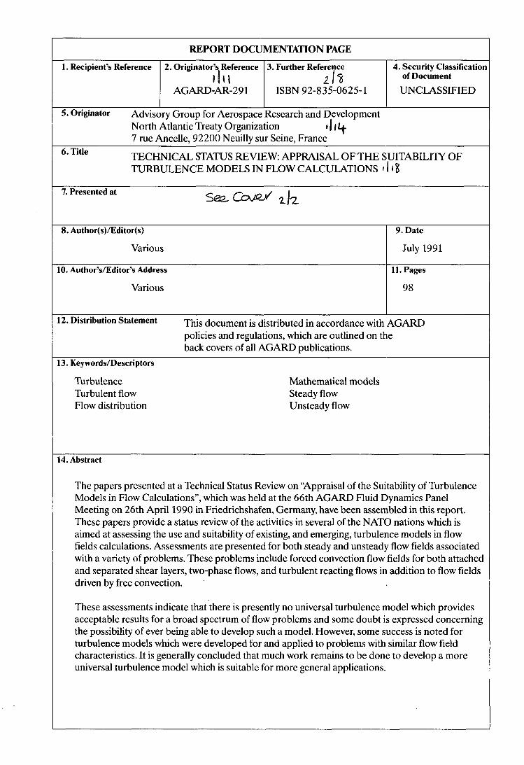
REPORT DOCUMENTATION PAGE

1. Recipient’s Reference 2. Originator’s Reference 3. Further Reference 4. Security Classificatior

AGARD-AR-291 ISBN 92-8 3 5-062 5-1 UNCLASSIFIED l l I l 21% of Document

TECHNICAL STATUS REVIEW APPRAISAL OF THE SUITABILITPI’ OF TURBULENCE MODELS IN FLOW CALCULATIONS 1 18

6. Title

8. Author(s)/Editor(s)

Various

LO. Author’dEditor’s Address

Various

7. Presented at

9. Date

July 1991

11. Pages

98

I

12. Distribution Statement This document is distributed in accordance with AGARD policies and regulations, which are outlined on the back covers of all AGARD publications.

13. Keywords/Descriptors

Turbulence Turbulent flow Flow distribution

Mathematical models Steady flow Unsteady flow

14. Abstract

The papers presented at a Technical Status Review on “Appraisal of the Suitability of Turbulence Models in Flow Calculations”, which was held at the 66th AGARD Fluid Dynamics Panel Meeting on 26th April 1990 in Friedrichshafen, Germany, have been assembled in this report. These papers provide a status review of the activities in several of the NATO nations which is aimed at assessing the use and suitability of existing, and emerging, turbulence models in flow fields calculations. Assessments are presented for both steady and unsteady flow fields associated with a variety of problems. These problems include forced convection flow fields for both attached and separated shear layers, two-phase flows, and turbulent reacting flows in addition to flow fields driven by free convection.

These assessments indicate that there is presently no universal turbulence model which provides acceptable results for a broad spectrum of flow problems and some doubt is expressed concerning the possibility of ever being able to develop such a model. However, some success is noted for turbulence models which were developed for and applied to problems with similar flow field characteristics. It is generally concluded that much work remains to be done to develop a more universal turbulence model which is suitable for more general applications.

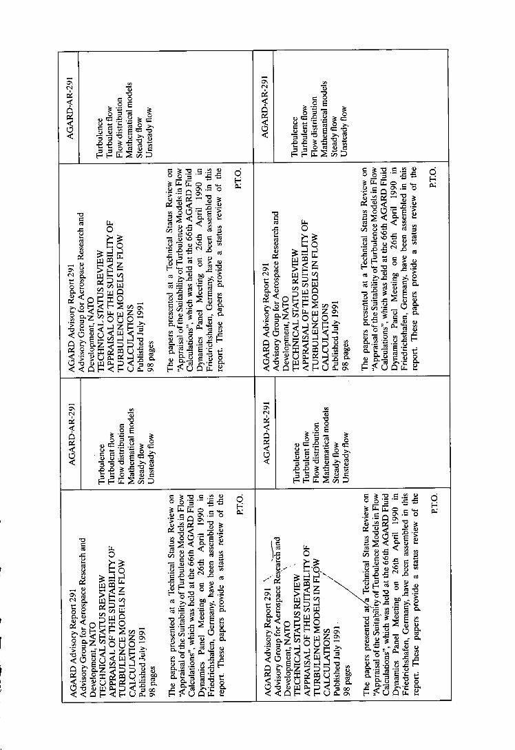
U C m L L

0

m 0 U

6

Y

c: c:

z \o

W w

0 m N

L

6 W z

0

c: m N

e

a@- NATO -@- OTAN

7 RUE ANCELLE * 922W NEUILLY-SUR-SEINE

FRANCE

DIFFUSION DES F'UBLICAIIONS AGARD NON CLAsSlFIEES

T6lhphone (1)47.38.57.00 * Tdax 610 176 TCldcopie (1)47.38.57.99

L'AGARD ne ditient as de stocks de sea publications, dans un but de distribution ghirale P l'adresse ddessus. La diffusion initiale des bticntions de I'AGA)RD est effeetUee auprk des pays membres de cette orgatusation par I'intermkliaire des Centres Nationaux de

!hibution suivants. Al'exception des Etais-Unis,ceacentresdispos?nt psrfoisd'eremplaires additionnels;dans Iescascontreire,on peut se procurer cea cxemplaires sow forme de microfiches ou de microcopies auprka dw Agencea de Vente don1 la lite suite.

CENTRES DE DIFFUSION NATIONAUX ALLEMAGNE ISLANDE

Fachinformationszentrum. Director of Aviation Karlsruhe c/o Flugrad D-7514 E ~ e n s t e i n - L e o p o I ~ e n 2 Reykjavilr

BELGIQUE Cwrdonnatew AGARD-VSL Etat-Major de la Force A6rieMe Quartier Reine Elisabetb Rue d'Evere, 1 140 BrweUes

CANADA Directew du .%vice des Rensei ements ScientBques Ministbre de la Efense Nation% Otmwa,OntarioKIAOKZ

DANEMARK DsnishDefenceRcaearchBoard Val ldraetsparken 4 2100 Copenhsgen 0

ETATS-UNIS National Aeronautics and Space Administration Langley Research Center ws 180 Hampton, Virginia 23665

FRANCE 0.NE.RA. $Dire+on) 29, Avenue e la h w o n Lcderc 92320. Ch&illon sous Bagneux

GRECE Hellenic Air Force Air War CoUe Scientific and b n i c a l Library Dekelia Air Force Base Dekelia,AthmTGA 1010

ITALIE Aeronautica Militaire Ufficio del Delegato Nazionale all'AGARD 3 Fiazzale Adcnauer 00144 Roma EUR

Voir Belgique

Nome$ian Defence m c h Establishment Am: Wblioteket P.O. Box 25 N-2W7 Kjeller

Netherlands Delegation to AGARD National Aerospace Laboratory NLR Kluyvenveg 1

LUXEMBOURG

NORVEGE

P4YSBAS

2629 HS Deut rORTUGAL

Portuguese National Coordinator to AGARD Gabinete de Estudos e Programs CLAFA Base de Alfragjde Alfragide 2700 M o r a

Defence Research Information Centre Kentigem House 65 Brown Street Glasgow 0 2 8EX

Mil11 Savunma Bapkanli& ARGE Daire Ba$mI@ ( RG ) Ankara

ROYAUME UN1

T U R Q F

!PS% LE CENTRE NATIONAL DE DISTRIBUTION DES ETATSUNIS (NASA NE DETENT PAS DE STOCKS

AU SERVICE NATIONAL TECHNIQUE DE L'INFORMATION (NTIS) DONT CADRESSE SUIT. DE.s p u B L i c A n ~ N s A G A m ET LEs DEMANDEs ~XEMPLNRES DOiVEllT E m mREssEES D i R E m M E m

National Tec41nial Wormation Service

E?ort Royal Road S ri eld,Virginia22161 2tasnis

AGENCES DE VENTE ESNInformation Retrieval Service European Space Agency IO. rue Mano Nikis 75(

Lesdemsodesdemicrofi~soudephotocopiesdedoc~entsAGARD~comprisIesdemaodesfaitwau duNTK3)doiventcomporter I a d t n o m i o s ( i w A G A R D . a i n s i q u e l e n u m c m d e ~ r i e d e l ' A G A R D ~ a r ~ ~ l ~ A G ~ A ~ 3 l ~ ~ o r m a t i o n s ~ ~ e s , t e l l w queleti~eetladatedepuhticationsontso~tables.VeuiUernoter U llyalieu espBclfierAGARD- wet AGARD-AR-nnnlordela commandede rapports AGARDet des rapportsconsultati~s A G A ~ r e s ~ t i v e m M r Dea r6fCrences bibliopphiquescomplhesainsique des riSumeS des publications AGARD figurent dans les joumux su~vantss:

Scienwque and Technical A e m ce Reports (STAR) puMi6 par la NASA Scientific >Technical Information Division $ri&ld

"H?yte"&W Washington C 205 Etats-Unis Etaw-Unis

Government Reports Announcements and Index (GRAM) uMi6 BT le National Technical Wormation Sernce

lrguua 22161

$cces,sible 6plement en mode interactif dans la base de onnees hbbographiques en time du NTIS, et sw CD-ROM)

Imprime par Specialived t inting Services Limited 40 C-11 Lune, Loughton, Esru IGlO 312

THE UNneD STATES NATIONAL STOCKS OF AOARD PUBLICATIONS,

DIRECTTOTHE NAllONAL TECHNICAL INFORMATON SERVICE

1 I 1 I

I I

1 I

i i 1 \

i 1

Documents

~praisal of the Suitability of - NATO STO