1

On Gaussian Half-Duplex Relay NetworksMartina Cardone, Daniela Tuninetti, Raymond Knopp and Umer Salim

Abstract—This paper considers Gaussian relay networks wherea source transmits a message to a sink terminal with the help ofone or more relay nodes. The relays work in half-duplex mode, inthe sense that they can not transmit and receive at the same time.For the case of one relay, the generalized Degrees-of-Freedomis characterized first and then it is shown that capacity canbe achieved to within a constant gap regardless of the actualvalue of the channel parameters. Different achievable schemesare presented with either deterministic or random switch for therelay node. It is shown that random switch in general achieveshigher rates than deterministic switch. For the case of K relays,it is shown that the generalized Degrees-of-Freedom can beobtained by solving a linear program and that capacity can beachieved to within a constant gap of K/2 log(4K). This gap maybe further decreased by considering more structured networkssuch as, for example, the diamond network.

Index Terms—Relay Channel, Generalized Degrees-of-Freedom, Capacity to within a Constant Gap, Inner bound,Outer bound, Half-duplex.

I. INTRODUCTION

The performance of wireless systems can be enhanced byenabling cooperation between the wireless nodes. The simplestform of cooperation is modeled by the Relay Channel (RC)where a source terminal communicates to a destination withthe help of a relay node. In this multi-hop system the relayhelps to increase the coverage and the throughput of thenetwork.

Relays employed in practical wireless networks can beclassified into two categories: Full-Duplex (FD) and Half-Duplex (HD). In the former case the relays transmit andreceive simultaneously; in the latter case the relays can eithertransmit or receive at any given time, but not both. There aresome relatively expensive relay devices which work in FDmode, normally used in military communications. HoweverFD relaying in wireless networks has practical restrictions such

M. Cardone and R. Knopp are with the Mobile CommunicationsDepartment at Eurecom, Sophia Antipolis, 06560, France (e-mail: car-done@eurecom.fr; knopp@eurecom.fr). D. Tuninetti is with the Electrical andComputer Engineering Department of the University of Illinois at Chicago,Chicago, IL 60607 USA (e-mail: danielat@uic.edu). U. Salim is with Al-gorithm Design group of Intel Mobile Communications, Sophia Antipolis,06560, France (e-mail: umer.salim@intel.com).

The work of D. Tuninetti was partially funded by NSF under award number0643954; the contents of this article are solely the responsibility of the authorand do not necessarily represent the official views of the NSF. The workof D. Tuninetti was possible thanks to the generous support of Telecom-ParisTech, Paris France, while the author was on a sabbatical leave at the sameinstitution. Eurecom’s research is partially supported by its industrial partners:BMW, Cisco Systems, Monaco Telecom, Orange, SFR, ST Ericsson, SAP,Swisscom and Symantech. The research work carried out at Intel by U. Salimhas received funding from the European Community’s Seventh FrameworkProgram (FP7/2007-2013) SACRA project (grant agreement number 249060)

The results in this paper have been submitted in part to the 2013 IEEEInternational Conference on Communications (ICC) and to the 2013 IEEEInternational Symposium on Information Theory (ISIT).

as self-interference, which make the implementation of decod-ing algorithm challenging. As a result HD relaying proves tobe a more practical technology with its relatively simple signalprocessing. Thus it is more realistic to assume that the relayoperates in HD mode either in Frequency Division Duplexing(FDD) or Time Division Duplexing (TDD). In FDD, therelay uses one frequency band to transmit and another oneto receive; in TDD, the relay listens for a fraction γ ∈ [0, 1]of time and then transmits in the remaining 1−γ time fraction.From an application point of view, the HD model fits future4G network with relays [1], where the relay communicatesover-the-air with the source, which is called the Donor-eNB.We keep our focus on deployment scenarios where the relayworks in TDD HD mode.

In this work we concentrate on the HD relay networks,where the relays transmit and receive in different time slots.HD relaying has received considerable attention lately, assummarized next.

A. Related Work

a) Single Relay Networks: The RC was first introducedby van der Meulen [2] and then thoroughly studied by Coverand El Gamal [3]. In [3] the authors study the general memo-ryless RC, derive inner and outer bounds on the capacity andestablish the capacity for some classes of RCs. The proposedouter bound is now known as the max-flow min-cut outerbound, or cut-set for short, which can be extended to moregeneral memoryless networks [4]. Two achievable relayingstrategies were proposed in [3], whose combination is stillthe largest known achievable rate for a general RC, namelyDecode-and-Forward (DF) and Compress-and-Forward (CF).In DF, the relay fully decodes the message sent by thesource and then coherently cooperates with the source tocommunicate this information to the destination. In CF, therelay does not attempt to recover the source message, but itjust compresses the information received and then sends it tothe destination. The capacity of the general memoryless RCis known for some special classes, in particular for degradedRCs, reversely degraded RCs and semi-deterministic RC [3].

The HD-RC was studied by Host-Madsen in [5]. Herethe author derives both an upper and a lower bound on thecapacity. The former is based on the cut-set arguments, thelatter exploits the Partial-Decode-and-Forward (PDF) strategywhere the relay only decodes part of the message sent by thesource. Host-Madsen considers the transmit/listen state of therelay as fixed and therefore known a priori to all nodes.

In [6], Kramer shows that larger rates can be achieved byusing a random transmit/listen switch strategy at the relay. Inthis way, the source and the relay can harness the randomnessthat lies in the switch in order to transmit extra information. An

arX

iv:1

301.

5522

v1 [

cs.I

T]

23

Jan

2013

2

important observation of [6] is that there is no need to developa separate theory for memoryless networks with HD nodes asthe HD constraints can be incorporated into the memorylessFD framework. In this work we shall adopt this approach inderiving outer and inner bounds for HD relay networks.

b) Multiple Relay Networks: The pioneering work ofCover and El Gamal [3] has been extended to networks withmultiple relays. In [7] Kramer et al. proposed several innerand outer bounds as a generalization of DF, CF and the cut-set bound. It was shown that DF achieves the ergodic capacityof a wireless Gaussian network with phase fading if phaseinformation is available only locally and the relays are closeto the source node.

The exact characterization of the capacity region of ageneral memoryless network is challenging. Recently it hasbeen advocated that progress can be made towards under-standing the capacity by showing that achievable strategiesare provably “close” to (easily computable) outer bounds [8].As an example, Etkin et al. characterized the capacity of theGaussian Interference Channel to within 1 bit regardless of thesystem parameters [9]. In [10], the authors study unicast andmulticast Gaussian relay networks with K nodes and show thatcapacity can be achieved to within

∑Kk=1 5 min{Mk, Nk} bits

with quantize-remap-and-forward (QMF), where Mk and Nkare the number of transmit and receive antennas, respectively,of node k ∈ [1 : K]. Interestingly, the result is valid for staticand ergodic fading networks where the nodes operate eitherin FD mode or in HD mode with deterministic listen/transmitschedule for the relays. For single antenna systems, Lim et al.in [11] recently showed that this 5K bits gap can be reducedto 0.6K bits for FD relay networks with noisy network coding(NNC). Both QMF and NNC are network extensions of CF.

The gap characterization of [11] is valid for any multi relaynetwork but linear in the number of nodes in the network,which could be a too coarse capacity characterization fornetworks with a large number of nodes. Tighter gaps canbe obtained for more structured networks. For example, thediamond network model was first proposed in [12]. A diamondnetwork consists of a source, a destination and K − 2 relays.The source and the destination cannot communicate directlyand the relays cannot communicate among themselves. Inother words, a general Gaussian multi relay network with Knodes is characterized by K(K − 1) channel gains, while adiamond network only has 2(K − 2) non zero channel gains.In [12] the case of two relays was studied for which an achiev-able region based on time sharing between DF and amplify-and-forward (AF) was proposed. The capacity of a general FDdiamond network is known to within 2 log(K − 1) bits [13].If in addition the FD diamond network is symmetric, that is,all source-relay links are equal and all relay-destination linksare equal, the gap is less than 2 bits for any K [14]. HDdiamond networks have been studied as well, albeit only fordeterministic switch for the relays. In a HD diamond networkwith (K − 2) relays, there are 2K−2 possible combinationsof listening and transmit states, since each relay can eithertransmit or receive. For the case of (K − 2) = 2 relays, [15]shows that out of 2K−2 = 4 possible states only (K − 1) = 3states suffice to achieve capacity to within less than 4 bits.

Their achievable scheme is a clever extension of the two-hopDF strategy of [16]. It is interesting to note that [15] derivedclosed-form expressions for the fractions of time the relays areactive and tight outer bounds based on the dual of the linearprogram (LP) associated with the classical cut-set bound.Extensions of these ideas to more than two relays appeardifficult due to the combinatorial structure of the problem.

Inspired by [15], the authors in [17] showed that for a veryspecific HD diamond network with (K−2) = 3 relays, (K−1) = 4 states out of 2K−2 = 8 are active in the cut-set outerbound. In the same work, it was verified numerically that for ageneral HD diamond network with (K−2) ≤ 7 relays, (K−1)states suffice for the cut-set upper bound and it is conjecturedthat the same holds for any number of relays. We remark thatin [17] only the cut-set upper bound was considered; moreoveronly the case of deterministic switch and per-symbol powerconstraint was considered.

Multi relay networks were also studied in [18] where theauthors determine numerically the optimal fractions of timeeach relay transmits/receives with DF through an iterativealgorithm. Also in this case the relays use deterministic switch.

B. Contributions

In this work we focus on the HD relay networks. The exactcapacity of this channel is unknown. In this paper we makeprogress toward determining its capacity by giving a constantgap result for any Gaussian network with random switch. Ourmain contribution can be summarized as follows:

1) We determine the generalized Degrees-of-Freedom(gDoF) of the HD RC with a single relay. We identifythree schemes that achieve the gDoF upper bound. Thesimplest one is inspired by the Linear DeterministicApproximation (LDA) of the Gaussian noise channelat high SNR [10]; it uses superposition coding at thesource, DF at the relay and stripping decoding at boththe relay and destination; we note that neither power al-location nor backward decoding is required at the nodes.The second and third schemes use more sophisticatedcoding techniques and are based on PDF and NNCstrategies [4].

2) We prove that the three schemes above achieve thecapacity to within a constant gap regardless of thechannel parameters. We consider both deterministic andrandom switch for the relay. Thus in the second case therelay harnesses the randomness that lies in the switch toachieve larger rates and therefore smaller gaps from thecut-set upper bound.

3) We prove that PDF with random switch is optimal fora Gaussian diamond network with one relay, i.e., itachieves the capacity, even though we were not ableto determine the capacity achieving input distribution.

4) We determine the capacity of the noiseless LDA channel.In particular we show that random switch and non-uniform inputs at the relay are optimal.

5) For HD networks with K nodes (HD-MRC), allof which employ random switch, we prove thatNNC achieves the cut-set outer bound to within

3

K/2 log(4K) bits. For diamond relay networks assum-ing that the conjecture in [17] holds for any K, the gapcan be reduced to 5 log(K).

C. Paper OrganizationThe rest of the paper is organized as follows. Section

II describes the channel model and states our main result.Section III derives the gDoF upper-bound based on the cut-set bound. Section IV provides a lower bound based on thePDF strategy. Section V highlights a motivating example basedon the LDA and provides a simple achievable based on thisapproach. Sections VI and VII are devoted to the analytical andnumerical proofs that the capacity for a single relay network isachievable to within a constant gap, respectively. Section VIIIconsiders networks with multiple relays and it shows that thegDoF can be computed by solving a linear program and thatNNC achieves the capacity to within a constant gap. SectionIX concludes the paper.

II. SINGLE RELAY NETWORKS: SYSTEM MODEL

A. General Memoryless Relay ChannelA RC consists of two input alphabets (Xs,Xr), two output

alphabets (Yr,Yd) and a transition probability PYr,Yd|Xs,Xr .The source sends symbols from Xs, the relay receives symbolsin Yr and sends symbols from Xr, and the destination receivessymbols in Yd. The source has a message W ∈ [1 : 2NR] forthe destination where N denotes the codeword length and Rthe transmission rate in bits per channel use 1. At time i,i ∈ [1 : N ], the source maps its message W into a channelinput symbol Xs,i(W ) and the relay maps its past channelobservations into a channel input symbol Xr,i(Y

i−1r ). The

channel is assumed to be memoryless, that is, the followingMarkov chain holds for all i ∈ [1 : N ]

(W,Y i−1r , Y i−1d , Xi−1s , Xi−1

r )→ (Xs,i, Xr,i)→ (Yr,i, Yd,i).

At time N , the destination makes an estimate W (Y Nd ) of themessage W based on all its channel observations Y Nd . A rateR is said to be ε-achievable if P[W 6= W ] ≤ ε for someε ∈ [0, 1]. The capacity is the largest nonnegative rate that isε-achievable for any ε > 0.

We note that half-duplex channels are a special case of thememoryless full-duplex framework in the following sense [6]:let the channel input of the relay be the pair (Xr, Sr), whereXr ∈ Xr as before and Sr ∈ {0, 1} is the state randomvariable that indicates whether the relay is in receive-mode(Sr = 0) or in transmit-mode (Sr = 1). The memorylesschannel transition probability is defined as

PYr,Yd|Xs,Xr,Sr=0 = P(0)Yr,Yd|Xs,Sr=0

PYr,Yd|Xs,Xr,Sr=1 = P(1)Yd|Xs,Xr,Sr=1P

(1)Yr|Sr=1,

that is, when the relay is in receive-mode (Sr = 0) theoutputs Yr, Yd are independent of Xr and when the relay is intransmit-mode (Sr = 1) the relay output Yr is independent ofeverything else. In other words, the (still memoryless) channelis now specified by the two transition probabilities one for eachmode of operation [6].

1Logarithms are in base 2.

B. The Gaussian Half-Duplex RC

We consider a single-antenna complex-valued GaussianHalf-Duplex Relay Channel (G-HD-RC), shown in Fig. 1,where the inputs are subject to an average power constraint,described by the input/output relationship

Yr =√CXs (1− Sr) + Zr, (1a)

Yd =√SXs + ejθ

√IXr Sr + Zd, θ ∈ R, (1b)

where the channel gains C, S, I are constant and thereforeknown to all terminals. Without loss of generality we canassume that the relay output Yr does not contain the relayinput Xr because the relay node can always subtract Xr

from Yr. Moreover, since a node can compensate for thephase of one of its channel gains, we can assume withoutloss of generality that the channel gains from the source tothe other two terminals are real-valued and nonnegative. Thechannel inputs are subject to unitary average power constraintswithout loss of generality, i.e., E[|Xu|2] ≤ 1, u ∈ {s, r}. The‘switch’ random variable Sr is binary. The noises Zd, Zr areassumed to be zero-mean jointly Gaussian and with unit powerwithout loss of generality. In particular (but not without lossof generality) in this work we assume that Zd is independentof Zr. In the following we will only consider G-HD-RC forwhich C > 0 and I > 0 in (2), since for either C = 0 orI = 0 the relay is disconnected from either the source or thedestination, respectively, so the channel reduces to a point-to-point channel with capacity log(1 + S).

The capacity of the channel in (1) is unknown. Here wemake progress toward determining its capacity by establishingits gDoF, i.e., an exact capacity characterization in the limitfor infinite SNR [9], and its capacity to within a constant gapat any finite SNR. Consider SNR > 0 and the parameterization

S := SNRβsd , source-destination link, (2a)

I := SNRβrd , relay-destination link, (2b)

C := SNRβsr , source-relay link, (2c)

for some (βsd, βrd, βsr) ∈ R3+. We define:

Definition 1. The gDoF is

d(HD−RC) := limSNR→+∞

C(HD−RC)

log(1 + SNR),

where C(HD−RC) is the capacity of the G-HD-RC.

Definition 2. The capacity C(HD−RC) is said to be known towithin b bits if one can show rates R(in) and R(out) such that

R(in) ≤ C(HD−RC) ≤ R(out) ≤ R(in) + b log(2).

Our main result for single relay networks can be summa-rized as

Theorem 1. The gDoF of the G-HD-RC is given by (3) at thetop of next page and the cut-set upper bound is achieved towithin the following number of bits

Achievable scheme LDA NNC PDFanalytical gap 3 1.61 1numerical gap 1.59 1.52 1

4

d(HD−RC) =

{βsd + (βrd−βsd)(βsr−βsd)

(βrd−βsd)+(βsr−βsd)for βsr > βsd, βrd > βsd

βsd otherwise.(3)

where LDA is a very simple achievable scheme inspired by thelinear deterministic approximation of the G-HD-RC at highSNR, PDF is partial-decode-and-forward and NNC is noisy-network-coding, or compress-and-forward.

Sections III-VII are devoted to the proof of Theorem 1.

Remark 1. The gDoF of the Gaussian Full-Duplex RelayChannel (G-FD-RC) is

d(FD−RC) = βsd + min{[βsr − βsd]+, [βrd − βsd]+}, (4)

and its capacity C(FD−RC) is achievable to within 1 bitper channel use [10]. We notice that HD achieves the samegDoF of FD if min{βrd, βsr} ≤ βsd, in which case the RCbehaves gDoF-wise like a point-to-point channel from TX toRX with gDoF given by βsd. In either FD or HD the gDoFhas a ‘routing’ interpretation [10]: if the weakest link fromthe source to the destination through the relay is smallerthan the direct link from the source to the destination thendirect transmission is optimal and the relay can be kept silent,otherwise it is optimal to communicate with the help of therelay.

III. SINGLE RELAY NETWORKS: UPPER BOUND

This section is devoted to the proof of a number of upperbounds that we shall use for the converse part of Theorem 1.From the cut-set bound we have:

Proposition 1. The capacity of the G-HD-RC is upperbounded as in (5), (6) and (7) at the top of next page where

• in (5): the distribution P ∗Xs,Xr,Sr is the one that maxi-mizes the cut-set upper bound,

• in (6): the parameter γ := P[Sr = 0] ∈ [0, 1] representsthe fraction of time the relay node listens, H(γ) is thebinary entropy function defined as

H(γ) := −γ log(γ)− (1− γ) log(1− γ), (12)

the maximization is over the set

γ ∈ [0, 1], (13)|α1| ≤ 1, (14)

(Ps,0, Ps,1, Pr,0, Pr,1) ∈ R4+

: γPu,0 + (1− γ)Pu,1 ≤ 1, u ∈ {s, r}, (15)

and the mutual informations I1, . . . , I4 are defined as

I1 := log (1 + S Ps,0) , (16)

I2 := log(

1+SPs,1+IPr,1+2|α1|√SPs,1IPr,1

), (17)

I3 := log (1 + (C + S)Ps,0) , (18)

I4 := log(1 + (1− |α1|2)S Ps,1

), (19)

• in (7): the terms b1 and b2 are defined as

b1 :=log(

1 + (√I +√S)2)

log (1 + S)> 1 since I > 0, (20)

b2 :=log (1 + C + S)

log (1 + S)> 1 since C > 0. (21)

Proof: The proof and the definitions of the above quan-tities can be found in Appendix A.

The upper bound in (5) will be used to prove that PDF withrandom switch achieves capacity to within 1 bit, the one in (6)to prove that PDF with deterministic switch also achievescapacity to within 1 bit and for numerical evaluations (sincewe do not know the distribution P ∗Xs,Xr,Sr that maximizes thecut-set upper bound in (5)), and the one in (7) for analyticalcomputations such as the derivation of the gDoF.

Proposition 2. The gDoF of the G-HD-RC is upper boundedby the right hand side of (3).

Proof: The proof can be found in Appendix B.

IV. SINGLE RELAY NETWORKS: LOWER BOUNDS BASEDON PARTIAL-DECODE-AND-FORWARD

This section is devoted to the proof of a number of lowerbounds that we shall use for the direct part of Theorem 1.From the achievable rate with PDF we have:

Proposition 3. The capacity of the G-HD-RC is lowerbounded as in (8), (9) and (10) at the top of next page where

• in (8): we fix the input PU,Xs,Xr,Sr to evaluate the PDFlower bound; in particular we set PXs,Xr,Sr to be thesame distribution that maximizes the cut-set upper boundin (5) and we choose either U = Xr or U = XrSr +Xs(1− Sr).

• in (9): the parameter γ := P[Sr = 0] ∈ [0, 1] representsthe fraction of time the relay node listens, the maximiza-tion is over the set (13)-(15) as for the cut-set upperbound in (6), the mutual informations I5, . . . , I8 are

I5 := I1 in (16), (22)I6 := I2 in (17), (23)I7 := log (1 + max{C, S}Ps,0) ≤ I3 in (18), (24)I8 := I4 in (19), (25)

and I(PDF)0 := I(Sr;Yd) is computed from the density

fYd(t)=γ

πv0exp(−|t|2/v0)+

1− γπv1

exp(−|t|2/v1),

(26)

with t ∈ C, v0 = exp(I5), v1 = exp(I6).

5

C(HD−RC) ≤ min{I(Xs, Xr, Sr;Yd), I(Xs;Yr, Yd|Xr, Sr)

}∣∣∣(Xs,Xr,Sr)∼P∗Xs,Xr,Sr

(5)

≤ max min{H(γ) + γI1 + (1− γ)I2, γI3 + (1− γ)I4

}=: r(CS−HD) (6)

≤ 2 log(2) + log (1 + S)

(1 +

(b1 − 1)(b2 − 1)

(b1 − 1) + (b2 − 1)

), (7)

C(HD−RC) ≥ min{I(Xs, Xr, Sr;Yd),

I(U ;Yr|Xr, Sr) + I(Xs;Yd|Xr, Sr, U)}∣∣∣

(Xs,Xr,Sr)∼P∗Xs,Xr,Sr and U = Xr or U = XrSr +Xs(1− Sr), (8)

C(HD−RC) ≥ max min{I(PDF)0 + γI5 + (1− γ)I6, γI7 + (1− γ)I8

}=: r(PDF−HD) (9)

≥ log (1 + S)

(1 +

(c1 − 1)(c2 − 1)

(c1 − 1) + (c2 − 1)

), (10)

r(LDA−HD) :=log(1 + S)+log(

1 + I1+S

)log(

1+ I1+S

)+[log(

1+ C1+S

)−log

(1+ S

1+S

)]+ [log

(1+

C

1 + S

)−log

(1+

S

1+S

)]+. (11)

• in (10): the terms c1 and c2 are

c1 :=log (1 + I + S)

log (1 + S)> 1 since I > 0, (27)

c2 :=log (1 + max{C, S})

log (1 + S)> 1 since C > 0. (28)

Proof: The proof can be found in Appendix C.The lower bound in (8) will be compared to the upper

bound in (5) to prove that PDF with random switch achievescapacity to within 1 bit, the one in (9) with the one in (6)to prove that PDF with deterministic switch also achievescapacity to within 1 bit and for numerical evaluations, andthe one in (10) for analytical computations such as evaluationof the achievable gDoF.

Proposition 4. The gDoF of the G-HD-RC is lower boundedby the right hand side of (3).

Proof: The proof can be found in Appendix D.Propositions 2 and 4 show that the gDoF for the G-HD-RC

is given by (3).

V. SINGLE RELAY NETWORKS: A SIMPLE ACHIEVABLESTRATEGY

In this section we propose a very simple achievable schemethat is gDoF optimal, that achieves capacity to within 3 bitsand that can be implemented in practical HD relay networks.In Section V-A we describe a deterministic-switch achievablestrategy for the Linear Deterministic Approximation (LDA) ofthe G-HD-RC at high SNR which we mimic in Section V-Bto derive an achievable rate for the G-HD-RC at any SNR.This achievable scheme is referred to as the LDA-strategy, orLDA for short. The main result of this section is:

Proposition 5. The capacity of the G-HD-RC is lowerbounded as in (11) at the top of this page.

The rest of the section is devoted to the proof of Proposi-tion 5. Before we provide the details of the scheme, we pointout three important practical aspects of this scheme that areworth noticing:

1) the destination does not use backward decoding, whichsimplifies the decoding procedure and incurs no delay,

2) the destination uses successive decoding, which is sim-pler than joint decoding, and

3) no power allocation is applied at the source or at therelay, which simplifies the encoding procedure and canbe used for time-varying channel as well. The sourceuses superposition coding to ‘route’ part of its datathrough the relay.

These aspects will be clear from the actual description of thescheme. Moreover we can show that

Proposition 6. The LDA strategy achieves the gDoF upperbound in (3).

Proof: The proof can be found in Appendix E.

A. A Motivating Example

The LDA of the G-HD-RC in (1) is a deterministic channelwith input-output relationship

Yr = Sn−βsrXs (1− Sr), (29a)

Yd = Sn−βsdXs + Sn−βrdXr Sr, (29b)

for some nonnegative integers βsr, βsd, βrd, where the inputsand outputs are vectors of length n := max{βsr, βsd, βrd} andS is the n× n shift matrix [10].

The capacity of a deterministic RC is given by the cut-setupper bound [10]. For the LDA in (29) the cut-set upper-boundevaluates to

6

C(HD) =

{βsd + maxγ∈[0,1] min

{(1− θ∗ (γ)) log 1

1−θ∗(γ) + θ∗ (γ) log L−1θ∗(γ) , γ[βsr − βsd]+

}for βsr > βsd, βrd > βsd

βsd otherwise.(30)

max{R} = maxPXs,Xr,Sr

min{I(Xs, Xr, Sr;Yd), I(Xs;Yr, Yd|Xr, Sr)

}= maxPXs,Xr,Sr

min{H(Yd), H(Yr, Yd|Xr, Sr)

}≤ maxPXs,Xr,Sr

min{H(Yd|Sr), H(Yr, Yd|Xr, Sr)

}+H(Sr)

≤ maxγ∈[0,1]

min{γβsd + (1− γ) max{βsd, βrd}, γmax{βsd, βsr}+ (1− γ)βsd}+ log(2)

= βsd + γ∗LDA[βsr − βsd]+ + log(2), (31)

Theorem 2. The capacity of the deterministic HD RC in (29)is given by (30) at the top of this page where θ∗ (γ) = 1 −max{1/L, γ} and L := 2[βrd−βsd]

+

.

Proof: The proof can be found in Appendix K.Next we further upper bound the capacity in (30) because

our goal is to get insights into asymptotically optimal strategiesfor the G-HD-RC. For the channel in (29) we have that (31)at the top of this page holds, where γ∗LDA is the optimal γ :=P[Sr = 0] ∈ [0, 1] obtained by equating the two argumentswithin the min and is given by

γ∗LDA :=

{(βrd−βsd)

(βrd−βsd)+(βsr−βsd)for βrd > βsd, βsr > βsd

0 otherwise.

Next we show that the upper bound in (31) is achievableto within log(2) = 1 bit. This 1 bit represents the maximumamount of information I(Sr;Yd) that could be conveyed tothe destination by a random switch at the relay. If we neglectthe term log(2) we can achieve the upper bound in (31)with the scheme shown in Figs. 2(a) and 2(b) for the casemin{βsr, βrd} > βsd, which is the case where the upperbound differs from direct transmission, i.e., Xr = 0. InPhase I/Fig. 2(a) the relay listens and the source sends b1 (oflength βsd bits) directly to the destination and b2 (of lengthβsr − βsd bits) to the relay; note that b2 is below the noisefloor at the destination; the duration of Phase I is γ, hencethe relay has accumulated γ(βsr − βsd) bits to forward to thedestination. In Phase II/Fig. 2(b) the relay forwards the bitslearnt in Phase I to the destination by ‘repackaging’ them intoa (of length βrd − βsd bits); the source keeps sending a newb1 (of length βsd bits) directly to the destination; note that adoes not interfere at the destination with b2; the duration ofPhase II is such that all the bits accumulated in Phase I canbe delivered to the destination, that is

γ(βsr − βsd) = (1− γ)(βrd − βsd),

which gives precisely the optimal γ∗LDA. The total number ofbits decoded at the destination is

1 · βsd + γ∗LDA · (βsr − βsd),

which gives precisely the optimal gDoF for the half-duplexchannel in (3).

Remark 2. The HD optimal strategy in Figs. 2(a) and 2(b)should be compared with the FD optimal strategy in Fig. 2(c).In Fig. 2(c), in a given time slot t, the source sends b1[t] (oflength βsd bits) directly to the destination and b2[t + 1] (oflength at most βsr − βsd bits) to the relay; the relay decodesboth b1[t] and b2[t+1] and forwards b2[t+1] in the next slot;in slot t the relay sends b2[t] (of length at most βrd − βsdbits) to the destination; the number of bits the relay forwardsmust be the minimum among the number of bits the relaycan decode (given by βsr − βsd) and the number of bits thatcan be decoded at the destination without harming the directtransmission from the source (given by βrd − βsd). Therefore,the total number of bits decoded at the destination is

βsd + min{βrd − βsd, βsr − βsd},

which gives precisely the optimal gDoF for the full-duplexchannel in (4)

Remark 3. Fig. 3 compares the capacities of the FD and HDLDA channels; it also shows some achievable rates for the HDLDA channel. In particular, the capacity of the FD channel isgiven by (4) (dotted black curve labeled “FD”), the capacityof the HD channel is given by (30) (solid black curve labeled“HD” obtained with the optimal p∗0 in Appendix K) and itsupper bound by (31) (red curve labeled “HDlda upper”). Forcomparison we also show the performance when the sourceuses i.i.d. Bernoulli(1/2) bits and the relay uses one of thefollowing strategies: i.i.d. Bernoulli(q) bits and random switch(blue curve labeled “HDiid q+rand” obtained by numericallyoptimizing q ∈ [0, 1]), i.i.d. Bernoulli(1/2) bits and randomswitch (green curve labeled “HDiid 1/2+rand” obtained withp0 = 1/L in Appendix K), and i.i.d. Bernoulli(1/2) bits anddeterministic switch (magenta curve labeled “HDiid 1/2+det”and given by βsd + min{γ[βsr−βsd]+, (1− γ)[βrd−βsd]+}).We can draw conclusions from Fig. 3:• With deterministic switch: i.i.d. Bernoulli(1/2) bits for

the relay are optimal but this choice is quite far fromcapacity (magenta curve vs. solid black curve); thischoice however is at most one bit from optimal (magentacurve vs. red curve).

• With random switch: the optimal input distribution for therelay is not i.i.d. bits; i.i.d. inputs incurs a rate loss (blue

7

curve vs. solid black curve); if in addition we insist oni.i.d. Bernoulli(1/2) bits for the relay we incur a furtherloss (green curve vs. blue curve).

This shows that for optimal performance the relay inputs arecorrelated and that random switch should be used.

B. An achievable strategy inspired by the LDA

We can mimic the LDA strategy in Section V-A for the G-HD-RC as follows. We assume S < C, otherwise we use directtransmission to achieve R = log(1 + S). The transmission isdivided into two phases:• Phase I of duration γ: the transmit signals are

Xs[1] =√

1− δXb1[1] +√δXb2 , δ =

1

1 + S,

Xr[1] = 0.

The relay applies successive decoding of Xb1[1] followedby Xb2 from

Yr[1] =√C√

1− δXb1[1] +√C√δXb2 + Zr[1],

which is possible if (rates are normalized by the totalduration of the two phases)

Rb1[1] ≤ γ log (1 + C)− γ log

(1 + C

1

1 + S

)Rb2 ≤ γ log

(1 + C

1

1 + S

). (32)

The destination decodes Xb1[1] treating Xb2 as noise from

Yd[1] =√S√

1− δXb1[1] +√S√δXb2 + Zd[1],

which is possible if

Rb1[1] ≤ γ log (1 + S)− γ log

(1 + S

1

1 + S

). (33)

Finally, since we assume S < C, Phase I is successfulif (32) and (33) are satisfied.

• Phase II of duration 1− γ: the transmit signals are

Xs[2] = Xb1[2]

Xr[2] = Xb2

The destination applies successive decoding of Xb2 (byexploiting also the information about b2 that it gatheredin the first phase) followed by Xb1[2] from

Yd[2] =√SXb1[2] + e+jθ

√IXb2 + Zd[2],

which is possible if

Rb2≤ (1−γ) log

(1+

I

1+S

)+γ log

(1+

S

1+S

)(34)

Rb1[2] ≤ (1− γ) log(1 + S). (35)

• By imposing that the rate Rb2 is the same in both phases,that is, that (32) and (34) are equal, we get that γ shoulddue chosen equal to γ∗

γ∗=log(

1 + I1+S

)log(

1 + I1+S

)+log

(1 + C

1+S

)−log

(1 + S

1+S

) .

Note that γ∗ → γ∗LDA as SNR increases. Moreoverwe give here an explicit closed form expression for theoptimal duration of the time the relay listens to thechannel.The rate sent directly from the source to the destination,that is, the sum of (33) and (35), is

Rb1[1] +Rb1[2] = log(1 + S)− γ∗ log

(1 +

S

1 + S

)︸ ︷︷ ︸

∈[0,log(2)]

.

Therefore the total rate decoded at the destination throughthe two phases is

Rb1[1] +Rb1[2] +Rb2 = r(LDA−HD) in (11).

We notice that the rate expression for r(LDA−HD) in (11),which was derived under the assumption C > S, is validfor all C since for C < S it reduces to direct transmissionfrom the source to the destination.

VI. SINGLE RELAY NETWORKS: ANALYTICAL GAPS

In the previous sections we described upper and lowerbounds to determine the gDoF of the G-HD-RC. Here weshow that the same upper and lower bounds are to within aconstant gap of one another thereby concluding the proof ofTheorem 1. We consider both the case of random switch andof deterministic switch for the relay.

Proposition 7. [PDF and random switch] PDF with randomswitch is optimal to within 1 bit.

Proof: The proof can be found in Appendix G.

Proposition 8. [PDF and deterministic switch] PDF withdeterministic switch is optimal to within 1 bit.

Proof: The proof can be found in Appendix H.

Proposition 9. [LDA (deterministic switch)] LDA is optimalto within 3 bits.

Proof: The proof can be found in Appendix I.

We conclude this section with a discussion on the gap thatcan be obtained with NNC. The NNC strategy is a networkgeneralization of the CF. It has been proposed for generalmemoryless networks and it is optimal to within a constant gapfor full-duplex multicast networks with an arbitrary numberof relays, where the gap grows linearly with the number ofrelays [11]. In the case with only one relay, NNC reducesto the classical CF [4, Remark 18.6] and represents a goodalternative to the PDF especially in the case when the linkbetween the source and the relay is weaker than the directlink. The NNC rate is presented in Appendix F. By usingRemark 5 in Appendix F we have

Proposition 10. [NNC and deterministic switch] NNC withdeterministic switch is optimal to within 1.61 bits.

Proof: The proof can be found in Appendix J.

8

VII. SINGLE RELAY NETWORKS: NUMERICAL GAPS

In this section we show that the gap results obtained inSection VI are pessimistic and are due to crude bounding inboth the upper and lower bounds, which was necessary in orderto obtain rate expressions that could be handled analytically. Inorder to illustrate our point, we first consider a relay networkwithout the source-destination link, that is, with S = 0, inSection VII-A and then we show that the same observationsare valid for any network in Section VII-B.

A. Single Relay Networks without a Source-Destination Link,a.k.a. Diamond Networks with One Relay

c) Upper Bound: We start by showing that the (upperbound on the) cut-set upper bound in (6) can be improvedupon. Note that we were not able to evaluate the actual cut-set upper bound in (5) so we further bounded it as in (6),which for S = 0 reduces to

r(CS−HD)|S=0 = maxγ∈[0,1]

min

{H(γ)+(1−γ) log

(1+

I

1−γ

),

γ log

(1 +

C

γ

)}.

The capacity of the G-FD-RC for S = 0 is known exactly andis given by the cut-set upper bound

C(FD)|S=0 = log (1 + min{C, I}) .

C(FD) is a trivial upper bound for the capacity of the G-HD-RC. Now we show that our upper bound r(CS−HD)|S=0 canbe larger than C(FD)|S=0. For the case C = 15/2 > I = 3/2we have

r(CS−HD)|S=0≥min

{H(

1

2

)+

1

2log (1+2I) ,

1

2log (1+2C)

}= log(4) > C(FD)|S=0 = log (2.5) .

The reason why the capacity of the FD channel can besmaller than our upper bound r(CS−HD)|S=0 is the crudebound I(Sr;Yd) ≤ H(Sr) = H(γ). As mentioned earlier, weneeded this bound in order to have an analytical expression forthe upper bound. Actually for S = 0 the cut-set upper boundin (5) is tight, as we show next.

d) Exact capacity with PDF:

Theorem 3. In absence of direct link between the source andthe destination PDF with random switch achieves the cut-setupper bound.

Proof: With S = 0, the cut-set upper bound in (5) and thePDF lower bound in (8) are the same (see also Appendix Gwith S = 0).

e) Improved gap for the LDA Lower Bound: Despiteknowing the capacity expression for S = 0, its actual eval-uation is elusive as it is not clear what the optimal inputdistribution P ∗Xs,Xr,Sr in (5) is. For this reason we nextspecialized the LDA strategy to the case S = 0 and evaluateits gap from the (upper bound on the) cut-set upper boundin (6).

The LDA achievable rate in (11) with S = 0 is given by

r(LDA−HD)|S=0 = maxγ∈[0,1]

min{γ log (1 + C)

(1− γ) log (1 + I)}.

and its gap from the outer bound can be reduced from 3 bitsto about 1.5 bits since

GAP ≤ r(CS−HD)|S=0 − r(LDA−HD)|S=0

≤ maxγ∈[0,1]

{γ log

(1 +

C

γ

)− γ log (1 + C) ,

H(γ)+(1− γ) log

(1+

I

1−γ

)−(1−γ) log (1+I)

}≤ maxγ∈[0,1]

{γ log

(1

γ

),H(γ) + (1− γ) log

(1

1− γ

)}= maxγ∈[0,1]

{H(γ)+(1− γ) log

(1

1−γ

)}=1.5112 bits.

Note that the actual gap is even less than 1.5 bits.By numerically evaluating the difference betweenmin{C(FD), r(CS−HD)}|S=0 and r(LDA−HD)|S=0 we foundthat the gap is at most 1.11 bits.

f) Numerical gaps with deterministic switch: Similarly,by numerical evaluations one can find that the PDF strat-egy with deterministic switch in Remark 4-Appendix C andthe NNC strategy with deterministic switch in Remark 5-Appendix F are to within 0.80 bits and 1.01 bits, respectively,of the improved upper bound. Notice that in these cases thereis no information conveyed by the relay to the destinationthrough the switch. Further reductions in the gap with randomswitch are discussed next for a general network.

Fig. 4 shows different upper an lower bounds for the G-HD-RC for S = 0, C = 15, I = 3 vs γ = P[Sr = 0].We see that the cut-set upper bound exceeds the capacityof the G-FD-RC (maximum of the solid black curve vs.dashed black curve). Different achievable strategies are alsoshown, whose order from the most performing to the leastperforming is: PDF with random switch (red curve, 1.913bits/ch.use), PDF with deterministic switch (blue curve, 1.702bits/ch.use), NNC with random switch (cyan curve, 1.446bits/ch.use), NNC with deterministic switch (magenta curve,1.402 bits/ch.use), and LDA (green curve, 1.333 bits/ch.use).In this particular setting, the maximum rate using the NNCstrategy with random switch (cyan curve, 1.446 bits/ch.use)is achieved for P[Q = 0, Sr = 0] = 0,P[Q = 0, Sr = 1] =0.33,P[Q = 1, Sr = 0] = 0.45,P[Q = 1, Sr = 1] = 0.22.This is due to the absence of the direct link (S = 0) betweenthe source and the destination. Actually, since the source cancommunicate with the destination only through the relay, itis necessary a coordination between the transmissions of thesource and those of the relay. This coordination is possiblethanks to the time-sharing random variable Q, i.e. when Q = 0the source stays silent, while when Q = 1 the source transmits.

B. Single Relay Network with a Source-Destination Link

Although the considerations in Section VII-A were for arelay channel without a source-destination link, they are validin general.

9

Fig. 5 and Fig. 6 show the rates achieved by using thedifferent achievable schemes presented in the previous sectionswith S > 0. In Fig. 5 the channel conditions are such thatthe PDF strategy outperforms the NNC, while in Fig. 6 theopposite holds. In Fig. 5 the PDF strategy with random switch(red curve, 11.66 bits/ch.use) outperforms both the NNCwith random switch (cyan curve, 11.11 bits/ch.use) and thePDF with deterministic switch (blue curve, 11.4 bits/ch.use);then the PDF with deterministic switch outperforms the NNCwith deterministic switch (magenta curve, 10.94 bits/ch.use),which is also encompassed by the NNC with random switch.Differently from the case without direct link, we observe thatthe maximum NNC rates both in Fig. 5 and in Fig. 6 areachieved with the choice Q = ∅, i.e. the time-sharing randomvariable Q is a constant. This is due to the fact that thesource is always heard by the destination even when the relaytransmits so there is no need for the source to remain silentwhen the relay sends.

In Fig. 7 we consider the case of deterministic switch. Fig. 7shows, as a function of SNR for βsd = 1, (βrd, βsr) ∈ [0, 2.4],the maximum gap between the cut-set upper bound r(CS−HD)

in (6) and the following lower bounds with deterministicswitch: the PDF lower bound obtained from r(PDF−HD) in (9)with I

(PDF)0 = 0, the NNC lower bound in Remark 5 in

Appendix F, and the LDA lower bound in (11). From Fig. 7we observe that the maximum gap with PDF is of 1 bit asin Proposition 8, but with NNC is around 1.52 bits and withLDA is around 1.59 bits, which are lower than the analyticalgaps we found in Propositions 10 and 9, respectively.

The lower bounds can be improved upon by consideringthat information can be transmitted through a random switchfor the relay. However, this improvement depends on thechannel gains. If the information cannot be routed throughthe relay because min{C, I} ≤ S, then the system cannotexploit the randomness of the switch, and so IPDF

0 = 0 andINNC0 = 0 are approximately optimal (in this case the relay

can remain silent). For this reason the maximum numericalgap obtained with a random switch coincides with the oneobtained with a deterministic switch, as there are channelconditions for which random switch is not necessary. Thisbehavior for the PDF strategy is represented in Fig. 8. Inthis figure we numerically evaluate the difference between theanalytical gap, i.e., the one computed with IPDF

0 = 0, andthe numerical one, i.e., computed with Iopt0 (actual value ofIPDF0 ), at a fix SNR = 20dB and by varying (βrd, βsr). We

observe that when the information cannot be conveyed throughthe relay, i.e., min {βrd, βsr} ≤ 1, then IPDF

0 = 0 is optimal,since the information only flows through the direct link. InFig. 9 the channel channel gains are set such that the use ofthe relay increases the gDoF of the channel (βsd = 1 and(βrd, βsr) ∈ [1, 2.4]). Here the relay uses PDF. We observethat we have a further improvement in terms of gap by usinga random switch (blue curve) instead of using a deterministicswitch (red curve). We notice that at high SNR, where thegap is maximum, this improvement is around 0.1 bits. Asmentioned earlier, the rate advantage of random switch overdeterministic switch depends on the channel gains.

VIII. NETWORKS WITH MULTIPLE RELAYS

In this section we extend our gDoF and gap results togeneral HD-MRC. Similarly to the the full-duplex case [11],our main result is that NNC is optimal to within a constant gapfor the HD-MRC where the gap is a function of the numberof relays.

A. Network Model

In this model we have K ≥ 3 nodes, i.e., one transmit-ter/node 1, one receiver/node K and K−2 relays with indices2, . . . ,K − 1. Each node is equipped with a single antennaand is subject to an average power constraint, which we setto 1 without loss of generality, i.e. E

[|Xk|2

]≤ 1 ∈ R+,

k ∈ [1 : K − 1]. The system is described by the input/outputrelationship

Y = (I− S)HS X + Z (36a)

Z = [Z1, . . . , ZK ]T ∼ N (0, I) (36b)

Y = [Y1, . . . , YK ]T ∈ CK (36c)

X = [X1, . . . , XK ]T ∈ CK :

E[|Xk|2] ≤ 1 for k ∈ [1 : K − 1], (36d)

H ∈ CK×K (36e)S = diag{S1, . . . , SK} :

S1 = 1, Sk ∈ {0, 1} for k ∈ [2 : K − 1], SK = 0, (36f)

where the vector S represents the state of the nodes, eitherreceive (S = 0) or transmit (S = 1). The channel matrixH ∈ CK×K is constant and therefore known to all terminals.The entry hij with (i, j) ∈ [1 : K]2 represents the channelbetween source j and destination i. Without loss of generalitywe assume that the noises Z are zero-mean jointly Gaussianand with unit power. Furthermore we assume that the noisesare iid N (0, 1), this is however not without loss of general-ity [19].

The capacity of the channel described in (36) is not knownin general. Here we show that a scheme based on the NNCstrategy achieves the capacity within a constant gap for anynumber of relays and for any choice of channel parameters.As for the FD case, the gap is found to be a function of thenumber of relays. We propose a different and simpler boundingtechnique than that of [11], which might overestimate theactual gap between inner and outer bound.

B. Capacity to within a constant gap

Our main result is

Theorem 4. The cut-set upper bound for the half-duplex multi-relay network is achievable to within

GAP ≤ max`∈[0:K−2]

{min{1 + `,K − 1− `} log (1 + `)

+ min{1 + 3`, `+K − 1}} (37)

bits per channel use.

Proof: The proof can be found in Appendix L.

10

For high value of K, i.e. K >> 1, the optimal value of `in (37) is ` ∼= K−2

2 and the corresponding limit gap becomes

GAP ∼=K

2log(4K). (38)

Fig. 10 shows the trend of the gap in (37) as a function of thenumber of nodes K (blue curve). The red curve represents thelimit behaviour of the gap in (37).

Note that by applying the above gap-result to the case K =3 we obtain GAP ≤ 4 bits which is a much larger gap than1.61 bits we found for the case of one relay.

A smaller gap may be obtained by computing tighterbounds. This can be accomplished by several means. Forexample:

• By using more complex and sophisticated bounding tech-niques: in [11] an upper bound on the water-filling powerallocation for a general MIMO channel was derived. Thismore involved upper bound could be used here to obtain asmaller gap. We note that our bounding technique appliedto the FD-MRC gives a gap of order K

2 log(2K), whichis larger that 0.63K found in [11].

• By using an achievable strategy based on PDF, which in asingle relay case gives a smaller gap than NNC. However,PDF seems not to be easily extended to networks with anarbitrary number of relays, which is the main motivationwe consider NNC here.

• By deriving tighter bounds on specific network topolo-gies: in [20] it is found that for a FD diamond networkwith K relays the gap is of the order log(K), rather thanlinear in K [11]. Moreover, for a symmetric FD diamondnetwork with K relays the gap does not depend on thenumber of relays and is upper bounded by 2 bits. Thekey difference between a general multi-relay network anda diamond network is that for each subset A we haveRank[HA,s] = 2, i.e., the rank of a generic channel sub-matrix does no longer depend on the cardinality of A.Based on this observation we haveProposition 11. The cut-set upper bound for the gaussianhalf-duplex diamond network with (K − 2) relays isachievable to within

GAP ≤ (K − 2) log(2) + 4 log(K) + 2 log(e/2).

Moreover, if the conjecture in [17] holds then the gapabove could be decreased to

GAP ≤ 5 log(K) + 2 log(e/2).

Proof: The proof can be found in Appendix M.

C. Example: Fully connected network with K = 4

To gain insights into how relays are best utilized, weconsider a network with two relays, i.e. K = 4 nodes. Inparticular we highlight under which channel conditions thegDoF performance is enhanced by exploiting both relays ratherthan using only the best one. We also compare the loss thatincurs by using HD with respect to FD. Let parameterize the

channel gains as

[log(|hij |2)

log(SNR)

](i,j)∈[1:4]2

=

∗ ∗ ∗ ∗αs1 ∗ β1 ∗αs2 β2 ∗ ∗1 α1d α2d ∗

where ∗ denotes entries that do not matter; this is so becausethe source node never listens to the channel (first row), thedestination node never transmits (last column), and a relaycan remove the ‘self-interference’ (main diagonal). Note thatthe direct link from the source to the destination has gain SNRand all other channel gains are expressed with reference to it.

g) Full Duplex: In the following the set A indicates therelays that lie on the source/node 1 side of the cut. The cut-setupper bound for the FD-MRC [11] gives

A = ∅ : I1 := I(X1;Y4, Y2, Y3|X2, X3)

≤ log(1 + |h41|2 + |h21|2 + |h31|2)

A = {2} : I2 := I(X1, X2;Y4, Y3|X3)

≤ log |I2 + H1HH1 |+ log(2)

= log (1 +A) + 2 log(2)

A = {3} : I3 := I(X1, X3;Y4, Y2|X2)

≤ log |I2 + H2HH2 |+ log(2)

= log (1 +B) + 2 log(2)

A = {2, 3} : I4 := I(X1, X2, X3;Y4|∅)≤ log(1 + (|h41|+ |h42|+ |h43|)2),

where

A = |h41|2 + |h42|2 + |h31|2 + |h32|2 + |h31h42 − h32h41|2,B = |h41|2 + |h43|2 + |h21|2 + |h23|2 + |h21h43 − h23h41|2,

I2 =

[1 00 1

], H1 =

[h31 h32h41 h42

]and H2 =

[h21 h23h41 h43

].

Thus for the full-duplex case, the cut-set bound is given by

r(CS−FD) := min {I1, I2, I3, I4}

which at high SNR gives the following gDoF (achievable towithin a constant gap [11])

d(FD)K=4 = lim

SNR→+∞

r(CS−FD)

log(1 + SNR)

= min{

max {1, αs1, αs2} ,max {αs2 + α1d, β2 + 1} ,

max {αs1 + α2d, β1 + 1} ,max {1, α1d, α2d}}.

In the following we are interested in identifying cases forwhich

d(FD)K=4 > d

(FD)K=4,best relay := max

{1,min{αs1, α1d},min{αs2, α2d}

},

where d(FD)K=4,best relay is the gDoF that can be obtained by

selecting the relay which achieves the highest gDoF in (4)while leaving the other silent. From the expression for d

(FD)K=4

11

we immediately see that in order to have d(FD)K=4 > 1, i.e., better

than direct transmission with the two relays silent, we need

max {αs1, αs2} > 1,

max {αs2 + α1d − 1, β2} > 0,

max {αs1 + α2d − 1, β1} > 0,

max {α1d, α2d} > 1.

We therefore distinguish the following cases:1) if αs1 > max{1, αs2} and α1d > max{1, α2d} then

d(FD)K=4 = min{αs1, α1d} = d

(FD)K=4,best relay > 1;

therefore this case is not interesting;2) if αs1 > max{1, αs2} and α2d > max{1, α1d} then

d(FD)K=4 = min

{αs1,max {αs2 + α1d, β2 + 1} , α2d

}.

Next consider the following sub-cases:a) If α1d ≤ 1 or αs2 ≤ 1, then d

(FD)K=4,best relay < d

(FD)K=4,

hence in this case using both relays can give anunbounded rate improvement over using the bestrelay if max {αs2 + α1d − 1, β2} > 0;

b) If α1d > 1 and αs2 > 1, then d(FD)K=4,best relay =

max{

min{αs1, α1d},min{αs2, α2d}}> 1; we

distinguishi) If αs1 ≤ α1d or α2d ≤ αs2 then

d(FD)K=4,best relay = min{αs1, α2d} = d

(FD)K=4,

therefore this case is not interesting;ii) If αs1 > α1d and α2d > αs2 then

d(FD)K=4,best relay = max{α1d, αs2} < d

(FD)K=4,

therefore we have a strict improvement byusing both relays over using only the best relay.

3) Considering cases similar to the two above but with therole of the relays swapped complete the list of possiblecases.

An example of network satisfying the conditions in item 2aor item 2(b)ii is given in Fig. 11 where the numerical valueon a link represents the SNR exponent on the correspondinglink.

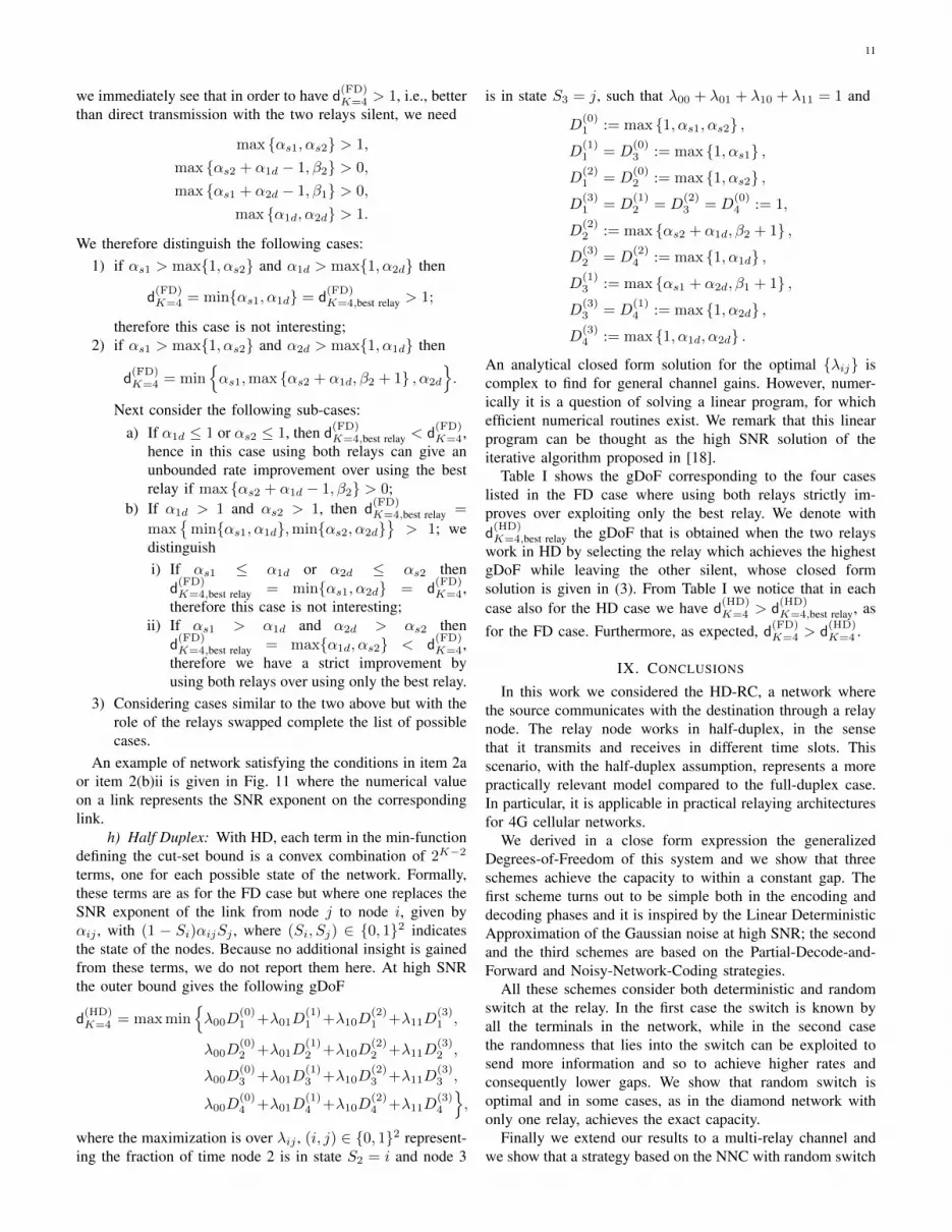
h) Half Duplex: With HD, each term in the min-functiondefining the cut-set bound is a convex combination of 2K−2

terms, one for each possible state of the network. Formally,these terms are as for the FD case but where one replaces theSNR exponent of the link from node j to node i, given byαij , with (1 − Si)αijSj , where (Si, Sj) ∈ {0, 1}2 indicatesthe state of the nodes. Because no additional insight is gainedfrom these terms, we do not report them here. At high SNRthe outer bound gives the following gDoF

d(HD)K=4 = max min

{λ00D

(0)1 +λ01D

(1)1 +λ10D

(2)1 +λ11D

(3)1 ,

λ00D(0)2 +λ01D

(1)2 +λ10D

(2)2 +λ11D

(3)2 ,

λ00D(0)3 +λ01D

(1)3 +λ10D

(2)3 +λ11D

(3)3 ,

λ00D(0)4 +λ01D

(1)4 +λ10D

(2)4 +λ11D

(3)4

},

where the maximization is over λij , (i, j) ∈ {0, 1}2 represent-ing the fraction of time node 2 is in state S2 = i and node 3

is in state S3 = j, such that λ00 + λ01 + λ10 + λ11 = 1 and

D(0)1 := max {1, αs1, αs2} ,

D(1)1 = D

(0)3 := max {1, αs1} ,

D(2)1 = D

(0)2 := max {1, αs2} ,

D(3)1 = D

(1)2 = D

(2)3 = D

(0)4 := 1,

D(2)2 := max {αs2 + α1d, β2 + 1} ,

D(3)2 = D

(2)4 := max {1, α1d} ,

D(1)3 := max {αs1 + α2d, β1 + 1} ,

D(3)3 = D

(1)4 := max {1, α2d} ,

D(3)4 := max {1, α1d, α2d} .

An analytical closed form solution for the optimal {λij} iscomplex to find for general channel gains. However, numer-ically it is a question of solving a linear program, for whichefficient numerical routines exist. We remark that this linearprogram can be thought as the high SNR solution of theiterative algorithm proposed in [18].

Table I shows the gDoF corresponding to the four caseslisted in the FD case where using both relays strictly im-proves over exploiting only the best relay. We denote withd(HD)K=4,best relay the gDoF that is obtained when the two relays

work in HD by selecting the relay which achieves the highestgDoF while leaving the other silent, whose closed formsolution is given in (3). From Table I we notice that in eachcase also for the HD case we have d

(HD)K=4 > d

(HD)K=4,best relay, as

for the FD case. Furthermore, as expected, d(FD)K=4 > d

(HD)K=4 .

IX. CONCLUSIONS

In this work we considered the HD-RC, a network wherethe source communicates with the destination through a relaynode. The relay node works in half-duplex, in the sensethat it transmits and receives in different time slots. Thisscenario, with the half-duplex assumption, represents a morepractically relevant model compared to the full-duplex case.In particular, it is applicable in practical relaying architecturesfor 4G cellular networks.

We derived in a close form expression the generalizedDegrees-of-Freedom of this system and we show that threeschemes achieve the capacity to within a constant gap. Thefirst scheme turns out to be simple both in the encoding anddecoding phases and it is inspired by the Linear DeterministicApproximation of the Gaussian noise at high SNR; the secondand the third schemes are based on the Partial-Decode-and-Forward and Noisy-Network-Coding strategies.

All these schemes consider both deterministic and randomswitch at the relay. In the first case the switch is known byall the terminals in the network, while in the second casethe randomness that lies into the switch can be exploited tosend more information and so to achieve higher rates andconsequently lower gaps. We show that random switch isoptimal and in some cases, as in the diamond network withonly one relay, achieves the exact capacity.

Finally we extend our results to a multi-relay channel andwe show that a strategy based on the NNC with random switch

12

TABLE I: gDoF when using both relays is better than using only the best one

Channel Parameters Full-duplex Full-duplex Half-duplex Half-duplex(αs1, αs2, α1d, α2d, β1, β2) best relay both relays best relay both relays

(2.5, 1.4, 0.5, 1.8, 0.6, 0.8) 1.4 1.8 1.267 1.4235(2.5, 0.3, 0.7, 1.3, 0.4, 0.8) 1.0 1.3 1.000 1.2182(1.8, 1.2, 1.3, 2.0, 0.7, 1.2) 1.3 1.8 1.218 1.5808(1.7, 1.1, 1.2, 1.4, 0.4, 1.5) 1.2 1.4 1.156 1.3604

at each relay, achieves the capacity to within a constant gap.We also prove that this gap may be even decreased in morestructured settings as, for example, the diamond network wherethere are no source-destination and relay-relay links.

REFERENCES

[1] LTE-A, 3rd Generation Partnership Project; Technical SpecificationGroup Radio Access Network; Evolved Universal Terrestrial RadioAccess (EUTRA), 3GPP TR 36.806 V9.0.0, 2010.

[2] E. C. van der Meulen, “Three-terminal communication channel,” Adv.Appl. Probab., vol. 3, pp. 120–154, 1971.

[3] T. Cover and A.E. Gamal, “Capacity theorems for the relay channel,”IEEE Trans. on Info. Theory, vol. 25, no. 5, pp. 572 – 584, Sep. 1979.

[4] Abbas El Gamal and Young-Han Kim, Network Information Theory,Cambridge Univ. Press,, Cambridge U.K., 2011.

[5] A. Host-Madsen, “On the capacity of wireless relaying,” in VehicularTechnology Conference, 2002. Proceedings. VTC 2002-Fall. 2002 IEEE56th, 2002, vol. 3, pp. 1333 – 1337 vol.3.

[6] Gerhard Kramer, “Models and theory for relay channels with receiveconstraints,” in in 42nd Annual Allerton Conf. on Commun., Control,and Computing, 2004, pp. 1312–1321.

[7] G. Kramer, M. Gastpar, and P. Gupta, “Cooperative strategies andcapacity theorems for relay networks,” Information Theory, IEEETransactions on, vol. 51, no. 9, pp. 3037 – 3063, sept. 2005.

[8] Amir Salman Avestimehr, Wireless network information flow: a de-terministic approach, Ph.D. thesis, EECS Department, University ofCalifornia, Berkeley, Oct 2008.

[9] R.H. Etkin, D.N.C. Tse, and Hua Wang, “Gaussian interference channelcapacity to within one bit,” IEEE Trans. on Info. Theory, vol. 54, no.12, pp. 5534 –5562, Dec. 2008.

[10] A.S. Avestimehr, S.N. Diggavi, and D.N.C. Tse, “Wireless networkinformation flow: A deterministic approach,” Information Theory, IEEETransactions on, vol. 57, no. 4, pp. 1872 –1905, april 2011.

[11] Sung Hoon Lim, Young-Han Kim, A. El Gamal, and Sae-Young Chung,“Noisy network coding,” Information Theory, IEEE Transactions on,vol. 57, no. 5, pp. 3132 –3152, may 2011.

[12] B. Schein and R. Gallager, “The gaussian parallel relay network,” inInformation Theory, 2000. Proceedings. IEEE International Symposiumon, 2000, p. 22.

[13] Bobbie Chern and Ayfer Ozgur, “Achieving the capacity of the n-relaygaussian diamond network within log n bits,” CoRR, vol. abs/1207.5660,2012.

[14] U. Niesen and S. Diggavi, “Approximate capacity of the gaussian n-relay diamond network,” Information Theory, IEEE Transactions on,vol. PP, no. 99, pp. 1, 2012.

[15] H. Bagheri, A.S. Motahari, and A.K. Khandani, “On the capacity ofthe half-duplex diamond channel,” in Information Theory Proceedings(ISIT), 2010 IEEE International Symposium on, june 2010, pp. 649 –653.

[16] Feng Xue and S. Sandhu, “Cooperation in a half-duplex gaussiandiamond relay channel,” Information Theory, IEEE Transactions on,vol. 53, no. 10, pp. 3806 –3814, oct. 2007.

[17] S. Brahma, A. Ozgur, and C. Fragouli, “Simple schedules for half-duplex networks,” in Information Theory Proceedings (ISIT), 2012 IEEEInternational Symposium on, july 2012, pp. 1112 –1116.

[18] L. Ong, M. Motani, and S. J. Johnson, “On capacity and optimalscheduling for the half-duplex multiple-relay channel,” InformationTheory, IEEE Transactions on, vol. 58, no. 9, pp. 5770 –5784, sept.2012.

[19] Lili Zhang, Jinhua Jiang, A.J. Goldsmith, and Shuguang Cui, “Study ofgaussian relay channels with correlated noises,” Communications, IEEETransactions on, vol. 59, no. 3, pp. 863 –876, march 2011.

[20] Bobbie Chern and Ayfer Ozgur, “Achieving the capacity of the n-relaygaussian diamond network within log(n) bits,” IEEE Information TheoryWorkshop (ITW) 2012, Lausanne Switzerland (also arXiv:1207.5660),Sept. 2012.

APPENDIX APROOF OF PROPOSITION 1

Proof: An outer bound to the capacity of the memorylessRC is given by the cut-set outer bound [4, Thm.16.1] thatspecialized to our G-HD-RC channel gives

C(HD−RC)

≤ maxPXs,[Xr,Sr ]

min{I(Xs, [Xr, Sr];Yd), I(Xs;Yr, Yd|[Xr, Sr])

}(39a)

= maxPXs,Xr,Sr

min{I(Sr;Yd) + I(Xs, Xr;Yd|Sr),

I(Xs;Yr, Yd|Xr, Sr)}

(39b)

≤ maxPXs,Xr,Sr

min{H(Sr) + I(Xs, Xr;Yd|Sr),

I(Xs;Yr, Yd|Xr, Sr)}

(39c)

≤ max min{H(γ) + γI1 + (1− γ)I2, γI3 + (1− γ)I4

}=: r(CS−HD), (39d)

where the different steps follow since:• We indicate the (unknown) distribution that maxi-

mizes (39a) as P ∗Xs,Xr,Sr in order to get the bound in (5).• In order to obtain the bound in (39c) we used the fact

that for a discrete binary-valued random variable Sr wehave

I(Sr;Yd) = H(Sr)−H(Sr|Yd) ≤ H(Sr) = H(γ)

for some γ := P[Sr = 0] ∈ [0, 1] that represents thefraction of time the relay listens and where H(γ) is thebinary entropy function in (12). In (39d) the maximizationis over the set defined by (13)-(15) and is obtained as anapplication of the ‘Gaussian maximizes entropy’ principleas follows. Given any input distribution PXs,Xr,Sr , thecovariance matrix of (Xs, Xr) conditioned on Sr can bewritten as

Cov

[Xs

Xr

]∣∣∣∣Sr=`

=

[Ps,` α`

√Ps,`Pr,`

α∗`√Ps,`Pr,` Pr,`

],

with |α`| ≤ 1 for some (Ps,0, Ps,1, Pr,0, Pr,1) ∈ R4+ sat-

isfying the average power constraint in (15). Then, a zero-mean jointly Gaussian input with the above covariance

13

matrix maximizes the different mutual information termsin (39c). In particular

I(Xs, Xr;Yd|Sr = 0) ≤ log (1 + SPs,0) =: I1,

I(Xs, Xr;Yd|Sr = 1)

≤ log(

1+SPs,1+IPr,1+2|α1|√SPs,1 IPr,1

)=: I2,

I(Xs;Yr, Yd|Xr, Sr = 0)

≤ log(1 + (C + S)(1− |α0|2)Ps,0

)≤ log (1 + (C + S)Ps,0) =: I3,

I(Xs;Yr, Yd|Xr, Sr = 1) ≤ log(1 + S(1− |α1|2)Ps,1

)=: I4,

as defined in (16)-(19) thereby proving the upper boundin (6), which is the same as r(CS−HD) in (39d). Thisshows the bound in (6).

• In order to get to (7) from (6) we let the channel gains beparameterized as in (2). The average power constraints atthe source and at the relay given in (15) can be expressedas follows. Since the source transmits in both phases wedefine for some β ∈ [0, 1]

Ps,0 =β

γ,

Ps,1 =1− β1− γ

.

On the other hand, the relay transmission only affectsthe destination output for a fraction (1− γ) of the time,i.e., when Sr = 1, hence the relay must exploit all itsavailable power when Sr = 1; we therefore let

Pr,0 = 0,

Pr,1 =1

1− γ.

With this, the cut-set upper bound r(CS−HD) in (39d)can be rewritten as (40) at the top of next page where wedefined b1 and b2 as in (20)-(21), namely

b1 :=log(

1 + (√I +√S)2)

log (1 + S)> 1 since I > 0,

b2 :=log (1 + C + S)

log (1 + S)> 1 since C > 0.

Note that the optimal γ is found by equating the twoarguments of the max min and is given by

γ∗CS :=(b1 − 1)

(b1 − 1) + (b2 − 1).

This proves the upper bound in (7).

APPENDIX BPROOF OF PROPOSITION 2

Proof: The upper bound in (7) implies

d(HD−RC)

≤ limSNR→+∞

log (1 + S)

log (1 + SNR)

(1 +

(b1 − 1)(b2 − 1)

(b1 − 1) + (b2 − 1)

)= βsd

(1 +

[βrd/βsd − 1]+ [βsr/βsd − 1]+

[βrd/βsd − 1]+ + [βsr/βsd − 1]+

)= βsd +

[βrd − βsd]+ [βsr − βsd]+

[βrd − βsd]+ + [βsr − βsd]+,

since b1 → max{βsd, βrd}/βsd and b2 → max{βsd, βsr}/βsdat high SNR, which is equivalent to the right hand side of (3)after straightforward manipulations.

APPENDIX CPROOF OF PROPOSITION 3

The largest achievable rate for the memoryless relay channelis the combination of PDF and CF/NNC proposed in theseminal work of Cover and ElGamal [3]. Here we use PDF.The bound in (9) follows since:

Proof: The PDF scheme in [4, Thm.16.3] adapted to theHD model gives the following rate lower bound

C(HD−RC)

≥ maxPU,Xs,Xr,Sr

min{I(Sr;Yd) + I(Xs, Xr;Yd|Sr),

I(U ;Yr|Xr, Sr) + I(Xs;Yd|U,Xr, Sr)}

≥ max min{I(PDF)0 + γI5 + (1− γ)I6, γI7 + (1− γ)I8

}= r(PDF−HD) in (9),

where for the last inequality we let γ := P[Sr = 0] ∈ [0, 1]be the fraction of time the relay listens and, conditioned onSr = `, ` ∈ {0, 1}, we consider the following jointly Gaussianinput

UXs√Ps,`Xr√Pr,`

∣∣∣∣∣∣∣∣Sr=`

∼ N

0,

1 ρt|` ρr|`ρ∗t|` 1 α`ρ∗r|` α∗` 1

:

1 ρt|` ρr|`ρ∗t|` 1 α`ρ∗r|` α∗` 1

� 0.

In particular, we use specific values for the parameters{ρt|`, ρr|`, α`}`∈{0,1}, namely

∠α1 + θ = 0, (41a)

α0 = 0 and either |ρt|0|2 = 1− |ρr|0|2 = 0

or |ρr|0|2 = 1− |ρt|0|2 = 0, (41b)ρt|1 = α∗1, ρr|1 = 1. (41c)

14

r(CS−HD) = max(γ,|α1|,β)∈[0,1]3

min{H(γ) + γ log

(1 +

Sβ

γ

)+ (1− γ) log

(1 +

I

1− γ+S(1− β)

1− γ+ 2|α1|

√I

1− γS(1− β)

1− γ

),

0 + γ log

(1 +

Cβ

γ+Sβ

γ

)+ (1− γ) log

(1 + (1− |α1|2)

S(1− β)

1− γ

)}

≤ maxγ∈[0,1]

min{H(γ) + γ log

(1 +

S

γ

)+ (1− γ) log

1 +

(√I

1− γ+

√S

1− γ

)2 ,

0 + γ log

(1 +

C

γ+S

γ

)+ (1− γ) log

(1 +

S

1− γ

)}= maxγ∈[0,1]

min{

2H(γ) + γ log (γ + S) + (1− γ) log

(1− γ +

(√I +√S)2)

,

H(γ) + γ log (γ + C + S) + (1− γ) log (1− γ + S)}

≤ 2 log(2) + maxγ∈[0,1]

min{γ log (1 + S) + (1− γ) log

(1 +

(√I +√S)2)

, γ log (1 + C + S) + (1− γ) log (1 + S)}

= 2 log(2) + log (1 + S) maxγ∈[0,1]

min {γ + (1− γ)b1, γb2 + (1− γ)}

= 2 log(2) + log (1 + S)

(1 + max

γ∈[0,1]min {(1− γ)(b1 − 1), γ(b2 − 1)}

)= 2 log(2) + log (1 + S)

(1 +

(b1 − 1)(b2 − 1)

(b1 − 1) + (b2 − 1)

), (40)

With these definitions, the mutual information termsI(PDF)0 , I5, . . . , I8 in (9) are

I(Xs, Xr;Yd|Sr = 0) = log (1 + SPs,0) =: I5;

I(Xs, Xr;Yd|Sr = 1)

= log(

1 + SPs,1 + IPr,1 + 2|α1|√SPs,1 IPr,1

)=: I6,

(note I5 = I1 and I6 = I2 because of the assumption in (41a));next, by using the assumption in (41b), that is, in state Sr = 0the inputs Xs and Xr are independent, and that either U = Xs

or U = Xr, we have: if U = Xs independent of Xr

I(U ;Yr|Xr, Sr = 0) + I(Xs;Yd|U,Xr, Sr = 0) =

= I(Xs;√CXs + Zr|Xr, Sr = 0)

+ I(Xs;√SXs + Zd|Xs, Xr, Sr = 0)

= log (1 + CPs,0) + 0,

and if U = Xr independent of Xs

I(U ;Yr|Xr, Sr = 0) + I(Xs;Yd|U,Xr, Sr = 0) =

= I(Xr;√CXs + Zr|Xr, Sr = 0)

+ I(Xs;√SXs + Zd|Xr, Sr = 0)

= 0 + log (1 + SPs,0) ;

therefore under the assumption in (41b) we have

I(U ;Yr|Xr, Sr = 0) + I(Xs;Yd|U,Xr, Sr = 0)

= log (1 + max{C, S}Ps,0) =: I7;

next, by using the assumption in (41c), that is, in state Sr = 1

we let U = Xr, we have

I(U ;Yr|Xr, Sr = 1) + I(Xs;Yd|U,Xr, Sr = 1)

= I(Xr;Zr|Xr, Sr = 1) + I(Xs;√SXs + Zd|Xr, Sr = 1)

= 0 + I(Xs;√SXs + Zd|Xr, Sr = 1)

= log(1 + S(1− |α1|2)Ps,1

)=: I8,

(note I7 ≤ I3 and I8 = I4); finally

I(Sr;Yd)

= E[log

1

fYd(Yd)

]−[γ log(v0)+(1− γ) log(v1) + log(πe)]

=: I(PDF)0 ,

where fYd(·) is the density of the destination output Yd, whichis a mixture of (proper complex) Gaussian random variables,i.e.,

fYd(t) =γ

πv0exp(−|t|2/v0) +

1− γπv1

exp(−|t|2/v1), t ∈ C,

v0 := Var[Yd|Sr = 0] = exp(I5),

v1 := Var[Yd|Sr = 1] = exp(I6).

Note that I(PDF)0 = I(Sr;Yd) ≤ H(Sr) = H(γ). This proves

the lower bound in (9).Next we show how to further lower bound the rate in (9)

to obtain the rate expression in (10). With the same parame-

15

r(PDF−HD) = maxγ∈[0,1],|α|≤1,β∈[0,1]

min{I(PDF)0 + γ log

(1 +

βS

γ

)+(1− γ) log

(1 +

S(1− β)

1− γ+

I

1− γ+ 2|α|

√S(1− β)

1− γI

1− γ

),

γ log

(1 +

1

γmax {Cβ, Sβ}

)+ (1− γ) log

(1 + (1− |α|2)

S(1− β)

1− γ

)}≥ maxγ∈[0,1],β∈[0,1]

min

{0 + γ log

(1 +

βS

γ

)+ (1− γ) log

(1 +

S(1− β)

(1− γ)+

I

1− γ

),

γ log

(1 +

1

γmax {βC, βS}

)+ (1− γ) log

(1 +

S(1− β)

(1− γ)

)}≥ maxγ∈[0,1]

min {γ log (1 + S) + (1− γ) log (1 + S + I) , γ log (1 + max {C, S}) + (1− γ) log (1 + S)}

= log (1 + S) maxγ∈[0,1]

min {γ + (1− γ)c1, γc2 + (1− γ)}

= log (1 + S)

(1 + max

γ∈[0,1]min {(1− γ)(c1 − 1), γ(c2 − 1)}

)= log (1 + S)

(1 +

(c1 − 1)(c2 − 1)

(c1 − 1) + (c2 − 1)

), (42)

terization of the powers as in Appendix A, namely

Ps,0 =β

γ,

Ps,1 =1− β1− γ

,

Pr,0 = 0,

Pr,1 =1

1− γ.

we have (42) at the top of this page where we defined c1 andc2 as in (27)-(28), namely

c1 :=log (1 + I + S)

log (1 + S)≥ 1 since I > 0,

c2 :=log (1 + max{C, S})

log (1 + S)≥ 1 since C > 0.

Notice that ci ≤ bi, i = 1, 2, where bi, i = 1, 2, are definedin (20)-(21). The optimal γ, indicated by γ∗PDF is given by

γ∗PDF :=(c1 − 1)

(c1 − 1) + (c2 − 1)∈ [0, 1].

Remark 4. A further lower bound on the PDF rater(PDF−HD) in (9) can be obtained by trivially lower boundingI(PDF)0 ≥ 0, which corresponds to a fixed transmit/receive

schedule for the relay.

APPENDIX DPROOF OF PROPOSITION 4

Proof: The lower bound in (10) implies

d(HD−RC)≥ limS→+∞

log (1 + S)

log (1+SNR)

(1 +

(c1 − 1)(c2 − 1)

(c1 − 1) + (c2 − 1)

)= βsd

(1 +

[βrd/βsd − 1]+ [βsr/βsd − 1]+

[βrd/βsd − 1]+ + [βsr/βsd − 1]+

)= βsd +

[βrd − βsd]+ [βsr − βsd]+

[βrd − βsd]+ + [βsr − βsd]+,

since c1 → max{βsd, βrd}/βsd and c2 → max{βsd, βsr}/βsdat high SNR, which is equivalent to the right hand side of (3)after straightforward manipulations.

APPENDIX EPROOF OF PROPOSITION 6

Proof: The rate in (11) can be further lower bounded as

r(LDA−HD)≥− log(2)+log (1+S)

(1+

(c3−1)(c4−1)

(c3−1) + (c4−1)

),

where c3 := c1 = log(1+I+S)log(1+S) and c4 := b2 = log(1+C+S)

log(1+S) . Therate above implies

d ≥ limS→+∞

log (1 + S)

log (1 + SNR)

(1 +

(c3 − 1)(c4 − 1)

(c3 − 1) + (c4 − 1)

)= βsd

(1 +

[βrd/βsd − 1]+ [βsr/βsd − 1]+

[βrd/βsd − 1]+ + [βsr/βsd − 1]+

)= βsd +

[βrd − βsd]+ [βsr − βsd]+

[βrd − βsd]+ + [βsr − βsd]+,

since c3 → max{βsd, βrd}/βsd and c4 → max{βsd, βsr}/βsdat high SNR, which is equivalent to the right hand side of (3)after straightforward manipulations.

16

C(HD−RC) ≥ maxPQPXs|QP[Xr,Sr ]|QPYr|[Xr,Sr ],Yr,Q:|Q|≤2

min{I(Xs; Yr, Yd|[Xr, Sr], Q),

I(Xs, [Xr, Sr];Yd|Q)− I(Yr; Yr|Xs, [Xr, Sr], Yd, Q)}

= maxPQPSr|QPXs|QPXr|Sr,QPYr|Xr,Yr,Sr,Q:|Q|≤2

min{I(Xs; Yr, Yd|Q,Sr, Xr),

I(Sr;Yd|Q) + I(Xs, Xr;Yd|Sr, Q)− I(Yr; Yr|Xs, Xr, Yd, Sr, Q)}

≥ r(NNC−HD) in (44a), (43)

APPENDIX FACHIEVABLE RATE WITH NNC

The largest achievable rate for the memoryless relay channelis the combination of PDF and CF/NNC proposed in theseminal work of Cover and ElGamal [3]. Here we use NNCto show:

Proposition 12. The capacity of the G-HD-RC is lowerbounded as

C(HD−RC) ≥ r(NNC−HD)

:= max min{I(NNC)0 +

∑(i,j)∈[0:1]2

γijI9,ij ,∑

(i,j)∈[0:1]2γijI10,ij

},

(44a)

where the maximization is over

γij ∈ [0, 1] :∑

(i,j)∈[0:1]2γij = 1, (44b)

Ps,i ≥ 0 :∑

(i,j)∈[0:1]2γij Ps,i ≤ 1, (44c)

Pr,ij ≥ 0 :∑

(i,j)∈[0:1]2γij Pr,ij ≤ 1, (44d)

where the different mutual information terms in (44) aredefined next.

Proof: The NNC scheme in [4, Remark 18.5] adapted tothe HD model gives the rate lower bound in (43) at the top ofthis page, where the mutual information terms {I9,ij , I10,ij},(i, j) ∈ [0 : 1]2 and I(NNC)

0 in (44a) are obtained as follows.We consider the following assignment on the inputs and onthe auxiliary random variables for each (i, j) ∈ [0 : 1]2

P[Q = i, Sr = j] = γij such that (44b) is satisfied,(Xs

Xr

)∣∣∣∣Q=i,Sr=j

∼ N(

0,

[Ps,i 00 Pr,ij

])such that (44c) and (44d) are satisfied,

Yr|Xr,Yr,Q=i,Sr=j = Yr + Zr,ij ,

Zr,ij ∼ N (0, σ2ij) and independent of everything else,

and in order to meet the constraint that Xs cannot depend onSr conditioned on Q we must impose the constraint that instate Q = i, Sr = j the power of the source only depends on

the index i. Then for each (i, j) ∈ [0 : 1]2

I(Xs; Yr, Yd|Xr, Q = i, Sr = j)

= log

(1 +

(S +

C(1− j)1 + σ2

ij

)Ps,i

)=: I10,ij , (45)

I(Xs, Xr;Yd|Q = i, Sr = j)+

− I(Yr; Yr|Xs, Xr, Yd, Q = i, Sr = j)

= log (1+SPs,i+IjPr,ij)−log

(1+

1

σ2ij

)=: I9,ij , (46)

I(Sr;Yd|Q) = −∑(i,j)

γij log(vij)− log(πe)

+ (γ00 + γ01) E[log

1

f0(Y )|Q = 0

]+ (γ10 + γ11) E

[log

1

f1(Y )|Q = 1

]=: I

(NNC)0

Yd|Q=0 ∼ f0(t) :=γ00

γ00 + γ01

1

πv00exp(−|t|2/v00)

+γ01

γ00 + γ01

1

πv01exp(−|t|2/v01), t ∈ C,

Yd|Q=1 ∼ f1(t) :=γ10

γ10 + γ11

1

πv10exp(−|t|2/v10)

+γ11

γ10 + γ11

1

πv11exp(−|t|2/v11), t ∈ C,

vij := Var[Yd|Q = i, Sr = j] = 1 + S Ps,i + I j Pr,ij .

This proves the lower bound in (44) as a function ofσ2ij , (i, j) ∈ {0, 1}2.In order to find the optimal σ2

ij , (i, j) ∈ {0, 1}2 we reasonas follows. I10,ij in (45) is decreasing in σ2

ij while I9,ij in(46) is increasing. At the optimal point these two rates are thesame. Let

Ci := 1 +CPs,i

1 + SPs,i,

xi :=1

σ2i0

,

I ′ := I(Sr, Xr;Yd|Q),

and rewrite the lower bound in (44) as

r(NNC−HD) = (γ00 + γ01) log(1 + SPs,0)

+ (γ10 + γ11) log(1 + SPs,1)

− γ00 log (1 + x0)− γ10 log (1 + x1)

+ min{γ00 log (1+x0C0) + γ10 log (1+x1C1) , I ′

}.

17

The solution of

min(x0,x1)∈R2

+

{γ00 log (1 + x0) + γ10 log (1 + x1)

}subject to γ00 log (1 + x0C0) + γ10 log (1 + x1C1) = I ′

can be found to be

xi =[ηCi − 1]+

(1− η)Ci, i ∈ {1, 2},

with η ≤ 1 such that

γ00 log (1 + x0C0) + γ10 log (1 + x1C1) = I ′.

Remark 5. For the special case of Q = Sr, that is,I(NNC)0 = I(Sr;Yd|Q) = I(Q;Yd|Q) = 0, the achievable

rate in Proposition 12 reduces to

r(NNC−HD) ≥ max(γ,β)∈[0,1]2

min{γI9 + (1− γ)I10,

γI11 + (1− γ)I12

}, (48a)

I9 := log (1 + SPs,0)− log

(1 +

1

σ20

), (48b)

I10 := log (1 + SPs,1 + IPr,1) , (48c)

I11 := log

(1 + SPs,0 +

C

1 + σ20

Ps,0

)(48d)

I12 := log (1 + SPs,1) . (48e)

σ20 :=

B + 1

(1 +A)1γ−1 − 1

, (48f)

A :=IPr,1

1 + SPs,1, B :=

CPs,01 + SPs,0

, (48g)

Ps,0 =β

γ, Ps,1 =

1− β1− γ

, Pr,1 =1

1− γ, (48h)

where the optimal value for σ20 in (48f) is obtained by

equating the two expressions within the min in (48a).

Proposition 13. NNC with deterministic switch achieves thegDoF upper bound in (3).

Proof: With the achievable rate in Remark 5 (where herewe explicitly write the optimization wrt σ2

0) we have (47) atthe top of next page, where we defined c5 and c6 as

c5 = c1 :=log (1 + I + S)

log (1 + S)≥ 1 since I > 0 and as in (27),

c6 :=log(

1 + C1+σ2

0+ S

)log (1 + S)

≥ 1 since C > 0,

and where

γ∗NNC :=(c5 − 1)

(c5 − 1) + (c6 − 1)∈ [0, 1].

By reasoning as for the PDF in Appendix D, it follows fromthe last rate bound that NNC also achieves the gDoF in (3).

Remark 6. For the special case of Q = ∅, i.e., the time-sharing variable Q is a constant, the achievable rate inProposition 12 reduces to

r(NNC−HD) ≥ maxPXsPXr,SrPYr|[Xr,Sr ],Yr

min{I(Xs; Yr, Yd|Sr, Xr

),

I (Xs, Xr, Sr;Yd)−I(Yr; Yr|Sr, Xr, Xs, Yd

)}≥ maxγ∈[0,1],σ2

min

{γ log

(1+S+

C

1 + σ2

)+(1−γ) log (1+S) ,

I (Sr;Yd) + γ log (1 + S)− γ log

(1 +

1

σ2

)+(1− γ) log

(1 + S +

I

1− γ

)}.

Note that with Q = ∅ the source always transmits withconstant power, regardless of the state of the relay, whilethe relay sends only when in transmitting mode. Thus in thisparticular setting there is no coordination between the sourceand the relay.

APPENDIX GPROOF OF PROPOSITION 7

Proof: Consider the upper bound in (5) and the lowerbound in (8). Since the term I(Xs, Xr, Sr;Yd) is the same inthe upper and lower bound, the gap is given by2

GAP ≤I(Xs;Yr, Yd|Xr, Sr)− I(U ;Yr|Xr, Sr)

− I(Xs;Yd|Xr, Sr, U)

Next we consider two different choices for U :

• For C ≤ S we choose U = Xr and

GAP ≤ I(Xs;Yr, Yd|Xr, Sr)− I(Xs;Yd|Xr, Sr)

= I(Xs;Yr|Xr, Sr, Yd)

=P[Sr=0]I(Xs;√CXs+Zr|Xr, Sr=0,

√SXs+Zd)

+ P[Sr = 1]I(Xs;Zr|Xr, Sr = 1,√SXs + Zd)

≤ P[Sr = 0] I(Xs;√CXs + Zr|

√SXs + Zd)

≤ P[Sr = 0] log(1 + C/(1 + S))

≤ log(1 + S/(1 + S))

≤ log(2).

2 Let a lower bound be minA{fl(A)} and an upper bound beminA{fu(A)}. With the definition

Au,min := argminA{fu(A)}, Al,min := argmin

A{fl(A)},

we have fu(Au,min) ≤ fu(Al,min). This fact implies that the gap is upperbounded as

GAP ≤ minA{fu(A)} −min

A{fl(A)} = fu(Au,min)− fl(Al,min)

≤ fu(Al,min)− fl(Al,min) ≤ maxA{fu(A)− fl(A)}.

18

r(NNC−HD) ≥ maxγ∈[0,1],σ2

0≥0,β∈[0,1]min

{γ log

(1 +

βS

γ

)− γ log

(1 +

1

σ20

)+

+(1− γ) log

(1 +

(1− β)S

1− γ+

I

1− γ

),

γ log

(1 +

Cβ

(1 + σ20)γ

+Sβ

γ

)+ (1− γ) log

(1 +

(1− β)S

1− γ

)}β=γ

≥ maxγ∈[0,1],σ2

0≥0min {γ log (1 + S) + (1− γ) log (1 + S + I) ,

γ log

(1 +

C

1 + σ20

+ S

)+ (1− γ) log (1 + S)

}− γ log

(1 +

1

σ20

)= maxγ∈[0,1],σ2

0≥0

[log (1 + S) min {γ + (1− γ)c5, γc6 + (1− γ)} − γ log

(1 +

1

σ20

)]γ=γ∗NNC

≥ maxσ20≥0

log (1 + S)

1 +(c5 − 1)(c6 − 1)

(c5 − 1) + (c6 − 1)

1−log(

1 + 1σ20

)log(

1 + C(1+σ2

0)(1+S)

)

σ20=1

≥ − log(2) + log (1 + S)

(1 +

(c5 − 1)(c6 − 1)

(c5 − 1) + (c6 − 1)

), (47)

• For C > S we choose U = XrSr +Xs(1− Sr) and

GAP ≤ I(Xs;Yr, Yd|Xr, Sr)

− I(XrSr +Xs(1− Sr);Yr|Xr, Sr)

− I(Xs;Yd|Xr, Sr, XrSr +Xs(1− Sr))

= P[Sr = 0](I(Xs;Yr, Yd|Xr, Sr = 0)

− I(Xs;Yr|Xr, Sr = 0))

+ P[Sr = 1](I(Xs;Yr, Yd|Xr, Sr = 1)

− I(Xs;Yd|Xr, Sr = 1))

= P[Sr = 0] I(Xs;Yd|Xr, Sr = 0, Yr)

+ P[Sr = 1] I(Xs;Yr|Xr, Sr = 1, Yd)

=P[Sr=0]I(Xs;√SXs+Zd|Xr, Sr=0,

√CXs+Zr)

+ P[Sr = 1] I(Xs;Zr|Xr, Sr = 1,√SXs + Zd)

≤ P[Sr = 0] I(Xs;√SXs + Zd|

√CXs + Zr)

≤ P[Sr = 0] log(1 + S/(1 + C))

≤ log(1 + C/(1 + C))

≤ log(2).

This concludes the proof.

APPENDIX HPROOF OF PROPOSITION 8

Consider the upper bound in (6) and the lower bound in (9).Recall that I1 = I5 I2 = I6 I3 ≥ I7 I4 = I8 and therefore

Proof:

GAP ≤ max{H(γ) + γI1 + (1− γ)I2 − γI5 − (1− γ)I6,

γI3 + (1− γ)I4 − γI7 − (1− γ)I8

}= max

{H(γ), γ(I3 − I7)

}≤ max

{log(2), log

(1 + CPs,0 + SPs,01 + max{C, S}Ps,0

)}≤ max

{log(2), log

(1 + 2 max{C, S}Ps,01 + max{C, S}Ps,0

)}≤ max

{log(2), log(2)

}= log(2) = 1 bit.

This concludes the proof.

APPENDIX IPROOF OF PROPOSITION 9

Proof: Consider the upper bound in (7) and the lowerbound in (11). We distinguish two cases:• Case 1: S > C. In this case r(LDA−HD) = log(1 + S).

The gap is

GAP ≤ r(CS−HD) − r(LDA−HD)

≤ 2 log(2) + log (1 + S)(b1 − 1)(b2 − 1)

(b1 − 1) + (b2 − 1)

≤ 2 log(2) + log (1 + S) (b2 − 1)

= 2 log(2) + log

(1 +

C

1 + S

)≤ 2 log(2) + log

(1 +

S

1 + S

)≤ 3 log(2) = 3 bits.

• Case 2: S ≤ C. First, by noticing thatlog(

1 + (√I +√S)2)≤ log (1 + I + S) + log(2), we

19

further upper bound the expression in (7) as

r(CS−HD) ≤ 2 log(2) + log (1 + S)

+

(log(

1 + I1+S

)+ log(2)

)log(

1 + C1+S

)log(

1 + I1+S

)+ log(2) + log

(1 + C

1+S

) .Next we further lower bound r(LDA−HD) in (11) as

r(LDA−HD) ≥ log (1 + S)

+log(

1 + I1+S

)(log(

1 + C1+S

)−log(2)

)log(

1 + I1+S

)+ log

(1 + C

1+S

) ,

Hence, with x = log(

1 + I1+S

), y = log

(1 + C

1+S

),

we have

GAP ≤ r(CS−HD) − r(LDA−HD)

≤ 2 +(x+ 1)y

x+ 1 + y− x(y − 1)

x+ y

= 2 +x2 + y2 + xy + x

x2 + y2 + 2xy + x+ y

≤ 3 bits.

This concludes the proof.

APPENDIX JPROOF OF PROPOSITION 10

Proof: With NNC we have

GAP ≤ max{H(γ) + γI1 + (1− γ)I2 − γI9 − (1− γ)I10,

γI3 + (1− γ)I4 − γI11 − (1− γ)I12

}= max

{H(γ) + γ log (1 + SPs,0) + γ log

(1 +

1

σ20

)+ (1− γ) log

(1 + (

√SPs,1 +

√IPr,1)2

)− γ log (1 + SPs,0)− (1− γ) log (1 + SPs,1 + IPr,1) ,

γ log (1 + (C + S)Ps,0) + (1− γ) log (1 + SPs,1)

− γ log

(1+SPs,0+

CPs,01+σ2

0

)−(1−γ) log (1+SPs,1)

}≤ max

{H(γ) + (1− γ) log(2) + γ log

(1 +

1

σ20

),

γ log

1 +

σ20

1+σ20CPs,0

1 + SPs,0 + 11+σ2

0CPs,0

≤ max

{H(γ) + (1− γ) log(2) + γ log

(1 +

1

σ20

),

γ log(1 + σ2

0

)}≤ 1.6081 bits.

where for σ20 we chose the value

σ20 = exp

H(γ) + (1− γ) log(2)

γ

by equating the two arguments of the max (this is so becauseH(γ) + (1− γ) log(2) + γ log

(1 + 1

σ20

)is decreasing in σ2

0 ,

while log(1 + σ2

0

)is increasing in σ2

0). Numerically one canfind that with the chosen σ2

0 the maximum over γ ∈ [0, 1] is1.6081 for γ = 0.3855.

Note that by choosing σ20 = 1 the gap would be upper

bounded by 2 bits.

APPENDIX KPROOF OF THEOREM 2

Proof: The capacity of the HD channel in (29) is upperbounded by the capacity of the FD version of the samechannel, which is given by

C(FD) = maxPXs,Xr

min{I(Xs, Xr;Yd), I(Xs;Yr, Yd|Xr)

}= maxPXs,Xr

min{H(Yd), H(Yr, Yd|Xr)

}(a)= min

{max{βsd, βrd},max{βsd, βsr}

}= βsd + min{[βrd − βsd]+, [βsr − βsd]+}. (49)

where the equality in (a) is in general an upper bound butfor this channel model is achieved with equality with i.i.d.Bernulli(1/2) input bits.

For the capacity of the HD channel we distinguish twocases:

• Regime 1: βrd ≤ βsd or βsr ≤ βsd.In this regime, C(HD) ≤ C(FD) = βsd. Since the rateC(HD) = βsd can be achieved by silencing the relay andusing i.i.d. Bernulli(1/2) input bits for the source, weconclude that C(HD) = βsd in this regime.

• Regime 2: βrd > βsd and βsr > βsd.We start by writing Yd = [Yd,u, Yd,l], where

– Yd,l contains the lower βsd bits of Yd. These bits area combination of the bits of Xs and the lower bits ofXr. The lower bits of Xr are indicated as Xr,l. Withreference to Fig 2(b), Yd,l corresponds to the portionof Yd containing the “orange bits” labeled b1[2].

– Yd,u contains the upper βrd − βsd bits of Yd. Thesebits only depend on the upper bits of Xr. The upperbits of Xr are indicated as Xr,u. With referenceto Fig 2(b), Yd,u corresponds to the portion of Ydcontaining the “green bits” labeled a.

We have

H(Yd) = H(Yd,u, Yd,l)

≤ H(Yd,u) +H(Yd,l)

≤ H(Yd,u) + βsd,

since Yd,l contains βsd bits and where H(Yd,u) is com-puted from the distribution

P[Yd,u = y] = P[Sr = 0]P[Yd,u = y|Sr = 0]

+ P[Sr = 1]P[Yd,u = y|Sr = 1]

= γδ[y] + (1− γ)P[Xr,u = y|Sr = 1]

for y ∈ [0 : L − 1], L := 2βrd−βsd > 1, where δ[y] = 1if y = 0 and zero otherwise, and where γ := P[Sr = 0].

20

max{R} ≤ I(X1, [XA, SA];YAc , YK |[XAc , SAc ], S1 = 1, SK = 0)

(a)

≤ H(SA|SAc , S1 = 1, SK = 0) + I(X1, XA;YAc , YK |XAc , S[2:K−1], S1 = 1, SK = 0)

(b)

≤2K−2−1∑s=0

H(SA) +

2K−2−1∑s=0

λs log∣∣I|Ac|+1 + HA,sK{1}∪A,sH

HA,s∣∣

(c)

≤ |A| log(2) +

2K−2−1∑s=0

λsRank[HA,s] log(max{1,Trace[K{1}∪A,s]}

)+

2K−2−1∑s=0

λs log∣∣I|Ac|+1 + HA,sH

HA,s∣∣

(d)

≤ |A| log(2) + min(1 + |A|, 1 + |Ac|) log

max

2K−2−1∑s=0

λs,

2K−2−1∑s=0

λs Trace[K{1}∪A,s]

+

2K−2−1∑s=0

λs log∣∣I|Ac|+1 + HA,sH

HA,s∣∣

(e)

≤ |A| log(2) + min(1 + |A|, 1 + |Ac|) log (1 + |A|) +

2K−2−1∑s=0

λs log∣∣I|Ac|+1 + HA,sH

HA,s∣∣ (50)

Let P[Xr,u = y|Sr = 1] = py ∈ [0, 1] :∑y py = 1.

Then

H(Yd,u)

= H([γ + (1− γ)p0, (1− γ)p1, . . . , (1− γ)pL−1

])≤ H

([γ+(1−γ)p0, (1−γ)

1− p0L− 1

, . . . , (1−γ)1− p0L− 1

])= (1− θ) log

1

1− θ+ θ log

L− 1

θ|θ:=(1−γ)(1−p0)∈[0,1−γ].

The upper bound on the entropy H(Yd,u) is maximizedby

θ∗ = 1−max{1/L, γ} ⇐⇒ p∗0 =[1/L− γ]+

1− γ.

Therefore we have

C(HD)

= maxPXs,Xr,Sr

min{I(Xs, Xr, Sr;Yd), I(Xs;Yr, Yd|Xr, Sr)

}= maxPXs,Xr,Sr

min{H(Yd), H(Yr, Yd|Xr, Sr)

}≤ βsd + max

γ∈[0,1]min

{(1− θ∗) log

1

1− θ∗+ θ∗ log

L− 1

θ∗,

γ[βsr − βsd]+},

since

H(Yr, Yd|Xr, Sr)

= P[Sr = 0]H(Yr, Yd|Xr, Sr = 0)

+ P[Sr = 1]H(Yr, Yd|Xr, Sr = 1)

≤ γmax{βsr, βsd}+ (1− γ)βsr.

In order to show the achievability of (30) consider thefollowing input: the state Sr is Bernulli(1− γ) indepen-dent of everything else and Xs and Xr are independent.The source uses i.i.d. Bernulli(1/2) bits. The relay usesi.i.d. Bernulli(0) bits for Xr,l and P[Xr,u = y] = p∗0 ify = 0 and P[Xr,u = y] = (1 − p∗0)/(L − 1) otherwise,i.e., the components of Xr,u are not independent. Noticethat the distribution of Xr,u in state Sr = 0 is irrelevantbecause its contribution at the destination is zero anyway,so we can assume that the input distribution for Xr isindependent of the state Sr.

APPENDIX LPROOF OF THEOREM 4

Proof:a) Upper bound: The cut-set upper bound on the capac-

ity of the HD Gaussian relay network gives, for each A, (50)at the top of this page where the inequalities are due to thefollowing facts:• Inequality (a): chain rule of the mutual information;• Inequality (b): by considering that the discrete random

variable S[2:K−1] has at most 2K−2 masses and by lettingλs := P[S[2:K−1] = s] ∈ [0, 1] for s ∈ [0 : 2K−2 − 1]

such that∑2K−2−1s=0 λs = 1.

Here we use the convention that “S[2:K−1] = s” meansthat the j-th entry of S[2:K−1] is equal to the j-th digit inthe binary expansion of the number s. For example: withK = 5 and s = 4 = 1 · 22 + 0 · 21 + 0 · 20, the notation“S[2:K−1] = s means S2 = 1, S3 = 0, S4 = 0”. KA,srepresents the covariance matrix of XA conditioned on[S[2:K−1] = s, S1 = 1, SK = 0] and HA,s is the matrixobtained from (I− S)HS by retaining the rows indexed

21

max{R} ≥ I(X1, XA; YAc , YK |XAc , XK , S[2:K−1], S1 = 1, SK = 0)− I(YA; YA|X[1:K], YAc , YK , S[2:K−1], S1 = 1, SK = 0)

≥2K−2−1∑s=0

λs log

∣∣∣∣I|Ac|+1 +1

1 + σ2HA,sH

HA,s

∣∣∣∣− |A| log

(1 +

1

σ2

)

≥2K−2−1∑s=0

λs log∣∣I|Ac|+1 + HA,sH

HA,s∣∣+

2K−2−1∑s=0

λs Rank[HA,s] log

(min

{1,

1

1 + σ2

})− |A| log

(1 +

1

σ2

)

≥2K−2−1∑s=0

λs log∣∣I|Ac|+1 + HA,sH

HA,s∣∣−min(1 + |A|, 1 + |Ac|) log(1 + σ2)− |A| log

(1 +

1

σ2

)σ2=1≥

2K−2−1∑s=0

λs log∣∣I|Ac|+1 + HA,sH

HA,s∣∣−min(1 + 2|A|,K − 1) log(2) (51)

by {K} ∪ Ac and the columns indexed by {1} ∪ A fordiag[S] = S[1:K] such that [S[2:K−1] = s, S1 = 1, SK =0].Because of the power constraint we must have∑2K−2−1s=0 λs

[K[1:K],s

]k,k≤ 1, k ∈ [1 : K].

• Inequality (c): by exploiting the following relation: 0 �K � λmax(K)I � Trace[K]I. Moreover for a 6= 0 andby using the eigen-decomposition K = UΛUH ∈ Cnwith [Λ]11 ≥ [Λ]22 . . . [Λ]nn the following holds

|I + |a| K| = |I + |a| Λ| =∏

j=1,...,Rank[K]

(1 + |a|λj)

≤ max{1, |a|}Rank[K]∏

j=1,...,Rank[K]

(1 + λj)

= max{1, |a|}Rank[K] |I + K|.

• Inequality (d): since the rank of a matrix is at most theminimum between the number of rows and columns.

• Inequality (e): since the entropy of a discrete randomvariable is at most the log of the cardinality of its supportand because of the input power constraints.

b) NNC lower bound: A lower bound to the capacity ofthe memoryless HD-MRC is found by adapting the NNC forthe general memoryless MRC [11] to the HD case. In all stateswe consider i.i.d. N (0, 1) inputs with Q = S[1:K] and withYk := Yk + Zk for Zk ∼ N (0, σ2) independent of everythingelse. With this, the NNC lower bound gives, for each A, (51)at the top of this page.

c) Constant Gap: The gap between cut-set upper boundand the NNC lower bound is

GAP ≤ max|A|∈[0,K−2]

{|A| log(2)+min(1+2|A|,K−1) log(2)

+ min(1 + |A|, 1 + |Ac|) log (1 + |A|)}

= max|A|∈[0,K−2]

{min(1 + |A|, 1 + |Ac|) log (1 + |A|)

+ min(1 + 3|A|, |A|+K − 1) log(2)}

APPENDIX MPROOF OF PROPOSITION 11

Proof: The proof of Proposition 11 follows directly fromthe proof of Theorem 4, by taking into consideration thefollowing facts:• In the diamond network the channel matrix H has rank

2. Thus Rank[HA,s] = 2 both in the cut-set upper boundand in the NNC lower bound;

• Instead of the upper bound H(SA) ≤ |A| log(2) weproceed as follows

H(SA) ≤ H(S[2:K−2]) ≤ log

2K−2−1∑s=0

1{λs>0}

where 1{λs>0} is the indicator function defined as

1{λs>0} =

{1 if λs > 00 otherwise .

Let λ?s be the optimal values from the cut-set upper bound.Then the gap is given by (52) at the top of next page. Theoptimal value of the quantization noise is σ2 = K/2− 1 andit has been found by equating to zero the first derivative off(σ2) = 2 log(1 + σ2) + (K − 2) log(1 + 1/σ2). Now to besure that this σ2 is the one that minimizes f(σ2) we need tocompute the second derivative that is given by

f ′′(σ2) =−2σ4 + (K − 2)(2σ2 + 1)

(σ2 + 1)2σ4.

The denominator of f ′′(σ2) is always a positive number. Nowwe need to evaluate the numerator of f ′′(σ2) in σ2 = K/2−1and verify that it is always positive. We obtain

− 2σ4+(K− 2)(2σ2+1)=−2

(K−2

2

)2

+(K−2)(K−1)

= K

(K

2− 1

)≥ 0 ∀ K ≥ 3.

This shows that for a diamond network the optimal quanti-zation noise is σ2 = K/2 − 1 and that the gap has twocomponents: one depends on how many non-zero λ?s, s ∈[0 : 2K−2 − 1], are needed to attain the cut-set upper bound(which in general is upper bounded by 2K−2), and the otheris logarithmic in the number of nodes in the network.

22

GAP ≤ minσ2

max|A|∈[0:K−2]

{log

2K−2−1∑s=0

1{λ?s>0}

+ 2 log(1 + |A|) + 2 log(1 + σ2) + |A| log(1 + 1/σ2)}

= log

2K−2−1∑s=0

1{λ?s>0}

+ 2 log(K − 1) + minσ2

{2 log(1 + σ2) + (K − 2) log(1 + 1/σ2)

}

= log

2K−2−1∑s=0

1{λ?s>0}

+ 2 log(K − 1) + 2 log

(1 +

K − 2

2

)+ (K − 2) log

(1 +

2

K − 2

)

≤ log

2K−2−1∑s=0

1{λ?s>0}

+ 2 log(K(K − 1)

)+ 2 log(e/2)

≤ (K − 2) log(2) + 4 log(K) + 2 log(e/2). (52)

Recently, it has been shown numerically for diamond net-works with at most seven relays [17], i.e., K ≤ 7, that∑2K−2−1s=0 1{λ?s>0} ≤ K − 1. In the same work it has been

conjectured that the same holds for any number of relays.If the conjectured is true then our gap would be at most5 log(K) + 2 log(e/2).

23

Fig. 1: The Half-Duplex Gaussian Relay Channel.

(a) HD Phase I (Sr = 0). (b) HD Phase II (Sr = 1).

(c) FD.

Fig. 2: The gDoF optimal strategy for the linear deterministic approximation of the Gaussian noise channel at high SNR. HDin Figs. 2(a) and 2(b) and FD in Fig. 2(c)

24

Fig. 3: Comparison of the capacities of the LDA for both HD and FD. Also, upper and lower bounds for the capacity of theHD channel.

Fig. 4: Comparison of the rates of the G-RC without a direct link for S = 0, C = 15, I = 3.

25

Fig. 5: Comparison of the rates of the G-RC for S = 30 dB, C = 37.63 dB, I = 34.77 dB.

Fig. 6: Comparison of the rates of the G-RC for S = 30 dB, C = 32.55 dB, I = 40.41 dB.

26

Fig. 7: Numerical evaluation of the maximum gap varying the SNR for βsd = 1 and (βrd, βsr) ∈ [0, 2.4] with deterministicswitch.

Fig. 8: ∆ = r(PDF−HD) − r(PDF−HD)|I0=0 at SNR = 20dB for βsd = 1 as a function of (βrd, βsr) ∈ [0, 2.4].

27

Fig. 9: Numerical evaluation of the maximum gap varying the SNR for βsd = 1 and (βrd, βsr) ∈ [1, 2.4] with deterministicswitch (red curve) and random switch (blue curve).

Fig. 10: Gap in (37) (blue curve) and limit behaviour in (38) (red curve) as a function of K with σ2 = 1.

28

Fig. 11: Example of a full-duplex 2-relay network with gDoF strictly larger than the gDoF obtained by using the best relayonly. The numerical value on a link represents the SNR exponent on the corresponding link.