Gaussian & GaussView

• Gaussian is a general purpose electronic structure package for use in computational chemistry.

• GaussView is a graphical user interface (GUI) designed to be used with Gaussian to make calculation preparation and output analysis easier, quicker and more efficient.

• Vendor’s website: http://www.gaussian.com

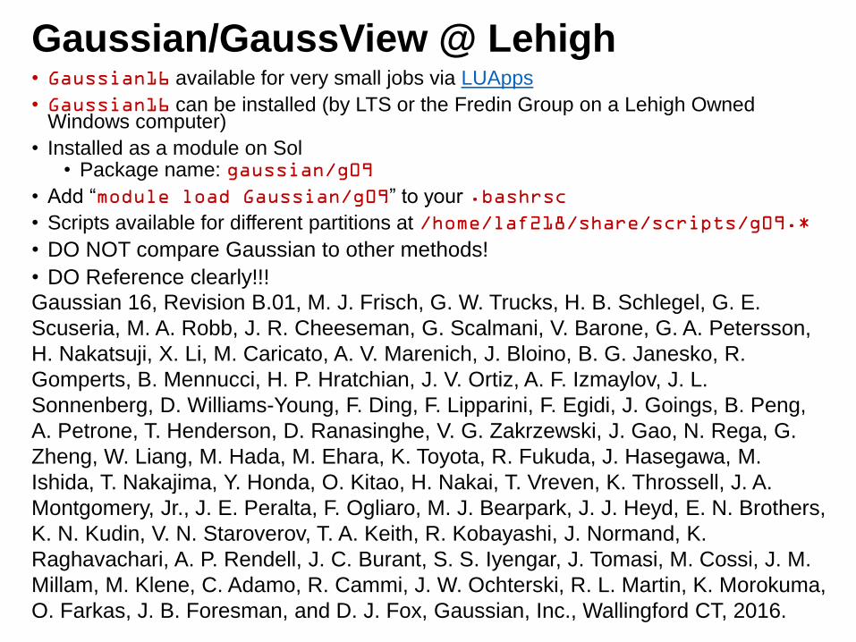
Gaussian/GaussView @ Lehigh• Gaussian16 available for very small jobs via LUApps

• Gaussian16 can be installed (by LTS or the Fredin Group on a Lehigh Owned Windows computer)

• Installed as a module on Sol• Package name: gaussian/g09

• Add “module load Gaussian/g09” to your .bashrsc

• Scripts available for different partitions at /home/laf218/share/scripts/g09.*

• DO NOT compare Gaussian to other methods!

• DO Reference clearly!!!

Gaussian 16, Revision B.01, M. J. Frisch, G. W. Trucks, H. B. Schlegel, G. E.

Scuseria, M. A. Robb, J. R. Cheeseman, G. Scalmani, V. Barone, G. A. Petersson,

H. Nakatsuji, X. Li, M. Caricato, A. V. Marenich, J. Bloino, B. G. Janesko, R.

Gomperts, B. Mennucci, H. P. Hratchian, J. V. Ortiz, A. F. Izmaylov, J. L.

Sonnenberg, D. Williams-Young, F. Ding, F. Lipparini, F. Egidi, J. Goings, B. Peng,

A. Petrone, T. Henderson, D. Ranasinghe, V. G. Zakrzewski, J. Gao, N. Rega, G.

Zheng, W. Liang, M. Hada, M. Ehara, K. Toyota, R. Fukuda, J. Hasegawa, M.

Ishida, T. Nakajima, Y. Honda, O. Kitao, H. Nakai, T. Vreven, K. Throssell, J. A.

Montgomery, Jr., J. E. Peralta, F. Ogliaro, M. J. Bearpark, J. J. Heyd, E. N. Brothers,

K. N. Kudin, V. N. Staroverov, T. A. Keith, R. Kobayashi, J. Normand, K.

Raghavachari, A. P. Rendell, J. C. Burant, S. S. Iyengar, J. Tomasi, M. Cossi, J. M.

Millam, M. Klene, C. Adamo, R. Cammi, J. W. Ochterski, R. L. Martin, K. Morokuma,

O. Farkas, J. B. Foresman, and D. J. Fox, Gaussian, Inc., Wallingford CT, 2016.

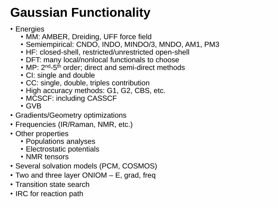
Gaussian Functionality• Energies

• MM: AMBER, Dreiding, UFF force field• Semiempirical: CNDO, INDO, MINDO/3, MNDO, AM1, PM3• HF: closed-shell, restricted/unrestricted open-shell• DFT: many local/nonlocal functionals to choose• MP: 2nd-5th order; direct and semi-direct methods• CI: single and double• CC: single, double, triples contribution• High accuracy methods: G1, G2, CBS, etc.• MCSCF: including CASSCF• GVB

• Gradients/Geometry optimizations

• Frequencies (IR/Raman, NMR, etc.)

• Other properties• Populations analyses• Electrostatic potentials• NMR tensors

• Several solvation models (PCM, COSMOS)

• Two and three layer ONIOM – E, grad, freq

• Transition state search

• IRC for reaction path

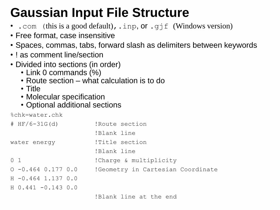
Gaussian Input File Structure• .com (this is a good default),.inp, or .gjf (Windows version)

• Free format, case insensitive

• Spaces, commas, tabs, forward slash as delimiters between keywords

• ! as comment line/section

• Divided into sections (in order)• Link 0 commands (%)• Route section – what calculation is to do• Title• Molecular specification• Optional additional sections

%chk=water.chk

# HF/6-31G(d) !Route section

!Blank line

water energy !Title section

!Blank line

0 1 !Charge & multiplicity

O -0.464 0.177 0.0 !Geometry in Cartesian Coordinate

H -0.464 1.137 0.0

H 0.441 -0.143 0.0

!Blank line at the end

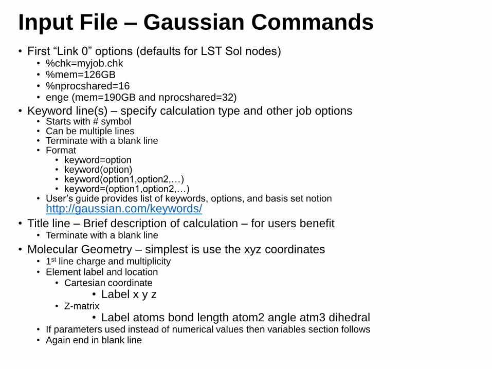
Input File – Gaussian Commands• First “Link 0” options (defaults for LST Sol nodes)

• %chk=myjob.chk• %mem=126GB• %nprocshared=16• enge (mem=190GB and nprocshared=32)

• Keyword line(s) – specify calculation type and other job options• Starts with # symbol• Can be multiple lines• Terminate with a blank line• Format

• keyword=option• keyword(option)• keyword(option1,option2,…)• keyword=(option1,option2,…)

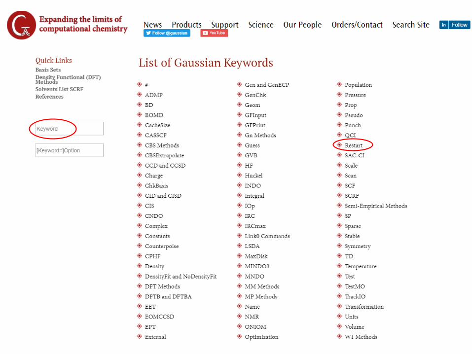
• User’s guide provides list of keywords, options, and basis set notionhttp://gaussian.com/keywords/

• Title line – Brief description of calculation – for users benefit• Terminate with a blank line

• Molecular Geometry – simplest is use the xyz coordinates• 1st line charge and multiplicity• Element label and location

• Cartesian coordinate

• Label x y z• Z-matrix

• Label atoms bond length atom2 angle atm3 dihedral• If parameters used instead of numerical values then variables section follows• Again end in blank line

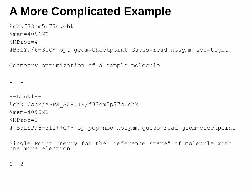
A More Complicated Example%chkf33em5p77c.chk

%mem=4096MB

%NProc=4

#B3LYP/6-31G* opt geom=Checkpoint Guess=read nosymm scf=tight

Geometry optimization of a sample molecule

1 1

--Link1--

%chk=/scr/APPS_SCRDIR/f33em5p77c.chk

%mem=4096MB

%NProc=2

# B3LYP/6-311++G** sp pop=nbo nosymm guess=read geom=checkpoint

Single Point Energy for the "reference state" of molecule with one more electron.

0 2

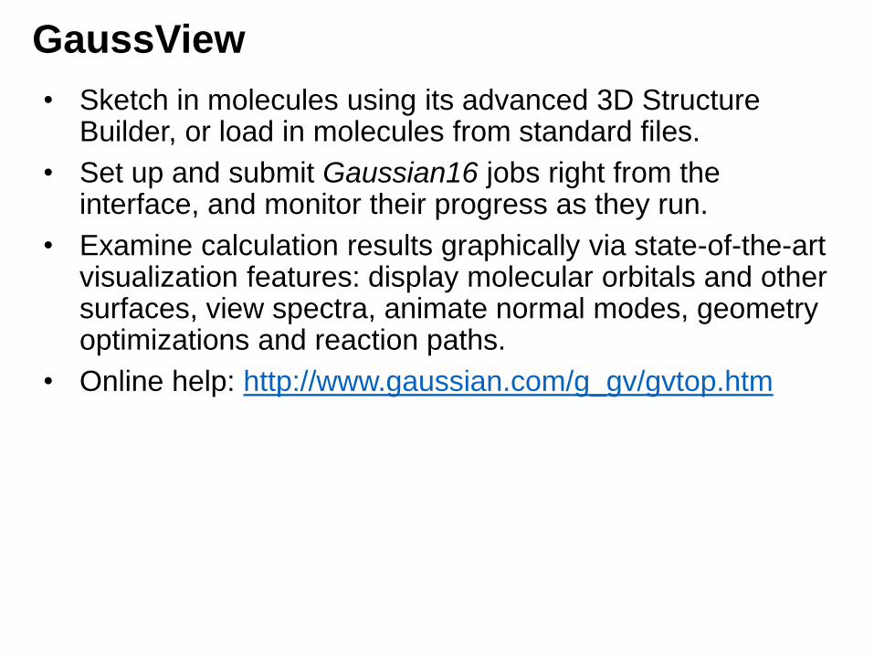
GaussView

• Sketch in molecules using its advanced 3D Structure Builder, or load in molecules from standard files.

• Set up and submit Gaussian16 jobs right from the interface, and monitor their progress as they run.

• Examine calculation results graphically via state-of-the-art visualization features: display molecular orbitals and other surfaces, view spectra, animate normal modes, geometry optimizations and reaction paths.

• Online help: http://www.gaussian.com/g_gv/gvtop.htm

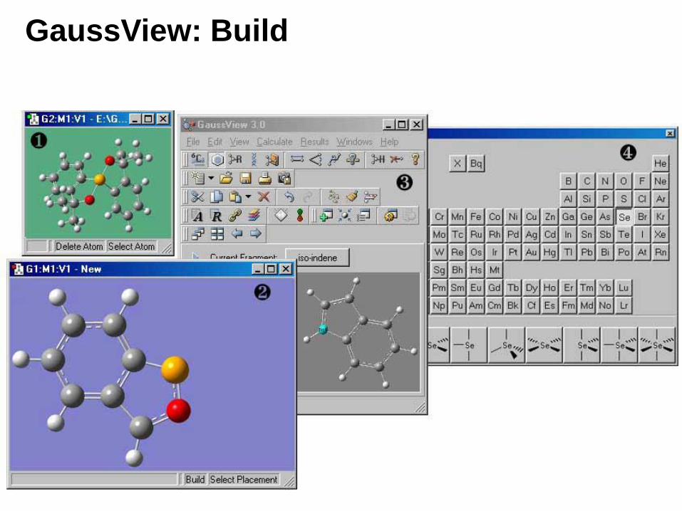
GaussView: Build

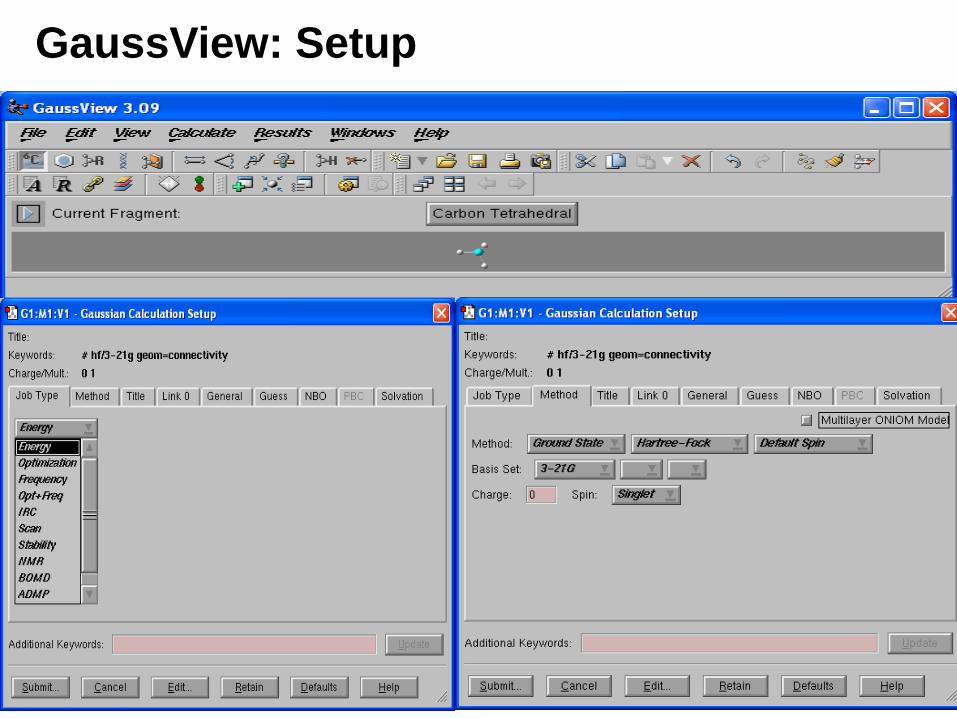
GuassView: Setup

• Molecule specification input is set up automatically.

• Specify additional redundant internal coordinates by clicking on the appropriate atoms and optionally setting the value.

• Specify the input for any Gaussian 03 calculation type. • Select the job from a pop-up menu. Related options automatically

appear in the dialog.• Select any method and basis set from pop-up menus.• Set up calculations for systems in solution. Select the desired solvent

from a pop-up menu.• Set up calculations for solids using the periodic boundary conditions

method. GaussView specifies the translation vectors automatically.• Set up molecule specifications for QST2 and QST3 transition state

searches using the Builder’s molecule group feature to transform one structure into the reactants, products and/or transition state guess.

• Select orbitals for CASSCF calculations using a graphical MO editor, rearranging the order and occupations with the mouse.

• Start and monitor local Gaussian jobs.

• Start remote jobs via a custom script.

GaussView: Setup

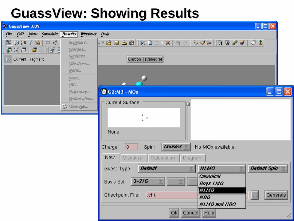
GuassView: Showing Results

• Show calculation results summary.

• Examine atomic changes: display numerical values or color atoms by charge (optionally selecting custom colors).

• Create surfaces for molecular orbitals, electron density, electrostatic potential, spin density, or NMR shielding density from Gaussian job results.

• Display as solid, translucent or wire mesh.

• Color surfaces by a separate property.

• Load and display any cube created by Gaussian 03.

• Animate normal modes associated with vibrational frequencies (or indicate the motion with vectors).

• Display spectra: IR, Raman, NMR, VCD.

• Display absolute NMR results or results with respect to an available reference compound.

• Animate geometry optimizations, IRC reaction path following, potential energy surface scans, and BOMD and ADMP trajectories.

• Produce web graphics and publication quality graphics files and printouts.

• Save/print images at arbitrary size and resolution.

• Create TIFF, JPEG, PNG, BMP and vector graphics EPS files.

• Customize element, surface, charge and background colors, or select high quality gray scale output.

GuassView: Showing Results

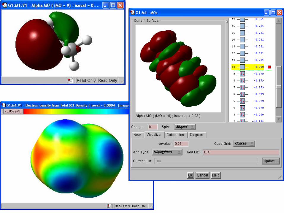
Surfaces

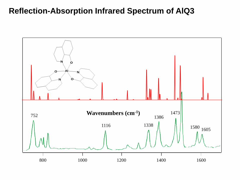
Reflection-Absorption Infrared Spectrum of AlQ3

ON

AlO

ON

N

752

1116 1338

13861473

15801605

160014001200800 1000

Wavenumbers (cm-1)

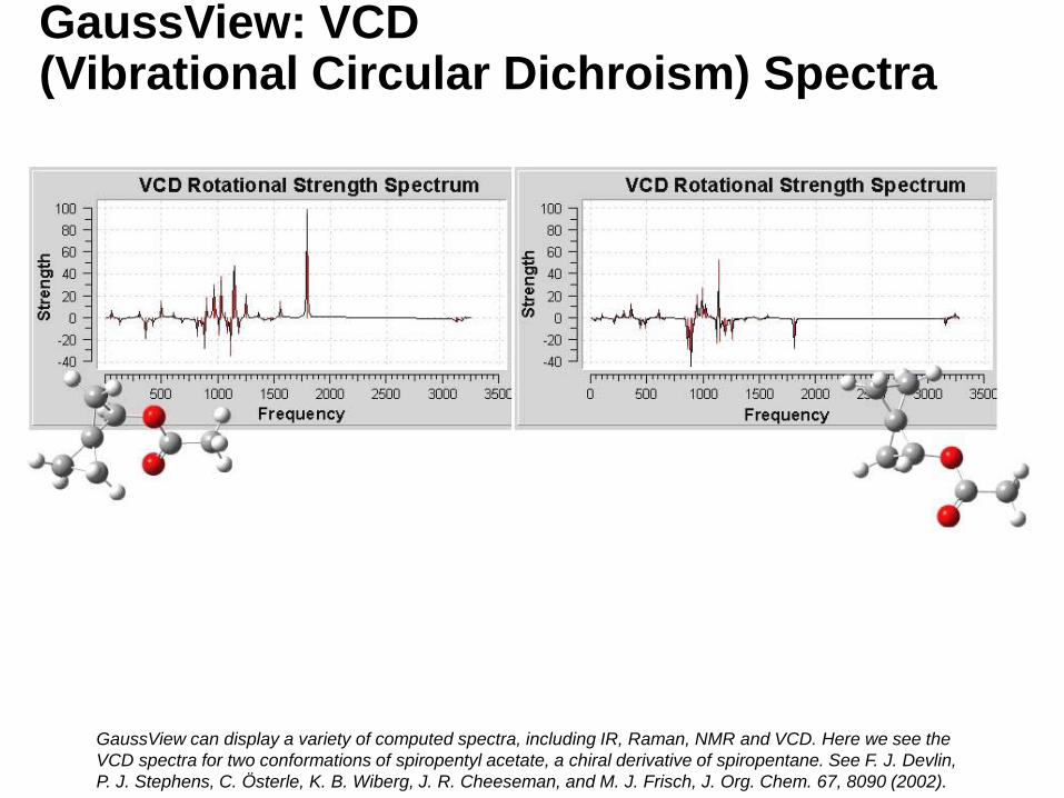
GaussView: VCD (Vibrational Circular Dichroism) Spectra

GaussView can display a variety of computed spectra, including IR, Raman, NMR and VCD. Here we see the

VCD spectra for two conformations of spiropentyl acetate, a chiral derivative of spiropentane. See F. J. Devlin,

P. J. Stephens, C. Österle, K. B. Wiberg, J. R. Cheeseman, and M. J. Frisch, J. Org. Chem. 67, 8090 (2002).

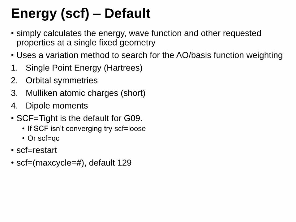
Energy (scf) – Default

• simply calculates the energy, wave function and other requested properties at a single fixed geometry

• Uses a variation method to search for the AO/basis function weighting

1. Single Point Energy (Hartrees)

2. Orbital symmetries

3. Mulliken atomic charges (short)

4. Dipole moments

• SCF=Tight is the default for G09. • If SCF isn’t converging try scf=loose

• Or scf=qc

• scf=restart

• scf=(maxcycle=#), default 129

Functionals

• A functional is just a function that depends on a function

• Local density approximation (LDA): Functional depends only on the (local) density at a given point.

• Example: SVWN

• Gradient-corrected approximation (GGA): Functional depends on local density and its gradient.

• Examples: PW91 and LYP correlation functionals, B88 exchange functional

• Meta-GGA: Functional depends on density, its gradient, and its second derivative.

• Example: M06-L

• Hybrid DFT: Mixes in Hartree-Fock exchange. • Most popular example: B3LYP (hybrid GGA). M05-2X and M06-2X are hybrid

meta-GGA’s.

Beyond HF

• Hartree Potential: each individual electron moves independently of each other, only feeling the average electrostatic field due to all the other electrons plus the field due to the atoms.

• neglects exchange and correlation effects.

• Kohn-Sham: Compute the kinetic energy of a density by assuming that the density corresponds to a wavefunction consisting of a single Slater determinant (“non-interacting limit”): we know how to compute the kinetic energy of a Slater determinant (orbitals) --- looks same as HartreeFockTheory

• Exchange-Correlation Functional: We can compute every piece of a Kohn-Sham DFT energy exactly except for the “exchange correlation” piece, Exc[ρ]. (still KS)

• Unfortunately the exact exchange-correlation energy functional is not known and is probably so complicated that even if it were known it would not be computationally useful

• Hence, use various approximate exchange correlation functionals (S-VWN, B3LYP, etc.)

• KS cost is similar to HF (similar equations) but quality can be better because correlation is built in through the correlation functional

• Cost can actually be cheaper than HF if we replace the expensive, long-range exchange integrals (K terms) from HF with a shorter range exchange potential (which however might not be as accurate…)

Basis Set

• Minimal basis set (e.g., STO-3G)

• Double zeta basis set (DZ)

• Split valence basis Set (e.g., 6-31G)

• K-LMG• K = number of sp-type inner shell GTOs

• L = number of inner valence s- and p-type GTOs

• M = number of outer valence s- and p-type GTOs

• G = indicates that GTOs are used

• Polarization and diffuse functions (6-31+G*)

• Correlation-consistent basis functions (e.g., aug-cc-pvTZ)

• Pseudopotentials, effective core potentials

https://gaussian.com/basissets/

Geometry (opt)

• calculates the wave function and the energy at a starting geometry

• calculates the force on each atom by evaluating the gradient (first derivative) of the energy with respect to atomic positions

• Minimal energy when the force is below some threshold

1. Atomic coordinates of optimized molecule

2. Optimized Parameters: atomic distances and angles

3. HOMO/LUMO eigenvalues (Hartrees)

4. Mulliken atomic charges (short)

5. Dipole moments

Tricks:

• If the first scf is taking a long time (over 500 steps) try a new guess

• Use maxstep=# to change the size of steps taken in opt

• Always check the freq for imaginary frequencies (negative)

Stable?

• The stability calculation determines whether the wavefunctioncomputed for the molecular system is stable or not:

• in other words, whether there is a lower energy wavefunction corresponding to a different solution of the SCF equations.

• If the wavefunction is unstable, then whatever calculation you are performing is not being done on the expected/desired state of the molecule.

• SCF = self consistent field

• DFT = density functional theory

• Stable=Opt the wavefunction is allowed to be unrestricted if necessary

• Stable geometry message• The wavefunction is stable under the perturbations considered.

• Unstable geometry messages• The wavefunction has an RHF → UHF instability.

• The wavefunction has internal instability.

Vibrational Spectroscopy & Thermochemistry (freq)

• calculate the vibrations of the molecule in question, along with other parameters that you can choose to include or

erase from the output

• molecular frequencies depend on the second derivative of the energy with respect to the nuclear positions

• NOTE: You must use the same combination of theoretical model and basis set for both the Opt

and Freq calculations

1. Atomic coordinates of optimized molecule

2. Optimized parameters: atomic distances and angles

3. HOMO/LUMO eigenvalues (hartree)

4. Mulliken atomic charges (short)

5. Dipole moments

6. Single Point energy

7. Harmonic frequnecies (wavenumbers)

8. Reduced masses (amu)

9. Force constants

10. IR intensities

11. Raman intensities (not default)

12. Thermochemistry(a) Temperature

(b) Pressure

(c) Isotopes used

(d) Molecular mass

(e) Thermal energy: E (Thermal)

(f) Constant volume molar heat capacity (CV)

(g) Entropy (S)

(h) Free Energy (sum of electronic and thermal Free Energies)

(i) Enthalpy (sum of electronic and thermal Enthalpies)

http://gaussian.com/vib/

freq results

1. SCALING depends on the theoretical method and basis set used. Note that the scaling

factors for frequencies and for zero point energies are different! You can input the scale

factor to be used for thermochemistry analysis using the Scale keyword (ex: "Scale=0.95")

• https://cccbdb.nist.gov/vibscalejust.asp

2. STABILITY imaginary (negative) frequencies. Imaginary frequencies indicate instability of

molecular geometry.

• each molecule should have either 3N-6 or 3N-5 vibrational modes

• The others are the translational and rotational modes and their intensities should close to zero (+/- 10)

• Big intensities for these frequencies is another way to verify the stability of you molecule

3. IMAGINARY FREQUENCIES saddle points on the potential energy surface

• a transition state should have one (1st order saddle point)

4. ANHARMONIC FREQUENCIES By default, G09 computes frequencies based on harmonic

oscillator approximation (second order derivative with respect to the nuclei movement).

• anharmonic corrections, i.e. computing higher-order derivatives. anharmonic" keyword

5. RAMAN "Raman" keyword

6. THERMOCHEMSITRY By default, several thermodynamic values are computed

during a vibrational analysis. You can change the thermochemistry

parameters (temperature, pressure, ect) by writing Freq=ReadIsotopes in the

Route section.

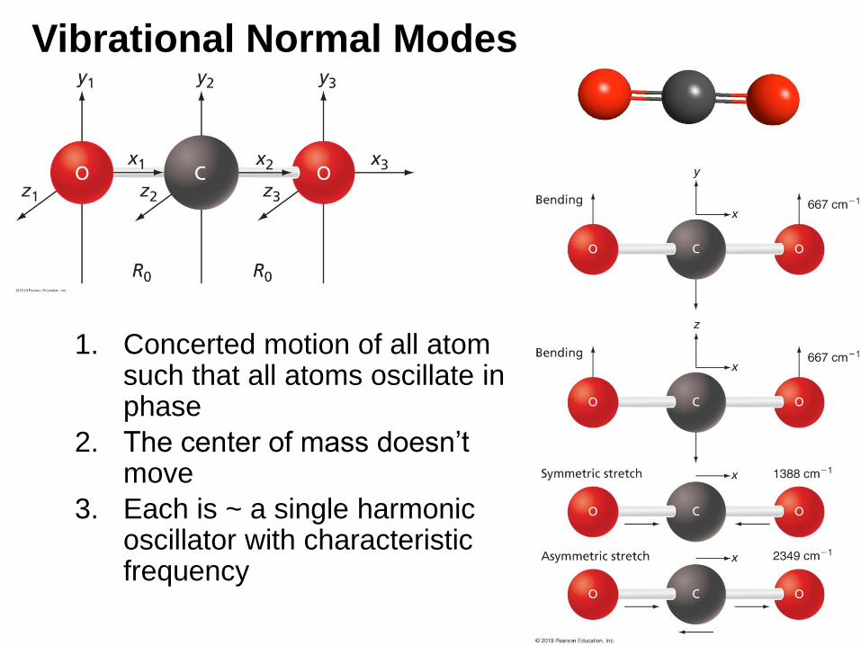
Vibrational Normal Modes

1. Concerted motion of all atom such that all atoms oscillate in phase

2. The center of mass doesn’t move

3. Each is ~ a single harmonic oscillator with characteristic frequency

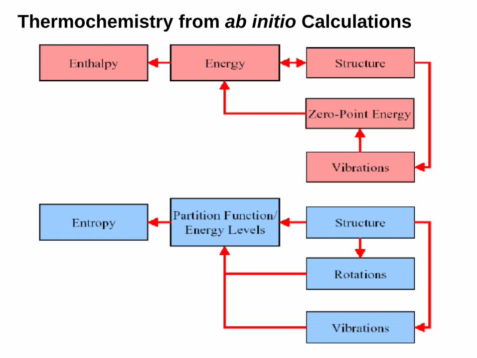
Thermochemistry from ab initio Calculations

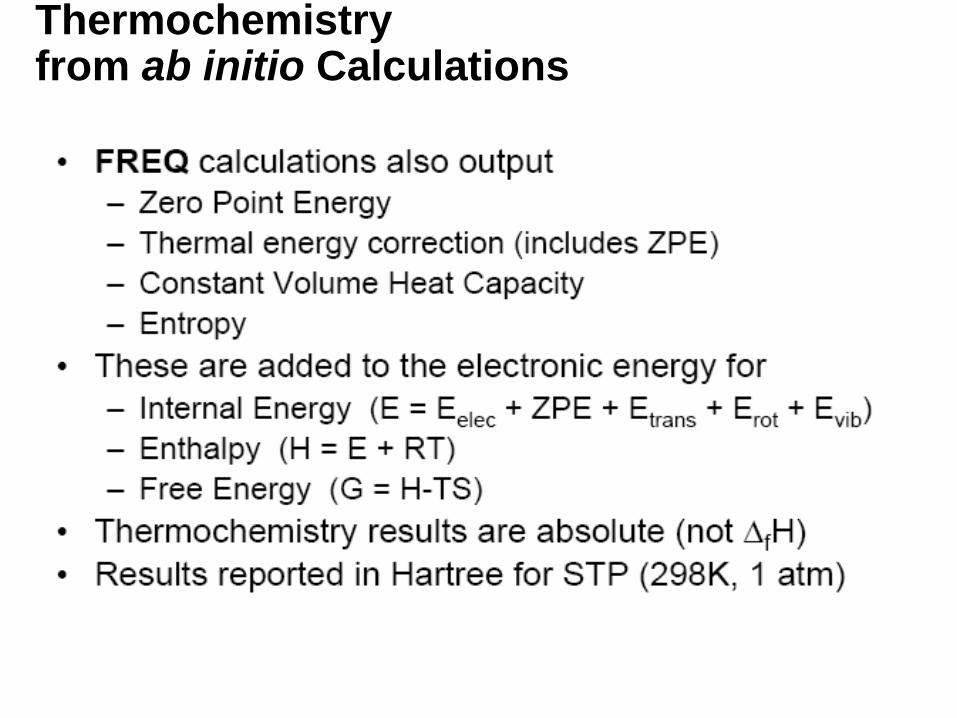
Thermochemistryfrom ab initio Calculations

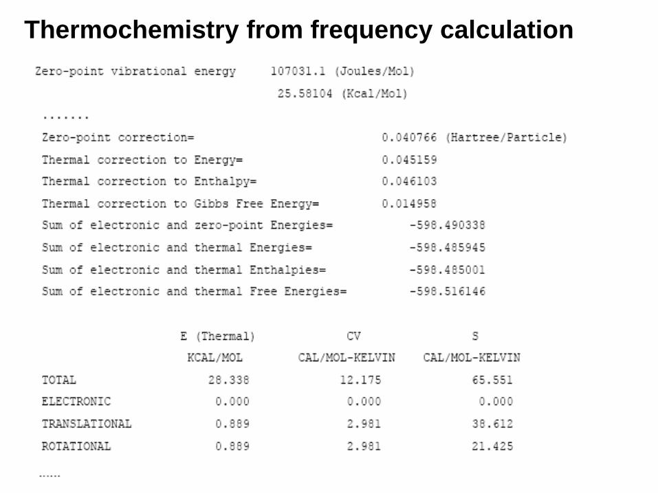
Thermochemistry from frequency calculation

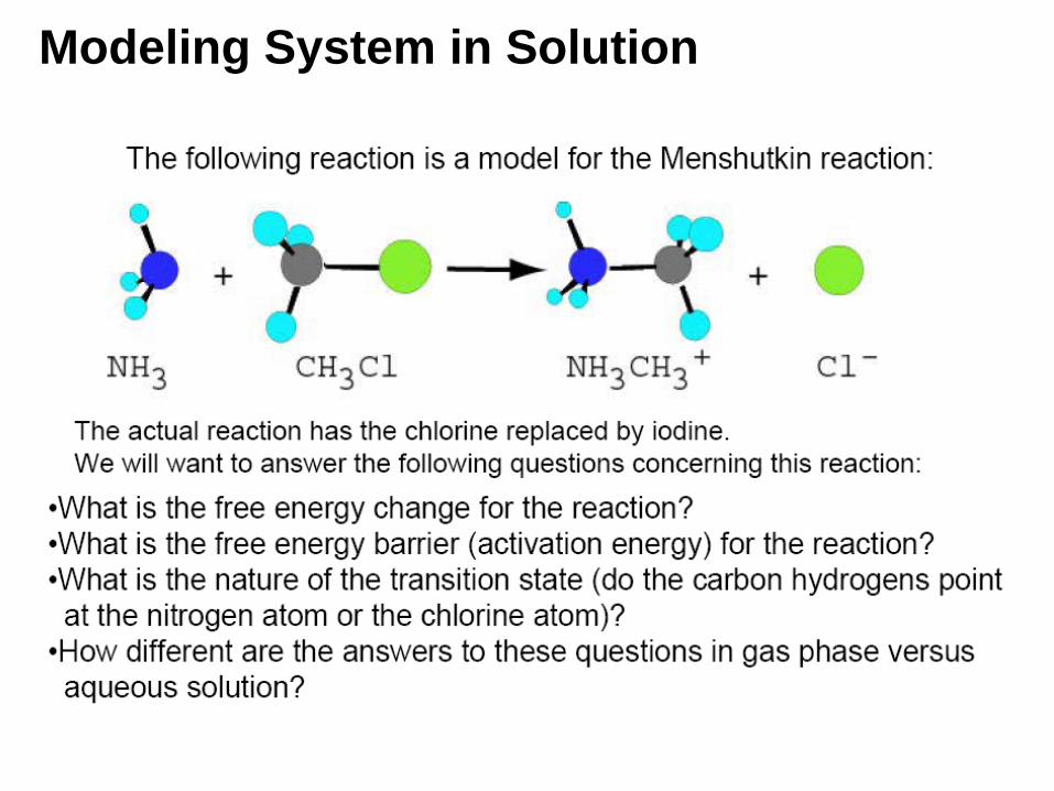
Modeling System in Solution

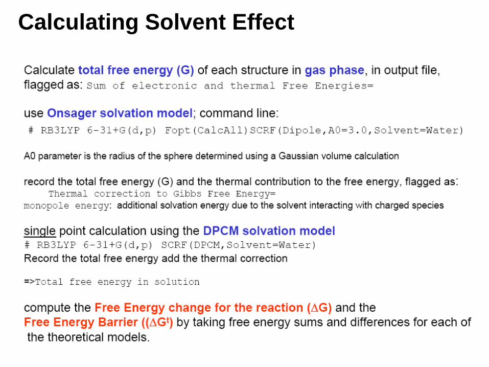
Calculating Solvent Effect

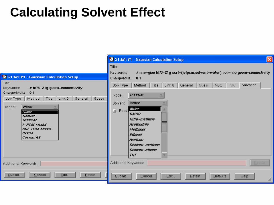
Calculating Solvent Effect

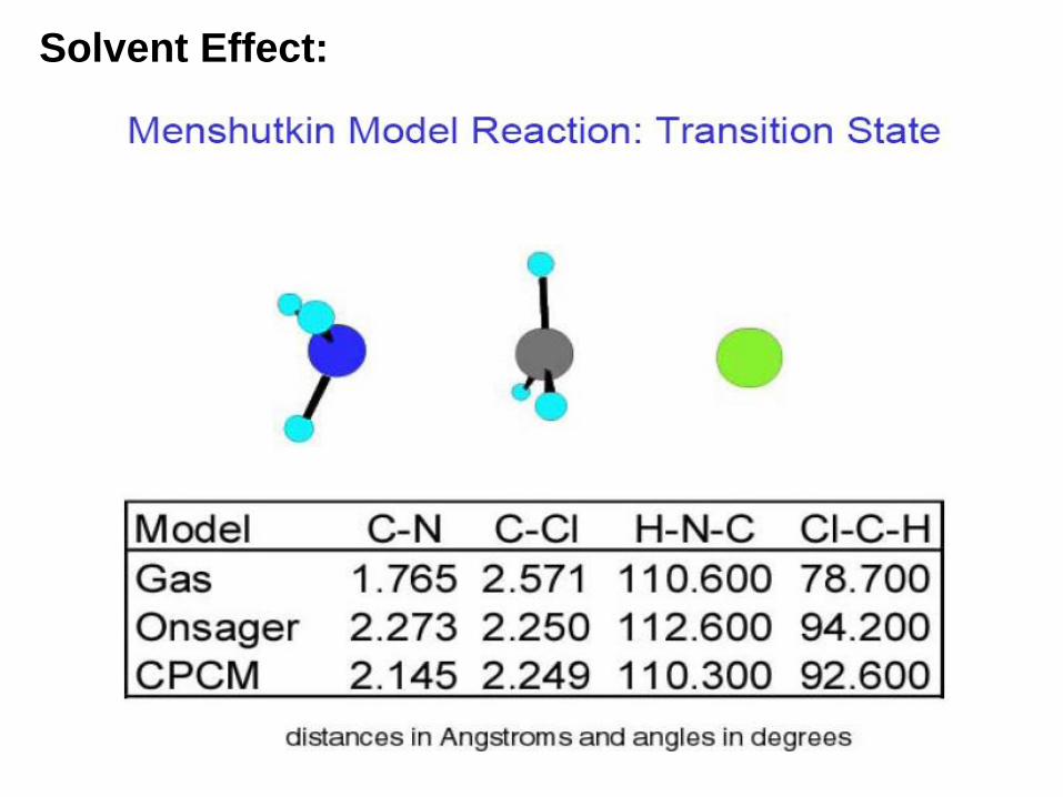
Solvent Effect:

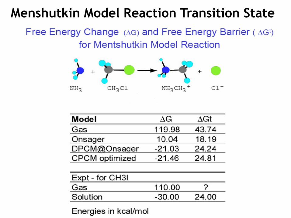
Menshutkin Model Reaction Transition State

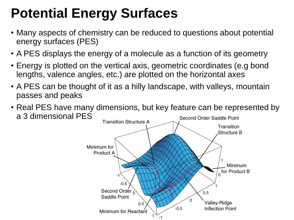
Potential Energy Surfaces

• Many aspects of chemistry can be reduced to questions about potential energy surfaces (PES)

• A PES displays the energy of a molecule as a function of its geometry

• Energy is plotted on the vertical axis, geometric coordinates (e.g bond lengths, valence angles, etc.) are plotted on the horizontal axes

• A PES can be thought of it as a hilly landscape, with valleys, mountain passes and peaks

• Real PES have many dimensions, but key feature can be represented by a 3 dimensional PES

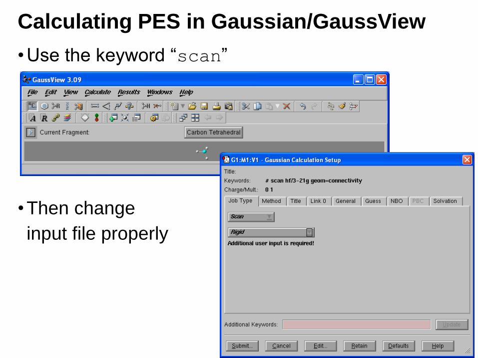
Calculating PES in Gaussian/GaussView

•Use the keyword “scan”

•Then change

input file properly

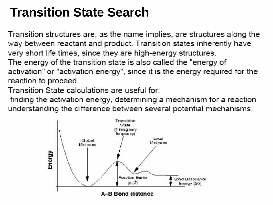
Transition State Search

Calculating Transition States

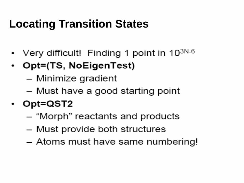
Locating Transition States

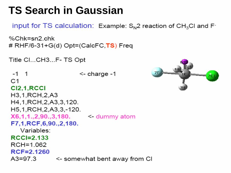
TS Search in Gaussian

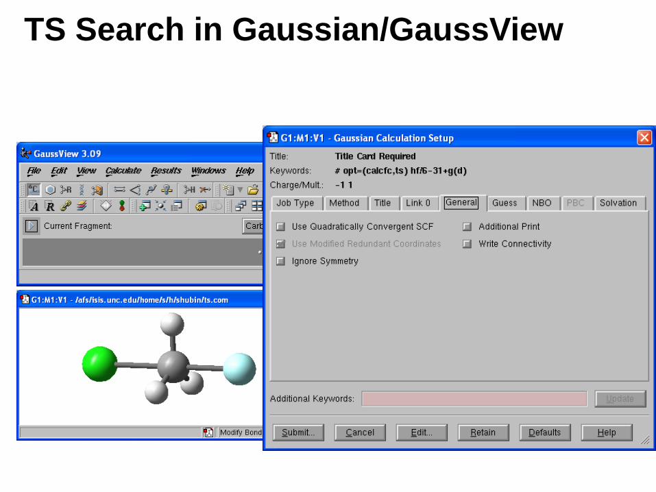
TS Search in Gaussian/GaussView

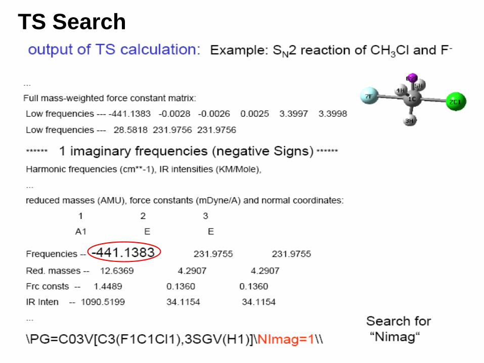
TS Search

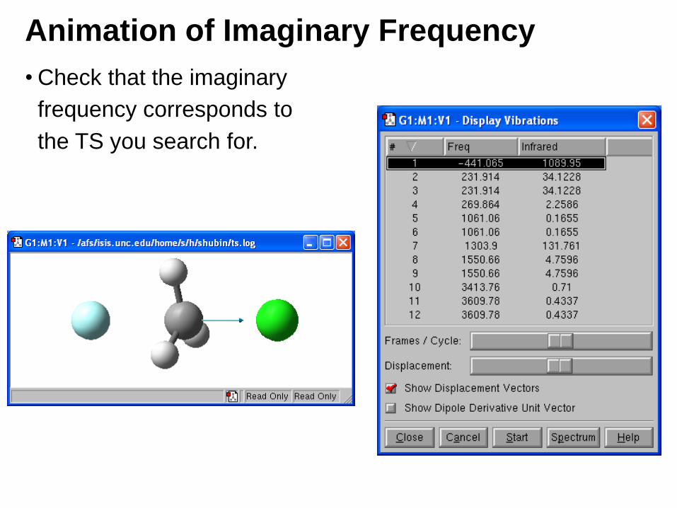
Animation of Imaginary Frequency

• Check that the imaginary

frequency corresponds to

the TS you search for.

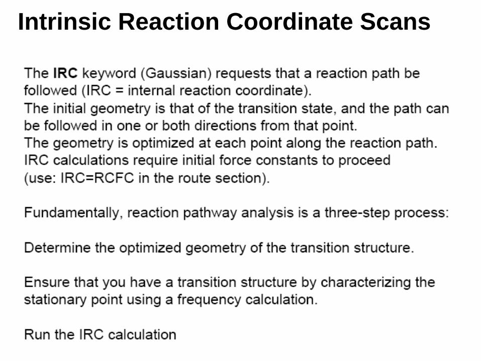
Intrinsic Reaction Coordinate Scans

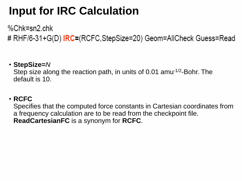
Input for IRC Calculation

• StepSize=N Step size along the reaction path, in units of 0.01 amu-1/2-Bohr. The default is 10.

• RCFC Specifies that the computed force constants in Cartesian coordinates from a frequency calculation are to be read from the checkpoint file. ReadCartesianFC is a synonym for RCFC.

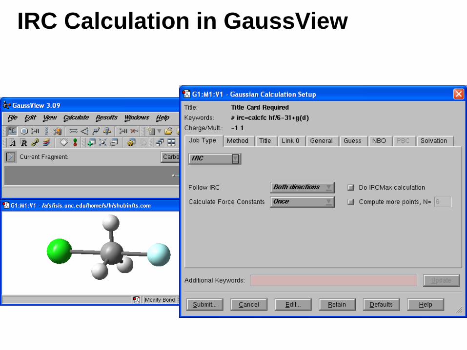
IRC Calculation in GaussView

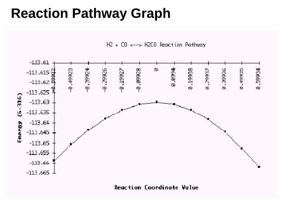
Reaction Pathway Graph

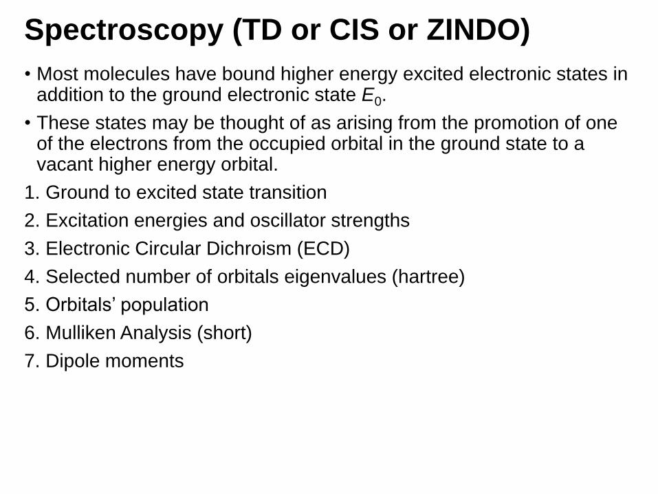
Spectroscopy (TD or CIS or ZINDO)

• Most molecules have bound higher energy excited electronic states in addition to the ground electronic state E0.

• These states may be thought of as arising from the promotion of one of the electrons from the occupied orbital in the ground state to a vacant higher energy orbital.

1. Ground to excited state transition

2. Excitation energies and oscillator strengths

3. Electronic Circular Dichroism (ECD)

4. Selected number of orbitals eigenvalues (hartree)

5. Orbitals’ population

6. Mulliken Analysis (short)

7. Dipole moments

Spectroscopy (TD or CIS or ZINDO)

• The classical Franck-Condon principle states that because the rearrangement of electrons is much faster than the motion of nuclei, the nuclear configuration does not change significantly during the energy absorption process.

• Thus, the absorption spectrum (UV/Vis) of molecules is characterized by the vertical excitation energies.

• TDDFT in general (singlets and triplets)• Time Dependent calculation based on a DFT computational method.

• obtains the wave functions of MOs that oscillate between ground state and the first excited states.

• td(nstates=#,type)

• default is 3 and singlets

• At least 40 states are normally needed to calculate a UV-Vis

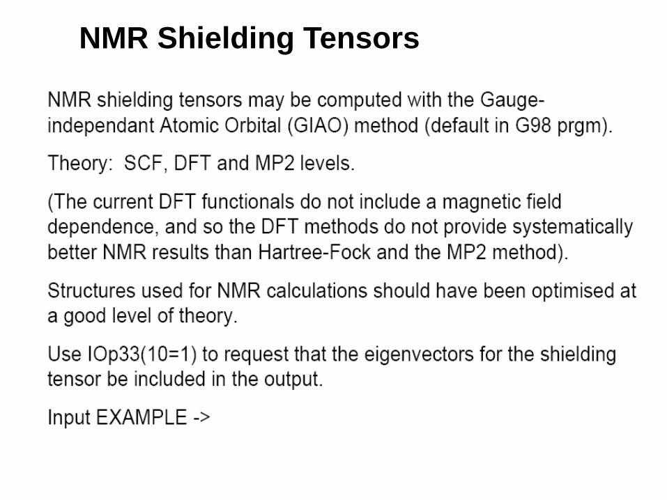
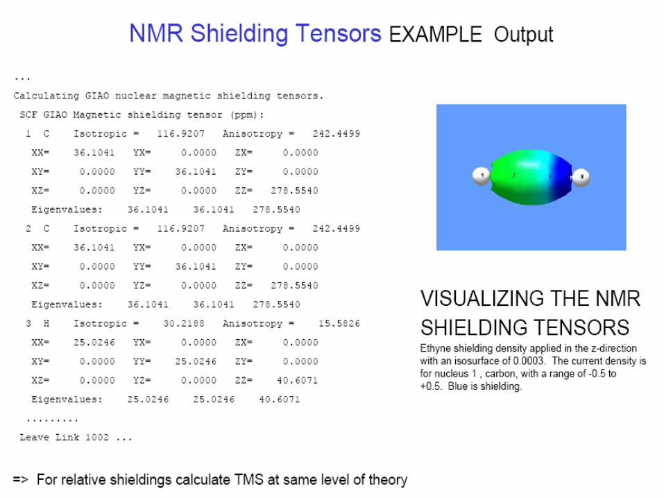
NMR Shielding Tensors

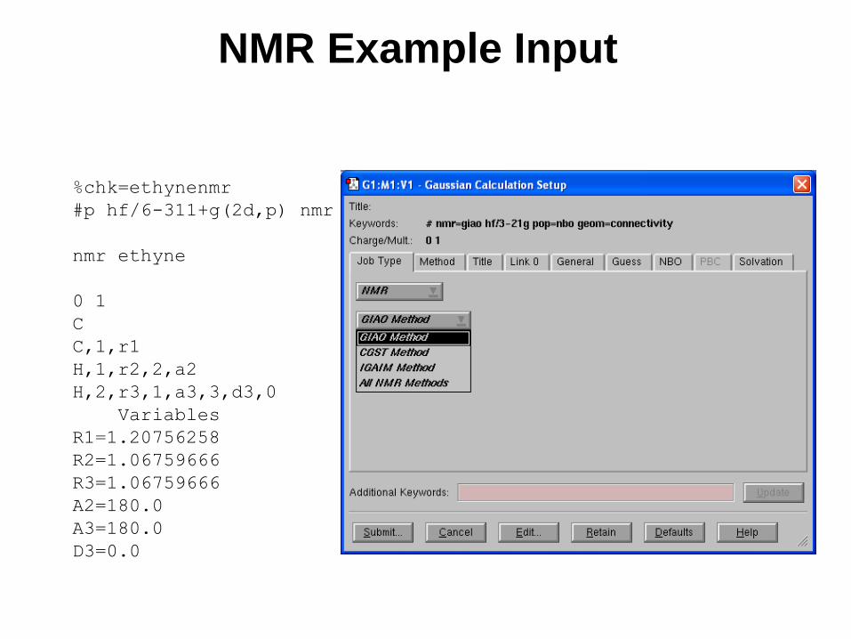
NMR Example Input

%chk=ethynenmr

#p hf/6-311+g(2d,p) nmr

nmr ethyne

0 1

C

C,1,r1

H,1,r2,2,a2

H,2,r3,1,a3,3,d3,0

Variables

R1=1.20756258

R2=1.06759666

R3=1.06759666

A2=180.0

A3=180.0

D3=0.0

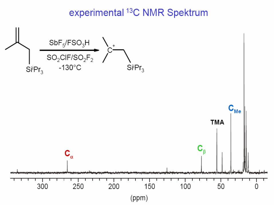
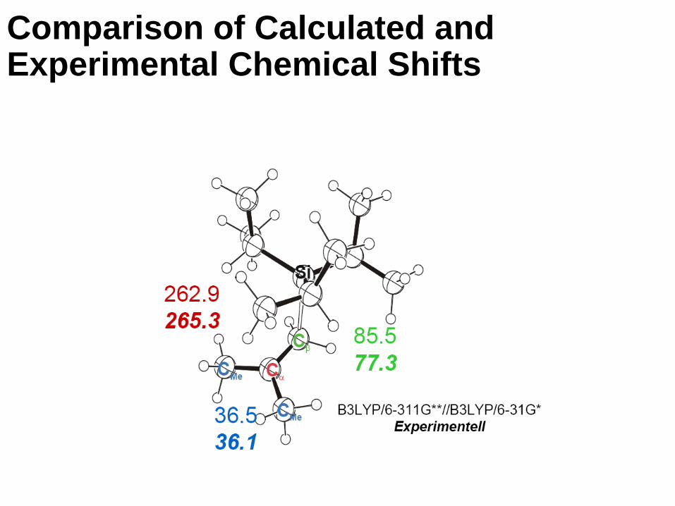
Comparison of Calculated and Experimental Chemical Shifts

Other Gaussian Utilities

• formchk – formats checkpoint file so it can be used by other programs

• cubgen – generate cube file to look at MOs, densities, gradients, NMR in GaussView

• freqchk – retrieves frequency/thermochemsitry data from chk file

• newzmat – converting molecular specs between formats (zmat, cart, chk, cache, fraccoord, MOPAC, pdb, and others)

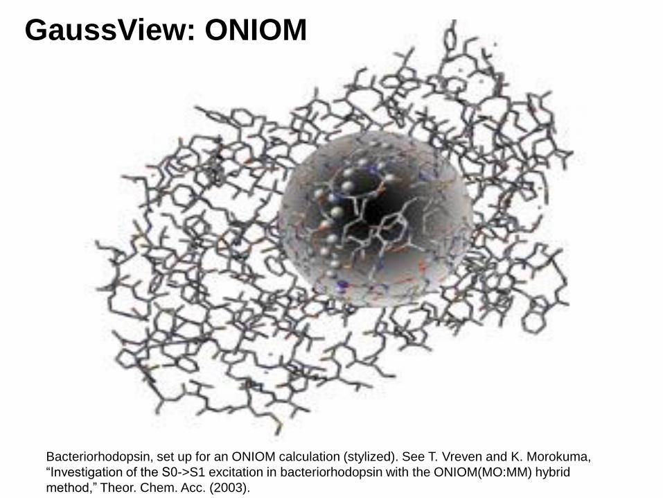
GaussView: ONIOM

Bacteriorhodopsin, set up for an ONIOM calculation (stylized). See T. Vreven and K. Morokuma,

“Investigation of the S0->S1 excitation in bacteriorhodopsin with the ONIOM(MO:MM) hybrid

method,” Theor. Chem. Acc. (2003).

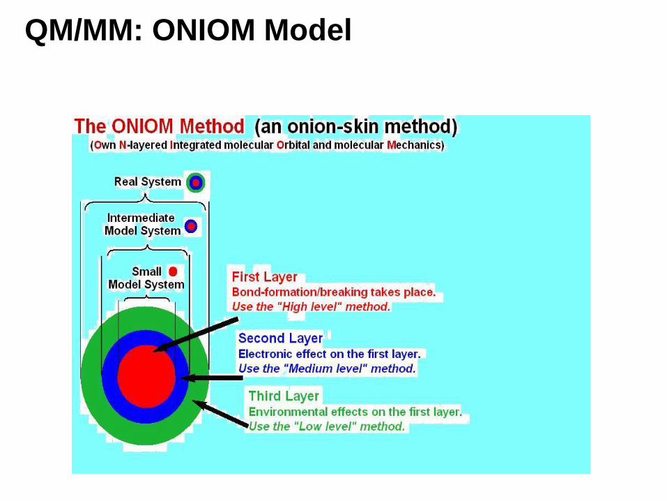
QM/MM: ONIOM Model

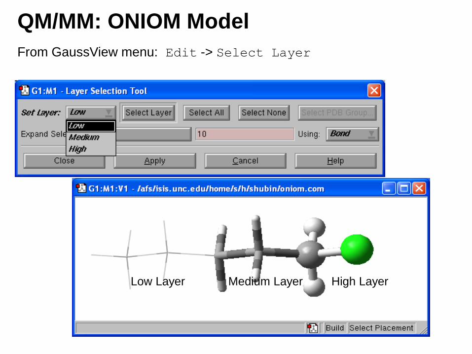
QM/MM: ONIOM Model

From GaussView menu: Edit -> Select Layer

Low Layer Medium Layer High Layer

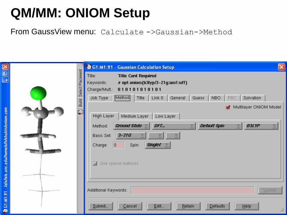
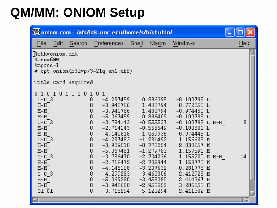
QM/MM: ONIOM Setup

From GaussView menu: Calculate ->Gaussian->Method

QM/MM: ONIOM Setup

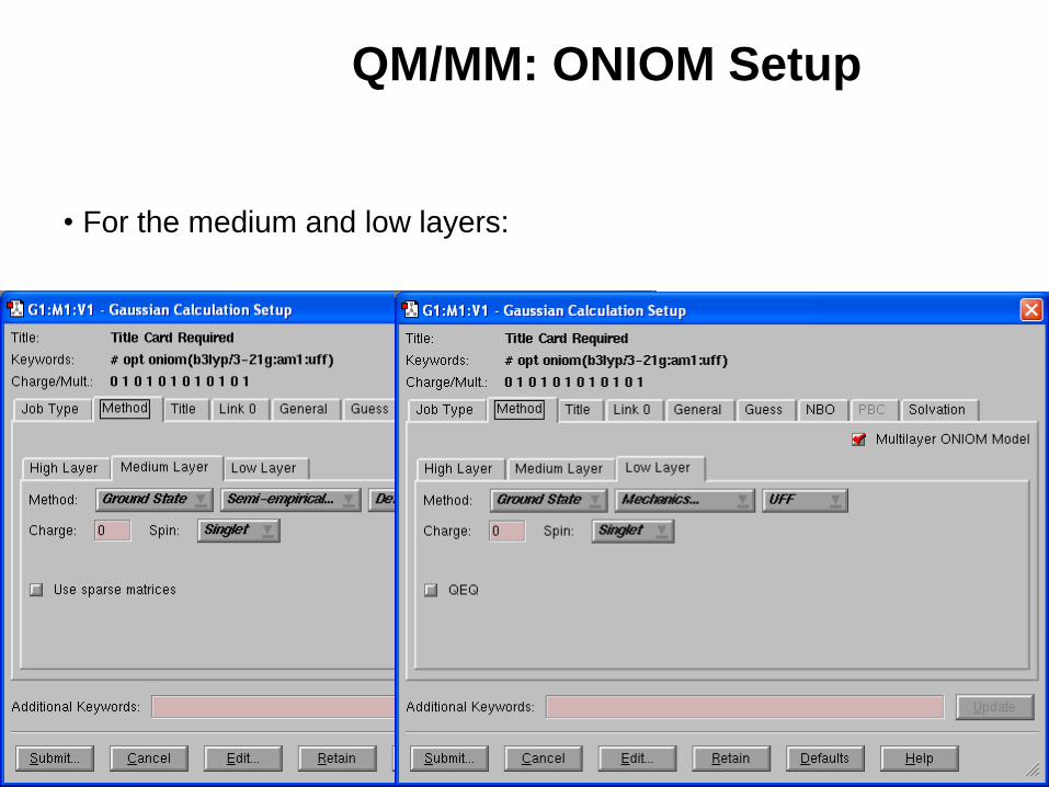
• For the medium and low layers:

QM/MM: ONIOM Setup

Population analysis

• a mathematical way of partitioning a wave function or electron density into charges on the nuclei, bond orders, and other related information.

• Atomic charges cannot be observed experimentally because they do not correspond to any unique physical property.

• In reality, atoms have a positive nucleus surrounded by negative electrons, not partial charges on each atom.

• However, condensing electron density and nuclear charges down to partial charges on the nucleus results in an understanding of the electron density distribution.

• These are not integer formal charges, but rather fractions of an electron corresponding to the percentage of time an electron is near each nucleus.

• Population are done once for SP energy calculation and at the first and last step of geometry optimization.

1. Atomic coordinates of optimized molecule

2. Optimized parameters: atomic distances and angles

3. Selected number of orbitals eigenvalues (hartree)

4. Orbitals’ population

5. Atomic (partial) charges (full analysis)

6. Dipole moment

7. Single Point energy

8. Electrostatic potential derived charges (with ESP keyword)

Pop=X keyword• PARTIAL CHARGES :

• Mulliken analysis is most common, • it is also one of the worst and is used only because it is one of the oldest and

simplest. • half the overlap population is assigned to each contributing orbital, giving the total

population of each AO. Summing over all the atomic orbitals on a specific atom gives us the gross atomic population.

• WARNING! Mulliken method is extremely basis set sensitive! Usually, the smaller the basis set, the better (opposite for energy calculations).

• X=NONE no orbital information displayed

• X=REG HOMO-5 up to LUMO+5 orbital information displayed

• X=FULL all orbitals information displayed

• X=NBO Mulliken analysis is replaced by Natural Bond-Order analysis• NBOs are an orthonormal set of localized "maximum occupancy“ orbitals

whose leading N/2 members (or N members in the open-shell case) give the most accurate possible Lewis-like description of the total N-electron density.

• NBO uses eigenfunctions of the first order reduced density matrix, localized and orthogonalized.

• X=MK, CHELP, OR CHELPG produce charges fit to electrostatic potential (ESP)

• ESP This method uses electrostatic potential to compute charges on nuclei. ESP is usually the best to describe charge interactions with other species, but require significant amount of CPU time.

What Is NBO?

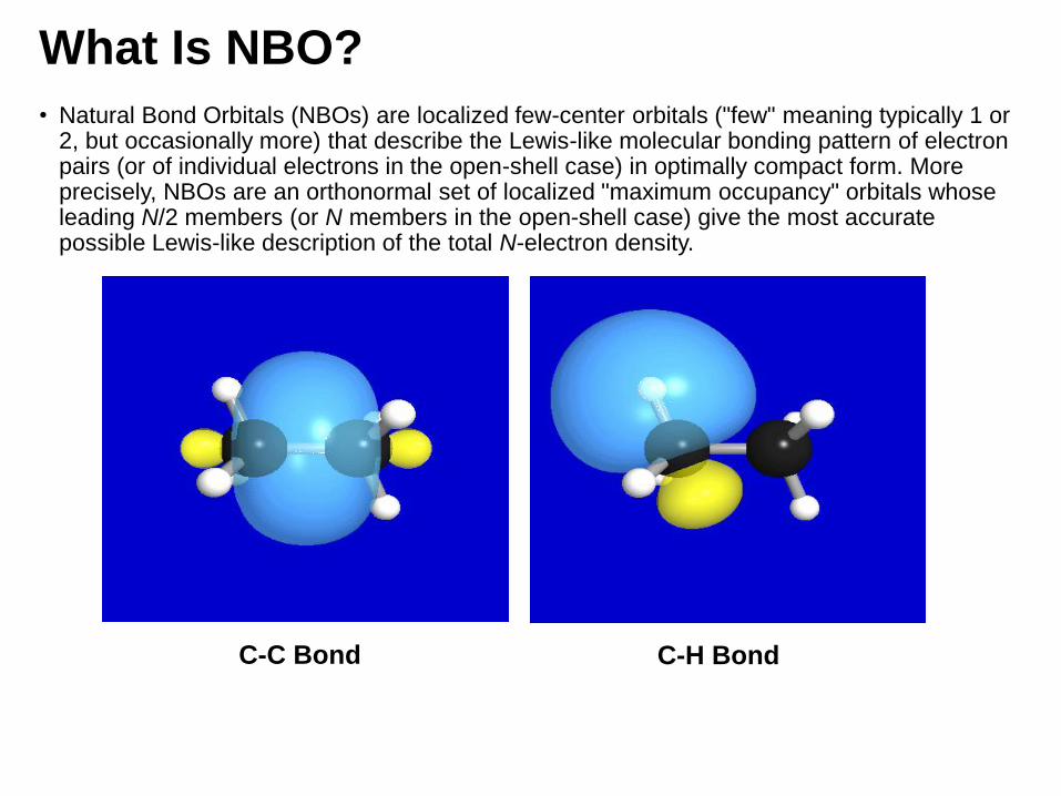
• Natural Bond Orbitals (NBOs) are localized few-center orbitals ("few" meaning typically 1 or 2, but occasionally more) that describe the Lewis-like molecular bonding pattern of electron pairs (or of individual electrons in the open-shell case) in optimally compact form. More precisely, NBOs are an orthonormal set of localized "maximum occupancy" orbitals whose leading N/2 members (or N members in the open-shell case) give the most accurate possible Lewis-like description of the total N-electron density.

C-C Bond C-H Bond

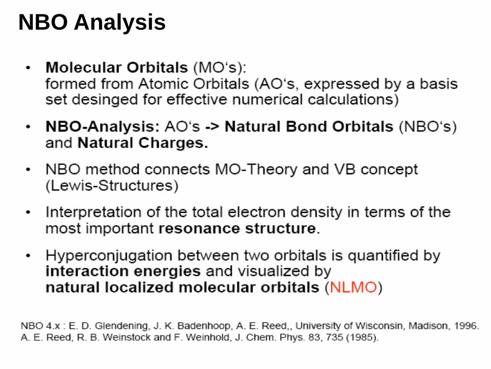
NBO Analysis

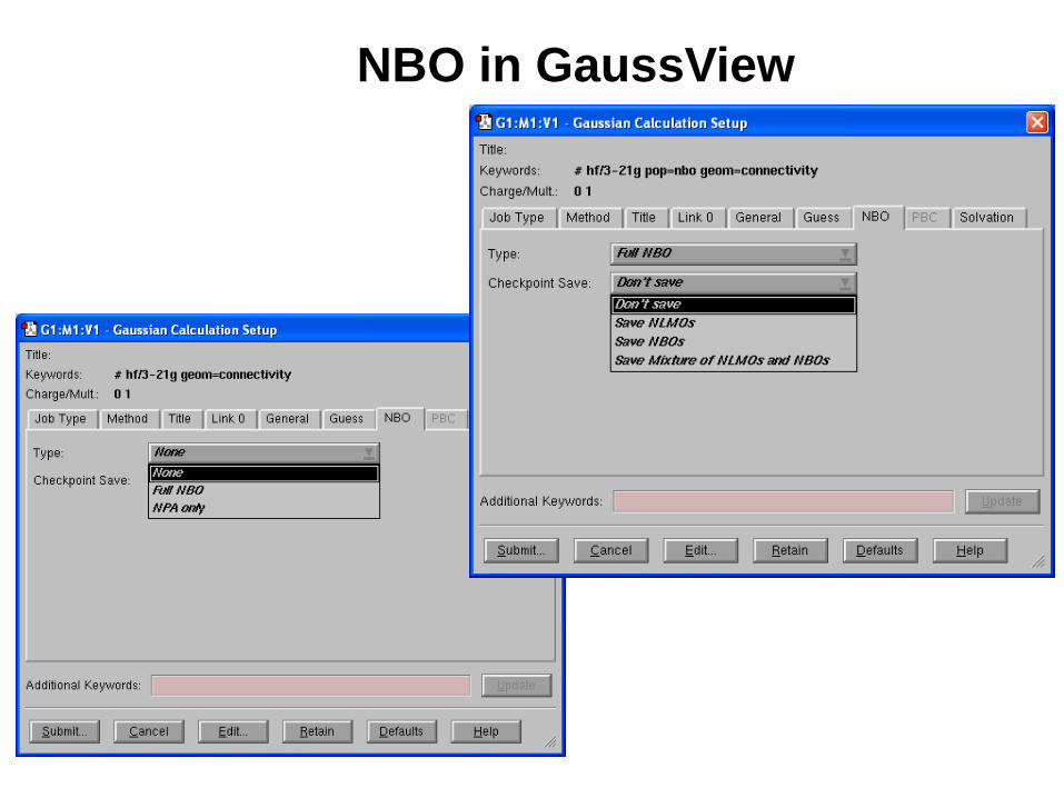
NBO in GaussView

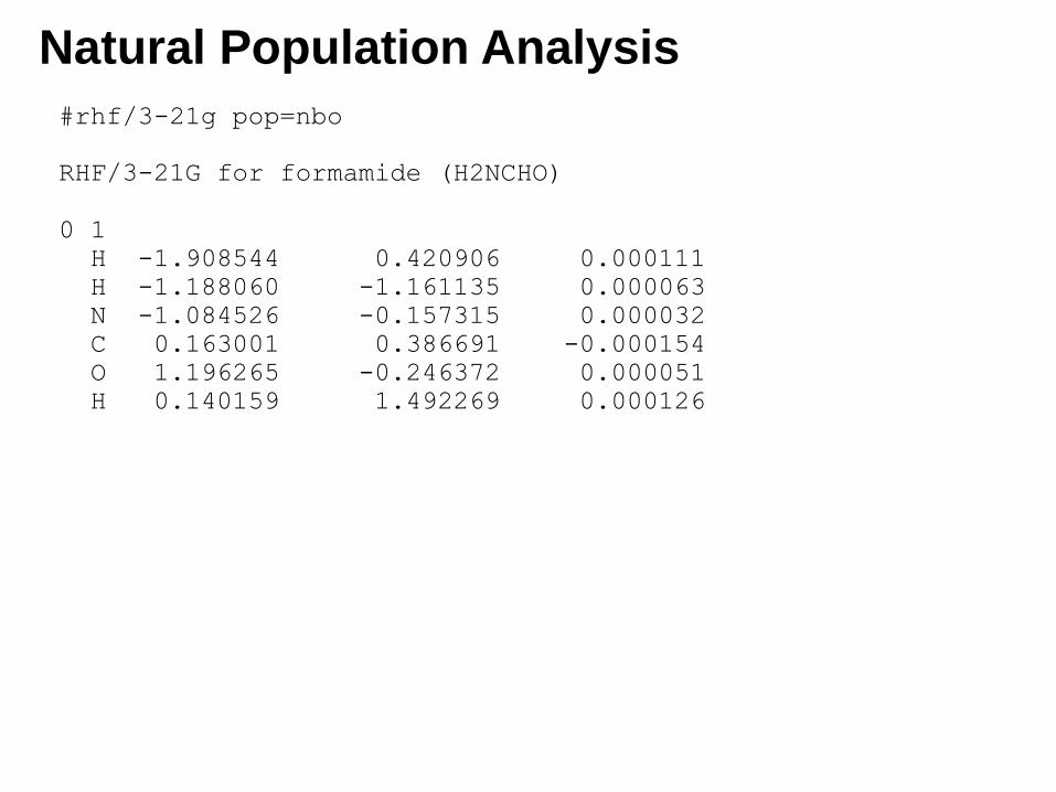
Natural Population Analysis

#rhf/3-21g pop=nbo

RHF/3-21G for formamide (H2NCHO)

0 1

H -1.908544 0.420906 0.000111

H -1.188060 -1.161135 0.000063

N -1.084526 -0.157315 0.000032

C 0.163001 0.386691 -0.000154

O 1.196265 -0.246372 0.000051

H 0.140159 1.492269 0.000126

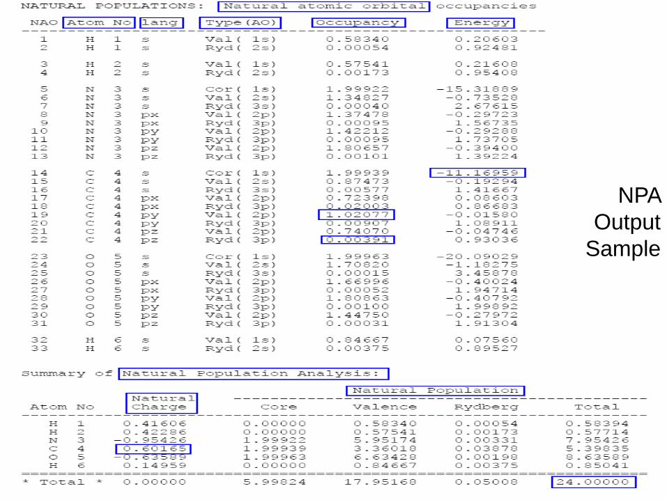
NPA

Output

Sample

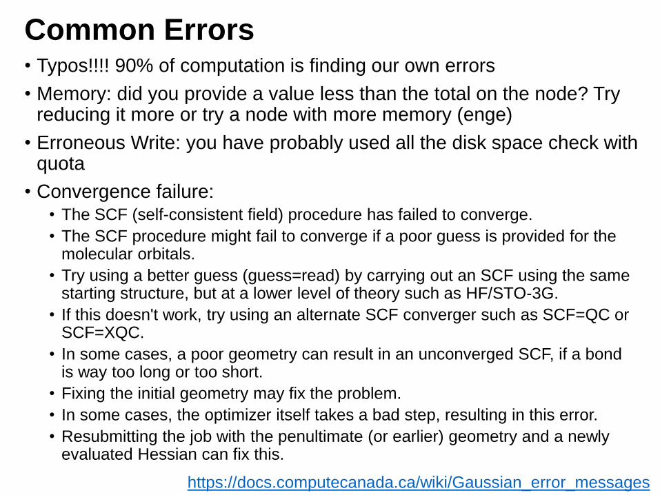
Common Errors• Typos!!!! 90% of computation is finding our own errors

• Memory: did you provide a value less than the total on the node? Try reducing it more or try a node with more memory (enge)

• Erroneous Write: you have probably used all the disk space check with quota

• Convergence failure:• The SCF (self-consistent field) procedure has failed to converge.

• The SCF procedure might fail to converge if a poor guess is provided for the molecular orbitals.

• Try using a better guess (guess=read) by carrying out an SCF using the same starting structure, but at a lower level of theory such as HF/STO-3G.

• If this doesn't work, try using an alternate SCF converger such as SCF=QC or SCF=XQC.

• In some cases, a poor geometry can result in an unconverged SCF, if a bond is way too long or too short.

• Fixing the initial geometry may fix the problem.

• In some cases, the optimizer itself takes a bad step, resulting in this error.

• Resubmitting the job with the penultimate (or earlier) geometry and a newly evaluated Hessian can fix this.

https://docs.computecanada.ca/wiki/Gaussian_error_messages

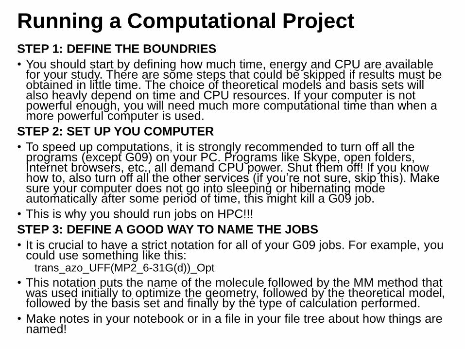
Running a Computational Project STEP 1: DEFINE THE BOUNDRIES

• You should start by defining how much time, energy and CPU are available for your study. There are some steps that could be skipped if results must be obtained in little time. The choice of theoretical models and basis sets will also heavly depend on time and CPU resources. If your computer is not powerful enough, you will need much more computational time than when a more powerful computer is used.

STEP 2: SET UP YOU COMPUTER

• To speed up computations, it is strongly recommended to turn off all the programs (except G09) on your PC. Programs like Skype, open folders, Internet browsers, etc., all demand CPU power. Shut them off! If you know how to, also turn off all the other services (if you’re not sure, skip this). Make sure your computer does not go into sleeping or hibernating mode automatically after some period of time, this might kill a G09 job.

• This is why you should run jobs on HPC!!!

STEP 3: DEFINE A GOOD WAY TO NAME THE JOBS

• It is crucial to have a strict notation for all of your G09 jobs. For example, you could use something like this:

trans_azo_UFF(MP2_6-31G(d))_Opt

• This notation puts the name of the molecule followed by the MM method that was used initially to optimize the geometry, followed by the theoretical model, followed by the basis set and finally by the type of calculation performed.

• Make notes in your notebook or in a file in your file tree about how things are named!

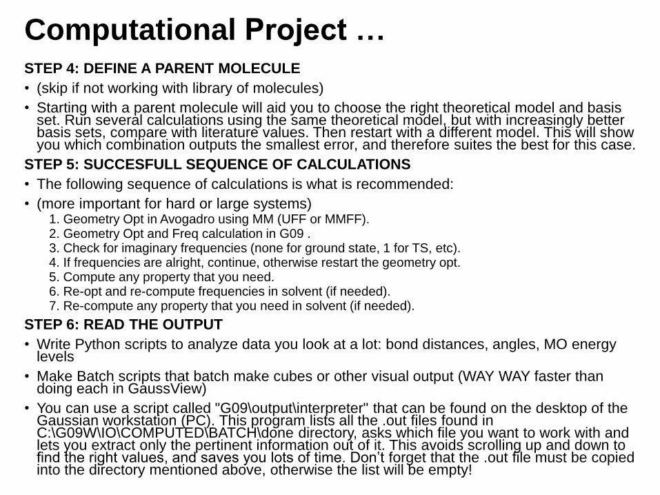
Computational Project …STEP 4: DEFINE A PARENT MOLECULE

• (skip if not working with library of molecules)

• Starting with a parent molecule will aid you to choose the right theoretical model and basis set. Run several calculations using the same theoretical model, but with increasingly better basis sets, compare with literature values. Then restart with a different model. This will show you which combination outputs the smallest error, and therefore suites the best for this case.

STEP 5: SUCCESFULL SEQUENCE OF CALCULATIONS

• The following sequence of calculations is what is recommended:

• (more important for hard or large systems)1. Geometry Opt in Avogadro using MM (UFF or MMFF).2. Geometry Opt and Freq calculation in G09 .3. Check for imaginary frequencies (none for ground state, 1 for TS, etc).4. If frequencies are alright, continue, otherwise restart the geometry opt.5. Compute any property that you need.6. Re-opt and re-compute frequencies in solvent (if needed).7. Re-compute any property that you need in solvent (if needed).

STEP 6: READ THE OUTPUT

• Write Python scripts to analyze data you look at a lot: bond distances, angles, MO energy levels

• Make Batch scripts that batch make cubes or other visual output (WAY WAY faster than doing each in GaussView)

• You can use a script called "G09\output\interpreter" that can be found on the desktop of the Gaussian workstation (PC). This program lists all the .out files found in C:\G09W\IO\COMPUTED\BATCH\done directory, asks which file you want to work with and lets you extract only the pertinent information out of it. This avoids scrolling up and down to find the right values, and saves you lots of time. Don’t forget that the .out file must be copied into the directory mentioned above, otherwise the list will be empty!