Embed Size (px)
Citation preview

1 COM INTRO: Interpolation © ECMWF 2014
Interpolation
Introduction and basic concepts
Computer User Training Course 2014
Peter Bispham
Development Section
2 COM INTRO: Interpolation © ECMWF 2014
Contents
Introduction
Overview of Interpolation
Spectral Transformations
Grid point Transformations
Interpolation Options
Future plans
Practical
3 COM INTRO: Interpolation © ECMWF 2014
Introduction
Weather data can have different representations
Interpolation is how we recalculate data in a different representation
Interpolation is available in
- MARS
- Operational dissemination
- Metview graphics package
Documentation:
https://software.ecmwf.int/emoslib
4 COM INTRO: Interpolation © ECMWF 2014
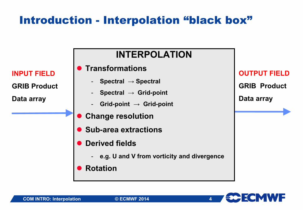
Introduction - Interpolation “black box”
INTERPOLATION
Transformations
- Spectral → Spectral
- Spectral → Grid-point
- Grid-point → Grid-point
Change resolution
Sub-area extractions
Derived fields
- e.g. U and V from vorticity and divergence
Rotation
INPUT FIELD
GRIB Product
Data array
OUTPUT FIELD
GRIB Product
Data array
5 COM INTRO: Interpolation © ECMWF 2014
Introduction – Interpolation black box (2)
Input can be a GRIB product or value array
Output can be a GRIB product or value array
For GRIB products, characteristics / info read from the GRIB header
A number of Fortran routines (part of EMOSLIB) perform the interpolation
MARS calls these for you
Possible to make calls to these functions yourself
Example programs on internet pages for EMOSLIB
6 COM INTRO: Interpolation © ECMWF 2014
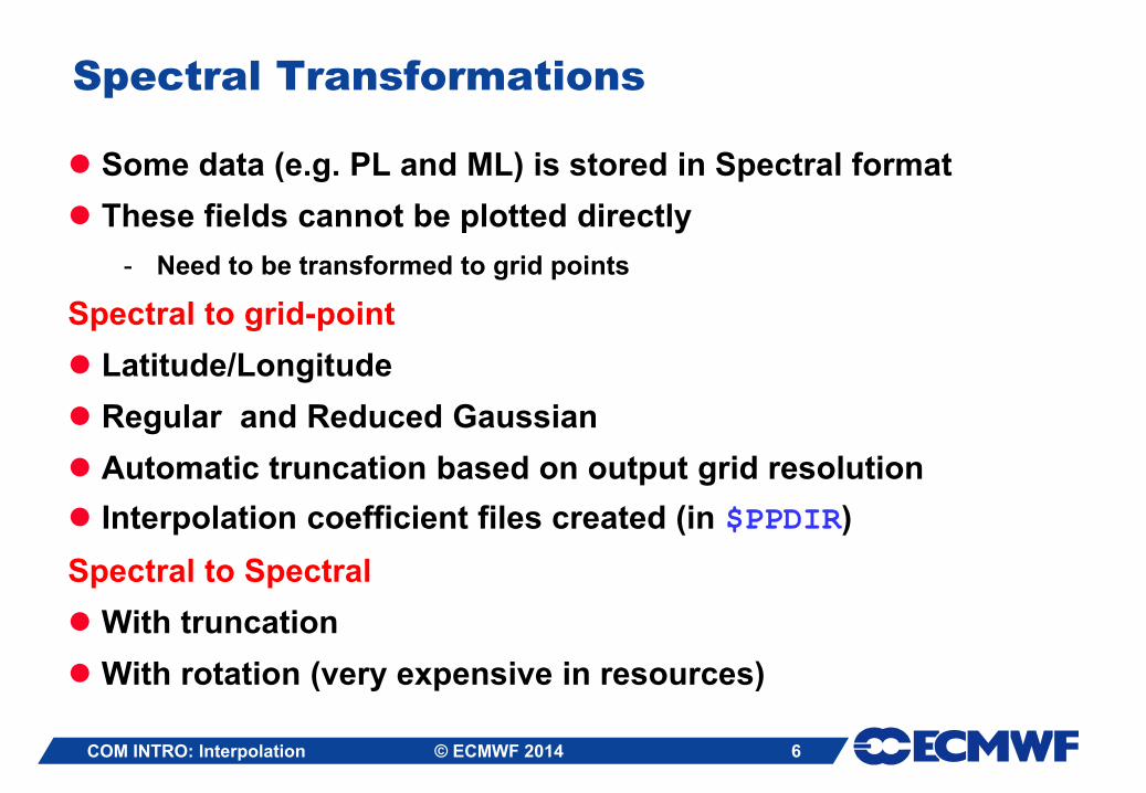
Spectral Transformations
Some data (e.g. PL and ML) is stored in Spectral format
These fields cannot be plotted directly
- Need to be transformed to grid points
Spectral to grid-point
Latitude/Longitude
Regular and Reduced Gaussian
Automatic truncation based on output grid resolution
Interpolation coefficient files created (in $PPDIR)
Spectral to Spectral
With truncation
With rotation (very expensive in resources)
7 COM INTRO: Interpolation © ECMWF 2014
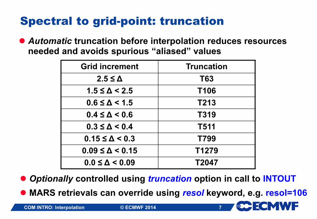
Spectral to grid-point: truncation
Automatic truncation before interpolation reduces resources needed and avoids spurious “aliased” values
Grid increment Truncation
2.5 ≤ Δ T63
1.5 ≤ Δ < 2.5 T106
0.6 ≤ Δ < 1.5 T213
0.4 ≤ Δ < 0.6 T319
0.3 ≤ Δ < 0.4 T511
0.15 ≤ Δ < 0.3 T799
0.09 ≤ Δ < 0.15 T1279
0.0 ≤ Δ < 0.09 T2047
Optionally controlled using truncation option in call to INTOUT
MARS retrievals can override using resol keyword, e.g. resol=106
8 COM INTRO: Interpolation © ECMWF 2014
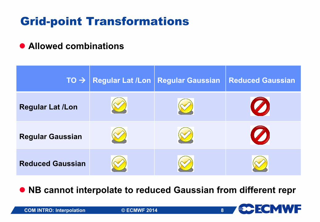
Grid-point Transformations
Allowed combinations
NB cannot interpolate to reduced Gaussian from different repr
TO
Regular Lat /Lon
Regular Gaussian
Reduced Gaussian
Regular Lat /Lon
Regular Gaussian
Reduced Gaussian

9 COM INTRO: Interpolation © ECMWF 2014
Regular Gaussian Grids
N lines of latitude between pole and equator
Latitude spacing not regular but is symmetric about equator
4 x N equally spaced points at each latitude
No latitude points at poles or equator
Special treatment at poles
N48
10 COM INTRO: Interpolation © ECMWF 2014
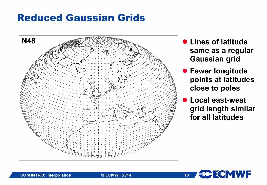
Reduced Gaussian Grids
Lines of latitude same as a regular Gaussian grid
Fewer longitude points at latitudes close to poles
Local east-west grid length similar for all latitudes
N48
11 COM INTRO: Interpolation © ECMWF 2014
Interpolation Options
These apply only to Grid-point Interpolation
Interpolation schemes
- Bilinear
- Nearest-neighbour
- 12-point scheme for rotation
Treatment of
- land-sea masks
- precipitation
Geographical sub-areas
12 COM INTRO: Interpolation © ECMWF 2014
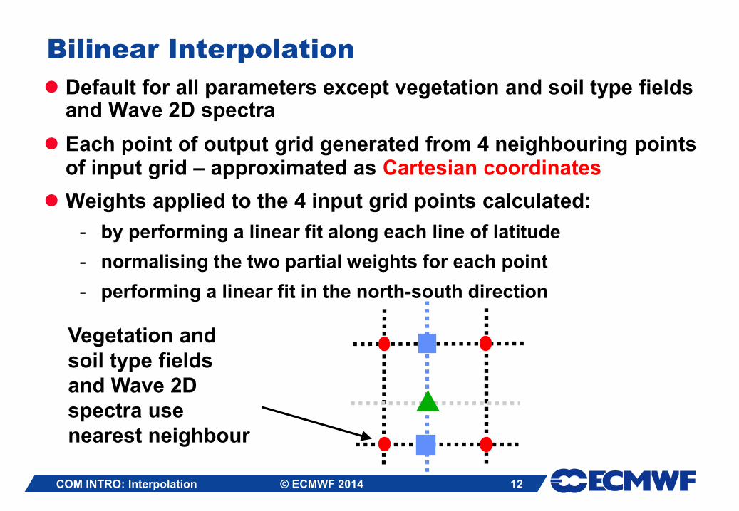
Bilinear Interpolation
Default for all parameters except vegetation and soil type fields and Wave 2D spectra
Each point of output grid generated from 4 neighbouring points of input grid – approximated as Cartesian coordinates
Weights applied to the 4 input grid points calculated:
- by performing a linear fit along each line of latitude
- normalising the two partial weights for each point
- performing a linear fit in the north-south direction
Vegetation and
soil type fields
and Wave 2D
spectra use
nearest neighbour
13 COM INTRO: Interpolation © ECMWF 2014
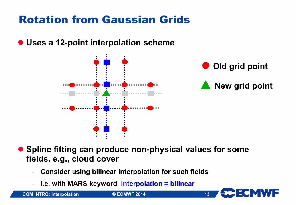
Rotation from Gaussian Grids
Uses a 12-point interpolation scheme
Old grid point
New grid point
Spline fitting can produce non-physical values for some fields, e.g., cloud cover
- Consider using bilinear interpolation for such fields
- i.e. with MARS keyword interpolation = bilinear
14 COM INTRO: Interpolation © ECMWF 2014
Land-Sea Masks
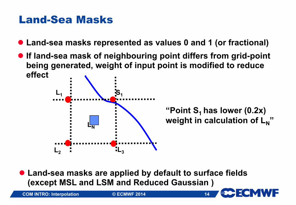
Land-sea masks represented as values 0 and 1 (or fractional)
If land-sea mask of neighbouring point differs from grid-point being generated, weight of input point is modified to reduce effect
Land-sea masks are applied by default to surface fields (except MSL and LSM and Reduced Gaussian )
“Point S1 has lower (0.2x)
weight in calculation of LN”
L1 S1
L2 L3
LN
15 COM INTRO: Interpolation © ECMWF 2014
Precipitation – an “accumulated field”
Rules are applied to prevent spreading of ‘trace’ amounts:
Interpolated value for precipitation at a point is set to zero if:
- the calculated value is less than a defined threshold
- its neighbour with the highest weight had no precipitation
Polar values for precipitation are always the average of nearest Gaussian line with no threshold check applied
For ensembles. accumulated fields can use “double” interpolation
- E.g. Interpolate from N320 to N160 and then to lat-lon
16 COM INTRO: Interpolation © ECMWF 2014
Geographical Sub-areas
Sub-areas can be created for new fields by specifying lat / lon boundaries (north / west / south / east)
Sub-areas are based on the full global grid
- Global regular grids have dateline at 0° West
- Lat/long grids have a line of latitude at the equator
- Gaussian grids are symmetrical about the equator
Boundaries of sub-areas are expanded outwards towards global grid (for rotations, boundaries are preserved)
- Can change behaviour in MARS by setting the environment variable
$MARS_INTERPOLATION_INWARDS
Sub-areas not currently supported for reduced Gaussian grids – full global grid is produced for these
17
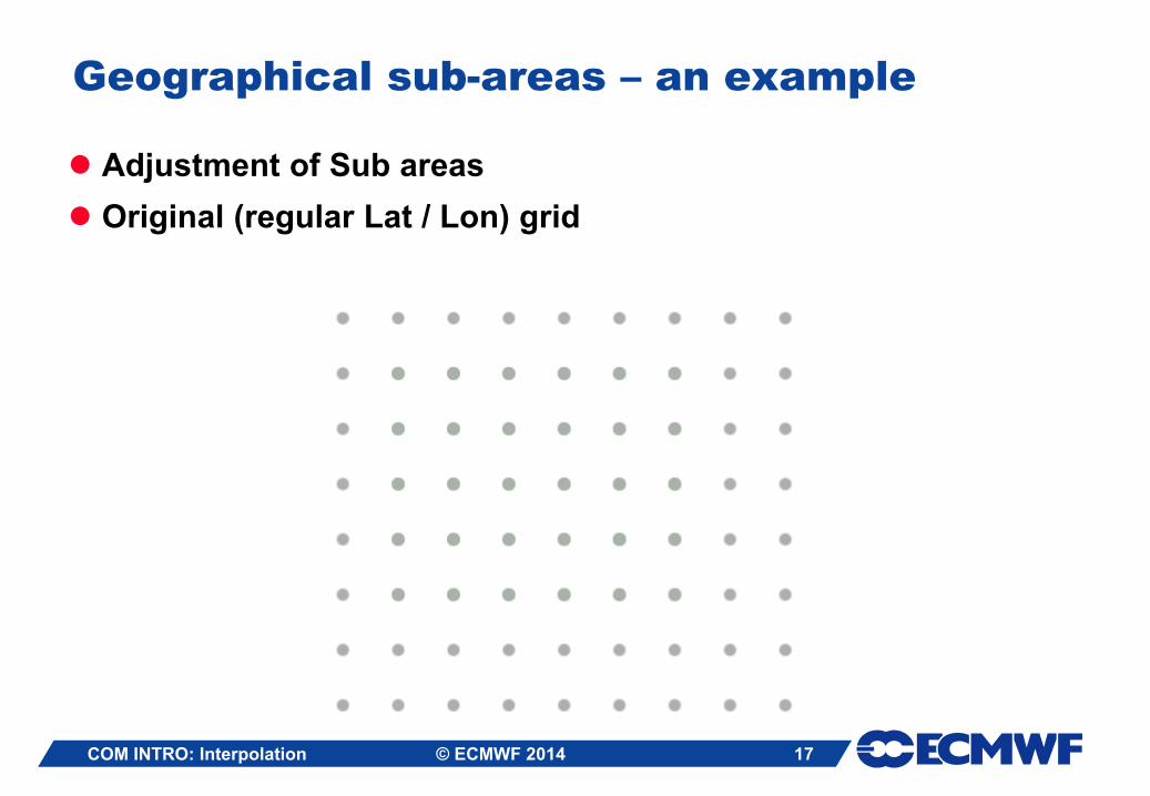
Geographical sub-areas – an example
Adjustment of Sub areas
Original (regular Lat / Lon) grid
COM INTRO: Interpolation © ECMWF 2014
18
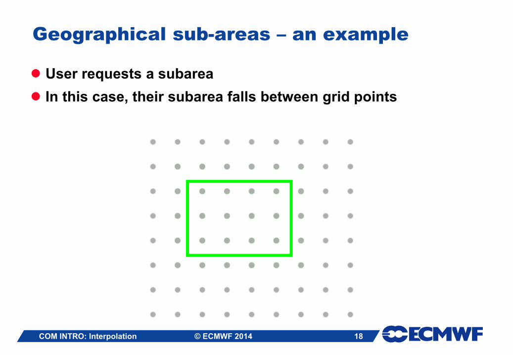
Geographical sub-areas – an example
User requests a subarea
In this case, their subarea falls between grid points
COM INTRO: Interpolation © ECMWF 2014
19
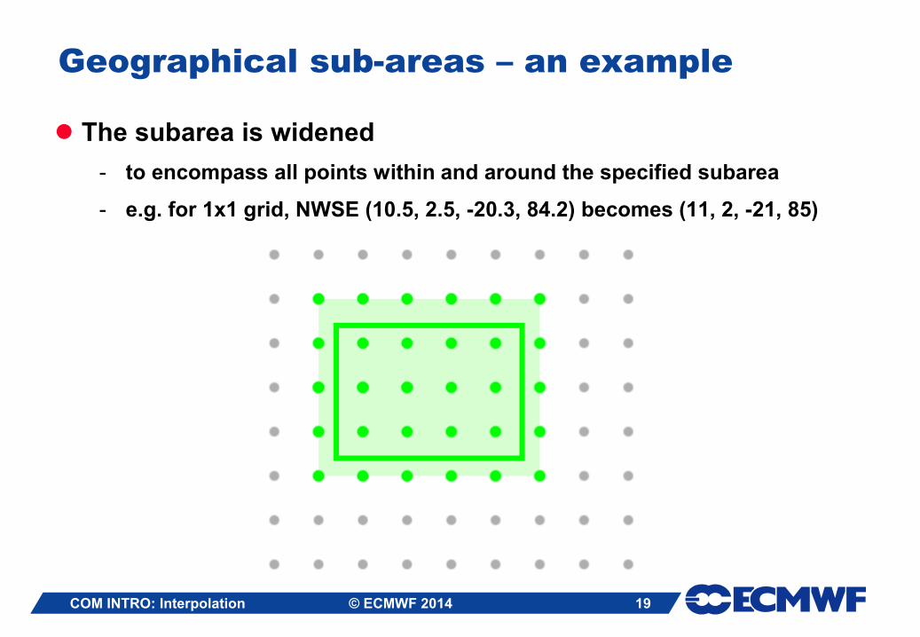
Geographical sub-areas – an example
The subarea is widened
- to encompass all points within and around the specified subarea
- e.g. for 1x1 grid, NWSE (10.5, 2.5, -20.3, 84.2) becomes (11, 2, -21, 85)
COM INTRO: Interpolation © ECMWF 2014
20
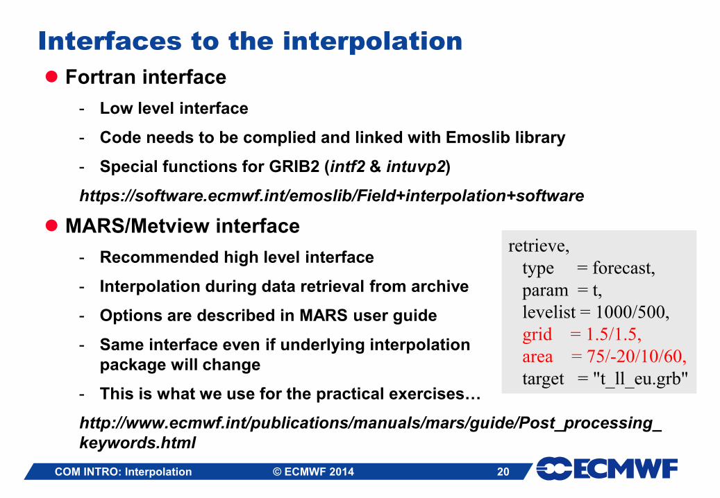
Interfaces to the interpolation
Fortran interface
- Low level interface
- Code needs to be complied and linked with Emoslib library
- Special functions for GRIB2 (intf2 & intuvp2)
https://software.ecmwf.int/emoslib/Field+interpolation+software
MARS/Metview interface
- Recommended high level interface
- Interpolation during data retrieval from archive
- Options are described in MARS user guide
- Same interface even if underlying interpolation
package will change
- This is what we use for the practical exercises…
http://www.ecmwf.int/publications/manuals/mars/guide/Post_processing_
keywords.html
COM INTRO: Interpolation © ECMWF 2014
retrieve,
type = forecast,
param = t,
levelist = 1000/500,
grid = 1.5/1.5,
area = 75/-20/10/60,
target = "t_ll_eu.grb"
21 COM INTRO: Interpolation © ECMWF 2014
Future plans
EMOSLIB is not easy to maintain
A new interpolation package is being written in C++
- Improve code, efficiency, maintainability and portability
The new package will provide a Library and API
- It will be callable from C, C++, Fortran 90, Python
- It will include some Unix-style command line tools
All current EMOSLIB features will be supported
Some new features will be added
- Include routines for ‘single-point’ interpolation
- Handle different grid types
- Parallelisation / multiple-threaded
Will undergo extensive testing at ECMWF before release
22
Practical: Interpolation with MARS
Work in your $SCRATCH
Copy the scripts from ~trx/maf/scripts
cd $SCRATCH
cp /home/ectrain/trx/maf/scripts/interp*.ksh ./
First, run interp1.ksh:
./interp1.ksh
This will retrieve some data from MARS to a file out1.grib
Next run the other scripts in turn. Each will create a new file called out2.grib, … , out7.grib
Inspect each output file with grib_ls and grib_dump
- Note how the grid description in Section 2 of the header differs
- Look at the MARS requests that create each of the files
COM INTRO: Interpolation © ECMWF 2014


