Technical Memo - ECMWF

ical Memo Technical Memo Technical Memo Technical Memo Technnical Memo Technical Memo Technical Memo Technical Memo Technical Memo Technical Memo Technical Memo Technical Memo Te

Technical Memo Technical Memo Technical Memo Technical Memo Technical Memo Technical Memo Technical Memo Technical Technical Memo Technical Memo Technical Memo Technical Memo Technical Memo Technical Memo Technical Memo Technical










Technical Memo Technical Memo Technical Memo Technical Memo Technical Memo Technical Memo Technical Memo Technical

TechnicalMemo

890Notes on shallow water extension of Miles Theory

Peter A.E.M. JanssenJanuary 2022

Series: ECMWF Technical Memoranda

A full list of ECMWF Publications can be found on our website under: http://www.ecmwf.int/en/publications

Contact: [email protected]

© Copyright 2022

European Centre for Medium-Range Weather Forecasts, Shinfield Park, Reading, RG2 9AX, UK

Literary and scientific copyrights belong to ECMWF and are reserved in all countries. The content of this document is available for use under a Creative Commons Attribution 4.0 International Public License. See the terms at https://creativecommons.org/licenses/by/4.0/.

The information within this publication is given in good faith and considered to be true, but ECMWF accepts no liability for error or omission or for loss or damage arising from its use.

http://www.ecmwf.int/en/publications

mailto:library%40ecmwf.int?subject=

https://creativecommons.org/licenses/by/4.0/

Notes on shallow water extension of Miles Theory

Abstract

We present results from a straightforward extension of Miles’ theory of wind-wave generation to-

wards shallow water. Both numerical results and an approximate analytical expression for the

growthrate are obtained. The analytical expression forms the basis for a parametrization of wind

wave growth in numerical wave prediction models.

The present wind input term in third generation models is based on the assumption that the wind-

wave generation depends, regarding ocean wave properties, only on the phase speed of the waves. In

this work it is shown that for the short waves (kD > 1, with k the wavenumber and D the local depth)

this is indeed a good assumption, but for the long waves, with kD << 1, there will be an overestimate

of wind input. Nevertheless, simulations with the energy balance equation for the duration limited

case show that the present wind input term and the newly proposed windinput term give almost iden-

tical evolution of wave height and spectrum. This may be understood by noting that in equilibrium

conditions kpD ≃ 1 (with kp the peak wavenumber), in other words in practical circumstances waves

are short enough so that the difference between present and new wind input source function does not

matter.

1 Introduction

In the mid 1980’s Gerbrand Komen, Gao Quanduo and myself worked on the first version of the shallow

water extension of the WAM model. One of the topics was, of course, to find an appropiate expression

for the wind input source function. I extended Miles theory towards shallow water and we found that in

a good approximation even in shallow water the wind input term may be parametrized in terms of the

dimensionless phase speed c/u∗ where c is the phase speed of the wave and u∗ is the friction velocity in

air. At least, the approximation was found to be adequate for fairly short waves with kD > 1. The reason

that this approach works so well has to do with the fact that according to Miles theory the growthrate

of the waves by wind is to a large extent determined by the curvature in the wind profile at the critical

height zc. Here, the critical height is determined by the condition that the wind speed U0(z) at zc matches

the phase speed of the surface gravity wave of interest: The condition U0(zc)−c = 0 expresses that there

is a resonant interaction between the airflow around z = zc and the wave with phase speed c.

In 2012 I received a preliminary version of the paper of Montalvo et al. (2013) in which it was reported

that there are considerable deviations from the WAM parametrization of the wind input source function.

As I have lost all my notes on this subject it was decided to redo the original work in order to see whether

the results from Montalvo et al. (2013) could be reconciled with the earlier results Gerbrand Komen and

I found.

The programme of this note is therefore as follows. In §2 I extend Miles’ theory towards shallow water

waves and I discuss the differences with deep water theory. This is followed in §3 by a discussion of

the numerical results and a derivation of an approximate solution, originally derived by Miles (1993) for

deep water. However, Miles was fairly economical with the details of this derivation and therefore the

full details are presented in the Appendix. The approximate expression for the wave growth is valid for

small dimensionless critical height µ = k(zc+z0) only, where zc is the critical height and z0 the roughness

length. As argued in §4, in deep water growth rates of the waves are underestimated for the long waves

and therefore parameters in the approximate expression have been rescaled to match observed growth

rates. This then gives the parametrization of wave growth that has been used for many years in the WAM

model. This parametrization was designed in such a way that even in shallow water the growth rate only

depends on the dimensionless phase speed c/u∗. However, in the present work the results of Montalvo

et al. (2013) will be confirmed who showed that for really long waves with kD << 1 this approach

Technical Memorandum No. 890 1


is not adequate. Nevertheless, the approximate expression for the wave growth is still fine when the

appropriate definition of the critical height in shallow water is used and when appropriate shallow water

effects are taken into account. Unfortunately, in practice it turns out that simulations with the energy

balance equation for the duration limited case show that the present wind input term and the newly

proposed windinput term give almost identical evolution of wave height and spectrum. This is easily

understood when it is realized that in equilibrium windsea conditions kpD ≃ 1.

Nevertheless, in extreme circumstances there could be differences between the new and old approach,

and since the new approach is physically more sound the resulting shallow water formulation was imple-

mented in CY40R1 (November 2013).

2 Miles theory and shallow water effects.

The starting point is the treatment of Miles theory by Janssen (2004). Here, air and water are treated as

one fluid. Growth rates of the waves by wind follow from the question under what conditions there is

instability of the equilibrium

u0 =U0(z)ex, g =−gez,

ρ0 = ρ(z), p0(z) =−g

∫

dz ρ0(z), (1)

where ex and ez are unit vectors in the x- and z-direction. Thus, we deal with a plane parallel flow whose

speed U0 and density ρ0 only depends on height z.

In order to answer this question one uses the equations for an adiabatic fluid with an infinite sound speed

and one linearizes these equations around the above equilibrium condition. For normal modes of the

form w = wei(kx−ωt), where in this case w is the vertical velocity, k is the wavenumber and ω is the

unknown angular frequency, one finds the following Sturm-Liouville problem for the displacement of

the streamlines ψ = w/W ,

d

dz

(

ρ0W 2 d

dzψ

)

−(

k2ρ0W 2 +gρ ′0

)

ψ = 0. (2)

Here, W =U0−c, with c = ω/k the phase speed of the waves and the prime denotes differentiation of an

equilibrium quantity with respect to height z. The prominent role of the critical layer is evident through

the Doppler-shifted velocity W . The equation for the perturbed streamlines is subject to the boundary

condition of vanishing displacement at infinite height and at finite depth D,

ψ → 0, z → ∞

ψ(z =−D) = 0. (3)

The boundary value problem (2)-(3) determines, in principle, the real and imaginary part of the complex

phase speed c = ω/k, giving the growth rate γ = ℑ(ω) of the waves.

Whether there is instability or not can only be decided by solving the boundary value problem. This

will be done for the special case of surface gravity waves. This case follows by choosing an appropriate

density profile, i.e. the density profile is chosen constant in air and water with a jump at the interface at

z = 0. As the air density ρa is much smaller than the water density ρw, there is a small parameter s =ρa/ρw ≈ 10−3 in the problem allowing to construct an approximate solution of the eigenvalue problem

(2)-(3).

2 Technical Memorandum No. 890


In water we assume that effects of the current may be neglected and that the water density is a constant,

hence (2) becomes for z < 0

d2

dz2ψw = k2ψw, (4)

and with the boundary condition ψ(z =−D) = 0 the solution becomes

ψw = ψ0

sinhk(z+D)

sinhkD, (5)

where ψ0 is arbitrary. At the air-sea interface the boundary condition is now that ψ be continuous. The

second condition follows from an integration of (2) from just below the surface, z =−0, to just above the

surface, z = +0. Note that at z = 0 the density profile shows a jump so that ρ ′0 = (ρa −ρw)δ (z) where

δ (z) is the Dirac delta function. The result is

ρ0W 2 d

dzψ

∣

∣

∣

∣

+0

−0

=∫ +0

−0dz[

ρ0k2W 2 +gρ ′0

]

ψ . (6)

Since in the limit only the integral involving ρ ′0 gives a contribution, we obtain, using (5), the following

dispersion relation for the phase speed of the waves

c2

c20

=(1− s)

1− sZψ ′a(0)/k

, s =ρa

ρw

, Z =ω2

0

gk, (7)

with ω20 = gk tanhkD the dispersion relation for free gravity waves in shallow water while c0 is the

corresponding phase speed of the waves. Furthermore, without loss of generality, we have taken the

amplitude ψ0 = 1 as we are dealing with a linear problem. Once the vertical gradient of the displacement

of the streamlines in the air (i.e. ψ ′a(0)) is known we can establish the growth rate of the waves. This

follows in principle from the application of (2)-(3) to the air. Taking a constant air density one finds for

ψa the simplified problem

d

dz

(

W 2 d

dzψa

)

= k2W 2ψa,

ψa(0) = 1; (8)

ψa → 0, z → ∞.

Here, W = U0(z)− c is still unknown as c follows from Eq. (7), which shows that the phase speed c

depends on the solution ψa but this dependence is weak as the density ratio s is small. In other words, in

the absence of air the usual dispersion relation for free gravity waves, i.e. c2 = c20, follows. The effect of

air on the surface gravity waves is small since s ≪ 1 and therefore the dispersion relation can be solved

in an approximate manner with the result

c = c0 + sc1 + ...., (9)

with c20 = g tanhkD/k and c1 =

12c0(Zψ ′

a/k−1). As a result, the problem (8) now reduces to

d

dz

(

W 20

d

dzψa

)

= k2W 20 ψa,

ψa(0) = 1, (10)

ψa → 0, z → ∞.



where W0 = U0 − c0 is now known, and as a consequence the solution to the differential equation is

simplified considerably. However, the limit of vanishing c1 in the expression for the Doppler-shifted

velocity has to be taking with care, in particular when integrating expressions involving the inverse of

W0. This is discussed in more detail in Janssen (2004), and as a rule, for growing solutions, the integration

contour needs to be indented below the singularity. In addition, we now have an explicit expression for

the growth rate γa of the amplitude of the waves. With ℑ the imaginary part we find

γa

ω0

= sℑ

(

c1

c0

)

=sZ(kD)

2kℑ(ψ ′

a) =sZ(kD)

4kW (ψa,ψ

∗a )

∣

∣

∣

∣

z=0

(11)

where the Wronskian W is given by

W (ψa,ψ∗a ) =−i

(

ψ ′aψ∗

a −ψaψ ′∗a

)

. (12)

As discussed in Janssen (2004) the Wronskian has a physical interpretation as it is directly connected to

the wave-induced stress τw,

τw =−〈δuδw〉=− i

k

(

w∗w′−ww′∗)=W 2

kW (ψa,ψ

∗a ). (13)

In summary, in order to obtain the growthrate of waves by wind one needs to solve the boundary value

problem (10) and then ψ ′a is used in (11) which then immediately gives the growthrate γa. Before in the

next Section two possible methods of solving the differential equation (10) are discussed, we mention

here that shallow water effects enter the problem in two ways. The first one is through the factor Z =ω2

0/gk in the expression for the growth rate. Clearly, when Z is smaller than 1 there are deviations from

the deep-water dispersion relation. In fact, in the shallow water limit kD → 0 one finds that Z → kD.

Hence, for shallow water waves the growthrate of the waves by wind is expected to become small,

provided the displacement of the streamlines in air remains finite in the shallow water limit.

Shallow water effects also occur through the Doppler-shifted velocity W0 =U0−c0. Whilst in deep water

the phase speed is ever increasing with decreasing wavenumber, in sharp contrast to this, in shallow

water the phase speed c0 reaches a maximum given by cmax0 =

√gD for very long waves. This will

have a pronounced impact on the magnitude of the critical height and on the growth rate, which will

increase as explained in the next Section. However, combining now the two effects it turns out that the

depth dependence of Z is overwhelming with the result that for the same wavenumber the growthrate of

shallow water waves is smaller than the corresponding growth rate for deep water, while in the limit of

shallow water waves the growth rate vanishes. This will be discussed in more detail in the next section.

3 Numerical and analytical solution.

Before we present numerical and analytical results, it is remarked that it is rather common to use the

vertical component of the wave-induced velocity instead of the displacement of the streamlines ψ ∼w/W . In terms of the normalised vertical velocity χ = w/w(0), the eigenvalue problem (10) becomes

W0

(

d2

dz2− k2

)

χ =W ′′0 χ,

χ(0) = 1, (14)

χ → 0, z → ∞.



and the growth rate of the wave is given by

γa

sω0

=Z(kD)

4kW (χ,χ∗)

∣

∣

∣

∣

z=0

, (15)

where the Wronskian is now given by W =−i(χ ′χ∗−χχ ′∗).

Regarding (14) we remark that the differential equation, known as the Rayleigh equation, has a singular-

ity at W0 =U0 −c0 = 0. Since W0 = 0 defines the critical height zc (i.e. the height where the phase speed

of the wave matches the wind speed) it is now clear that the resonance at the critical height plays a special

role in the problem of wind-wave generation. The role of the critical height becomes even clearer when

the Wronskian W is evaluated. By means of the Rayleigh equation it may be shown that the Wronskian

is independent of height except at the critical height where it may show a jump. Explicitely one finds

that for z > zc the Wronskian vanishes while for z < zc one finds

W =−2πW ′′

0c

|W ′0c |

| χc |2,

and therefore the growth rate of the waves becomes

γa

sω0

=−πZ(kD)

2k

W ′′0c

|W ′0c |

| χc |2 . (16)

This is Miles’ classical result for the growth of surface gravity waves due to shear flow. From (16) we

obtain the well-known result that only those waves are unstable for which the curvature W ′′0 =U ′′

0 of the

wind profile at the critical height is negative. This is the case, for example, for a logarithmic profile.

Therefore, the critical height zc plays a key role in the problem of the generation of ocean waves by wind

as the air at zc height enjoys a resonant interaction with the gravity wave with phase speed c.

In order to solve the boundary value problem (14), we finally have to specify the shape of the wind

profile. In case of neutrally stable conditions (no density stratification by heat and moisture) the wind

profile has a logarithmic height dependence. Hence,

U0(z) =u∗κ

log(1+ z/z0), (17)

which follows from the condition that the momentum flux in the surface layer is a constant for steady

conditions. Recall that κ = 0.40 is the von Karman constant which is supposed to be a universal constant,

the friction velocity u∗ is a measure for the momentum flux in the surface layer and the roughness length

z0 is a parameter which reflects the momentum loss at the sea surface. It is given by the Charnock relation

z0 = αCHu2∗/g, (18)

with αCH the Charnock parameter. Although in the present linear treatment it is assumed that the

Charnock parameter αCH is a constant 1, there are arguments why αCH is not a constant but depends

on the sea state.

For given wind profile (17) the boundary value problem (14) may now be solved. Originally, Miles

(1957) applied a variational approach to obtain an approximate solution. However, when compared to

the numerical results of Conte and Miles (1959) this approximation gave growth rates which were too

large by a factor of three. Prompted by asymptotic matching results of van Duin and Janssen (1992),

Miles (1993) revisited this problem and realized that the overestimation was caused by the neglect of

1we take αCH = 0.0144, because this was the typical value in the bight of Abaco experiment of Snyder et al. (1981).



some higher order terms. The improved approximation gave good agreement with Conte and Miles

(1959). However, the approximation of Miles (1993) is formally only valid for ’slow’ waves which have

a small critical height. This will be illustrated by comparing the results of the Miles approximation with

the numerical results. Furthermore, we study shallow water effects on the growth rate of the waves by

wind and we extend the range of validity of the Miles’ approximation towards shallow water.

3.1 numerical results.

Before we discuss the numerical results of the growth rate, dimensionless quantities are introduced in

order to see which parameters determine the problem. This scaling behaviour can be achieved in several

manners and we discuss two of them, one in the context of the numerical solution and one in the context

of the approximate solution.

Since we are dealing with gravity waves it is natural to use the acceleration of gravity g as a basic scaling

quantity. Judging from the equilibrium form of the wind profile (17) the other basic scaling quantity is

the friction velocity u∗. Thus, we scale velocities with u∗ and in agreement with the Charnock relation

(18) lengths scale with u2∗/g, hence

z∗ = gz/u2∗,z0∗ = gz0/u2

∗,D∗ = gD/u2∗

c∗ = c/u∗,U0∗ =U0/u∗, (19a)

while the dimensionless wavenumber becomes

k∗ = ku2∗/g. (19b)

As a consequence, the boundary value problem (14) has in terms of these dimensionless quantities the

same form, while from (17)- (18) the dimensionless wind profile becomes

U0∗ =1

κlog(1+

z∗z0∗

). (20)

For a given wave characterized by its dimensionless phase speed c∗ we can solve for the dimensionless

growth rate γ/ω0 of the energy of the waves, which is twice the growth rate of the amplitude of the

waves,

γ/ω0 = 2γa/ω0. (21)

The dimensionless growth rate depends in general on the dimensionless phase speed c∗ and on two

dimensionless parameters, namely the dimensionless roughness length z0∗ and the dimensionless depth

parameter D∗. However, remarkably, with Charnock’s relation we have z0∗ = αCH which for the moment

is regarded as a constant, independent of u∗ and of sea state. Therefore, for a neutrally stable airflow

with a logarithmic wind profile, the growth rate γ/ω0 only depends on c∗ and on the parameter D∗.

Following scaling arguments of Miles (1957) the growth rate of the waves can be written in the general

form

γ/ω0 = sβu2∗

c2, (22)

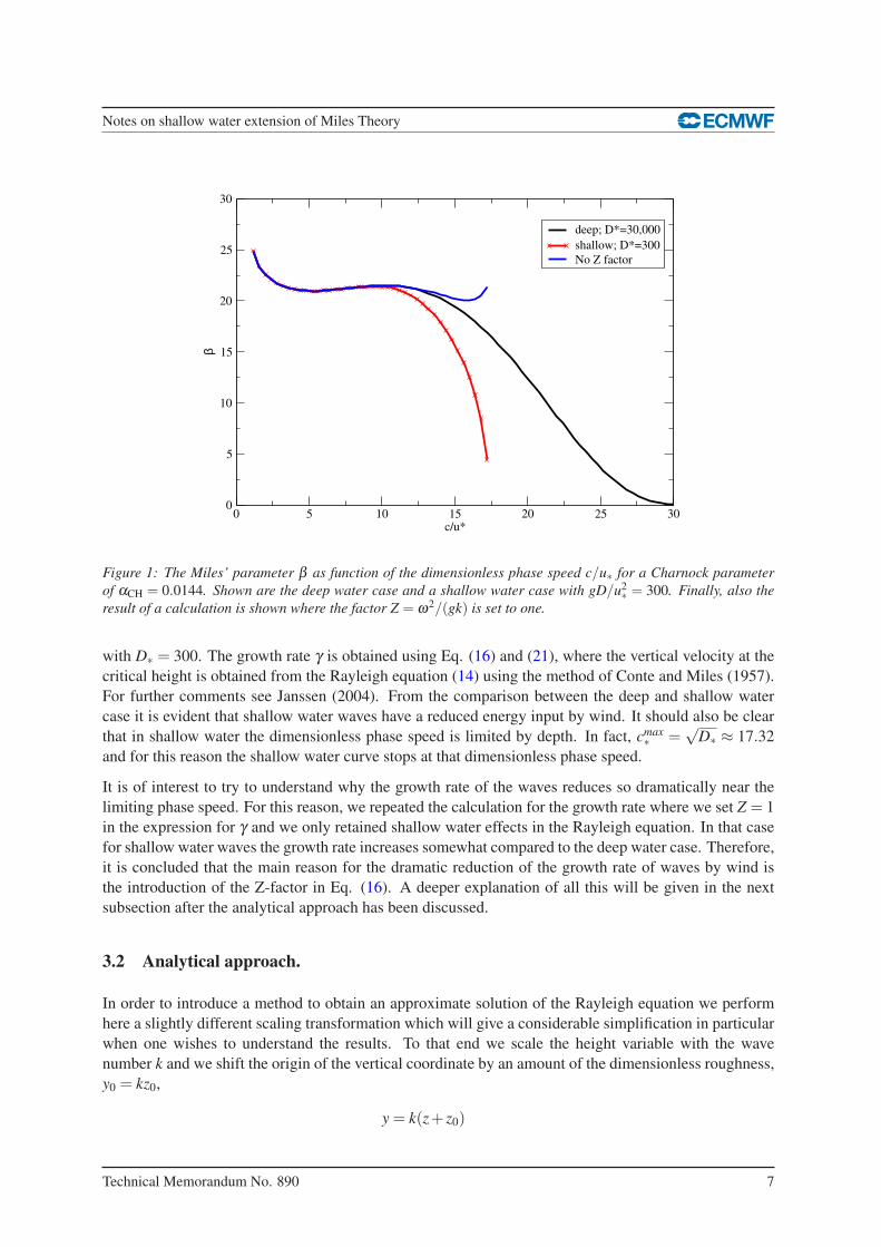
where β is the so-called Miles parameter. In Fig. 1 a plot is shown of the Miles parameter as function

of the dimensionless phase speed c/u∗ for the deep water case (D∗ = 30,000) and a shallow water case



0 5 10 15 20 25 30c/u*

0

5

10

15

20

25

30β

deep; D*=30,000

shallow; D*=300

No Z factor

Figure 1: The Miles’ parameter β as function of the dimensionless phase speed c/u∗ for a Charnock parameter

of αCH = 0.0144. Shown are the deep water case and a shallow water case with gD/u2∗ = 300. Finally, also the

result of a calculation is shown where the factor Z = ω2/(gk) is set to one.

with D∗ = 300. The growth rate γ is obtained using Eq. (16) and (21), where the vertical velocity at the

critical height is obtained from the Rayleigh equation (14) using the method of Conte and Miles (1957).

For further comments see Janssen (2004). From the comparison between the deep and shallow water

case it is evident that shallow water waves have a reduced energy input by wind. It should also be clear

that in shallow water the dimensionless phase speed is limited by depth. In fact, cmax∗ =

√D∗ ≈ 17.32

and for this reason the shallow water curve stops at that dimensionless phase speed.

It is of interest to try to understand why the growth rate of the waves reduces so dramatically near the

limiting phase speed. For this reason, we repeated the calculation for the growth rate where we set Z = 1

in the expression for γ and we only retained shallow water effects in the Rayleigh equation. In that case

for shallow water waves the growth rate increases somewhat compared to the deep water case. Therefore,

it is concluded that the main reason for the dramatic reduction of the growth rate of waves by wind is

the introduction of the Z-factor in Eq. (16). A deeper explanation of all this will be given in the next

subsection after the analytical approach has been discussed.

3.2 Analytical approach.

In order to introduce a method to obtain an approximate solution of the Rayleigh equation we perform

here a slightly different scaling transformation which will give a considerable simplification in particular

when one wishes to understand the results. To that end we scale the height variable with the wave

number k and we shift the origin of the vertical coordinate by an amount of the dimensionless roughness,

y0 = kz0,

y = k(z+ z0)



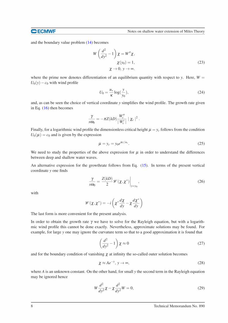
and the boundary value problem (14) becomes

W

(

d2

dy2−1

)

χ =W ′′χ,

χ(y0) = 1, (23)

χ → 0, y → ∞.

where the prime now denotes differentiation of an equilibrium quantity with respect to y. Here, W =U0(y)− c0 with wind profile

U0 =u∗κ

log(y

y0

), (24)

and, as can be seen the choice of vertical coordinate y simplifies the wind profile. The growth rate given

in Eq. (16) then becomes

γ

sω0

=−πZ(kD)W ′′

c

|W ′c |

| χc |2 .

Finally, for a logarithmic wind profile the dimensionless critical height µ = yc follows from the condition

U0(µ) = c0 and is given by the expression

µ = yc = y0eκc/u∗ . (25)

We need to study the properties of the above expression for µ in order to understand the differences

between deep and shallow water waves.

An alternative expression for the growthrate follows from Eq. (15). In terms of the present vertical

coordinate y one finds

γ

sω0

=Z(kD)

2W (χ,χ∗)

∣

∣

∣

∣

y=y0

, (26)

with

W (χ,χ∗) =−i

(

χ∗ dχ

dy−χ

dχ∗

dy

)

The last form is more convenient for the present analysis.

In order to obtain the growth rate γ we have to solve for the Rayleigh equation, but with a logarith-

mic wind profile this cannot be done exactly. Nevertheless, approximate solutions may be found. For

example, for large y one may ignore the curvature term so that to a good approximation it is found that

(

d2

dy2−1

)

χ ≈ 0 (27)

and for the boundary condition of vanishing χ at infinity the so-called outer solution becomes

χ ≈ Ae−y, y → ∞, (28)

where A is an unknown constant. On the other hand, for small y the second term in the Rayleigh equation

may be ignored hence

Wd2

dy2χ −χ

d2

dy2W = 0, (29)



which has the general solution

χ ≈ aW

(

1+b

∫ y

y0

dη

W 2(η)

)

, (30)

where a and b are obtained from the boundary conditions. The above solution which holds for small

y is called the inner solution. Then, the constant a immediately follows from the boundary condition

χ(y0) = 1, hence a = 1/W (y0). However, it is not straightforward to determine the constant b from the

boundary condition at infinity. One reason is that the solution (30) is only valid for small y, while the

solution (28) is valid for large y. Another reason is that formally the second independent solution of (30)

has a singularity and a branch cut needs to be introduced in order to make it single-valued.

In the Appendix it is shown how by means of the method of asymptotic matching the parameter b may

be obtained. Basically, the small y limit of the outer solution (28) is matched to the large y limit of the

inner solution (30) resulting in algebraic equations for A, a and b. As a result one finds

b =− u2∗

κ2log2

(yc

λ

) 1

1+ iΓ, (31)

where

Γ = πyc log2(yc

λ

)

, and λ =1

2e−γE ≈ 0.281, (32)

with γE = 0.5771 Euler’s constant.

It is emphasized that this solution has a restricted validity because it is assumed that the inner region,

with y = O(yc), and outer region, with y = O(1), are distinct. This can only be achieved if yc ≪ 1. In

deep water, therefore, where yc increases for increasing phase speed the above approximation is expected

to fail. In shallow water where there is a limiting phase speed this needs not to be the case and the above

solution with b given by Eq. (31) works remarkably well as will be seen in a moment.

Now, in order to evaluate the growth rate the Wronskian W is required. Using Eq. (30) one finds

W =2π

κ2yc log4

(yc

λ

) u2∗

c2(33)

and the analytical expression for the growth rate follows at once by substituting (33) into (26),

γ/ω0 = sβu2∗

c2, β =

π

κ2Z(kD)yc log4

(yc

λ

)

,yc ≤ λ . (34)

In deep water this result agrees with Miles (1993).

Let us compare the analytical approximation with the numerical results for deep and shallow water. In

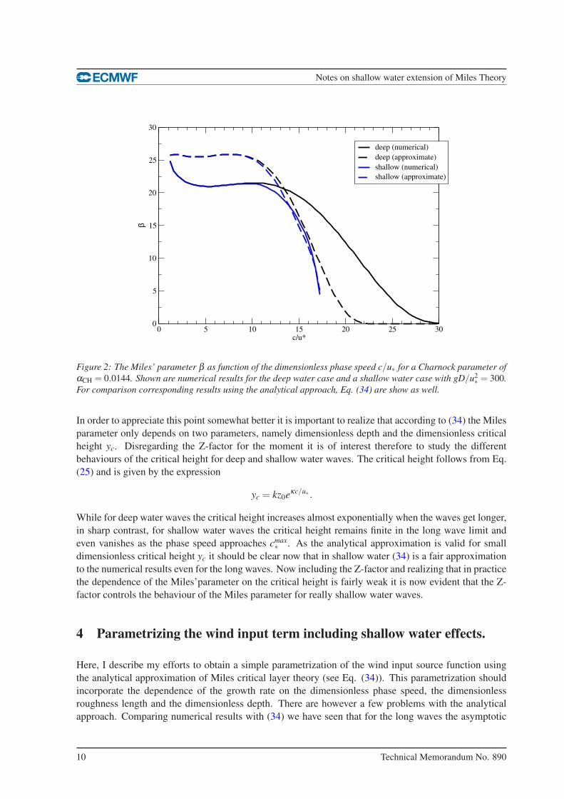
Fig. 2 the Miles’ parameter β is plotted as function of the dimensionless phase speed c/u∗ for a Charnock

parameter of αCH = 0.0144. Shown are numerical results for the deep water case and a shallow water

case with gD/u2∗ = 300. For comparison corresponding results using the analytical approach, Eq. (34)

are show as well. Considering the deep water case first, it is clear that the analytical result (34) is a fair

approximation to the numerical results 2 for the slow waves, but for the fast, long waves, which have

a dimensionless critical height of the order 1, the analytical result clearly fails. On the other hand, in

shallow water, the agreement between numerical results and (34) is much more impressive.

2in particular realizing that the original approximation by Miles (1957) was off by a factor of 3. The present improvement is

entirely caused by the factor λ in the log term of (34). The λ factor follows from higher order matching as explained in detail

in the Appendix.



0 5 10 15 20 25 30c/u*

0

5

10

15

20

25

30

βdeep (numerical)

deep (approximate)

shallow (numerical)

shallow (approximate)

Figure 2: The Miles’ parameter β as function of the dimensionless phase speed c/u∗ for a Charnock parameter of

αCH = 0.0144. Shown are numerical results for the deep water case and a shallow water case with gD/u2∗ = 300.

For comparison corresponding results using the analytical approach, Eq. (34) are show as well.

In order to appreciate this point somewhat better it is important to realize that according to (34) the Miles

parameter only depends on two parameters, namely dimensionless depth and the dimensionless critical

height yc. Disregarding the Z-factor for the moment it is of interest therefore to study the different

behaviours of the critical height for deep and shallow water waves. The critical height follows from Eq.

(25) and is given by the expression

yc = kz0eκc/u∗ .

While for deep water waves the critical height increases almost exponentially when the waves get longer,

in sharp contrast, for shallow water waves the critical height remains finite in the long wave limit and

even vanishes as the phase speed approaches cmax∗ . As the analytical approximation is valid for small

dimensionless critical height yc it should be clear now that in shallow water (34) is a fair approximation

to the numerical results even for the long waves. Now including the Z-factor and realizing that in practice

the dependence of the Miles’parameter on the critical height is fairly weak it is now evident that the Z-

factor controls the behaviour of the Miles parameter for really shallow water waves.

4 Parametrizing the wind input term including shallow water effects.

Here, I describe my efforts to obtain a simple parametrization of the wind input source function using

the analytical approximation of Miles critical layer theory (see Eq. (34)). This parametrization should

incorporate the dependence of the growth rate on the dimensionless phase speed, the dimensionless

roughness length and the dimensionless depth. There are however a few problems with the analytical

approach. Comparing numerical results with (34) we have seen that for the long waves the asymptotic



0 5 10 15 20 25 30c/u*

0

10

20

30

40

50β

Miles Theory

ParametrizationSnyder et al (long waves)

Plant and Wright (short waves)

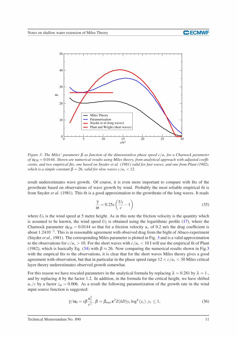
Figure 3: The Miles’ parameter β as function of the dimensionless phase speed c/u∗ for a Charnock parameter

of αCH = 0.0144. Shown are numerical results using Miles theory, from analytical approach with adjusted coeffi-

cients, and two empirical fits, one based on Snyder et al. (1981) valid for fast waves, and one from Plant (1982),

which is a simple constant β = 26, valid for slow waves c/u∗ < 12.

result underestimates wave growth. Of course, it is even more important to compare with fits of the

growthrate based on observations of wave growth by wind. Probably the most reliable empirical fit is

from Snyder et al. (1981). This fit is a good approximation to the growthrate of the long waves. It reads

γ

ω= 0.25s

(

U5

c−1

)

(35)

where U5 is the wind speed at 5 metre height. As in this note the friction velocity is the quantity which

is assumed to be known, the wind speed U5 is obtained using the logarithmic profile (17), where the

Charnock parameter αCH = 0.0144 so that for a friction velocity u∗ of 0.2 m/s the drag coefficient is

about 1.2410−3. This is in reasonable agreement with observed drag from the bight of Abaco experiment

(Snyder et al., 1981). The corresponding Miles parameter is plotted in Fig. 3 and is a valid approximation

to the observations for c/u∗ > 10. For the short waves with c/u∗ < 10 I will use the empirical fit of Plant

(1982), which is basically Eq. (34) with β ≈ 26. Now comparing the numerical results shown in Fig.3

with the emprical fits to the observations, it is clear that for the short waves Miles theory gives a good

agreement with observation, but that in particular in the phase speed range 12 < c/u∗ < 30 Miles critical

layer theory underestimates observed growth somewhat.

For this reason we have rescaled parameters in the analytical formula by replacing λ = 0.281 by λ = 1.,and by replacing π by the factor 1.2. In addition, in the formula for the critical height, we have shifted

u∗/c by a factor zα = 0.006. As a result the following parametrization of the growth rate in the wind

input source function is suggested:

γ/ω0 = sβu2∗

c2, β = βmaxκ2Z(kD)yc log4 (yc) ,yc ≤ 1, (36)



0 6 12 18 24Time (hrs)

1

1.5

2

2.5

3

H_

S

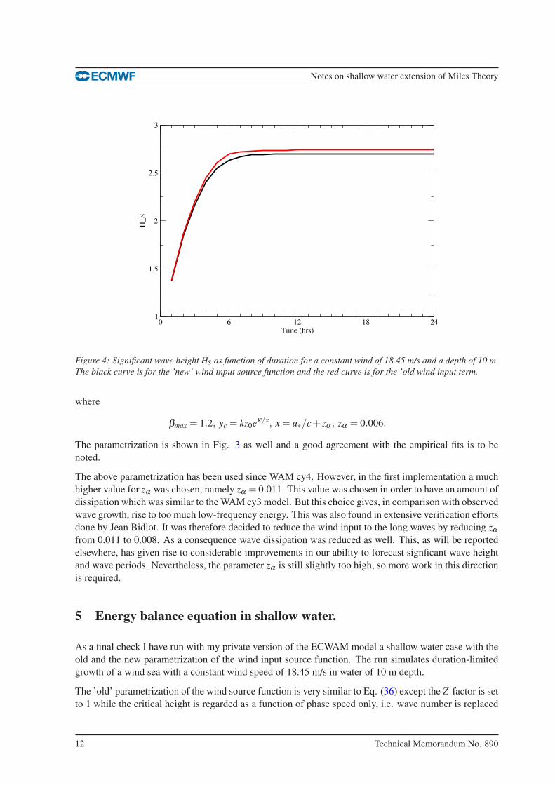
Figure 4: Significant wave height HS as function of duration for a constant wind of 18.45 m/s and a depth of 10 m.

The black curve is for the ’new’ wind input source function and the red curve is for the ’old wind input term.

where

βmax = 1.2, yc = kz0eκ/x, x = u∗/c+ zα , zα = 0.006.

The parametrization is shown in Fig. 3 as well and a good agreement with the empirical fits is to be

noted.

The above parametrization has been used since WAM cy4. However, in the first implementation a much

higher value for zα was chosen, namely zα = 0.011. This value was chosen in order to have an amount of

dissipation which was similar to the WAM cy3 model. But this choice gives, in comparison with observed

wave growth, rise to too much low-frequency energy. This was also found in extensive verification efforts

done by Jean Bidlot. It was therefore decided to reduce the wind input to the long waves by reducing zα

from 0.011 to 0.008. As a consequence wave dissipation was reduced as well. This, as will be reported

elsewhere, has given rise to considerable improvements in our ability to forecast signficant wave height

and wave periods. Nevertheless, the parameter zα is still slightly too high, so more work in this direction

is required.

5 Energy balance equation in shallow water.

As a final check I have run with my private version of the ECWAM model a shallow water case with the

old and the new parametrization of the wind input source function. The run simulates duration-limited

growth of a wind sea with a constant wind speed of 18.45 m/s in water of 10 m depth.

The ’old’ parametrization of the wind source function is very similar to Eq. (36) except the Z-factor is set

to 1 while the critical height is regarded as a function of phase speed only, i.e. wave number is replaced



0 0.5 1 1.5 2 2.5 3ω

0

0.2

0.4

0.6

0.8

1

1.2

1.4S

pec

tru

m F

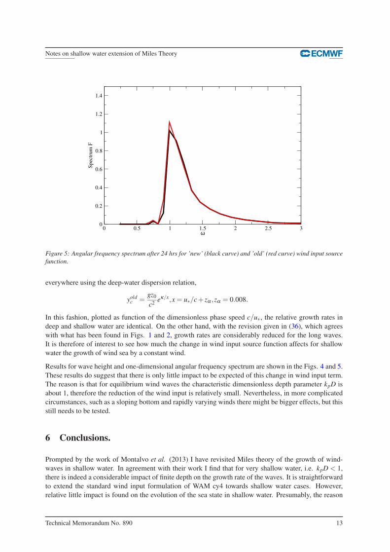
Figure 5: Angular frequency spectrum after 24 hrs for ’new’ (black curve) and ’old’ (red curve) wind input source

function.

everywhere using the deep-water dispersion relation,

yoldc =

gz0

c2eκ/x,x = u∗/c+ zα ,zα = 0.008.

In this fashion, plotted as function of the dimensionless phase speed c/u∗, the relative growth rates in

deep and shallow water are identical. On the other hand, with the revision given in (36), which agrees

with what has been found in Figs. 1 and 2, growth rates are considerably reduced for the long waves.

It is therefore of interest to see how much the change in wind input source function affects for shallow

water the growth of wind sea by a constant wind.

Results for wave height and one-dimensional angular frequency spectrum are shown in the Figs. 4 and 5.

These results do suggest that there is only little impact to be expected of this change in wind input term.

The reason is that for equilibrium wind waves the characteristic dimensionless depth parameter kpD is

about 1, therefore the reduction of the wind input is relatively small. Nevertheless, in more complicated

circumstances, such as a sloping bottom and rapidly varying winds there might be bigger effects, but this

still needs to be tested.

6 Conclusions.

Prompted by the work of Montalvo et al. (2013) I have revisited Miles theory of the growth of wind-

waves in shallow water. In agreement with their work I find that for very shallow water, i.e. kpD < 1,

there is indeed a considerable impact of finite depth on the growth rate of the waves. It is straightforward

to extend the standard wind input formulation of WAM cy4 towards shallow water cases. However,

relative little impact is found on the evolution of the sea state in shallow water. Presumably, the reason



for this is that in equilibrium the sea state in shallow water has a peak wavenumber kp that approximately

satisfies the condition kpD ≈ 1, in other words in practice shallow water effects on wind-wave growth

are relatively small.

Acknowledgement The author acknowledges useful and stimulating discussions with Miguel Onorato

and Jean Bidlot. He thanks Roger Grimshaw for confirming the mathematical results obtained in the

Appendix.



Appendix.

A Approximate solution of the Rayleigh Equation.

The following results have been obtained after a long-standing collaboration I had with Cees van Duijn in

the 1990’s. We usually worked in terms of the stream function Ψ defined in such a way that u=−∂Ψ/∂ z

and w = ∂Ψ/∂x. Therefore, the transition from the Fourier transform of the vertical velocity to the

Fourier transform of the stream function is straightforward since w = ikΨ. As in the main text the hats

will be dropped.

A.1 Statement of the problem.

Our starting point is the boundary value problem for the normalized vertical velocity χ given in Eq. (23)

with wind profile (24). The stream function Ψ is introduced through w = ikΨ, and the normalization by

w(0) is ignored. Next, we shift the origin of the vertical coordinate y by an amount y0 which results in

a simpler wind profile and the boundary condition at y = 0 is now applied at height y0. Thus, we search

for an approximate solution of the following boundary value problem:

W

(

d2

dy2−1

)

Ψ =W ′′Ψ,

Ψ(y0) =−c, (A1)

Ψ → 0, y → ∞.

where the prime now denotes differentiation of an equilibrium quantity with respect to y = k(z+ z0),with z is the distance from the water surface. Here, W =U0(y)− c with wind profile

U0 =u∗κ

log

(

y

y0

)

, (A2)

and the dimensionless roughness is given by y0 = kz0.

In order to make progress the following important relations are introduced. Define the scale velocity

V =U0(α), (A3)

where α will be determined in such a way that the convergence of the perturbation expansion is optimal.

Velocities will be scaled with V and we regard

ε =u∗V

=κ

log(α/y0)(A4)

as a small parameter. For a dimensionless phase speed c∗ = c/u∗ = 5 and a Charnock parameter αCH =0.0144 the small parameter ε ≈ 0.05. Another small parameter in the problem is y0. This parameter is

compared to ε exponentially small (for the example at hand one has y0 ≈ 0.0006), and therefore effects

of the order y0 will be ignored in the treatment that follows.

Scaled with V the wind profile becomes

U0 = 1+ε

κlog( y

α

)

. (A5)



Furthermore, the Doppler shifted velocity W =U0 − c may be written in a number of forms. With yc the

critical height and

c =U0(yc) = 1+ε

κlog(yc

α

)

. (A6)

one finds

W =ε

κlog

(

y

yc

)

. (A7)

This form is appropriate for the so-called inner region to be defined shortly. Introducing w = 1− c and

inverting Eq. (A6) the critical height can be written as

yc = αe−κwε , (A8)

and elimination of yc from (A7) gives an alternative form for W , namely

W = w+ε

κlog(

y

α). (A9)

This form will be used in the outer region.

Finally, we make a choice for the order of magnitude of the critical height yc. It is assumed that

yc = O(ε) (A10)

and therefore there are two regions/layers in this problem, an inner region of thickness O(ε), also called

the critical layer, and an outer region of thickness O(1).

Next, the relevant solutions in these two layers are discussed. These will be matched afterwards providing

an approximate solution to the problem (A1). In our expansion it will be assumed that y0 is much smaller

than ε and therefore effects of the order of y0 will be ignored.

A.2 Critical layer

In the critical layer we introduce the new variable ξ = y/ε , then the relevant differential equation be-

comes

(

Wd2

dξ 2−W ′′

)

Ψ = ε2WΨ (A11)

where W ′′ =−ε/(κξ 2) and W = εκ log(ξ/ξc). Note that ξc = yc/ε = O(1).

Therefore, in the critical layer W ′′ and W are of the same order of magnitude and the RHS is a small

correction. In order to obtain an approximate solution the Rayleigh equation is converted to an integral

equation. We pose

Ψ =WΦ

then

d

dξ

(

W 2 d

dξΦ

)

= ε2W 2Φ. (A12)



Integrating twice, using the boundary condition Ψ(y0) =−c, hence Φ(y0) = 1, one finds with ξ0 = y0/ε

Φ = 1+ εβ∫ ξ

ξ0

dη

W 2(η)+ ε2

∫ ξ

ξ0

dη

W 2(η)

∫ η

η0

dζ W 2(ζ )Φ(ζ ), (A13)

where from the outset we have chosen the second term to be of order ε . The constant β will be determined

by matching with the outer solution. In the present treatment we only need a solution up to first order in

ε . Thus,

Φ = 1+ εβK(ξ ), K(ξ ) =∫ ξ

ξ0

dη

W 2, (A14)

The integration contour in the integal defining the K-function is along the real axis, except near the

critical height where the contour is deformed by indentation below the real axis (assuming that U ′0c > 0).

In order to see this more clearly the integration variable is changed from η to W , hence

K(ξ ) =∫ W

W0

dW

W ′W 2,

where W0 =−c. The next step is to express W ′ in terms of W . With

W =ε

κlog(ξ/ξc)

one may express ξ in terms of W , i.e.

ξ = ξceκW

ε ,

and then

W ′ = ε/(κξ ) =W ′ce−

κWε .

As a consequence, with x = κW/ε and x0 = κW0/ε , the function K may therefore be written as

K(ξ ) =κ

εW ′c

∫ x

x0

dyey

y2.

Partial integration then gives

K(ξ ) =κ

εW ′c

(

− ey

y

∣

∣

∣

∣

x

x0

+∫ x

x0

dyey

y

)

. (A15)

The lower bound of the integral is in practice very large and negative. Therefore it may be replaced by

−∞. In that case the integral is connected to the Exponential Integral Ei defined as

Ei(x) =∫ x

−∞dy

ey

y= P

∫ x

−∞dy

ey

y+πiH(x),

with H(x) the Heaviside function. Thus, for x > 0, i.e. above the critical height, the K-function becomes

complex. There is therefore a phase jump above the critical height, a phenomenon that has been exten-

sively observed by Hristov et al. (2003). Thus, finally, the K-function becomes to good approximation

K(ξ ) =κ

εW ′c

(

−ex

x+Ei(x)

)

(A16)



For matching purposes we need the inner solution for large ξ , hence ξ >> ξc. With

P

∫ x

−∞dy

ey

y=

ex

x

(

1+1

x+

2

x2+ ...

)

one finds

limξ→∞

K(ξ ) =ξ

W 2

(

1+2ε

κW

)

+πi(κ

ε

)2

ξc.

Therefore, for large ξ the inner solution becomes

limξ→∞

Ψinner =W

[

1+ εβ

{

ξ

W 2

(

1+2ε

κW

)

+πi(κ

ε

)2

ξc

}]

.

In order to match to the solution in the outer region Ψinner is written in terms of the independent variable

y = εξ , while realizing that in the outer region the doppler shifted velocity is to first approximation a

constant, i.e. W = w+ εκ log(y/α). As a result one finds

Ψinner → w

(

1+βy

w2

)

+ε

κ

{

2βy

w2+ log

( y

α

)

(

1− βy

w2

)}

+

iβΓ[

w+ε

κlog( y

α

)]

(A17)

with

Γ = π(κ

ε

)2

yc.

A.3 Outer layer.

In the outer layer we assume a different balance by taking the curvature term to be small, so that now

(

Wd2

dy2−1

)

Ψ =W ′′Ψ = small. (A18)

In the outer layer we pose

Ψ = Φe−y,

then

d

dy

(

d

dyΦ−2Φ

)

= qΦ, q =W ′′

W,

hence, integrating once one has

d

dyΦ−2Φ =

∫ ∞

ydη q(η)Φ(η)+ const.

Another integration gives

Φ = F +1

2

∫ ∞

ydη(

1− e−2(η−y))

q(η)Φ(η).



In the outer layer y = O(1) and then q is found to be small as q(η) = −ε/(κwη2). The above integral

equation for Φ can then be solved by means of iteration and up to second order one finds

Φ = F +1

2F

∫ ∞

ydη(

1− e−2(η−y))

q(η).

Making use of the expression for q, the integral may be evaluated with the result

Ψouter = Fe−y(

1− ε

κwe2yE1(2y)

)

+ ....

which is identical to van Duin and Janssen (1992). Here E1 is another form of the exponential integral,

i.e.

E1(x) =∫ ∞

xdt

e−t

t.

The unknown F will be determined by matching with the inner solution, hence we have to evaluate Ψ

for small y. One finds

limy→0

Ψouter = F[

1− y+ε

κw

{

−2y+(1+ y) log( y

a

)}]

(A19)

with log(1/a) = γ + log2. Here we used E1(2y) = 2y− log(y/a) for y → 0.

A.4 Matching the critical layer and the outer layer.

We match now (A17) and (A19). In our approach we have introduced one additional degree of freedom

namely the height α of the scaling velocity V , see Eq. (A3), and this will be determined by higher order

matching.

Let us start with lowest order matching of the inner and outer solution. Hence, we only consider terms

that are of zeroth order in ε . Then

Ψ(0)outer = F (1− y) ,and Ψ0

inner = w

(

1+βy

w2+ iβΓ

)

Matching the constant terms then gives

F = w(1+ iβΓ)

while matching the y-terms gives

β =−wF

Eliminating β from the above two equations then results in

F =w

1+ iΓ, (A20)

while

β =− w2

1+ iΓ, (A21)



with Γ = w2Γ = π(κw/ε)2yc.

Let us now continue with first-order matching. In first order the outer solution gives the terms

Ψ(1)outer =

F

κw{−2y+(1+ y)(logy− loga)}

while the first-order inner solution reads

Ψ(1)inner =

F

κw{−2y+(1+ y)(logy− logα)} .

First of all, note that the (1+ y) logy terms match unconditionally. The y−terms match provided the

following condition on a is satisfied:

α = a =1

2e−γ

As a result we obtain a solution which is correct to first order in ε .

A.5 Growth rate.

The growth rate γE of the energy E of the gravity waves is connected to the pressure perturbation p at

the surface. From van Duin and Janssen (1992) one finds

γE

ω=

s

c2ℑ(p)

where the pressure perturbation in the critical layer follows from

p =1

ε

{

WdΨ

dξ−Ψ

dW

dξ

}

Using Ψ =WΦ then

p =1

εW 2 dΦ

dξ

Therefore, with (A14), one simply obtains

p = β =− w2

1+ iΓ.

As a consequence, the growth rate becomes

γE

ω=

s

c2ℑ(p) = s

(w

c

)2 Γ

1+ Γ2

Recall that Γ = w2Γ = π(κw/ε)2yc. Here, velocities have been scaled with V . In terms of friction

velocity scaling one finds for the growth rate

γE

ω= sβM

(u∗c

)2

(A22)

where

βM =(w

ε

)2 Γ

1+ Γ2



0 5 10 15 20 25 30c/u_*

0.01

0.1

1 epsilon

k z_c

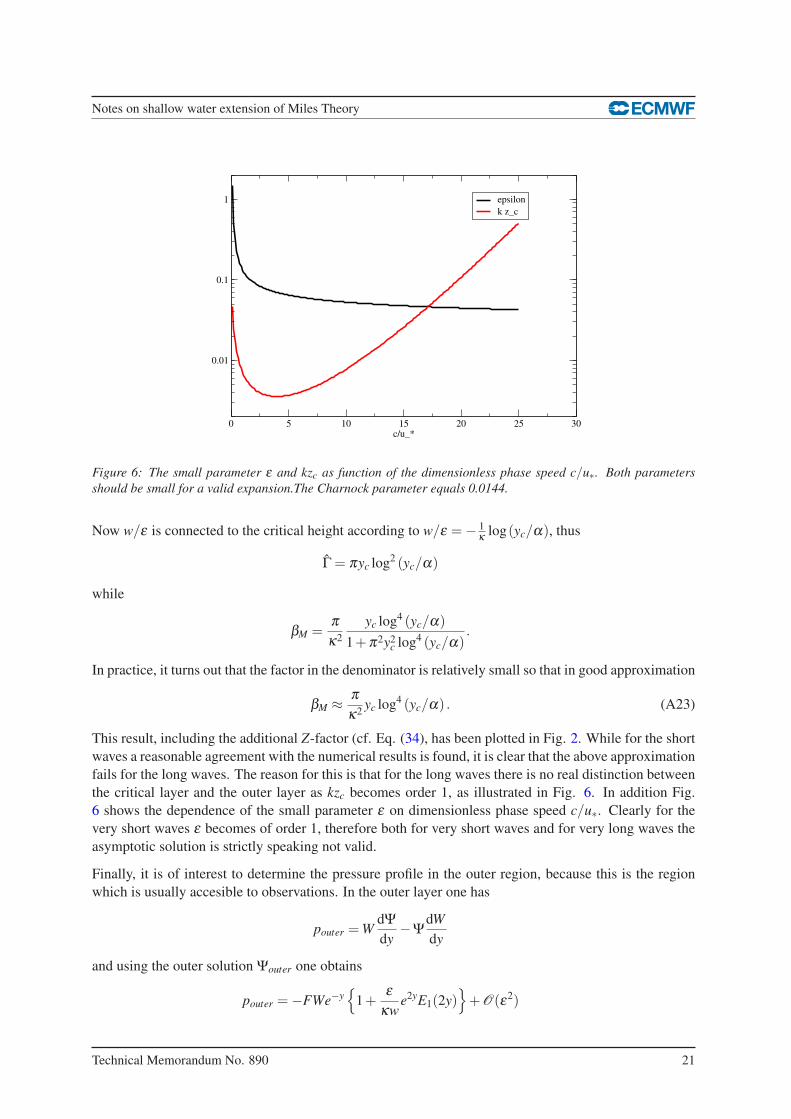
Figure 6: The small parameter ε and kzc as function of the dimensionless phase speed c/u∗. Both parameters

should be small for a valid expansion.The Charnock parameter equals 0.0144.

Now w/ε is connected to the critical height according to w/ε =− 1κ log(yc/α), thus

Γ = πyc log2 (yc/α)

while

βM =π

κ2

yc log4 (yc/α)

1+π2y2c log4 (yc/α)

.

In practice, it turns out that the factor in the denominator is relatively small so that in good approximation

βM ≈ π

κ2yc log4 (yc/α) . (A23)

This result, including the additional Z-factor (cf. Eq. (34), has been plotted in Fig. 2. While for the short

waves a reasonable agreement with the numerical results is found, it is clear that the above approximation

fails for the long waves. The reason for this is that for the long waves there is no real distinction between

the critical layer and the outer layer as kzc becomes order 1, as illustrated in Fig. 6. In addition Fig.

6 shows the dependence of the small parameter ε on dimensionless phase speed c/u∗. Clearly for the

very short waves ε becomes of order 1, therefore both for very short waves and for very long waves the

asymptotic solution is strictly speaking not valid.

Finally, it is of interest to determine the pressure profile in the outer region, because this is the region

which is usually accesible to observations. In the outer layer one has

pouter =WdΨ

dy−Ψ

dW

dy

and using the outer solution Ψouter one obtains

pouter =−FWe−y{

1+ε

κwe2yE1(2y)

}

+O(ε2)



where W = w+ εκ log(y/α) and F = w/(1+ iΓ). In order to check that we have followed a proper

matching procedure one would expect that the pressure is continuous and that the limit of small height

of the outer pressure should be equal to the critical layer pressure. This is indeed the case as

pouter =−FWe−y +O(ε) =− w2

1+ iΓ

which agrees with the critical layer pressure result p = β .

References

Conte, S.D. and J.W. Miles, 1959. On the integration of the Orr-Sommerfeld equation. J. Soc. Indust.

Appl. Math. 7, 361-369.

Duin, C.A. van and P.A.E.M. Janssen, 1992. An analytic model of the generation of surface gravity

waves by turbulent air flow. J. Fluid Mech. 236, 197-215.

Hristov, T.S., S.D. Miller and C.A. Friehe, 2003: Dynamical coupling of wind and ocean waves through

wave-induced air flow. Nature, 442, 55-58.

Janssen, P., 2004 The Interaction of Ocean Waves and Wind, Cambridge University Press, Cambridge,

U.K., 300+viii pp.

Miles, J.W., 1957. On the generation of surface waves by shear flows. J. Fluid Mech. 3, 185-204.

Miles, J.W., 1993. Surface wave generation revisited. J. Fluid Mech. 256, 427-441.

Montalvo, P., Dorignac, J., Manna M.A., Kharif C. and H. Branger, 2013. Growth of surface wind-waves

in water of finite depth. A theoretical approach. Coastal Engineering 77, 49-56.

Plant, W.J., 1982. A relation between wind stress and wave slope. J. Geophys. Res. C87, 1961-1967.

Snyder, R.L., F.W. Dobson, J.A. Elliott and R.B. Long, 1981. Array measurements of atmospheric

pressure fluctuations above surface gravity waves. J. Fluid Mech. 102, 1-59.


Documents

Technical Memo - ECMWF