Embed Size (px)
Citation preview
ECMWF Newsletter No. 102 – Winter 2004/05
1
Editorial
On page 2 Thierry Lefort (Météo-France) out-lines the progress that forecasters have madein medium-range forecasting for New Cale-
donia using ECMWF and other forecast products,while on page 7 François Lalaurette gives an update onrecent developments at ECMWF in predicting tropi-cal cyclones in the early medium-range, and describessome new products available on the web site.The dif-ficult practical decisions that forecasters have to makewhen faced with the threat of severe weather are dis-cussed on page 15 by members of the Turkish WeatherService.The article on page 16 by Martin Leutbecherand colleagues describes some experiments to assessthe usefulness of making additional targeted observa-tions in areas that are considered likely to be sensitivefor the subsequent forecast. Details of the improve-ments made to the Integrated Forecasting System intwo recent cycles – Cycle 26r3 (operational on 7October 2003) and Cycle 28r1 (operational on 9March 2004) – are given by Jean-Noël Thépaut andcolleagues on page 26. Finally, on page 36 JohnHennessy looks back into the early history of theCentre and describes the problems involved in pro-ducing the first operational forecasts 25 years ago.
Peter WhiteEuropean Centre forMedium-Range Weather Forecasts
Shinfield Park, Reading, Berkshire RG2 9AX, UK
Fax: . . . . . . . . . . . . . . . . . . . . . . . .+44 118 986 9450
Telephone: National . . . . . . . . . . . . .0118 949 9000
International . . . . . . .+44 118 949 9000
ECMWF Web site . . . . . . . . . .http://www.ecmwf.int
The ECMWF Newsletter is published quarterly andcontains articles about new developments and systemsat ECMWF. Articles about uses and applications ofECMWF forecasts are also welcome from authorsworking elsewhere (especially those from MemberStates and Co-operating States).
The ECMWF Newsletter is not a peer-reviewedpublication.
Editor: Peter White
Typesetting and Graphics: Rob Hine
Front Cover
New Caledonia and (inset) Tropical Cyclone Erica:– see articles onpages 2 and 7. © Thierry Lefort.
In this issue
Editorial . . . . . . . . . . . . . . . . . . . . . . . . . . . . . . . . . 1
Changes to the operational weather prediction system 1
METEOROLOGY
Starting up medium-range forecasting for NewCaledonia in the South-West Pacific Ocean –a not so boring tropical climate. . . . . . . . . . . . . . . . . 2
Early medium-range forecasts of tropical cyclones . . . 7
A snowstorm in north-western Turkey12–13 February 2004 –Forecasts, public warnings and lessons learned – . . . . 15
Planning of adaptive observations during theAtlantic THORPEX Regional Campaign 2003 . . . . 16
Two new cycles of the IFS: 26r3 and 28r1 . . . . . . . . 26
COMPUTING
25 years since the first operational forecast . . . . . . . . 36
GENERAL
61st Council session on 13–14 December 2004 . . . . 39
ECMWF Calendar 2005. . . . . . . . . . . . . . . . . . . . . 40
MARS reaches one Petabyte . . . . . . . . . . . . . . . . . . 40
ECMWF publications. . . . . . . . . . . . . . . . . . . . . . . 40
New items on the ECMWF web site . . . . . . . . . . . 41
Index of past newsletter articles . . . . . . . . . . . . . . . . 42
Useful names and telephone numberswithin ECMWF. . . . . . . . . . . . . . . . . . . . . . . . . . . 44
Changes to the operationalweather prediction system
28 September 2004 – Cycle 28r3 was introduced. Thisincluded changes to the:u Physics – Revised numerics of the convection scheme
and the calling of the cloud scheme; use of the tangentlinear and adjoint of vertical diffusion in the first mini-mization of 4D-Var; reduction of the radiation frequencyto one hour in the high-resolution forecasts; improvednumerics of surface tile coupling; post-processing oftotal-column liquid water and ice.
u Use of satellite data – RTTOV-8; minor revisions toATOVS and AIRS usage; assimilation of MSG clear-skyradiances and GOES-9 BUFR AMVs; assimilation ofSCIAMACHY ozone products from KNMI; correctionof error in AMSU-B usage over land; activation of EARSdata.
u Data assimilation – Blacklist SYNOP humidity data atlocal night time; increased use of radiosonde humidity(using RS90 to -80°C, RS80 to -60°C, other sensors to-40°C); proper cycling of the information from the wavealtimeter and the surface data analyses (first-guess fore-casts moved from 00 and 12 UTC to 06 and 18 UTC).

ECMWF Newsletter No. 102 – Winter 2004/05METEOROLOGY
2
New Caledonia is located 1500km east of Queens-land,Australia, between 18°S and 23°S. Its surfaceis 19,000km2.The main island or Grande Terre is
400km long and 50km wide,with a mountain range roughlyparallel to the coasts that reaches 1000 to 1600m in altitude.Smaller islands are located to the north and to the south.Thelagoon is 8000km2 in area and as much as 65km wide. Onehundred kilometres to the east lie the Loyauté islands; theseare flat, coral islands (Figure 1).
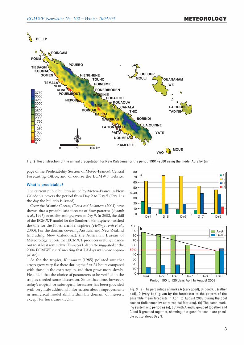
New Caledonia is located just north of the Tropic ofCapricorn,but its climate is said to be ‘maritime tropical’.Theyear is divided roughly into two periods.The cool season lastsfrom May to October: extratropical lows form in the TasmanSea and we get occasional cold fronts associated with shortperiods of westerlies.The average low temperature in July is11.8°C in the western lowlands, so that morning tempera-tures of less than 10°C are frequent.The lowest temperaturerecorded in flat areas is 2.3°C on the Grande Terre, and 2.7°Con the Loyauté islands! The hot season lasts from Novemberto April; it is also called the tropical-cyclone or rainy season.Since the elongated Grande Terre is roughly perpendicular tothe prevailing easterlies, there is a considerable differencebetween the east coast,which is humid and green,and the westcoast, which is much drier in the lee of the range (Figure 2).
As New Caledonia is a French Territory, Météo-Franceis in charge of meteorology.The last decade has seen tremen-dous changes in the working environment of Météo-Franceforecasters in New Caledonia: the workstation Synergiewas installed in 1994; two precipitation radars are now oper-ating,with a third due to be operating soon; and the forecasteris provided with several global models, including the Frenchmodel ARPEGE TROPIQUE and the ECMWF T511 fieldsdisplayed on a 0.5 degree grid at six-hour intervals. Ensembleproducts are also available from the workstation, the Intranet
Starting up medium-range forecasting for New Caledonia inthe South-West Pacific Ocean – a not so boring tropical climate
0 50 100 km
KoumacPoindimie OUANAHAM
La Tontouta
40003000200010000 Noumea
New Caledonia
Fig. 1 (upper) A map of south-west Pacific Ocean. The oval showsthe New Caledonian territory. The square is the domain for tropicalcyclone warnings. The diamond-shape is the domain for marinebulletins. (lower) Detail of New Caledonia and the nearby islands.
u EPS – Gaussian sampling for extratropical singular vectorsinstead of selection and rotation; revision of initial-condi-tion perturbations for tropical cyclones (initial conditionperturbations extended to latitude belts 40°S and 40°Nfrom 25°S and 25°N, and tropical singular vectors arecomputed in the subspace orthogonal to the leading 25extratropical singular vectors); new algorithm to deter-mine optimisation regions based on predicted tropicalcyclone tracks from previous EPS run (the Caribbeanremains an optimisation region if no tropical cyclone is
in the vicinity); orthonormalisation applied to the set ofall tropical singular vectors ).
7 October 2004 – Monthly forecasts run operationally ona weekly basis (Thursdays).18 October 2004 – The bias correction for AMSU-A andAIRS satellites was harmonised. The bias correction forAMSU-B and HIRS was simplified to use two predictors.9 November 2004 – All four BC-project analyses used back-ground fields generated from the latest operational 4D-Varanalysis
François Lalaurette
Phot
ogra
ph ©
Thi
erry
Lef
ort
ECMWF Newsletter No. 102 – Winter 2004/05
3
METEOROLOGY
page of the Predictability Section of Météo-France’s CentralForecasting Office, and of course the ECMWF website.
What is predictable?
The current public bulletin issued by Météo-France in NewCaledonia covers the period from Day 2 to Day 5 (Day 1 isthe day the bulletin is issued).
Over the Atlantic Ocean, Chessa and Lalaurette (2001) haveshown that a probabilistic forecast of flow patterns (Ayraultet al., 1995) beats climatology, even at Day 9. In 2002, the skillof the ECMWF model for the Southern Hemisphere matchedthe one for the Northern Hemisphere (Hollingsworth et al.,2003). For the domain covering Australia and New Zealand(including New Caledonia), the Australian Bureau ofMeteorology reports that ECMWF produces useful guidanceout to at least seven days (François Lalaurette suggested at the2004 ECMWF users’meeting that 71⁄2 days was more appro-priate).
As for the tropics, Kanamitsu (1985) pointed out thaterrors grow very fast there during the first 24 hours comparedwith those in the extratropics, and then grow more slowly.He added that the choice of parameters to be verified in thetropics needed some discussion. Since that time, however,today’s tropical or subtropical forecaster has been providedwith very little additional information about improvementsin numerical model skill within his domain of interest,except for hurricane tracks.
AOUPINIE
BELEP
BORINDI
CANALA
HIENGHENE
HOUAILOU
KOUAOUA
MOUE
MOULI OUANAHAM
OULOUP
POINDIMIE
POINGAM
PONERIHOUEN
POUEBO
TOUHO
WE
YATE
LA OUINNE
THIOBOURAIL
GOMEN
KONE
KOUMAC
LA FOA
LA TONTOUTA
NOUMEA
PAITA
P.AMEDEE
POUM
TIEBAGHI
POUEMBOUT
TEMALA
VAO
NEPOUI
VOH
LA ROCHE
TADINE
NASSIRAH
MEA
0500750100012501500175020002250250027503000325035003750
0 50 100 km
Fig. 2 Reconstruction of the annual precipitation for New Caledonia for the period 1991–2000 using the model Aurelhy (mm).
0
10
20
30
40
50
60
70
%
80
D+4 D+5 D+6 D+7 D+9
ABCD
10090807060
50%
40302010
0
A+BC+D
Period: 100 to 120 days April to August 2003D+4 D+5 D+6 D+7 D+8 D+9
Fig. 3 (a) The percentage of marks A (very good), B (good), C (ratherbad), D (very bad) given by the forecaster to the pattern of theensemble mean forecasts in April to August 2003 during the coolseason (influenced by extratropical features). (b) The same mark-ing system and period as (a), but with A and B grouped together andC and D grouped together, showing that good forecasts are possi-ble out to about Day 9.
a
b
ECMWF Newsletter No. 102 – Winter 2004/05METEOROLOGY
4
The Ensemble Prediction System (EPS) provides a usefulguidance for the New Caledonian forecaster up to Day 8
We decided to start a subjective evaluation of the EPS for NewCaledonia.We used standard charts available at the time: theensemble means of the 1000 hPa geopotential (Z1000), the850 hPa temperature (T850) and the 500 hPa geopotentialand temperature (ZT500), as well as the precipitation onthreshold probability maps over the south-west Pacific domain.Marks were given by one forecaster for the accuracy of fore-casts from 108 hours (noon local time on Day 5) to 228 hours(noon on Day 10) according to the following:A Large-scale and details correct;B Large-scale correct, but some details wrong;C Large-scale correct but the flow pattern too wrong
around New Caledonia to allow a good forecast;D Large-scale totally wrong.
The results for a four-month period (mostly during thecool season) are presented in Figures 3(a) and (b). Up to Day8, the ensemble mean seems to allow the forecaster to predictthe type of circulation induced by the movements of thesubtropical anticyclones, the position of the intertropicalconvergence zone (ITCZ), etc.
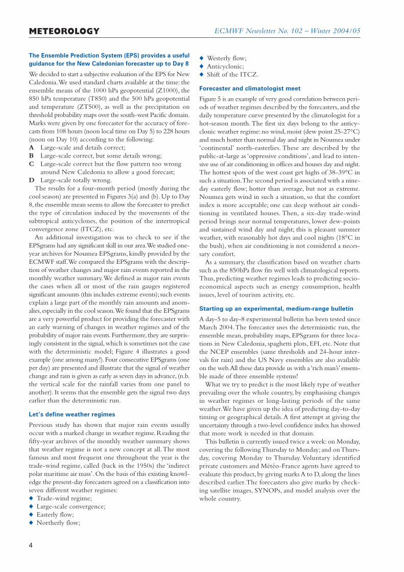
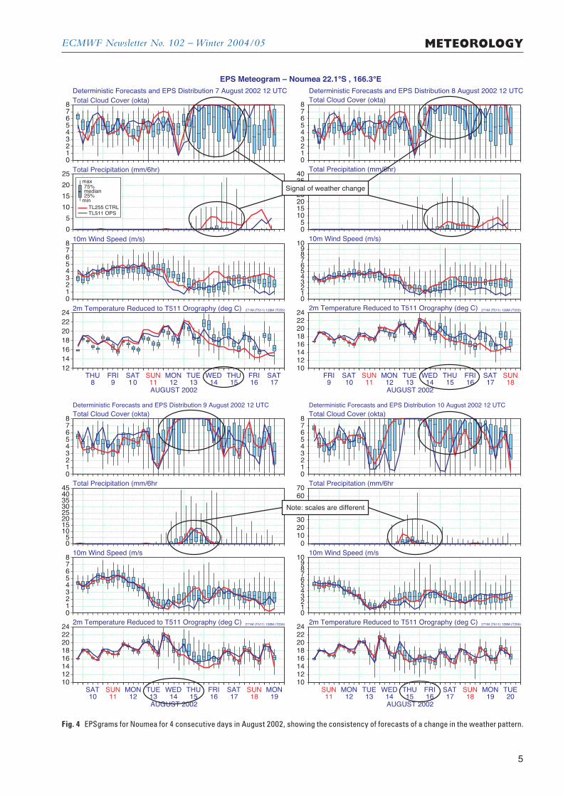
An additional investigation was to check to see if theEPSgrams had any significant skill in our area.We studied one-year archives for Noumea EPSgrams, kindly provided by theECMWF staff.We compared the EPSgrams with the descrip-tion of weather changes and major rain events reported in themonthly weather summary.We defined as major rain eventsthe cases when all or most of the rain gauges registeredsignificant amounts (this includes extreme events); such eventsexplain a large part of the monthly rain amounts and anom-alies, especially in the cool season.We found that the EPSgramsare a very powerful product for providing the forecaster withan early warning of changes in weather regimes and of theprobability of major rain events.Furthermore, they are surpris-ingly consistent in the signal,which is sometimes not the casewith the deterministic model; Figure 4 illustrates a goodexample (one among many!).Four consecutive EPSgrams (oneper day) are presented and illustrate that the signal of weatherchange and rain is given as early as seven days in advance, (n.b.the vertical scale for the rainfall varies from one panel toanother). It seems that the ensemble gets the signal two daysearlier than the deterministic run.
Let’s define weather regimes
Previous study has shown that major rain events usuallyoccur with a marked change in weather regime.Reading thefifty-year archives of the monthly weather summary showsthat weather regime is not a new concept at all.The mostfamous and most frequent one throughout the year is thetrade-wind regime, called (back in the 1950s) the ‘indirectpolar maritime air mass’. On the basis of this existing knowl-edge the present-day forecasters agreed on a classification intoseven different weather regimes:u Trade-wind regime;u Large-scale convergence;u Easterly flow;u Northerly flow;
u Westerly flow;u Anticyclonic;u Shift of the ITCZ.
Forecaster and climatologist meet
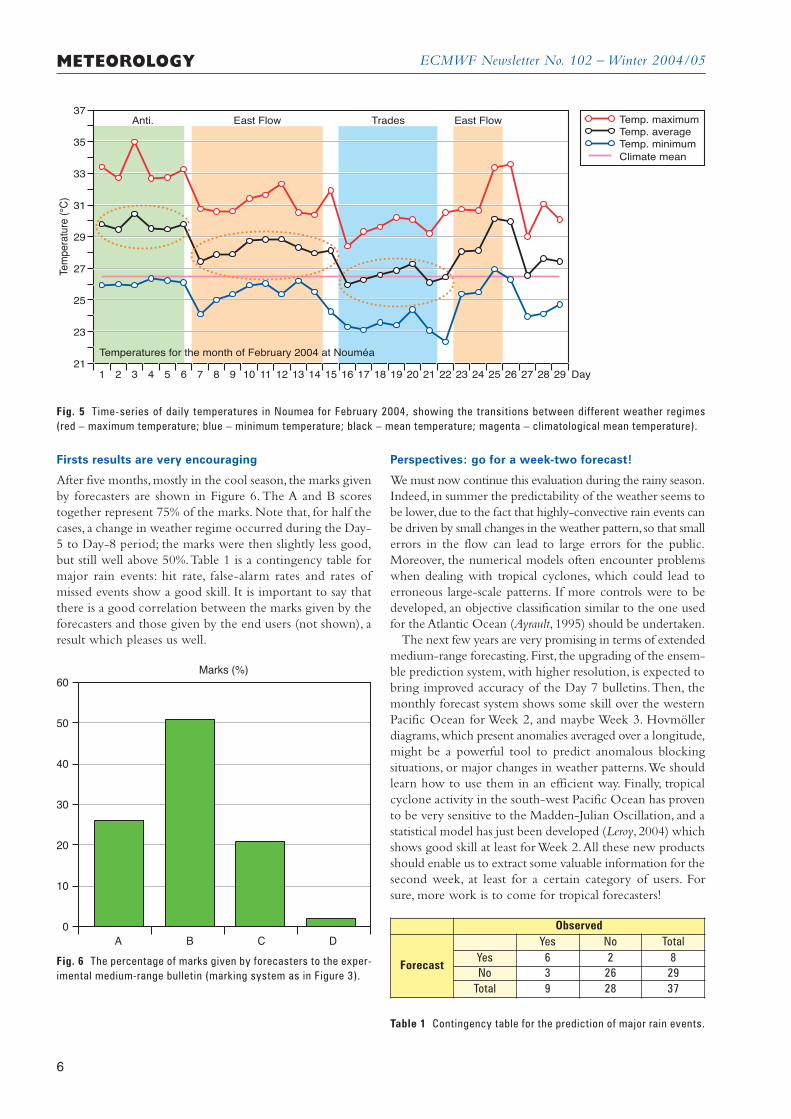
Figure 5 is an example of very good correlation between peri-ods of weather regimes described by the forecasters, and thedaily temperature curve presented by the climatologist for ahot-season month.The first six days belong to the anticy-clonic weather regime: no wind,moist (dew point 25-27°C)and much hotter than normal day and night in Noumea under‘continental’ north-easterlies. These are described by thepublic-at-large as ‘oppressive conditions’, and lead to inten-sive use of air conditioning in offices and houses day and night.The hottest spots of the west coast get highs of 38-39°C insuch a situation.The second period is associated with a nine-day easterly flow; hotter than average, but not as extreme.Noumea gets wind in such a situation, so that the comfortindex is more acceptable; one can sleep without air condi-tioning in ventilated houses. Then, a six-day trade-windperiod brings near normal temperatures, lower dew-pointsand sustained wind day and night; this is pleasant summerweather, with reasonably hot days and cool nights (18°C inthe bush), when air conditioning is not considered a neces-sary comfort.
As a summary, the classification based on weather chartssuch as the 850hPa flow fits well with climatological reports.Thus, predicting weather regimes leads to predicting socio-economical aspects such as energy consumption, healthissues, level of tourism activity, etc.
Starting up an experimental, medium-range bulletin
A day-5 to day-8 experimental bulletin has been tested sinceMarch 2004.The forecaster uses the deterministic run, theensemble mean, probability maps, EPSgrams for three loca-tions in New Caledonia, spaghetti plots, EFI, etc. Note thatthe NCEP ensembles (same thresholds and 24-hour inter-vals for rain) and the US Navy ensembles are also availableon the web.All these data provide us with a ‘rich man’s’ ensem-ble made of three ensemble systems!
What we try to predict is the most likely type of weatherprevailing over the whole country, by emphasising changesin weather regimes or long-lasting periods of the sameweather.We have given up the idea of predicting day-to-daytiming or geographical details.A first attempt at giving theuncertainty through a two-level confidence index has showedthat more work is needed in that domain.
This bulletin is currently issued twice a week: on Monday,covering the following Thursday to Monday; and on Thurs-day, covering Monday to Thursday. Voluntary identifiedprivate customers and Météo-France agents have agreed toevaluate this product, by giving marks A to D, along the linesdescribed earlier.The forecasters also give marks by check-ing satellite images, SYNOPs, and model analysis over thewhole country.
ECMWF Newsletter No. 102 – Winter 2004/05
5
METEOROLOGY
Fig. 4 EPSgrams for Noumea for 4 consecutive days in August 2002, showing the consistency of forecasts of a change in the weather pattern.
THU FRI SAT SUN MON TUE WED THU FRI SAT8
AUGUST 20029 10 11 12 13 14 15 16 17
Deterministic Forecasts and EPS Distribution 7 August 2002 12 UTC
EPS Meteogram – Noumea 22.1°S , 166.3°E
12141618202224
2m Temperature Reduced to T511 Orography (deg C) 271M (T511) 128M (T255)
012345678
10m Wind Speed (m/s)0
5
10
15
20
25Total Precipitation (mm/6hr)
012345678
Total Cloud Cover (okta)
max
min25%
75%median
TL255 CTRLTL511 OPS
FRI SAT SUN MON TUE WED THU FRI SAT SUN9
AUGUST 200210 11 12 13 14 15 16 17 18
Deterministic Forecasts and EPS Distribution 8 August 2002 12 UTC
1012141618202224
2m Temperature Reduced to T511 Orography (deg C) 271M (T511) 128M (T255)
0123456789
1010m Wind Speed (m/s)
05
10152025303540
Total Precipitation (mm/6hr)012345678
Total Cloud Cover (okta)
SAT SUN MON TUE WED THU FRI SAT SUN MON10
AUGUST 200211 12 13 14 15 16 17 18 19
Deterministic Forecasts and EPS Distribution 9 August 2002 12 UTC
1012141618202224
2m Temperature Reduced to T511 Orography (deg C) 271M (T511) 128M (T255)
012345678
10m Wind Speed (m/s05
1015202530354045
Total Precipitation (mm/6hr012345678
Total Cloud Cover (okta)
SUN MON TUE WED THU FRI SAT SUN MON TUE11
AUGUST 200212 13 14 15 16 17 18 19 20
Deterministic Forecasts and EPS Distribution 10 August 2002 12 UTC
1012141618202224
2m Temperature Reduced to T511 Orography (deg C) 271M (T511) 128M (T255)
0123456789
1010m Wind Speed (m/s
010203040506070
Total Precipitation (mm/6hr012345678
Total Cloud Cover (okta)
Signal of weather change
Note: scales are different
Marks (%)
0
10
20
30
40
50
60
A B C D
ECMWF Newsletter No. 102 – Winter 2004/05METEOROLOGY
6
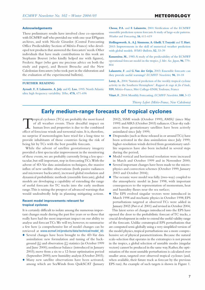
Firsts results are very encouraging
After five months,mostly in the cool season, the marks givenby forecasters are shown in Figure 6. The A and B scorestogether represent 75% of the marks. Note that, for half thecases, a change in weather regime occurred during the Day-5 to Day-8 period; the marks were then slightly less good,but still well above 50%.Table 1 is a contingency table formajor rain events: hit rate, false-alarm rates and rates ofmissed events show a good skill. It is important to say thatthere is a good correlation between the marks given by theforecasters and those given by the end users (not shown), aresult which pleases us well.
Perspectives: go for a week-two forecast!
We must now continue this evaluation during the rainy season.Indeed, in summer the predictability of the weather seems tobe lower,due to the fact that highly-convective rain events canbe driven by small changes in the weather pattern, so that smallerrors in the flow can lead to large errors for the public.Moreover, the numerical models often encounter problemswhen dealing with tropical cyclones, which could lead toerroneous large-scale patterns. If more controls were to bedeveloped, an objective classification similar to the one usedfor the Atlantic Ocean (Ayrault, 1995) should be undertaken.
The next few years are very promising in terms of extendedmedium-range forecasting.First, the upgrading of the ensem-ble prediction system, with higher resolution, is expected tobring improved accuracy of the Day 7 bulletins.Then, themonthly forecast system shows some skill over the westernPacific Ocean for Week 2, and maybe Week 3. Hovmöllerdiagrams,which present anomalies averaged over a longitude,might be a powerful tool to predict anomalous blockingsituations, or major changes in weather patterns.We shouldlearn how to use them in an efficient way. Finally, tropicalcyclone activity in the south-west Pacific Ocean has provento be very sensitive to the Madden-Julian Oscillation, and astatistical model has just been developed (Leroy, 2004) whichshows good skill at least for Week 2.All these new productsshould enable us to extract some valuable information for thesecond week, at least for a certain category of users. Forsure, more work is to come for tropical forecasters!
Fig. 6 The percentage of marks given by forecasters to the exper-imental medium-range bulletin (marking system as in Figure 3).
Observed
Forecast
Yes No TotalYes 6 2 8No 3 26 29
Total 9 28 37
Table 1 Contingency table for the prediction of major rain events.
Anti. East Flow East FlowTrades
1 2
35
37
33
31
29
27
25
23
213 4 5 6 7 8 9 10 11 12 13 14 15 16 17 18 19 20 21 22 23 24 25 26 27 28 29 Day
Tem
pera
ture
(°C
)
Temp. maximumTemp. averageTemp. minimumClimate mean
Temperatures for the month of February 2004 at Nouméa
Fig. 5 Time-series of daily temperatures in Noumea for February 2004, showing the transitions between different weather regimes(red – maximum temperature; blue – minimum temperature; black – mean temperature; magenta – climatological mean temperature).
ECMWF Newsletter No. 102 – Winter 2004/05 METEOROLOGY
7
Acknowledgements
These preliminary results have involved close co-operationwith ECMWF staff who provided me with one-year EPSgramarchives, and with Nicole Girardot (Central ForecastingOffice Predictability Section of Météo-France) who devel-oped test products that answered the forecasters’ needs.Otherindividuals that have made contributions to this work areStephanie Bouvet (who kindly helped me with figures),Frederic Atger (who gave me precious advice on both thestudy and paper), and Benoit Broucke and the NewCaledonian forecasters (who took part in the elaboration andthe evaluation of the experimental bulletin).
FURTHER READING
Ayrault, F., F. Lalaurette, A. Joly and C. Loo, 1995: North Atlanticultra high frequency variability. Tellus, 47A, 671-696
Chessa, P.A. and F. Lalaurette, 2001:Verification of the ECMWFensemble prediction system forecasts:A study of large-scale patterns.Weather and Forecasting, 16, 611-619
Hollingsworth, A., A.J. Simmons, A. Ghelli, T.Tsuyuki and T. Hart;2003: Improvements in the skill of numerical weather predictionwith global models. WMO Bulletin, 52, 33-39
Kanamitsu, M., 1985:A study of the predictability of the ECMWFoperational forecast model in the tropics. J. Met. Soc. Japan, 96, 779-804
Lalaurette, F. and G.Van der Grijn, 2003: Ensemble forecasts: canthey provide useful warnings? ECMWF Newsletter, 96, 10-18
Leroy, A., 2004:‘Statistical prediction of the weekly tropical cycloneactivity in the Southern Hemisphere’. Rapport de stage de fin d’étude,939, Météo-France, Met College-ENM,Toulouse, France
Vitart,F., 2004: Monthly Forecasting. ECMWF Newsletter,100, 3-13
Thierry Lefort (Météo-France, New Caledonia)
Early medium-range forecasts of tropical cyclones
Tropical cyclones (TCs) are probably the most fearedof all weather events. Their dreadful impact onhuman lives and properties is due to the combined
effect of ferocious winds and torrential rains. It is, therefore,no surprise if meteorologists have tried for a long time toprovide inhabitants of those countries facing the risk ofbeing hit by TCs with the best possible forecasts.
While the advent of satellite geostationary imageryprovided a first spectacular improvement in the monitoringof these events, we are probably currently living a less spec-tacular, but still important, step in forecasting TCs.With theadvent of 4D-Var data assimilation techniques, the massiveinflux of new satellite observations (both passive radiancesand microwave backscatter), increased global resolution anddynamical probabilistic methods (ensemble forecasts), globalmodels are developing a capability of extending the rangeof useful forecasts for TC tracks into the early mediumrange.This is raising the prospect of advanced warnings thatwould undoubtedly help in planning mitigating actions.
Recent model improvements relevant fortropical cyclones
It is certainly difficult to isolate among the numerous impor-tant changes made during the past five years or so those thatreally have had the most important impact on our ability toanalyse and forecast TCs.We will try, however, to summarisea few here (a comprehensive list of model changes can beretrieved at www.ecmwf.int/products/data/technical/model_id):u Several changes have been brought to the 4D-Var data
assimilation: new formulation and tuning of the back-ground (Jb) and observation (Jo) statistics (in October 1999and June 2000); nonlinear balance (introduced in January2003); move from a six to a 12-hour optimisation period(September 2000); new humidity analysis (October 2003);
u Many new satellite observations have been activated,among which are SeaWinds from QuikSCAT (January
2002), SSMI winds (October 1999), AMSU (since May1999) and AIRS (October 2003) radiances.Clear-sky radi-ances from geostationary satellites have been activelyassimilated since July 1999;
u Dropsondes (such as those released in or around TCs) havebeen activated in the data assimilation since July 1999;higher-resolution winds derived from geostationary satel-lite sequences have also been included in several stepsduring the period;
u Model vertical and horizontal resolution were increasedin March and October 1999 and in November 2000;
u Several important changes have been made to the micro-physics and convection schemes (October 1999, January2003 and October 2004);
u The oceanic wave model was fully (two-way) coupled tothe atmospheric model in June 1998, with importantconsequences to the representation of momentum, heatand humidity fluxes near the sea surface;
u The EPS evolved singular vectors were introduced inMarch 1998 and stochastic physics in October 1998; EPSperturbations targeted at observed TCs were added inJanuary 2002 (Puri et al. 2001) and revised in October 2004;
This latest series of changes introduced into the EPS haveopened the door to the probabilistic forecast of TC tracks, acrucial development in order to extend the useful validity rangeof the forecasts. Unlike extratropical EPS perturbations thatare computed semi-globally using a very simplified version ofthe model physics, tropical perturbations use a more compre-hensive set of physical parametrizations. Because the naturalscale-selection that operates in the extratropics is not presentin the tropics, a global selection of unstable modes (singularvectors) cannot be produced in the same way.Rather, the opti-misation of the most unstable perturbations is calculated oversmaller areas, targeted over observed tropical cyclones (and,when available, their future track as forecast by the previousEPS run).An example of such targets is shown in Figure 1.
ECMWF Newsletter No. 102 – Winter 2004/05METEOROLOGY
8
To keep a fair balance, it should be remembered that thereare still severe limitations in the model’s ability to copewith TCs.u Insufficient resolution is obviously one limitation. In no
way can the eye of the cyclone (where surface pressuredrops to very low values over a short distance) be resolvedwith an 80 km, or even a 40 km, resolution model.Thesituation is even worse in terms of the analysis (incrementscurrently have only about a 130 km resolution);
u The non-interaction between the atmospheric and oceaniccomponents is another limitation. Indeed the sea surfacetemperatures (SSTs) are kept constant during the modelintegration (only the monthly and seasonal forecast modelscurrently have an interactive ocean).
Both of these have important consequences in terms ofthe ability of our system to predict the intensity of the TCscorrectly. Rather than providing a realistic description of thepowerful energy cycle that occurs within a TC (for theupper layers of the ocean this is an important component),the model currently only represents a crude approximationof an axisymmetric circulation whose intensity is stronglyunderestimated compared with most energetic TCs. As isshown later in this article, there is undoubtedly skill in themodel forecasts of TC tracks-much more so than ten, or evenfive, years ago. It is to get an objective evaluation of such askill that a TC tracker has been developed at ECMWF inrecent years, and recently (October 2004) turned into anoperational application.
Tracking the cyclone
It is important to stress that the tracker described here is apure diagnostic of the model’s ability to detect (analyse)
and forecast the displacement, growth and decay of TCs. Itdoes not interfere with the model’s dynamics.The trackingalgorithm simply tries to detect, in the area where the TChas been reported, features in the model fields (pressure,vorticity, temperature) that are characteristic of TCs. If thesefeatures are detected, the tracker then tries to follow thesystem in subsequent forecast steps-for the deterministicmodel as well as for all EPS members.The tracker finally storesinformation about cyclone position and intensity in theECMWF general-purpose meteorological archive facility(MARS). It can then be used for the generation of forecastproducts or for verification purposes.
Just like the targeting that is described above, the track-ing algorithm is fed with TC observation data.The ECMWFTC tracker will, therefore, only run for TCs for which thereis an observation available within the data assimilation timewindow (0300-1500 UTC for a 1200 UTC run, 1500-0300 UTC for a 0000 UTC run). It is important to stressthat, at this stage, no identification of TCs that may begenerated during the forecast is attempted.A first descrip-tion of the tracker has been published by van der Grijn(2002); an updated version following improvements suggestedby experience is given later in this article.
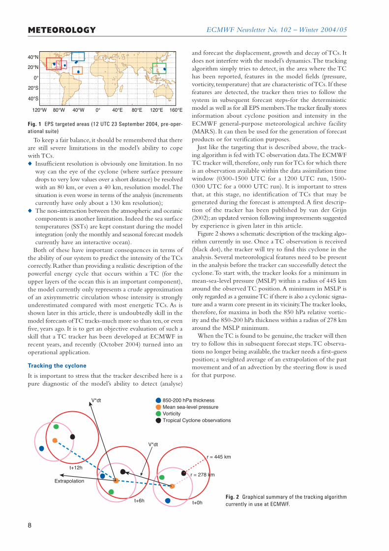
Figure 2 shows a schematic description of the tracking algo-rithm currently in use. Once a TC observation is received(black dot), the tracker will try to find this cyclone in theanalysis. Several meteorological features need to be presentin the analysis before the tracker can successfully detect thecyclone.To start with, the tracker looks for a minimum inmean-sea-level pressure (MSLP) within a radius of 445 kmaround the observed TC position.A minimum in MSLP isonly regarded as a genuine TC if there is also a cyclonic signa-ture and a warm core present in its vicinity.The tracker looks,therefore, for maxima in both the 850 hPa relative vortic-ity and the 850-200 hPa thickness within a radius of 278 kmaround the MSLP minimum.
When the TC is found to be genuine, the tracker will thentry to follow this in subsequent forecast steps.TC observa-tions no longer being available, the tracker needs a first-guessposition; a weighted average of an extrapolation of the pastmovement and of an advection by the steering flow is usedfor that purpose.
40°S
20°S
0°
20°N
40°N
120°W 80°W 40°W 0° 40°E 80°E 120°E 160°E
Fig. 1 EPS targeted areas (12 UTC 23 September 2004, pre-oper-ational suite)
Extrapolation
V*dt
V*dt
t+12h
t+6h t+0h
r = 445 km
r = 278 km
850-200 hPa thicknessMean sea-level pressureVorticityTropical Cyclone observations
Fig. 2 Graphical summary of the tracking algorithmcurrently in use at ECMWF.
ECMWF Newsletter No. 102 – Winter 2004/05 METEOROLOGY
9
The ECMWF TC Tracker is a fully automated systemdesigned to follow features in the ECMWF model that areoften intense and small scale in the real world. It might besuperfluous, but it is important to note that, for this veryreason, the tracker is not perfect. Especially in situationswhen the TC is weak or close to complex orography, thereis a risk that the tracker will detect and follow features thathave nothing to do with TCs. In order to keep this risk toa minimum there are several other checks that are applied.Table 1 gives an overview of all the model parameters andtheir respective thresholds that need to be met in order todetect a TC successfully or to continue to track it.
Products on the web
Since June 2004, various TC products can be found on theECMWF web server (http://www.ecmwf.int/products/fore-casts/d/tccurrent) that can be accessed by all ECMWF andWMO [1] Member States.The TC web pages feature fore-cast guidance products and simple verification maps foractive cyclones and historical cyclones since March 2003.
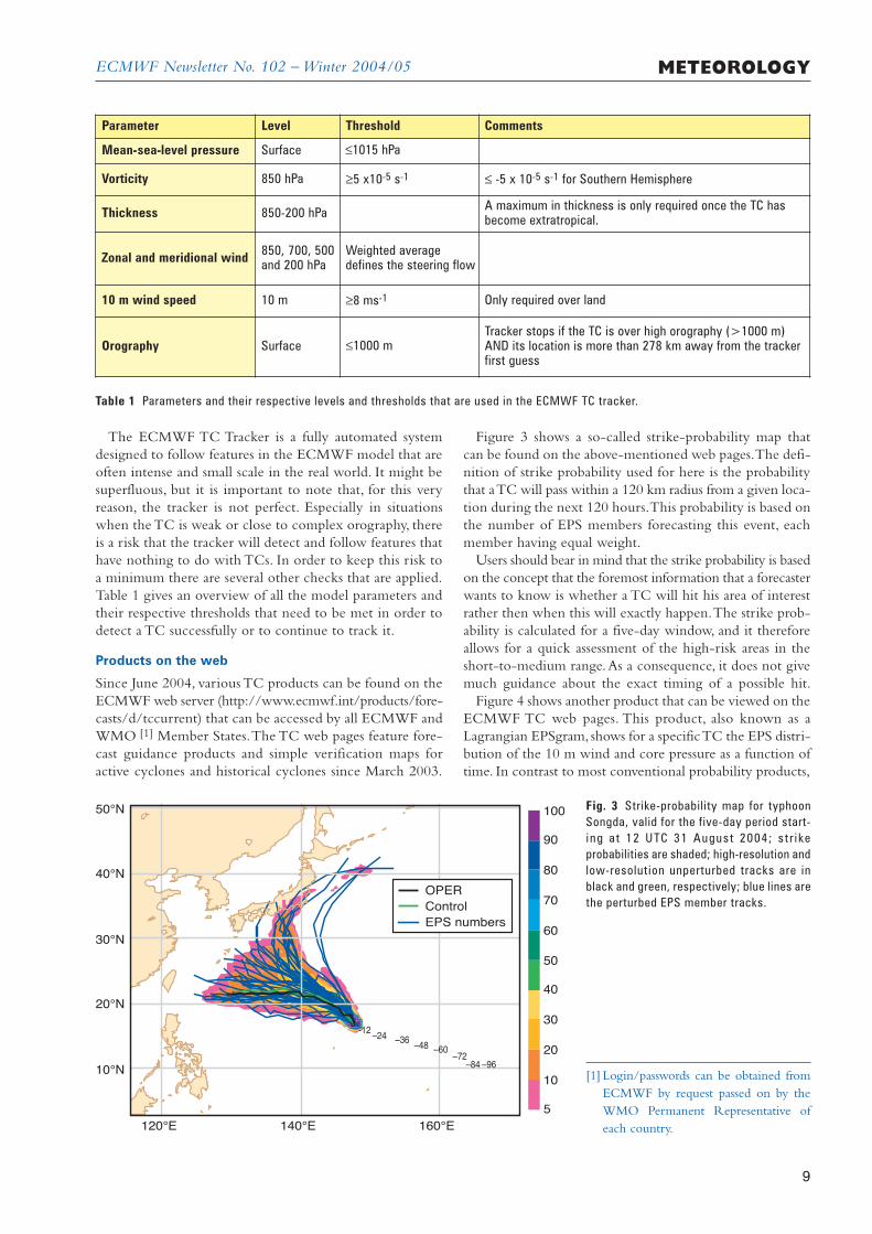
Figure 3 shows a so-called strike-probability map thatcan be found on the above-mentioned web pages.The defi-nition of strike probability used for here is the probabilitythat a TC will pass within a 120 km radius from a given loca-tion during the next 120 hours.This probability is based onthe number of EPS members forecasting this event, eachmember having equal weight.
Users should bear in mind that the strike probability is basedon the concept that the foremost information that a forecasterwants to know is whether a TC will hit his area of interestrather then when this will exactly happen.The strike prob-ability is calculated for a five-day window, and it thereforeallows for a quick assessment of the high-risk areas in theshort-to-medium range.As a consequence, it does not givemuch guidance about the exact timing of a possible hit.
Figure 4 shows another product that can be viewed on theECMWF TC web pages. This product, also known as aLagrangian EPSgram, shows for a specific TC the EPS distri-bution of the 10 m wind and core pressure as a function oftime. In contrast to most conventional probability products,
Parameter Level Threshold Comments
Mean-sea-level pressure Surface ≤1015 hPa
Vorticity 850 hPa ≥5 x10⁻⁵ s-1 ≤ -5 x 10⁻⁵ s-1 for Southern Hemisphere
Thickness 850-200 hPa A maximum in thickness is only required once the TC hasbecome extratropical.
Zonal and meridional wind 850, 700, 500and 200 hPa
Weighted averagedefines the steering flow
10 m wind speed 10 m ≥8 ms-1 Only required over land
Orography Surface ≤1000 mTracker stops if the TC is over high orography (>1000 m)AND its location is more than 278 km away from the trackerfirst guess
Table 1 Parameters and their respective levels and thresholds that are used in the ECMWF TC tracker.
5
10
20
30
40
50
60
70
80
90
100
0-12
–24–36
–48–60
–72–84 –9610°N
20°N
30°N
40°N
50°N
120°E 140°E 160°E
OPERControlEPS numbers
Fig. 3 Strike-probability map for typhoonSongda, valid for the five-day period start-ing a t 12 UTC 31 August 2004; s t r ikeprobabilities are shaded; high-resolution andlow-resolution unperturbed tracks are inblack and green, respectively; blue lines arethe perturbed EPS member tracks.
[1] Login/passwords can be obtained fromECMWF by request passed on by theWMO Permanent Representative ofeach country.
ECMWF Newsletter No. 102 – Winter 2004/05METEOROLOGY
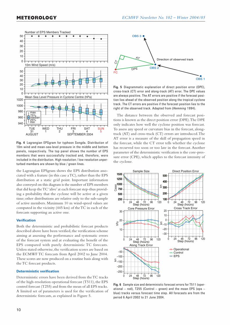
10
the Lagrangian EPSgram shows the EPS distribution asso-ciated with a feature (in this case a TC), rather than the EPSdistribution at a static grid point. Important informationalso conveyed on this diagram is the number of EPS membersthat did keep the TC ‘alive’ at each forecast step-thus provid-ing a probability that the cyclone will be active at a giventime; other distributions are relative only to the sub-sampleof active members. Maximum 10 m wind-speed values arecomputed in the vicinity (445 km) of the TC in each of theforecasts supporting an active one.
Verification
Both the deterministic and probabilistic forecast productsdescribed above have been verified, the verification schemeaiming at assessing the performance and systematic errorsof the forecast system and at evaluating the benefit of theEPS compared with purely deterministic TC forecasts.Unless stated otherwise, the verification scores are based onthe ECMWF TC forecasts from April 2002 to June 2004.These scores are now produced on a routine basis along withthe TC forecast products.
Deterministic verification
Deterministic errors have been derived from the TC tracksof the high-resolution operational forecast (T511), the EPScontrol forecast (T255) and from the mean of all EPS tracks.A limited set of parameters is used for the verification ofdeterministic forecasts, as explained in Figure 5.
Fig. 5 Diagrammatic explanation of direct position error (DPE),cross-track (CT) error and along-track (AT) error. The DPE valuesare always positive. The AT errors are positive if the forecast posi-tion lies ahead of the observed position along the tropical cyclonetrack. The CT errors are positive if the forecast position lies to theright of the observed track. Adapted from (Hemming 1994).
The distance between the observed and forecast posi-tions is known as the direct position error (DPE).The DPEonly indicates how well the cyclone position was forecast.To assess any speed or curvature bias in the forecast, along-track (AT) and cross-track (CT) errors are introduced.TheAT error is a measure of the skill of propagation speed inthe forecast, while the CT error tells whether the cyclonehas recurved too soon or too late in the forecast. Anotherparameter of the deterministic verification is the core-pres-sure error (CPE), which applies to the forecast intensity ofthe cyclone.
Fig. 4 Lagrangian EPSgram for typhoon Songda. Distribution of10m wind and mean-sea-level pressure in the middle and bottompanels, respectively. The top panel shows the number of EPSmembers that were successfully tracked and, therefore, wereincluded in the distribution. High resolution / low resolution unper-turbed members are shown by blue / green lines.
0
10
20
30
40
50Number of EPS Members Tracked
010
203040
50
10m Wind Speed (m/s)
940
960
980
1000
1020
TUE WED THU FRI SAT SUN31
AUGUST1 2 3 4 5
SEPTEMBER 2004
Mean Sea Level Pressure in Cyclone Centre (hPa)
min25%median75%max
FC
OBS 3
OBS 2
OBS 1
AT
CT
DPE
Direction of observed track
250
500
750
1000
1250
1500
100
200
300
400
500
km
250
500
750
1000
1250
1500
100
200
300
400
500
–150
250
500
750
1000
1250
1500
Cases
Sample Size
100
200
300
400
500
Direct Position Error
10
20
30
hPa
Core Pressure Error
0 24 48 72 96 120Step (hours)
0 24 48 72 96 120Step (hours)
0 24 48 72 96 120Step (hours)
0 24 48 72 96 120Step (hours)
0 24 48 72 96 120Step (hours)
–10
–20
–30
0
10
20Cross Track Error
–250
–200
–100
–50
km
km
Along Track Error
ControlOperational
EPS
Fig. 6 Sample size and deterministic forecast errors for T511 (oper-ational – red), T255 (Control – green) and the mean EPS (eps –blue) tracks versus forecast time step. All forecasts are from theperiod 6 April 2002 to 21 June 2004.
ECMWF Newsletter No. 102 – Winter 2004/05 METEOROLOGY
11
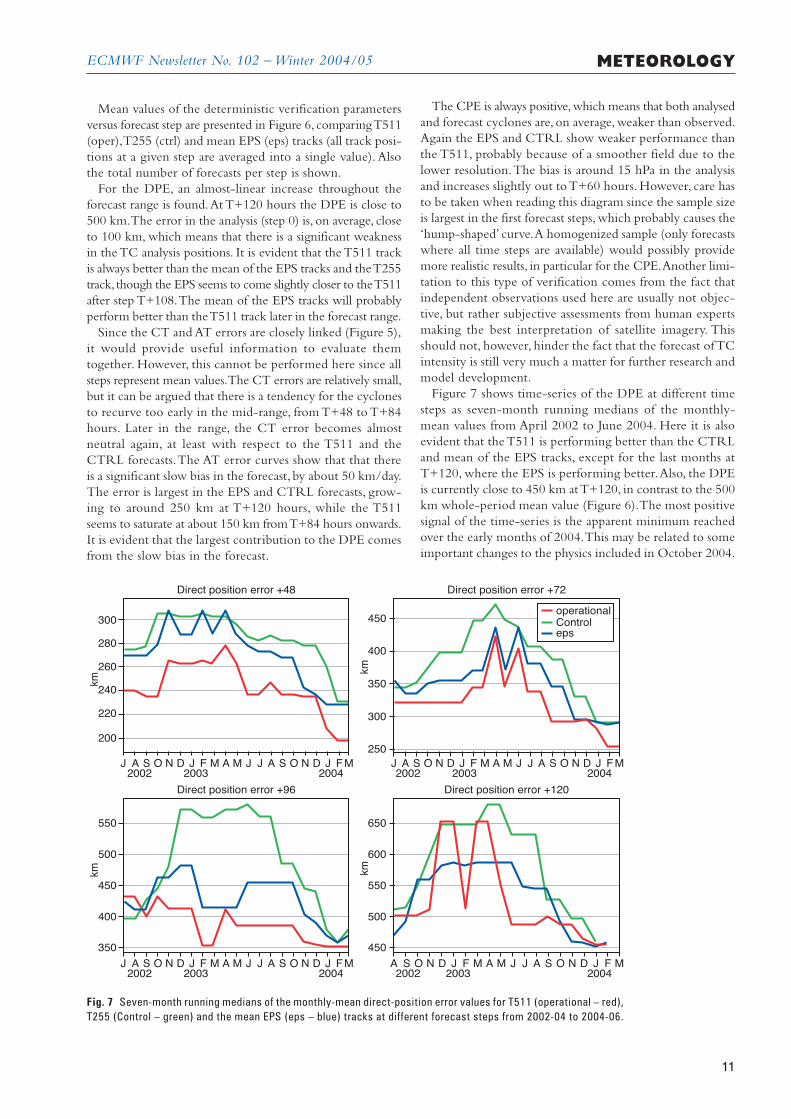
Mean values of the deterministic verification parametersversus forecast step are presented in Figure 6, comparing T511(oper),T255 (ctrl) and mean EPS (eps) tracks (all track posi-tions at a given step are averaged into a single value). Alsothe total number of forecasts per step is shown.
For the DPE, an almost-linear increase throughout theforecast range is found.At T+120 hours the DPE is close to500 km.The error in the analysis (step 0) is, on average, closeto 100 km, which means that there is a significant weaknessin the TC analysis positions. It is evident that the T511 trackis always better than the mean of the EPS tracks and the T255track, though the EPS seems to come slightly closer to the T511after step T+108.The mean of the EPS tracks will probablyperform better than the T511 track later in the forecast range.
Since the CT and AT errors are closely linked (Figure 5),it would provide useful information to evaluate themtogether. However, this cannot be performed here since allsteps represent mean values.The CT errors are relatively small,but it can be argued that there is a tendency for the cyclonesto recurve too early in the mid-range, from T+48 to T+84hours. Later in the range, the CT error becomes almostneutral again, at least with respect to the T511 and theCTRL forecasts.The AT error curves show that that thereis a significant slow bias in the forecast, by about 50 km/day.The error is largest in the EPS and CTRL forecasts, grow-ing to around 250 km at T+120 hours, while the T511seems to saturate at about 150 km from T+84 hours onwards.It is evident that the largest contribution to the DPE comesfrom the slow bias in the forecast.
The CPE is always positive,which means that both analysedand forecast cyclones are, on average, weaker than observed.Again the EPS and CTRL show weaker performance thanthe T511, probably because of a smoother field due to thelower resolution.The bias is around 15 hPa in the analysisand increases slightly out to T+60 hours. However, care hasto be taken when reading this diagram since the sample sizeis largest in the first forecast steps, which probably causes the‘hump-shaped’ curve.A homogenized sample (only forecastswhere all time steps are available) would possibly providemore realistic results, in particular for the CPE.Another limi-tation to this type of verification comes from the fact thatindependent observations used here are usually not objec-tive, but rather subjective assessments from human expertsmaking the best interpretation of satellite imagery. Thisshould not, however, hinder the fact that the forecast of TCintensity is still very much a matter for further research andmodel development.
Figure 7 shows time-series of the DPE at different timesteps as seven-month running medians of the monthly-mean values from April 2002 to June 2004. Here it is alsoevident that the T511 is performing better than the CTRLand mean of the EPS tracks, except for the last months atT+120, where the EPS is performing better.Also, the DPEis currently close to 450 km at T+120, in contrast to the 500km whole-period mean value (Figure 6).The most positivesignal of the time-series is the apparent minimum reachedover the early months of 2004.This may be related to someimportant changes to the physics included in October 2004.
AJ2002
S O N D J2003
F M A M J J A S O N JD2004
AJ2002
S O N D J2003
F M A M J J A S O N JD2004
AJ2002
S O N D J2003
F M A M J J A S O N JD2004 2002
SA O N D J2003
F M A M J J A S O N J
F F
F FD2004
200
220
240
260
280
300
km
km
250
300
350
400
450
Direct position error +72
350
400
450
500
550
km
Direct position error +96
M M
M M
450
500
550
600
650
km
Direct position error +120
Direct position error +48
operationalControleps
Fig. 7 Seven-month running medians of the monthly-mean direct-position error values for T511 (operational – red),T255 (Control – green) and the mean EPS (eps – blue) tracks at different forecast steps from 2002-04 to 2004-06.
ECMWF Newsletter No. 102 – Winter 2004/05METEOROLOGY
12
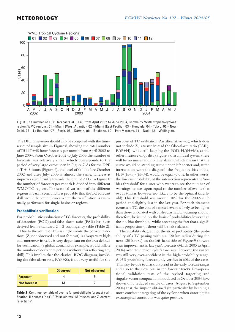
The DPE time-series should also be compared with the time-series of sample size in Figure 8, showing the total numberof T511 T+48 hour forecasts per month from April 2002 toJune 2004. From October 2002 to July 2003 the number offorecasts was relatively small, which corresponds to theperiod of very large errors seen in Figure 7.As for the DPEat T +48 hours (Figure 6), the level of skill before October2002 and after July 2003 is almost the same, whereas itimproves significantly towards the end of 2003. In Figure 8the number of forecasts per month is divided into differentWMO TC regions.The seasonal variation of the differentregions is easily seen, and it is probable that the TC forecastskill would become clearer when the verification is even-tually performed for single basins or regions.
Probabilistic verification
For probabilistic evaluation of TC forecasts, the probabilityof detection (POD) and false-alarm ratio (FAR) has beenderived from a standard 2 × 2 contingency table (Table 2).
Due to the nature of TCs as single events, the correct rejec-tions (Z, not observed and not forecast) is always very highand,moreover, its value is very dependant on the area definedfor verification (a global domain, for example, would inflatethe number of correct rejections without this reflecting anyskill).This implies that the classical ROC diagram, involv-ing the false alarm rate, F/(F+Z), is not very useful for the
Observed Not observed
Forecast H F
Not forecast M Z
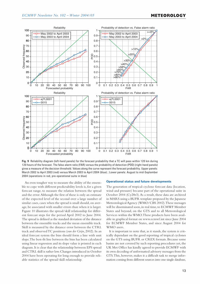
purpose of TC evaluation. An alternative way, which doesnot include Z, is to use instead the false-alarm ratio (FAR),F/(F+H), while still keeping the POD, H/(H+M), as theother measure of quality (Figure 9). In an ideal system therewill be no misses and no false alarms, which means that thecurve would be standing at the upper left corner and, at theintersection with the diagonal, the frequency-bias index,FBI=(H+F)/(H+M),would be equal to one. In other words,the forecast probability at the intersection represents the ‘no-bias threshold’ for a user who wants to see the number ofwarnings he acts upon equal to the number of events thatoccur (this is, however, not likely to be the optimal thresh-old). This threshold was around 30% for the 2002-2003period and slightly less in the last year. For such dramaticevents as a TC, the cost of a missed event is likely to be higherthan those associated with a false alarm.TC warnings should,therefore, be issued on the basis of probabilities lower thanthe ‘no-bias threshold’, while accepting the fact that a signif-icant proportion of them will be false alarms.
The reliability diagram for the strike probability (the prob-ability of a TC passing within a 120 km radius during thenext 120 hours.) on the left-hand side of Figure 9 shows aclear improvement in last year’s forecasts (March 2003 to April2004) over the previous year’s forecasts.However, the systemwas still very over-confident in the high-probability range.A 95% probability forecast only verifies in 60% of the cases.This may be due to a lack of spread in the early forecast rangesand also to the slow bias in the forecast tracks. Pre-opera-tional validation tests of the revised targeting andsingular-vector computation introduced in October 2004 haveshown on a reduced sample of cases (August to September2004) that the impact obtained (in particular by keeping amore consistent targeting of the cyclone when entering theextratropical transition) was quite positive.
01 02 03 04 05 06 07 08 09 10
D
11
MA2002
J J A S O N D J2003
F M A M J J A S O N J2004
F M A M J0
20
40
60
80
100
Cas
es
WMO Tropical Cyclone Regions12
Fig. 8 The number of T511 forecasts at T+48 from April 2002 to June 2004, shown by WMO tropical-cycloneregion. WMO regions: 01 – Miami (West Atlantic), 02 – Miami (East Pacific), 03 – Honolulu, 04 – Tokyo, 05 – NewDelhi, 06 – La Reunion, 07 – Perth, 08 – Darwin, 09 – Brisbane, 10 – Port Moresby, 11 – Nadi, 12 – Wellington.
Table 2 Contingency table of events for probabilistic forecast veri-fication. H denotes ‘hits’, F ‘false alarms’, M ‘misses’ and Z ‘correctrejections’.
ECMWF Newsletter No. 102 – Winter 2004/05 METEOROLOGY
13
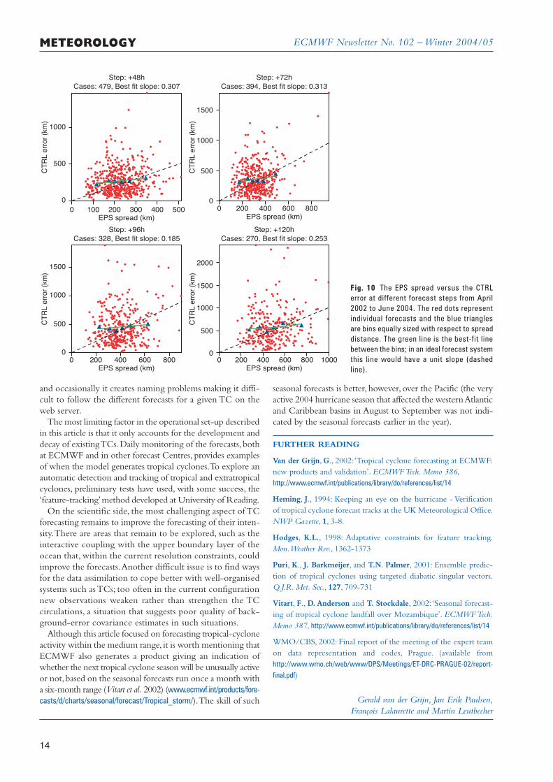
An even tougher way to measure the ability of the ensem-ble to cope with different predictability levels is, for a givenforecast range, to measure the relation between the spreadand the error.Although the first of these is only an estimateof the expected level of the second over a large number ofsimilar cases, cases when the spread is small should, on aver-age, be associated with smaller errors than when it is larger.Figure 10 illustrates the spread/skill relationship for differ-ent forecast steps for the period April 2002 to June 2004.The spread is defined as the standard deviation of the distancebetween the ensemble tracks and the mean ensemble track.Skill is measured by the distance error between the CTRLtrack and observed TC positions (van der Grijn, 2002). In anideal forecast system the bins should form a line with unitslope.The best-fit line between the bins has been calculatedusing linear regression and its slope value is printed in eachdiagram. It is clear that the relationship between EPS spreadand CTRL skill is rather low.Changes introduced in October2004 have been operating for long enough to provide reli-able statistics of the spread/skill relationship.
Operational status and future developments
The generation of tropical-cyclone forecast data (location,wind and pressure) became part of the operational suite inOctober 2004 (Cy28r3).As a result, these data are archivedin MARS using a BUFR template proposed by the JapaneseMeteorological Agency (WMO/CBS 2002).These messageswill be disseminated soon, in real time, to ECMWF MemberStates and beyond, on the GTS and to all MeteorologicalServices within the WMO.These products have been avail-able in graphical format on www.ecmwf.int since June 2004for ECMWF Member States, and since August 2004 forWMO users.
It is important to note that, as it stands, the system is crit-ically dependant on the good reporting of tropical cycloneson the GTS using BUFR or CREX formats. Because somebasins are not covered by such reporting procedures yet, theUK Met Office has kindly agreed to provide ECMWF withits own decoding of unformatted advisory messages from theGTS.This, however, makes it a difficult task to merge infor-mation coming from different sources into one single database,
0 908070605040302010Forecasted probability
0
10
20
30
40
50
60
70
80
90
100
Obs
erve
d fr
eque
ncy
Reliability
0
0.1
0.2
0.3
0.4
0.5
0.6
0.7
0.8
0.9
1
PO
D
Reliability Probability of detection vs. False alarm ratio
Probability of detection vs. False alarm ratio
1
0
10
20
30
40
50
60
70
80
90
100
Obs
erve
d fr
eque
ncy
PO
D
1000
20
40
60
80
100
FAR
>=0%
>0%
>10%
>20%
>30%>40%
>50%>60%
>70%>80%>90%
0 0.1 0.2 0.90.80.70.60.50.40.3 1
0 908070605040302010Forecasted probability
100FAR
0 0.1 0.2 0.90.80.70.60.50.40.3 10
20
40
60
80
100
0
0.1
0.2
0.3
0.4
0.5
0.6
0.7
0.8
0.9
11
May 2003 to April 2004May 2002 to April 2003
May 2003 to April 2004May 2002 to April 2003
0015ej7t,0001
0015ej7t,0001
Fig. 9 Reliability diagram (left-hand panels) for the forecast probability that a TC will pass within 120 km during120 hours of the forecast. The false-alarm ratio (FAR) versus the probability of detection (POD) (right-hand panels)gives a measure of the decision threshold. Values along the curve represent the forecast probability. Upper panels:March 2002 to April 2003 (red) versus March 2003 to April 2004 (blue) ; Lower panels: August to mid-September2004 (operations in red, pre-operational suite in blue)
ECMWF Newsletter No. 102 – Winter 2004/05METEOROLOGY
14
and occasionally it creates naming problems making it diffi-cult to follow the different forecasts for a given TC on theweb server.
The most limiting factor in the operational set-up describedin this article is that it only accounts for the development anddecay of existing TCs. Daily monitoring of the forecasts, bothat ECMWF and in other forecast Centres, provides examplesof when the model generates tropical cyclones.To explore anautomatic detection and tracking of tropical and extratropicalcyclones, preliminary tests have used, with some success, the‘feature-tracking’method developed at University of Reading.
On the scientific side, the most challenging aspect of TCforecasting remains to improve the forecasting of their inten-sity.There are areas that remain to be explored, such as theinteractive coupling with the upper boundary layer of theocean that, within the current resolution constraints, couldimprove the forecasts.Another difficult issue is to find waysfor the data assimilation to cope better with well-organisedsystems such as TCs; too often in the current configurationnew observations weaken rather than strengthen the TCcirculations, a situation that suggests poor quality of back-ground-error covariance estimates in such situations.
Although this article focused on forecasting tropical-cycloneactivity within the medium range, it is worth mentioning thatECMWF also generates a product giving an indication ofwhether the next tropical cyclone season will be unusually activeor not, based on the seasonal forecasts run once a month witha six-month range (Vitart et al. 2002) (www.ecmwf.int/products/fore-casts/d/charts/seasonal/forecast/Tropical_storm/).The skill of such
seasonal forecasts is better, however, over the Pacific (the veryactive 2004 hurricane season that affected the western Atlanticand Caribbean basins in August to September was not indi-cated by the seasonal forecasts earlier in the year).
FURTHER READING
Van der Grijn, G., 2002:‘Tropical cyclone forecasting at ECMWF:new products and validation’. ECMWF Tech. Memo 386,http://www.ecmwf.int/publications/library/do/references/list/14
Heming, J., 1994: Keeping an eye on the hurricane - Verificationof tropical cyclone forecast tracks at the UK Meteorological Office.NWP Gazette, 1, 3-8.
Hodges, K.L., 1998: Adaptative constraints for feature tracking.Mon.Weather Rev., 1362-1373
Puri, K., J. Barkmeijer, and T.N. Palmer, 2001: Ensemble predic-tion of tropical cyclones using targeted diabatic singular vectors.Q.J.R. Met. Soc., 127, 709-731
Vitart, F., D. Anderson and T. Stockdale, 2002: ‘Seasonal forecast-ing of tropical cyclone landfall over Mozambique’. ECMWF Tech.Memo 387, http://www.ecmwf.int/publications/library/do/references/list/14
WMO/CBS, 2002: Final report of the meeting of the expert teamon data representation and codes, Prague. (available fromhttp://www.wmo.ch/web/www/DPS/Meetings/ET-DRC-PRAGUE-02/report-
final.pdf)
0 100 200 300 400 500EPS spread (km)
0
500
1000
CT
RL
erro
r (k
m)
Cases: 479, Best fit slope: 0.307Step: +48h
0
500
1000
1500
Cases: 394, Best fit slope: 0.313Step: +72h
0
500
1000
1500
CT
RL
erro
r (k
m)
CT
RL
erro
r (k
m)
CT
RL
erro
r (k
m)
Cases: 328, Best fit slope: 0.185Step: +96h
0 200 400 600 800 1000EPS spread (km)
0 200 400 600 800EPS spread (km)
0 200 400 600 800EPS spread (km)
0
500
1000
1500
2000
Cases: 270, Best fit slope: 0.253Step: +120h
Fig. 10 The EPS spread versus the CTRLerror at different forecast steps from April2002 to June 2004. The red dots representindividual forecasts and the blue trianglesare bins equally sized with respect to spreaddistance. The green line is the best-fit linebetween the bins; in an ideal forecast systemthis line would have a unit slope (dashedline).
Gerald van der Grijn, Jan Erik Paulsen,François Lalaurette and Martin Leutbecher
ECMWF Newsletter No. 102 – Winter 2004/05 METEOROLOGY
15
The following article from the Turkish Weather Service illustratesthe difficult decisions facing forecasters when they anticipate a severeweather event:When should public warnings be issued? Which organ-isations should be warned? How should they react in the face of asceptical press? How can they ensure that appropriate evasiveactions are taken? The forecast described (based primarily onECMWF predictions) was very successful, and the reaction of thepublic and the authorities was much improved over their responsesto forecasts of a previous snowstorm a few weeks earlier.
The north-western part of Turkey, especially Istanbulwith a population of 10 million, was exposed to asnowstorm between 20-22 January 2004.The Turkish
Met. Service had warned all the authorities and peoplethree days before the event. Unfortunately, however, all thenecessary actions were not taken as required. This failurecaused many people to be affected by the snowstorm andthere were four fatalities.The case was much criticised bythe media. One important question arose:What will we doif the same thing happens again?
8 February 2004 – Forecasting the new snowstorm
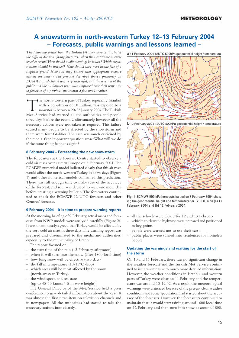
The forecasters at the Forecast Centre started to observe acold air mass over eastern Europe on 8 February 2004.TheECMWF numerical model indicated clearly that this air masswould affect the north-western Turkey in a few days (Figure1), and other numerical models confirmed this prediction.There was still enough time to make sure of the accuracyof the forecast, and so it was decided to wait one more daybefore creating a warning bulletin.The forecasters contin-ued to check the ECMWF 12 UTC forecasts and otherCentres’ forecasts.
9 February 2004 – It is time to prepare warning reports
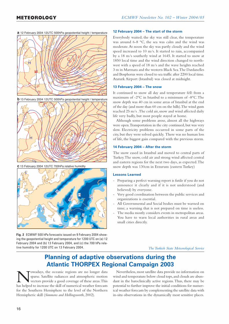
At the morning briefing of 9 February, actual maps and fore-casts from NWP models were analysed carefully (Figure 2).It was unanimously agreed that Turkey would be affected bythe very cold air mass in three days.The warning report wasprepared and disseminated to the media and authorities,especially to the municipality of Istanbul.
The report focused on:- the start time of the rain (12 February, afternoon)- when it will turn into the snow (after 1800 local time)- how long snow will be effective (two days)- the fall in temperature (10-15°C drop)- which areas will be most affected by the snow
(north-western Turkey)- the wind speed and sea state
(up to 45-50 knots, 4-5 m wave height)The General Director of the Met. Service held a press
conference to give detailed information about the case. Itwas almost the first news item on television channels andin newspapers. All the authorities had started to take thenecessary actions immediately.
A snowstorm in north-western Turkey 12–13 February 2004– Forecasts, public warnings and lessons learned –
H
516
528
540
552
564
H
516
528
540
552
564
L
L W
W
C
C
-45
-40
-35
-30
-25
-20-20
-20
-15
L
L
WW
C
C
-45
-40
-35
-30
-25
-20
-20
-15
a 11 February 2004 12UTC 500hPa geopotential height / temperature
b 12 February 2004 12UTC 500hPa geopotential height / temperature
Fig. 1 ECMWF 500 hPa forecasts issued on 8 February 2004 show-ing the geopotential height and temperature for 1200 UTC on (a) 11February 2004 and (b) 12 February 2004.
- all the schools were closed for 12 and 13 February- vehicles to clear the highways were prepared and positioned
to key points- people were warned not to use their cars.- public places were turned into residences for homeless
people
Updating the warnings and waiting for the start ofthe storm
On 10 and 11 February, there was no significant change inthe weather forecast and the Turkish Met Service contin-ued to issue warnings with much more detailed information.However, the weather conditions in Istanbul and westernparts of Turkey were clear on 11 February and the temper-ature was around 10-12 °C.As a result, the meteorologicalwarnings were criticized because of the present clear weatherconditions and some speculation had started about the accu-racy of the forecasts. However, the forecasters continued tomaintain that it would start raining around 1600 local timeon 12 February and then turn into snow at around 1800.
ECMWF Newsletter No. 102 – Winter 2004/05METEOROLOGY
16
12 February 2004 – The start of the storm
Everybody waited; the sky was still clear, the temperaturewas around 6-8 °C, the sea was calm and the wind wasmoderate.At noon the sky was partly cloudy and the windspeed increased to 10 m/s. It started to rain, accompaniedby a 18 m/s southerly wind at 1645. It started to snow at1850 local time and the wind direction changed to north-west with a speed of 18 m/s and the wave heights reached3 m in Marmara and the western Black Sea.The Dardanellesand Bosphorus were closed to sea traffic after 2200 local time.Ataturk Airport (Istanbul) was closed at midnight.
13 February 2004 – The snow
It continued to snow all day and temperature fell: from amaximum of -2°C in Istanbul to a minimum of -8°C.Thesnow depth was 40 cm in some areas of Istanbul at the endof the day (and more than 60 cm on the hills).The wind gustsreached 25 m/s .The cold air, snow and wind affected dailylife very badly, but most people stayed at home.
Although some problems arose, almost all the highwayswere open.Transportation in the city continued, but was veryslow. Electricity problems occurred in some parts of thecity, but they were solved quickly. There was no human lossof life, the biggest gain compared with the previous storm.
14 February 2004 – After the storm
The snow eased in Istanbul and moved to central parts ofTurkey.The snow, cold air and strong wind affected centraland eastern regions for the next two days, as expected.Thesnow depth was 130cm in Erzurum (eastern Turkey)
Lessons Learned
- Preparing a perfect warning report is futile if you do notannounce it clearly and if it is not understood (andbelieved) by everyone.
- Very good coordination between the public services andorganizations is essential.
- All Governmental and Social bodies must be warned ontime; a warning that is not prepared on time is useless.
- The media mostly considers events in metropolitan areas.You have to warn local authorities in rural areas andsmall cities directly.
L
W
C
C
-45
-40
-35
-30
-25
-20-20
-20
-15
L
W
W
C
-40-35
-35
-30
-25
-20
-20 -15
H
516
528
540
552
564
H
516
528
528
540
552564
564
576576
H
H
LL
L
50
50
50
50
5050
70
70
70
70
70
90
90
90
a 12 February 2004 12UTC 500hPa geopotential height / temperature
b 13 February 2004 12UTC 500hPa geopotential height / temperature
c 13 February 2004 12UTC 700hPa relative humidity
Fig. 2 ECMWF 500 hPa forecasts issued on 9 February 2004 show-ing the geopotential height and temperature for 1200 UTC on (a) 12February 2004 and (b) 13 February 2004, and (c) the 700 hPa rela-tive humidity for 1200 UTC on 13 February 2004. The Turkish State Meteorological Service
Nowadays, the oceanic regions are no longer datasparse. Satellite radiances and atmospheric motionvectors provide a good coverage of these areas.This
has helped to increase the skill of numerical weather forecastsfor the Southern Hemisphere to the level of the NorthernHemispheric skill (Simmons and Hollingsworth, 2002).
Nevertheless, most satellite data provide no information onwind and temperature below cloud tops, and clouds are abun-dant in the baroclinically active regions.Thus, there may bepotential to further improve the initial conditions for numer-ical weather forecasts by complementing the satellite data within-situ observations in the dynamically most sensitive places.
Planning of adaptive observations during theAtlantic THORPEX Regional Campaign 2003
ECMWF Newsletter No. 102 – Winter 2004/05
17
METEOROLOGY
The philosophy of adaptive observations (or targeted obser-vations) is to economise observational resources by deployingadditional observations only in those regions where they arelikely to be most important for a specific forecast, i.e. a partic-ular verification region of a few million square kilometres anda specific forecast range of 1-3 days.The process of planningadaptive observations involves several steps. First, verificationregions and forecast ranges are selected for which a forecastimprovement is desired.This step is referred to here as the caseselection.Second, the regions of the atmosphere are predictedwhere improved initial conditions are likely to yield thelargest improvement of the specific forecast.These geographicregions are referred to as sensitive areas. Third, the actualdecisions about the deployment of additional observations aremade, given the sensitive-area predictions and the operationalconstraints.The third step has to take place some time beforethe additional observations are taken. Depending on theprocedure for a particular observation type, the required gapbetween the time of the decision and the observing time isbetween a few hours and two days – up to two days arerequired, for instance, to arrange for a research aircraft todeploy dropsondes, because of air traffic control constraints.
The Atlantic THORPEX Regional Campaign 2003 (A-TReC,see also http://www.wmo.int/thorpex/atlantic_ob_system.html)was an international experiment with a special observingperiod from 13 October to 12 December 2003.The primarygoal of A-TReC was to demonstrate that several differentobserving platforms could be adapted in real time with thegoal to improve operational weather forecasts for Europe.A-TReC is the first observation targeting exercise over theAtlantic with an operational flavour. Initial experience onobservation targeting for NWP was gathered during theFronts and Atlantic Storm-Track Experiment (FASTEX) in1997. Since then, observation-targeting activities took placeevery year over the eastern Pacific. The Winter StormReconnaissance Programme run by the National Centers forEnvironmental Prediction (NCEP) has had operational statussince 2001. In addition, some experience has been obtainedwith adaptive observations in the context of tropical cyclonesin the Atlantic.
The European participation in A-TReC was managedby EUCOS (the EUMETNET Composite ObservingSystem) under the responsibility of the Met Office.The A-TReC operations centre was located at the MetOffice in Exeter, and activities were coordinated throughtwo telephone conferences at 09 UTC and 16 UTC daily.ECMWF was involved in the case selection and in theprediction of sensitive areas for A-TReC. Maps of thepredicted sensitive areas were made available in realtime to A-TReC participants through a web site (nowat http://www.ecmwf.int/research/predictability/adaptive_obs/)hosted at ECMWF. In addition, the sensitive-area predic-tions from Météo-France and the Met Office weretransmitted to ECMWF, and were also displayed on theweb site in the same graphical format as the ECMWFpredictions.
Several people in ECMWF’s Meteorological Applications,Data & Services and Meteorological Operations Sections
provided the technical support to set up the suites for thereal-time sensitive-area prediction, its MARS archive, the website and the A-TReC observation database.
Additional observations
A-TReC is the first field campaign in which multipleobserving systems were targeted in order to improve fore-casts for specific weather events.During part of the campaign,up to three research aircraft capable of deploying dropson-des were available:The DLR Falcon was based in Keflavik(Iceland) from 13 to 22 November.The Gulfstream IV fromNOAA was operating out of St. Johns (Newfoundland)from 13 November to 11 December.The Citation from theUniversity of North Dakota was based in Bangor (Maine,USA) from 23 November to 12 December.
Additional radiosondes were launched in Europe,Greenlandand Canada at 18 UTC on request from the A-TReC obser-vation control centre in Exeter. Further additional soundingswere made by selected vessels of the ASAP fleet at 15 UTCand 21 UTC on request from Exeter. Data transmission wasactivated on additional E-AMDAR aircraft. For all theseplatforms of the routine observing network, requests weremade if additional observations could be obtained close to,or in, the sensitive areas. Moreover, additional drifting buoyswere released before A-TReC in the Labrador and Biscayareas. Supplementary atmospheric motion vectors wereobtained from GOES-East and Meteosat rapid scans overregions centred on the sensitive areas.
Case selection
The 09 UTC teleconference was dedicated to the case selec-tion. Forecasters from the Met Office, Météo-France andECMWF (the time difference precluded participation fromthe US and Canada) joined together to discuss and select rele-vant meteorological situations potentially affecting Europe orthe North American east coast in the coming days.The selec-tion criteria were based mainly on three factors: (a) to addresspotentially hazardous weather events, (b) to focus on cases inwhich an enhanced uncertainty was evident, (c) to selectcases only in the medium-range with a forecast range between3 and 5 days. Although the aim was to improve one- tothree-day forecast, it was necessary to take into account alsothe 48-hour notice required by some observation providers.
Every day, each participant prepared a document contain-ing a brief meteorological description and supporting materialfor an eventual request.The documents were posted on anFTP site hosted by ECMWF ready to be discussed duringthe morning conference (see Figure 1). Since each Centrebased its request on different models, according to its ownjudgement, it was possible to have a good estimate of theforecast uncertainty. In addition, ECMWF provided a set ofoperational products on a dedicated web page with partic-ular emphasis on EPS-derived products (ensemble mean,spread, individual forecasts, probabilities, Extreme ForecastIndex). Once a decision was reached and a case selected, theverification area, the date and the time were used as inputfor the sensitive-area computations to be discussed on thesame day at the 16 UTC conference.
ECMWF Newsletter No. 102 – Winter 2004/05
18
METEOROLOGY
Discussions were useful and often instructive,being enrichedby different experiences and knowledge from differentCentres. Most of the time, agreement on the cases was easilyreached in the allocated time of 30 minutes.However, in duecourse,we noticed that the apparent uncertainty in the fore-cast at day 3–5 was quite often drastically reduced by the timeadditional observations were made (one to three days beforeverification time).This somehow reduced, a posteriori, theneed for additional observations in many cases. It wouldhave been appropriate to cancel many of the previouslyselected cases due to a more predictable situation as theobservation time approached. In other words: adaptive observ-ing techniques might be more successful if the time to alertkey observation providers could be shortened.
Sensitive-area predictions
In order to select optimal locations for a set of additionalobservations, one has to be able to quantify the expectedimpact of additional observations on the forecast uncer-tainty.To estimate the expected impact, it is necessary to knowthe statistics of initial-condition errors, how the initial-condition errors change due to the assimilation of additionalobservations, and about the perturbation dynamics fromthe assimilation time to the forecast verification time.Approximate techniques for determining the sensitive regionsare either adjoint based (singular vectors and adjoint sensi-tivities) or are based on a linear diagnosis of ensembleforecasts (e.g. Ensemble Transform Kalman Filter; ETKF) -see, for example, Leutbecher (2003) and references therein.
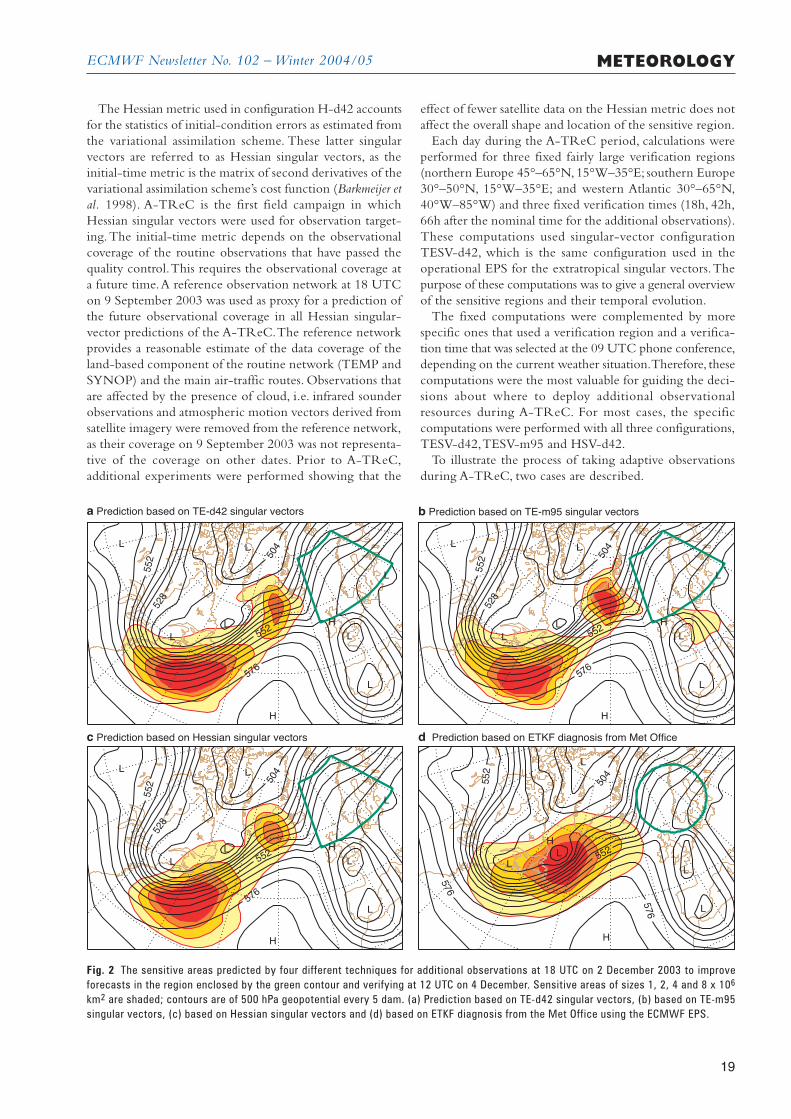
The Met Office based their predictions on EnsembleTransform Kalman Filter diagnostics of the ECMWF ensem-ble. Météo-France and ECMWF based their sensitive-areapredictions on singular vectors.These sensitive-area predic-tions have been archived in MARS:class=to, stream=seap, expver=11, origin=ecmf/lfpw/egrr# ECMWF, MF, UKMO
NCEP (using the Ensemble Transform Kalman Filter oncombined NCEP and ECMWF ensembles) and the NavyResearch Laboratory (NRL) (with singular vectors andobservation sensitivity) also provided targeting guidance,which was displayed on their own web sites.
ECMWF predictions
All singular-vector computations at ECMWF used a trajec-tory starting from the 66-hour forecast valid at the nominalobserving time for the additional observations (18 UTC).Thesensitive-area predictions were ready before 15 UTC, that is,in time for the 16 UTC phone conference and around twodays before the targeted observations were taken. Singularvectors were computed in three different configurations togive an indication of how sensitive the predictions are to thechoice of the initial time metric and to the representationof dynamics and physics in the tangent-linear model (Table1). Configurations TE-d42 and TE-m95 used the total-energy metric both at initial and final time whereasconfiguration H-d42 used the Hessian metric at initial timeand the total-energy metric at final time.A dry tangent-linearmodel at spectral truncation T42 was used in configurationsTE-d42 and H-d42. Singular vectors in configuration TE-m95 were computed with a TL95 moist tangent-linear model.
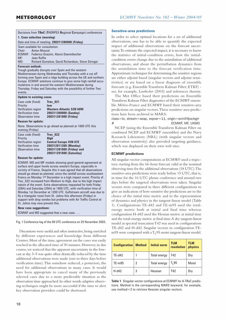
Decisions from TReC (THORPEX Regional Campaign) conferences1. Case selection (morning)Date and time of meeting: 200311280900 (Friday)Team available for consultation:Chair: Anton MuscatECMWF: Federico Grazzini, Alexis DoerenbecherMF: Jean RuffieMO: Richard Dumelow, David Richardson, Steve StringerForecast outlook:Trough gradually disrupts over Spain and the westernMediterranean during Wednesday and Thursday with a cut offforming over Spain and a ridge building across the UK and northernEurope. ECMWF solutions continue to give some high rainfall accu-mulations in and around the western Mediterranean duringThursday, Friday and Saturday with the possibility of further Trecevents.Update to existing casesCase code (fixed) Trec_021Priority lowVerification region Western Atlantic 52N 60WVerification time 200311300000 (Sunday)Observation time 200311281800 (Friday)Reason for update:None. Observations to go ahead as planned at 1800 UTC thisevening (Friday)Case code (fixed) Trec_022Priority HighVerification region Central Europe 45N 07EVerification time 200312011200 (Monday)Observation time 200311281800 (Friday) and
200311291800 (Saturday)Reason for update:ECMWF, MO and MF models showing good general agreement atsurface and upper levels across western Europe, especially invicinity of France. Despite this it was agreed that all observationsshould go ahead as planned, since the rainfall across southeasternFrance on Monday 1st December is a high impact event. Priority ofTrec_022 increased from Medium to High, due to the high impactnature of the event. Extra observations requested for both Friday(28th) and Saturday (29th) at 1800 UTC, with verification time ofMonday 1st December at 1200 UTC. Gulfstream aircraft was due tofly a triangular route from St. Johns this afternoon (Friday) insupport with drop sondes but problems with Air Traffic Control atSt. Johns may now prevent this.New case suggestions:ECMWF and MO suggested that a new case . . .
Fig. 1 Conference log of the 09 UTC conference on 25 November 2003.
Configuration Method Initial norm TLMresolution
TLMphysics
TE-d42 1 Total energy T42 Dry
TE-m95 2 Total energy TL95 Moist
H-d42 3 Hessian T42 Dry
Table 1 Singular-vector configurations at ECMWF for A-TReC predic-tions. Method is the corresponding MARS keyword; for example,use method=3 to retrieve Hessian singular vectors.
ECMWF Newsletter No. 102 – Winter 2004/05
19
METEOROLOGY
The Hessian metric used in configuration H-d42 accountsfor the statistics of initial-condition errors as estimated fromthe variational assimilation scheme. These latter singularvectors are referred to as Hessian singular vectors, as theinitial-time metric is the matrix of second derivatives of thevariational assimilation scheme’s cost function (Barkmeijer etal. 1998). A-TReC is the first field campaign in whichHessian singular vectors were used for observation target-ing.The initial-time metric depends on the observationalcoverage of the routine observations that have passed thequality control.This requires the observational coverage ata future time.A reference observation network at 18 UTCon 9 September 2003 was used as proxy for a prediction ofthe future observational coverage in all Hessian singular-vector predictions of the A-TReC.The reference networkprovides a reasonable estimate of the data coverage of theland-based component of the routine network (TEMP andSYNOP) and the main air-traffic routes. Observations thatare affected by the presence of cloud, i.e. infrared sounderobservations and atmospheric motion vectors derived fromsatellite imagery were removed from the reference network,as their coverage on 9 September 2003 was not representa-tive of the coverage on other dates. Prior to A-TReC,additional experiments were performed showing that the
effect of fewer satellite data on the Hessian metric does notaffect the overall shape and location of the sensitive region.
Each day during the A-TReC period, calculations wereperformed for three fixed fairly large verification regions(northern Europe 45°–65°N, 15°W–35°E; southern Europe30°–50°N, 15°W–35°E; and western Atlantic 30°–65°N,40°W–85°W) and three fixed verification times (18h, 42h,66h after the nominal time for the additional observations).These computations used singular-vector configurationTESV-d42, which is the same configuration used in theoperational EPS for the extratropical singular vectors.Thepurpose of these computations was to give a general overviewof the sensitive regions and their temporal evolution.
The fixed computations were complemented by morespecific ones that used a verification region and a verifica-tion time that was selected at the 09 UTC phone conference,depending on the current weather situation.Therefore, thesecomputations were the most valuable for guiding the deci-sions about where to deploy additional observationalresources during A-TReC. For most cases, the specificcomputations were performed with all three configurations,TESV-d42,TESV-m95 and HSV-d42.
To illustrate the process of taking adaptive observationsduring A-TReC, two cases are described.
H
H
L
L
L L
L
L
L
504
528
552
552
576
aÊPrediction based on TE-d42 singular vectors
H
H
L
L
L L
L
L
L
504
528
552
552
576
bÊPrediction based on TE-m95 singular vectors
H
H
L
L
L L
L
L
L
504
528
552
552
576
cÊPrediction based on Hessian singular vectors
H
H
L
LL
L
L
504
552
552
576
576
d Prediction based on ETKF diagnosis from Met Office
Fig. 2 The sensitive areas predicted by four different techniques for additional observations at 18 UTC on 2 December 2003 to improveforecasts in the region enclosed by the green contour and verifying at 12 UTC on 4 December. Sensitive areas of sizes 1, 2, 4 and 8 x 10⁶
km2 are shaded; contours are of 500 hPa geopotential every 5 dam. (a) Prediction based on TE-d42 singular vectors, (b) based on TE-m95singular vectors, (c) based on Hessian singular vectors and (d) based on ETKF diagnosis from the Met Office using the ECMWF EPS.
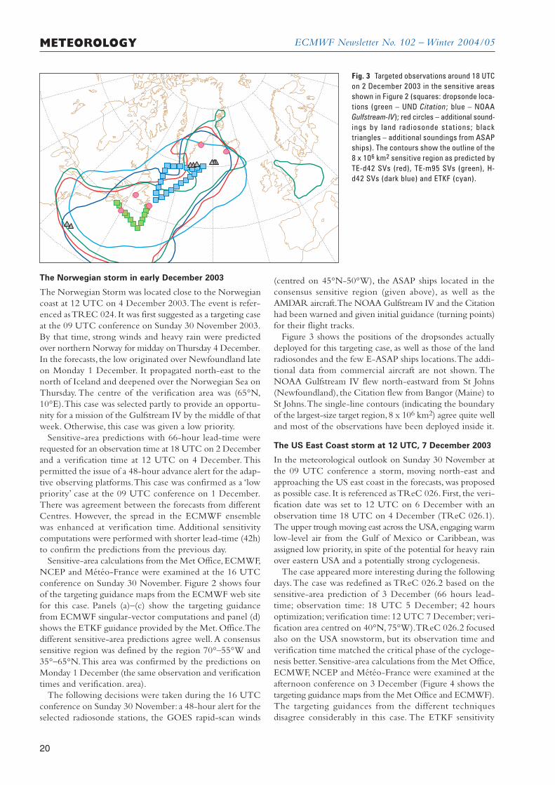
ECMWF Newsletter No. 102 – Winter 2004/05
20
METEOROLOGY
The Norwegian storm in early December 2003
The Norwegian Storm was located close to the Norwegiancoast at 12 UTC on 4 December 2003.The event is refer-enced as TREC 024. It was first suggested as a targeting caseat the 09 UTC conference on Sunday 30 November 2003.By that time, strong winds and heavy rain were predictedover northern Norway for midday on Thursday 4 December.In the forecasts, the low originated over Newfoundland lateon Monday 1 December. It propagated north-east to thenorth of Iceland and deepened over the Norwegian Sea onThursday. The centre of the verification area was (65°N,10°E).This case was selected partly to provide an opportu-nity for a mission of the Gulfstream IV by the middle of thatweek. Otherwise, this case was given a low priority.
Sensitive-area predictions with 66-hour lead-time wererequested for an observation time at 18 UTC on 2 Decemberand a verification time at 12 UTC on 4 December. Thispermitted the issue of a 48-hour advance alert for the adap-tive observing platforms.This case was confirmed as a ‘lowpriority’ case at the 09 UTC conference on 1 December.There was agreement between the forecasts from differentCentres. However, the spread in the ECMWF ensemblewas enhanced at verification time. Additional sensitivitycomputations were performed with shorter lead-time (42h)to confirm the predictions from the previous day.
Sensitive-area calculations from the Met Office, ECMWF,NCEP and Météo-France were examined at the 16 UTCconference on Sunday 30 November. Figure 2 shows fourof the targeting guidance maps from the ECMWF web sitefor this case. Panels (a)–(c) show the targeting guidancefrom ECMWF singular-vector computations and panel (d)shows the ETKF guidance provided by the Met. Office.Thedifferent sensitive-area predictions agree well. A consensussensitive region was defined by the region 70°–55°W and35°–65°N.This area was confirmed by the predictions onMonday 1 December (the same observation and verificationtimes and verification. area).
The following decisions were taken during the 16 UTCconference on Sunday 30 November: a 48-hour alert for theselected radiosonde stations, the GOES rapid-scan winds
(centred on 45°N-50°W), the ASAP ships located in theconsensus sensitive region (given above), as well as theAMDAR aircraft.The NOAA Gulfstream IV and the Citationhad been warned and given initial guidance (turning points)for their flight tracks.
Figure 3 shows the positions of the dropsondes actuallydeployed for this targeting case, as well as those of the landradiosondes and the few E-ASAP ships locations.The addi-tional data from commercial aircraft are not shown. TheNOAA Gulfstream IV flew north-eastward from St Johns(Newfoundland), the Citation flew from Bangor (Maine) toSt Johns.The single-line contours (indicating the boundaryof the largest-size target region, 8 x 10⁶ km2) agree quite welland most of the observations have been deployed inside it.
The US East Coast storm at 12 UTC, 7 December 2003
In the meteorological outlook on Sunday 30 November atthe 09 UTC conference a storm, moving north-east andapproaching the US east coast in the forecasts, was proposedas possible case. It is referenced as TReC 026. First, the veri-fication date was set to 12 UTC on 6 December with anobservation time 18 UTC on 4 December (TReC 026.1).The upper trough moving east across the USA,engaging warmlow-level air from the Gulf of Mexico or Caribbean, wasassigned low priority, in spite of the potential for heavy rainover eastern USA and a potentially strong cyclogenesis.
The case appeared more interesting during the followingdays.The case was redefined as TReC 026.2 based on thesensitive-area prediction of 3 December (66 hours lead-time; observation time: 18 UTC 5 December; 42 hoursoptimization; verification time: 12 UTC 7 December; veri-fication area centred on 40°N, 75°W).TReC 026.2 focusedalso on the USA snowstorm, but its observation time andverification time matched the critical phase of the cycloge-nesis better. Sensitive-area calculations from the Met Office,ECMWF, NCEP and Météo-France were examined at theafternoon conference on 3 December (Figure 4 shows thetargeting guidance maps from the Met Office and ECMWF).The targeting guidances from the different techniquesdisagree considerably in this case. The ETKF sensitivity
Fig. 3 Targeted observations around 18 UTCon 2 December 2003 in the sensitive areasshown in Figure 2 (squares: dropsonde loca-tions (green – UND Citation; blue – NOAAGulfstream-IV); red circles – additional sound-ings by land radiosonde stations; blacktriangles – additional soundings from ASAPships). The contours show the outline of the8 x 106 km2 sensitive region as predicted byTE-d42 SVs (red), TE-m95 SVs (green), H-d42 SVs (dark blue) and ETKF (cyan).
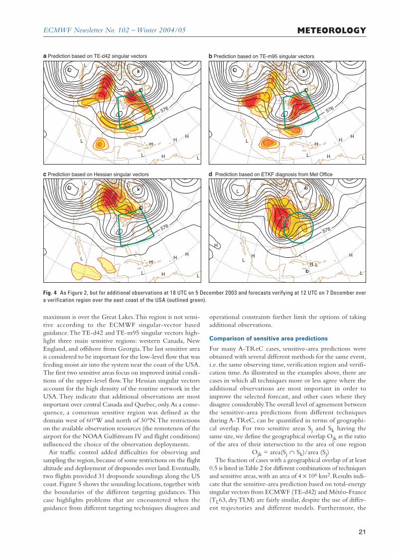
ECMWF Newsletter No. 102 – Winter 2004/05
21
METEOROLOGY
HH
H
H
LLL
L
L
L
L
L
576
HH
H
H
LLL
L
L
L
L
L
576
HH
H
H
LLL
L
L
L
L
L
576
H
HH
H
LL
L
L
LL
L
576
aÊPrediction based on TE-d42 singular vectors bÊPrediction based on TE-m95 singular vectors
cÊPrediction based on Hessian singular vectors d Prediction based on ETKF diagnosis from Met Office
Fig. 4 As Figure 2, but for additional observations at 18 UTC on 5 December 2003 and forecasts verifying at 12 UTC on 7 December overa verification region over the east coast of the USA (outlined green).
maximum is over the Great Lakes.This region is not sensi-tive according to the ECMWF singular-vector basedguidance.The TE-d42 and TE-m95 singular vectors high-light three main sensitive regions: western Canada, NewEngland, and offshore from Georgia.The last sensitive areais considered to be important for the low-level flow that wasfeeding moist air into the system near the coast of the USA.The first two sensitive areas focus on improved initial condi-tions of the upper-level flow.The Hessian singular vectorsaccount for the high density of the routine network in theUSA. They indicate that additional observations are mostimportant over central Canada and Quebec, only.As a conse-quence, a consensus sensitive region was defined as thedomain west of 60°W and north of 30°N.The restrictionson the available observation resources (the remoteness of theairport for the NOAA Gulfstream IV and flight conditions)influenced the choice of the observation deployments.
Air traffic control added difficulties for observing andsampling the region, because of some restrictions on the flightaltitude and deployment of dropsondes over land. Eventually,two flights provided 31 dropsonde soundings along the UScoast. Figure 5 shows the sounding locations, together withthe boundaries of the different targeting guidances. Thiscase highlights problems that are encountered when theguidance from different targeting techniques disagrees and
operational constraints further limit the options of takingadditional observations.
Comparison of sensitive area predictions
For many A-TReC cases, sensitive-area predictions wereobtained with several different methods for the same event,i.e. the same observing time, verification region and verifi-cation time. As illustrated in the examples above, there arecases in which all techniques more or less agree where theadditional observations are most important in order toimprove the selected forecast, and other cases where theydisagree considerably.The overall level of agreement betweenthe sensitive-area predictions from different techniquesduring A-TReC, can be quantified in terms of geographi-cal overlap. For two sensitive areas Sj and Sk having thesame size,we define the geographical overlap Ojk as the ratioof the area of their intersection to the area of one region
Ojk = area(Sj ∩ Sk)/area (Sj)The fraction of cases with a geographical overlap of at least
0.5 is listed in Table 2 for different combinations of techniquesand sensitive areas,with an area of 4 × 10⁶ km2.Results indi-cate that the sensitive-area prediction based on total-energysingular vectors from ECMWF (TE-d42) and Météo-France(TL63, dry TLM) are fairly similar, despite the use of differ-ent trajectories and different models. Furthermore, the
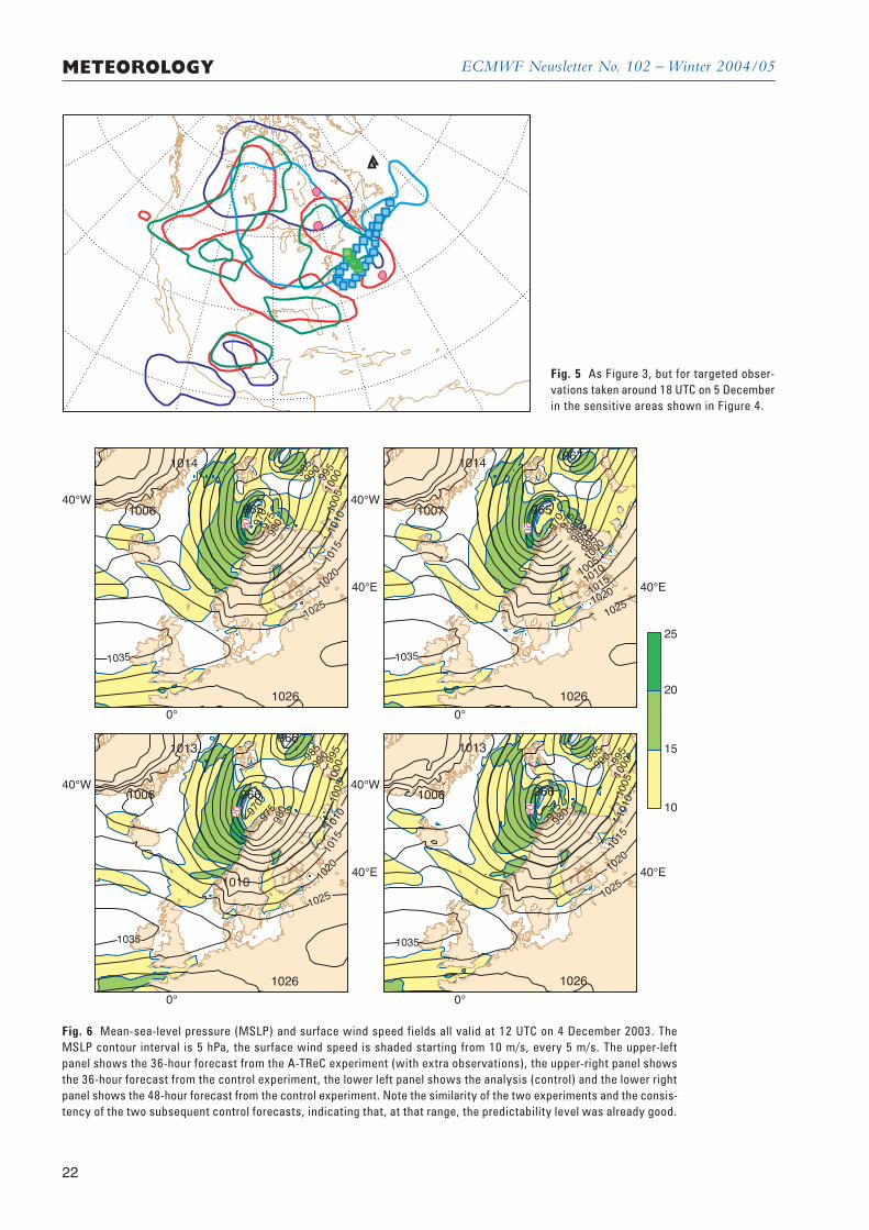
ECMWF Newsletter No. 102 – Winter 2004/05
22
METEOROLOGY
Fig. 5 As Figure 3, but for targeted obser-vations taken around 18 UTC on 5 Decemberin the sensitive areas shown in Figure 4.
20
9651006
1014
1026
970
975
980
985
990
995
1000
1005
1010
1015
1020
1025
1035
40°W
0°
40°E
10
15
20
25
20
965
967
1007
1014
1026
1035
40°W
0°
40°E
20
966
966
1006
1010
1013
1026
970
975
980
985
990 995
1000
1005
1010
1015
1020
1025
1035
40°W
0°
40°E
20
9661006
1013
1026
975
980
985
990 99
510
001005
1010
1015
1020
1025
1035
40°W
0°
40°E
10251020101510101005100099
5900
98598
0975
970
Fig. 6 Mean-sea-level pressure (MSLP) and surface wind speed fields all valid at 12 UTC on 4 December 2003. TheMSLP contour interval is 5 hPa, the surface wind speed is shaded starting from 10 m/s, every 5 m/s. The upper-leftpanel shows the 36-hour forecast from the A-TReC experiment (with extra observations), the upper-right panel showsthe 36-hour forecast from the control experiment, the lower left panel shows the analysis (control) and the lower rightpanel shows the 48-hour forecast from the control experiment. Note the similarity of the two experiments and the consis-tency of the two subsequent control forecasts, indicating that, at that range, the predictability level was already good.
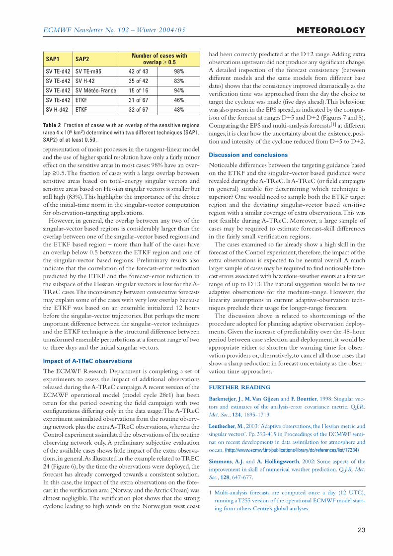
ECMWF Newsletter No. 102 – Winter 2004/05
23
METEOROLOGY
representation of moist processes in the tangent-linear modeland the use of higher spatial resolution have only a fairly minoreffect on the sensitive areas in most cases: 98% have an over-lap ≥0.5.The fraction of cases with a large overlap betweensensitive areas based on total-energy singular vectors andsensitive areas based on Hessian singular vectors is smaller butstill high (83%).This highlights the importance of the choiceof the initial-time norm in the singular-vector computationfor observation-targeting applications.
However, in general, the overlap between any two of thesingular-vector based regions is considerably larger than theoverlap between one of the singular-vector based regions andthe ETKF based region – more than half of the cases havean overlap below 0.5 between the ETKF region and one ofthe singular-vector based regions. Preliminary results alsoindicate that the correlation of the forecast-error reductionpredicted by the ETKF and the forecast-error reduction inthe subspace of the Hessian singular vectors is low for the A-TReC cases.The inconsistency between consecutive forecastsmay explain some of the cases with very low overlap becausethe ETKF was based on an ensemble initialized 12 hoursbefore the singular-vector trajectories.But perhaps the moreimportant difference between the singular-vector techniquesand the ETKF technique is the structural difference betweentransformed ensemble perturbations at a forecast range of twoto three days and the initial singular vectors.
Impact of A-TReC observations
The ECMWF Research Department is completing a set ofexperiments to assess the impact of additional observationsreleased during the A-TReC campaign.A recent version of theECMWF operational model (model cycle 28r1) has beenrerun for the period covering the field campaign with twoconfigurations differing only in the data usage:The A-TReCexperiment assimilated observations from the routine observ-ing network plus the extra A-TReC observations,whereas theControl experiment assimilated the observations of the routineobserving network only. A preliminary subjective evaluationof the available cases shows little impact of the extra observa-tions, in general.As illustrated in the example related to TREC24 (Figure 6),by the time the observations were deployed, theforecast has already converged towards a consistent solution.In this case, the impact of the extra observations on the fore-cast in the verification area (Norway and the Arctic Ocean) wasalmost negligible.The verification plot shows that the strongcyclone leading to high winds on the Norwegian west coast
SAP1 SAP2 Number of cases withoverlap ≥ 0.5
SV TE-d42 SV TE-m95 42 of 43 98%
SV TE-d42 SV H-42 35 of 42 83%
SV TE-d42 SV Météo-France 15 of 16 94%
SV TE-d42 ETKF 31 of 67 46%
SV H-d42 ETKF 32 of 67 48%
had been correctly predicted at the D+2 range.Adding extraobservations upstream did not produce any significant change.A detailed inspection of the forecast consistency (betweendifferent models and the same models from different basedates) shows that the consistency improved dramatically as theverification time was approached from the day the choice totarget the cyclone was made (five days ahead).This behaviourwas also present in the EPS spread,as indicated by the compar-ison of the forecast at ranges D+5 and D+2 (Figures 7 and 8).Comparing the EPS and multi-analysis forecasts[1] at differentranges, it is clear how the uncertainty about the existence,posi-tion and intensity of the cyclone reduced from D+5 to D+2.
Discussion and conclusions
Noticeable differences between the targeting guidance basedon the ETKF and the singular-vector based guidance wererevealed during the A-TReC. Is A-TReC (or field campaignsin general) suitable for determining which technique issuperior? One would need to sample both the ETKF targetregion and the deviating singular-vector based sensitiveregion with a similar coverage of extra observations.This wasnot feasible during A-TReC. Moreover, a large sample ofcases may be required to estimate forecast-skill differencesin the fairly small verification regions.
The cases examined so far already show a high skill in theforecast of the Control experiment, therefore, the impact of theextra observations is expected to be neutral overall. A muchlarger sample of cases may be required to find noticeable fore-cast errors associated with hazardous-weather events at a forecastrange of up to D+3.The natural suggestion would be to useadaptive observations for the medium-range. However, thelinearity assumptions in current adaptive-observation tech-niques preclude their usage for longer-range forecasts.
The discussion above is related to shortcomings of theprocedure adopted for planning adaptive observation deploy-ments. Given the increase of predictability over the 48-hourperiod between case selection and deployment, it would beappropriate either to shorten the warning time for obser-vation providers or, alternatively, to cancel all those cases thatshow a sharp reduction in forecast uncertainty as the obser-vation time approaches.
FURTHER READING
Barkmeijer, J., M.Van Gijzen and F. Bouttier, 1998: Singular vec-tors and estimates of the analysis-error covariance metric. Q.J.R.Met. Soc., 124, 1695-1713.
Leutbecher,M., 2003:‘Adaptive observations, the Hessian metric andsingular vectors’. Pp. 393-415 in Proceedings of the ECMWF semi-nar on recent developments in data assimilation for atmosphere andocean. (http://www.ecmwf.int/publications/library/do/references/list/17334)
Simmons, A.J. and A. Hollingsworth, 2002: Some aspects of theimprovement in skill of numerical weather prediction. Q.J.R. Met.Soc., 128, 647-677.
Table 2 Fraction of cases with an overlap of the sensitive regions(area 4 x 10⁶ km2) determined with two different techniques (SAP1,SAP2) of at least 0.50.
1 Multi-analysis forecasts are computed once a day (12 UTC),running a T255 version of the operational ECMWF model start-ing from others Centre’s global analyses.

ECMWF Newsletter No. 102 – Winter 2004/05
24
METEOROLOGY
H
HH
LL
L
1031
Control T255
H
HH
LL
L
1031
Oper T511
H
H
LL
L
Ctrl Consensus
H
H
H
H
L
L
L
Ctrl from UKMO
H
H
H
HL
L
Ctrl from DWD
H
H
H
HL
L
Ctrl from TOUL
H
H
L
L
Ctrl from WASH
H
H
H
H
H
LL
L
Member 1 Member 2Cluster 1
Cluster 1 Cluster 1
Member 9 Member 10Cluster 1 Cluster 1
Cluster 1 Cluster 1Cluster 2 Member 3 Member 4 Member 5 Cluster 1Member 7Cluster 2
Member 17 Cluster 1Cluster 2 Member 18 Member 19Cluster 2
Member 30 Cluster 1Cluster 2 Member 31 Member 32Cluster 2
Cluster 1 Cluster 1Member 11 Member 12 Member 13Cluster 2 Member 14 Cluster 1
Cluster 1Member 23 Member 24 Cluster 1
Cluster 1Member 15 Member 16Cluster 2
Member 6 Cluster 2
Cluster 1 Cluster 1Member 25 Member 26 Member 27
Cluster 1 Cluster 1Member 33 Member 34
Cluster 1 Cluster 1Member 49 Member 50
Cluster 1Member 29Cluster 2 Member 28 Cluster 2
Cluster 1 Cluster 1Member 35 Member 36 Cluster 1 Cluster 1Member 39 Member 40
Cluster 1 Cluster 1Member 47 Member 48
Cluster 1Member 38Member 37 Cluster 2
Member 8 Cluster 2
Cluster 1Member 21Member 20 Cluster 2 Member 22 Cluster 2
Cluster 1Member 41 Cluster 1Member 45 Member 46 Cluster 1Cluster 1Member 43Member 42 Cluster 2 Member 44 Cluster 2
H
H
H
L
1027
H
H
H
H
H
1030
H
H
L
H
H
H
LL
L
1033
H
HLL
L
H
H
H
L
L
H
H
H
HL
L
1031
H
H
H
HL
L
L
1033 H
H
H L
L
-6
H
H
H
L
L
1025
1030
HH
LL
LL
H
H
H
H
H
L
H H
H
L
L
L1027
1033
H
LL
L
L
1023
H
H
H
L
L
L
1025
1030
H
H
H
H
HH
L
H
H
H
H
L
1025
1030 H
H
HH
HL
L
1030
H
L
L
L
1023
1031
H
H
L
1027
H
H
L
L
H H
H
H
HL
L
1030
HH
LL
LL
H
HH
H
HL
L
L
1031
H
H
LL
L
-6
H
H
H
L
L
H
H
H
L
L
H
H
H
L
L
HH
H
HL
L L
H
H
L
L
1031
HH
H
H
L
L
H
H
H
H LL
L
1033
H
H
L
L
1031H
L
L
L
L
1031
H
H
H
H
H
H
LL
L
HH
HH
H L
L
L
HH
H
HL
L
1031
H
H
H
LL
L
1031
H
H
H
LL
L
L
H
HH
L
L
-6
H
H
H
HLL
L
L
H
HH
L
L
1027
-6
H
H
H
L
L
-6
H
H
H
H
H
L
L
L
H
H
H
H LL
L
H
H
L
L
L
1031
H
H
H
L
L
L
L
1033
H
H
H
HL
Fig. 7 The T511, the EPS and the multi-analysis member forecasts at D+5 of the mean-sea-level pressure (MSLP) and temperature at850 hPa. All the forecasts verify at 12 UTC on 4 December 2003. The MSLP contour interval is 5 hPa, and the temperature at 850 hPa isplotted showing only -6C (cyan) and 16C (red) isolines.
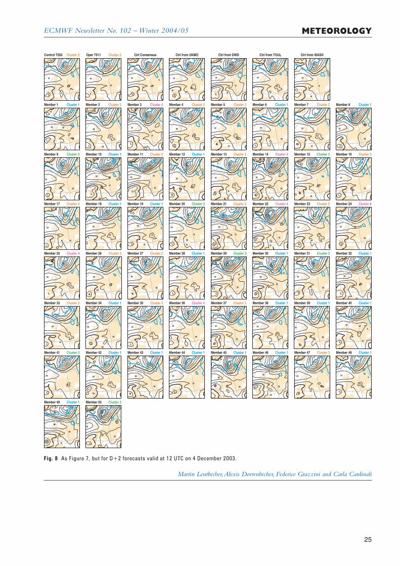
ECMWF Newsletter No. 102 – Winter 2004/05
25
METEOROLOGY
H
H
L
L
L
H
H
L
H
H
L
L
L
L
LH
H
L
L
L
LH
H
HL
L
H
H
H
L
H
H
H
LL
L
H H
H
L
L
H
H
H
H
H
L
L
H
H
H
H
L
L
H
H
L
L
H
H
H
H
H L
L
L
H
HH
H
L
L
H
H
H
L
L
L
H
H
H
H
L
L
L
H
H
H
H
L
L
L
HH
H
H
L
L
L
L H
H
H
H
LL
H
H
H
H
L
L
H
H
H
L
L
L
H
H
H
H
L
L
H
H
H
LL
L
L
H
HH
H
L
H
H
H
H
H
L
L
H
H
HL
L
H
H
H
L
L
L H
H
H
H
L
L
H
H
L
L
L H
H
H
H
L
L
H
H
H
L
L
L
H H
H
L
L
L
4
H
H
HL
L
H
H
H
L
L
L
H
HH
L
L
L
L H
H
L
H
H
H
HL
L
L
H
H
H
H
L
L
L
H
H
HH
L
L
L
H
H
L
L
H
H
H
H
L
L
LH
H
H
L
L
L
H
H
L
L
H
H
H
H
LL
H
H
L
L
1027H
H
LL
H
HH
H
L
L
L
H H
H
H
H
L
L
L
H
H
L
L
L
H
H
H
L
L
H
H
L
L
L
L
H
H
L
L
L
H
HH
H
L
H
H
H
L
L
L
L
H
H
L
L
H
H
L
L
L
H
H
HL
L
L
H
H
H
H
L
L
Control T255 Oper T511 Ctrl Consensus Ctrl from UKMO Ctrl from DWD Ctrl from TOUL Ctrl from WASH
Member 1 Member 2Cluster 1
Cluster 2 Cluster 2
Cluster 2 Member 3 Member 4Cluster 4 Cluster 2 Member 5 Member 6Cluster 2 Cluster 1 Member 7 Member 8Cluster 2 Cluster 1
Member 9 Member 10Cluster 3 Cluster 1 Member 11 Member 12Cluster 2 Cluster 1 Member 13 Member 14Cluster 2 Cluster 4 Member 15 Member 16Cluster 3 Cluster 2
Member 17 Member 18Cluster 2 Cluster 1 Member 19 Member 20Cluster 1 Cluster 3 Member 21 Member 22Cluster 2 Cluster 4 Member 23 Member 24Cluster 2 Cluster 4
Member 33 Member 34Cluster 2 Cluster 1 Member 35 Member 36Cluster 2 Cluster 4 Member 37 Member 38Cluster 2 Cluster 1 Member 39 Member 40Cluster 1 Cluster 1
Member 41 Member 42Cluster 3 Cluster 1
Member 49 Member 50Cluster 1 Cluster 3
Member 43 Member 44Cluster 1 Cluster 1 Member 45 Member 46Cluster 1 Cluster 1 Member 47 Member 48Cluster 2 Cluster 1
Member 25 Member 26Cluster 4 Cluster 2 Member 27 Member 28Cluster 2 Cluster 1 Member 29 Member 30Cluster 3 Cluster 1 Member 31 Member 32Cluster 3 Cluster 1
Fig. 8 As Figure 7, but for D+2 forecasts valid at 12 UTC on 4 December 2003.
Martin Leutbecher,Alexis Doerenbecher, Federico Grazzini and Carla Cardinali
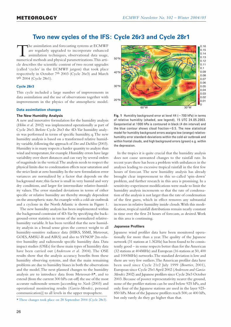
ECMWF Newsletter No. 102 – Winter 2004/05
26
METEOROLOGY
The assimilation and forecasting systems at ECMWFare regularly upgraded to incorporate enhancedassimilation techniques, observational data usage,
numerical methods and physical parametrizations.This arti-cle describes the scientific content of two recent upgrades(called ‘cycles’ in the ECMWF jargon) that took placerespectively in October 7th 2003 (Cycle 26r3) and March9th 2004 (Cycle 28r1).
Cycle 26r3
This cycle included a large number of improvements indata assimilation and the use of observations together withimprovements in the physics of the atmospheric model.
Data assimilation changes
The New Humidity AnalysisA new and innovative formulation for the humidity analysis(Hólm et al. 2002) was implemented operationally as part ofCycle 26r3. Before Cycle 26r3 the 4D-Var humidity analy-sis was performed in terms of specific humidity, q.The newhumidity analysis is based on a transformed relative humid-ity variable, following the approach of Dee and DaSilva (2003).Humidity is in many respects a harder quantity to analyze thanwind and temperature, for example.Humidity errors have largevariability over short distances and can vary by several ordersof magnitude in the vertical.The analysis needs to respect thephysical limits due to condensation effects near saturation andthe strict limit at zero humidity. In the new formulation errorvariances are normalized by a factor that depends on thebackground state; this factor is small in very humid and verydry conditions, and larger for intermediate relative-humid-ity values. The error standard deviations in terms of eitherspecific or relative humidity are thereby strongly dependenton the atmospheric state.An example with a cold-air outbreakand a cyclone in the North Atlantic is shown in Figure 1.
The new humidity analysis has been implemented withinthe background constraint of 4D-Var by specifying the back-ground-error statistics in terms of the normalized relative-humidity variable. It has been verified that the new humid-ity analysis in a broad sense gives the correct weight to allhumidity-sensitive radiance data (HIRS, SSMI, Meteosat,GOES,AMSU-B and AIRS) and also to SYNOP 2m-rela-tive humidity and radiosonde specific humidity data. Dataimpact studies (OSEs) for these main types of humidity datahave been carried out (Andersson et al. 2004). The OSEresults show that the analysis accuracy benefits from thesehumidity observing systems, and that the main remainingproblems are due to humidity biases in both the observationsand the model.The next planned changes to the humidityanalysis are to introduce data from Meteosat-8*, and toextend (from the current 300 hPa cut-off) the use of the mostaccurate radiosonde sensors [according to Nash (2003) andoperational monitoring results (Garcia-Mendez, personalcommunication)] to all levels in the upper troposphere.
In the tropics it is quite crucial that the humidity analysisdoes not cause unwanted changes to the rainfall rate. Inrecent years there has been a problem with unbalances in theanalyses leading to excessive tropical rainfall in the first fewhours of forecast. The new humidity analysis has alreadybrought clear improvement to this so-called ‘spin-down’problem, and further research in this area is promising. In asensitivity-experiment modifications were made to limit thehumidity analysis increments so that the rate of condensa-tion of the analysis is not larger than the rate of condensationof the first guess, which in effect removes any substantialincreases in relative humidity inside clouds.With this modi-fication, tropical rainfall distributions remain nearly constantin time over the first 24 hours of forecasts, as desired.Workin this area is continuing.
Japanese Profilers
Japanese wind profiler data have been monitored opera-tionally for more than a year. The quality of the Japanesenetwork (31 stations at 1.3GHz) has been found to be consis-tently good – in some respects better than for the American(32 stations at 404MHz) and European (16 stations at 50, 400and 1000MHz) networks.The standard deviation is low andthere are very few outliers.The American profiler data havebeen used since Cycle 21r2 July 1999 (Bouttier, 2001),European since Cycle 25r1 April 2002 (Andersson and Garcia-Mendez 2002) and Japanese profilers since Cycle 26r3 October2003. Because of poorer representativity nearer the ground,none of the profiler stations can be used below 925 hPa, andonly four of the Japanese stations are used in the layer 925-850 hPa.Most of the Japanese profilers reach 500,or 400 hPa,but only rarely do they go higher than that.
Two new cycles of the IFS: Cycle 26r3 and Cycle 28r1
H
HH
L
L
L
L
L
8
16
16
16
16
20°N
60°W 30°W
30°N
40°N
50°N
0
0.01
0.02
0.03
0.04
0.05
0.06
0.07
0.08
0.09
0.1
0.11
0.12
0.13
0.14
0.15
0.16
0.50.5
0.50.5
0.50.5
0.50.5
0.50.5
Fig. 1 Humidity background error at level 44 (~700 hPa) in termsof relative humidity (shaded, see legend), 15 UTC 24.05.2003.Geopotential at 1000 hPa is contoured in black (4 dm interval) andthe blue contour shows cloud fraction=0.5. The new statisticalmodel for humidity background errors assigns low (orange) relative-humidity error standard-deviations within the cold-air outbreak andwithin frontal clouds, and high background errors (green) e.g. withinthe depression.
* These changes took place on 28 September 2004 (Cycle 28r3).
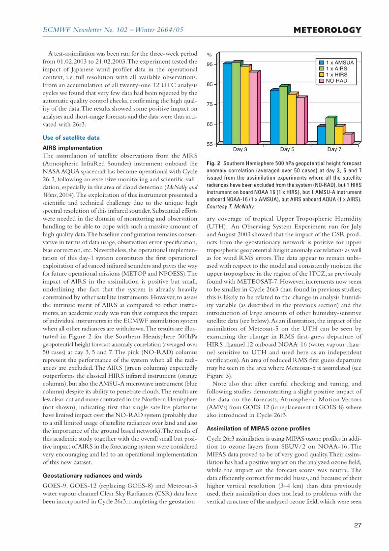
ECMWF Newsletter No. 102 – Winter 2004/05
27
METEOROLOGY
A test-assimilation was been run for the three-week periodfrom 01.02.2003 to 21.02.2003.The experiment tested theimpact of Japanese wind profiler data in the operationalcontext, i.e. full resolution with all available observations.From an accumulation of all twenty-one 12 UTC analysiscycles we found that very few data had been rejected by theautomatic quality control checks, confirming the high qual-ity of the data.The results showed some positive impact onanalyses and short-range forecasts and the data were thus acti-vated with 26r3.
Use of satellite data
AIRS implementationThe assimilation of satellite observations from the AIRS(Atmospheric InfraRed Sounder) instrument onboard theNASA AQUA spacecraft has become operational with Cycle26r3, following an extensive monitoring and scientific vali-dation, especially in the area of cloud detection (McNally andWatts, 2004).The exploitation of this instrument presented ascientific and technical challenge due to the unique highspectral resolution of this infrared sounder. Substantial effortswere needed in the domain of monitoring and observationhandling to be able to cope with such a massive amount ofhigh quality data.The baseline configuration remains conser-vative in terms of data usage, observation error specification,bias correction, etc.Nevertheless, the operational implemen-tation of this day-1 system constitutes the first operationalexploitation of advanced infrared sounders and paves the wayfor future operational missions (METOP and NPOESS).Theimpact of AIRS in the assimilation is positive but small,underlining the fact that the system is already heavilyconstrained by other satellite instruments. However, to assessthe intrinsic merit of AIRS as compared to other instru-ments, an academic study was run that compares the impactof individual instruments in the ECMWF assimilation systemwhen all other radiances are withdrawn.The results are illus-trated in Figure 2 for the Southern Hemisphere 500hPageopotential height forecast anomaly correlation (averaged over50 cases) at day 3, 5 and 7.The pink (NO-RAD) columnsrepresent the performance of the system when all the radi-ances are excluded.The AIRS (green columns) expectedlyoutperforms the classical HIRS infrared instrument (orangecolumns), but also the AMSU-A microwave instrument (bluecolumn) despite its ability to penetrate clouds.The results areless clear-cut and more contrasted in the Northern Hemisphere(not shown), indicating first that single satellite platformshave limited impact over the NO-RAD system (probably dueto a still limited usage of satellite radiances over land and alsothe importance of the ground based network).The results ofthis academic study together with the overall small but posi-tive impact of AIRS in the forecasting system were consideredvery encouraging and led to an operational implementationof this new dataset.
Geostationary radiances and winds
GOES-9, GOES-12 (replacing GOES-8) and Meteosat-5water vapour channel Clear Sky Radiances (CSR) data havebeen incorporated in Cycle 26r3, completing the geostation-
ary coverage of tropical Upper Tropospheric Humidity(UTH). An Observing System Experiment run for Julyand August 2003 showed that the impact of the CSR prod-ucts from the geostationary network is positive for uppertropospheric geopotential height anomaly correlations as wellas for wind RMS errors.The data appear to remain unbi-ased with respect to the model and consistently moisten theupper troposphere in the region of the ITCZ, as previouslyfound with METEOSAT-7. However, increments now seemto be smaller in Cycle 26r3 than found in previous studies;this is likely to be related to the change in analysis humid-ity variable (as described in the previous section) and theintroduction of large amounts of other humidity-sensitivesatellite data (see below).As an illustration, the impact of theassimilation of Meteosat-5 on the UTH can be seen byexamining the change in RMS first-guess departure ofHIRS channel 12 onboard NOAA-16 (water vapour chan-nel sensitive to UTH and used here as an independentverification).An area of reduced RMS first guess departuremay be seen in the area where Meteosat-5 is assimilated (seeFigure 3).
Note also that after careful checking and tuning, andfollowing studies demonstrating a slight positive impact ofthe data on the forecasts, Atmospheric Motion Vectors(AMVs) from GOES-12 (in replacement of GOES-8) wherealso introduced in Cycle 26r3.
Assimilation of MIPAS ozone profiles
Cycle 26r3 assimilation is using MIPAS ozone profiles in addi-tion to ozone layers from SBUV/2 on NOAA-16. TheMIPAS data proved to be of very good quality.Their assim-ilation has had a positive impact on the analyzed ozone field,while the impact on the forecast scores was neutral. Thedata efficiently correct for model biases, and because of theirhigher vertical resolution (3–4 km) than data previouslyused, their assimilation does not lead to problems with thevertical structure of the analyzed ozone field,which were seen
Day 355
65
75
85
95
%
Day 5 Day 7
1 x AMSUA1 x AIRS1 x HIRSNO-RAD
Fig. 2 Southern Hemisphere 500 hPa geopotential height forecastanomaly correlation (averaged over 50 cases) at day 3, 5 and 7issued from the assimilation experiments where all the satelliteradiances have been excluded from the system (NO-RAD), but 1 HIRSinstrument on board NOAA 16 (1 x HIRS), but 1 AMSU-A instrumentonboard NOAA-16 (1 x AMSUA), but AIRS onboard AQUA (1 x AIRS).Courtesy T. McNally.
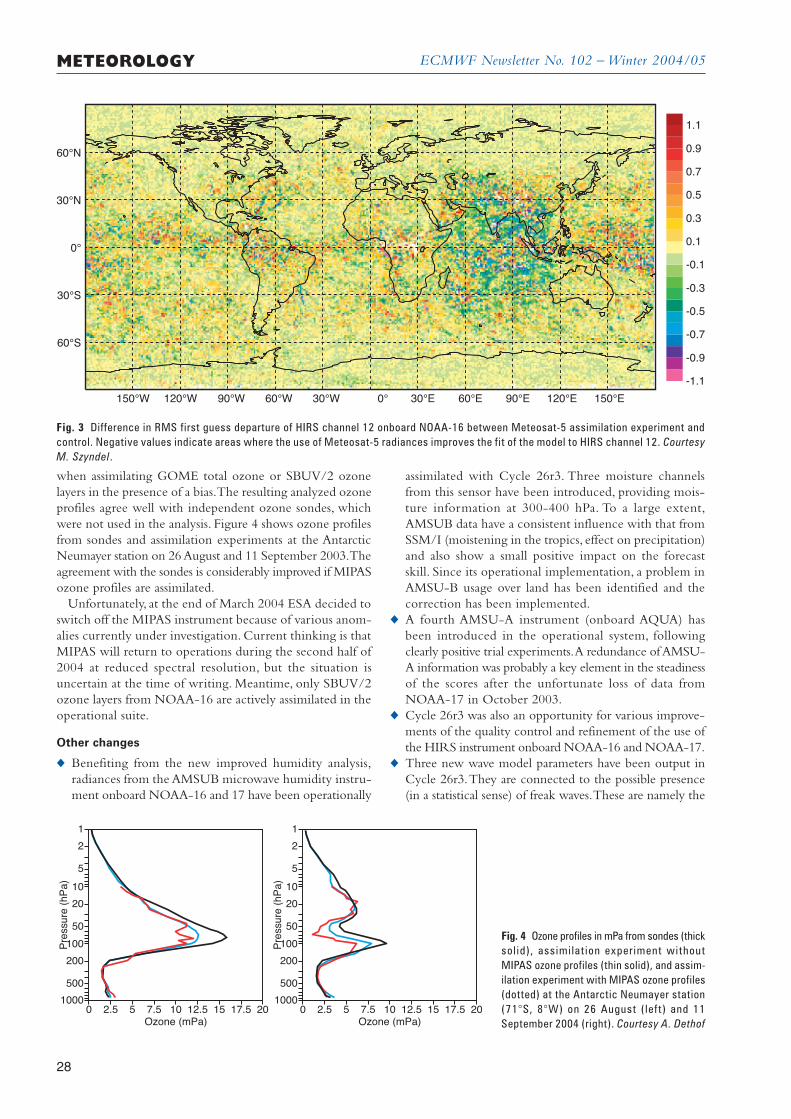
ECMWF Newsletter No. 102 – Winter 2004/05
28
METEOROLOGY
when assimilating GOME total ozone or SBUV/2 ozonelayers in the presence of a bias.The resulting analyzed ozoneprofiles agree well with independent ozone sondes, whichwere not used in the analysis. Figure 4 shows ozone profilesfrom sondes and assimilation experiments at the AntarcticNeumayer station on 26 August and 11 September 2003.Theagreement with the sondes is considerably improved if MIPASozone profiles are assimilated.
Unfortunately, at the end of March 2004 ESA decided toswitch off the MIPAS instrument because of various anom-alies currently under investigation. Current thinking is thatMIPAS will return to operations during the second half of2004 at reduced spectral resolution, but the situation isuncertain at the time of writing. Meantime, only SBUV/2ozone layers from NOAA-16 are actively assimilated in theoperational suite.
Other changes
u Benefiting from the new improved humidity analysis,radiances from the AMSUB microwave humidity instru-ment onboard NOAA-16 and 17 have been operationally
assimilated with Cycle 26r3. Three moisture channelsfrom this sensor have been introduced, providing mois-ture information at 300-400 hPa. To a large extent,AMSUB data have a consistent influence with that fromSSM/I (moistening in the tropics, effect on precipitation)and also show a small positive impact on the forecastskill. Since its operational implementation, a problem inAMSU-B usage over land has been identified and thecorrection has been implemented.
u A fourth AMSU-A instrument (onboard AQUA) hasbeen introduced in the operational system, followingclearly positive trial experiments.A redundance of AMSU-A information was probably a key element in the steadinessof the scores after the unfortunate loss of data fromNOAA-17 in October 2003.
u Cycle 26r3 was also an opportunity for various improve-ments of the quality control and refinement of the use ofthe HIRS instrument onboard NOAA-16 and NOAA-17.
u Three new wave model parameters have been output inCycle 26r3.They are connected to the possible presence(in a statistical sense) of freak waves.These are namely the
-1.1
-0.9
-0.7
-0.5
-0.3
-0.1
0.1
0.3
0.5
0.7
0.9
1.1
150°W 120°W 90°W 60°W 30°W 0° 30°E 60°E 90°E 120°E 150°E
60°S
30°S
0°
30°N
60°N
Fig. 3 Difference in RMS first guess departure of HIRS channel 12 onboard NOAA-16 between Meteosat-5 assimilation experiment andcontrol. Negative values indicate areas where the use of Meteosat-5 radiances improves the fit of the model to HIRS channel 12. CourtesyM. Szyndel.
1
2
5
10
20
50
100
200
500
0 2.5 5 7.5 10Ozone (mPa)
12.5 15 17.5 201000
Pre
ssure
(hP
a)
1
2
5
10
20
50
100
200
500
0 2.5 5 7.5 10Ozone (mPa)
12.5 15 17.5 201000
Pre
ssure
(hP
a)
Fig. 4 Ozone profiles in mPa from sondes (thicksol id), assimi lat ion experiment withoutMIPAS ozone profiles (thin solid), and assim-ilation experiment with MIPAS ozone profiles(dotted) at the Antarctic Neumayer station(71°S, 8°W) on 26 August ( left) and 11September 2004 (right). Courtesy A. Dethof
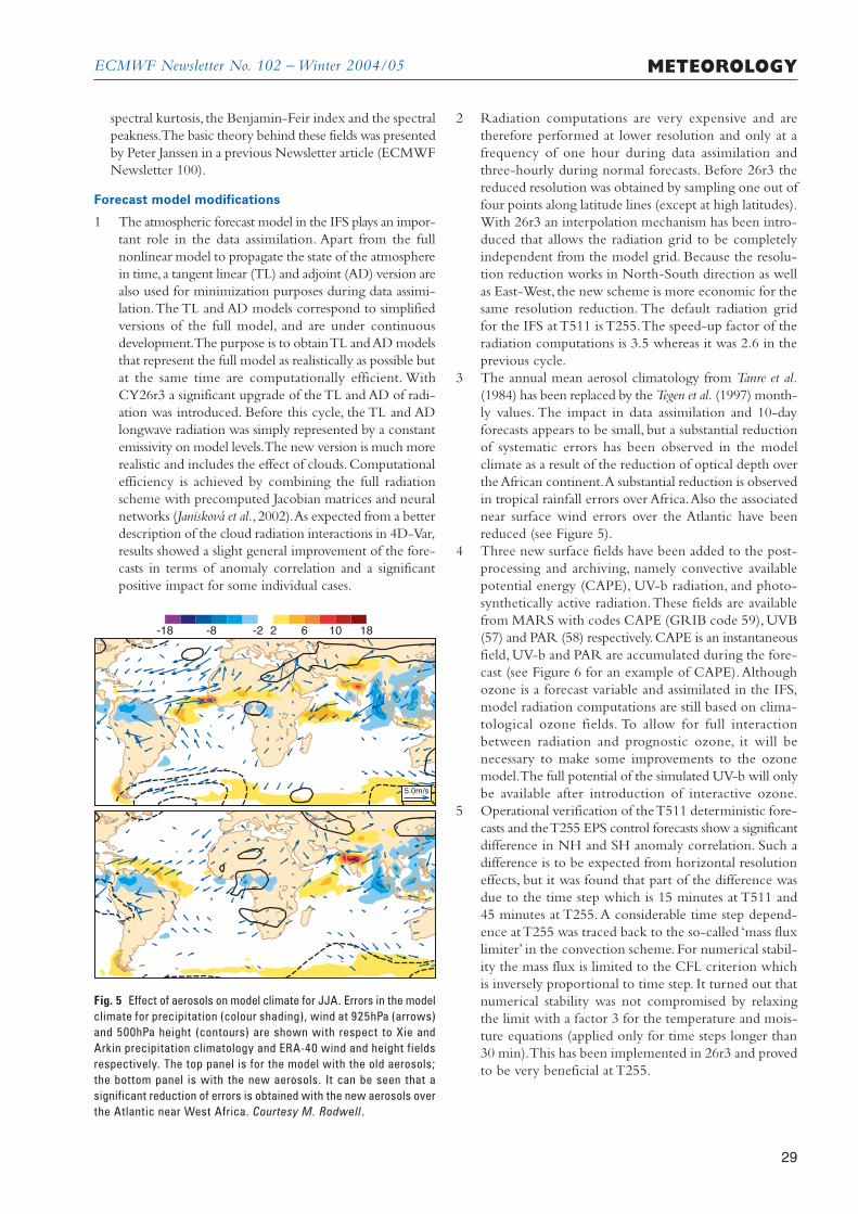
ECMWF Newsletter No. 102 – Winter 2004/05
29
METEOROLOGY
spectral kurtosis, the Benjamin-Feir index and the spectralpeakness.The basic theory behind these fields was presentedby Peter Janssen in a previous Newsletter article (ECMWFNewsletter 100).
Forecast model modifications
1 The atmospheric forecast model in the IFS plays an impor-tant role in the data assimilation. Apart from the fullnonlinear model to propagate the state of the atmospherein time,a tangent linear (TL) and adjoint (AD) version arealso used for minimization purposes during data assimi-lation.The TL and AD models correspond to simplifiedversions of the full model, and are under continuousdevelopment.The purpose is to obtain TL and AD modelsthat represent the full model as realistically as possible butat the same time are computationally efficient. WithCY26r3 a significant upgrade of the TL and AD of radi-ation was introduced. Before this cycle, the TL and ADlongwave radiation was simply represented by a constantemissivity on model levels.The new version is much morerealistic and includes the effect of clouds. Computationalefficiency is achieved by combining the full radiationscheme with precomputed Jacobian matrices and neuralnetworks (Janisková et al., 2002).As expected from a betterdescription of the cloud radiation interactions in 4D-Var,results showed a slight general improvement of the fore-casts in terms of anomaly correlation and a significantpositive impact for some individual cases.
2 Radiation computations are very expensive and aretherefore performed at lower resolution and only at afrequency of one hour during data assimilation andthree-hourly during normal forecasts. Before 26r3 thereduced resolution was obtained by sampling one out offour points along latitude lines (except at high latitudes).With 26r3 an interpolation mechanism has been intro-duced that allows the radiation grid to be completelyindependent from the model grid. Because the resolu-tion reduction works in North-South direction as wellas East-West, the new scheme is more economic for thesame resolution reduction. The default radiation gridfor the IFS at T511 is T255.The speed-up factor of theradiation computations is 3.5 whereas it was 2.6 in theprevious cycle.
3 The annual mean aerosol climatology from Tanre et al.(1984) has been replaced by the Tegen et al. (1997) month-ly values. The impact in data assimilation and 10-dayforecasts appears to be small, but a substantial reductionof systematic errors has been observed in the modelclimate as a result of the reduction of optical depth overthe African continent.A substantial reduction is observedin tropical rainfall errors over Africa.Also the associatednear surface wind errors over the Atlantic have beenreduced (see Figure 5).
4 Three new surface fields have been added to the post-processing and archiving, namely convective availablepotential energy (CAPE), UV-b radiation, and photo-synthetically active radiation.These fields are availablefrom MARS with codes CAPE (GRIB code 59), UVB(57) and PAR (58) respectively.CAPE is an instantaneousfield, UV-b and PAR are accumulated during the fore-cast (see Figure 6 for an example of CAPE).Althoughozone is a forecast variable and assimilated in the IFS,model radiation computations are still based on clima-tological ozone fields. To allow for full interactionbetween radiation and prognostic ozone, it will benecessary to make some improvements to the ozonemodel.The full potential of the simulated UV-b will onlybe available after introduction of interactive ozone.
5 Operational verification of the T511 deterministic fore-casts and the T255 EPS control forecasts show a significantdifference in NH and SH anomaly correlation. Such adifference is to be expected from horizontal resolutioneffects, but it was found that part of the difference wasdue to the time step which is 15 minutes at T511 and45 minutes at T255. A considerable time step depend-ence at T255 was traced back to the so-called ‘mass fluxlimiter’ in the convection scheme. For numerical stabil-ity the mass flux is limited to the CFL criterion whichis inversely proportional to time step. It turned out thatnumerical stability was not compromised by relaxingthe limit with a factor 3 for the temperature and mois-ture equations (applied only for time steps longer than30 min).This has been implemented in 26r3 and provedto be very beneficial at T255.
-18 -8 -2 2 6 10 18
5.0m/s
Fig. 5 Effect of aerosols on model climate for JJA. Errors in the modelclimate for precipitation (colour shading), wind at 925hPa (arrows)and 500hPa height (contours) are shown with respect to Xie andArkin precipitation climatology and ERA-40 wind and height fieldsrespectively. The top panel is for the model with the old aerosols;the bottom panel is with the new aerosols. It can be seen that asignificant reduction of errors is obtained with the new aerosols overthe Atlantic near West Africa. Courtesy M. Rodwell.
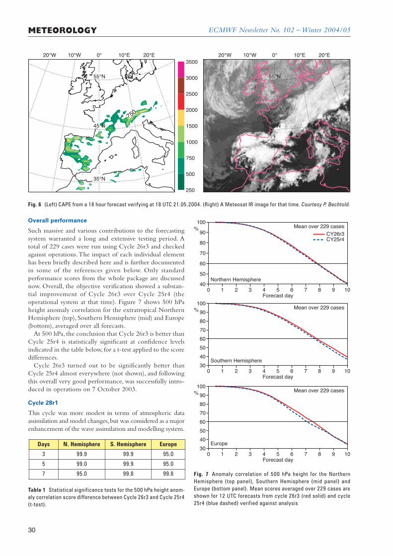
ECMWF Newsletter No. 102 – Winter 2004/05
30
METEOROLOGY
Overall performance
Such massive and various contributions to the forecastingsystem warranted a long and extensive testing period. Atotal of 229 cases were run using Cycle 26r3 and checkedagainst operations.The impact of each individual elementhas been briefly described here and is further documentedin some of the references given below. Only standardperformance scores from the whole package are discussednow. Overall, the objective verification showed a substan-tial improvement of Cycle 26r3 over Cycle 25r4 (theoperational system at that time). Figure 7 shows 500 hPaheight anomaly correlation for the extratropical NorthernHemisphere (top), Southern Hemisphere (mid) and Europe(bottom), averaged over all forecasts.
At 500 hPa, the conclusion that Cycle 26r3 is better thanCycle 25r4 is statistically significant at confidence levelsindicated in the table below, for a t-test applied to the scoredifferences.
Cycle 26r3 turned out to be significantly better thanCycle 25r4 almost everywhere (not shown), and followingthis overall very good performance, was successfully intro-duced in operations on 7 October 2003.
Cycle 28r1
This cycle was more modest in terms of atmospheric dataassimilation and model changes,but was considered as a majorenhancement of the wave assimilation and modelling system.
Days N. Hemisphere S. Hemisphere Europe
3 99.9 99.9 95.0
5 99.0 99.9 95.0
7 95.0 99.8 99.8
750
20°W 10°W 0° 10°E 20°E
250
500
750
1000
1500
2000
2500
3000
3500
45°N
55°N
35°N
20°W 10°W 0° 10°E 20°E
45°N
55°N
35°N
Fig. 6 (Left) CAPE from a 18 hour forecast verifying at 18 UTC 21.05.2004. (Right) A Meteosat IR image for that time. Courtesy P. Bechtold.
Table 1 Statistical significance tests for the 500 hPa height anom-aly correlation score difference between Cycle 26r3 and Cycle 25r4(t-test).
0 1 2 3 4 5 6 7 8 9 10Forecast day
40
50
60
70
80
90
100
%
0 1 2 3 4 5 6 7 8 9 10Forecast day
30
40
50
60
70
80
90
100
%
0 1 2 3 4 5 6 7 8 9 10Forecast day
30
40
50
60
70
80
90
100
%
Mean over 229 cases
Mean over 229 cases
Mean over 229 cases
CY26r3CY25r4
Northern Hemisphere
Southern Hemisphere
Europe
Fig. 7 Anomaly correlation of 500 hPa height for the NorthernHemisphere (top panel), Southern Hemisphere (mid panel) andEurope (bottom panel). Mean scores averaged over 229 cases areshown for 12 UTC forecasts from cycle 26r3 (red solid) and cycle25r4 (blue dashed) verified against analysis
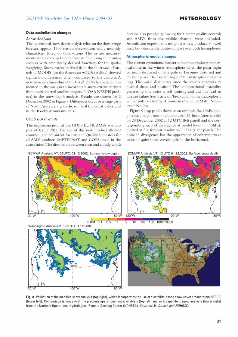
ECMWF Newsletter No. 102 – Winter 2004/05
became also possible (allowing for a better quality control)and AMVs from the visible channel were included.Assimilation experiments using these new products showedsmall but consistently positive impact over both hemispheres.
Atmospheric model changes
The current operational forecast sometimes produces numer-ical noise in the winter stratosphere when the polar nightvortex is displaced off the pole or becomes distorted andbreaks up, as is the case during sudden stratospheric warm-ings. The noise disappears once the vortex recovers itsnormal shape and position. The computational instabilitygenerating this noise is self-limiting and did not lead toforecast failure (see article on ‘breakdown of the stratosphericwinter polar vortex’ by A. Simmons et al. in ECMWF News-letter No 96).
Figure 9 (top panel) shows as an example the 10hPa geo-potential height from the operational 12-hour forecast validon 28 December 2002 at 12 UTC (left panel) and the cor-responding map of divergence at model level 11 (~5hPa),plotted at full forecast resolution TL511 (right panel).Thenoise in divergence has the appearance of coherent wavetrains of quite short wavelengths in the horizontal.
Data assimilation changes
Snow AnalysisThe operational snow depth analysis relies on the short-rangeforecast, approx. 1500 station observations and a monthlyclimatology based on observations. The in-situ measure-ments are used to update the forecast field using a Cressmananalysis with empirically derived functions for the spatialweighting. Snow extent derived from the shortwave chan-nels of MODIS (on the American AQUA satellite) showedsignificant differences when compared to the analysis. Anew two-step algorithm (Drusch et al. 2004) has been imple-mented in the analysis to incorporate snow extent derivedfrom multi-spectral satellite imagery (NOAA NESDIS prod-uct) in the snow depth analysis. Results are shown for 2December 2002 in Figure 8.Differences occur over large partsof North America, e.g. to the south of the Great Lakes, andin the Rocky Mountains area.
GOES BUFR winds
The implementation of the GOES BUFR AMVs was alsopart of Cycle 28r1. The use of this new product allowedcommon and consistent formats and Quality Indicators forall AMV products (METEOSAT and GOES) used in theassimilation.The distinction between clear and cloudy winds
31
METEOROLOGY
Washington Analysis VT: 22UTC 01.12.2002
40°N
50°N
120°W 100°W 80°W
40°N
50°N
120°W 100°W 80°W
ECMWF Analysis VT: 06UTC, 01.12.2002. Surface: snow depth
40°N
50°N
120°W 100°W 80°W
ECMWF Analysis VT: 12 UTC 01.12.2002. Surface: snow depth
0.001 0.1 0.5 1 5 10 50 100 1000 10000
Fig. 8 Validation of the modified snow analysis (top right), which incorporates the use of a satellite-based snow cover product from NESDIS(lower left). Comparison is made with the previous operational snow analysis (top left) and an independent snow analysis (lower right)from the National Operational Hydrological Remote Sensing Center (NOHRSC). Courtesy M. Drusch and NOHRSC.
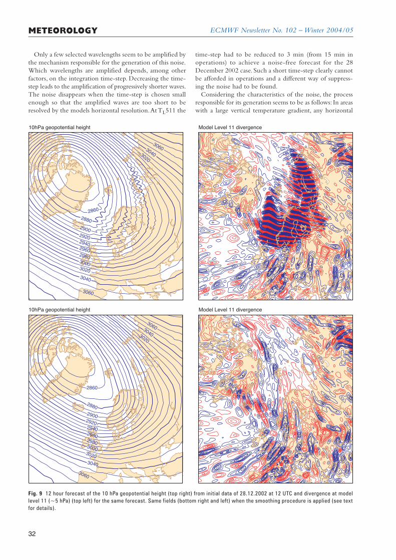
ECMWF Newsletter No. 102 – Winter 2004/05
Only a few selected wavelengths seem to be amplified bythe mechanism responsible for the generation of this noise.Which wavelengths are amplified depends, among otherfactors, on the integration time-step. Decreasing the time-step leads to the amplification of progressively shorter waves.The noise disappears when the time-step is chosen smallenough so that the amplified waves are too short to beresolved by the models horizontal resolution.At TL511 the
time-step had to be reduced to 3 min (from 15 min inoperations) to achieve a noise-free forecast for the 28December 2002 case. Such a short time-step clearly cannotbe afforded in operations and a different way of suppress-ing the noise had to be found.
Considering the characteristics of the noise, the processresponsible for its generation seems to be as follows: In areaswith a large vertical temperature gradient, any horizontal
32
METEOROLOGY
Model Level 11 divergence
2860
2880
2900292029402960298030003020
3020
3040
3040
3060
3060
10hPa geopotential height
Model Level 11 divergence
2860
2880
2900292029402960298030003020
3020
3040
3040
3060
3060
10hPa geopotential height
Fig. 9 12 hour forecast of the 10 hPa geopotential height (top right) from initial data of 28.12.2002 at 12 UTC and divergence at modellevel 11 (~5 hPa) (top left) for the same forecast. Same fields (bottom right and left) when the smoothing procedure is applied (see textfor details).
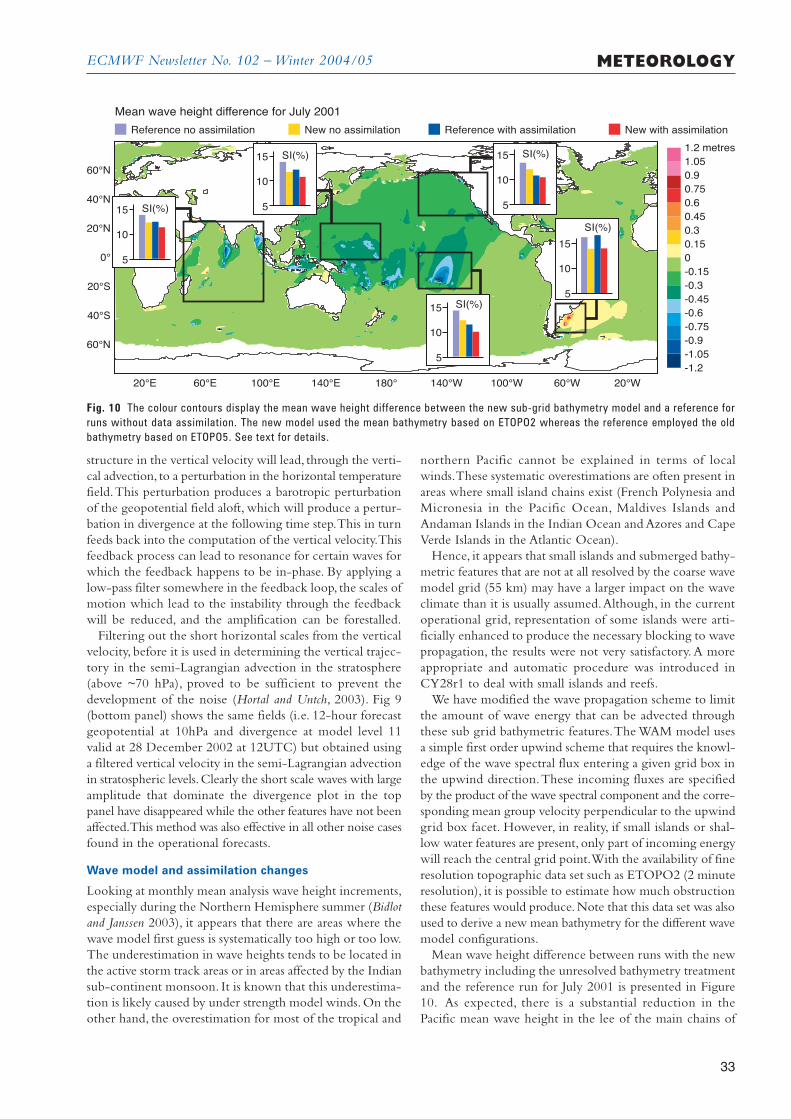
ECMWF Newsletter No. 102 – Winter 2004/05
structure in the vertical velocity will lead, through the verti-cal advection, to a perturbation in the horizontal temperaturefield.This perturbation produces a barotropic perturbationof the geopotential field aloft, which will produce a pertur-bation in divergence at the following time step.This in turnfeeds back into the computation of the vertical velocity.Thisfeedback process can lead to resonance for certain waves forwhich the feedback happens to be in-phase. By applying alow-pass filter somewhere in the feedback loop, the scales ofmotion which lead to the instability through the feedbackwill be reduced, and the amplification can be forestalled.
Filtering out the short horizontal scales from the verticalvelocity, before it is used in determining the vertical trajec-tory in the semi-Lagrangian advection in the stratosphere(above ~70 hPa), proved to be sufficient to prevent thedevelopment of the noise (Hortal and Untch, 2003). Fig 9(bottom panel) shows the same fields (i.e. 12-hour forecastgeopotential at 10hPa and divergence at model level 11valid at 28 December 2002 at 12UTC) but obtained usinga filtered vertical velocity in the semi-Lagrangian advectionin stratospheric levels.Clearly the short scale waves with largeamplitude that dominate the divergence plot in the toppanel have disappeared while the other features have not beenaffected.This method was also effective in all other noise casesfound in the operational forecasts.
Wave model and assimilation changes
Looking at monthly mean analysis wave height increments,especially during the Northern Hemisphere summer (Bidlotand Janssen 2003), it appears that there are areas where thewave model first guess is systematically too high or too low.The underestimation in wave heights tends to be located inthe active storm track areas or in areas affected by the Indiansub-continent monsoon. It is known that this underestima-tion is likely caused by under strength model winds. On theother hand, the overestimation for most of the tropical and
northern Pacific cannot be explained in terms of localwinds.These systematic overestimations are often present inareas where small island chains exist (French Polynesia andMicronesia in the Pacific Ocean, Maldives Islands andAndaman Islands in the Indian Ocean and Azores and CapeVerde Islands in the Atlantic Ocean).
Hence, it appears that small islands and submerged bathy-metric features that are not at all resolved by the coarse wavemodel grid (55 km) may have a larger impact on the waveclimate than it is usually assumed.Although, in the currentoperational grid, representation of some islands were arti-ficially enhanced to produce the necessary blocking to wavepropagation, the results were not very satisfactory. A moreappropriate and automatic procedure was introduced inCY28r1 to deal with small islands and reefs.
We have modified the wave propagation scheme to limitthe amount of wave energy that can be advected throughthese sub grid bathymetric features.The WAM model usesa simple first order upwind scheme that requires the knowl-edge of the wave spectral flux entering a given grid box inthe upwind direction.These incoming fluxes are specifiedby the product of the wave spectral component and the corre-sponding mean group velocity perpendicular to the upwindgrid box facet. However, in reality, if small islands or shal-low water features are present, only part of incoming energywill reach the central grid point.With the availability of fineresolution topographic data set such as ETOPO2 (2 minuteresolution), it is possible to estimate how much obstructionthese features would produce. Note that this data set was alsoused to derive a new mean bathymetry for the different wavemodel configurations.
Mean wave height difference between runs with the newbathymetry including the unresolved bathymetry treatmentand the reference run for July 2001 is presented in Figure10. As expected, there is a substantial reduction in thePacific mean wave height in the lee of the main chains of
33
METEOROLOGY
20°E 60°E 100°E 140°E 180° 140°W 100°W 60°W 20°W
60°N
40°N
20°N
0°
20°S
40°S
60°N
1.2 metres
1.05
0.9
0.75
0.6
0.45
0.3
0.15
0
-0.15
-0.3
-0.45
-0.6
-0.75
-0.9
-1.05
-1.2
5
10
15 SI(%) 5
10
15 SI(%)
5
10
15 SI(%)
5
10
15 SI(%)5
10
15
SI(%)
Reference no assimilation New no assimilation Reference with assimilation New with assimilation
Mean wave height difference for July 2001
Fig. 10 The colour contours display the mean wave height difference between the new sub-grid bathymetry model and a reference forruns without data assimilation. The new model used the mean bathymetry based on ETOPO2 whereas the reference employed the oldbathymetry based on ETOPO5. See text for details.
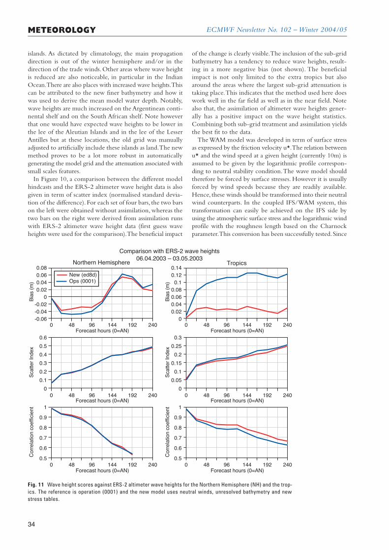
ECMWF Newsletter No. 102 – Winter 2004/05
islands. As dictated by climatology, the main propagationdirection is out of the winter hemisphere and/or in thedirection of the trade winds. Other areas where wave heightis reduced are also noticeable, in particular in the IndianOcean.There are also places with increased wave heights.Thiscan be attributed to the new finer bathymetry and how itwas used to derive the mean model water depth. Notably,wave heights are much increased on the Argentinean conti-nental shelf and on the South African shelf. Note howeverthat one would have expected wave heights to be lower inthe lee of the Aleutian Islands and in the lee of the LesserAntilles but at these locations, the old grid was manuallyadjusted to artificially include these islands as land.The newmethod proves to be a lot more robust in automaticallygenerating the model grid and the attenuation associated withsmall scales features.
In Figure 10, a comparison between the different modelhindcasts and the ERS-2 altimeter wave height data is alsogiven in term of scatter index (normalised standard devia-tion of the difference). For each set of four bars, the two barson the left were obtained without assimilation, whereas thetwo bars on the right were derived from assimilation runswith ERS-2 altimeter wave height data (first guess waveheights were used for the comparison).The beneficial impact
of the change is clearly visible.The inclusion of the sub-gridbathymetry has a tendency to reduce wave heights, result-ing in a more negative bias (not shown). The beneficialimpact is not only limited to the extra tropics but alsoaround the areas where the largest sub-grid attenuation istaking place.This indicates that the method used here doeswork well in the far field as well as in the near field. Notealso that, the assimilation of altimeter wave heights gener-ally has a positive impact on the wave height statistics.Combining both sub-grid treatment and assimilation yieldsthe best fit to the data.
The WAM model was developed in term of surface stressas expressed by the friction velocity u*.The relation betweenu* and the wind speed at a given height (currently 10m) isassumed to be given by the logarithmic profile correspon-ding to neutral stability condition.The wave model shouldtherefore be forced by surface stresses. However it is usuallyforced by wind speeds because they are readily available.Hence, these winds should be transformed into their neutralwind counterparts. In the coupled IFS/WAM system, thistransformation can easily be achieved on the IFS side byusing the atmospheric surface stress and the logarithmic windprofile with the roughness length based on the Charnockparameter.This conversion has been successfully tested. Since
34
METEOROLOGY
0.08
0.06
0.04
0.02
0
-0.02
-0.04
-0.06
0.6
0.5
0.4
0.3
0.2
0.1
0
1
0.9
0.8
0.7
0.6
0.5
0 48 96 144 192 240
0 48 96 144 192 240
0 48 96 144 192 240
0.14
0.12
0.1
0.08
0.06
0.04
0.02
0
0.3
0.25
0.2
0.15
0.1
0.05
0
1
0.9
0.8
0.7
0.6
0.5
0 48 96 144 192 240
0 48 96 144 192 240
0 48 96 144 192 240
Ops (0001)
Northern Hemisphere Tropics
Corr
ela
tion c
oeffic
ient
Scatter
Index
Bia
s (
m)
Corr
ela
tion c
oeffic
ient
Scatter
Index
Bia
s (
m)
Forecast hours (0=AN) Forecast hours (0=AN)
Forecast hours (0=AN) Forecast hours (0=AN)
Forecast hours (0=AN) Forecast hours (0=AN)
New (ed8d)
06.04.2003 – 03.05.2003
Comparison with ERS-2 wave heights
Fig. 11 Wave height scores against ERS-2 altimeter wave heights for the Northern Hemisphere (NH) and the trop-ics. The reference is operation (0001) and the new model uses neutral winds, unresolved bathymetry and newstress tables.
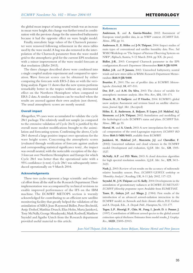
ECMWF Newsletter No. 102 – Winter 2004/05
the global mean impact of using neutral winds was an increasein mean wave height, this change was further tested in combi-nation with the previous change for the unresolved bathymetrybecause it had the opposite effect on wave height model.
Finally, unrealistic large values of the Charnock parame-ter were removed following refinement in the stress tablesused by the wave model.A bug was also removed in the inter-polation of the Charnock parameter from the wave modelgrid to the atmospheric grid for the current EPS resolutionwith a minor improvement of the wave model forecasts atthat resolution (Bidlot 2003).
The three changes described above were combined intoa single coupled analysis experiment and compared to oper-ation. Wave forecast scores can be obtained by eithercomparing the forecasts with ERS-2 data or with the veri-fying analysis. Figure 11 shows that the new system performsremarkably better in the tropics without any detrimentaleffect on the Northern Hemisphere when compared toERS-2 data.A similar conclusion can be reached when theresults are assessed against their own analysis (not shown).The usual atmospheric scores are mostly neutral.
Overall impact
Altogether, 99 cases were accumulated to validate the cycle28r1 package.The relatively small test sample (as comparedto the extensive validation of Cycle 26r3) is justified by theoverall more modest modifications brought to the assimi-lation and forecasting system. Confirming the above, Cycle28r1 showed a large positive impact over operations for thewave height scores. Concerning the atmospheric scores(evaluated through verification of forecasts against analysisand corresponding statistical significance tests) , the impactwas overall neutral,with the noticeable exception of the day-3 forecast over Northern Hemisphere and Europe for whichCycle 28r1 was better than the operational suite with a95% confidence (t-test). Cycle 28r1 was subsequently intro-duced operationally on 9 March 2004.
Acknowledgements
These two cycles represent a large scientific and techni-cal effort from all the staff in the Research Department.Theirimplementation was accompanied by technical revisions toenable improved performance of the IFS on the IBMmachine. The ECMWF METOPS section is warmlyacknowledged for contributing to an efficient new satellitemonitoring facility that greatly helped the validation of theassimilation of AIRS. Jean-Raymond Bidlot, Peter Bechtold,Antje Dethof,Matthias Drusch,Elias Holm,Marta Janisková,Tony McNally,George Mozdzynski,Mark Rodwell,MatthewSzyndel and Agathe Untch from the Research departmentprovided useful material to this article.
References
Andersson, E. and A. Garcia-Mendez, 2002: Assessment ofEuropean wind profiler data, in an NWP context. ECMWF Tech.Memo., 372, pp 14.
Andersson, E., E. Hólm and J-N.Thépaut, 2004: Impact studies ofmain types of conventional and satellite humidity data. Proc. 3rdWMO Workshop on ‘The Impact of Various Observing Systems onNWP’,Alpbach,Austria, 9-12 March 2004. pp XX. (In press).
Bidlot, J-R., 2003: Corrupted Charnock parameter in the EPSconfiguration.Research Department Memorandum R60.9/JB/0399.
Bidlot, J-R. and P. Janssen, 2003: Unresolved bathymetry, neutralwinds and new stress tables in WAM. Research Department Memo-randum R60.9/JB/0400.
Bouttier, F., 2001: The use of profiler data at ECMWF. Meteoro-logische Zeitschrift, 10, 497-510.
Dee, D.P., and A.M. Da Silva, 2003: The choice of variable foratmospheric moisture analysis. Mon.Wea. Rev., 131, 155-171.
Drusch, M., D. Vasiljevic and P. Viterbo, 2004: ECMWF’s globalsnow analysis: Assessment and revision based on satellite observa-tions. Journal Appl. Met. (Accepted)
Hólm, E., E. Andersson, A. Beljaars, P. Lopez, J-F. Mahfouf, A.J.Simmons and J-N. Thépaut, 2002: Assimilation and modelling ofthe hydrological cycle: ECMWF’s status and plans. ECMWF Tech.Memo., 383, pp 55.
Hortal, M. and A. Untch, 2003:A new interpolation for the verti-cal computation of the semi-Lagrangian trajectory. ECMWF RDMemo R60.5/MH/0415, available from ECMWF.
Janisková, M., Mahfouf, J-F., Morcrette, J-J. and Chevallier, F.(2002): Linearized radiation and cloud schemes in the ECMWFmodel: Development and evaluation, Q.J.R. Met. Soc., 128, 1505-1527.
McNally, A.P. and P.D. Watts, 2003: A cloud detection algorithmfor high spectral resolution sounders. Q.J.R. Met. Soc., 129, 3411-3423.
Nash, J., 2003: Review of test results on the accuracy of radiosonderelative humidity sensors. Proc. ECMWF/GEWEX workshop on‘Humidity Analysis’, Reading, UK, 8-11 July 2002, 117-123.
Szyndel, M., J-N.Thépaut and G. Kelly, 2004: Developments in theassimilation of geostationary radiances at ECMWF. EUMETSAT/ECMWF fellowship programme report.Available from EUMETSAT.
Tanre, D., Geleyn, J-F. and Slingo, J. (1984): First results of theintroduction of an advanced aerosol-radiation interaction in theECMWF model, in:Aerosols and their climate effects, H.E. Gerberand A. Deepak, Eds., A. Deepak Publ., Hampton,Va, 133-177.
Tegen, L.P., Hoorigl, P., Chin, M., Fung, I., Jacob, D. & Penner, J.(1997):Contribution of different aerosol species to the global aerosolextinction optical thickness: Estimates from model results, J. Geophys.Res., 102D, 23895-23915.
35
METEOROLOGY
Jean-Noël Thépaut, Erik Andersson,Anton Beljaars, Mariano Hortal and Peter Janssen
ECMWF Newsletter No. 102 – Winter 2004/05
The following is John Hennessy’s personal account of theearly days of computing at ECMWF, and of the diffi-culties in successfully producing the first operationalmedium-range forecast 25 years ago.
Text of message received from Dr. Lingelbach, Director of DeutscherWetterdienst.
36
COMPUTING
25 years since the first operational forecast
Subject: The issue of ECMWF’s firstoperational forecast
To: All members of staffDate: 2 August 1979From: J. Labrousse
Last night marked an important milestone in thedevelopment of the Centre’s work and activity.Despite a number of ‘technical hitches’, a medi-um-range operational forecast based on data of12Z, 1 August was completed, and the resultswere available in real-time to some at least ofour Member States. Products in chart form (1000and 500 mb fields for days 0 to 7) were trans-mitted via facsimile to the MeteorologicalOffice at Bracknell, who then relayed them toFrance and Germany. Copies of the same chartshave also been mailed to the other MemberStates. Attempts were also made to send theproducts in grid-point form over the low-speedtelecommunications link to Spain.
The Centre has received acknowledgement of andcongratulations on its efforts from both Germanyand France by telex; a translation of these mes-sages is attached.
I know that many in recent months have been work-ing very long hours to ensure that our long-planned goal of beginning operational activityin the middle of 1979 was achieved, and I wouldtake this opportunity to express my apprecia-tion to all staff who have contributed towardsthe production of the operational forecastingsystem. This is a major step forward and willbe welcomed enthusiastically by our MemberStates. There remain the major objectives ofimproving the meteorological quality of ourproducts and our operational reliability, sothat Member States will learn to trust and useour forecasts in the manner anticipated when theCentre was established.
Memo issued by the Head of Operations
Today Deutscher Wetterdienst received the firstproducts from the Centre, to be used as guid-ance in medium-range forecasting for the public.Being fully aware of all the problems the Centrehas had to overcome before this goal wasreached, Deutscher Wetterdienst congratulatesthe Director and all staff of the Centre, andwishes all success for the work to come; it willbe of benefit to all in Europe who are inter-ested in the weather.
We thank you for the reception of the first setof forecast charts produced by the Centre, andwe express our warm congratulations to you forthe work accomplished.
Text of message received from M. Gosset (for M. Mittner, Directorof Meteorologie Nationale)
Jean Labrousse, then Head of Operations, sent this memo-randum to all staff after completion of the Centre’s firstoperational forecast just over 25 years ago, and messages
of appreciation were received from Germany and France– at that time, of course, email was not available.The memo-randum itself looks a bit dated today: the use of SI Units hadnot become standard at ECMWF (mb instead of hPa), Zulutime was still in use (12Z) instead of Universal TimeCoordinated (UTC), and there is reference to ‘telex’(teleprinter exchange), a now obsolete communicationmethod.
The night of 1-2 August 1979 was certainly historic. I wasdelighted to be part of it and stayed at ECMWF overnightto be on hand to help with any problems that might arise withthe operational suite, particularly with the dissemination;wehad never had the opportunity for an end-to-end test witha Member State.The way in which an on-call system mightbe implemented was far from resolved.All went well to startwith. The taxi with the observational data in ‘raw’ GTSformat (character codes of the World MeteorologicalOrganization as transmitted on the Global TelecommunicationSystem) on magnetic tape arrived on time from the UnitedKingdom Meteorological Office in Bracknell, the preprocess-ing ran normally and so did the analysis cycles.Problems startedwith the forecast-model run; it got slower and slower. I hadvisions of it taking 12 days, which was as long as it took onthe CDC 6600 (ECMWF’s earlier model-developmentcomputer). However, the Systems Section had upgraded theCRAY operating system to level COS 1.3 on 1 August andhad informed me of this that afternoon.This was obviouslythe prime suspect for the problems.At my request the shiftleader took a memory dump, dropped the operating systemand reloaded the previous version.We restarted the suite, andthe rest is history. Initially, although the analysis cycles wererun over weekends, forecasts were run only from Monday toFriday. Daily running of the forecast did not begin until 1August 1980. The forecast run-time then was about fivehours.This is a far cry from the 47 minutes 30 seconds forthe forecast run for 14 May 1999,which is I believe the fastestever operational run of the forecast, achieved because we weretrying to make up for delays; we ran the forecast on 48Processing Elements on the Fujitsu VPP5000.
Prior to this, some trial medium-range forecasts had beencarried out on a semi-operational basis, using one-day-olddata.The first phase of EMOS (ECMWF’s MeteorologicalOperational System) had not yet been completed; this meantconsiderable manual intervention in running jobs to producethe forecasts.A series of these forecasts was prepared for the
ECMWF Newsletter No. 102 – Winter 2004/05
37
COMPUTING
official opening of ECMWF on 15 June 1979, and chartsdisplayed.These trial forecasts ‘showed useful skill from a fore-caster’s point of view’.
The years preceding this first operational run were verybusy in designing and implementing system and applicationutilities. ECMWF staff were in temporary office accommo-dation in Bracknell until the end of 1978, first in FitzwilliamHouse and John Scott House, which housed the CDC 6600computer, and later also in Brandon House.As well as hous-ing the computer, John Scott House was the venue for theCentre’s social gatherings. Staff had to push back the furni-ture and cardpunch machines to make room for the guests,and then restore everything before leaving at the end of theevening. Despite having three separate buildings, ECMWFdid not (unlike now) provide umbrellas for staff movingbetween buildings, but they did provide heavy-duty plasticbags, complete with the ECMWF name and logo, so thatprecious line-printer output and plots did not get wet.
ECMWF’s first Invitation to Tender, ITT(76)1, was issuedin mid-July 1976 for ‘the acquisition and installation of apowerful computer system’.The ITT makes very interest-ing reading nowadays.The volume of observational data tobe handled could be as high as 4 megabytes a day, the ten-day forecast was to be run in 10 hours and the volume ofdata (observations, analyses and forecast) to be archived wasestimated at 32 megabytes per day.Among the test programsto be executed by computer vendors were tests for cardreader, card punch and line printer.As a result of this ITT,the CRAY-1 and CDC Cyber 175 were selected, but notelecommunication system. The CRAY-1 was the onlymachine capable of running the forecast model in therequired time, but was not designed for stand-alone opera-tion, and so the Cyber 175 front-end kept all the permanentfiles and did the general housekeeping.
A separate ITT was issued in July 1977 for the telecom-munication system and a graphical display system. Atemporary installation of a limited configuration of theCRAY and Cyber systems was made at Rutherford Labora-tory (some 50 kilometres away)-the CRAY-1 in November1977 and the Cyber 175 in January 1978-with the machinesbeing run by the Centre’s operators. Remote Job Entryterminals in Fitzwilliam House and John Scott House wereconnected to the Cyber 175 and it was possible to submitjobs to both the CRAY-1 and the Cyber.The line printerin Fitzwilliam House was notorious for building up a largecharge of static electricity and it was quite common forusers to touch it with a coin to minimize the shock beforeattempting to remove the paper. As the link between theCRAY-1 and Cyber systems was not developed at this time,CRAY jobs submitted to the Cyber were staged to magnetictape.At intervals these jobs were manually transferred to theCRAY-1 via the tape unit on the CRAY operator station.A regular courier service also ran between Rutherford andBracknell to take jobs with large numbers of cards and bringback large amounts of printed output and plots. It was a reliefwhen the Cyber was moved to Shinfield and a new CRAY-1 was delivered there also, with a fully linked system beingput together towards the end of 1978. On 12 November the
operators working at Rutherford came to Shinfield and, asmany had only spoken to each other on the telephone andhad not met before, many people recognised each otheronly when they spoke.
The telecommunication system finally arrived in early1979. It was known as the Network Front End Processor(NFEP). Software was developed by Service in Informaticsand Analysis and the hardware was a Regnecentralen RC 8000computer.The NFEP interfaced to the Cyber 175 by emulat-ing a CDC Remote Job Entry terminal. For lines to MemberStates the communication protocols were based on the (thennew) CCITT Recommendation X25 and the IFIP proposal.Following installation there were further delays in doing theprovisional acceptance tests, as there were problems in themodules in medium-speed line connections.There were alsodelays in the provision of the actual circuits themselves.Thecomplete computer system then consisted of three differentmachines with three different operating systems, three differ-ent word lengths, three different byte lengths and two differentcharacter sets, all communicating with each other in a numberof different ways.
While all this was going on, work was also in progress onthe various components of EMOS-ECMWF’s Meteorolog-ical Operational System.The cornerstone of EMOS was thedesign and development of the Supervisor, known now asSMS-Supervisor Monitor Scheduler.Today’s SMS is a far cryfrom the original in its implementation, but the fundamen-tal principles have not changed, with families, tasks, eventsand messages all defined in the original SMS. SMS ran at asystem control point on the Cyber 175 and this enabled itto communicate with other suite (user) jobs. Events andmessages were communicated between the CRAY-1 andCyber by means of file transfers. Control of SMS was by theControl Display Program (CDP), a command-line interfaceto a teletype terminal. Only the operational suite wascontrolled by SMS,whereas nowadays SMS is used to controland run research experiments as well. SMS has been devel-oped from a Teletype, a line-mode system running one suiteon two machines, to an X-based system capable of control-ling multiple suites running on many machines.
As you will have gathered, the data acquisition systeminitially consisted of magnetic tapes delivered by taxi fromBracknell.The original plan was that ECMWF would usedecoded and quality-controlled observational data from upto three national meteorological centres, the data to betransmitted in a compact form on 4800 bps lines. Eachnational centre would send two thirds of the data on the GTS,so that ECMWF would receive two copies of all observa-tions. No decoding or quality-control programs would beneeded at ECMWF and this would avoid ‘duplication ofeffort’. Later this plan was amended, and the input obser-vational data were designated to be received from Bracknelland Offenbach in raw GTS format. Early 1980 saw the dataarrive in near real-time over a 2400 bps line from Bracknell,and later in the year from Offenbach as well. Files of obser-vations contained up to 250 bulletins; less than 250 occurredwhen 20 minutes had elapsed since the previous transmis-sion. On the NFEP, a batch job was prepared for the Cyber
ECMWF Newsletter No. 102 – Winter 2004/05
38
COMPUTING
with the observation file attached as input. On the Cyber,this job added the new bulletins to those already received-I say add, but initially this was not possible.The existing fileof bulletins had to be read and written to a new file, and itwas to this new file that the new data were then written.All observations at this time were in WMO character codes.As the volume of satellite data increased, compressed binarycodes became essential, but the GTS used character-orientedprotocols.A method was devised to transmit binary data overthe line from Washington.The six least significant bits of each8-bit character were used to transmit a 6-bit segment ofbinary data in a series of pseudo-ASCII characters. Thisstarted in 1984 and was used for many years until replacedby BUFR-coded data.
The preprocessing system decoded and quality controlledthe observations.These were interesting decoding programsbased on programs from the French National MeteorologicalService.The incoming observations were in ASCII (CCITTAlphabet No.5),but the Cyber had its own Display Code char-acters in six-bit bytes and so a lot of bit manipulation wasnecessary, the ASCII characters being stored in 12 bits (2bytes) on the Cyber. Most of the code was in assemblerlanguage but some was in Fortran 66, a language that had nocharacter type.This came only with Fortran 77 and the secondgeneration of decoding programs was written entirely inFortran 77, the first programs in the Centre in that language.The quality-control programs were adapted from those of theSwedish Meteorological and Hydrological Institute.A rudi-mentary ‘reports data base’ held the decoded andquality-controlled observations in a compact format, and fromthis database extractions were made for the analysis cycles.
Post-processing of the forecast model output generateddissemination products for the Member States. At that timethere was not the flexibility for specifying required prod-ucts that there is today. ECMWF had a fixed catalogue ofproducts, with fixed areas and resolutions. Initially onlyproducts up to seven days were disseminated.The format ofproducts was either the WMO GRID code or a compactbit-oriented grid code designed at ECMWF-no GRIB orBUFR machine-independent formats were available in thosedays.This ECMWF bit code continued for many years, andit was not until just before operations were switched to theFujitsu VPP700 in 1996 that the last dissemination productsin this code were issued. Files of analysis and forecast datawere sent to the NFEP for onward transmission to theMember States. The NFEP had to distinguish betweenbatch-job outputs and dissemination files.All disseminationfiles had unique names involving date/time, but all startedwith NBO. The NFEP software looked at file names andwhen a file with a name starting with NBO (Not BatchOutput) was encountered the first one or two records of thefile was read to ascertain where to send it and what the trans-mission filename was. Country addresses were simply asingle letter. A batch job, on punch cards, provided therepeat dissemination facility, with the operators having topunch two cards, one with country address letter and theother with the product catalogue numbers. An interestingevent occurred in September 1991 when the Americans
received forecasts from ECMWF for 2091. GRIB Edition1, with century of data included in the headers, was used forthe first time and the trans-Atlantic software interpretedcentury as the first two digits of the year!
An archive system was developed to store the operationaldata, both observations and fields, and to make it availableto general users.The data were stored on magnetic tapes onthe Cyber in a compressed format. A general-purposeretrieval procedure called GETDATA was provided to accessthe data on the Cyber.The early archives had a number ofgaps;we discovered that one of the programs storing the dataoccasionally ran into difficulty. Unfortunately, when it didit printed a message saying that the archiving had notcompleted fully and then issued a stop command instead ofan abort.Consequently nobody was aware of the failure whenit occurred.
As GETDATA began to show its age, a data-handlingproject was set up in 1982 and this produced MARS (Meteo-rological Archival and Retrieval System) based on CFS(now HPSS). This was essentially ‘client/server architec-ture’ before the name had been invented-indeed client/serverarchitectures did not appear in any great numbers until thelate 1980’s.We are all familiar today with ‘predictive-texting’for mobile telephones, but from day-1 the MARS languagealso had such predictive ability. Not everybody found thetransition to MARS a smooth one. One Member State userwrote “The phrase ‘user-friendly’ was not uppermost in mymind as I read the MARS User Guide (perhaps it is friendlyfor Martians)”.The author has wisely remained anonymous.– “The MARS system, as it exists now, is a giant step back-wards from GETDATA (which is far from perfect anyway)”.I admit to being the author.
It was a totally different working environment in the earlyyears. All documentation had to be handwritten (with hand-drawn diagrams) before being given to the secretaries fortyping.There were no desktop terminals or word processors.All programs were written in FORTRAN or assemblerlanguage. FORTRAN had a fixed format, a maximum of sixcharacters for variable names and no lower-case letters wereallowed.The program code had to be hand written on specialforms before putting it into an input tray at ComputerReception for punching onto cards. Inevitably there werealways errors in the punch cards due to poor handwriting andnot sticking to the conventions for Z and 7 and letter O andzero. It was quite normal to have several attempts at runningjobs before all punching errors were eliminated.
There was a very significant improvement in productiv-ity in programming when the ‘alphanumeric VDUs ‘ becamegenerally available.The introduction of the VDUs was grad-ual, and at the start of 1979 only 12 were in use with one‘graphical VDU’ supported.Using VDUs, some EMOS docu-mentation was produced by typing the text as comments ina FORTRAN program, doing a compilation and listingand trimming the resulting line-printer output which hada page-width of 132 characters.
Twenty-five years is a long time, especially in computingand related areas. Today, ECMWF’s supercomputers areroughly equivalent to 20,000 CRAY-1 systems. Changes
ECMWF Newsletter No. 102 – Winter 2004/05
39
COMPUTING / GENERAL
elsewhere have been equally dramatic.Telecommunications(with modems the size of suitcases) have come from one 50-baud line to the Regional Meteorological Data Network(RMDCN) combining ECMWF’s network with that ofWMO in Europe with also a very fast connection to theINTERNET. The volume of observational data hasincreased enormously, largely due to more and more satel-lite data, and now stands at about 2 gigabytes per day. Myrecollection is that on the first night we disseminated 27 prod-ucts. Now the volume and number of products disseminatedto Member States, the GTS and others via the INTERNET
stands at about 33 gigabytes and more than 2 million indi-vidual products. Graphical output was from one electrostaticplotter, now there are colour three-dimensional plots andmovies, all available on the office desktops as well as on hardcopy and the World Wide Web. Printing has also been revo-lutionized from a simple line printer (upper-case lettersonly) to colour, double-sided printing, with the ability toinclude graphics as well as text.There have been staggeringchanges in 25 years.Will the next 25 years bring as manychanges as have occurred since the pioneering days?
John Hennessy
Chaired by Anton Eliassen, the ECMWF Councilheld its 61st session in Reading on 13–14 December2004.The Council approved a 2% increase in the
Budget 2005 giving the Director flexibility to implementit. Other main results of this session were:
Amendments to the ECMWF Convention
The Council unanimously adopted recommendations of thePolicy Advisory Committee for amending the Conventionwith regard to the issue of languages at the Centre. Thisproposal does not alter the amendments to the Conventionalready adopted at Council’s 60th session in June 2004.
To formally adopt the Amending Protocol, Council willconvene an extra-ordinary session in April 2005.Thereafter,the official ratification process in the ECMWF MemberStates will start.
Co-operation Agreements
The Director was authorised by Council to conclude a Co-operation Agreement with the Republic of Lithuania and tosign Agreements with the European Space Agency (ESA) andthe Convention on Long-Range Transboundary Air Pollution(CLRTAP).
Regional Meteorological Data Communications Network
The Council agreed on the extension of the RMDCNcontract with Equant to March 2009. Amendments to thecontract will allow for a migration from Frame Relay toMulti Protocol Label Switching as well as a doubling of theaccess capacity for current RMDCN members.A new stan-dard connection of 768 kbps (at present 384 kbps) will beprovided to each ECMWF Member State.
Computing
The Director was authorised to extend the current contractwith IBM to cover supply of an enhanced High PerformanceComputing Facility until March 2009.This will result in theinstallation of a Phase 4 of the IBM system in Spring 2006with an aggregated sustained performance of 4.5 teraflops.
Four-Year Programme
The Council unanimously adopted the four-year programmeof activities. Its main goals are:u continue to extend the skill of both deterministic and
probabilistic medium-range forecasts at the rate of oneday per decade;
u extend the range of reliable forecasts of severe weatherover land and sea towards day 4 and day 5;
u develop a unified Ensemble Prediction System merging themedium-range EPS and the monthly forecasting system;
u continue the development of a multi-model seasonal/long-range prediction system;
u improve the timeliness and reliability of product dissem-ination, and the availability of the computer facilities tothe Member States.
Products of the Centre
The Council decided thatu a Member State, on a case-by case basis, may delegate to
ECMWF the provision of real-time products with theunderstanding that the licensing will remain with theMember States;
u ECMWF can respond directly to any requests for real-time products from outside the ECMWF territory;
u the Director may allow,on a case-by-case basis, for researchand education the cross border re-distribution of archiveddata to registered users.
Scientific Advisory Committee
Prof. M. Ehrendorfer from Austria and Prof. H. Kelder fromThe Netherlands were appointed members of the ScientificAdvisory Committee for a first term of four years. Dr. L.Cavaleri from Italy was appointed for a second term.
61st Council session on 13–14 December 2004
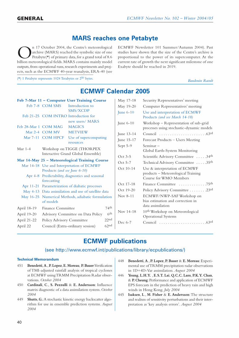
ECMWF Newsletter No. 102 – Winter 2004/05
40
GENERAL
ECMWF publications(see http://www.ecmwf.int/publications/library/ecpublications/)
Technical Memorandum
451 Benedetti,A.,P.Lopez,E.Moreau, P.Bauer:Verificationof TMI-adjusted rainfall analysis of tropical cyclonesat ECMWF using TRMM Precipitation Radar obser-vations. October 2004
450 Cardinali, C., S. Pezzulli & E. Andersson: Influencematrix diagnostic of a data assimilation system.October2004
449 Shutts,G.:A stochastic kinetic energy backscatter algo-rithm for use in ensemble prediction systems. August2004
448 Benedetti,A.,P. Lopez,P. Bauer & E. Moreau: Experi-mental use of TRMM precipitation radar observationsin 1D+4D-Var assimilation. August 2004
446 Yeung, L.H.Y. , E.S.T. Lai, Q.C.C. Lam, P.K.Y. Chan,& P. Cheung:Performance and application of ECMWFEPS forecasts in the prediction of heavy rain and highwinds in Hong Kong. July 2004
445 Isaksen, L., M. Fisher & E. Andersson:The structureand realism of sensitivity perturbations and their inter-pretation as ‘key analysis errors’. August 2004
On 17 October 2004, the Centre’s meteorologicalarchive (MARS) reached the symbolic size of onePetabyte(*) of primary data, for a grand total of 8.6
billion meteorological fields. MARS contains mainly modeloutputs, from operational runs, research experiments and proj-ects, such as the ECMWF 40-year reanalysis, ERA-40 (see
MARS reaches one PetabyteECMWF Newsletter 101 Summer/Autumn 2004). Paststudies have shown that the size of the Centre’s archive isproportional to the power of its supercomputer. At thecurrent rate of growth the next significant milestone of oneExabyte should be reached in 2019.
(*) 1 Petabyte represents 1024 Terabytes or 250 bytes.Baudouin Raoult
ECMWF Calendar 2005Feb 7-Mar 11 – Computer User Training Course
Feb 7-8 COM SMS Introduction to SMS/XCDP
Feb 21-25 COM INTRO Introduction fornew users/ MARS
Feb 28-Mar 1 COM MAG MAGICSMar 2-4 COM MV METVIEW
Mar 7-11 COM HPCF Use of supercomputing resources
Mar 1-4 Workshop on TIGGE (THORPEXInteractive Grand Global Ensemble)
Mar 14-May 25 – Meteorological Training CourseMar 14-18 Use and Interpretation of ECMWF
Products (and see June 6-10)Apr 4-8 Predictability, diagnostics and seasonal
forecastingApr 11-21 Parametrization of diabatic processesMay 4-13 Data assimilation and use of satellite data
May 16-25 Numerical Methods, adiabatic formulationof models
April 18-19 Finance Committee 74th
April 19-20 Advisory Committee on Data Policy 6th
April 21-22 Policy Advisory Committee 22nd
April 22 Council (Extra-ordinary session) 62nd
May 17-18 Security Representatives’ meeting
May 19-20 Computer Representatives’ meeting
June 6-10 Use and interpretation of ECMWFProducts (and see March 14-18)
June 6-10 Workshop – Representation of sub-gridprocesses using stochastic-dynamic models
June 13-14 Council . . . . . . . . . . . . . . . . . . . . . .63rd
June 15-17 Forecast Products – Users Meeting
Sept 5-9 Seminar –Global Earth-System Monitoring
Oct 3-5 Scientific Advisory Committee . . . . .34th
Oct 5-7 Technical Advisory Committee . . . . .35th
Oct 10-14 Use & interpretation of ECMWFproducts – Meteorological TrainingCourse for WMO Members
Oct 17-18 Finance Committee . . . . . . . . . . . . .75th
Oct 19-20 Policy Advisory Committee . . . . . . . .23rd
Nov 8-11 ECMWF/NWP-SAF Workshop onbias estimation and correction indata assimilation
Nov 14-18 10th Workshop on MeteorologicalOperational Systems
Dec 6-7 Council . . . . . . . . . . . . . . . . . . . . . .63rd
ECMWF Newsletter No. 102 – Winter 2004/05
MARS Archive Parameter Data
A database of all meteorological parameters that are in useat ECMWF and stored in our MARS data archive is nowavailable.
http://www.ecmwf.int/services/archive/d/parameters
High Performance Computing Workshop 2004
The biennial High Performance Computing in Meteorologyworkshop was held in October at ECMWF. It featuredpresentations from meteorological and research institutionsaround the world and computer manufacturers such as Cray,IBM, Intel, Fujitsu, NEC and SGI.
http://www.ecmwf.int/newsevents/meetings/workshops/2004/high_performance_computing-11th/
ECMWF High Performance Networking Workshop
ECMWF held the workshop for High-PerformanceTechnology in Local Area Networks on in September.Theobjective of the workshop was to bring together users andvendors of high-performance networking and interconnecttechnologies and share thoughts on the technology deploy-ments, trends and future directions with European focus.
http://www.ecmwf.int/newsevents/meetings/workshops/2004/High_Performance_Networking/
ECMWF/ELDAS Workshop
The closing workshop for the European Union projectELDAS (Development of a European Land Data AssimilationSystem to predict Floods and Droughts) was held inNovember at ECMWF
http://www.ecmwf.int/newsevents/meetings/workshops/2004/ELDAS_Land_surface_assimilation/
EU Research projects
Two new European Union project web sites are available onthe ECMWF Web Site under both the Framework 5 and 6Programmes.
- ECMWF is hosting Research Theme 1 (RT1) of theENSEMBLES project, coordinated by Paco Doblas-Reyes at ECMWF which will be the development of theEarth System Model.The ENSEMBLES project, co-ordi-nated by Dave Griggs, Director of Climate Research atthe Met Office, aims to develop an ensemble predictionsystem for climate change based on the principal state-of-the-art Earth System models developed in Europe,validated against gridded datasets, to produce for the firsttime, an objective probabilistic estimate of uncertainty infuture climate at the seasonal to decadal and longertimescales.
http://www.ecmwf.int/research/EU_projects/ENSEMBLES/
- The HALO project, coordinated by Tony Hollingsworthat ECMWF, will coordinate the architecture and systemintegration for the interacting parts of the Atmosphere,Land and Ocean thematic integrated projects (IP) inGMES, the Global Monitoring for Environment andSecurity initiative. Presentations from the HALO work-shop, held in November, are available.
http://www.ecmwf.int/research/EU_projects/HALO/
New items on the ECMWF web site
GENERAL
41
444 Drusch,M.,E.F.Wood,H. Gao & A.Thiele: Soil mois-ture retrieval during the Southern Great PlainsHydrology Experiment 1999:A comparison betweenexperimental remote sensing data and operationalproducts. June 2004
443 Drusch,M.,D.Vasiljevic & P.Viterbo:ECMWF’s globalsnow analysis:Assessment and revision based on satel-lite observations. June 2004
442 Meetschen,D.,B.van den Hurk,F.Ament & M.Drusch:Optimized surface radiation fields derived fromMETEOSAT imagery and a regional atmosphericmodel. July 2004
441 Ricci, S., A.T. Weaver, J.Vialard & P. Rogel: Incorp-orating state-dependent temperature-salinity constraintsin the background error covariance of variationalocean data assimilation. June 2004
440 Bourke,W.,R.Buizza and M. Naughton: Performanceof the ECMWF and the BoM ensemble systems inthe Southern Hemisphere. May 2004
ERA-40 Project Report Series
17 Kållberg, P., A. Simmons, S. Uppala & M. Fuentes:The ERA-40 archive. September 2004
Contract Reports to the European Space Agency
Janisková, M: Impact of EarthCARE products on numeri-cal weather prediction. July 2004Dethof, A: Monitoring and assimilation of MIPAS, SCIA-MACHY and GOMOS retrievals at ECMWF. November2004Watts, P.D., A.P. McNally, J-N. Thépaut, M. Matricardi,R.J. Engelen & N. Bormann: Measurement of seasonal CO2fluctuations from space. October 2004
Workshop Proceedings
ECMWF workshop on assimilation of high spectral reso-lution sounders in NWP. 28 June-1 July 2004Ninth workshop on meteorological operational systems.10-14 November 2003
Seminar Proceedings
Recent developments in numerical methods for atmos-pheric and ocean modelling. 6-10 September 2004
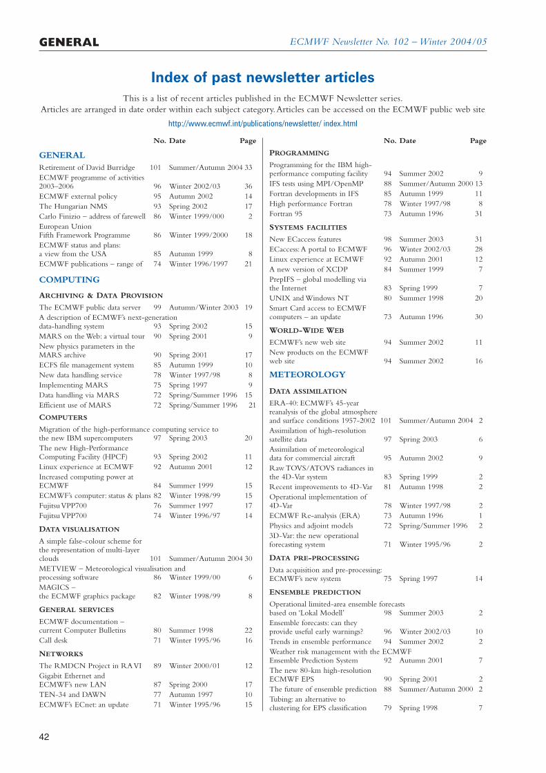
ECMWF Newsletter No. 102 – Winter 2004/05GENERAL
42
Index of past newsletter articlesThis is a list of recent articles published in the ECMWF Newsletter series.
Articles are arranged in date order within each subject category.Articles can be accessed on the ECMWF public web site
http://www.ecmwf.int/publications/newsletter/ index.html
No. Date Page
GENERALRetirement of David Burridge 101 Summer/Autumn 2004 33ECMWF programme of activities2003–2006 96 Winter 2002/03 36ECMWF external policy 95 Autumn 2002 14The Hungarian NMS 93 Spring 2002 17Carlo Finizio – address of farewell 86 Winter 1999/000 2European UnionFifth Framework Programme 86 Winter 1999/2000 18ECMWF status and plans:a view from the USA 85 Autumn 1999 8ECMWF publications – range of 74 Winter 1996/1997 21
COMPUTING
ARCHIVING & DATA PROVISION
The ECMWF public data server 99 Autumn/Winter 2003 19A description of ECMWF’s next-generationdata-handling system 93 Spring 2002 15MARS on the Web: a virtual tour 90 Spring 2001 9New physics parameters in theMARS archive 90 Spring 2001 17ECFS file management system 85 Autumn 1999 10New data handling service 78 Winter 1997/98 8Implementing MARS 75 Spring 1997 9Data handling via MARS 72 Spring/Summer 1996 15Efficient use of MARS 72 Spring/Summer 1996 21
COMPUTERS
Migration of the high-performance computing service tothe new IBM supercomputers 97 Spring 2003 20The new High-PerformanceComputing Facility (HPCF) 93 Spring 2002 11Linux experience at ECMWF 92 Autumn 2001 12Increased computing power atECMWF 84 Summer 1999 15ECMWF’s computer: status & plans 82 Winter 1998/99 15Fujitsu VPP700 76 Summer 1997 17Fujitsu VPP700 74 Winter 1996/97 14
DATA VISUALISATION
A simple false-colour scheme forthe representation of multi-layerclouds 101 Summer/Autumn 2004 30METVIEW – Meteorological visualisation andprocessing software 86 Winter 1999/00 6MAGICS –the ECMWF graphics package 82 Winter 1998/99 8
GENERAL SERVICES
ECMWF documentation –current Computer Bulletins 80 Summer 1998 22Call desk 71 Winter 1995/96 16
NETWORKS
The RMDCN Project in RA VI 89 Winter 2000/01 12Gigabit Ethernet and ECMWF’s new LAN 87 Spring 2000 17TEN-34 and DAWN 77 Autumn 1997 10ECMWF’s ECnet: an update 71 Winter 1995/96 15
No. Date Page
PROGRAMMING
Programming for the IBM high-performance computing facility 94 Summer 2002 9IFS tests using MPI/OpenMP 88 Summer/Autumn 2000 13Fortran developments in IFS 85 Autumn 1999 11High performance Fortran 78 Winter 1997/98 8Fortran 95 73 Autumn 1996 31
SYSTEMS FACILITIES
New ECaccess features 98 Summer 2003 31ECaccess:A portal to ECMWF 96 Winter 2002/03 28Linux experience at ECMWF 92 Autumn 2001 12A new version of XCDP 84 Summer 1999 7PrepIFS – global modelling viathe Internet 83 Spring 1999 7UNIX and Windows NT 80 Summer 1998 20Smart Card access to ECMWFcomputers – an update 73 Autumn 1996 30
WORLD-WIDE WEB
ECMWF’s new web site 94 Summer 2002 11New products on the ECMWFweb site 94 Summer 2002 16
METEOROLOGY
DATA ASSIMILATION
ERA-40: ECMWF’s 45-yearreanalysis of the global atmosphereand surface conditions 1957-2002 101 Summer/Autumn 2004 2Assimilation of high-resolutionsatellite data 97 Spring 2003 6Assimilation of meteorologicaldata for commercial aircraft 95 Autumn 2002 9Raw TOVS/ATOVS radiances inthe 4D-Var system 83 Spring 1999 2Recent improvements to 4D-Var 81 Autumn 1998 2Operational implementation of4D-Var 78 Winter 1997/98 2ECMWF Re-analysis (ERA) 73 Autumn 1996 1Physics and adjoint models 72 Spring/Summer 1996 23D-Var: the new operationalforecasting system 71 Winter 1995/96 2
DATA PRE-PROCESSING
Data acquisition and pre-processing:ECMWF’s new system 75 Spring 1997 14
ENSEMBLE PREDICTION
Operational limited-area ensemble forecastsbased on ‘Lokal Modell’ 98 Summer 2003 2Ensemble forecasts: can theyprovide useful early warnings? 96 Winter 2002/03 10Trends in ensemble performance 94 Summer 2002 2Weather risk management with the ECMWFEnsemble Prediction System 92 Autumn 2001 7The new 80-km high-resolutionECMWF EPS 90 Spring 2001 2The future of ensemble prediction 88 Summer/Autumn 2000 2Tubing: an alternative toclustering for EPS classification 79 Spring 1998 7
ECMWF Newsletter No. 102 – Winter 2004/05 GENERAL
43
No. Date Page
ENVIRONMENT
Environmental activities at ECMWF 99 Autumn/Winter 2003 18
FORECAST MODEL
Early delivery suite 101 Summer/Autumn 2004 21A major new cycle of the IFS:Cycle 25r4 97 Spring 2003 12Impact of the radiation transferscheme RRTM 91 Summer 2001 2Revised land-surface analysisscheme in the IFS 88 Summer/Autumn 2000 8The IFS cycle CY21r4 madeoperational in October 1999 87 Spring 2000 2Increased stratospheric resolution 82 Winter 1998/99 2Revisions to parametrizationsof physical processes 79 Spring 1998 2Integrated Forecasting Systemon the VPP700 75 Spring 1997 11Integrated Forecasting System –ten years 75 Spring 1997 2Improvements to 2mtemperature forecasts 73 Autumn 1996 2
FORECAST VERIFICATION
Systematic errors in theECMWF forecasting system 100 Spring 2004 14Verification of precipitation forecastsusing data from high-resolutionobservation networks 93 Spring 2002 2Verifying precipitation forecastsusing upscaled observations 87 Spring 2000 9Verification of ensemble prediction 72 Spring/Summer 1996 9
METEOROLOGICAL APPLICATIONS
European Flood Alert System 101 Summer/Autumn 2004 30Model predictions of the floods in theCzech Republic during August 2002:The forecaster’s perspective 97 Spring 2003 2Joining the ECMWF improvesthe quality of forecasts 94 Summer 2002 6Forecasts for the Karakoram mountains 92 Autumn 2001 3Breitling Orbiter: meteorologicalaspects of the balloon flightaround the world 84 Summer 1999 2Obtaining economic value fromthe EPS 80 Summer 1998 8
METEOROLOGICAL STUDIES
The exceptional warm anomaliesof summer 2003 99 Autumn/Winter 2003 2Record-breaking warm sea surfacetemperatures ofthe Mediterranean Sea 98 Summer 2003 30Breakdown of the stratosphericwinter polar vortex 96 Winter 2002/03 2Central European floods duringsummer 2002 96 Winter 2002/03 18Dreaming of a white Christmas! 93 Spring 2002 8Severe weather prediction using theECMWF EPS: the Europeanstorms of December 1999 89 Winter 2000/01 2Forecasting the tracks of tropicalcyclones over the western NorthPacific and the South China Sea 85 Autumn 1999 2January 1997 floods in Greece 76 Summer 1997 9Extreme rainfall predictionusing the ECMWF EPS 73 Autumn 1996 17
No. Date Page
OBSERVATIONS
Influence of observations in theoperational ECMWF system 76 Summer 1997 2
OCEAN AND WAVE MODELLING
Towards freak-wave predictionover the global oceans 100 Spring 2004 24Probabilistic forecasts for ocean waves 95 Autumn 2002 2ECMWF wave-model products 91 Summer 2001 9Potential benefits of ensembleprediction of waves 86 Winter 1999/00 3Wind-wave interaction 80 Summer 1998 2
MONTHLY FORECASTING
Monthly forecasting 100 Spring 2004 3
SEASONAL FORECASTING
DEMETER: Development of a Europeanmulti-model ensemble system forseasonal to interannual prediction 99 Autumn/Winter 2003 8The ECMWFseasonal forecasting system 98 Summer 2003 17Did the ECMWF seasonal forecastingmodel outperform a statistical modelover the last 15 years? 98 Summer 2003 26Seasonal forecasting at ECMWF 77 Autumn 1997 2
ECMWF Newsletter No. 102 – Winter 2004/05
Ext
DirectorDominique Marbouty 001
Deputy Director & Head of Administration DepartmentGerd Schultes 007
Head of Operations DepartmentWalter Zwieflhofer 003
Head of Research DepartmentPhilippe Bougeault 005
ECMWF switchboard 000
AdvisoryInternet mail addressed to [email protected] (+44 118 986 9450, marked User Support)
Computer DivisionDivision Head
050
Computer Operations Section HeadSylvia Baylis 301
Networking and Computer Security Section HeadMatteo Dell’Acqua 356
Servers and Desktops Section HeadRichard Fisker 355
Systems Software Section HeadNeil Storer 353
User Support Section HeadUmberto Modigliani 382
User Support Staff
John Greenaway 385Norbert Kreitz 381Dominique Lucas 386Carsten Maaß 389Pam Prior 384
Computer OperationsCall Desk 303
Call Desk email: [email protected]
Console - Shift Leaders 803Console fax number +44 118 949 9840Console email: [email protected]
Fault reporting - Call Desk 303Registration - Call Desk 303Service queries - Call Desk 303Tape Requests - Tape Librarian 315
Software libraries (eclib, nag, etc.)John Greenaway 385
Ext
ECMWF library & documentation distributionEls Kooij-Connally 751
Meteorological Division
Division HeadHorst Böttger 060
Applications Section HeadAlfred Hofstadler 400
Data and Services HeadBaudouin Raoult 404
Graphics Section HeadJens Daabeck 375
Operations Section HeadFrançois Lalaurette 420
Meteorological AnalystsAntonio Garcia Mendez 424Federico Grazzini 421Anna Ghelli 425
Meteorological Operations Room 426
Data DivisionDivision HeadAdrian Simmons 700
Data Assimilation Section HeadErik Andersson 627
Satellite Section HeadJean-Nöel Thépaut 621
Reanalysis Project (ERA)Saki Uppala 366
Probability Forecasting & Diagnostics DivisionDivision HeadTim Palmer 600
Seasonal Forecasting HeadDavid Anderson 706
Model DivisionDivision HeadMartin Miller 070
Numerical Aspects Section HeadMariano Hortal 147
Physical Aspects Section HeadAnton Beljaars 035
Ocean Waves Section HeadPeter Janssen 116
Education & TrainingRenate Hagedorn 257
GMES CoordinatorAnthony Hollingsworth 824
Useful names and telephone numbers within ECMWFTelephone number of an individual at the Centre is:
International: +44 118 949 9 + three digit extensionUK: (0118) 949 9 + three digit extensionInternal: 2 + three digit extension
e.g. the Director’s number is:+44 118 949 9001 (international),(0118) 949 9001 (UK) and 2001 (internal).
E-mailThe e-mail address of an individual at the Centre is:[email protected]
e.g. the Director’s address is: [email protected]
For double-barrelled names use a hyphene.g. [email protected]
Internet web siteECMWF’s public web site is: http://www.ecmwf.int
GENERAL
44