Gaussian Mixture Model

CS 224S / LINGUIST 281Speech Recognition, Synthesis, and

Dialogue

Dan Jurafsky

Lecture 10: Acoustic Modeling

IP Notice:

Outline for Today• Speech Recognition Architectural Overview• Hidden Markov Models in general and for speech Forward Viterbi Decoding

• How this fits into the ASR component of course Jan 27 HMMs, Forward, Viterbi, Jan 29 Baum-Welch (Forward-Backward) Feb 3: Feature Extraction, MFCCs, start of AM (VQ) Feb 5: Acoustic Modeling: GMMs Feb 10: N-grams and Language Modeling Feb 24: Search and Advanced Decoding Feb 26: Dealing with Variation Mar 3: Dealing with Disfluencies

Outline for Today• Acoustic Model

Increasingly sophisticated models Acoustic Likelihood for each state:

Gaussians Multivariate Gaussians Mixtures of Multivariate Gaussians

Where a state is progressively: CI Subphone (3ish per phone) CD phone (=triphones) State-tying of CD phone

• If Time: Evaluation Word Error Rate

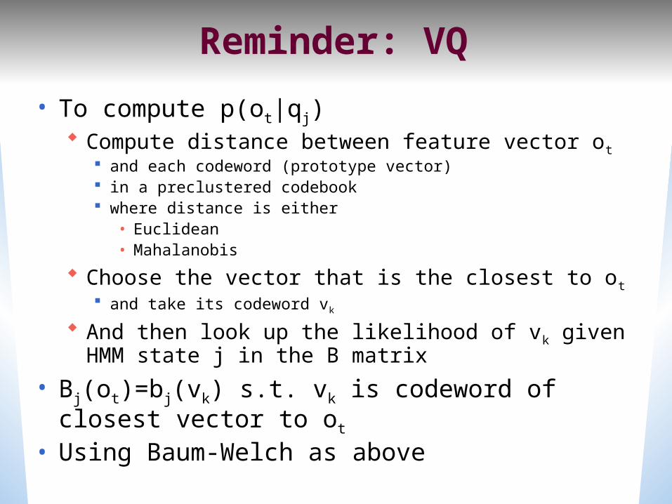
Reminder: VQ• To compute p(ot|qj)

Compute distance between feature vector ot and each codeword (prototype vector) in a preclustered codebook where distance is either

• Euclidean• Mahalanobis

Choose the vector that is the closest to ot and take its codeword vk

And then look up the likelihood of vk given HMM state j in the B matrix

• Bj(ot)=bj(vk) s.t. vk is codeword of closest vector to ot

• Using Baum-Welch as above

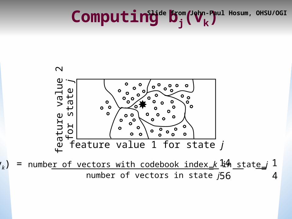
Computing bj(vk)

feature value 1 for state jfeature value 2

for state

j

• bj(vk) = number of vectors with codebook index k in state j number of vectors in state j

= =14 156 4

Slide from John-Paul Hosum, OHSU/OGI

Summary: VQ• Training:

Do VQ and then use Baum-Welch to assign probabilities to each symbol

• Decoding: Do VQ and then use the symbol probabilities in decoding

Directly Modeling Continuous Observations

• Gaussians Univariate Gaussians

Baum-Welch for univariate Gaussians Multivariate Gaussians

Baum-Welch for multivariate Gausians Gaussian Mixture Models (GMMs)

Baum-Welch for GMMs

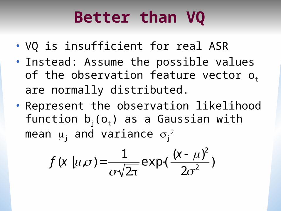
Better than VQ• VQ is insufficient for real ASR• Instead: Assume the possible values of the observation feature vector ot are normally distributed.

• Represent the observation likelihood function bj(ot) as a Gaussian with mean j and variance j

2

f(x |,) 1 2

exp( (x )22 2 )

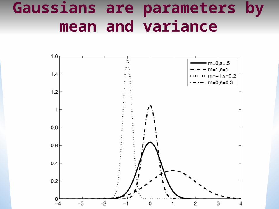
Gaussians are parameters by mean and variance

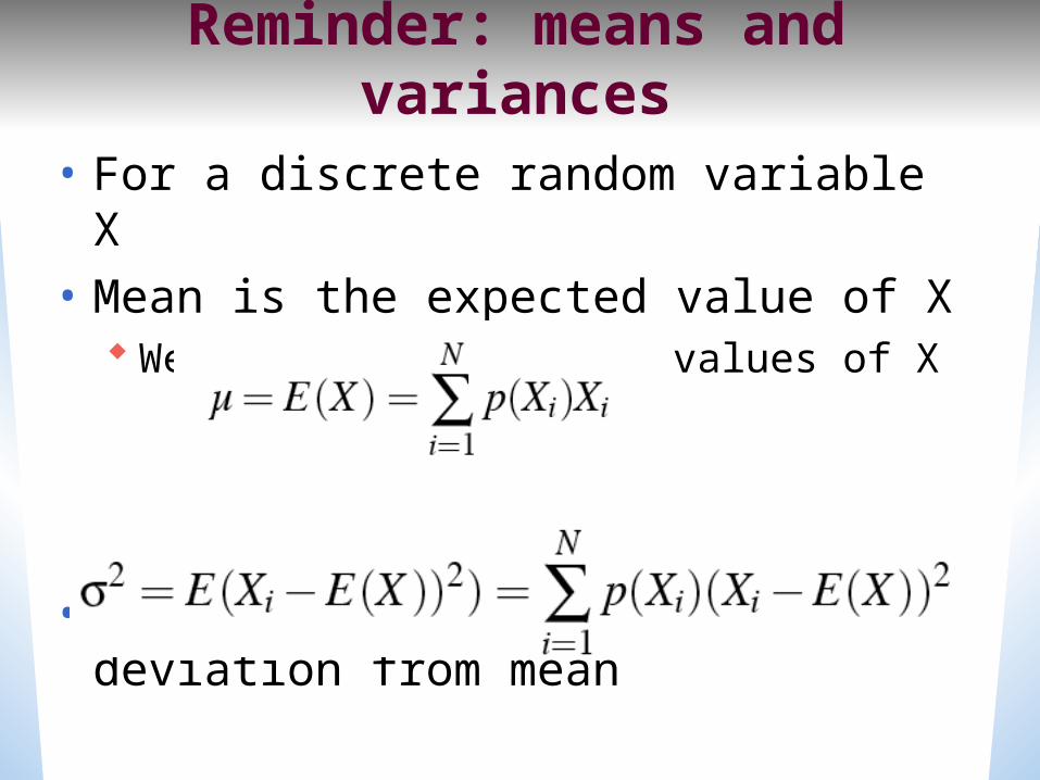
• For a discrete random variable X

• Mean is the expected value of X Weighted sum over the values of X

• Variance is the squared average deviation from mean

Reminder: means and variances

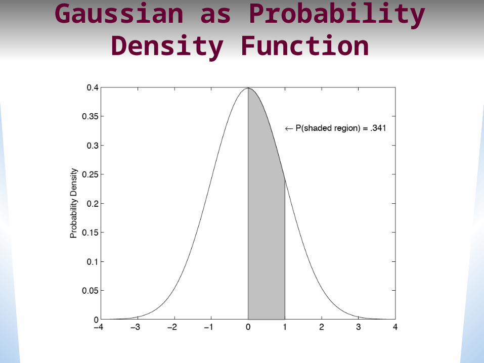
Gaussian as Probability Density Function

Gaussian PDFs• A Gaussian is a probability density function; probability is area under curve.

• To make it a probability, we constrain area under curve = 1.

• BUT… We will be using “point estimates”; value of Gaussian at point.

• Technically these are not probabilities, since a pdf gives a probability over a interval, needs to be multiplied by dx

• As we will see later, this is ok since the same value is omitted from all Gaussians, so argmax is still correct.

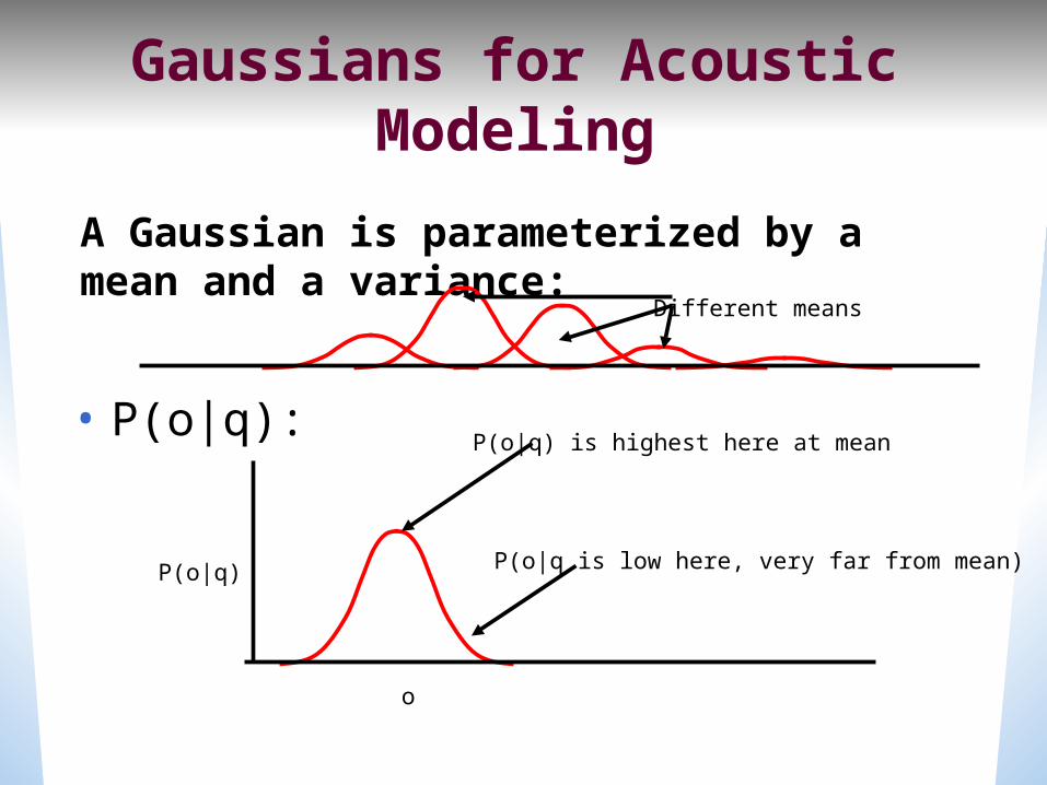
Gaussians for Acoustic Modeling

• P(o|q):

P(o|q)

o

P(o|q) is highest here at mean

P(o|q is low here, very far from mean)

A Gaussian is parameterized by a mean and a variance:

Different means

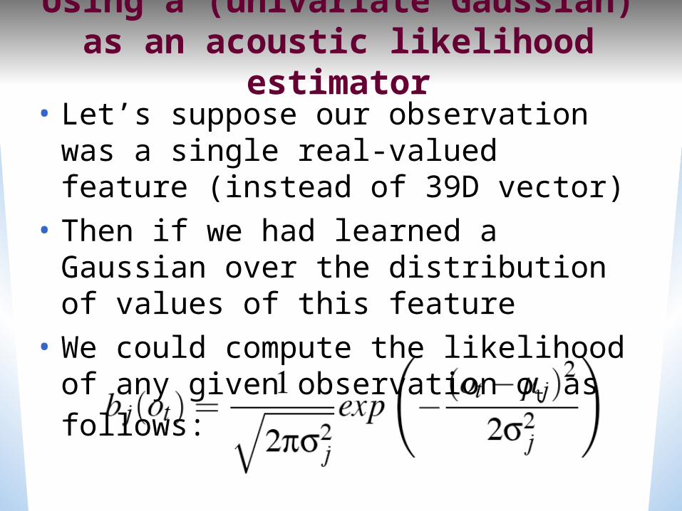
Using a (univariate Gaussian) as an acoustic likelihood

estimator• Let’s suppose our observation was a single real-valued feature (instead of 39D vector)

• Then if we had learned a Gaussian over the distribution of values of this feature

• We could compute the likelihood of any given observation ot as follows:

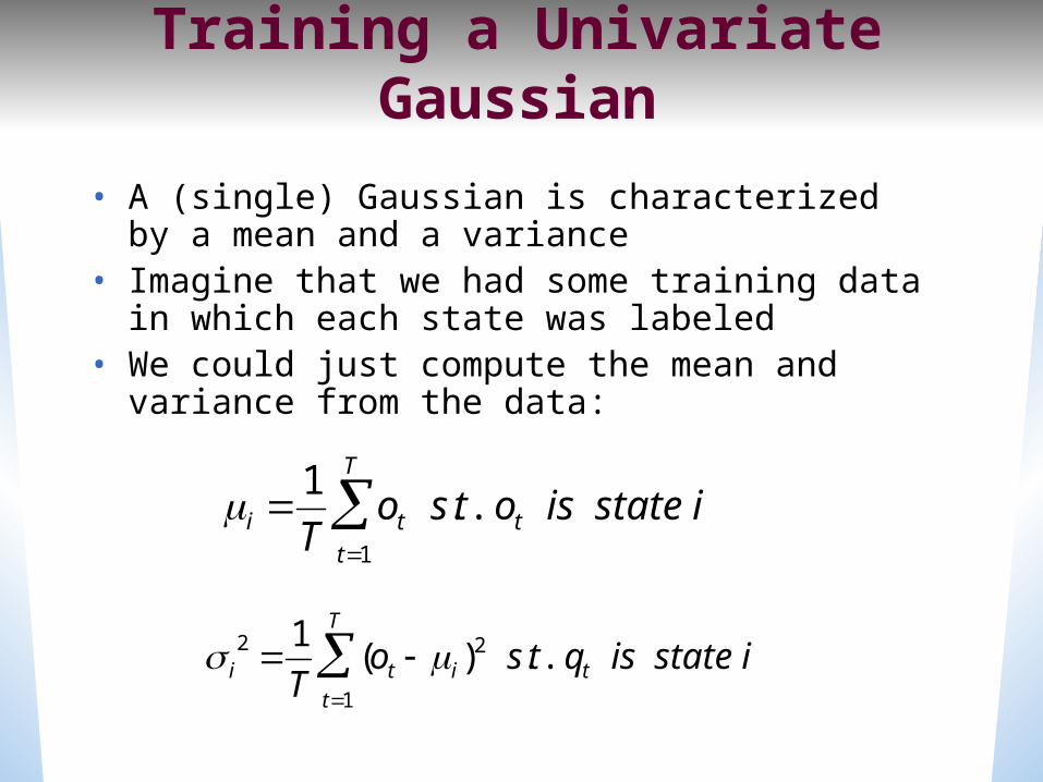
Training a Univariate Gaussian

• A (single) Gaussian is characterized by a mean and a variance

• Imagine that we had some training data in which each state was labeled

• We could just compute the mean and variance from the data:

i 1T

ott1

T

s.t. ot is state i

i2

1T

(ott1

T

i)2 s.t. qt is state i

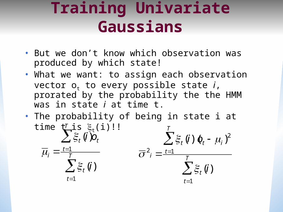
Training Univariate Gaussians

• But we don’t know which observation was produced by which state!

• What we want: to assign each observation vector ot to every possible state i, prorated by the probability the the HMM was in state i at time t.

• The probability of being in state i at time t is t(i)!!

2i t(i)(ot i)2

t1

T

t(i)t1

T

i t(i)ot

t1

T

t(i)t1

T

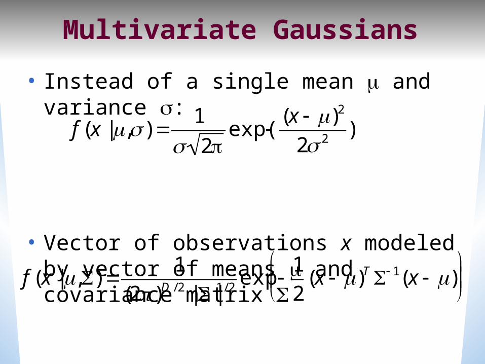
Multivariate Gaussians• Instead of a single mean and variance :

• Vector of observations x modeled by vector of means and covariance matrix

f(x |,) 1 2

exp( (x )22 2 )

f(x |,) 1(2)D /2 | |1/2 exp

12(x )T 1(x )

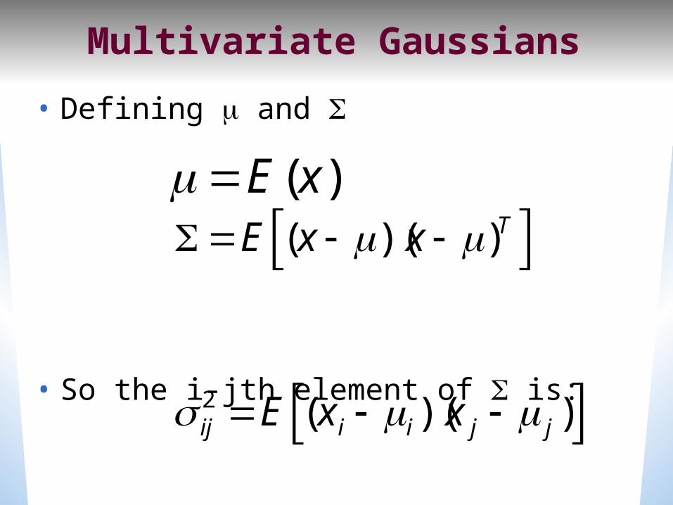
Multivariate Gaussians• Defining and

• So the i-jth element of is:

E (x)

E (x )(x )T

ij2 E (xi i)(x j j)

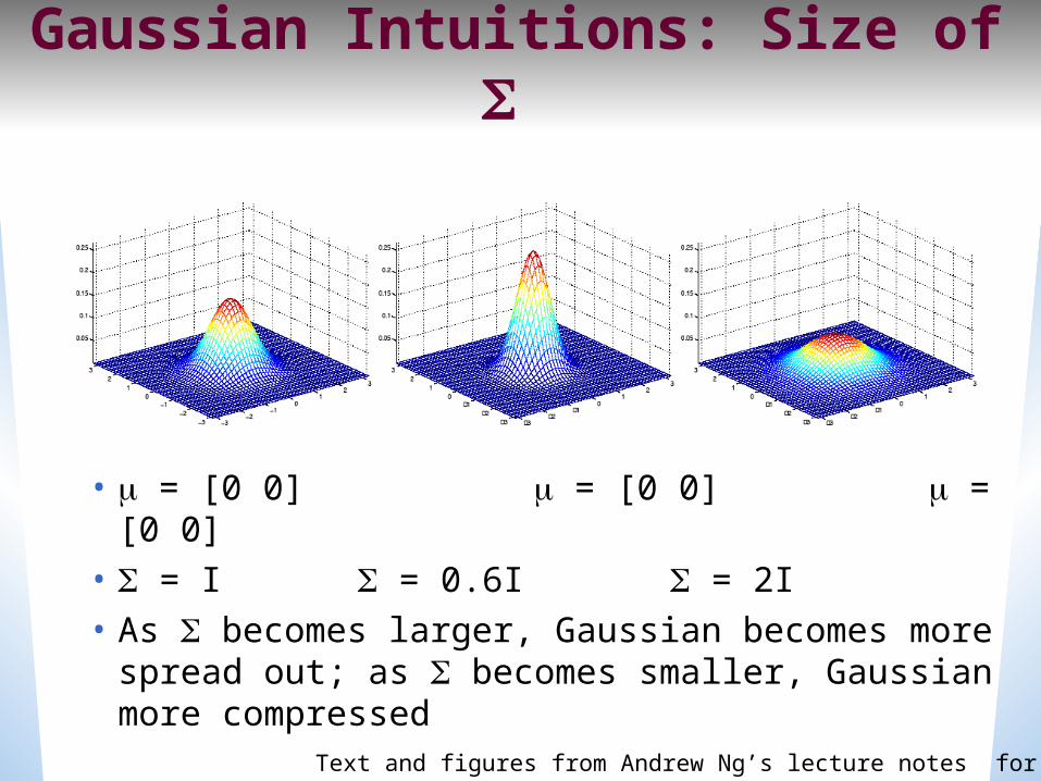
Gaussian Intuitions: Size of

• = [0 0] = [0 0] = [0 0]

• = I = 0.6I = 2I• As becomes larger, Gaussian becomes more spread out; as becomes smaller, Gaussian more compressed

Text and figures from Andrew Ng’s lecture notes for CS229

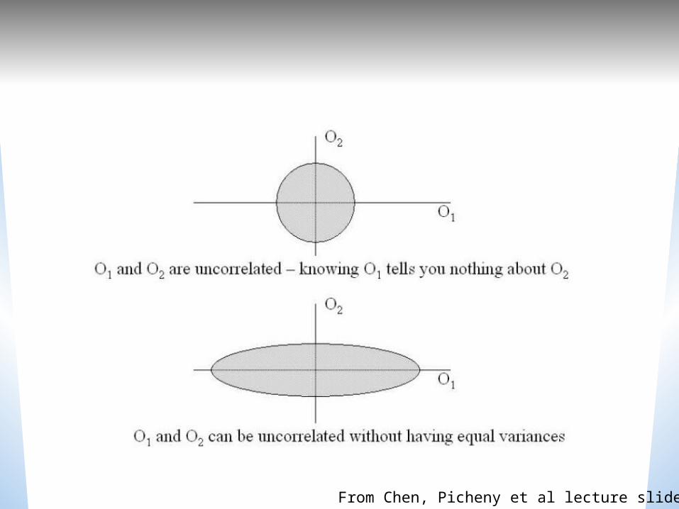
From Chen, Picheny et al lecture slides

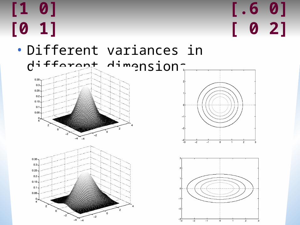
[1 0] [.6 0][0 1] [ 0 2]• Different variances in different dimensions

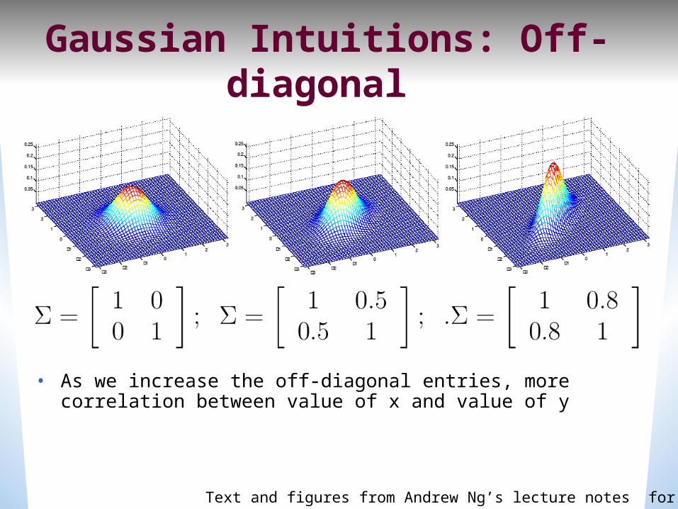
Gaussian Intuitions: Off-diagonal

• As we increase the off-diagonal entries, more correlation between value of x and value of y


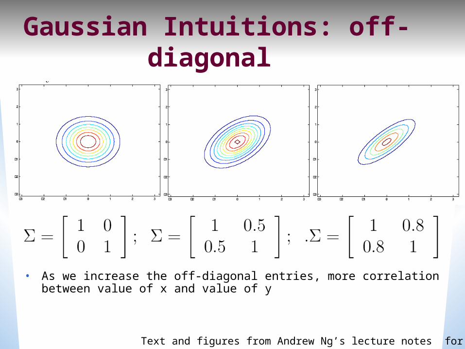
Gaussian Intuitions: off-diagonal

• As we increase the off-diagonal entries, more correlation between value of x and value of y


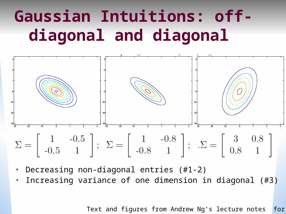
Gaussian Intuitions: off-diagonal and diagonal

• Decreasing non-diagonal entries (#1-2)• Increasing variance of one dimension in diagonal (#3)


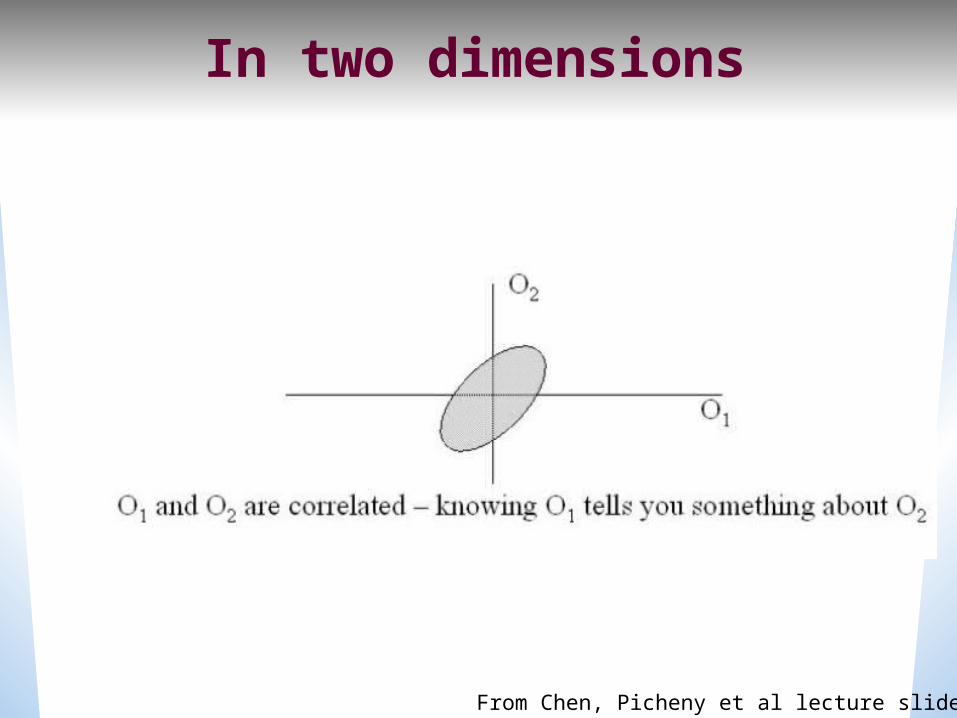
In two dimensions

From Chen, Picheny et al lecture slides

But: assume diagonal covariance

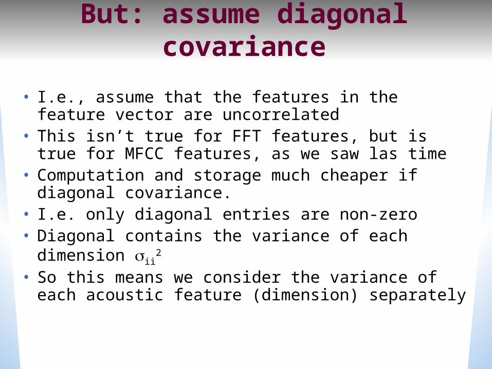
• I.e., assume that the features in the feature vector are uncorrelated

• This isn’t true for FFT features, but is true for MFCC features, as we saw las time

• Computation and storage much cheaper if diagonal covariance.

• I.e. only diagonal entries are non-zero• Diagonal contains the variance of each dimension ii

2

• So this means we consider the variance of each acoustic feature (dimension) separately

Diagonal covariance

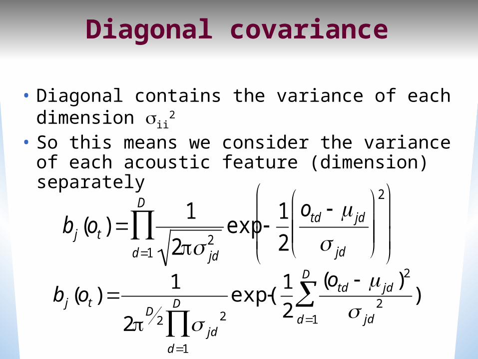
• Diagonal contains the variance of each dimension ii

2

• So this means we consider the variance of each acoustic feature (dimension) separately

bj(ot)1

2 jd2exp

12

otd jd

jd

2

d1

D

bj(ot)1

2D 2 jd2

d1

D

exp( 12

(otd jd)2 jd

2d1

D

)

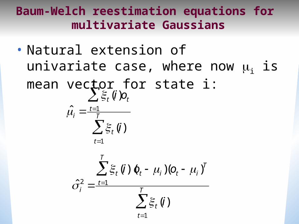
Baum-Welch reestimation equations for multivariate Gaussians

• Natural extension of univariate case, where now i is mean vector for state i:

ˆ i2

t(i)(ot i)t1

T

(ot i)T

t(i)t1

T

ˆ i t(i)ot

t1

T

t(i)t1

T

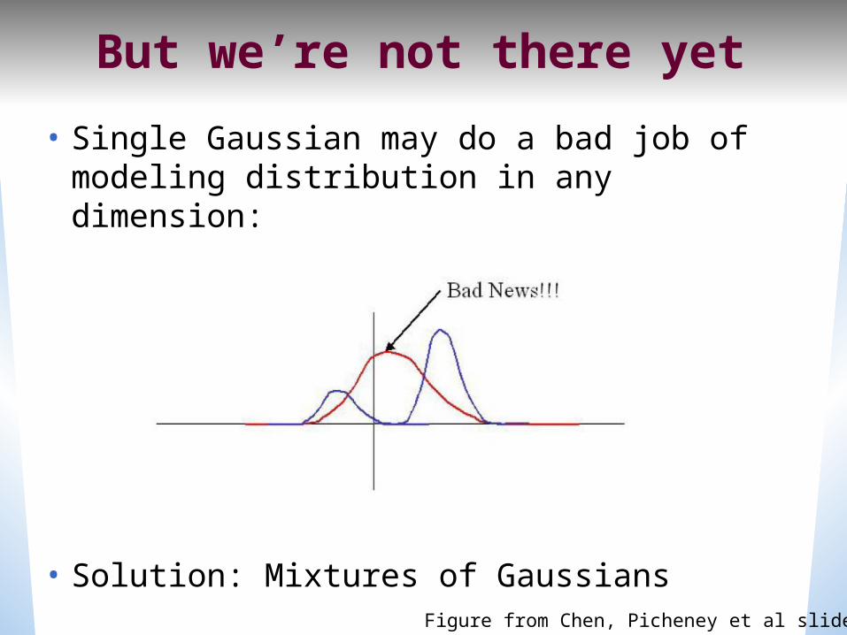
But we’re not there yet• Single Gaussian may do a bad job of modeling distribution in any dimension:

• Solution: Mixtures of GaussiansFigure from Chen, Picheney et al slides

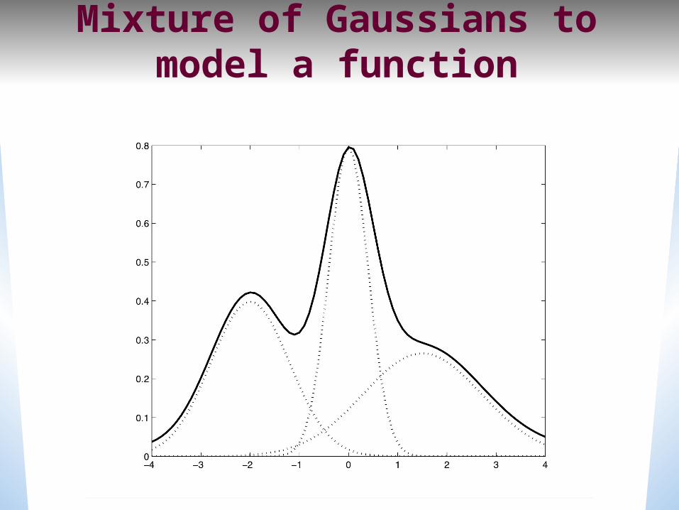
Mixture of Gaussians to model a function

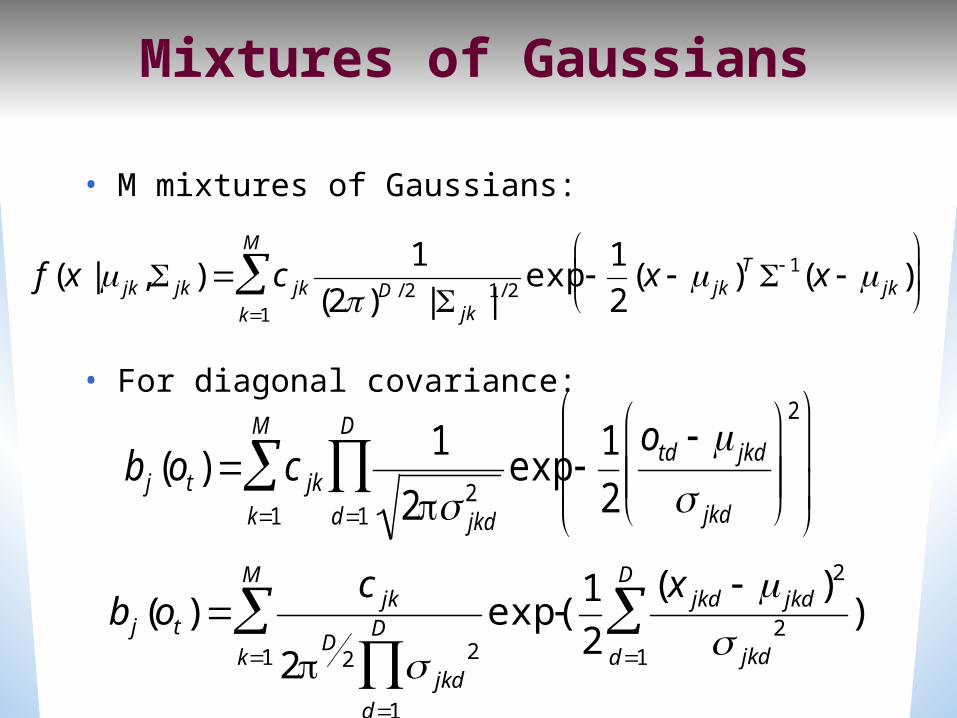
Mixtures of Gaussians

• M mixtures of Gaussians:

• For diagonal covariance:

bj(ot)c jk

2D 2 jkd2

d1

D

exp( 12

(x jkd jkd)2 jkd

2d1

D

)k1

M

bj(ot) c jkk1

M

12 jkd

2exp 12

otd jkd

jkd

2

d1

D

f(x | jk, jk) c jkk1

M

1(2)D /2 | jk |1/2

exp 12(x jk)T 1(x jk)

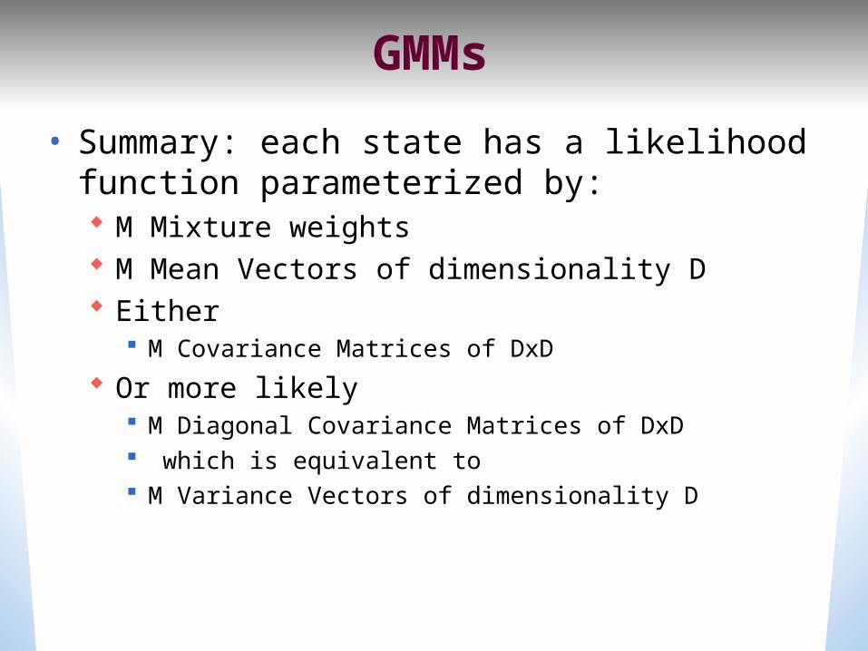
GMMs• Summary: each state has a likelihood function parameterized by: M Mixture weights M Mean Vectors of dimensionality D Either

M Covariance Matrices of DxD Or more likely

M Diagonal Covariance Matrices of DxD which is equivalent to M Variance Vectors of dimensionality D

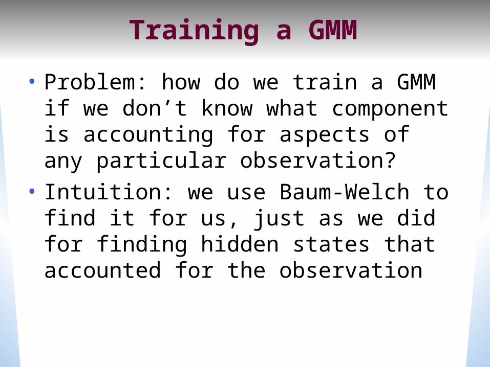
Training a GMM• Problem: how do we train a GMM if we don’t know what component is accounting for aspects of any particular observation?

• Intuition: we use Baum-Welch to find it for us, just as we did for finding hidden states that accounted for the observation

10/10/22 34

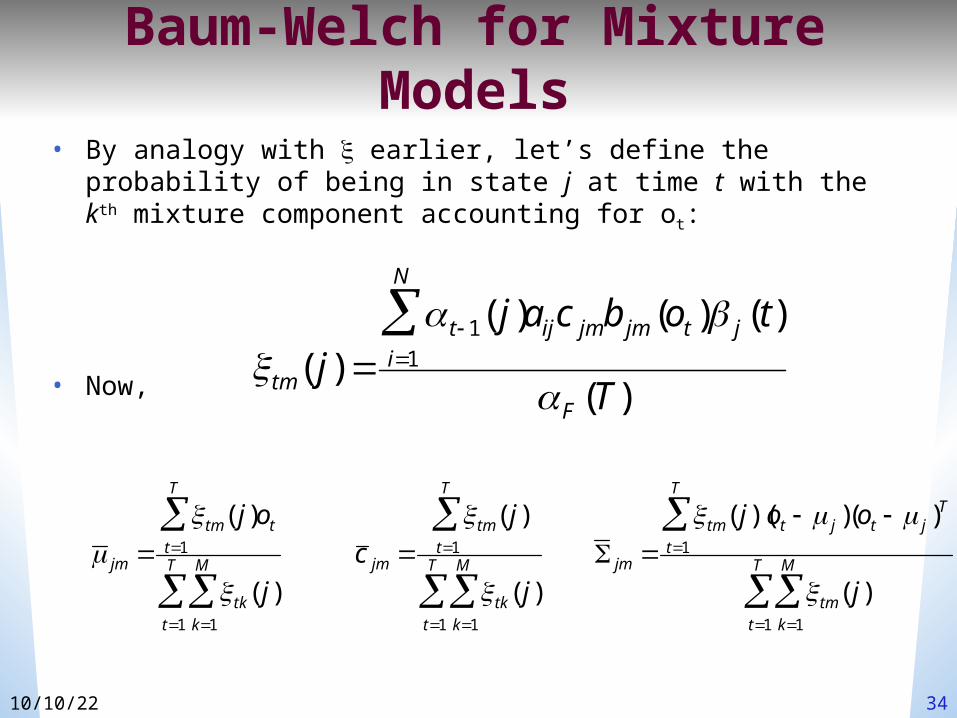
Baum-Welch for Mixture Models

• By analogy with earlier, let’s define the probability of being in state j at time t with the kth mixture component accounting for ot:

• Now,

tm(j) t1(j)

i1

N

aijc jmbjm(ot) j(t)

F (T)

jm tm(j)ot

t1

T

tk(j)k1

M

t1

T

c jm tm(j)

t1

T

tk(j)k1

M

t1

T

jm tm(j)(ot j)

t1

T

(ot j)T

tm(j)k1

M

t1

T

10/10/22 35

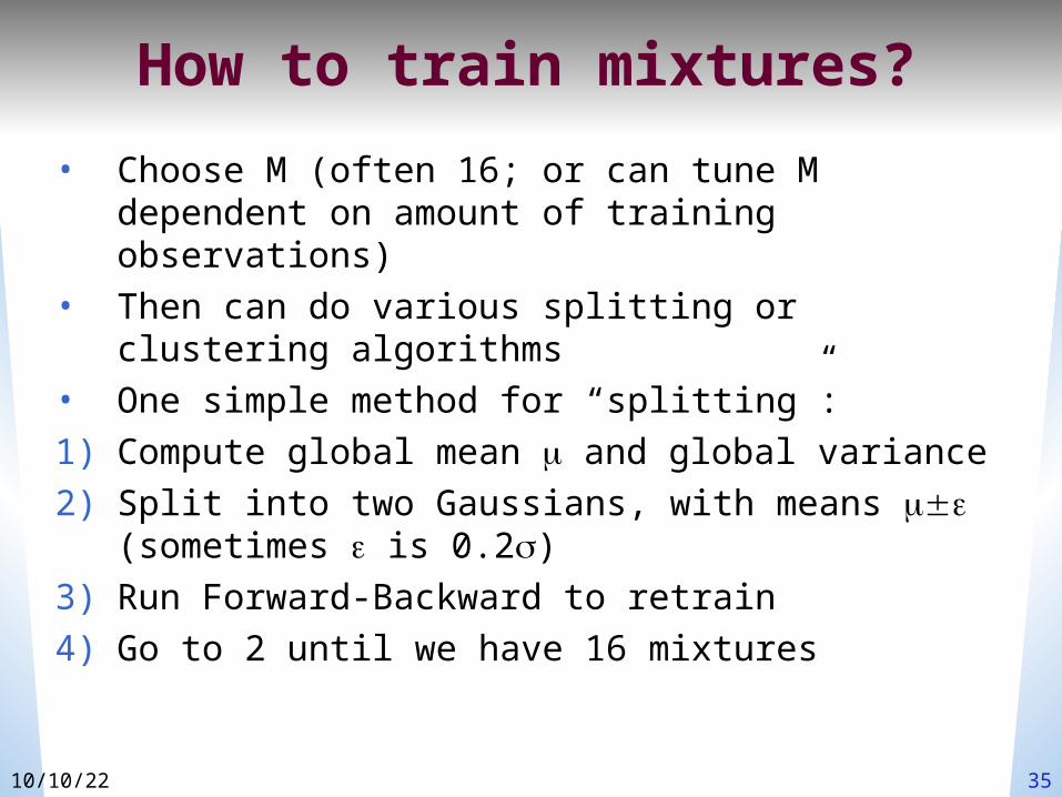
How to train mixtures?• Choose M (often 16; or can tune M

dependent on amount of training observations)

• Then can do various splitting or clustering algorithms

• One simple method for “splitting”:1) Compute global mean and global variance2) Split into two Gaussians, with means

(sometimes is 0.2)3) Run Forward-Backward to retrain 4) Go to 2 until we have 16 mixtures

10/10/22 CS 224S Winter 2007 36

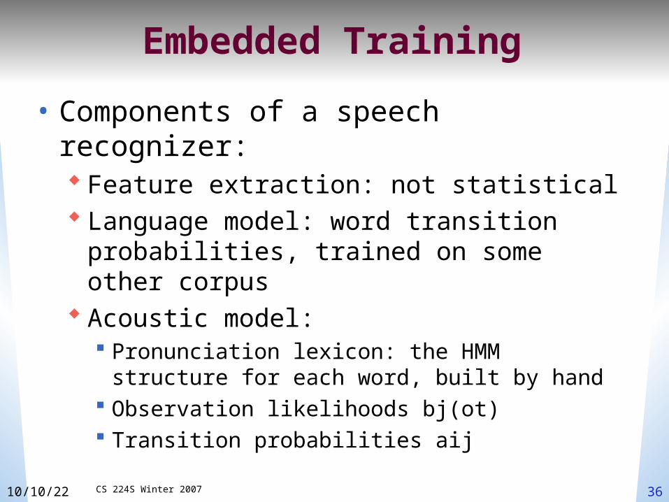
Embedded Training• Components of a speech recognizer: Feature extraction: not statistical Language model: word transition probabilities, trained on some other corpus

Acoustic model: Pronunciation lexicon: the HMM structure for each word, built by hand

Observation likelihoods bj(ot) Transition probabilities aij

10/10/22 CS 224S Winter 2007 37

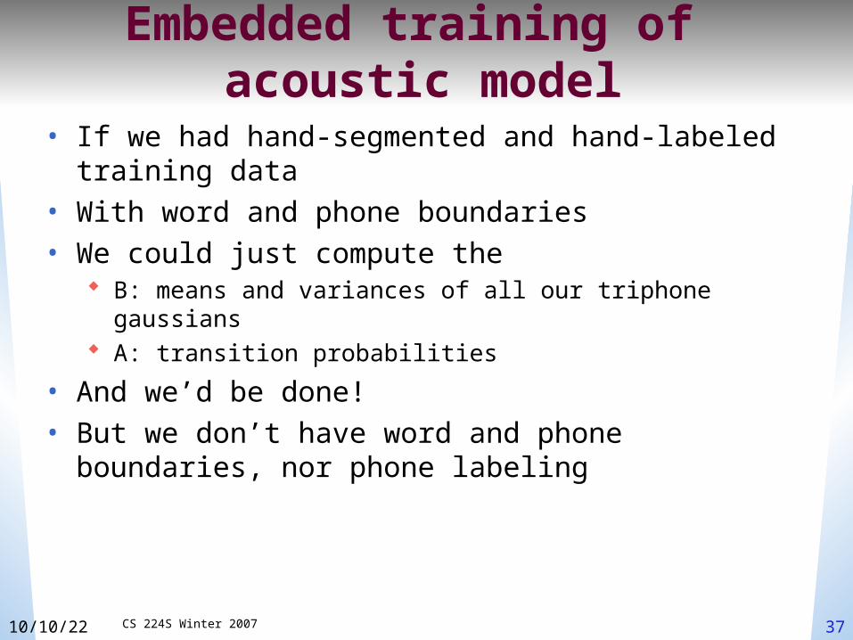
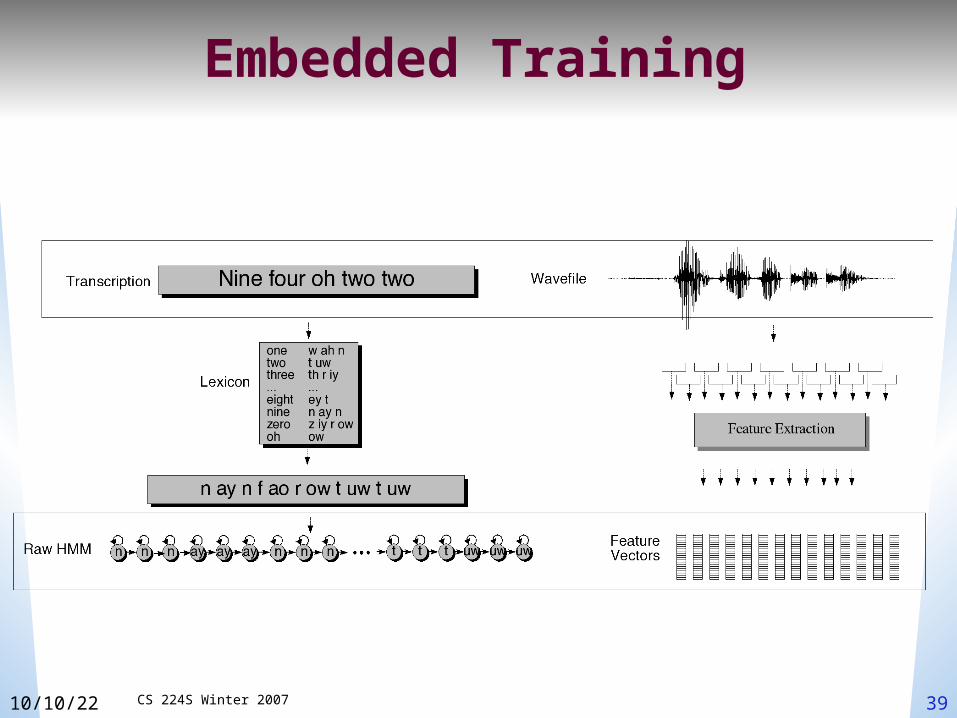
Embedded training of acoustic model

• If we had hand-segmented and hand-labeled training data

• With word and phone boundaries• We could just compute the

B: means and variances of all our triphone gaussians

A: transition probabilities• And we’d be done!• But we don’t have word and phone boundaries, nor phone labeling

10/10/22 CS 224S Winter 2007 38

Embedded training• Instead:

We’ll train each phone HMM embedded in an entire sentence

We’ll do word/phone segmentation and alignment automatically as part of training process

10/10/22 CS 224S Winter 2007 39

Embedded Training

10/10/22 40

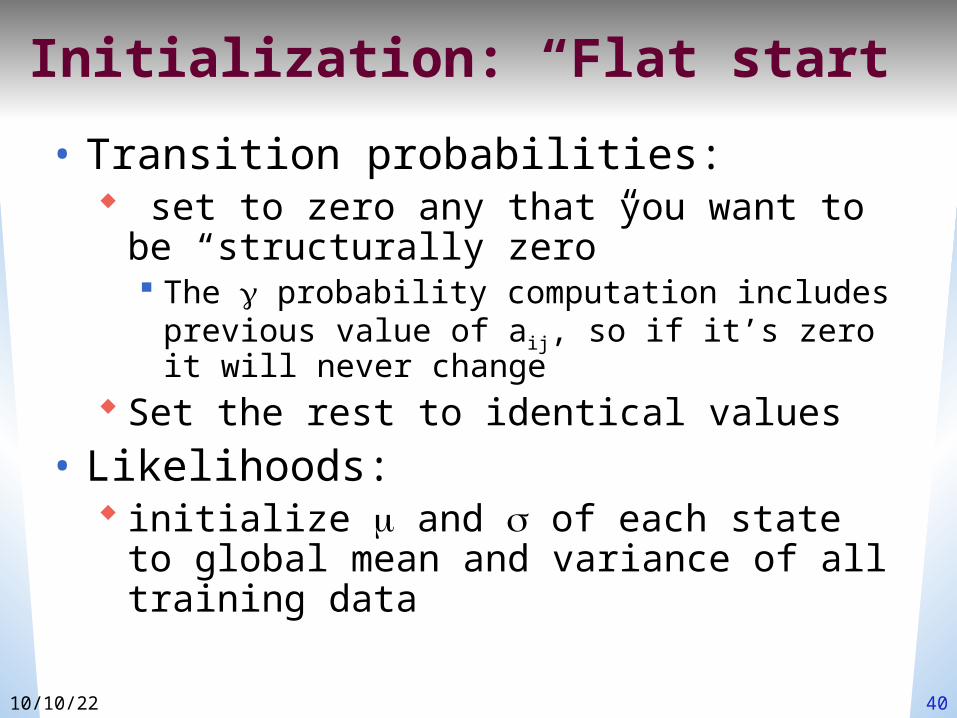
Initialization: “Flat start”• Transition probabilities:

set to zero any that you want to be “structurally zero” The probability computation includes previous value of aij, so if it’s zero it will never change

Set the rest to identical values• Likelihoods:

initialize and of each state to global mean and variance of all training data

10/10/22 41

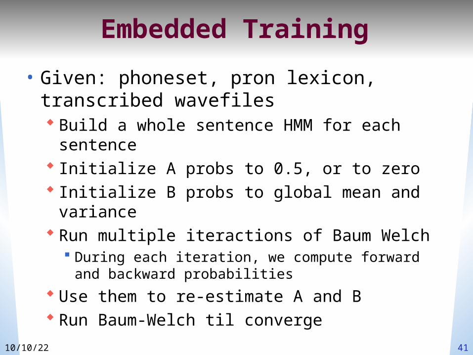
Embedded Training• Given: phoneset, pron lexicon, transcribed wavefiles Build a whole sentence HMM for each sentence

Initialize A probs to 0.5, or to zero Initialize B probs to global mean and variance

Run multiple iteractions of Baum Welch During each iteration, we compute forward and backward probabilities

Use them to re-estimate A and B Run Baum-Welch til converge

10/10/22 CS 224S Winter 2007 42

Viterbi training• Baum-Welch training says:

We need to know what state we were in, to accumulate counts of a given output symbol ot

We’ll compute I(t), the probability of being in state i at time t, by using forward-backward to sum over all possible paths that might have been in state i and output ot.

• Viterbi training says: Instead of summing over all possible paths, just take the single most likely path

Use the Viterbi algorithm to compute this “Viterbi” path

Via “forced alignment”

10/10/22 CS 224S Winter 2007 43

Forced Alignment• Computing the “Viterbi path” over the training data is called “forced alignment”

• Because we know which word string to assign to each observation sequence.

• We just don’t know the state sequence.

• So we use aij to constrain the path to go through the correct words

• And otherwise do normal Viterbi• Result: state sequence!

10/10/22 CS 224S Winter 2007 44

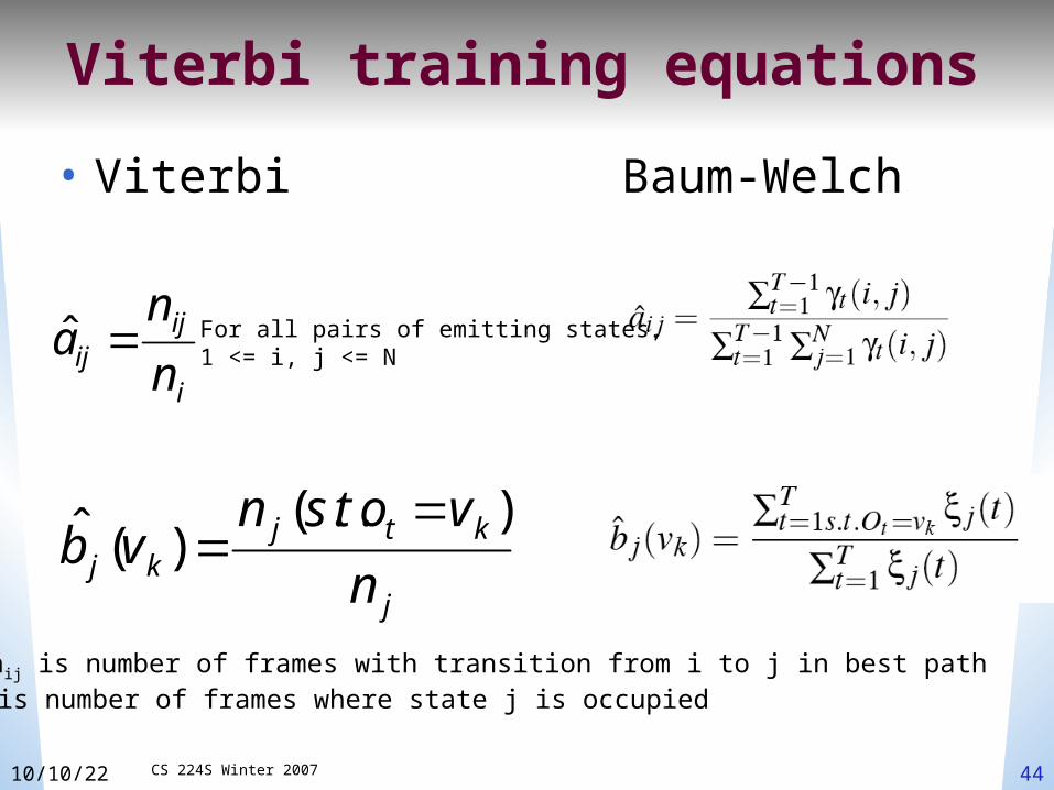
Viterbi training equations• Viterbi Baum-Welch

ˆ b j(vk)n j(s.t.ot vk)

n j

ˆ a ij nij

ni

For all pairs of emitting states, 1 <= i, j <= N

Where nij is number of frames with transition from i to j in best pathAnd nj is number of frames where state j is occupied

10/10/22 CS 224S Winter 2007 45

Viterbi Training• Much faster than Baum-Welch• But doesn’t work quite as well• But the tradeoff is often worth it.

10/10/22 CS 224S Winter 2007 46

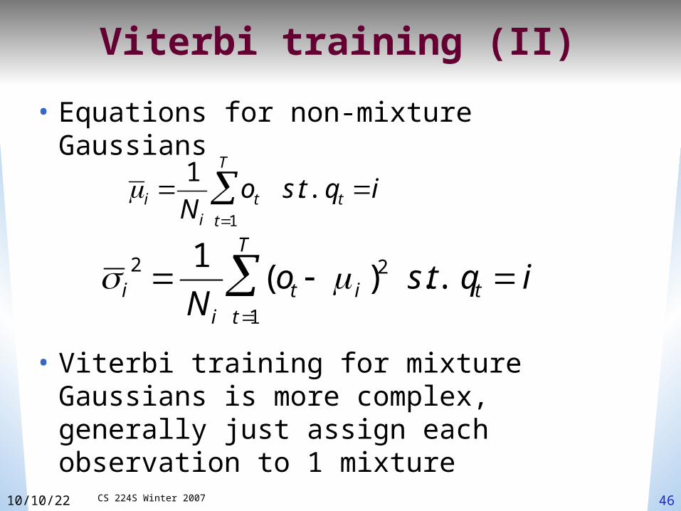
Viterbi training (II)• Equations for non-mixture Gaussians

• Viterbi training for mixture Gaussians is more complex, generally just assign each observation to 1 mixture

i2

1Ni

(ott1

T

i )2 s.t. qt i

i 1Ni

ot s.t. qt it1

T

10/10/22 CS 224S Winter 2007 47

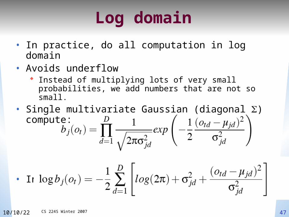
Log domain• In practice, do all computation in log domain

• Avoids underflow Instead of multiplying lots of very small probabilities, we add numbers that are not so small.

• Single multivariate Gaussian (diagonal ) compute:

• In log space:

10/10/22 CS 224S Winter 2007 48

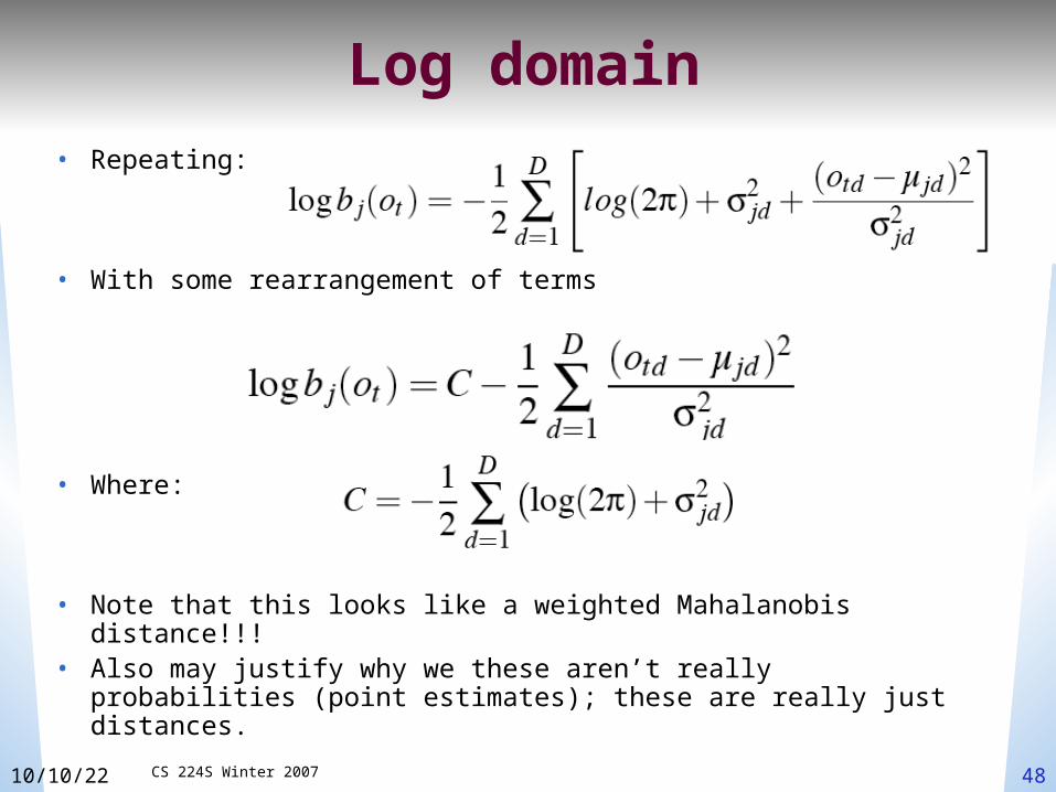
• Repeating:

• With some rearrangement of terms

• Where:

• Note that this looks like a weighted Mahalanobis distance!!!

• Also may justify why we these aren’t really probabilities (point estimates); these are really just distances.

Log domain

Evaluation• How to evaluate the word string output by a speech recognizer?

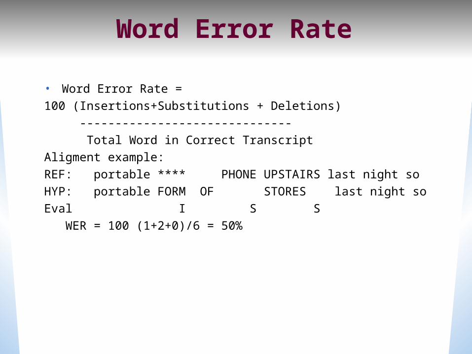
Word Error Rate

• Word Error Rate = 100 (Insertions+Substitutions + Deletions) ------------------------------ Total Word in Correct TranscriptAligment example:REF: portable **** PHONE UPSTAIRS last night soHYP: portable FORM OF STORES last night soEval I S S WER = 100 (1+2+0)/6 = 50%

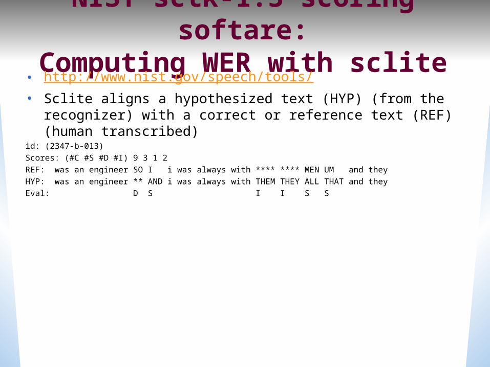
NIST sctk-1.3 scoring softare:

Computing WER with sclite• http://www.nist.gov/speech/tools/• Sclite aligns a hypothesized text (HYP) (from the

recognizer) with a correct or reference text (REF) (human transcribed)

id: (2347-b-013)Scores: (#C #S #D #I) 9 3 1 2REF: was an engineer SO I i was always with **** **** MEN UM and theyHYP: was an engineer ** AND i was always with THEM THEY ALL THAT and theyEval: D S I I S S

http://www.nist.gov/speech/tools/

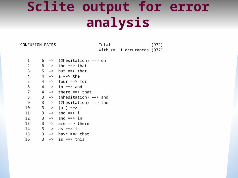
Sclite output for error analysis

CONFUSION PAIRS Total (972) With >= 1 occurances (972)

1: 6 -> (%hesitation) ==> on 2: 6 -> the ==> that 3: 5 -> but ==> that 4: 4 -> a ==> the 5: 4 -> four ==> for 6: 4 -> in ==> and 7: 4 -> there ==> that 8: 3 -> (%hesitation) ==> and 9: 3 -> (%hesitation) ==> the 10: 3 -> (a-) ==> i 11: 3 -> and ==> i 12: 3 -> and ==> in 13: 3 -> are ==> there 14: 3 -> as ==> is 15: 3 -> have ==> that 16: 3 -> is ==> this

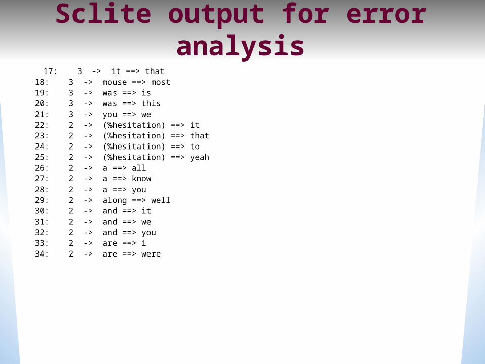
Sclite output for error analysis

17: 3 -> it ==> that 18: 3 -> mouse ==> most 19: 3 -> was ==> is 20: 3 -> was ==> this 21: 3 -> you ==> we 22: 2 -> (%hesitation) ==> it 23: 2 -> (%hesitation) ==> that 24: 2 -> (%hesitation) ==> to 25: 2 -> (%hesitation) ==> yeah 26: 2 -> a ==> all 27: 2 -> a ==> know 28: 2 -> a ==> you 29: 2 -> along ==> well 30: 2 -> and ==> it 31: 2 -> and ==> we 32: 2 -> and ==> you 33: 2 -> are ==> i 34: 2 -> are ==> were

Better metrics than WER?• WER has been useful• But should we be more concerned with meaning (“semantic error rate”)? Good idea, but hard to agree on Has been applied in dialogue systems, where desired semantic output is more clear

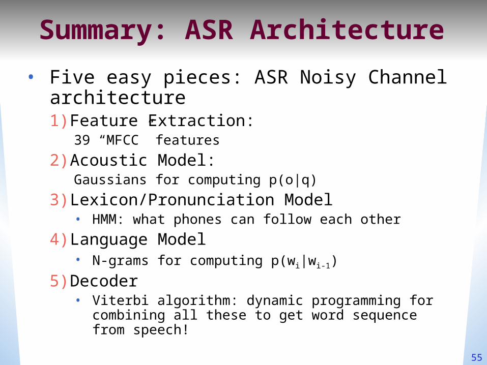
Summary: ASR Architecture• Five easy pieces: ASR Noisy Channel

architecture1)Feature Extraction:

39 “MFCC” features2)Acoustic Model:

Gaussians for computing p(o|q)3)Lexicon/Pronunciation Model

• HMM: what phones can follow each other4)Language Model

• N-grams for computing p(wi|wi-1)5)Decoder

• Viterbi algorithm: dynamic programming for combining all these to get word sequence from speech!

55

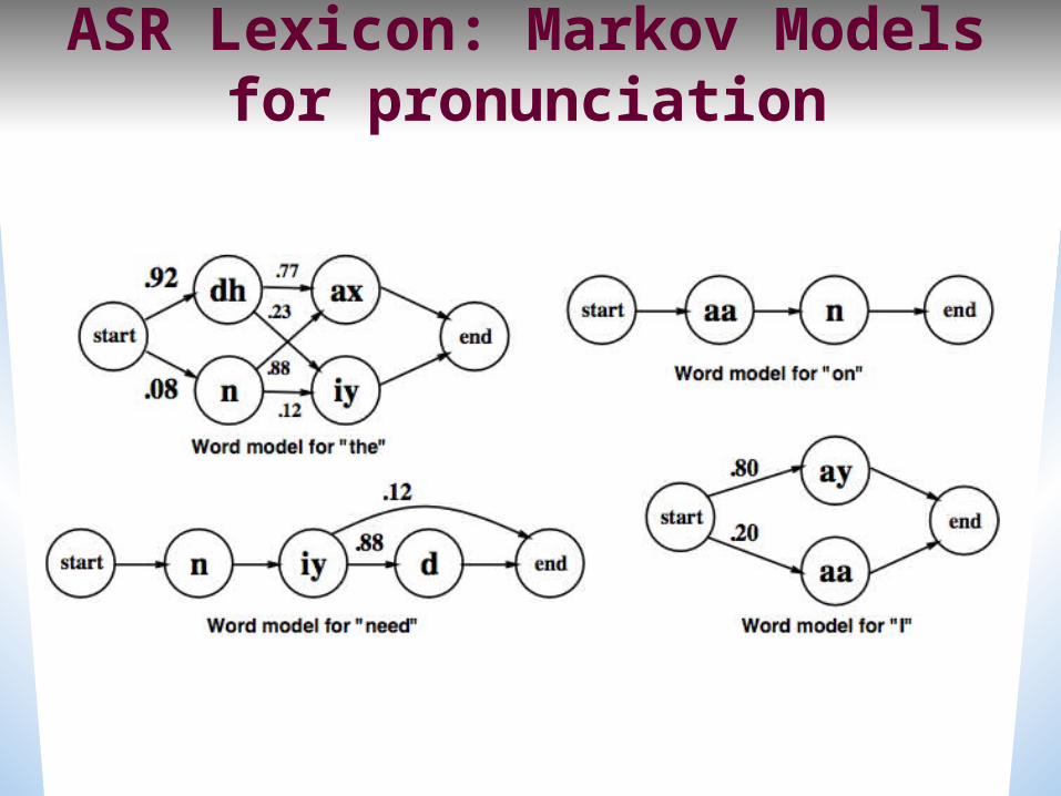
ASR Lexicon: Markov Models for pronunciation

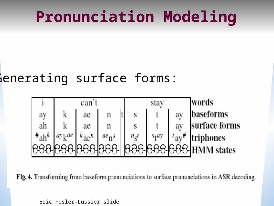
Pronunciation Modeling

Generating surface forms:

Eric Fosler-Lussier slide

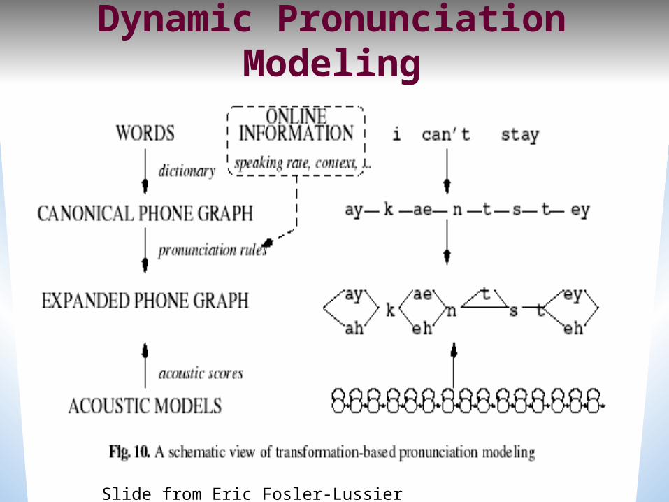
Dynamic Pronunciation Modeling

Slide from Eric Fosler-Lussier

Summary• Speech Recognition Architectural Overview

• Hidden Markov Models in general Forward Viterbi Decoding

• Hidden Markov models for Speech• Evaluation

Documents

Gaussian Mixture Model