On Factors of Non-singular Cartesian Products ∗

Andres del Junco † Cesar E. Silva ‡

January 3, 2000; August 30,2002

Abstract

We classify all factors of the Cartesian product of any two non-singular

type IIIλ, 0 < λ ≤ 1, or type II1 Chacon transformations, as well as the

centralizer of finite Cartesian products of such transformations.

1 Introduction

In [R79], Rudolph introduced the property of minimal self-joinings (MSJ) for finite

measure-preserving transformations; this is a strong property that led to a series

of important examples. In particular, this property implies that the factors of

Cartesian products of T with itself are just the obvious ones (those obtained by

fixing a co-ordinate and the symmetric factors). Rudolph also constructed examples

of mixing finite measure-preserving transformations satisfying the MSJ property

using an extension the “random spacers” method of Ornstein [O72]. Later it was

shown by the first author, Rahe, and Swanson [JRS80] that the much simpler weak

mixing (finite measure-preserving) Chacon transformation has the MSJ property.

This transformation has in turn been used as a source of many examples in ergodic

theory.

Rudolph and the second author in [RS89] generalized the notion of minimal self-

joinings to non-singular transformations, and constructed examples of non-singular

transformations, both with no equivalent σ-finite invariant measure and with equiva-

lent infinite σ-finite invariant measure, with the (non-singular) MSJ property. How-

ever, while the MSJ theory in Rudolph [R79] considers n-fold (measure-preserving)

∗2000 Mathematics Subject Classification. Primary 37A40. Secondary 28D. Key words and

phrases: ergodic, non-singular coding, factors, Cartesian product, non-singular Chacon maps.†Department of Mathematics, University of Toronto, Toronto M5S 1A1, CANADA‡Department of Mathematics,Williams College, Williamstown, MA 01267

1

self-joinigs of T , the non-singular theory in [RS89] was generalized only to 2-fold

self-joinings. The reasons for this were technical problems with extending the notion

of rational joinings from 2-fold to n-fold self-joinings. (It is shown in [RS89] that

the class of all non-singular joinings is too broad and that one must restrict them to

a subclass such as the rational joinings.) However, while the 2-fold (non-singular)

MSJ property is sufficient to imply primeness (i.e., no non-trivial invertible factors)

and trivial centralizer (i.e., commuting only with its powers) [RS89], it is not clear

whether it implies anything about the factors or centralizer of T ×T . In fact, a pri-

ori it seems that one needs to know the 4-fold joinings of T to control the factors of

T ×T , and it is an open problem even in the finite measure-preserving case whether

2-fold MSJ implies n-fold MSJ. We also note that while finite measure-preserving

odometers have uncountable centralizers, non-singular type IIIλ odometers with

trivial centralizer were constructed by Hamachi [H81] and later and independently

by Aaronson [Aa87] (see also [Aa97]). However these maps have non-ergodic Carte-

sian squares and non-trivial factors, and the methods of proof are different from

ours and the MSJ theory.

In this paper we approach the study of factors and centralizers of Cartesian prod-

ucts of non-singular transformations using coding techniques. Coding techniques

were used by the first author in [J78] to show that the classic Chacon automorphism

is prime and has trivial centralizer. Non-singular coding was later introduced by

the authors in [JS95], where it was used to show that the type IIIλ, 0 < λ < 1,

non-singular Chacon automorphisms are prime, and where many of the results of

this paper were announced. Here we extend our methods to study the centralizer

and factors for Cartesian products of these maps.

The paper is organized as follows. Section 2 starts with some preliminary defini-

tions and a self-contained presentation of non-singular codes. In section 3 we define

the non-singular Chacon maps. We start with the geometric definition of a map

Tλ, 0 < λ ≤ 1, on the unit interval with Lebesgue measure µ; we then show that

(Tλ, µ) is isomorphic to (T, µλ), where T is the shift on a symbolic space and µλ

is a non-singular Borel measure on this symbolic space. In our proofs we use the

symbolic version (T, µλ) but sometimes we refer to some properties that are easier

to see in the geometric version (Tλ, µ). Furthermore, to simplify notation, in some

cases we may write Tλ for the symbolic version (T, µλ). For each 0 < λ < 1, Tλ is

a type IIIλ non-singular map, and for λ = 1 it is the classical type II1 map. We

also show how to obtain type III1 Chacon maps for which our proofs also apply (see

2

Remark 1).

In section 4 we classify the centralizer of any finite Cartesian product of non-

singular Chacon maps and prove the following theorem.

Theorem A. (cf. Theorem 3 ) Let 0 < λ1 < . . . < λk ≤ 1 and n1, . . . , nk

be integers. Then the centralizer of the Cartesian product T⊗n1

λ1× . . . × T⊗nk

λkis

generated by maps of the form U1 × . . . × Uk, where each Ui, acting on the ni-

dimensional product space Xni , is a Cartesian product of powers of Tλi, or a co-

ordinate permutation on Xni .

Finally, in section 5 we prove the following theorem that classifies of all the

factors of the Cartesian product of any two non-singular type IIIλ, 0 < λ ≤ 1, or

type II1 Chacon maps.

Theorem B. (cf. Theorem 6) Let X = (X,B, µλ1, T ) and X = (X,B, µλ2

, T ) be

two non-singular Chacon systems. Let F be a factor algebra of (T × T, µλ1× µλ2

).

(a) If λ1 6= λ2 then F is equal modµ to one of the four algebras B ⊗ C, B ⊗ N ,

N ⊗ C, or N ⊗N (where N is the trivial algebra).

(b)If λ1 = λ2 then F is equal modµ to one of the following algebras B⊗C, B⊗N ,

N ⊗ C, N ⊗N , or (Tm × Id)B2⊙ for some integer m.

While in the finite measure-preserving case our results are not new, as they

follow from the MSJ property of Chacon’s map, our proofs are new also in the finite

measure-preserving case and provide another approach to controlling the centralizer

and factors of Cartesian products, independent of the MSJ theory. The reader

interested in our proof for the finite measure-preserving case may assume that our

d-distance is the classic one and that the Radon-Nikodym derivative (defined below)

is always 1.

Lastly, we mention a partial answer to a question in [CEP89], where Choksi,

Eigen and Prasad asked whether there exists a zero entropy, finite measure-preserving

mixing automorphism S, and a non-singular type III automorphism T , such that

T ×S has no Bernoulli factors. This question motivated in part the work in [RS89],

but the original question remained open. It follows from Theorem 1 that if S is the

finite measure-preserving mildly mixing Chacon automorphism and T is any non-

singular Chacon automorphism as defined here, the factors of T × S are only the

trivial ones, and so T ×S has no Bernoulli factors, partially answering the question

in [CEP89] with S mildly mixing instead of mixing.

3

Acknowledgments. The first author was supported in part by an NSERC grant.

The second author was supported in part by an NSF grant, and would like to thank

the University of Toronto for supporting a visit when this research began. We would

like to thank the referee for comments that improved the exposition.

2 Preliminaries

2.1 Non-singular Transformations

All the spaces we consider are standard (Borel) probability spaces, i.e., they consist

of a standard Borel space (X,B) and a probability measure µ on B. A set is co-null

if it is Borel and its complement is of measure 0. A map T : (X,B, µ) → (X,B, µ)

is a non-singular automorphism if there exists a co-null set X ′ ⊂ X such that

T : X ′ → X ′ is 1 : 1 and measurable, and for every A ∈ B ∩ X ′, µ(T−1A) = 0

if and only if µ(A) = 0. If T is as above but not necessarily 1 : 1 then it is

a non-singular endomorphism. A non-singular (dynamical) system consists of a

non-singular automorphism T defined on a standard space (X,B, µ); we sometimes

denote such a non-singular system by X = (X,B, µ, T ). T is ergodic if whenever

T−1(A) = A then µ(A)µ(Ac) = 0, and it is conservative if for all sets of positive

measure A there exists an integer n > 0 such that µ(T−n(A) ∩A) > 0. We denote

by C(X) or C(T ) the centralizer of T , that is, all non-singular endomorphisms S of

(X,B, µ) such that ST = T S a.e. We denote by F (X) the class of factor algebras

F of T , that is F is a sub-σ-algebra of B invariant under T : TF = F (modµ). Let

N , or N (X) denote the trivial sub-σ-algebra.

If X = (X,B, µ, T ) is a non-singular system we denote by ωi the Jacobian or

Radon-Nikodym derivative of T i:

µ(T iA) =

∫

A

ωidµ ∀A ∈ B. (2.1)

When µ or T i needs to be emphasized we write ωµ,T i . One has the cocycle relation

ωi(x)ωj(Tix) = ωi+j(x) a.e. (2.2)

If X = (X,B, µ, T ) is non-singular system, a factor of X is a non-singular sys-

tem Y = (Y, C, ν, S) such that there exist co-null sets X ′ ⊂ X,Y ′ ⊂ Y with

TX ′ ⊂ X ′, SY ′ ⊂ Y ′ and a measurable, measure-preserving φ : X ′ → Y ′, called

a homomorphism (or factor map), with φ T = S φ on X ′. (If φ is only non-

singular, by replacing ν with the equivalent measure µ φ−1 we can assume φ is

4

measure-preserving.) Clearly if φ is a homomorphism φ−1(C) is a factor algebra.

Furthermore, if F is a factor algebra of X then there is a non-singular system Y

and a homomorphism φ : X → Y such that F = φ−1C modµ, see e.g. [Aa97,

1.0.10]. We call φ the homomorphism corresponding to the factor algebra F .

If φ : X → Y is a homomorphism, µ may be disintegrated with respect to φ,

i.e., there exist a co-null set Y0 and a measurable map y → µy so that for all y ∈ Y0,

µy is a probability measure supported on φ−1y and such that

µ =

∫µydν(y). (2.3)

Furthermore, for all y = φ(x) ∈ Y0, µSy T is a measure equivalent to µy and

ωµ,T (x) = ων,S(y)dµSy T

dµy

(x) µy-a.e. for all y ∈ Y0. (2.4)

See e.g. [Aa97, 1.0.8, 1.0.11] or [RS89, 1.3.2]. One easily checks that

ων,S(y) =

∫

X

ωµ,T (x)dµy(x), for ν a.a. y. (2.5)

As is well-known, all finite measure-preserving (and all infinite measure-preserving)

automorphisms are orbit equivalent [D59,63]. The situation is quite different for

non-singular automorphisms. Krieger introduced in [Kr70] the ratio set as an in-

variant for orbit equivalence of nonsingular automorphisms and showed that all

type IIIλ, 0 < λ < 1, (defined below), and all type III1 automorphisms are orbit

equivalent [Kr76]. Given a non-singular automorphism T on (X,µ), the ratio set

of T , denoted by r(T ), is defined to be the set of non-negative real numbers t such

that for all ε > 0 and all measurable sets A of positive measure there exists n > 0

such that

µ(A ∩ T−nA ∩ x: ωT n(x) ∈ Nε(t)) > 0,

where Nε(t) = s ≥ 0 : |s− t| < ε.

The set r(T ) \ 0 is a closed multiplicative subgroup of the reals and if 0 ∈

r(T ) then T admits no equivalent σ-finite invariant measure. This allows four

possibilities: 1) r(T ) = 1, 2) r(T ) = 0, 1, 3) r(T ) = 0 ∪ λk : 0 < λ < 1, k ∈

Z., 4) r(T ) = [0,∞).

The first case is called type II and these are actions that admit an equivalent

σ-finite invariant measure; if the invariant measure is infinite we say it is type

II∞, otherwise it is type II1. The others are types III0, IIIλ, 0 < λ < 1, and

III1, respectively. For background material we refer to [Kr70],[Kr76], [HO81] and

[KW91].

5

2.2 Relative Product Measure

We use the relative product measure to study the factors of a non-singular sys-

tem. The relative product, introduced by Furstenberg for finite measure-preserving

systems and used in [RS89] in the nonsingular setting, is an example of a joining.

Although the only joining we will use is the relative product, we state several of the

results below in terms of joinings as that is their natural context.

If Xj = (Xj ,Bj , µj , Tj), j = 1, 2 are dynamical systems a (non-singular) joining

of X1 and X2 is a measure µ on B1×B2 projecting onto µ1 and µ2 and non-singular

for T1 × T2. We write

ω1i = ωµ1,T i

1

, ω2i = ωµ2,T i

2

, ωi = ωµ,T i1×T i

2

(2.6)

for i ∈ Z. As a special case of (2.5) on has

ω1i (x1) =

∫

X2

ωi(x1, x2)dµx1(x2) (2.7)

where µ =∫

X1

µx1dµ1(x1) is the disintegration of µ over the first co-ordinate in

X1 × X2. Following [RS89], µ is called a rational joining if there are measurable

functions c1(x1) and c2(x2) such that

ω(x1, x2) = ω1(x1)ω2(x2)c

1(x1) = ω1(x1)ω2(x2)c

2(x2) µ a.e. (2.8)

Our main use of rational joinings is that the relative product joining is rational as

we see below. However, without the need to change any of the arguments, the reader

who wishes to may substitute “rational joining” with “relative product joining” in

Lemma 2.1 (assuming X1 = X2) and Corollary 3.2.

If φ : X → Y is a homomorphism, the relative product measure µ = µ×φ µ on

X ×X is defined by

µ =

∫µy × µydν(y), (2.9)

where µ =∫µydν(y) is the disintegration of µ over Y.

It is straight forward to check that the relative product µ is a non-singular

joining of X with X. To see that is is rational note that

ω(x1, x2) =ω1(x1)ω

2(x2)

ων,S(φ(x1))=

ω1(x1)ω2(x2)

ων,S(φ(x2)), (2.10)

where ω1 = ω2 = ωµ,T . Since µ is supported on (x1, x2) : φ(x1) = φ(x2), then

φ(x1) = φ(x2) µ a.e. If we let c1(x1) = 1ων,S(φ(x1))

and c2(x2) = 1ων,S(φ(x2))

then

formula (2.8) is satisfied and so the relative product is a rational joining.

6

The following lemma, implicit in [RS89] (Proposition 4.3.2), plays an important

role for our arguments as it is used to bound the Radon-Nikodym derivatives of the

relative products. Though we use it only for the relative product, it is stated in its

natural context of rational joinings.

Lemma 2.1. ([RS89]) Suppose that µ is a rational joining of X1 and X2, i ∈ Z,

and there exists a constant C ∈ (0, 1) such that

C < ωji < C−1 µj-a.e. j = 1, 2 .

Then

C3 < ωi < C−3 µ-a.e.

Proof. Apply the cocycle relation (2.2) to (2.8) to obtain

ωi(x1, x2) = ω1i (x1)ω

2i (x2)c

1i (x1) µ−a.e., (2.11)

where c1i (x) = c1(x) · · · c1(T i−11 (x)), i ≥ 1. Let µ =

∫µx1

dµ1(x1) be the disin-

tegration of µ over X1. Integrating (2.11) with respect to µx1we get for µ1-a.a.

x1

ω1i (x1) = ω1

i (x1)ci(x1)

∫ω2

i (x2)dµx1(x2)

so

C < ci(x1) =

( ∫

X2

ω2i (x2)dµx1

(x2)

)−1

< C−1 ,

since for µ1-a.a. x1, C < ω2i (x2) < C−1 for µx1

-a.a. x2. Substitute this inequality

back into (2.11) to complete the proof.

2.3 Non-singular Codes

We now give a self-contained presentation of the main properties of the non-singular

d-distance introduced in [JS95]. Denote intervals in Z by [m,n] = m,m+1, . . . , n.

Let Z = (Z,D, λ, R) be any non-singular system and z ∈ Z. Let Ωλ,z denote the

measure on Z defined by Ωλ,z(i) = ωλ,Ri(z). We sometimes write Ωz instead of

Ωλ,z when λ is clear from the context. Given sequences ξ, η ∈ AZ, A finite, let

D(ξ, η) = i : ξ(i) 6= η(i).

For I ⊂ Z, I finite, define

dIz(ξ, η) = Ωz

(D(ξ, η) ∩ I

)/Ωz(I)

7

and then let

dz(ξ, η) = limm,n→∞

d[−m,n]z (ξ, η) ,

if the limit exists; equivalently

dz(ξ, η) = limm→∞

d[−m,0]z (ξ, η) = lim

n→∞d[0,n]

z (ξ, η)

if the two limits exist and agree. When we want to emphasize the measure λ we

will write dz = dz,λ. It is clear that dz satisfies the triangle inequality.

For any interval I let σ(I) denote the smallest symmetric interval containing I.

Lemma 2.2. Suppose dz(ξ, η) exists. Let I1, I2, . . . be a sequence of intervals in Z

with⋃∞

n=1 σ(In) = Z and such that there is a constant C′ with

Ωz

(σ(In)

)≤ C′Ωz(In) for all integers n.

If limn→∞ dInz (ξ, η) = 0 then dz(ξ, η) = 0.

Proof. This is just a fact about measures on Z. The hypothesis implies that if d is

small on In then it is small on σ(In), and so it is 0 on Z since its value on Z is the

limit of its values on σ(In).

Y = (Y, C, ν, S) is called a (non-singular) symbolic system, with alphabet A, if

Y = AZ, A is finite, C is the Borel σ-algebra on Y, S is the left shift on Y and ν is any

measure non-singular for the shift map. If x ∈ AZ (i.e. x : Z → A) and I = [m,n]

we denote the restriction x |I by x[m,n] ∈ AI . When it is clear from the context

we will sometimes identify AI with Am−n+1, i.e., we think of x[m,n] as a word of

length m − n + 1 with no particular indexing. By a code ψ : AZ → BZ, A and B

finite, we mean any measurable shift-commuting map. A finite code ψ : AZ → BZ

is a map ψ = ψf , determined by the choice of a funtion f : A2k+1 → B, for some

k, via the formula

ψf (x)(i) = f(x[i− k, i+ k]

).

Such a ψ automatically commutes with the shifts. 2k + 1 is called the code length

of ψ, and denoted |ψ|. If ψ and ψ′ are any two codes from AZ to BZ we define

D[ψ, ψ′] = x ∈ AZ|ψ(x)(0) 6= ψ′(x)(0).

(Note that D(ξ, η) is used for the set of indexes where two sequences differ, while

D[ψ, ψ′] is the set of points in AZ where the codes differ at the 0th place.)

Lemma 2.3. Suppose (AZ, µ) is a non-singular symbolic system and φ, φ′ : AZ →

BZ are any two codes. Then for almost all x ∈ X dx(φ(x), φ′(x)) exists.

8

Proof. Apply the Hurewicz ergodic theorem to the set D[φ, φ′] (in way a similar to

the proof of Proposition 2.4).

A homomorphism φ between non-singular symbolic systems (AZ, µ) and (BZ, ν)

can be approximated by a finite code by approximating the setsx : φ(x)(0) = b

,

b ∈ B, by cylinders of length 2k + 1 in AZ to obtain f : A2k+1 → B and hence a

finite code φ′ = ψf . More precisely, we require D[φ, φ′] to have small µ-measure.

(It is important to be aware that φ′ will not be a homomorphism from (AZ, µ) to

(BZ, ν) since it will not be non-singular.) An application of the ergodic theorem

then leads to the following d-bar approximation.

Proposition 2.4. ([JS95]) Let X and Y be non-singular symbolic systems with

alphabets A and B, φ : X → Y a homomorphism and φ′ a finite code such that

µ(D[φ, φ′]) < ǫ2, 0 < ǫ < 1. Suppose X′ is a third non-singular symbolic system

and λ is any conservative joining of X and X′. Then

λz = (x, x′) ∈ X ×X ′|dz(φ(x), φ′(x)) < ǫ > 1 − ǫ.

Here dz = dz,λ.

Proof. Let Eλ(h|I) denote the conditional expectation of h with respect to the

algebra of invariant sets I in X × X′. Using the fact that φ and φ′ commute with

the shifts one sees that for x ∈ X

i : T ix ∈ D[φ, φ′]

= D

(φ(x), φ′(x′)

). (2.12)

Let D = D[φ, φ′]. Apply the Hurewicz ergodic theorem to T × T ′, λ to get

Eλ(1D×X′ |I)(x, x′) = limn→∞

n∑i=0

ωi(x, x′)1D×X′(T ix, T ′ix′)

n∑i=0

ωi(x, x′)(2.13)

= limn→∞

Ω(x,x′)

(i : T ix ∈ D ∩ [0, n]

)

Ω(x,x′)[0, n](2.14)

= limn→∞

d[0,n](x,x′)(φ(x), φ′(x)) . (2.15)

Since the invariant σ-algebra of T−1 × T ′−1is the same as that of T × T ′ we

also get

Eλ(1D×X′ |I)(x, x′) = limn→∞

d[−n,0](x,x′) (φ(x), φ′(x)) .

The integral of the expectation is the same as the integral of 1D×X′ which is

µ(D[φ, φ′]), since λ is a joining. By Chebyshev’s inequality,

λz|dz(φ(x), φ′(x)) ≥ ǫ ≤1

ǫ

∫dz(φ(x), φ′(x))dλ =

1

ǫµ(D[φ, φ′]) < ǫ,

9

which completes the proof.

The following proposition is standard in the measure-preserving case, but we

need it in the more general form below.

Proposition 2.5. ([JS95]) Let X = (X,B, µ, T ) be a (not necessarily ergodic)

non-singular system and let F be a factor algebra which is ergodic, i.e., TA = A,

A ∈ F ⇒ µ(A) = 0 or 1. Let I denote the σ-algebra of T -invariant sets. Suppose

that h is a F-measurable function such that h ≥ 0 and µE(h | I) = 0

> 0. Then

h = 0 a.e.

Proof. We use the following property of the ergodic decomposition of µ: there is

a homomorphism φ : X → Y = (Y, C, ν, id) such that φ−1(C) = I and if µ =∫µydν(y) is the disintegration of µ over Y then for ν-a.e. y µy is non-singular and

ergodic for T .

Let E = y :∫

Xhdµy = 0. Our hypothesis is that ν(E) > 0, and we need to

show that ν(E) = 1. Define the measure

µ =

∫

E

µydν(y)

and let µF and µF denote the restrictions to F . Then µF is absolutely continuous

with respect to µF , and by ergodicity of µF it follows that µF is equivalent to µF .

The definition of µ implies that h = 0 µF -a.e., so h = 0 µF -a.e., which completes

the proof as h is F -measurable.

3 Non-singular Chacon maps

3.1 Geometric Construction

In this section we recall the definition of non-singular Chacon maps [JS95]. We

first describe them geometrically as rank one cutting and stacking constructions,

and then use a natural partition to code them to symbolic systems with alphabet

0, 1. We fix a λ ∈ (0, 1]. When λ = 1 the construction yields the classical finite

measure-preserving Chacon map. When 0 < λ < 1 it yields a type IIIλ non-singular

map. We describe later how to obtain a type III1 map.

To start the construction let

α =1 + λ

1 + 2λ,

10

and let I0 = [0, α). Partition I0 into the contiguous intervals J01 , J

02 and J0

4 of

lengths λ1+2λ

α, 11+2λ

α, and λ1+2λ

α; i.e., their lengths are in the proportion λ, 1, λ.

Then let J03 be an interval of length 1

1+2λα abutting on I0. Define Tλ : J0

i → J0i+1

for i = 1, 2, 3 to be the affine map that takes J0i to J0

i+1, and leave Tλ undefined

on J4. This produces a column or tower ξ1 for Tλ of height 4 whose levels are

intervals; Tλ has constant Radon-Nikodym derivatives on each level, except the top

one, where Tλ is not yet defined. The union of the levels is a new interval I1.

Assume by induction that at stage n of the construction we have a column ξn

of height hn whose levels are intervals with union In, also an interval, and Tλ is

an affine map on each level to the one above, and as yet is undefined on the top

level. We extend the definition of Tλ as follows. Partition the base (i.e., lowest level)

B(ξn) of column ξn into intervals Jn1 , J

n2 , J

n4 of lengths proportional to λ, 1, λ, and

let Jn3 be an interval of the same length as Jn

2 abutting on In. Extend Tλ affinely

so that

Tλ : T hn−1λ Jn

1 → Jn2 ,

Tλ : T hn−1λ Jn

2 → Jn3 ,

Tλ : Jn3 → Jn

4 ,

to obtain a column ξn+1 of height hn+1 = 3hn + 1. We note that ωµ,Tλ= λ−1 on

T hn−1λ Jn

1 , ωµ,Tλ= 1 on T hn−1

λ Jn2 and ωµ,Tλ

= λ on Jn3 = T hn

λ Jn2 .

We have constructed a sequence of columns ξn on intervals In, and one can verify

that In ↑ [0, 1), Tλ is defined a.e. on X = [0, 1) and is a non-singular automorphism

with respect to Lebesgue measure µ on X , with B the Borel σ-algebra of X .

To obtain a type III1 example choose 0 < λ1 < λ2 < 1 such that log(λ1)/ log(λ2)

is irrational and in the construction of the columns ξn, for n even divide B(ξn) in

the ratio a, b, a with a/b = λ1, and for n odd in the ratio a, b, a with a/b = λ2;

denote this transformation by Tλ1,λ2.

The construction of type II∞ and type III0 nonsingular Chacon transformations

is more complex as it needs the choice of λ to vary with n in a controlled way.

This has been done recently in [HS00] (written after the first version of this paper);

however the only property proved for these maps in [HS00] is ergodicity of their

2-fold Cartesian product. In [HS00], at stage n in the construction, the levels of ξn

are divided in the rations a, b, a with a/b = λn, and in the type III0 and type II∞

cases the choice of the λn is such the the bounds in Proposition 3.1 do not hold.

11

As explained later (cf. Remark 1) the bounds of Corollary 3.2, which follow from

Proposition 3.1, are crucial to our arguments.

In this section we obtain some estimates about the Radon-Nikodym derivatives

of joinings of products of non-singular Chacon maps. These estimates are possi-

ble along the column heights, and are based on the following proposition whose

proof is contained in the proof of [JS95], Proposition 3.1. We include the proof for

completeness.

Proposition 3.1. ([JS95]) Let X = (X,B, µ, Tλ) be a non-singular Chacon system.

Then

1. λ ≤ ωµ,Tλ≤ λ−1 µ a.e.

2. ∀n, λ2 ≤ ωµ,T

hnλ

≤ λ−2 µ a.e.

Proof. Let ω = ωµ,Tλ. Clearly, ω(x) ∈ λ−1, 1, λ a.e. Note that if ωhn

is constant

on an interval I, then for all x ∈ I, ωhn(x) = µ(T hn (I))

µ(I) . Let J be any level of

column ξn and let J(1), J(2), J(3) denote the three subintervals that J is divided into

when constructing the levels of ξn+1. Since ω is constant on levels of ξn, by the

cocycle relation, ωhnis constant on J(1) and on J(2). Also, it is constant on the first

and second thirds of J(3), and so on. It follows that if x ∈ ξn, then ωhn(x) = λ−1

or ωhn+1(x) = λ (according to whether or not T i(x) is in ξn for i = 0, . . . , hn). If x

is not in any level of ξn then ωhn+1(x) = λ or ωhn+1(x) = 1. (The last possibility

occurs only when x lies in Jn3 [the interval added at the nth stage of the construction]

and T hn+1x ∈ B(ξn).) The cocycle relation implies that λ+2 ≤ ωhn(x) ≤ λ−2.

The following is now a consequence of rationality and Proposition 3.1.

Corollary 3.2. Let X = (X,B, µλ1, T ) and X = (X,B, µλ2

, T ) be two non-singular

Chacon systems. Let m1,2 = µλ1×µλ2

and m be any rational joining of (T×T,m1,2)

and (T ×T,m1,2). Let T4 denote the transformation (T ×T )×(T ×T ) with measure

m1,2 ×m1,2. Let z ∈ (X ×X)× (X ×X) and write Ωz for the measure Ωm,z on Z

as defined earlier. Let Ωx denote the measure Ωλ1,x. Then

1. ∀n, (λ1λ2)6 ≤ ω

m,Thn4

≤ (λ1λ2)−6 m a.e., and so (T4, m) is conservative.

2. ∀k, (λ1λ2)3k ≤ ωm,T k

4

≤ (λ1λ2)−3k m a.e.

3. ∀C > 0 ∃C′ > 0 such that for m-a.a. z whenever I1 ⊂ I2 are intervals in

Z with |I2| < C|I1| then Ωz(I2) < C′Ωz(I1). The analogous statement also

holds for the measure Ωλ1,x.

12

4. ∀k ∈ Z+, ε > 0 ∃L > 0 such that for m-a.a. z whenever I1 ⊂ I2 are intervals

in Z with |I1| < k and |I2| > L then Ωz(I1) < εΩz(I2). The analogous

statement also holds for the measure Ωλ1,x.

5. ∀n > 0 and i ∈ Z, (λ1λ2)6 < Ωzi

/Ωzi+ hn < (λ1λ2)

−6. The analogous

statement also holds for the measure Ωλ1,x.

Proof. We first show part 1. Let T2 denote T × T with measure m1,2. Since

ωm1,2,T

hn2

(x1, x2) = ωµλ1,T hn (x1) ωµλ2

,T hn (x2),

using Proposition 3.1,

(λ1λ2)2 ≤ ω

m1,2,Thn2

≤ (λ1λ2)−2.

Now Lemma 2.1 completes the proof. Part 2 follows in a similar way (using the

cocycle relation instead of Proposition 3.1). For part 3, since for all n, hn+1/hn ≤ 4

there is an n such that hn ≤ |I1| ≤ 4hn. Let J ⊂ I1 be any interval of length hn.

Then I2 can be covered by at most 4C + 1 intervals J + ihn with |i| < 4C + 1. By

part 1 we get

Ω(x1,x2)(I2) ≤ C′Ω(x1,x2)(J) ≤ C′Ω(x1,x2)(I1)

with C′ = (4C + 1)(λ1λ2)−6(4C+1). The proof of the second part for the measure

Ωλ1,x is similar.

To prove part 4 we may assume k = 2 (i.e., |I1| = 1). Since hn ≤ 4n, using part

1 we obtain

4n∑

i=0

ωm,T i4

> n(λ1λ2)6 and

0∑

i=−4n

ωm,T i4

> n(λ1λ2)6 µ-a.e.

This means that Ωzj/Ωz[j, j + 4n] < 1

n(λ1λ2)

−6 and Ω(x1,x2)j/Ωz[j − 4n, j] <

1n(λ1λ2)

−6, so 4 follows. Part 5 is just a restatement of 1.

Proposition 3.3. For each 0 < λ < 1, the map Tλ is a non-singular conservative,

ergodic type IIIλ automorphism. For λ = 1, T1 is the classical finite measure-

preserving Chacon transformation. If log(λ1)/log(λ2) is irrational then Tλ1,λ2is a

conservative, ergodic type III1 automorphism.

Proof. Let T = Tλ. As before, let J(1), J(2), J(3) denote the three subintervals that

a level J in column ξn is divided into when constructing the levels of column ξn+1.

13

As the levels in ξn∞n=0 generate, for any sets A,B of positive measure there exist

levels J and K in some column ξn so that for each k = 1, 2, 3,

µ(J(k) ∩A) >1

2µ(J(k)) and µ(K(k) ∩B) >

1

2µ(K(k)).

It is clear then that there is an integer ℓ > 0 such that µ(T ℓ(A) ∩ B) > 0, so T is

conservative ergodic. Also, T hn(J(1)) = J(2) and ωT hn = 1/λ on J(1). Therefore, for

every ε > 0, µ(A ∩ T−hn(A) ∩ x : ωT hn (x) ∈ N(1/λ, ε)) > 0 and so 1/λ ∈ r(T ).

Since ωT i takes only values that are powers of λ it follows that T is type IIIλ.

In the case of Tλ1,λ2a similar argument shows that λ1, λ2 ∈ r(Tλ1,λ2

), and since

r(Tλ1,λ2) \ 0 is a closed multiplicative subgroup the hypothesis implies that the

ratio set is [0,∞).

We now state two theorems about nonsingular Chacon maps that we use. The-

orem 1 was proved in [JS95], however section 5 contains all the ideas needed for its

proof.

Theorem 1. ([JS95]) Let X = (X,B, µ, Tλ) a non-singular Chacon system. Let

F be a factor algebra of T . Then T is prime, i.e., F is equal modµ to the full

σ-algebra B or the trivial σ-algebra N .

Using the techniques of this paper the authors have shown that T ×T is ergodic

(unpublished). We will use the stronger property below (Theorem 2) that was

shown in [AFS01] by different methods.

Theorem 2. ([AFS01]) Let 0 < λ1 ≤ . . . ≤ λk ≤ 1 and n1, . . . , nk be nonzero

integers. Then T n1

λ1× . . .× T nk

λkis ergodic.

3.2 Symbolic Chacon Maps

We now describe the symbolic version of Tλ. Let P be the two-set partition which,

viewed as function into 0, 1, is defined by

P (x) =

0, if x ∈ I0,

1, if x ∈ X − I0.

For x ∈ X let θ(x) ∈ 0, 1Z denote the “ P, Tλ-name” of x:

θ(x)(i) = P (T iλx) .

Define blocks of 0’s and 1’s inductively as follows:

B0 = 0, B1 = 0010, Bn+1 = BnBn1Bn .

14

Clearly Bn is the partial P, Tλ-name θ(x)[0, hn − 1] of any point in the base of ξn.

One can show that the cutting and stacking construction we have described is

isomorphic via θ to a symbolic system with alphabet 0, 1 which we shall denote

by X = (X,B, µλ, T ); here T is always the shift, µλ = µ θ−1, and for λ1 6= λ2 the

measures µλ1and µλ2

are mutually singular. We end with the following proposition,

whose proof can be found in [JS95], about the symbolic structure of the Chancon

maps.

Proposition 3.4. (cf. [JS95]) For each λ ∈ (0, 1] there is a Borel subset Xλ ⊂ X

such that µ(Xλ) = 1 with the following properties:

(a) For each n, x ∈ Xλ decomposes uniquely as a concatenation of n-blocks Bn,

some of which are separated by a single 1. Let us call such 1’s in x (n-block) spacers.

Any appearance of Bn in x must be one of the Bn’s in the unique decomposition.

(b) For all x ∈ Xλ and for all sufficiently large n = n(x) the 0th co-ordinate in x

lies inside an n-block, which we call the time 0 n-block. The union over n of the

intervals on which the time 0 n-blocks occur is Z.

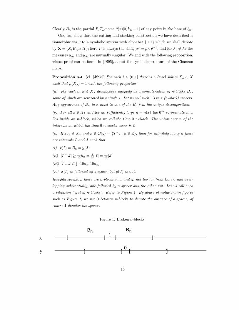
(c) If x, y ∈ Xλ and x 6∈ O(y) = T ny : n ∈ Z, then for infinitely many n there

are intervals I and J such that

(i) x(I) = Bn = y(J)

(ii) |I ∩ J | ≥ 110hn = 1

10 |I| = 110 |J |

(iii) I ∪ J ⊂ [−10hn, 10hn]

(iv) x(I) is followed by a spacer but y(J) is not.

Roughly speaking, there are n-blocks in x and y, not too far from time 0 and over-

lapping substantially, one followed by a spacer and the other not. Let us call such

a situation “broken n-blocks”. Refer to Figure 1. By abuse of notation, in figures

such as Figure 1, we use 0 between n-blocks to denote the absence of a spacer; of

course 1 denotes the spacer.

Figure 1: Broken n-blocks

x

y

Βn Βn1[ ] [ ]

[ ] [ ]0

15

Remark 1. We can think of (X,B, µλ, T ) as the topological Chacon map T with a

nonsingular, non-atomic, ergodic Borel measure µλ; µλ is obtained from the isomor-

phism θ with the geometric construction (X,B, µ, Tλ), where µ is Lebesgue measure

on the interval. For our arguments in sections 4 and 5 we will use the symbolic

version but properties of the measure that come from the geometric construction.

However, on close inspection of the proofs we see that the only properties that we

use, in addition to the name structure of the topological map, are the bounds on

the Radon-Nikodym derivatives in Proposition 3.1; once they are established Corol-

lary 3.2 follows. Thus we are able to prove our results for any non-singular, non-

atomic ergodic Borel probability measure for which the Radon-Nikodym derivatives

obey bounds such as in Proposition 3.1. In particular, while we discuss our proofs

in terms of type IIIλ measures, 0 < λ < 1, they also apply to the type III1 transfor-

mation Tλ1,λ2. (Theorem 2, as remarked in [AFS01], also holds for III1 transfor-

mations.)

4 The Centralizer of Products

Our main theorem in this section is the classification of the centralizer of Cartesian

products of non-singular Chacon maps (Theorem 3).

Remark 2. In this and the following sections (T, µλ) is always the symbolic rep-

resentation of the type IIIλ Chacon map, and T is the shift. To simplify notation

sometimes we write Tλ instead of (T, µλ), such as in the statement of Theorem 3.

We let T⊗nλ denote the n-fold Cartesian product of Tλ and let Xn denote the Carte-

sian product of n copies of X.

The following theorem classifies the centralizer of Cartesian products and is the

main result of this section.

Theorem 3. Let 0 < λ1 < . . . < λk ≤ 1 and n1, . . . , nk be integers. Then C(T⊗n1

λ1×

. . .× T⊗nk

λk) is generated by maps of the form U1 × . . . × Uk, where each Ui acting

on Xni is a Cartesian product of powers of Tλi, or a co-ordinate permutation on

Xni .

We start with a special case that will form the base case of the inductive proof

of Theorem 3.

Theorem 4. Any homomorphism from (T, µλ) to itself is a power of T . If λ1 6= λ2

then there is no homomorphism from (T, µλ1) to (T, µλ2

).

16

Proof. Suppose φ is a homomorphism from T to itself. The proof that φ is a

power of T is essentially the same as the by now classical argument [J78] that the

centralizer of the measure-preserving Chacon map is trivial, with some technical

modifications to deal with the weighted version of the d-distance. We will present

the proof informally.

Find a finite code φ′ of length k such that D[φ, φ′] has measure less than ǫ. Since

T is ergodic we have for a.a. x

dx(φ(x), φ′(x)) = µ(D[φ, φ′]) < ǫ. (4.1)

Moreover a.a. x will satisfy

dx(φ(x), T n(x)) = µ(D[φ, T n]), (4.2)

dx(φ(x), φT (x)) = µ(D[φ, φ T ]) (4.3)

and

both x and φ(x) lie in the set Xλ of Proposition 3.4. (4.4)

Fix x satisfying (4.1),(4.2), (4.3), (4.4) and suppose that y = φ(x) is not in the

orbit of x. Now choose n such that hn is much larger than k = |φ| and we see

broken n-blocks in (x, y). So, there are n-blocks in x and y occurring on intervals

I, J ⊂ [−10hn, 10hn] with |I∩J | > hn/10 and these n-blocks are followed by spacers

s1, s2 with s1 6= s2. (As explained earlier, “followed by a spacer s” means followed

or not followed by a spacer according as s is 1 or 0.) For concreteness we will

suppose s1 = 1 and s2 = 0.

Our goal now is to see that

dI∩Jx (y(I ∩ J), y((I ∩ J) + hn + 1)) is small . (4.5)

To see this we will be comparing sequences defined on I ∩ J , I ∩ J + hn and

I ∩ J + hn + 1. This will be justified by Corollary 3.2 (5) which guarantees that

each of the metrics dI∩Jx , d

(I∩J)+hnx , d

(I∩J)+hn+1x is bounded by a constant times any

other, independent of n. Thus, if α and β are any two sequences of length |I ∩ J |

we will simply write α ∼ β to mean that the sequences are close with respect to

one, and hence, all of these metrics.

First observe that since s1 = 1 we have x(I ∩ J) = x((I ∩ J) + hn + 1) so

φ′(x)(I ∩ J) ∼ φ′(x)((I ∩ J) + hn + 1), (4.6)

17

since these two sequences will agree except on the leftmost and rightmost k places.

When hn is sufficiently large these places contribute only a small amount to dx by

Corollary 3.2 (4). Next, if hn is sufficiently large φ′(x)[−10hn, 10hn] ∼ φ(x)[−10hn, 10hn]

by (4.2) and since |I ∩ J | > hn/10 it follows from Corollary 3.2 (3) that

φ′(x)(I ∩ J) ∼ φ(x)(I ∩ J). (4.7)

Similarly

φ′(x((I ∩ J) + hn + 1) ∼ φ(x((I ∩ J) + hn + 1). (4.8)

Combining (4.6), (4.7) and (4.8) gives (4.5).

Now observe that Ty(I ∩ J) = y((I ∩ J) + hn + 1), since s2 = 0. Thus (4.5)

becomes

dI∩Jx (y(I ∩ J), T y((I ∩ J))) is small .

Of course “is small” here means “< ǫ1” where ǫ1 goes to zero with ǫ. I = In and

J = Jn depend on n and n→ ∞ as ǫ→ 0. Since |In ∩ Jn| > hn/10, applying (4.3),

Lemma 2.2 and Corollary 3.2 (3) we can conclude that

dx(φ(x), T (φ(x)) = 0 = µ(D[φ, φ T ]).

From this it follows that φ = φ T , so, by ergodicity of T , φ is constant a.e., a

contradiction. This contradiction means that in fact y is in the orbit of x, that is

φ(x) = T n(x) for some n. By (4.2) it follows that φ = T n a.e.

Finally suppose that λ1 6= λ2 and φ is a homomorphism from (T, µλ1) to (T, µλ2

).

Since the measures µλ1and µλ2

are mutually singular they give full measure to

disjoint T -invariant sets. This means that we may assume as above that y = φ(x)

is not in the orbit of x and arrive at a contradiction as above.

The following lemma forms the basis of the inductive step that we shall need.

Lemma 4.1. If φ is any homomorphism from T⊗n1

λ1× . . . × T⊗nk

λkto Tλ with n =

n1 + . . . + nk > 1 then φ is a function of some strict subset of the co-ordinates of

x ∈ Xn1 × . . .×Xnk .

Proof. Let µn denote the product measure onXn, let δ denote the n-tuple (−1, 0, . . . , 0)

and let T δ = T−1×T 0×. . . T 0. Let φ′ be a finite code of length k with µn(D[φ, φ′]) <

ǫ. µn-a.a. x ∈ Xn will satisfy

dx(φx, φ′x) = µn(D[φ, φ′]) < ǫ, (4.9)

dx(φT δx, φx) = µnD[φ T δ, φ] and (4.10)

dx(φT δx, Tφx) = µnD[φ T δ, T φ]. (4.11)

18

Given x ∈ Xn let us saym > 0 is favorable if the following happens: there arem-

blocks in x1, . . . , xn occurring on intervals I1, . . . In such that Ij ⊂ [−10hm, 10hm],

|I1 ∩ . . . ∩ In| > hm/10 and I1 is followed by a spacer but the remaining Ij are not

followed by spacers. The Borel-Cantelli lemma ensures that for µn-a.a. x

there are infinitely many favorable m. (4.12)

Now fix an x satisfying (4.9), (4.10), (4.11) and (4.12) and choose a favorable m

with hm ≫ | φ′| = k. Let I1, . . . In be the intervals implied by the favorability of m

and let I = I1∩ . . .∩ In. The placement of spacers implies that T δx(I) = x(I+hm)

so it follows that

φ′(T δx)(I) = φ′(x)(I + hm), (4.13)

except for possibly the left and rightmost k indices. Now the left and right hand

sides of (4.13) are close to φ(T δx)(I) and φ(x)(I+hm) in the metrics dIx and dI+hm

T δx

respectively. As in the proof of Theorem 4 these two metrics are comparable to

each other so we conclude from (4.13) that

dx(φ(T δx)(I), φ(x)(I + hm)) is small. (4.14)

So far we have said nothing about the m-blocks and spacers in y = φ(x). In

fact all we need is the following simple observation: if y is any point in the set Xλ

defined in Proposition 3.4 and I is any interval of length greater than hm/10 then I

has a subinterval of length greater than hm/30 such that y(I + hm)(I ′) agrees with

either y(I ′) or T−1(y)(I ′). (If no spacer occurs in I we may take I = I ′, otherwise

we just take the part of I to the left or right of the spacer, whichever is largest.)

Applying this to y = φ(x) we get an I ′ ⊂ I such that φx(I ′ +hm) = T ǫφx(I ′) where

ǫ is either 0 or −1. If ǫ = 0 we conclude that φT δx(I ′) and φx(I ′) are close in dx

and then using (4.10) and arguing as in Theorem 4 we find that φ T δ = φ so φ

is a function of all but the first co-ordinate of x ∈ X . If ǫ = −1 we conclude that

φ(T δx)(I ′) and T−1φ(x)(I ′) are close in dI′

x , whence φ T δ = T−1 φ by (4.11).

This means that

φ = T φ T δ = φ (T × . . .× T ) T δ

= φ (Id× T⊗(n−1)).

Since T⊗(n−1) is ergodic it follows that φ depends only on the first co-ordinate of

x.

Now we are ready to prove the following theorem.

19

Theorem 5. If φ is a homomorphism from T⊗n1

λ1× . . .× T⊗nk

λkto Tλ then after a

co-ordinate permutation we must have λ = λ1 and φ is the projection onto the first

co-ordinate followed by a power of Tλ.

Proof. The proof is by induction using Theorem 4 and Lemma 4.1.

Now an easy argument shows that Theorem 3 above is a consequence of Theo-

rem 5. (In fact Theorem 5 can easily be used to characterize all homomorphisms

from T⊗n1

λ1× . . .× T⊗nk

λkto T

⊗n′

1

λ′

1

× . . .× T⊗n′

k′

λ′

k′

.)

5 Factors of Cartesian products

Let π denote the permutation on X ×X defined by π(x, y) = (y, x), and let B2⊙

denote the symmetric factor, i.e., B2⊙ = A ∈ B ⊗ B : π(A) = A. We now state

our main theorem.

Theorem 6. Let X = (X,B, µλ1, T ) and X = (X,B, µλ2

, T ) be two non-singular

Chacon systems. Let F be a factor algebra of (T × T, µλ1× µλ2

).

(a) If λ1 6= λ2 then F is equal modµ to one of the four algebras B ⊗ C, B ⊗ N ,

N ⊗ C, or N ⊗N .

(b)If λ1 = λ2 then F is equal modµ to one of the following algebras B⊗C, B⊗N ,

N ⊗ C, N ⊗N , or (Tm × Id)B2⊙ for some integer m.

The proof will proceed via several lemmas. Let us agree to refer to the factors

specified in the statement of the theorem as standard.

Lemma 5.1. It suffices to prove Theorem 6 in the case when F is generated by a

homomorphism onto a non-singular symbolic system.

Proof. Any finite F -measurable partition of X2 indexed by a finite set B generates a

factor of F and a code φ onto BZ, which may be regarded as a homomorphism onto

the non-singular symbolic system (BZ,m1,2 φ−1). If we already know that each

such factor of F is standard then we may take a sequence Pi of finite partitions

such that the corresponding factors Fi increase up to F . Each Fi will be standard

and since the family of standard factors has no strictly increasing chain of length

greater than 3 we conclude that Fi is eventually equal to some standard G, so

F = G.

20

Henceforth we assume that F is generated by a homomorphism φ onto a symbolic

system with alphabet B.

Given s = (s1, s2, s3, s4) ∈ 0, 14 and z = (x, y, x′, y′) ∈ X4 we will say that

s occurs in z at time n if there are n-blocks in x, y, x′, y′ occurring on intervals

I, J, I ′, J ′ ⊂ [−10hn, 10hn] such that |I ∩ J ∩ I ′ ∩ J ′| > 10−2hn and these n-blocks

are followed by spacers s1, s2, s3, s4 respectively. (As explained earlier, “followed by

a spacer s” means followed or not followed by a spacer according as s is 1 or 0.)

We will say that s occurs in z if it occurs at time n for infinitely many n. Finally

if E ⊂ X4 we will say that s occurs on E if it occurs in z for all z ∈ E.

Let m denote the relative product measure on X4 corresponding to the factor

algebra F .

Lemma 5.2. Suppose m(E) > 0, s occurs on E, s1 = s2 and not all the si are

equal. Then F is standard.

Proof. For concreteness we will assume that s1 = s2 = 0, s3 = 1 and s4 = 0 and

make a remark at the end of the proof about the argument in the other cases.

By Proposition 2.4 we may find a sequence φm of finite codes with the property

that for 2−m − m− a.a. z = (x, y, x′, y′) ∈ X4

dz(φ(x, y), φm(x, y)) < 2−m and dz(φ(x′, y′), φm(x′, y′)) < 2−m. (5.1)

(Here and later we use the convention that if (Ω, σ) is a probability space and

P (ω) is a statement about ω ∈ Ω then “for ǫ − σ − a.a. ω P (ω) holds” means

that σω|P (ω) holds > 1 − ǫ.) In (5.1) (x, y) is to be viewed as a sequence in AZ

where A = 0, 12. At the same time we can ensure that for 2−m − m − a.a. z =

(x, y, x′, y′) ∈ X4

dz(φ (T−1 × id)(x′, y′), φm (T−1 × id)(x′, y′)) < 2−m. (5.2)

To satisfy (5.1) and (5.2) simultaneously we must make

D[φ, φm] and D[φ (T−1 × id), φm (T−1 × id)]

small simultaneously. If D[φ, φm] is sufficiently small then

D[φ (T−1 × id), φm (T−1 × id)] = (T × id)(D[φ, φm])

will also be small by absolute continuity.

By the Borel-Cantelli lemma m − a.a. z ∈ E will satisfy (5.1) and (5.2) for

sufficiently large m = m(z). In addition, by Lemma 2.3, for m− a.a. z ∈ X4

dz(φ(x′, y′), φ(T−1x′, y′)) exists. (5.3)

21

Let us say a point z ∈ E is pleasant if it satisfies (5.1) and (5.2) for sufficiently

large m and also (5.3). So, a.a. z ∈ E are pleasant.

Now fix a pleasant z and m > m(z) and observe s occurring in z at time

n = n(m) for some large n such that hn ≫ 2k + 1 = |φm|, see Figure 2. (We will

specify how large n needs to be as the argument proceeds.) In Figure 2 α, β, γ, δ

denote the restrictions of x, y, x′, y′ to the intersection K = K(m) of the intervals

I, J, I ′, J ′ on which the relevant n-blocks in x, y, x′, y′ occur. On K + hn we see

α, β, γ′, δ where γ′ is essentially T−1γ, more precisely γ′ denotes the word γ with

its last symbol deleted and either a 0 or 1 concatenated on the left.

Figure 2: n-blocks

[ ] [ ]

[ ]

[ ]

[ ]

[ ]

[ ]

[ ]

0

0

1

0

α α

β β

γ γ '

δ δ

K K+hn

Our next goal is to show that dKz (φm(γ, δ), φm(γ′, δ)) is small. Notice first that

this statement is not quite meaningful because φm(γ, δ) is not a word of length |K|

but only of length |K| − 2k (recall that 2k + 1 = |φm|). However this is not a real

problem because if n and hence |K| is sufficiently large Corollary 3.2(4) ensures that

the missing ends of these words can contribute at most η to the d-errors, where η

is as small as we please. Notice also that we are comparing the words (γ, δ) and

(γ′, δ) which occur on intervals K and K + hn but (arbitrarily) choosing to use the

metric dKz . However Corollary 3.2(5) implies that no matter how large n is

(λ1λ2)12dK

z < dK+hnz < (λ1λ2)

−12dKz .

22

If n is sufficiently large

d[−10hn,10hn]z (φ(x, y), φm(x, y)) < 2−m

and

d[−10hn,10hn]z (φ(x′, y′), φm(x′, y′)) < 2−m

so

d[−10hn,10hn]z (φm(x, y), φm(x′, y′)) < 2 · 2−m.

Since everything in Figure 2 happens inside [−10hn, 10hn] and |K| > 10−2hn, Corol-

lary 3.2(3) now ensures the existence of a constant C′ such that

dKz (φm(x, y), φm(x′, y′)) < C′ · 2−m and dK+hn

z (φm(x, y), φm(x′, y′)) < C′ · 2−m.

In view of Corollary 3.2(4) if n is sufficiently large this may be rewritten as

dKz (φm(α, β), φm(γ, δ)) < C′ · 2−m (5.4)

dK+hnz (φm(α, β), φm(γ′, δ) < C′ · 2−m. (5.5)

Now Corollary 3.2(5) implies that no matter how large n is (5.5) may be replaced

by

dKz (φm(α, β), φm(γ′, δ)) < (λ1λ2)

−12 · C′2−m. (5.6)

Combining (5.4) and (5.6) we find that

dKz (φm(γ, δ), φm(γ′, δ)) < C′′2−m,

where C′′ = C′(1 + (λ1λ2)−12), as we wanted.

Now we observe that (on all but the left endpoint of K) (T−1x′)(K) = γ′ so

if n is sufficiently large Corollary 3.2(4) implies that the above inequality may be

replaced by

dKz (φm(x, y), φm(T−1x, y)) < C′′2−m.

The next step is to replace φm above by φ at the cost of a somewhat larger error.

This is done in the same way as before using inequality (5.2) and Corollary 3.2(3)

to obtain

dKz (φ(x′, y′), φ(T−1x′, y′)) < C′′′2−m (5.7)

where C′′′ is a new constant which there is no need to compute explicitly.

Now recall thatm has been fixed in this discussion but K = K(m) and n = n(m)

depend on m, K(m) ⊂ [−10hn(m), 10hn(m)], and |K(m)| > 10−2hn(m). Thus by

(5.3), Corollary 3.2(3) and Lemma 2.2 we can conclude that

23

dz(φ(x′, y′), φ(T−1x′, y′)) = 0. (5.8)

Recall that (5.8) holds for all pleasant z, hence for m− a.a. z ∈ E. By the ergodic

theorem this means that E(h|I) = 0 for m−a.a.z ∈ E where h is the characteristic

function of the set z ∈ X4|φ(x′, y′)(0) 6= φ(T−1x′, y′)(0) and I is the algebra of

T⊗4- invariant sets in (X4, m). Since T×T is ergodic it follows from Proposition 2.5

that φ(x′, y′)(0) = φ(T−1x′, y′)(0) m − a.e.. Since this equation only depends on

(x′, y′) and m is a joining it also holds m1,2-a.e. Then non-singularity of T ×T and

the fact that T×T and T−1×T commute imply that φ(x′, y′) = φ(T−1x′, y′) m1,2−

a.e.. By ergodicity of T it follows that φ depends only on y′, that is F is contained

in N ⊗ B. Since T itself is prime, F is either N ⊗ B or N ⊗N .

We have just dealt with the case when s = (0, 0, 1, 0). In a similar way all other

cases will lead to invariance of φ under one of T × id, T × T or id× T and the job

is finished by ergodicity of either T or T × T . (For example s = (0, 0, 1, 1) leads to

T ×T - invariance which implies F = N ⊗N by ergodicity of T ×T .) The key point

is that the hypothesis that s1 = s2 allows us to say that φm(x, y) is the same on K

and K + hn + δ where δ = 0 or 1. (For example if s = (1, 1, 0, 0) then δ = 1.) In

the argument we just carried out δ was 0. In general we need to compare dKz with

dK+hn+δz . To do this when δ = 1 we use Corollary 3.2 (1) as well as (5).

Lemma 5.3. If mz = (x, y, x′, y′) ∈ X4|x /∈ O(x′) ∪ O(y′) > 0 then F is one of

the standard factors.

Proof. Let z ∈ E = z ∈ X4|x /∈ O(x′) ∪ O(y′). Since x /∈ O(x′) we see broken

n-blocks in x and x′ for infinitely many n. Fix such an n and let I and I ′ denote

the intervals on which the broken n-blocks occur, so |I ∩ I ′| > 10−1hn. Clearly

we may then find n-blocks in y and y′ occurring on intervals J and J ′ such that

|I ∩ J ∩ I ′ ∩ J ′| > 10−2hn. In other words, there is an s ∈ 0, 14 which occurs in z

with (s1, s3) = (0, 1) or (1, 0). Fixing such an s = s(z) for each z ∈ E we partition

E according to the values of s1 :

Fi = z|s1 = i.

Now consider any Fi of positive m-measure. Ruling out the values of s which are

covered by Lemma 5.2 we may assume that s occurs on Fi, where

s = (0, 1, 1, 0) if i = 0

s = (1, 0, 0, 1) if i = 1. (5.9)

24

Since s = (0, 1, 1, 0) occurs on F0 an argument similar to that in Lemma 5.2 tells

us that

dz(φ(x, T−1y), φ(T−1x′, y′)) = 0 for m− a.a.z ∈ F0. (5.10)

As in Lemma 5.2 this argument requires several assumptions about z which hold

m a.s. We point out only one of them here, namely we need to know that

dz(φ(x, T−1y), φ(T−1x′, y′))

exists. Notice that now the first argument of dz involves x and y rather than x′ and

y′ but the existence of the distance is still a consequence of Lemma 2.3, as the two

arguments of the distance may be viewed as codes on X4. Similarly

φ(T−1x, y) = φ(x′, T−1y′) for m− a.a.z ∈ F1. (5.11)

Now use the fact that for z ∈ E x /∈ O(y′) to find broken n-blocks in x and y′

for infinitely many n. As in the last paragraph it follows that there is an s ∈ 0, 14

which occurs in z with (s1, s4) = (0, 1) or (1, 0). Fixing such an s for each z ∈ E

we partition E according to the values of s1 :

Gj = z|s1 = j.

As in the last paragraph if m(Gj) > 0 we may assume that s occurs on Gi, where

s = (0, 1, 0, 1) if i = 0,

s = (1, 0, 1, 0) if i = 1, (5.12)

and just as before we find that

dz(φ(x, T−1y), φ(x′, T−1y′)) = 0 for m− a.a. z ∈ G0, (5.13)

and

dz(φ(T−1x, y), φ(T−1x′, y′)) = 0 for m− a.a.z ∈ G1. (5.14)

Now choose i and j so that m(Fi ∩ Gj) > 0. Suppose first that i = 0, j = 0.

Then equations (5.10) and (5.13) give dz(φ((T−1x′, y′), φ(x′, T−1y′)) = 0 m − a.e.

on F0 ∩G0. Since this equation now depends only on (x′, y′) we can conclude as in

the proof of Lemma 5.2 that φ (T−1 × id)) = φ (id× T−1) m1,2 − a.e. It follows

that φ (T−1 × T ) = φ and then ergodicity of T−1 × T tells us that φ is almost

everywhere constant.

To finish the proof there are three other cases to look at corresponding to the

values of (i, j) and it is easy to check that each one leads to invariance of φ under

T−1 × T or T × T−1.

25

We are now in a position to complete the proof of Theorem 3. Suppose first

that λ1 = λ2. By Lemma 5.3 (applied twice, the second time with the roles of x

and y reversed) we may assume that

mz|x, y ⊂ O(x′) ∪ O(y′) = 1.

What this means is that for m−a.a z ∈ X4 (x, y) = Rz(x′, y′) where Rz ∈ C(T×T ).

Recall that this centralizer is the group generated by T × id and the co-ordinate

interchange on X2, which we denote by f . It is easy to see that in this group

the only elements of finite order, other than the identity, are those of the form

R = f(Tm × T−m) and these in fact have order 2. Thus if an element has infinite

order its square is of the form Tm × T n, not both m and n equal to zero.

Suppose now Rz is a constant R for z in a set E of positive m-measure and that

R2 = Tm × T n, not both m and n equal to zero. On E we have (x, y) = R(x′, y′)

so φ(x′, y′) = φ R(x′, y′), since φ(x′, y′) = φ(x, y). But this equation involves

only (x′, y′) so as we have seen before it holds on a set of positive m1,2 - measure

and therefore it holds m1,2 − a.e., that is φ is R-invariant. It follows that φ is also

invariant under R2 = Tm × T n. If, say, n = 0 then we conclude that φ is N ⊗ B-

measurable and we are done. If neither m nor n is 0 then ergodicity of Tm × T n

tells us that φ is almost everywhere constant.

So, finally we may assume that m-almost surely either Rz = f(Tm(z) ×T−m(z))

or Rz = id. If Rz = id almost surely then F = B ⊗ B. If Rz = f(Tm × T−m)

with positive m-probability then as in the last paragraph we conclude that φ is

R-invariant which means that F ⊂ (id×Tm)B2⊙. Since the algebras (id×Tm)B2⊙

have pairwise trivial intersections this can only happen for one value of m. So

now we have m-a.s. Rz = f(Tm × T−m) or Rz = id. This clearly means that

F = (id× Tm)B2⊙ and concludes the proof in case λ1 = λ2.

In case λ1 6= λ2 we observe that µλ1and µλ2

are mutually singular. It follows

that m − a.s. x /∈ O(y′) and y /∈ O(x′). So in this case we get that m − a.s.

(x, y) = Rz(x′, y′) where now Rz = Tm(z) × T n(z). The argument is then the same

as before but the symmetric algebras do not arise.

References

[Aa87] J. Aaronson, The intrinsic normalizing constants of transformations pre-

serving infinite measures. J. Analyse Math. 49 (1987), 239–270.

26

[Aa97] J. Aaronson, An Introduction to Infinite Ergodic Theory, Amer. Math. Soc.

1997.

[AFS01] T. Adams, N. Friedman, and C.E. Silva, Rank one power weak mixing for

non-singular transformations, Ergod. Th. & Dynam Sys. 21 (2001), 1321–

1332.

[CEP89] Choksi, J., Eigen, S. , and Prasad, V. Ergodic theory on homogeneous

measure algebras revisited, AMS Cont. Math. 94 (1989), 73–86.

[D59,63] Dye, H., On groups of measure-preserving transformations I, Amer. J.

Math. 81 (1959), 119–159, and II, Amer. J. Math. 85 (1963), 551–576.

[F70] N.A. Friedman, Introduction to Ergodic Theory, Van Nostrand, 1970.

[J78] A. del Junco, A simple measure-preserving transformation with trivial cen-

tralizer, Pacific J. Math. 79 (1978) 357–362.

[JRS80] A. del Junco, M. Rahe, and L. Swanson, Chacon’s automorphism has min-

imal self-joinings, J. Analyse Math. 37 (1980), 276–284.

[JS95] A. del Junco and C.E. Silva, Prime type IIIλ automorphisms: An instance

of coding techniques applied to non-singular maps, Fractals and Dynamics

(Okayama/Kyoto, 1992), Ed.: Y. Takahashi, 101-115, Plenum, New York

1995.

[KW91] Y. Katznelson and B. Weiss The classification of nonsingular actions, re-

visited Ergod. Th. & Dynam Sys 11 (1991), 333–348.

[Kr70] W. Krieger. On the Araki-Woods aymptotic ratio set and nonsingular trans-

formations of a measure space. Springer LNM, 160:158–177, 1970.

[Kr76] Krieger, W., On ergodic flows and isomorphism of factors, Math. Ann. 223

(1976), 19–70.

[H81] T. Hamachi, The normalizer group of an ergodic automorphism of type III

and the commutant of an ergodic flow. J. Funct. Anal. 40 (1981), no. 3,

387–403.

[HO81] T. Hamachi and Osikawa. Ergodic groups of automorphisms and Krieger’s

theorems. Seminar on Math. Sci., Keio Univ., 3, 1981.

27

[HS00] Hamachi, T. and Silva, C. On non-singular Chacon transformations. Illinois

J. Math. 44 (2000), 868–883.

[O72] D. Ornstein, On the Root Problem in Ergodic Theory, Proc. of the Sixth

Berkeley Symposium on Mathematical Statistics and Probability, Univ. of

California Press (1972), 347–356.

[R79] D. Rudolph, An example of a measure-preserving map with minimal self-

joinings, and applications J. d’Analyse Math. 35 (1979), 97–122.

[RS89] D. Rudolph and C.E. Silva, Minimal self-joinings for non-singular transfor-

mations, Ergod. Th. & Dynam Sys 9 (1989), 759–800.

28