GMRES with Singular Vector Approximations - arXiv

arX

iv:1

902.

0226

0v1

[m

ath.

NA

] 6

Feb

201

9

GMRES with Singular Vector Approximations

Mashetti Ravibabu∗

Dept of Computational and Data Sciences, Indian Institute of Science, Bengaluru,

India-560012.

Email: [email protected]

Abstract

This paper has proposed the GMRES that augments Krylov subspaces with aset of approximate right singular vectors. The proposed method suppressesthe error norms of a linear system of equations. Numerical experimentscomparing the proposed method with the Standard GMRES and GMRESwith eigenvectors methods[3] have been reported for benchmark matrices.

Keywords: GMRES, Krylov subspace, Singular vectors

1. Introduction

The GMRES method is well-known for solving Ax = b, a large sparsesystem of linear equations, especially, when an approximate solution is suffi-cient [5]. Nonetheless, the error norms of approximate solutions in GMRESneed not be smaller; See [1, Example-1]. Prompted by this, Weiss proposedan algorithm that minimizes error norms, The Generalized Minimal Errormethod (GMERR)[7]. Ehrig and Deuflhard studied convergence propertiesof GMERR and developed an algorithm that has an implementation similarto GMRES [1].

Later, A stable variant of GMERR proposed using Householder transfor-mations and has observed that the full version of GMERR may be effectivein reducing the error, but its performance is not competitive to GMRES [4].Although CGNR minimizes both error and residual norms, its convergencedepends on the square of the condition number of A [2].

∗Corresponding author.

Preprint submitted to TBA February 7, 2019

http://arxiv.org/abs/1902.02260v1

This paper develops a tool that can combine to standard restarting GM-RES, and reduce both error and residual norms. The tool augments theKrylov subspaces in restarting GMRES with a set of approximate right sin-gular vectors.

The following is the outline of this paper: In Section-2, we present theGMRES method. Section-3 develops the said tool, and analyzes the conver-gence properties of the GMRES with approximate Singular vectors method.Section-4 gives implementation details of the algorithm proposed in section-3. Section-5 reports the results of numerical experiments on some benchmarkmatrices. Section-6 concludes the paper.

2. GMRES

Consider the following system of linear equations:

Ax = b, A ∈ C n×n, b ∈ C n, x ∈ C n.

Let x0 ∈ Cn be an arbitrarily chosen initial approximation to the solutionof the above problem. Without loss of generality, it is assumed throughoutthe paper that x0 = 0 so that r0 = b. Then, at ith iteration of GMRES anapproximate solution belongs to the Krylov subspace:

Ki(A, b) = span{b, Ab, · · · , Ai−1b},

and is of minimal residual norm:

‖ri‖ = minx∈Ki(A,b)

‖b−Ax‖. (2.1)

The GMRES method solves this minimization problem by generating thematrix Vi =

[

v1 v2 · · · vi]

in successive iterations, using the following recur-rence relation:

AVi = ViHi + hi+1,ivi+1e∗i , where v1 =

b

‖b‖, (2.2)

and Hi is an unreduced upper Hessenberg matrix of order i. Here, a vectorvi+1 ⊥ vj for j = 1, 2, · · · i, and ‖vi+1‖ = 1. Thus, vectors vj for j = 1, 2, · · · iform an orthonormal basis for the Krylov subspace Ki(A, b).

Next, by using the equation (2.2), GMRES recasts the minimization prob-lem in (2.1) into the following:

zi = argminx∈Ci

‖b− AVix‖ = argminx∈Ci

‖βVi+1e1 − Vi+1Hix‖,

2

where β = ‖b‖, and Hi is an upper Hessenberg matrix obtained by appendingthe row [0 0 · · · hi+1,i] at the bottom of the matrix Hi. As columns of thematrix Vi+1 are orthonormal, the above least squares problem is equivalentto the following problem:

zi = argminx∈Ci

‖βe1 − Hix‖.

GMRES solves this problem for the vector zi by using the QR decompo-sition of the matrix Hi. Note that a vector Vizi minimizes the associatedresidual norm due to the equation (2.1). Thus, the sequence of residualnorms {‖b−AVizi‖2} in GMRES is monotonically decreasing. However, thecorresponding sequence of error norms may not decrease monotonically. Totackle this, in the following sections, we augment the Krylov subspace inthe GMRES method with a vector space containing approximate singularvectors.

3. Motivation:

In this section, we are addressing the augmentation of a Krylov subspacein GMRES with the singular vectors. The following lemma explains themotivation behind this.

Lemma 1. Let z be a right singular vector of a matrix A corresponding tothe singular value σ, and x0 be an approximate solution of a linear system ofequations Ax = b. Then, a solution of the following minimization problem

α = argmink∈C

‖b− Ax0− kAz‖, (3.1)

is the solution of the minimization problem

α = argmink∈C

‖x− x0− kz‖. (3.2)

Proof. Let α be a solution of the minimization problem (3.1). By using Ax =

b, this implies α = 〈Ax−Ax0,Az〉‖Az‖2

. Further, by using ‖z‖2 = 1 and A∗Az = σ2z

from the hypothesis, we have α = 〈x−x0,z〉‖z‖2

. Equivalently, this gives

〈x− x0 − αz, z〉 = 〈x− x0, z〉 − α‖z‖2 = 0.

Thus, a vector x− x0−αz is orthogonal to the vector space spanned by thevector z. Therefore, α is a solution of the minimization problem (3.2).

3

The above lemma has shown an advantage of the singular vectors thatthey reduce both residual and error norms. Now the following two questionsarise when augmenting the Krylov subspace in GMRES with a vector spacespanned by singular vectors. The first question is computing a singular vectorof a sparse matrix requires more computation than finding the solution ofa sparse linear system of equations, in general. The second question toaddress is singular vectors corresponding to what singular values are betterto augment Krylov subspaces in GMRES.

Usage of an approximate singular vector in the augmentation processinstead of an exact singular vector resolves the first problem. The followingtheorem discusses the effect of this usage.

Theorem 1. Let a matrix Vm have orthonormal columns and x0 be an ap-proximate solution of a linear system of equations Ax = b. Assume thatx − x0 is in the range space of Vm and z is a right singular vector of thematrix AVm corresponding to its singular value σ. Then a solution of thefollowing minimization problem

α = argmink∈C

‖b− Ax0− kAVmz‖ (3.3)

is the solution of the minimization problem:

α = argmink∈C

‖x− x0 − kVmz‖. (3.4)

Proof. Let x− x0 = Vmy. Note that if y is a zero vector then x0 is an exactsolution of the linear system Ax = b. Assume that y is a non-zero vector.Now, α, a solution of the minimization problem (3.3) is

α =〈Ax−Ax0, AVmz〉

‖AVmz‖2= 〈y, z〉 = 〈x− x0, Vmz〉. (3.5)

The above equation has used the facts that V ∗mA

∗AVmz = σ2z, and V ∗mVm

is an Identity matrix. Therefore, by using the same lines of proof as in theprevious lemma, α is a solution of the error minimization problem (3.4).

The Theorem-1 says that if x − x0 is in the Krylov subspace spannedby the columns of Vm a singular vector of AVm will serve the purpose ofa singular vector of A in the augmentation process. However, the errorvector x − x0 may not lie entirely in the said subspace, in general. In thiscase, the following theorem establishes a relationship between the solutionsof minimization problems (3.3) and (3.4).

4

Theorem 2. Let x0 be an approximate solution of the linear system of equa-tions Ax = b and σ, z are same as in the previous theorem. Assume that α1,α2 are solutions of the minimization problems (3.3) and (3.4) respectively.Then,

‖x−x0−α1Vmz‖2−‖x−x0−α2Vmz‖

2 =|〈x− x0, (A∗A− σ2I)Vmz〉|

2

σ4. (3.6)

Proof. Note that x − x0 = VmV∗m(x − x0) + (I − VmV

∗m)(x − x0). By using

Ax = b and this, the solution α1 of the minimization problem (3.3) can bewritten as

α1 =〈AVmV

∗m(x− x0) + A(I − VmV

∗m)(x− x0), AVmz〉

‖AVmz‖2.

On substituting the equation (3.5) this yields

α1 = 〈x− x0, Vmz〉 +〈x− x0, (I − VmV

∗m)A

∗AVmz〉

‖AVmz‖2.

Further, by using V ∗mA

∗AVmz = σ2z, this gives

α1 = 〈x−x0, Vmz〉+〈x− x0, (A∗A− σ2I)Vmz〉

‖AVmz‖2=

⟨

x−x0,A∗AVmz

σ2

⟩

. (3.7)

The above equation used the fact that ‖AVmz‖2 = σ2. As ‖Vmz‖2 = 1 and

α2 is the solution of an error minimization problem (3.4), we have α2 =〈x− x0, Vmz〉, and

‖x− x0− α1Vmz‖2 − ‖x− x0 − α2Vmz‖

2 = |α1 − α2|2‖Vmz‖

2 = |α1 − α2|2.

Now, observe from the equation (3.7) that

α1 − α2 =⟨

x− x0,(A∗A− σ2I)Vmz

σ2

⟩

, (3.8)

and substitute it in the previous equation. It gives the equation (3.6). Hence,we proved the theorem.

From V ∗mA

∗AVmz = σ2z note that (A∗A−σ2I)Vmz = (I −VmV∗m)(A

∗A−σ2I)Vmz. On substituting this in the right-hand side of the equation (3.6),it is easy to see that the difference between ‖x − x0 − α1Vmz‖

2 and ‖x −

5

x0 − α2Vmz‖2 was only due to components orthogonal to Vm in x − x0,

that means, ”The components from the column space of Vm are optimallybalanced in the error vector x − x0 − α1Vmz.” Thus, augmenting a searchsubspace in GMRES with a singular vector approximation will accelerate theconvergence of approximate solutions. This fact motivates us to augmentthe Krylov subspace at each run in the restarting GMRES with the singularvector approximations as explained in the following paragraph.

Let e(i)m denotes an error vector, and the columns of V

(i)m span the search

subspace at the ith run of restarting GMRES. Suppose z is a right singularvector of AV

(i)m and it augments the column space of V

(i+1)m at the (i+1)th run.

Then, the Theorem-2 and the previous paragraph says that the componentsof the column space of V

(i)m are optimally balanced in the error vector that cor-

responds to the vector minimizing a residual norm over Range(V(i+1)m , V

(i)m z).

Next, the following theorem is required to answer the second questionthat we arose before, approximate singular vectors corresponding to whatsingular values are better to augment the Krylov subspace in GMRES. Theproof will follow the lines of Sections 3 and 4 in [8].

Theorem 3. Let a subspace range of Yk be augmenting the Krylov subspaceKm(A, r0), where Yk ∈ Cn×k and m+ k < n. Assume that z ∈ Yk, and q(A)is a polynomial in A of degree m such that q(0) = 0. Let rs := r0 − y be anoptimal residual over the space Range(AVm, AYk), where y := ‖r0‖q(A)v+Az.Then

‖rs‖2

‖r0‖2≤ 1− min

w∈Sn

|w∗q(A)w|2 + ‖w∗AYk‖2

‖q(A)‖2 + ‖AYk‖2F, (3.9)

where Sn denotes the unit sphere in Cn, and ‖ . ‖F is the Frobenius norm.

Proof. Let U := (q(A)v, AYk) is a matrix of full rank. Then, P = U(UU∗)−1U∗

defines an orthogonal projection onto the space Range(q(A)v, AYk). Thus,

Pr0 ∈ Range(q(A)v, AYk).

Since q(A)v ∈ AVm, and rs := r0−y is an optimal residual overRange(AVm, AYk),this implies

‖rs‖2 ≤ ‖r0 − Pr0‖

2 = ‖(I − P )r0‖2.

This gives

‖rs‖2

‖r0‖2≤ ‖(I − P )

r0‖r0‖

‖2 = ‖(I − P )v‖2 = 1− v∗Pv.

6

By using P = U(UU∗)−1U∗ the above equation gives the following:

‖rs‖2

‖r0‖2≤ 1− ‖U∗v‖2λmin(U

∗U)−1 ≤ 1−‖U∗v‖2

λmax(U∗U)≤ 1−

‖U∗v‖2

Trace(U∗U).

Since U = (q(A)v, AYk), we have ‖U∗v‖2 = |v∗q(A)v|2 + ‖v∗AYk‖2 and

Trace(U∗U) = ‖q(A)v‖2 + ‖AYk‖2F . Substituting these inequalities in the

above equation gives the following:

‖rs‖2

‖r0‖2≤ 1−

|v∗q(A)v|2 + ‖v∗AYk‖2

‖q(A)v‖2 + ‖AYk‖2F≤ 1−

|v∗q(A)v|2 + ‖v∗AYk‖2

‖q(A)‖2 + ‖AYk‖2F.

Here, the second inequality used the facts that ‖v‖2 = 1 and ‖q(A)v‖2 ≤‖q(A)‖2. Now minimizing the numerator of the second term over Sn, theunit sphere in Cn, gives the equation (3.9). Hence, the theorem proved.

From the Theorem-3 note that the norm of an updated residual ‖rs‖deviates more from ‖r0‖ when ‖AYk‖F is smaller. It is well known that‖AYk‖F is small when columns of Yk are right singular vectors correspondingto smaller singular values of A. This answers the second question that wearose before. The next section devises the GMRES with approximate singularvectors method. The new algorithm augments a Krylov subspace at each runwith an approximate right singular vector from the previous run.

4. Implementation

Let x0 be an initial approximate solution of a linear system of equationsAx = b, and r0 = b − Ax0. Let m be the dimension of a search subspaceconsists of m − k dimensional Krylov subspace Km−k(A, r0) and k < mapproximate singular vectors. Let W be a matrix of order n × m. Assumethat the first (m−k) columns of W form an orthonormal basis for the Krylovsubspace Km−k(A, r0) and its last k columns are approximate singular vectorsyi, for i = 1, 2, · · ·k.

The new algorithm recursively constructs first m− k columns of W andan orthonormal basis matrix Q of an m dimensional search subspace. Thematrices W and Q satisfy the following relation:

AW = QH,

where H is an upper Hessenberg matrix of order (m+ 1)×m. Note that Qis a matrix of order n× (m+ 1) and its first m− k + 1 columns are formed

7

using the Arnoldi recurrence relation. The last k columns of it are formedby successively orthogonalizing the vectors Ayi for i = 1, 2, ....., k against itsprevious columns. Further, notice that Q∗r0 is a multiple of a first coordinatevector.

Similar to the GMRES algorithm, the new algorithm computes an or-thogonal matrix P of order (m + 1) and an upper triangular matrix R oforder (m+ 1)×m such that

PH = R.

Then, it finds a vector d such that ‖r‖ = ‖b − A(x0 + Wd)‖ is minimum,and updates an approximate solution to x:= x0 +Wd. Note that

‖r‖ = ‖b−A(x0 +Wd)‖ = ‖r0 − AWd‖ = ‖r0 −QHd‖

= ‖Q∗r0 − Hd‖ = ‖PQ∗r0 −Rd‖.

As R is an upper triangular matrix of order (m+1)×m and ‖PQ∗r0−Rd‖ isminimum, the new method gives the minimal solution by solving for d thatmakes the first m entries of PQ∗r0 − Rd zero. Hence, ‖r‖ is equal to themagnitude of the last entry of PQ∗r0. Therefore, in the new method, ‖r‖ isa byproduct and does not require any extra computation.

Next, We wish to find approximate right singular vectors of A from thesubspace spanned by W to augment the search subspace in the next run.For this, we find eigenvectors corresponding to the k smaller eigenvalues ofthe matrix W ∗A∗AW. A little calculation is required to compute this matrix,because of

G := W ∗A∗AW = H∗Q∗QH = H∗H = R∗R.

We used the Matlab command ”eigs” to solve the eigenvalue problem for G.The implementation of our new method is as follows. For simplicity, a

listing of the algorithm has done for the second and subsequent runs.

One restarted run of GMRES with singular vectors

1. Initial definitions and calculations: The Krylov subspace has dimensionm-k, k is the number of approximate eigenvectors. Let ql =

r0‖r0‖

and wl = ql.Let y1, y2, ..., yk be the approximate singular vectors. Let Wm+i = yi, fori = 1, 2, ..., k.2. Generation of Arnoldi vectors: For j = 1, 2, ..., m do:

8

hi,j = 〈Aqj, qi〉, i = 1, 2, ..., j,

qj+1 = Aqj −

j∑

i=1

hi,jqi,

hj+1,j = ‖qj+1‖, and

qj+1 = qj+1/hj+1,j.

If j < m− k, let wj+1 = qj+1.

3.Addition of approximate singular vectors: For j = m − k + 1, m − k +2, ...m,do:

hi,j = 〈Awj, qi〉, i = 1, 2, ..., j,

qj+1 = Awj −

j∑

i=1

hi,jqi,

hj+1,j = ‖qj+1‖, and

qj+1 =qj+1

hj+1,j.

4. Form the approximate solution: Let β = ‖r0‖. Find d that minimizes‖βe1 − Hd‖ for all d ∈ Rm. The orthogonal factorization PH = R, for Rupper triangular, is used. Then x = xo +Wd.5. Form the new approximate singular vectors: Calculate G = R∗R. SolveGgi = σ2gi, for the appropriate gi. Form yi = Wgi and Ayi = QHgi.6. Restart: Compute r = b − Ax; if satisfied with the residual norm thenstop, else let x0 = x and go to 2.

Only the Step-5 in the above algorithm is different from the GMRESwith eigenvectors method. The GMRES with eigenvectors method requiresthe computation of both F = W ∗A∗W and G [3], whereas the Step-5 inthe above algorithm computes the only G = W ∗A∗AW. Hence, the abovealgorithm requires less computation and storage compared to the GMRESwith eigenvectors method.

Next, we compare the GMRES with singular vectors and standard GM-RES methods. For this, we follow the procedure that used in [3] to comparethe standard GMRES and GMRES with eigenvectors methods. It comparesonly significant expenses.

Suppose the search subspace currently at hand is a Krylov subspace ofdimension j. If the search subspace expands with one more Arnoldi vector,then it requires one matrix-vector product. The orthogonalization requires

9

about 2jn multiplications. Instead, if search subspace expanded with a sin-gular vector approximation, no matrix-vector product is required. The othercosts are approximately 4jn multiplications. It includes 2jn multiplicationsfor orthogonalization and 2jn for computing yi and Ayi. Hence, GMRES withsingular vectors requires 2jn extra multiplications compared to the standardGMRES, but at the cost of a matrix-vector product in GMRES that requiresn2 multiplications. In general, 2j << n. Therefore, the GMRES with singu-lar vectors method requires overall less computation than standard GMRES.

The GMRES with k singular vector approximations method requires thestorage of m + 2k + 2 vectors. This includes the storage of 2k vectors, yiand Ayi for i = 1, 2, · · · , k. However, the storage requirement for standardGMRES with m+k dimensional Krylov subspace is m+k+2 vectors. Thus,the GMRES with singular vectors method requires extra storage comparedto standard GMRES. Since k << m this extra storage is often not a problem.

5. Examples

In the following, GMRES-SV(m,k) indicates that at each run k approx-imate singular vectors from the previous run augment Krylov subspace ofdimension m−k. Similarly, GMRES-HR(m,k) indicates the augmentation ofapproximate eigenvectors those obtained using the Harmonic Rayleigh-Ritzprocess to a Krylov subspace. Moreover, in the first run of both the methodssearch subspace is a Krylov subspace of dimension m .

In each of the example, we compare GMRES-SV(m,k) with GMRES-HR(m,k), GMRES(m), and GMRES(m+k). Here for GMRES, the numberin the parenthesis represents the dimension of a Krylov subspace at eachrun. Note that the dimension of search subspaces in GMRES(m), GMRES-SV(m,k) and GMRES-HR(m,k) are same, and in GMRES(m+k) the searchsubspace at each run requires nearly the same storage as that of GMRES-SV(m,k) and GMRES-HR(m,k).

In all numerical examples, the right-hand sides have all entries 1.0, unlessmentioned otherwise. The initial guesses x0 are zero vectors. Further, westopped each algorithm when ‖r‖/‖b‖ reduced below the fixed tolerance 10−8.All experiments have been carried out using MATLAB R2016b on intel corei7 system with 3.40GHZ speed.

Example 1. This example is same as the example-1 in [7]. The linear systemresults from the discretization of one dimensional Laplace equation. Thecoefficient matrix A is a symmetric tridiagonal matrix of dimension 1000,

10

and the right-hand side vector is (1 0 0 · · · 0 1)′. The entry on the maindiagonal of A is 2, whereas 1 is on the sub-diagonals of A. The matrix haseigenvalues λk = 2.(1− cos kπ

1001) for 1 ≤ k ≤ 1000 and its condition number

is (1 + cos π1001

)/(1− cos π1001

).

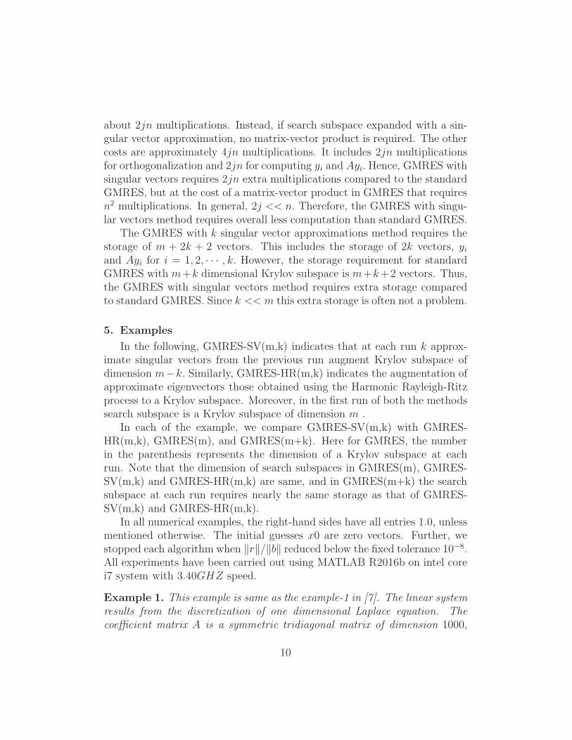
The Figure-1 depicts the convergence of residual norms and correspondingerror norms in the GMRES-SV(20,4), GMRES-HR(20,4), GMRES(20), andstandard GMRES(24) methods.

0 1000 2000 3000 4000 5000 6000 7000

Matrix vector products

-8

-7

-6

-5

-4

-3

-2

-1

0

log

10

of

resid

ua

l n

orm

Residuals Vs Matrix vector products

GMRES-SV(20,2)GMRES-HR(20,2)GMRES(22)GMRES(20)

0 1000 2000 3000 4000 5000 6000 7000


-5

-4

-3

-2

-1

0

1

2

log

10

of

err

or

no

rm

Errors Vs Matrix vector products


Figure 1: Magnitudes of ‖r‖‖b‖

with GMRES(20,4) singular vectors/eigenvectors, GMRES(24), and GM-

RES(20) (left). Absolute errors with GMRES(20,4) singular vectors/eigenvectors, GMRES(24), and GM-RES(20) (right).

In GMRES-SV(20,4), ‖r‖/‖b‖ drops to below the tolerance 10−8 in the148th run. It required 2365 number of matrix-vector products. In the re-maining three methods ‖r‖/‖b‖ did not reached at least 10−4 even after 5000matrix-vector products. Here, the total number of matrix-vector products inall methods counted in a similar way as in [3].

Observe from the right part of Figure-1 that GMRES-SV(20,4) reduceserror norms also to a far better extent than the remaining three methods.Here, error norm is the norm of an error vector, a difference between asolution obtained using ”backslash” command in Matlab and an approximatesolution in an iterative method.

From the Figure-1, we observed that when residual norm drops below thetolerance 10−8, the log 10 of an error norm in the GMRES-SV(20,4) is−4.763.In the other three methods, at 5000th matrix-vector product it is just near1.244. Therefore, this example illustrates the fact that the augmentation of

11

a Krylov subspace with singular vectors reduces error norms and also theresidual norms.

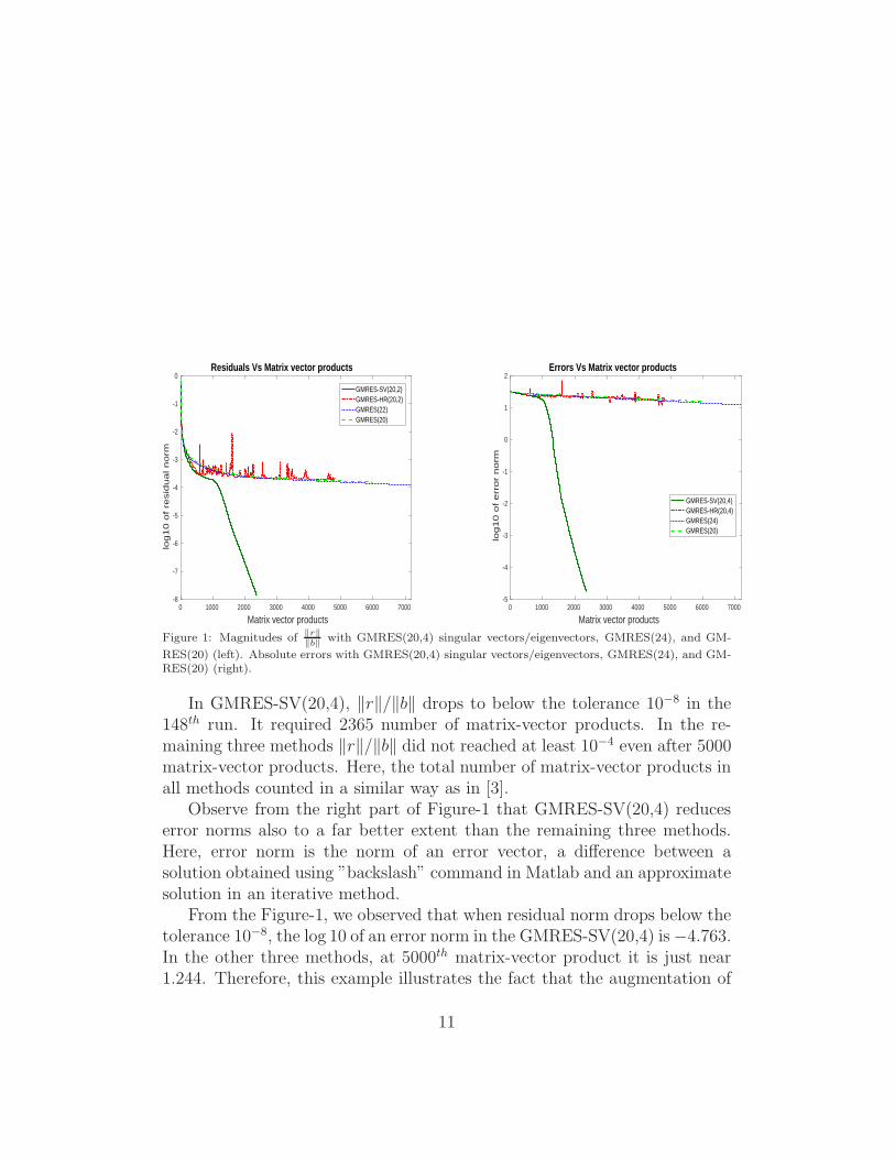
Example 2. Consider the matrix SHERMAN4 that comes from Oil reser-voir modeling. It is a real un-symmetric matrix of order 1104. The Matrixmarket provided the right-hand side vector. We compare GMRES-SV(20,4)(16 Krylov vectors and 4 approximate right singular vectors) with GMRES-HR(20,4), GMRES(20), and GMRES(24).

See left part of Figure 2 for the convergence of log10 of residual norms inall the methods.

0 100 200 300 400 500 600 700


-7

-6

-5

-4

-3

-2

-1

0

1

2

log

10

of

resid

ua

l n

orm



0 100 200 300 400 500 600 700


-8

-6

-4

-2

0

2

4

log

10

of

err

or

no

rm






In GMRES-SV(20,4) the quantity ‖r‖/‖b‖ reduced to below 10−8 at the12th run. The total number of matrix-vector products it required is 190.GMRES-HR(20,4) required 562 matrix vector products to drop ‖r‖/‖b‖below the tolerance 10−8. Thus, GMRES-HR had required nearly thricethe computation than the GMRES-SV method. Further, observe from theFigure-2 that GMRES-SV(20,4) is far better than GMRES(24) even thoughit used smaller search subspaces.

The right part of the Figure-2 compares error norms. When the residualnorm reached the tolerance, the log 10 of an error norm in GMRES-SV(20,4)is−6.063, whereas it is −5.063 in GMRES-HR(20,4), and is equal to −4.813,

12

−4.802 in the GMRES(24) and GMRES(20) methods respectively. There-fore, for this example, the GMRES-SV method significantly reduced the errornorm compared to the remaining three methods.

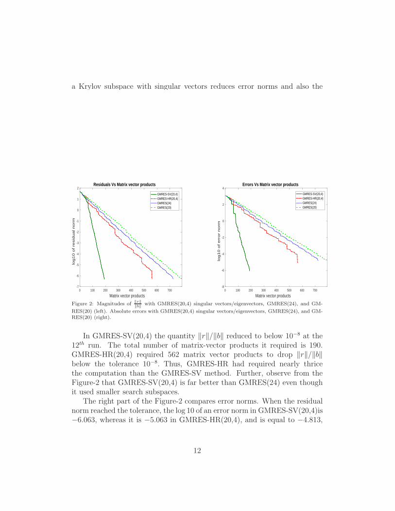
Example 3. Consider the matrix WATT1 that came from petroleum engi-neering. It is a real un-symmetric matrix of order 1856 with 11360 non-zeroentries. The right-hand side is the one provided by the Matrix Market. Tosee the performance of GMRES-SV with fewer approximate singular vectors,we have chosen m = 20 and k = 2. Thus, we have used only two approximatesingular vectors, which are less in number compared to the previous examples.

0 500 1000 1500 2000 2500


-7

-6

-5

-4

-3

-2

-1

0

1

2

log

10

of

resid

ua

l n

orm



0 500 1000 1500 2000 2500


2

3

4

5

6

7

8

9

10

11

12

log

10

of

err

or

no

rm






Using GMRES-SV(20,2), the ratio ‖r‖/‖b‖ reached the required tolerancein the 30th run, whereas in GMRES-HR(20,2), GMRES(22), and GMRES(20)it happened in 82nd, 109th, and 143rd run respectively. See Figure-3(left) forthe comparison of log 10 of residual norms in all the four methods.

Figure-3(right), compares the convergence of error norms in four methods.Observe from it that GMRES-SV(20,2) reduced the error norm to a betterextent compared to the other three methods, even though it took fewer it-erations for the convergence of ‖r‖/‖b‖. Also, it reduced residual norms aswell.

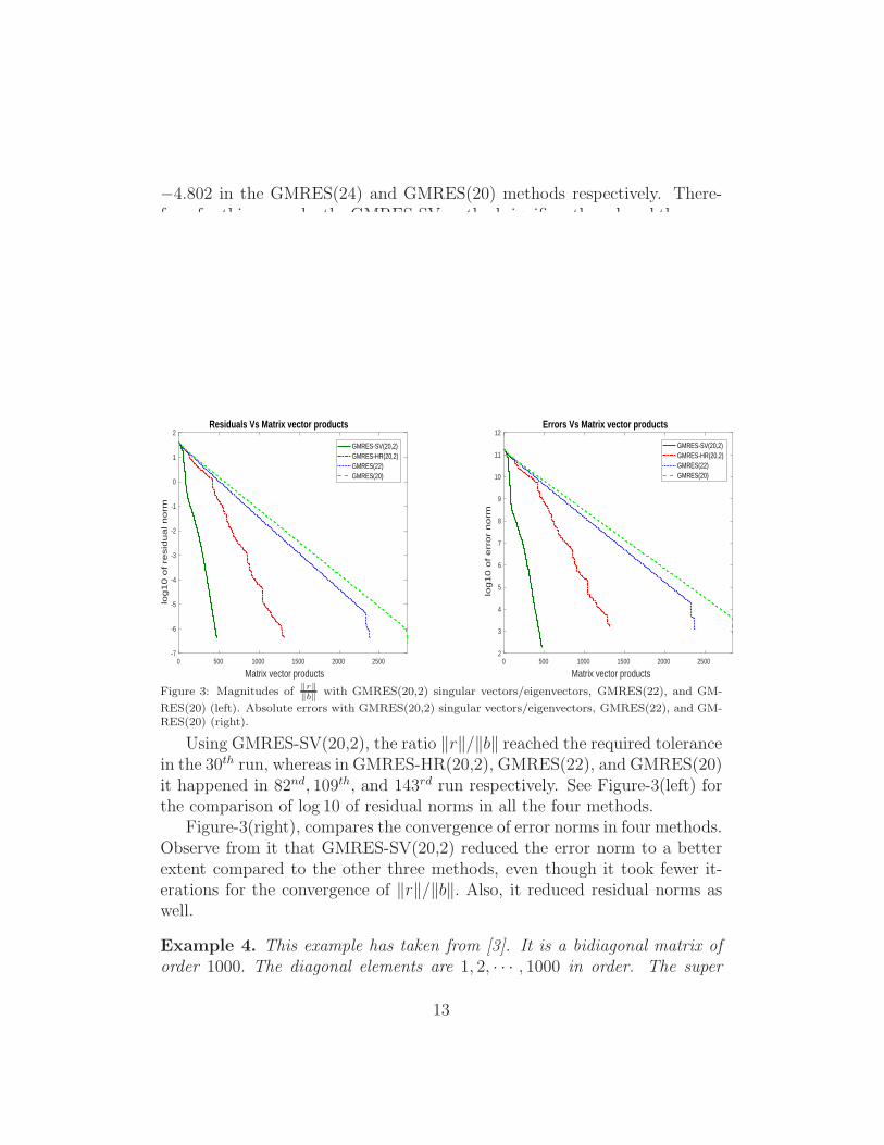
Example 4. This example has taken from [3]. It is a bidiagonal matrix oforder 1000. The diagonal elements are 1, 2, · · · , 1000 in order. The super

13

diagonal elements are 0.1s. We have chosen m = 20 and k = 2 for GMRESmethod with singular vectors. We used only two eigenvector approximationsin GMRES-HR. We compare these two methods with GMRES(20) and GM-RES(22).

0 50 100 150 200 250 300 350 400 450


-7

-6

-5

-4

-3

-2

-1

0

1

2

log

10

of

resid

ua

l n

orm



0 50 100 150 200 250 300 350 400 450


-7

-6

-5

-4

-3

-2

-1

0

1

log

10

of

err

or

no

rm



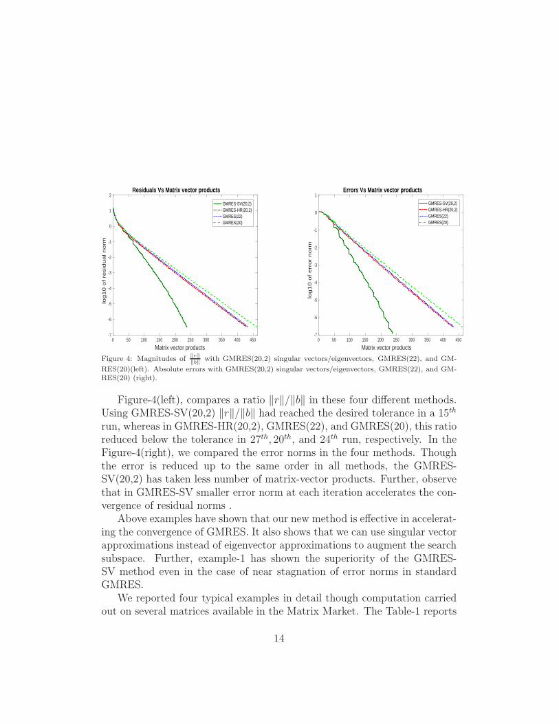
Figure 4: Magnitudes of‖r‖‖b‖


RES(20)(left). Absolute errors with GMRES(20,2) singular vectors/eigenvectors, GMRES(22), and GM-RES(20) (right).

Figure-4(left), compares a ratio ‖r‖/‖b‖ in these four different methods.Using GMRES-SV(20,2) ‖r‖/‖b‖ had reached the desired tolerance in a 15th

run, whereas in GMRES-HR(20,2), GMRES(22), and GMRES(20), this ratioreduced below the tolerance in 27th, 20th, and 24th run, respectively. In theFigure-4(right), we compared the error norms in the four methods. Thoughthe error is reduced up to the same order in all methods, the GMRES-SV(20,2) has taken less number of matrix-vector products. Further, observethat in GMRES-SV smaller error norm at each iteration accelerates the con-vergence of residual norms .

Above examples have shown that our new method is effective in accelerat-ing the convergence of GMRES. It also shows that we can use singular vectorapproximations instead of eigenvector approximations to augment the searchsubspace. Further, example-1 has shown the superiority of the GMRES-SV method even in the case of near stagnation of error norms in standardGMRES.

We reported four typical examples in detail though computation carriedout on several matrices available in the Matrix Market. The Table-1 reports

14

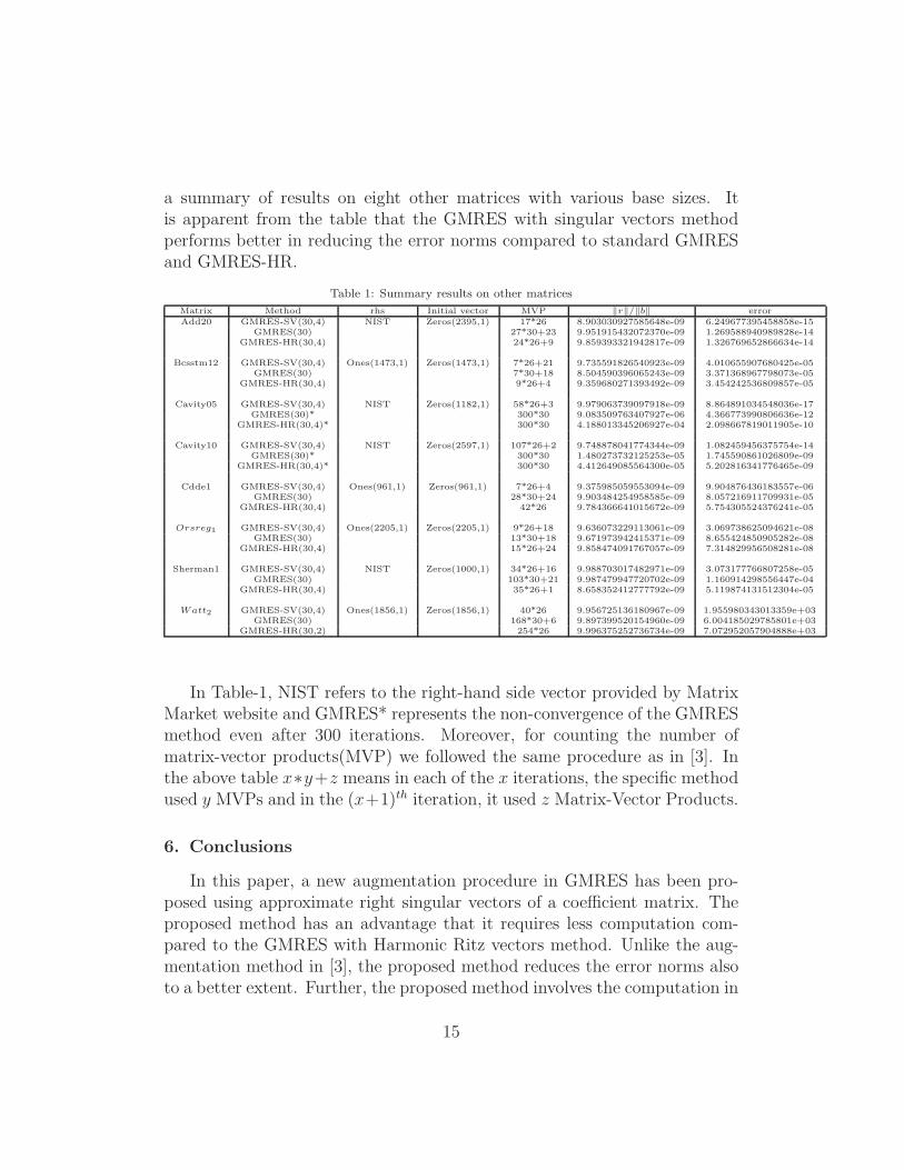
a summary of results on eight other matrices with various base sizes. Itis apparent from the table that the GMRES with singular vectors methodperforms better in reducing the error norms compared to standard GMRESand GMRES-HR.

Table 1: Summary results on other matrices

Matrix Method rhs Initial vector MVP ‖r‖/‖b‖ errorAdd20 GMRES-SV(30,4) NIST Zeros(2395,1) 17*26 8.903030927585648e-09 6.249677395458858e-15

GMRES(30) 27*30+23 9.951915432072370e-09 1.269588940989828e-14GMRES-HR(30,4) 24*26+9 9.859393321942817e-09 1.326769652866634e-14

Bcsstm12 GMRES-SV(30,4) Ones(1473,1) Zeros(1473,1) 7*26+21 9.735591826540923e-09 4.010655907680425e-05GMRES(30) 7*30+18 8.504590396065243e-09 3.371368967798073e-05

GMRES-HR(30,4) 9*26+4 9.359680271393492e-09 3.454242536809857e-05

Cavity05 GMRES-SV(30,4) NIST Zeros(1182,1) 58*26+3 9.979063739097918e-09 8.864891034548036e-17GMRES(30)* 300*30 9.083509763407927e-06 4.366773990806636e-12

GMRES-HR(30,4)* 300*30 4.188013345206927e-04 2.098667819011905e-10

Cavity10 GMRES-SV(30,4) NIST Zeros(2597,1) 107*26+2 9.748878041774344e-09 1.082459456375754e-14GMRES(30)* 300*30 1.480273732125253e-05 1.745590861026809e-09

GMRES-HR(30,4)* 300*30 4.412649085564300e-05 5.202816341776465e-09

Cdde1 GMRES-SV(30,4) Ones(961,1) Zeros(961,1) 7*26+4 9.375985059553094e-09 9.904876436183557e-06GMRES(30) 28*30+24 9.903484254958585e-09 8.057216911709931e-05

GMRES-HR(30,4) 42*26 9.784366641015672e-09 5.754305524376241e-05

Orsreg1 GMRES-SV(30,4) Ones(2205,1) Zeros(2205,1) 9*26+18 9.636073229113061e-09 3.069738625094621e-08GMRES(30) 13*30+18 9.671973942415371e-09 8.655424850905282e-08

GMRES-HR(30,4) 15*26+24 9.858474091767057e-09 7.314829956508281e-08

Sherman1 GMRES-SV(30,4) NIST Zeros(1000,1) 34*26+16 9.988703017482971e-09 3.073177766807258e-05GMRES(30) 103*30+21 9.987479947720702e-09 1.160914298556447e-04

GMRES-HR(30,4) 35*26+1 8.658352412777792e-09 5.119874131512304e-05

Watt2 GMRES-SV(30,4) Ones(1856,1) Zeros(1856,1) 40*26 9.956725136180967e-09 1.955980343013359e+03GMRES(30) 168*30+6 9.897399520154960e-09 6.004185029785801e+03

GMRES-HR(30,2) 254*26 9.996375252736734e-09 7.072952057904888e+03

In Table-1, NIST refers to the right-hand side vector provided by MatrixMarket website and GMRES* represents the non-convergence of the GMRESmethod even after 300 iterations. Moreover, for counting the number ofmatrix-vector products(MVP) we followed the same procedure as in [3]. Inthe above table x∗y+z means in each of the x iterations, the specific methodused y MVPs and in the (x+1)th iteration, it used z Matrix-Vector Products.

6. Conclusions

In this paper, a new augmentation procedure in GMRES has been pro-posed using approximate right singular vectors of a coefficient matrix. Theproposed method has an advantage that it requires less computation com-pared to the GMRES with Harmonic Ritz vectors method. Unlike the aug-mentation method in [3], the proposed method reduces the error norms alsoto a better extent. Further, the proposed method involves the computation in

15

real arithmetic for the matrices and right-hand side vectors in the real num-ber system. Numerical experiments have been carried out on benchmarkmatrices. Results have shown the superiority of the proposed method overthe standard GMRES and GMRES with Harmonic Ritz vectors methods.

Acknowledgements

The author thanks the National Board of Higher Mathematics, India forsupporting this work under the Grant number2/40(3)/2016/R&D-II/9602 .

References

References

[1] R. Ehrig and Peter D.Euflhard, GMERR as an Error Minimizing Vari-ant of GMRES, Preprint SC 97-63, Konrad-Zuse-Zentrum fur Informa-tionstechnik Berlin, 1997.

[2] Chunguang Li, CGNR Is an Error Reducing Algorithm, SIAM Journalon Scientific Computing, 22:6 (2001), 2109-2112.

[3] R.B. Morgan, A restarted GMRES method augmented with eigenvectors,SIAM J. Matrix Anal. Appl., 16:4 (1995), pp. 1154 - 1171.

[4] M. Rozloznık, R. Weiss, On the stable implementation of the generamizedminimal error method, Journal of Computational and Applied Mathe-matics, 98 (1998), pp. 49 - 62.

[5] Y. Saad, M.H. Schultz, GMRES: a generalized minimal residual algo-rithm for solving nonsymmetric linear systems, SIAM J. Sci. Stat. Com-put., 7 (1986), pp. 856 - 869.

[6] Y. Saad, Analysis of augmented Krylov subspace methods, SIAM J. Ma-trix. Anal. Appl., 18:2 (1997), pp. 435 -449.

[7] R. Weiss, Error minimizing Krylov subspace methods, SIAMJ.Sci.Comp., 15 (1994), pp.511-527.

[8] J. Zitko, Some remarks on the restarted and augmented GMRES method,Electron. Trans. Numer. Anal., 31 (2008), pp. 221 - 227.

16

Documents

GMRES with Singular Vector Approximations - arXiv