Embed Size (px)
Citation preview
Geosci. Model Dev., 8, 317–340, 2015
www.geosci-model-dev.net/8/317/2015/
doi:10.5194/gmd-8-317-2015
© Author(s) 2015. CC Attribution 3.0 License.
ASAM v2.7: a compressible atmospheric model with
a Cartesian cut cell approach
M. Jähn, O. Knoth, M. König, and U. Vogelsberg
Leibniz Institute for Tropospheric Research, Permoserstrasse 15, 04318 Leipzig, Germany
Correspondence to: M. Jähn ([email protected])
Received: 16 June 2014 – Published in Geosci. Model Dev. Discuss.: 18 July 2014
Revised: 19 January 2015 – Accepted: 22 January 2015 – Published: 18 February 2015
Abstract. In this work, the fully compressible, three-
dimensional, nonhydrostatic atmospheric model called All
Scale Atmospheric Model (ASAM) is presented. A cut cell
approach is used to include obstacles and orography into
the Cartesian grid. Discretization is realized by a mixture
of finite differences and finite volumes and a state limit-
ing is applied. Necessary shifting and interpolation tech-
niques are outlined. The method can be generalized to any
other orthogonal grids, e.g., a lat–long grid. A linear im-
plicit Rosenbrock time integration scheme ensures numeri-
cal stability in the presence of fast sound waves and around
small cells. Analyses of five two-dimensional benchmark
test cases from the literature are carried out to show that
the described method produces meaningful results with re-
spect to conservation properties and model accuracy. The
test cases are partly modified in a way that the flow field or
scalars interact with cut cells. To make the model applicable
for atmospheric problems, physical parameterizations like a
Smagorinsky subgrid-scale model, a two-moment bulk mi-
crophysics scheme, and precipitation and surface fluxes us-
ing a sophisticated multi-layer soil model are implemented
and described. Results of an idealized three-dimensional
simulation are shown, where the flow field around an ide-
alized mountain with subsequent gravity wave generation,
latent heat release, orographic clouds and precipitation are
modeled.
1 Introduction
In this paper we present the numerical solver ASAM (All
Scale Atmospheric Model) that has been developed at the
Leibniz Institute for Tropospheric Research (TROPOS),
Leipzig. ASAM was initially designed for CFD (compu-
tational fluid dynamics) simulations around buildings. The
model can also be used with spherical or cylindrical grids.
Stability problems with grid convergence in special points
(the pole problem) in both grids are handled through the im-
plicit time integration both for advection and the yet faster
gravity and acoustic waves. For simulating the flow around
obstacles, buildings or orography, the cut (or shaved) cell
approach is used. With this attempt one remains within the
Cartesian grid and the numerical pressure derivative in the
vicinity of a structure is zero if the cut cell geometry is not
taken into account, which is not the case in terrain-following
coordinate systems due to the slope of the lowest cells (Lock
et al., 2012). Since this skewness is also reproduced in upper
levels, a cut cell model produces reduced or greatly reduced
errors in comparison models with terrain-following coor-
dinates (Good et al., 2014). Several techniques have been
developed to overcome these nonphysical errors associated
with terrain-following grids, especially when spatial scales
of three-dimensional models become finer (which leads to
a steepening of the model orography). Tripoli and Smith
(2014a) introduced a variable-step topography (VST) sur-
face coordinate system within a nonhydrostatic host model.
Unlike the traditional discrete-step approach, the depth of
a grid box intersecting with a topographical structure is ad-
justed to its height, which leads to straight cut cells. Nu-
merical tests show that this technique produces better re-
sults than conventional approaches for different topography
(severe and smooth) types (Tripoli and Smith, 2014b). In
their cases, also the computational costs with the VST ap-
proach are reduced because there is no need of extra func-
tional transform calculations due to metric terms. Steppeler
et al. (2002) derived approximations for z coordinate non-
Published by Copernicus Publications on behalf of the European Geosciences Union.
318 M. Jähn et al.: ASAM v2.7
hydrostatic atmospheric models by using the shaved-element
finite volume method. There, the dynamics are computed in
the cut cell system, whereas the physics computation remains
in the terrain-following system. Using a z-coordinate system
can also improve the prediction of meteorological parame-
ters like clouds and rainfall due to a better representation of
the atmospheric flow near mountains in a numerical weather
prediction (NWP) model (Steppeler et al., 2006, 2013). The
cut cell method is also used in the Ocean–Land–Atmosphere
Model (OLAM) (Walko and Avissar, 2008a), which extends
the Regional Atmospheric Modeling System (RAMS) to
a global model domain. In OLAM, the shaved-cell method is
applied to an icosahedral mesh (Walko and Avissar, 2008b).
Yamazaki and Satomura (2008) simulated a two-dimensional
flow over different mountain slopes and compared the results
of their cut cell model with a model using terrain-following
coordinates. Especially for steep slopes, significant errors
were reported in the terrain-following model. A drawback is
the generation of low-volume cells when a cut cell method is
used. To avoid instability problems around these small cells,
the time integration scheme has to be adapted. This can be
achieved by using semi-implicit or semi-Langrangian meth-
ods, for example. In ASAM, a linear-implicit Rosenbrock
time integration scheme is used (Hairer and Wanner, 1996).
Another option to handle the small cells problem is to merge
small cut cells with neighboring cells in either the horizontal
or vertical direction (Yamazaki and Satomura, 2010). How-
ever, this approach becomes more complicated when apply-
ing it to three spatial dimensions, since a lot of special cases
have to be considered. To achieve reasonable vertical solu-
tions near the ground, the usage of local mesh refinement
techniques becomes interesting for large-scale models (Ya-
mazaki and Satomura, 2012).
The here-presented model is a developing research code
with different options to choose from like different numeri-
cal methods (e.g., split-explicit Runge–Kutta or partially im-
plicit peer schemes), number of prognostic variables, physi-
cal parameterizations or the change to a spherical grid type.
Parallelization is realized by using the message passing inter-
face (MPI) and the domain decomposition method. The code
is easily portable between different platforms like Linux,
IBM or Mac OS. With these features, large eddy simulations
(LES) with spatial resolutions of O(1–100 m) can be per-
formed with respect to a sufficiently resolved terrain struc-
ture. In previous studies, the model was used to demonstrate
the volume-of-fluid (VOF) method for nondissipative cloud
transport (Hinneburg and Knoth, 2005). ASAM also took
part in an intercomparison study of mountain-wave simula-
tions for idealized and real terrain profiles, where altogether
11 different nonhydrostatic numerical models were com-
pared (Doyle et al., 2011). A partially implicit peer method
is presented in Jebens et al. (2011) in order to overcome the
small cell problem around orography when using cut cells.
The model was recently used for a study of dynamic flow
structures in a turbulent urban environment of a building-
resolving resolution (König, 2013). There, the implementa-
tion of a dynamic Smagorinsky subgrid-scale model is tested
for a convective atmospheric boundary layer and an inflow
generation approach that produces a turbulent flow field is
presented.
A separately developed LES model at TROPOS is called
ASAMgpu (Horn, 2012). It includes some basic features
of the ASAM code and runs on graphics processing units
(GPUs), which enables very time-efficient computations and
post-processing. However, this model is not as adjustable
as the original ASAM code and the inclusion of three-
dimensional orographical structures is not implemented so
far. ASAMgpu was applied for a study of heat island effects
on vertical mixing of aerosols by comparing the results of
large eddy simulations with wind and aerosol lidar observa-
tions (Engelmann et al., 2011).
This paper is structured as follows. The next section deals
with a general description of the model. It includes the ba-
sic equations that are solved numerically and the used energy
variable. Also, the cut cell approach and spatial discretization
as well as the time integration scheme are described. This ap-
proach can be extended to other orthogonal grids like the lat–
long grid. Section 3 deals with the model physics, including
a subgrid-scale model, a two-moment microphysics scheme
and surface flux parameterization. Results of different ideal-
ized test cases are shown in Sect. 4. The first one is a dry ris-
ing heat bubble described by Wicker and Skamarock (1998)
followed by a flow past an idealized mountain ridge from
Schaer et al. (2002). Two other “classical” test examples have
been chosen and modified so that cut cells are included and
interaction within these cells are guaranteed. The first one is a
falling cold bubble with a developing density current (Straka
et al., 1993) but with a 1 km high mountain on the left part of
the domain. The second case is the moist bubble benchmark
case reported by Bryan and Fritsch (2002). The bubble will
rise and interact with a zeppelin-shaped cut area in the center
of the domain. For both test cases, energy conservation tests
are carried out. Another two-dimensional case by Berger and
Helzel (2012) is presented to test the accuracy of the cut
cell method by advecting a smooth bump in a radial wind
field in an annulus. For the last test case, a three-dimensional
mountain overflow with subsequent orographic cloud gener-
ation and precipitation is simulated (Kunz and Wassermann,
2011). Concluding remarks and future work are in the final
section.
2 Description of the All Scale Atmospheric Model
2.1 Governing equations
The flux-form compressible Euler equations for the atmo-
sphere are
Geosci. Model Dev., 8, 317–340, 2015 www.geosci-model-dev.net/8/317/2015/
M. Jähn et al.: ASAM v2.7 319
Table 1. Physical constants.
Symbol Quantity Value
p0 Reference pressure 105 Pa
Rd Gas constant for dry air 287 Jkg−1 K−1
Rv Gas constant for water vapor 461 Jkg−1 K−1
cpd Specific heat capacity at constant pressure for dry air 1004 Jkg−1 K−1
cpv Specific heat capacity at constant pressure for water vapor 1885 Jkg−1 K−1
cpl Specific heat capacity at constant pressure for liquid water 4186 Jkg−1 K−1
cvd Specific heat capacity at constant volume for dry air 717 Jkg−1 K−1
cvv Specific heat capacity at constant volume for water vapor 1424 Jkg−1 K−1
L00 Latent heat at 0 K 3.148× 10⁶ Jkg−1
g Gravitational acceleration 9.81 ms−2
Cs Smagorinsky coefficient 0.2
∂ρ
∂t+∇ · (ρv)= 0, (1)
∂(ρv)
∂t+∇ · (ρvv)=−∇ · τ −∇p− ρg− 2�× (ρv), (2)
∂(ρφ)
∂t+∇ · (ρvφ)=−∇ · qφ + Sφ, (3)
where ρ is the total air density, v = (u,v,w)T the three-
dimensional velocity vector, p the air pressure, g the grav-
itational acceleration, � the angular velocity vector of the
earth, φ a scalar quantity and Sφ the sum of its corresponding
source terms. The subgrid-scale terms are τ for momentum
and qφ for a given scalar.
The energy equation in the form of Eq. (3) is represented
by the (dry) potential temperature θ . In the presence of wa-
ter vapor and cloud water, this quantity is replaced by the
density potential temperature θρ (Emanuel, 1994) as a more
generalized form of the virtual potential temperature θv:
θρ = θ
(1+ qv
[Rv
Rd
− 1
]− qc
), (4)
where the equation of state can be expressed as follows:
p = ρRdθρ
(p
p0
)κm
. (5)
In the previous two equations θ = T (p0/p)κm is the potential
temperature, qv = ρv/ρ is the mass ratio of water vapor in the
air (specific humidity), qc = ρc/ρ is the mass ratio of cloud
water in the air, p0 a reference pressure and κm = (qdRd+
qvRv)/(qdcpd+qvcpv+qccpl) the Poisson constant for the air
mixture (dry air, water vapor, cloud water) with qd = ρd/ρ.
Rd and Rv are the gas constants for dry air and water vapor,
respectively.
The number of additional equations like Eq. (3) depends
on the complexity of the microphysical scheme used. Fur-
thermore, tracer variables can also be included. The values
of all relevant physical constants are listed in Table 1.
2.2 Cut cells and spatial discretization
2.2.1 Definition of cut cells
The spatial discretization is done on a Cartesian grid with
grid intervals of lengths 1xi,1yj ,1zk and can easily be
extended to any orthogonal, logically rectangular structured
grid (i.e., it has the same logical structure as a regular Carte-
sian grid) like spherical or cylindrical coordinates. First, it
is described for the Cartesian case. Generalizations are dis-
cussed afterwards. Orography and other obstacles like build-
ings are presented by cut cells, which are the result of the
intersection of the obstacle with the underlying Cartesian
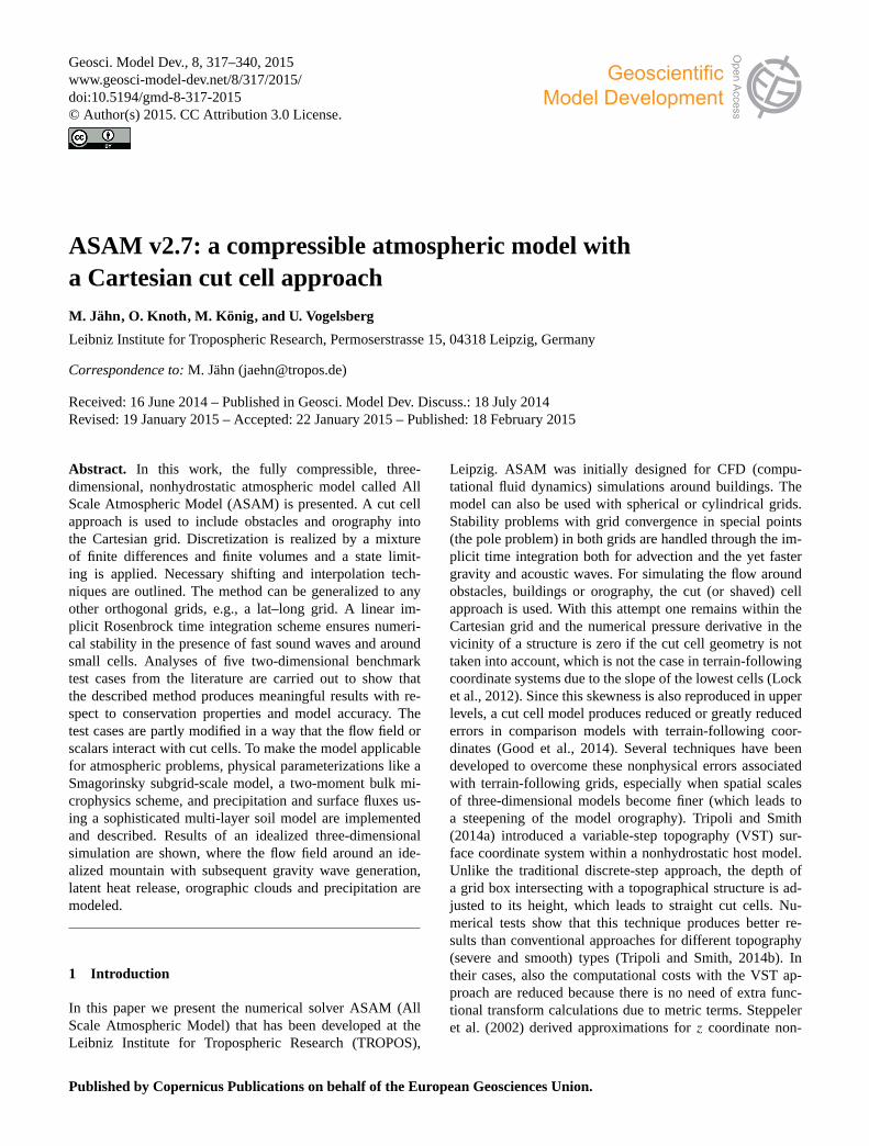
grid. In Fig. 1 different possible and excluded configurations
are shown for the three-dimensional case. For the spatial
discretization only the six partial face areas and the partial
cell volume and the grid sizes of the underlying Cartesian
mesh are used. For a proper representation the orography is
smoothed in such a way that the intersection of a grid cell
and the orography can be described by a single possible non-
planar polygon. Or in other words, a Cartesian cell is divided
in at most two parts, a free part and a solid part. For each
Cartesian cell, the free face area of the six faces and the free
volume area of the cell are stored, which is the part outside
of the obstacle. These values are denoted for the grid cell
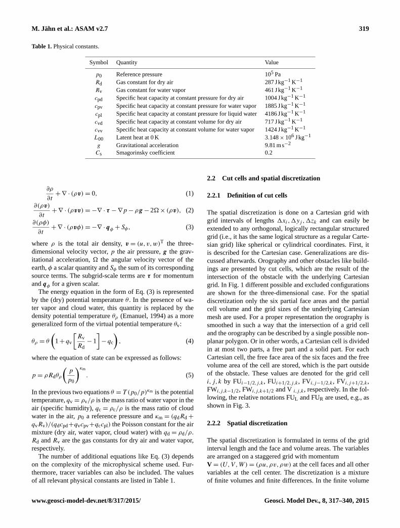
i,j,k by FUi−1/2,j,k , FUi+1/2,j,k , FVi,j−1/2,k , FVi,j+1/2,k ,
FWi,j,k−1/2, FWi,j,k+1/2 and V i,j,k , respectively. In the fol-
lowing, the relative notations FUL and FUR are used, e.g., as
shown in Fig. 3.
2.2.2 Spatial discretization
The spatial discretization is formulated in terms of the grid
interval length and the face and volume areas. The variables
are arranged on a staggered grid with momentum
V= (U,V,W)= (ρu,ρv,ρw) at the cell faces and all other
variables at the cell center. The discretization is a mixture
of finite volumes and finite differences. In the finite volume
www.geosci-model-dev.net/8/317/2015/ Geosci. Model Dev., 8, 317–340, 2015
320 M. Jähn et al.: ASAM v2.7
Discussion
Paper
|D
iscussionPaper
|D
iscussionPaper
|D
iscussionPaper
|
4 M. Jahn: ASAM v2.7
��������������������������������������������������������
��������������������������������������������������������
������������
������������
���������
���������
��������������������������������������������������
��������������������������������������������������
������������������������������������������
������������������������������������������
������������
������������
4 markers3 markers 5 markers 6 markers 6 markers
Fig. 1. Possible configurations for cut cell intersection. The last two cases are excluded.
............................
............................
............................
............................
............................
............................
............................
............................
...............
FUL FUR
FWL
FWR
FC
VC
.
.
.
.
.
.
.
.
.
.
.
.
.
.
.
.
.
.
.
.
.
.
.
.
.
.
.
.
.
.
.
.
.
.
.
.
.
.
.
.
.
.
.
.
.
.
.
.
.
.
.
.
.
.
.
.
.
.
.
.
.
.
.
.
.
.
.
.
.
.
.
.
.
.
.
.
.
.
.
.
.
.
.
.
.
.
.
.
.
.
.
.
.
.
.
.
.
.
.
.
.
.
.
.
.
.
.
.
.
.
.
.
.
.
.
.
.
.
.
.
.
.
.
.
.
.
.
.
.
.
.
.
.
.
.
.
.
.
.
.
.
.
.
.
.
.
.
.
.
.
.
.
.
.
.
.
.
.
.
.
.
.
.
.
.
.
.
.
.
.
..............................................................................................................................................................................................................................................................................................
........................................................................................................................................................................................................................................................................................................................................................................................................ ......................................................................................................................................................................................................................................................................................................................................................................................................................................................................................................................................................................................................................................................................................................
UFURC ULC...................................................................... .................................................
Fig. 2. Cut cell with face and volume area information (left) and arrangement of face and cell centered momentum (right).
hL hC hR
φL φC φR
-UR > 0
Fig. 3. Stencil for third-order approximation.
2.3 Time integration
After spatial discretization an ordinary differential equation
y(t)′ = F (y(t)) (15)
is obtained that has to be integrated in time (method of lines).To tackle the small time step problem connected with tiny230
cut cells, linear implicit Rosenbrock-W-methods are used(Jebens et al., 2011).
A Rosenbrock method has the form
(I − τγJ)ki =τF (yn +i−1∑
j=1
αijuj) +i−1∑
j=1
βijkj , i= 1, ...,s
(16)
yn+1 =yn +s∑
j=1
αs+1jkj ,235
where yn is a given approximation at y(t) at time tn andsubsequently yn+1 at time tn+1 = tn+ τ . In addition J is anapproximation to the Jacobian matrix ∂F/∂y. A Rosenbrockmethod is therefore fully described by the two matrices A=240
(αij), Γ = (γij) and the parameter γ.Among the available methods are a second order two stage
method after Lanser et al. (2001).
Sk1 =τF (yn) , (17)
Sk2 =τF
(yn +
2
3k1
)− 4
3k1 , (18)245
yn+1 =yn +5
4k1 +
3
4k2 , (19)
S =I − γτJ, J ≈ F ′(yn) . (20)
with γ =1
2+
1
6
√3 or in matrix form in Table (2).
02/3
−5/4 3/4−4/3
12
+ 16
√3
A-Matrix Γ-Matrix γ
Table 2. Coefficient table for ROS2.
A second method was constructed from a low stor-250
age three stage second-order Runge-Kutta method, whichis used in split-explicit time integration methods in theWeather Research and Forecasting (WRF) Model (Ska-marock et al., 2008) or in the Consortium for Small-scale
Figure 1. Possible configurations for cut cell intersection (cases 1–3) for different numbers of faceintersection points (markers). The last two cases are excluded.
53
Figure 1. Possible configurations for cut cell intersection (cases 1–3) for different numbers of face intersection points (markers). The last
two cases are excluded.
Discussion
Paper
|D
iscussionPaper
|D
iscussionPaper
|D
iscussionPaper
|
4 M. Jahn: ASAM v2.7
��������������������������������������������������������
��������������������������������������������������������
������������
������������
���������
���������
��������������������������������������������������
��������������������������������������������������
������������������������������������������
������������������������������������������
������������
������������
4 markers3 markers 5 markers 6 markers 6 markers
Fig. 1. Possible configurations for cut cell intersection. The last two cases are excluded.
............................
............................
............................
............................
............................
............................
............................
............................
...............
FUL FUR
FWL
FWR
FC
VC
.
.
.
.
.
.
.
.
.
.
.
.
.
.
.
.
.
.
.
.
.
.
.
.
.
.
.
.
.
.
.
.
.
.
.
.
.
.
.
.
.
.
.
.
.
.
.
.
.
.
.
.
.
.
.
.
.
.
.
.
.
.
.
.
.
.
.
.
.
.
.
.
.
.
.
.
.
.
.
.
.
.
.
.
.
.
.
.
.
.
.
.
.
.
.
.
.
.
.
.
.
.
.
.
.
.
.
.
.
.
.
.
.
.
.
.
.
.
.
.
.
.
.
.
.
.
.
.
.
.
.
.
.
.
.
.
.
.
.
.
.
.
.
.
.
.
.
.
.
.
.
.
.
.
.
.
.
.
.
.
.
.
.
.
.
.
.
.
.
.
..............................................................................................................................................................................................................................................................................................
........................................................................................................................................................................................................................................................................................................................................................................................................ ......................................................................................................................................................................................................................................................................................................................................................................................................................................................................................................................................................................................................................................................................................................
UFURC ULC...................................................................... .................................................
Fig. 2. Cut cell with face and volume area information (left) and arrangement of face and cell centered momentum (right).
hL hC hR
φL φC φR
-UR > 0
Fig. 3. Stencil for third-order approximation.
2.3 Time integration
After spatial discretization an ordinary differential equation
y(t)′ = F (y(t)) (15)
is obtained that has to be integrated in time (method of lines).To tackle the small time step problem connected with tiny230
cut cells, linear implicit Rosenbrock-W-methods are used(Jebens et al., 2011).
A Rosenbrock method has the form
(I − τγJ)ki =τF (yn +i−1∑
j=1
αijuj) +i−1∑
j=1
βijkj , i= 1, ...,s
(16)
yn+1 =yn +s∑
j=1
αs+1jkj ,235
where yn is a given approximation at y(t) at time tn andsubsequently yn+1 at time tn+1 = tn+ τ . In addition J is anapproximation to the Jacobian matrix ∂F/∂y. A Rosenbrockmethod is therefore fully described by the two matrices A=240
(αij), Γ = (γij) and the parameter γ.Among the available methods are a second order two stage
method after Lanser et al. (2001).
Sk1 =τF (yn) , (17)
Sk2 =τF
(yn +
2
3k1
)− 4
3k1 , (18)245
yn+1 =yn +5
4k1 +
3
4k2 , (19)
S =I − γτJ, J ≈ F ′(yn) . (20)
with γ =1
2+
1
6
√3 or in matrix form in Table (2).
02/3
−5/4 3/4−4/3
12
+ 16
√3
A-Matrix Γ-Matrix γ
Table 2. Coefficient table for ROS2.
A second method was constructed from a low stor-250
age three stage second-order Runge-Kutta method, whichis used in split-explicit time integration methods in theWeather Research and Forecasting (WRF) Model (Ska-marock et al., 2008) or in the Consortium for Small-scale
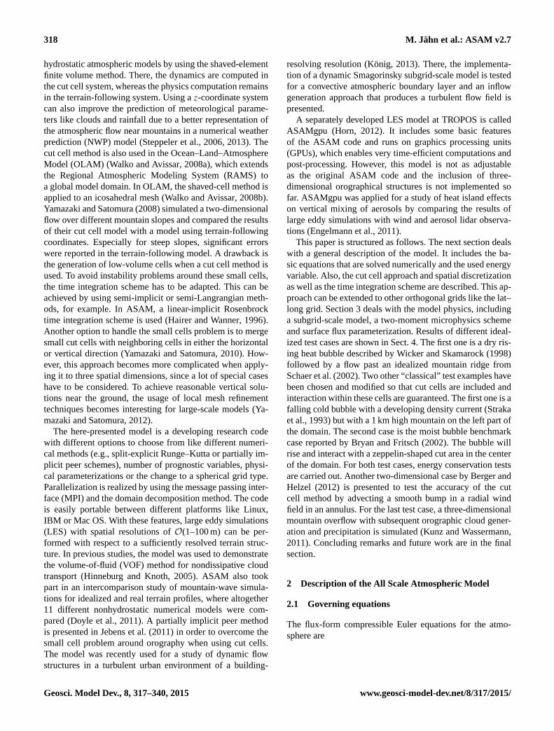
Figure 2. Stencil for third-order approximation.
54
Figure 2. Stencil for third-order approximation.
Discussion
Paper
|D
iscussionPaper
|D
iscussionPaper
|D
iscussionPaper
|
............................
............................
............................
............................
............................
............................
............................
............................
...............
FUL FUR
FWL
FWR
FC
VC
.
.
.
.
.
.
.
.
.
.
.
.
.
.
.
.
.
.
.
.
.
.
.
.
.
.
.
.
.
.
.
.
.
.
.
.
.
.
.
.
.
.
.
.
.
.
.
.
.
.
.
.
.
.
.
.
.
.
.
.
.
.
.
.
.
.
.
.
.
.
.
.
.
.
.
.
.
.
.
.
.
.
.
.
.
.
.
.
.
.
.
.
.
.
.
.
.
.
.
.
.
.
.
.
.
.
.
.
.
.
.
.
.
.
.
.
.
.
.
.
.
.
.
.
.
.
.
.
.
.
.
.
.
.
.
.
.
.
.
.
.
.
.
.
.
.
.
.
.
.
.
.
.
.
.
.
.
.
.
.
.
.
.
.
.
.
.
.
.
.
..............................................................................................................................................................................................................................................................................................
........................................................................................................................................................................................................................................................................................................................................................................................................ ......................................................................................................................................................................................................................................................................................................................................................................................................................................................................................................................................................................................................................................................................................................
UFURC ULC................................................. .................................................
Figure 3. Cut cell with face and volume area information (left) and arrangement of face and cellcentered momentum (right).
55
Figure 3. Cut cell with face and volume area information (left) and
arrangement of face- and cell-centered momentum (right).
context the main task is the reconstruction of values and gra-
dients at cell faces from cell-centered values.
The discretization of the advection operator is performed
for a generic cell-centered scalar variable φ. In the context
of a finite volume discretization, point values of the scalar
value φ are needed at the faces of this grid cell. Knowing
these face values, the advection operator in the x direction
is discretized by (FURUFRφR−FULUFLφL)/VC where UF
is the discretized momentum at the corresponding faces. To
approximate these values at the faces, a biased upwind third-
order procedure with additional limiting is used (Van Leer,
1994).
Assuming a positive flow in the x direction, the third-order
approximation at xi+1/2 is obtained by quadratic interpola-
tion from the three values as shown in Fig. 2. The interpola-
tion condition is that the three cell-averaged values are fitted:
φFR =φC+hC(hL+hC)
(hC+hR)(hL+hC+hR)(φR−φC)
+hChR
(hL+hC)(hL+hC+hR)(φC−φL)
=φC+α1(φR−φC)+α2(φC−φL). (6)
To achieve positivity in Eq. (6), we apply state limiting. For
this task, Eq. (6) is rewritten in slope-ratio formulation:
φFR = φC+K(φC−φL) , (7)
where
K = α1
φR−φC
φC−φL
+α2. (8)
Then K is replaced by limiter function 9 and Eq. (7) is
rewritten as
φFR = φC+9
(φR−φC
φC−φL
)(φC−φL), (9)
9(r)=max(0,min[r,min(δ,α1r +α2)]) , δ = 2, (10)
as proposed by Sweby (1984). This limiter has the property
that the unlimited higher-order scheme (Eq. 6) is used as
much as possible and is utilized only then when it is needed.
In the case of 9 = 0, the scheme degenerates to the simple
first-order upwind scheme. The coefficients α1 and α2 can be
computed in advance to minimize the overhead for a nonuni-
form grid. In the case of a uniform grid the coefficients are
constant, i.e., they are equal to 1/3 and 1/6. For a detailed
discussion of the benefits of this approach and numerical ex-
periments also see Hundsdorfer et al. (1995). This procedure
is applied in all three grid directions, where the virtual grid
sizes h are defined as
hL = VL/FL, (11)
hC = 0.5VC/(FL+FR), (12)
hR = VR/FR. (13)
2.2.3 Momentum
To solve the momentum equation, the nonlinear advection
term is needed on the face. This is achieved by a shifting
technique introduced by Hicken et al. (2005) for the incom-
pressible Navier–Stokes equation. For each cell, two cell-
centered values of each of the three components of the Carte-
sian velocity vector are computed and transported with the
above advection scheme for a cell-centered scalar value. The
Geosci. Model Dev., 8, 317–340, 2015 www.geosci-model-dev.net/8/317/2015/
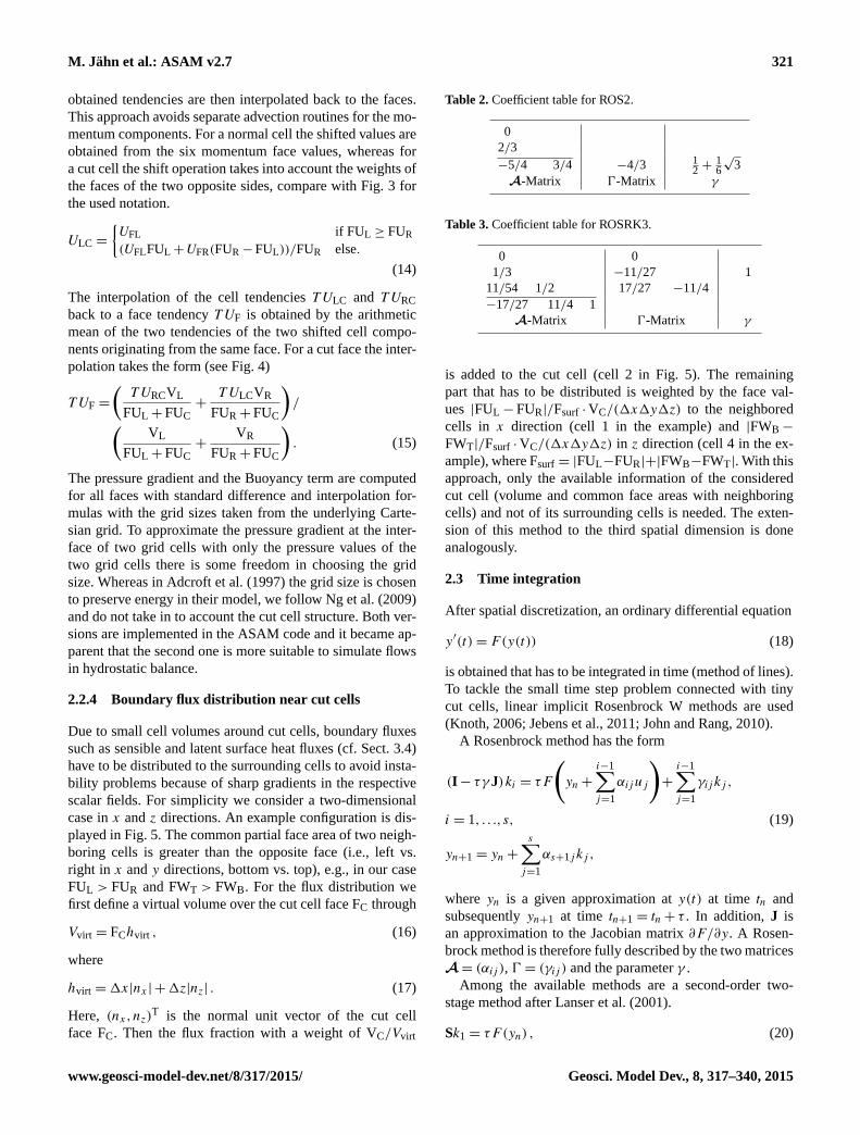
M. Jähn et al.: ASAM v2.7 321
obtained tendencies are then interpolated back to the faces.
This approach avoids separate advection routines for the mo-
mentum components. For a normal cell the shifted values are
obtained from the six momentum face values, whereas for
a cut cell the shift operation takes into account the weights of
the faces of the two opposite sides, compare with Fig. 3 for
the used notation.
ULC =
{UFL if FUL ≥ FUR
(UFLFUL+UFR(FUR−FUL))/FUR else.
(14)
The interpolation of the cell tendencies T ULC and T URC
back to a face tendency T UF is obtained by the arithmetic
mean of the two tendencies of the two shifted cell compo-
nents originating from the same face. For a cut face the inter-
polation takes the form (see Fig. 4)
T UF =
(T URCVL
FUL+FUC
+T ULCVR
FUR+FUC
)/(
VL
FUL+FUC
+VR
FUR+FUC
). (15)
The pressure gradient and the Buoyancy term are computed
for all faces with standard difference and interpolation for-
mulas with the grid sizes taken from the underlying Carte-
sian grid. To approximate the pressure gradient at the inter-
face of two grid cells with only the pressure values of the
two grid cells there is some freedom in choosing the grid
size. Whereas in Adcroft et al. (1997) the grid size is chosen
to preserve energy in their model, we follow Ng et al. (2009)
and do not take in to account the cut cell structure. Both ver-
sions are implemented in the ASAM code and it became ap-
parent that the second one is more suitable to simulate flows
in hydrostatic balance.
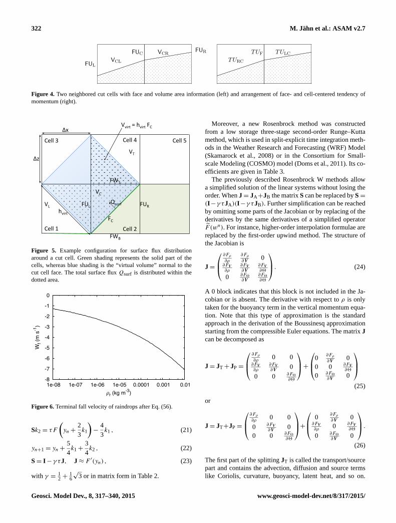
2.2.4 Boundary flux distribution near cut cells
Due to small cell volumes around cut cells, boundary fluxes
such as sensible and latent surface heat fluxes (cf. Sect. 3.4)
have to be distributed to the surrounding cells to avoid insta-
bility problems because of sharp gradients in the respective
scalar fields. For simplicity we consider a two-dimensional
case in x and z directions. An example configuration is dis-
played in Fig. 5. The common partial face area of two neigh-
boring cells is greater than the opposite face (i.e., left vs.
right in x and y directions, bottom vs. top), e.g., in our case
FUL > FUR and FWT > FWB. For the flux distribution we
first define a virtual volume over the cut cell face FC through
Vvirt = FChvirt , (16)
where
hvirt =1x|nx | +1z|nz| . (17)
Here, (nx,nz)T is the normal unit vector of the cut cell
face FC. Then the flux fraction with a weight of VC/Vvirt
Table 2. Coefficient table for ROS2.
0
2/3
−5/4 3/4 −4/3 12+
16
√3
A-Matrix 0-Matrix γ
Table 3. Coefficient table for ROSRK3.
0 0
1/3 −11/27 1
11/54 1/2 17/27 −11/4
−17/27 11/4 1
A-Matrix 0-Matrix γ
is added to the cut cell (cell 2 in Fig. 5). The remaining
part that has to be distributed is weighted by the face val-
ues |FUL−FUR|/Fsurf ·VC/(1x1y1z) to the neighbored
cells in x direction (cell 1 in the example) and |FWB−
FWT|/Fsurf ·VC/(1x1y1z) in z direction (cell 4 in the ex-
ample), where Fsurf = |FUL−FUR|+|FWB−FWT|. With this
approach, only the available information of the considered
cut cell (volume and common face areas with neighboring
cells) and not of its surrounding cells is needed. The exten-
sion of this method to the third spatial dimension is done
analogously.
2.3 Time integration
After spatial discretization, an ordinary differential equation
y′(t)= F(y(t)) (18)
is obtained that has to be integrated in time (method of lines).
To tackle the small time step problem connected with tiny
cut cells, linear implicit Rosenbrock W methods are used
(Knoth, 2006; Jebens et al., 2011; John and Rang, 2010).
A Rosenbrock method has the form
(I− τγ J)ki = τF
(yn+
i−1∑j=1
αijuj
)+
i−1∑j=1
γijkj ,
i = 1, . . ., s, (19)
yn+1 = yn+
s∑j=1
αs+1jkj ,
where yn is a given approximation at y(t) at time tn and
subsequently yn+1 at time tn+1 = tn+ τ . In addition, J is
an approximation to the Jacobian matrix ∂F/∂y. A Rosen-
brock method is therefore fully described by the two matrices
A= (αij ), 0 = (γij ) and the parameter γ .
Among the available methods are a second-order two-
stage method after Lanser et al. (2001).
Sk1 = τF (yn) , (20)
www.geosci-model-dev.net/8/317/2015/ Geosci. Model Dev., 8, 317–340, 2015
322 M. Jähn et al.: ASAM v2.7
Discussion
Paper
|D
iscussionPaper
|D
iscussionPaper
|D
iscussionPaper
|
........................................
........................................
........................................
........................................
........................................
........................................................
............................................................................
............................................................................
..................................
FUL
FURFUC
VCL
VCR
.
.
.
.
.
.
.
.
.
.
.
.
.
.
.
.
.
.
.
.
.
.
.
.
.
.
.
.
.
.
.
.
.
.
.
.
.
.
.
.
.
.
.
.
.
.
.
.
.
.
.
.
.
.
.
.
.
.
.
.
.
.
.
.
.
.
.
.
.
.
.
.
.
.
.
.
.
.
.
.
.
.
.
.
.
.
.
.
.
.
.
.
.
.
.
.
.
.
.
.
.
.
.
.
.
.
.
.
.
.
.
.
.
.
.
.
.
.
.
.
.
.
.
.
.
.
.
.
.
.
.
.
.
.
.
.
.
.
.
.
.
.
.
.
.
.
.
.
.
.
.
.
.
.
.
.
.
.
.
.
.
.
.
.
.
.
.
.
.
.
.
.
.
.
.
.
.
.
.
.
.
.
.
.
.
.
.
.
.
.
.
.
.
.
.
.
.
.
.
.
.
.
.
.
.
.
.
.
.
.
.
.
.
.
.
.
.
.
.
.
.
.
.
.
.
.
.
.
.
.
.
.
.
.
.
.
.
.
.
.
.
.
.
.
.
.
.
.
.
.
.
.
.
.
.
.
.
.
.
.
.
.
.
.
.
.
.
.
.
.
.
.
.
.
.
.
.
.
.
.
.
.
.
.
.
.
.
.
.
.
.
.
.
.
.
.
.
.
.
.
.
.
.
.
.
.
.
.
.
.
.
.
.
.
.
.
.
.
.
.
.
.
.
.
.
.
.
.
.
.
.
.
.
.
.
.
.
.
.
.
.
.
.
.
.
.
.
.
.
.
.
.
.
.
.
.
.
.
.
.
.
.
.
.
.
.
.
.
.
.
.
.
.
........................................
........................................
........................................
........................................
........................................
........................................................
............................................................................
............................................................................
..................................TUF
TURC
TULC
.
.
.
.
.
.
.
.
.
.
.
.
.
.
.
.
.
.
.
.
.
.
.
.
.
.
.
.
.
.
.
.
.
.
.
.
.
.
.
.
.
.
.
.
.
.
.
.
.
.
.
.
.
.
.
.
.
.
.
.
.
.
.
.
.
.
.
.
.
.
.
.
.
.
.
.
.
.
.
.
.
.
.
.
.
.
.
.
.
.
.
.
.
.
.
.
.
.
.
.
.
.
.
.
.
.
.
.
.
.
.
.
.
.
.
.
.
.
.
.
.
.
.
.
.
.
.
.
.
.
.
.
.
.
.
.
.
.
.
.
.
.
.
.
.
.
.
.
.
.
.
.
.
.
.
.
.
.
.
.
.
.
.
.
.
.
.
.
.
.
.
.
.
.
.
.
.
.
.
.
.
.
.
.
.
.
.
.
.
.
.
.
.
.
.
.
.
.
.
.
.
.
.
.
.
.
.
.
.
.
.
.
.
.
.
.
.
.
.
.
.
.
.
.
.
.
.
.
.
.
.
.
.
.
.
.
.
.
.
.
.
.
.
.
.
.
.
.
.
.
.
.
.
.
.
.
.
.
.
.
.
.
.
.
.
.
.
.
.
.
.
.
.
.
.
.
.
.
.
.
.
.
.
.
.
.
.
.
.
.
.
.
.
.
.
.
.
.
.
.
.
.
.
.
.
.
.
.
.
.
.
.
.
.
.
.
.
.
.
.
.
.
.
.
.
.
.
.
.
.
.
.
.
.
.
.
.
.
.
.
.
.
.
.
.
.
.
.
.
.
.
.
.
.
.
.
.
.
.
.
.
.
.
.
.
.
.
.
.
.
.
.
.
Figure 4. Two neighbored cut cells with face and volume area information (left) and arrangement offace and cell centered tendency of momentum (right).
56
Figure 4. Two neighbored cut cells with face and volume area information (left) and arrangement of face- and cell-centered tendency of
momentum (right).
Discussion
Paper
|D
iscussionPaper
|D
iscussionPaper
|D
iscussionPaper
|
Δz
Δx
VC
hvirt
Vvirt = hvirt FC
Cell 1 Cell 2
Cell 3
FUL
FWT
Cell 4 Cell 5
FC
Qsurf FUR
FWB
VL
VT
Figure 5. Example configuration for surface flux distribution around a cut cell. Green shading repre-sents the solid part of the cells, whereas blue shading is the "virtual volume" normal to the cut cellface. The total surface flux Qsurf is distributed within the dotted area.
57
Figure 5. Example configuration for surface flux distribution
around a cut cell. Green shading represents the solid part of the
cells, whereas blue shading is the “virtual volume” normal to the
cut cell face. The total surface flux Qsurf is distributed within the
dotted area.
Discussion
Paper
|D
iscussionPaper
|D
iscussionPaper
|D
iscussionPaper
|
8 M. Jahn: ASAM v2.7
-8
-7
-6
-5
-4
-3
-2
-1
0
1e-08 1e-07 1e-06 1e-05 0.0001 0.001 0.01
Wf (
m s
-1)
lr (kg m-3)
Fig. 4. Terminal fall velocity of raindrops after Eq. (52).
Sv is the source term of water vapor in units of [kg m−3 s−1].Considering Eq. (A33), adding the sensible heat flux and ne-490
glecting phase changes leads to
∂(ρθρ)
∂t+
∂
∂xj(ρθρuj) = Sθρ (55)
with
Sθρ = ρθρ
(ShT
+Svρd
[RvRm− lnπ
(RvRm− cpvcpml
)])(56)
where Sh is the heat source in units of [K s−1], Rm =Rd +495
rvRv and cpml = cpd+rvcpv+rlcpl are the gas constant andthe specific heat capacity for the air mixture, respectively.The corresponding surface fluxes in [W m−2] are:
Ssens = ShρdcpmlρA
, (57)
Slat = SvLv(T )V
A. (58)500
Here, Lv = L00 +(cpv− cpl)T is the latent heat of vaporiza-tion, A is the cell surface at the bottom boundary and V thecell volume.
For the computation of the surface fluxes around cut cells,505
an interpolation technique is used:
∂(ρθρ)
∂t+
∂
∂xj(ρθρuj) = Sθρ min
(V
Vmax, 1
)(59)
with the maximum cell volume Vmax = ∆x∆y∆z. For sur-rounding cells, the missing flux fraction is distributed de-pending on the left and right cut faces AL and AR in all510
spatial directions:
∂(ρθρ)
∂t+
∂
∂xLj(ρθρu
Lj ) = Sθρ
max
(ALj −ARjVmax
, 0
)
Asurf
Vmax−VVmax
,
(60)
∂(ρθρ)
∂t+
∂
∂xRj(ρθρu
Rj ) = Sθρ
max
(ARj −ALjVmax
, 0
)
Asurf
Vmax−VVmax
,
(61)
where the superscripts L and R correspond to the left and515
right neighbor cell, respectively. The total surface is com-puted by
Asurf = Σ|ALj −ARj | . (62)
3.5 Soil model
In order to account for the interaction between land and at-520
mosphere and the high diurnal variability of the meteorolog-ical variables in the surface layer, a soil model has been im-plemented into ASAM. In contrast to the constant flux layermodel, the computation of the heat and moisture fluxes arenow dependent on radiation, evaporation and the transpira-525
tion of vegetated area. Phase changes are not covered yet andintercepted water is only considered in liquid state.
Two different surface flux schemes are implemented,following the revised Louis scheme as integrated in theCOSMO model (Doms et al., 2011) and the revised flux530
scheme as used in the WRF model (Jimenez et al., 2012).The surface fluxes of momentum, heat and moisture are pa-rameterized in the following way, respectively:
τzx = ρCm|vh|u(h) , (63a)
−ρcpw′θ′ = ρcpCh|vh|(θ(h)− θ(z0T )) , (63b)535
−ρLw′q′ = ρLCq|vh|(q(h)− q(z0q)) . (63c)
Cm,Ch andCq are the bulk transfer coefficients and it is con-sidered that Ch = Cq . As described in (Doms et al., 2011),the bulk transfer coefficients are defined as the product of the540
transfer coefficients under neutral conditions Cnm,h and thestability functions Fm,h depending on the Bulk-Richardson-Number RiB and roughness length z0.
Cm,h = Cnm,hFm,h (RiB ,z/z0) . (64)
In Jimenez et al. (2012) the bulk transfer coefficients are de-545
fined as follows
Cm,h =k2
ΨMΨM,H(65)
with
ΨM,H = ln
(z+ z0
z0
)−φm,h
(z+ z0
L
)+φm,h
(z0
L
)(66)
and φm,h representing the integrated similarity functions. L550
stands for the Obukhov length and k is the von-Karman-constant. In neutral to highly stable conditions φm,h follows
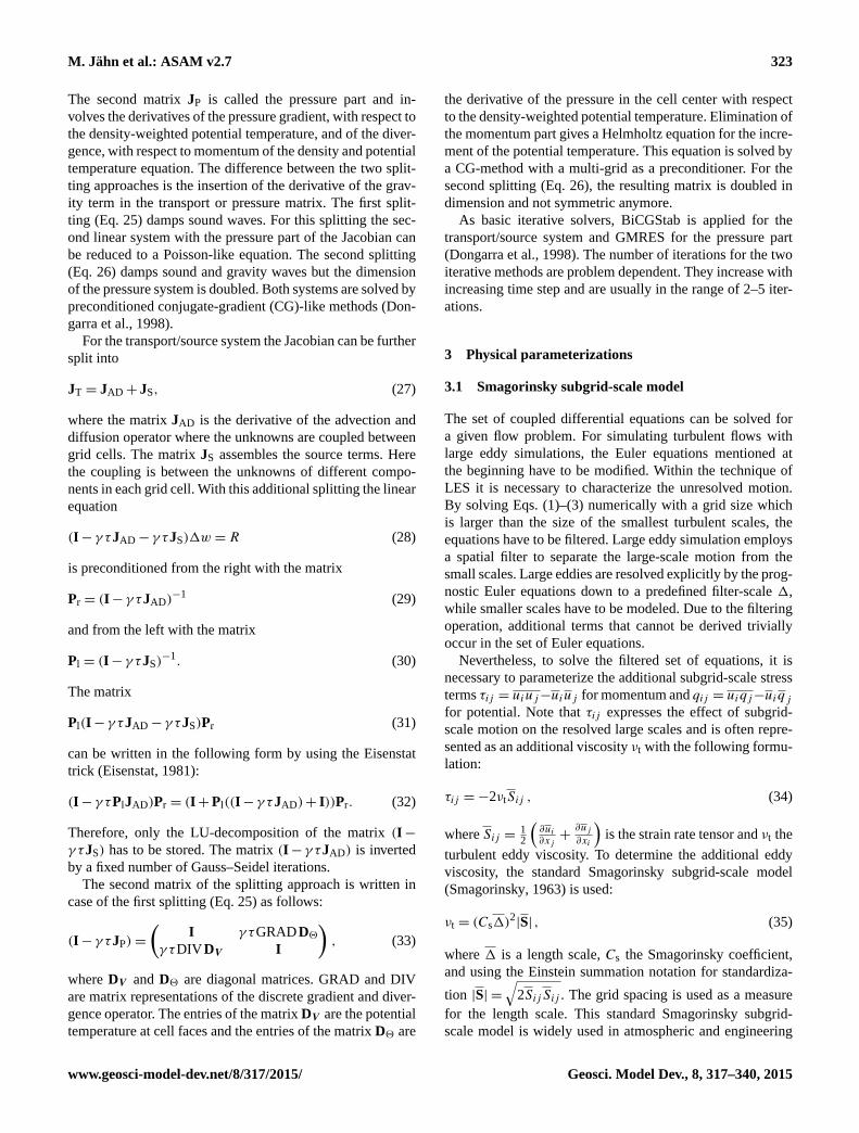
Figure 6. Terminal fall velocity of raindrops after Eq. (56).
58
Figure 6. Terminal fall velocity of raindrops after Eq. (56).
Sk2 = τF
(yn+
2
3k1
)−
4
3k1 , (21)
yn+1 = yn+5
4k1+
3
4k2 , (22)
S= I− γ τJ, J≈ F ′(yn) , (23)
with γ = 12+
16
√3 or in matrix form in Table 2.
Moreover, a new Rosenbrock method was constructed
from a low storage three-stage second-order Runge–Kutta
method, which is used in split-explicit time integration meth-
ods in the Weather Research and Forecasting (WRF) Model
(Skamarock et al., 2008) or in the Consortium for Small-
scale Modeling (COSMO) model (Doms et al., 2011). Its co-
efficients are given in Table 3.
The previously described Rosenbrock W methods allow
a simplified solution of the linear systems without losing the
order. When J= JA+JB the matrix S can be replaced by S=
(I−γ τJA)(I−γ τJB). Further simplification can be reached
by omitting some parts of the Jacobian or by replacing of the
derivatives by the same derivatives of a simplified operator
F (wn). For instance, higher-order interpolation formulae are
replaced by the first-order upwind method. The structure of
the Jacobian is
J=
∂Fρ∂ρ
∂Fρ∂V
0∂FV∂ρ
∂FV∂V
∂FV∂2
0 ∂F2∂V
∂F2∂2
. (24)
A 0 block indicates that this block is not included in the Ja-
cobian or is absent. The derivative with respect to ρ is only
taken for the buoyancy term in the vertical momentum equa-
tion. Note that this type of approximation is the standard
approach in the derivation of the Boussinesq approximation
starting from the compressible Euler equations. The matrix J
can be decomposed as
J= JT+ JP =
∂Fρ∂ρ
0 0∂FV∂ρ
∂FV∂V
0
0 0 ∂F2∂2
+0
∂Fρ∂V
0
0 0∂FV∂2
0 ∂F2∂V
0
(25)
or
J= JT+JP =
∂Fρ∂ρ
0 0
0∂FV∂V
0
0 0 ∂F2∂2
+ 0
∂Fρ∂V
0∂FV∂ρ
0∂FV∂2
0 ∂F2∂V
0
.(26)
The first part of the splitting JT is called the transport/source
part and contains the advection, diffusion and source terms
like Coriolis, curvature, buoyancy, latent heat, and so on.
Geosci. Model Dev., 8, 317–340, 2015 www.geosci-model-dev.net/8/317/2015/
M. Jähn et al.: ASAM v2.7 323
The second matrix JP is called the pressure part and in-
volves the derivatives of the pressure gradient, with respect to
the density-weighted potential temperature, and of the diver-
gence, with respect to momentum of the density and potential
temperature equation. The difference between the two split-
ting approaches is the insertion of the derivative of the grav-
ity term in the transport or pressure matrix. The first split-
ting (Eq. 25) damps sound waves. For this splitting the sec-
ond linear system with the pressure part of the Jacobian can
be reduced to a Poisson-like equation. The second splitting
(Eq. 26) damps sound and gravity waves but the dimension
of the pressure system is doubled. Both systems are solved by
preconditioned conjugate-gradient (CG)-like methods (Don-
garra et al., 1998).
For the transport/source system the Jacobian can be further
split into
JT = JAD+ JS, (27)
where the matrix JAD is the derivative of the advection and
diffusion operator where the unknowns are coupled between
grid cells. The matrix JS assembles the source terms. Here
the coupling is between the unknowns of different compo-
nents in each grid cell. With this additional splitting the linear
equation
(I− γ τJAD− γ τJS)1w = R (28)
is preconditioned from the right with the matrix
Pr = (I− γ τJAD)−1 (29)
and from the left with the matrix
Pl = (I− γ τJS)−1. (30)
The matrix
Pl(I− γ τJAD− γ τJS)Pr (31)
can be written in the following form by using the Eisenstat
trick (Eisenstat, 1981):
(I− γ τPlJAD)Pr = (I+Pl((I− γ τJAD)+ I))Pr. (32)
Therefore, only the LU-decomposition of the matrix (I−
γ τJS) has to be stored. The matrix (I− γ τJAD) is inverted
by a fixed number of Gauss–Seidel iterations.
The second matrix of the splitting approach is written in
case of the first splitting (Eq. 25) as follows:
(I− γ τJP)=
(I γ τGRADD2
γ τDIV DV I
), (33)
where DV and D2 are diagonal matrices. GRAD and DIV
are matrix representations of the discrete gradient and diver-
gence operator. The entries of the matrix DV are the potential
temperature at cell faces and the entries of the matrix D2 are
the derivative of the pressure in the cell center with respect
to the density-weighted potential temperature. Elimination of
the momentum part gives a Helmholtz equation for the incre-
ment of the potential temperature. This equation is solved by
a CG-method with a multi-grid as a preconditioner. For the
second splitting (Eq. 26), the resulting matrix is doubled in
dimension and not symmetric anymore.
As basic iterative solvers, BiCGStab is applied for the
transport/source system and GMRES for the pressure part
(Dongarra et al., 1998). The number of iterations for the two
iterative methods are problem dependent. They increase with
increasing time step and are usually in the range of 2–5 iter-
ations.
3 Physical parameterizations
3.1 Smagorinsky subgrid-scale model
The set of coupled differential equations can be solved for
a given flow problem. For simulating turbulent flows with
large eddy simulations, the Euler equations mentioned at
the beginning have to be modified. Within the technique of
LES it is necessary to characterize the unresolved motion.
By solving Eqs. (1)–(3) numerically with a grid size which
is larger than the size of the smallest turbulent scales, the
equations have to be filtered. Large eddy simulation employs
a spatial filter to separate the large-scale motion from the
small scales. Large eddies are resolved explicitly by the prog-
nostic Euler equations down to a predefined filter-scale 1,
while smaller scales have to be modeled. Due to the filtering
operation, additional terms that cannot be derived trivially
occur in the set of Euler equations.
Nevertheless, to solve the filtered set of equations, it is
necessary to parameterize the additional subgrid-scale stress
terms τij = uiuj−uiuj for momentum and qij = uiqj−uiqjfor potential. Note that τij expresses the effect of subgrid-
scale motion on the resolved large scales and is often repre-
sented as an additional viscosity νt with the following formu-
lation:
τij =−2νtSij , (34)
where Sij =12
(∂ui∂xj+∂uj∂xi
)is the strain rate tensor and νt the
turbulent eddy viscosity. To determine the additional eddy
viscosity, the standard Smagorinsky subgrid-scale model
(Smagorinsky, 1963) is used:
νt = (Cs1)2|S| , (35)
where 1 is a length scale, Cs the Smagorinsky coefficient,
and using the Einstein summation notation for standardiza-
tion |S| =
√2SijSij . The grid spacing is used as a measure
for the length scale. This standard Smagorinsky subgrid-
scale model is widely used in atmospheric and engineering
www.geosci-model-dev.net/8/317/2015/ Geosci. Model Dev., 8, 317–340, 2015
324 M. Jähn et al.: ASAM v2.7
applications. The Smagorinsky coefficient Cs has a theoreti-
cal value of about 0.2, as estimated by Lilly (1967). Applying
this value to a turbulence-driven flow with thermal convec-
tion fields results in a good agreement with observations as
shown by Deardorff (1972).
To take stratification effects into account, Lilly (1962)
modified the standard Smagorinsky formulation by changing
the eddy viscosity to
νt = (Cs1)2max
[0,
(|S|2
(1−
Ri
Pr
))]1/2
(36)
with
Ri=
gθρ
∂θρ∂z
|S|2. (37)
Here, Ri is the Richardson number and Pr is the turbulent
Prandtl number. In a stable boundary layer the vertical gra-
dient of the potential temperature is greater than zero (posi-
tive), which leads to a positive Richardson number and, thus,
the additional term Ri/Pr reduces the square of the strain rate
tensor and decreases the turbulent eddy viscosity. Therefore,
less turbulent vertical mixing takes place.
The implementation in the ASAM code is accomplished
in the main diffusion routine of the model. It develops the
whole term of ∂/∂xj[ρDSij
]for every time step. The coef-
ficient D represents Dmom for the momentum and Dpot for
the potential subgrid-scale stress. Further routines describe
the computation of Dmom and Dpot in the following way:
Dmom = (Cs1)2|S| . (38)
The potential subgrid-scale stress is related to the Prandtl
similarity and can be developed by dividing the subgrid-scale
stress tensor for momentum by the turbulent Prandtl number
Pr that typically has a value of 1/3 (Deardorff, 1972). The
length scale1 in the standard Smagorinsky formulation is set
to the value of grid spacing. However, the cut cell approach
makes it difficult because of tiny and/or anisotropic cells. To
overcome this deficit the value is defined after Scotti et al.
(1993):
1= (111213)1/3f (a1,a2) . (39)
1 is the grid spacing in orthogonal directions, and a correc-
tion function f is applied as follows:
f (a1,a2)= cosh
[4
27
(ln2a1− lna1 lna2+ ln2a2
)]1/2
with a1 =11
13
, a2 =12
13
. (40)
Here, a1 and a2 are the ratios of grid spacing in different
directions with the assumption that 11 ≤12 ≤13. For an
isotropic grid f = 1.
3.2 Two-moment warm cloud microphysics scheme
The implemented microphysics scheme is based on the work
of Seifert and Beheng (2006). This scheme explicitly rep-
resents two moments (mass and number density) of the hy-
drometeor classes cloud droplets and rain drops. Ice phase
hydrometeors are currently not implemented in the model.
Altogether, seven microphysical processes are included: con-
densation/evaporation (COND), cloud condensation nuclei
(CCN) activation to cloud droplets at supersaturated con-
ditions (ACT), autoconversion (AUTO), self-collection of
cloud droplets (SCC), self-collection of rain drops (SCR),
accretion (ACC) and evaporation of rain (EVAP):
∂(ρqv)
∂t+∇ · (ρvqv)=−SCOND− SACT+ SEVAP , (41)
∂(ρqc)
∂t+∇ · (ρvqc)=+SCOND+ SACT− SAUTO− SACC , (42)
∂(ρqr)
∂t+∇ · (ρvqr)=+SAUTO+ SACC− SEVAP , (43)
∂NCCN
∂t+∇ · (vNCCN)=−SCONDN − SACTN + SEVAPN , (44)
∂Nc
∂t+∇ · (vNc)=+SCONDN + SACTN − SAUTON
− SACCN − SSCC , (45)
∂Nr
∂t+∇ · (vNr)=+SAUTON + SACCN − SEVAPN − SSCR . (46)
Details on the conversion rates can be found in Seifert and
Beheng (2006). Additionally, a limiter function is used to
ensure numerical stability and avoid nonphysical negative
values (Horn, 2012). Since there is no saturation adjustment
technique in ASAM, the condensation process is taken as an
example to demonstrate the physical meaning of the limiter
functions. Considering the available water vapor density ρv
and the cloud water density ρc, the process of condensation
(or evaporation of cloud water, respectively) is forced by the
water vapor density deficit and limited by the available cloud
water.
FOR= ρv− (pvsT/Rv) (47)
LIM= ρc (48)
SCOND =FOR−LIM+ (FOR2
+LIM2)1/2
τCOND
(49)
Here, pvs is the saturation vapor pressure and the relaxation
time is set to τCOND = 1 s. The numerator term is called the
Fischer–Burmeister function and has originally been used in
the optimization of complementary problems (cf. Kong et al.,
2010). A simple model after Horn (2012) is applied to deter-
mine the corresponding changes in the number concentra-
tions and to ensure a reduction of the cloud droplet number
density to zero if there is no cloud water present. This means
that Nc decreases when droplets are getting too small,
SCONDN =min
(0,C
[ρc
xmin
−Nc
]), (50)
Geosci. Model Dev., 8, 317–340, 2015 www.geosci-model-dev.net/8/317/2015/
M. Jähn et al.: ASAM v2.7 325
and increases when droplets are getting too large,
SCONDN =max
(0,C
[ρc
xmax
−Nc
]), (51)
where xmin and xmax are limiting parameters for cloud wa-
ter. This ensures that the cloud droplet number concentra-
tion is within a certain range defined by distribution param-
eters in Seifert and Beheng (2006) if condensate is present.
A timescale factor of C = 0.01 s−1 controls the speed of this
correction and appears to be reasonable for this particular
process.
3.3 Precipitation
The sedimentation velocity of raindrops is derived as in
the operationally used COSMO model from the German
Weather Service (Doms et al., 2011). There, the following
assumptions are made. The precipitation particles are ex-
ponentially distributed with respect to their drop diameter
(Marshall–Palmer distribution):
fr(D)=Nr0 exp−λrD. (52)
Here, λr is the slope parameter of the distribution function
and N r0 = 8× 10⁶ m−4 is an empirically determined distri-
bution parameter. The terminal fall velocity of raindrops is
then assumed to be uniquely related to drop size, which is
expressed by the following empirical function:
Wf(D)= crD1/2 (53)
with cr = 130m1/2 s−1. Finally, the precipitation flux of rain-
water can be calculated as
Pr = ρrWf(ρr)=
∞∫0
m(D)Wf(D)fr(D)dD (54)
with the raindrop mass
m(D)= πρWD3/6 , (55)
where ρW = 1000kgm−3 is the mass density of water. This
leads to an expression for the terminal fall velocity of rain-
drops in dependence on their density:
Wf(ρr)=−cr
0(4,5)
6
(ρr
πρWN0r
)1/8
. (56)
This takes place at the tendency equation for the rain water
density:
∂(ρqr)
∂t+∇h · (ρvhqr)+
∂
∂z(ρqr [w+Wf])= Sqr . (57)
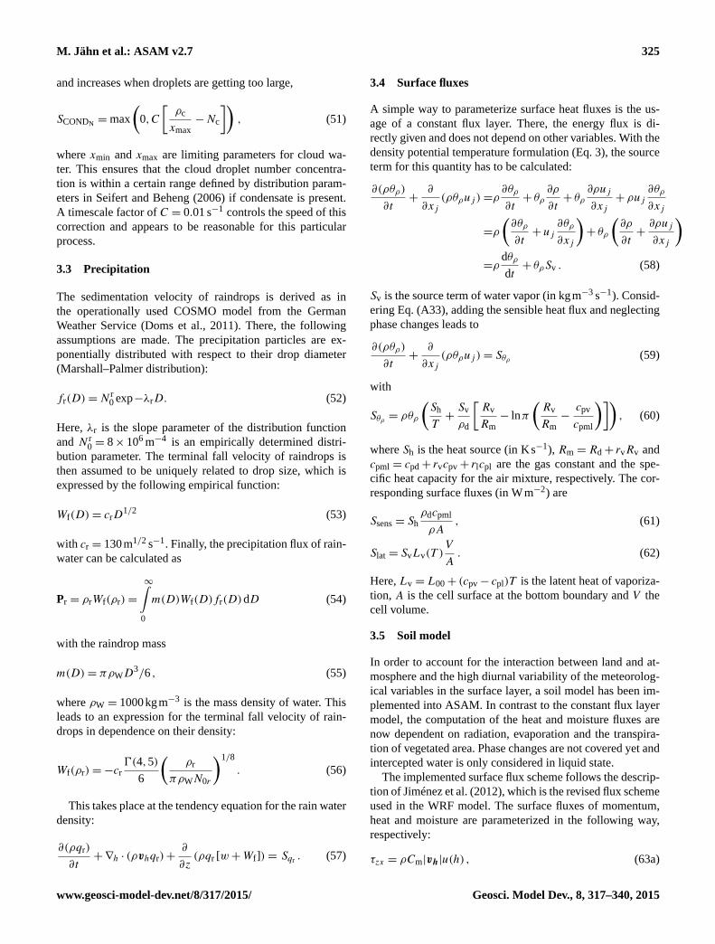
3.4 Surface fluxes
A simple way to parameterize surface heat fluxes is the us-
age of a constant flux layer. There, the energy flux is di-
rectly given and does not depend on other variables. With the
density potential temperature formulation (Eq. 3), the source
term for this quantity has to be calculated:
∂(ρθρ)
∂t+
∂
∂xj(ρθρuj )=ρ
∂θρ
∂t+ θρ
∂ρ
∂t+ θρ
∂ρuj
∂xj+ ρuj
∂θρ
∂xj
=ρ
(∂θρ
∂t+ uj
∂θρ
∂xj
)+ θρ
(∂ρ
∂t+∂ρuj
∂xj
)=ρ
dθρ
dt+ θρSv . (58)
Sv is the source term of water vapor (in kgm−3 s−1). Consid-
ering Eq. (A33), adding the sensible heat flux and neglecting
phase changes leads to
∂(ρθρ)
∂t+
∂
∂xj(ρθρuj )= Sθρ (59)
with
Sθρ = ρθρ
(Sh
T+Sv
ρd
[Rv
Rm
− lnπ
(Rv
Rm
−cpv
cpml
)]), (60)
where Sh is the heat source (in Ks−1), Rm = Rd+ rvRv and
cpml = cpd+ rvcpv+ rlcpl are the gas constant and the spe-
cific heat capacity for the air mixture, respectively. The cor-
responding surface fluxes (in Wm−2) are
Ssens = Sh
ρdcpml
ρA, (61)
Slat = SvLv(T )V
A. (62)
Here, Lv = L00+ (cpv− cpl)T is the latent heat of vaporiza-
tion, A is the cell surface at the bottom boundary and V the
cell volume.
3.5 Soil model
In order to account for the interaction between land and at-
mosphere and the high diurnal variability of the meteorolog-
ical variables in the surface layer, a soil model has been im-
plemented into ASAM. In contrast to the constant flux layer
model, the computation of the heat and moisture fluxes are
now dependent on radiation, evaporation and the transpira-
tion of vegetated area. Phase changes are not covered yet and
intercepted water is only considered in liquid state.
The implemented surface flux scheme follows the descrip-
tion of Jiménez et al. (2012), which is the revised flux scheme
used in the WRF model. The surface fluxes of momentum,
heat and moisture are parameterized in the following way,
respectively:
τzx = ρCm|vh|u(h) , (63a)
www.geosci-model-dev.net/8/317/2015/ Geosci. Model Dev., 8, 317–340, 2015

326 M. Jähn et al.: ASAM v2.7
− ρcpw′θ ′ = ρcpCh|vh|(θ(h)− θ(z0T )) , (63b)
− ρLw′q ′ = ρLCq|vh|(q(h)− q(z0q)
). (63c)
Cm, Ch and Cq are the bulk transfer coefficients and it is con-
sidered that Ch = Cq. In Jiménez et al. (2012), the bulk trans-
fer coefficients are defined as follows:
Cm, h =k2
9M9M, H
(64)
with
9M ,H = ln
(z+ z0
z0
)−φm, h
(z+ z0
L
)+φm, h
(z0
L
)(65)
and φm, h representing the integrated similarity functions. L
stands for the Obukhov length and k is the von Kármán
constant. In neutral to highly stable conditions φm, h follows
Cheng and Brutsaert (2005) and in unstable situations the φ-
functions follow Fairall et al. (1996). For further details con-
cerning limitations and restrictions see Jiménez et al. (2012).
The transport of the soil water as a result of hydraulic pres-
sure due to diffusion and gravity within the soil layers is de-
scribed by Richard’s equation:
∂Wsoil,k
∂t=∂
∂z
(Diff
∂Wsoil,k
∂z+ κsoil,k
)(66)
with the diffusion coefficient
Diff = κsoil,k
∂9soil,k
∂Wsoil,k
. (67)
Wsoil,k is the volumetric water content in the kth soil layer.
9soil stands for the matric potential and κsoil is the hy-
draulic conductivity. 9soil and κsoil are parameterized based
on Van Genuchten (1980):
κsoil = κsat
√Weff
(1−
[1− (Weff)
1m
]m)2′
(68)
9soil =9sat
[(Weff)
−1m − 1
] 1n. (69)
Weff describes the effective soil wetness, which takes a resid-
ual water content Wres into account, restricting the soil from
complete desiccation. κsat and 9sat are the hydraulic conduc-
tivity and the matric potential at saturated conditions, respec-
tively. The parameters m and n describe the pore distribution
(Braun, 2002) withm= 1−1/n (also see Tables B1 and B2).
Further addition/extraction of soil water is controlled by
the percolation of intercepted water into the ground and the
evaporation and transpiration of water from bare soil and
vegetation. The mechanisms implemented are based on the
Multi-Layer Soil and Vegetation Model TERRA_ML as de-
scribed in Doms et al. (2011). The evaporation of bare soil
is adjusted to the parameterization proposed by Noilhan and
Planton (1989). The variation of the soil temperature is a re-
sult of heat conductivity depending on the soil texture and
the soil water content of the respective soil layer:
∂Tsoil
∂t=
1
ρc
∂
∂z
[λ∂Tsoil
∂z+EqρwcwT soil
]. (70)
Tsoil is the absolute temperature in the kth soil layer (in K),
T soil is the mean soil temperature of two neighboring soil
layers. The change in internal energy due to changes in mois-
ture by the inner soil water flux, evapotranspiration and evap-
oration from the upper soil layer and the interception reser-
voir is treated by the second term in brackets. The heat con-
ductivity λ and the volumetric heat capacity ρc are variables
that depend on the soil texture. The heat capacity of the soil
ρc formulated by Chen and Dudhia (2001) is the sum of the
heat capacity of dry soil (ρ0c0, see Tables B1 and B2), the
heat capacity of wet soil (ρwcw) and the heat capacity of the
air within the soil pores (ρaca).
ρc =Wsoilρwcw+(1−Wpv
)ρ0c0+
(Wpv−Wsoil
)ρaca (71)
with Wpv corresponding to the soil pores, ρwcw = 4.18×
106 Jm−3 K−1 and ρaca = 1298 Jm−3 K−1. The heat con-
ductivity λ is defined after Pielke (1984):
λ=
{418exp
{−9log− 2.7
}if 9log ≤ 5.1
0.172 if 9log > 5.1(72)
with 9log = log10 |1009soil|.
The topmost layer is exposed to the incoming radiation
and thus has the strongest variation in temperature in com-
parison to the other soil layers within the ground. The tem-
perature equation of the first layer is, in addition to the in-
coming radiation, determined by the latent and sensible heat
flux.
∂Tsoil,1
∂t=
1
ρc
∂
∂z
[(λ∂Tsoil,1
∂z
)+1Q
](73)
with
1Q=Qdir+Qdif− σT4
sfc− cpQSH−LvQLH. (74)
Here,QLH is the latent heat flux, describing the moisture flux
between soil and atmosphere as the sum of evaporation and
transpiration andQSH is the sensible heat flux.Qdir andQdif
represent the direct and diffusive irradiation, respectively.
4 Test cases
In this section, we present six example test cases. In five of
these cases, orography or obstacles are included to test con-
servation properties and model accuracy. The first test case is
the rising heat bubble prescribed in Wicker and Skamarock
Geosci. Model Dev., 8, 317–340, 2015 www.geosci-model-dev.net/8/317/2015/
M. Jähn et al.: ASAM v2.7 327
Discussion
Paper
|D
iscussionPaper
|D
iscussionPaper
|D
iscussionPaper
|
0 0-2 -2-4 -4-6 -62 24 46 60
2
4
6
8
10
Figure 7. Results for the dry bubble simulation after Wicker and Skamarock (1998) at t= 1000 s:contours of perturbation potential temperature (left panel) and vertical velocity (right panel). Solid(dashed) lines indicate positive (negative) values. Contour intervals are 0.25 K (zero contour omitted)and 2 m s−1, respectively.
59
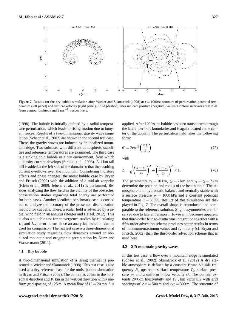
Figure 7. Results for the dry bubble simulation after Wicker and Skamarock (1998) at t = 1000 s: contours of perturbation potential tem-
perature (left panel) and vertical velocity (right panel). Solid (dashed) lines indicate positive (negative) values. Contour intervals are 0.25 K
(zero contour omitted) and 2 ms−1, respectively.
(1998). The bubble is initially defined by a radial tempera-
ture perturbation, which leads to rising motion due to buoy-
ant forces. Results of a two-dimensional gravity wave simu-
lation (Schaer et al., 2002) are shown in the second test case.
There, the gravity waves are induced by an idealized moun-
tain ridge. Two subcases with different atmospheric stabili-
ties and reference temperatures are examined. The third case
is a sinking cold bubble in a dry environment, from which
a density current develops (Straka et al., 1993). A 1 km tall
hill is added at the left side of the domain so that the resulting
current overflows over the mountain. Considering moisture
effects and phase changes, the moist bubble case by Bryan
and Fritsch (2002) with the addition of a mid-air zeppelin
(Klein et al., 2009; Jebens et al., 2011) is performed. Be-
sides analyzing the flow field in the vicinity of the obstacles,
conservation studies regarding total energy are performed
for both cases. Another idealized benchmark case is carried
out to analyze the accuracy of the presented discretization
method for cut cells. There, a scalar field is advected by a ra-
dial wind field in an annulus (Berger and Helzel, 2012). This
is also a suitable test for convergence studies by calculating
L1 and L∞ error norms since an analytical solution can be
used for comparison. The last test case is a three-dimensional
simulation study regarding flow dynamics around an ide-
alized mountain and orographic precipitation by Kunz and
Wassermann (2011).
4.1 Dry bubble
A two-dimensional simulation of a rising thermal is pre-
sented in Wicker and Skamarock (1998). This test case is also
used as a dry reference case for the moist bubble simulation
in Bryan and Fritsch (2002). The domain is 20 km in the hori-
zontal direction and 10 km in the vertical direction with a uni-
form grid spacing of 125 m. A mean flow of U = 20 ms−1 is
applied. After 1000 s the bubble has been transported through
the lateral periodic boundaries and is again located at the cen-
ter of the domain. The perturbation field takes the following
form:
θ ′ = 2cos2
(πL
2
)(75)
with
L=
√(x− xc
xr
)2
+
(z− zc
zr
)2
≤ 1 . (76)
The parameters xc = 10 km, zc = 2 km and xr = zr = 2 km
determine the position and radius of the heat bubble. The at-
mosphere is in hydrostatic balance and neutrally stable with
a surface pressure p0 = 1000 hPa and a constant potential
temperature θ = 300 K. Results of this simulation are dis-
played in Fig. 7. The overall shape is reproduced and com-
parable to the reference solution. Slight asymmetries are ob-
served due to lateral transport. However, it becomes apparent
that third-order Runge–Kutta time integration together with a
fifth-order advection scheme produces better results in terms
of minimum/maximum values and symmetry (cf. Bryan and
Fritsch, 2002) than the third-order advection scheme that is
used here.
4.2 2-D mountain gravity waves
In this test case, a flow over a mountain ridge is simulated
(Schaer et al., 2002). Skamarock et al. (2012) A dry sta-
ble atmosphere is defined by a constant Brunt–Väisälä fre-
quency N , upstream surface temperature T0, surface pres-
sure p0 and a uniform inflow velocity U . The domain ex-
tends 200 km horizontally and 19.5 km vertically with grid
spacings of 1x = 500 m and 1z= 300 m. The structure of
www.geosci-model-dev.net/8/317/2015/ Geosci. Model Dev., 8, 317–340, 2015
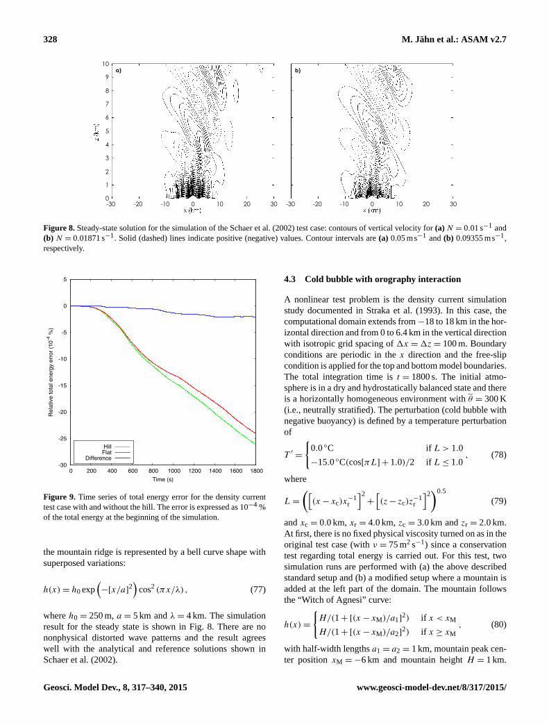
328 M. Jähn et al.: ASAM v2.7
Discussion
Paper
|D
iscussionPaper
|D
iscussionPaper
|D
iscussionPaper
|
a) b)
0 0-10 -10-20-20-30 -3010 1020 2030 300
1
2
3
4
5
6
7
8
9
10
Figure 8. Steady-state solution for the simulation of the Schaer et al. (2002) test case: contours ofvertical velocity for a) N = 0.01 s−1 and b) N = 0.01871 s−1. Solid (dashed) lines indicate positive(negative) values. Contour intervals are a) 0.05 m s−1 and b) 0.09355 m s−1, respectively.
60
Figure 8. Steady-state solution for the simulation of the Schaer et al. (2002) test case: contours of vertical velocity for (a) N = 0.01 s−1 and
(b) N = 0.01871 s−1. Solid (dashed) lines indicate positive (negative) values. Contour intervals are (a) 0.05 ms−1 and (b) 0.09355 ms−1,
respectively.D
iscussionPaper
|D
iscussionPaper
|D
iscussionPaper
|D
iscussionPaper
|
-30
-25
-20
-15
-10
-5
0
5
0 200 400 600 800 1000 1200 1400 1600 1800
Rel
ativ
e to
tal e
nerg
y er
ror (
10-4
%)
Time (s)
HillFlat
Difference
Figure 9. Time series of total energy error for the density current test case with and without the hill.The error is expressed as 10−4 % of the total energy at the beginning of the simulation.
61
Figure 9. Time series of total energy error for the density current
test case with and without the hill. The error is expressed as 10−4 %
of the total energy at the beginning of the simulation.
the mountain ridge is represented by a bell curve shape with
superposed variations:
h(x)= h0 exp(−[x/a]2
)cos2 (πx/λ), (77)
where h0 = 250 m, a = 5 km and λ= 4 km. The simulation
result for the steady state is shown in Fig. 8. There are no
nonphysical distorted wave patterns and the result agrees
well with the analytical and reference solutions shown in
Schaer et al. (2002).
4.3 Cold bubble with orography interaction
A nonlinear test problem is the density current simulation
study documented in Straka et al. (1993). In this case, the
computational domain extends from−18 to 18 km in the hor-
izontal direction and from 0 to 6.4 km in the vertical direction
with isotropic grid spacing of 1x =1z= 100 m. Boundary
conditions are periodic in the x direction and the free-slip
condition is applied for the top and bottom model boundaries.
The total integration time is t = 1800 s. The initial atmo-
sphere is in a dry and hydrostatically balanced state and there
is a horizontally homogeneous environment with θ = 300 K
(i.e., neutrally stratified). The perturbation (cold bubble with
negative buoyancy) is defined by a temperature perturbation
of
T ′ =
{0.0 ◦C if L > 1.0
−15.0 ◦C(cos[πL] + 1.0)/2 if L≤ 1.0, (78)
where
L=
([(x− xc)x
−1r
]2
+
[(z− zc)z
−1r
]2)0.5
(79)
and xc = 0.0 km, xr = 4.0 km, zc = 3.0 km and zr = 2.0 km.
At first, there is no fixed physical viscosity turned on as in the
original test case (with ν = 75 m2 s−1) since a conservation
test regarding total energy is carried out. For this test, two
simulation runs are performed with (a) the above described
standard setup and (b) a modified setup where a mountain is
added at the left part of the domain. The mountain follows
the “Witch of Agnesi” curve:
h(x)=
{H/(1+ [(x− xM)/a1]
2) if x < xM
H/(1+ [(x− xM)/a2]2) if x ≥ xM
, (80)
with half-width lengths a1 = a2 = 1 km, mountain peak cen-
ter position xM =−6 km and mountain height H = 1 km.
Geosci. Model Dev., 8, 317–340, 2015 www.geosci-model-dev.net/8/317/2015/
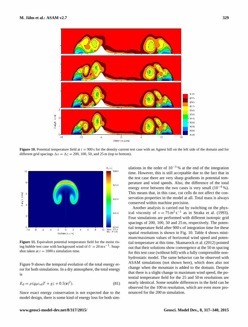
M. Jähn et al.: ASAM v2.7 329
Discussion
Paper
|D
iscussionPaper
|D
iscussionPaper
|D
iscussionPaper
|
0-6-12-18 6 12 180
1
2
3
Figure 10. Potential temperature field at t = 900 s for the density current test case with an ’Agnesi’hill on the left side of the domain and for different grid spacings ∆x= ∆z = 200, 100, 50, 25 m (topto bottom).
62
Figure 10. Potential temperature field at t = 900 s for the density current test case with an Agnesi hill on the left side of the domain and for
different grid spacings 1x =1z= 200, 100, 50, and 25 m (top to bottom).
Discussion
Paper
|D
iscussionPaper
|D
iscussionPaper
|D
iscussionPaper
|
0 2 4 6 8 10-2-4-6-8-100
2
4
6
8
10
Figure 11. Equivalent potential temperature field for the moist rising bubble test case with back-ground wind of U = 20 m s−1. Snapshot taken at t= 1000 s simulation time.
63
Figure 11. Equivalent potential temperature field for the moist ris-
ing bubble test case with background wind of U = 20 ms−1. Snap-
shot taken at t = 1000 s simulation time.
Figure 9 shows the temporal evolution of the total energy er-
ror for both simulations. In a dry atmosphere, the total energy
is
Ed = ρ(qdcvdT + gz+ 0.5|v|2). (81)
Since exact energy conservation is not expected due to the
model design, there is some kind of energy loss for both sim-
ulations in the order of 10−3 % at the end of the integration
time. However, this is still acceptable due to the fact that in
the test case there are very sharp gradients in potential tem-
perature and wind speeds. Also, the difference of the total
energy error between the two cases is very small (10−4 %).
This means that, in this case, cut cells do not affect the con-
servation properties in the model at all. Total mass is always
conserved within machine precision.
Another analysis is carried out by switching on the phys-
ical viscosity of ν = 75 m2 s−1 as in Straka et al. (1993).
Four simulations are performed with different isotropic grid
spacings of 200, 100, 50 and 25 m, respectively. The poten-
tial temperature field after 900 s of integration time for these
spatial resolutions is shown in Fig. 10. Table 4 shows mini-
mum/maximum values of horizontal wind speed and poten-
tial temperature at this time. Skamarock et al. (2012) pointed
out that their solutions show convergence at the 50 m spacing
for this test case (without hill) with a fully compressible non-
hydrostatic model. The same behavior can be observed with
ASAM simulations (not shown here), which does also not
change when the mountain is added to the domain. Despite
that there is a slight change in maximum wind speed, the po-
tential temperature field for the 25 and 50 m resolutions are
nearly identical. Some notable differences in the field can be
observed for the 100 m resolution, which are even more pro-
nounced for the 200 m simulation.
www.geosci-model-dev.net/8/317/2015/ Geosci. Model Dev., 8, 317–340, 2015
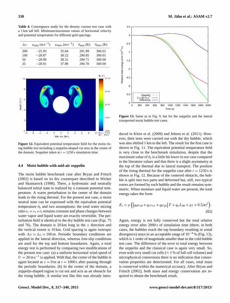
330 M. Jähn et al.: ASAM v2.7
Table 4. Convergence study for the density current test case with
a 1 km tall hill. Minimum/maximum values of horizontal velocity
and potential temperature for different grid spacings.
1x umin (ms−1) umax (ms−1) θmin (K) θmax (K)
200 −25.93 35.64 291.89 300.01
100 −28.87 38.52 290.85 300.01
50 −28.90 38.31 290.71 300.00
25 −28.91 37.89 290.70 300.00
Discussion
Paper
|D
iscussionPaper
|D
iscussionPaper
|D
iscussionPaper
|
0 2 4 6 8 10-2-4-6-8-100
2
4
6
8
10
Figure 12. Equivalent potential temperature field for the moist rising bubble test including a zeppelin-shaped cut area in the center of the domain. Snapshot taken at t= 1250 s simulation time.
64
Figure 12. Equivalent potential temperature field for the moist ris-
ing bubble test including a zeppelin-shaped cut area in the center of
the domain. Snapshot taken at t = 1250 s simulation time.
4.4 Moist bubble with mid-air zeppelin
The moist bubble benchmark case after Bryan and Fritsch
(2002) is based on its dry counterpart described in Wicker
and Skamarock (1998). There, a hydrostatic and neutrally
balanced initial state is realized by a constant potential tem-
perature. A warm perturbation in the center of the domain
leads to the rising thermal. For the present test case, a moist
neutral state can be expressed with the equivalent potential
temperature θe and two assumptions: the total water mixing
ratio rt = rv+rl remains constant and phase changes between
water vapor and liquid water are exactly reversible. The per-
turbation field is identical to the dry bubble test case (Eqs. 75
and 76). The domain is 20 km long in the x direction and
the vertical extent is 10 km. Grid spacing is again isotropic
with 1x =1z= 100 m. Periodic boundary conditions are
applied in the lateral direction, whereas free-slip conditions
are used for the top and bottom boundaries. Again, a total
energy test is performed by comparing two modifications of
the present test case: (a) a uniform horizontal wind speed of
U = 20 ms−1 is applied. With that, the center of the bubble is
again located at x = 0 m at t = 1000 s after passing through
the periodic boundaries. (b) In the center of the domain, a
zeppelin-shaped region is cut out and acts as an obstacle for
the rising bubble. A similar test like this was already intro-
Discussion
Paper
|D
iscussionPaper
|D
iscussionPaper
|D
iscussionPaper
|
-4
-3.5
-3
-2.5
-2
-1.5
-1
-0.5
0
0.5
0 200 400 600 800 1000 1200 1400 1600 1800 2000
Rel
ativ
e to
tal e
nerg
y er
ror (
10-4
%)
Time (s)
ZeppelinU = 20 m s-1
Difference
Figure 13. Same as Fig. 9, but for the zeppelin and the lateral transported moist bubble test cases.
65
Figure 13. Same as in Fig. 9, but for the zeppelin and the lateral
transported moist bubble test cases.
duced in Klein et al. (2009) and Jebens et al. (2011). How-
ever, their tests were carried out with the dry bubble, which
was also shifted 1 km to the left. The result for the first case is
shown in Fig. 11. The equivalent potential temperature field
is very close to the benchmark simulation, despite that the
maximum value of θe is a little bit lower in our case compared
to the literature values and that there is a slight asymmetry at
the top of the thermal due to lateral transport. The position
of the rising thermal for the zeppelin case after t = 1250 s is
shown in Fig. 12. Because of the centered obstacle, the bub-
ble is split into two parts and deformed but, still, two typical
rotors are formed by each bubble and the result remains sym-
metric. When moisture and liquid water are present, the total
energy takes the form
Et = ρ([qdcvd+ qvcvv+ qlcpl
]T + qvL00+ gz+ 0.5|v|2
).
(82)
Again, energy is not fully conserved but the total relative
energy error after 2000 s of simulation time (there, in both
cases, the bubbles reach the top boundary resulting in zonal
divergence) stays in an acceptable range of 10−4 % (Fig. 13),
which is 1 order of magnitude smaller than in the cold bubble
test case. The difference of the error in total energy between
the zeppelin and the classical case is again very small. So,
even with very small cut cells (≈ 1 % of full cell volume) and
microphysical conversions there is no indication that conser-
vation properties are deteriorated. For all cases, total mass
is conserved within the numerical accuracy. After Bryan and
Fritsch (2002), both mass and energy conservation are re-
quired to obtain the benchmark result.
Geosci. Model Dev., 8, 317–340, 2015 www.geosci-model-dev.net/8/317/2015/
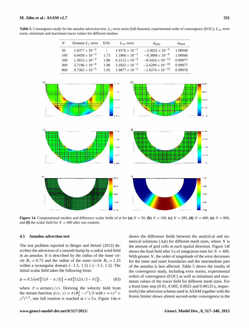
M. Jähn et al.: ASAM v2.7 331
Table 5. Convergence study for the annulus advection test. L1 error norm (full domain), experimental order of convergence (EOC), L∞ error
norm, minimum and maximum tracer values for different meshes.
N Domain L1 error EOC L∞ error φmin φmax
50 1.6377× 10⁻² – 1.9176× 10⁻¹−2.0022× 10⁻³ 1.00048
100 4.9439× 10⁻³ 1.73 1.1860× 10⁻¹−8.3884× 10⁻⁴ 1.00066
200 1.3653× 10⁻³ 1.86 6.3112× 10⁻²−8.5424× 10⁻¹³ 0.99977
400 3.7196× 10⁻⁴ 1.88 3.1822× 10⁻²−2.6209× 10⁻¹⁶ 0.99977
800 9.7302× 10⁻⁵ 1.93 1.9877× 10⁻²−1.0274× 10⁻¹² 0.99978
Discussion
Paper
|D
iscussionPaper
|D
iscussionPaper
|D
iscussionPaper
|
1
Figure 14. Computational meshes and difference scalar fields of φ for a) N = 50, b) N = 100, c)N = 200, d) N = 400, e) N = 800, f) scalar field for N = 400 after one rotation.
66
Figure 14. Computational meshes and difference scalar fields of φ for (a) N = 50, (b) N = 100, (c) N = 200, (d) N = 400, (e) N = 800,
and (f) the scalar field for N = 400 after one rotation.
4.5 Annulus advection test
The test problem reported in Berger and Helzel (2012) de-
scribes the advection of a smooth bump by a radial wind field
in an annulus. It is described by the radius of the inner cir-
cle R1 = 0.75 and the radius of the outer circle R2 = 1.25
within a rectangular domain [−1.5, 1.5]× [−1.5, 1.5]. The
initial scalar field takes the following form:
φ = 0.5(erf[5 {ϑ −π/3}
]+ erf
[5 {2π/3−ϑ}
]), (83)
where ϑ = arctan(y/x). Deriving the velocity field from
the stream function ψ(x,y)= π(R22 − r
2)/5 with r = (x2+
y2)1/2, one full rotation is reached at t = 5 s. Figure 14a–e
shows the difference fields between the analytical and nu-
merical solutions (1φ) for different mesh sizes, where N is
the amount of grid cells in each spatial direction. Figure 14f
shows the final field after 5 s of integration time forN = 400.
With greaterN , the order of magnitude of the error decreases
for the inner and outer boundaries and the intermediate part
of the annulus is less affected. Table 5 shows the results of
the convergence study, including error norms, experimental
orders of convergence (EOC) as well as minimum and max-
imum values of the tracer field for different mesh sizes. For
a fixed time step (0.01, 0.005, 0.0025 and 0.00125 s, respec-
tively) the advection scheme used in ASAM together with the
Koren limiter shows almost second-order convergence in the
www.geosci-model-dev.net/8/317/2015/ Geosci. Model Dev., 8, 317–340, 2015
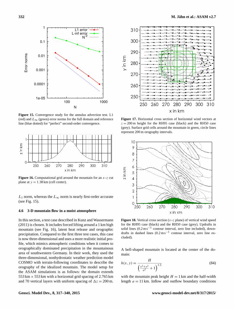
332 M. Jähn et al.: ASAM v2.7
Discussion
Paper
|D
iscussionPaper
|D
iscussionPaper
|D
iscussionPaper
|
1e-05
0.0001
0.001
0.01
0.1
1
100 1000
Err
or
norm
s
N
L1 error
L-inf error
N-2
Figure 15. Convergence study for the annulus advection test. L1 (red) and L-infinity (green) errornorms for the full domain and reference line (blue dotted) for "perfect" 2nd order convergence.
67
Figure 15. Convergence study for the annulus advection test. L1
(red) and L∞ (green) error norms for the full domain and reference
line (blue dotted) for “perfect” second-order convergence.
Discussion
Paper
|D
iscussionPaper
|D
iscussionPaper
|D
iscussionPaper
|
x in km280 290 300 310270260250
0
1
Figure 16. Computational grid around the mountain for an x-z cut plane at y =1.38 km (cell center).
68
Figure 16. Computational grid around the mountain for an x–z cut
plane at y = 1.38 km (cell center).
L1 norm, whereas the L∞ norm is nearly first-order accurate
(see Fig. 15).
4.6 3-D mountain flow in a moist atmosphere
In this section, a test case described in Kunz and Wassermann
(2011) is chosen. It includes forced lifting around a 1 km high
mountain (see Fig. 16), latent heat release and orographic
precipitation. Compared to the first three test cases, this case
is now three-dimensional and uses a more realistic initial pro-
file, which mimics atmospheric conditions when it comes to
orographically dominated precipitation in the mountainous
area of southwestern Germany. In their work, they used the
three-dimensional, nonhydrostatic weather prediction model
COSMO with terrain-following coordinates to describe the
orography of the idealized mountain. The model setup for
the ASAM simulations is as follows: the domain extends
553 km× 553 km with a horizontal grid spacing of 2.765 km
and 70 vertical layers with uniform spacing of 1z= 200 m.
Discussion
Paper
|D
iscussionPaper
|D
iscussionPaper
|D
iscussionPaper
|
x in km280
280
270
270
260
260
250
250
290
290
300
300
310
310
Figure 17. Horizontal cross-section of horizontal wind vectors at z = 200 m height for the RH95case (black) and the RH50 case (grey). Surface grid cells around the mountain in green, circle linesrepresent 200 m orography intervals.
69
Figure 17. Horizontal cross section of horizontal wind vectors at
z= 200 m height for the RH95 case (black) and the RH50 case
(grey). Surface grid cells around the mountain in green, circle lines
represent 200 m orography intervals.
Discussion
Paper
|D
iscussionPaper
|D
iscussionPaper
|D
iscussionPaper
|
Figure 18. Vertical cross-section (x-z plane) of vertical wind speed for the RH95 case (black) and theRH50 case (grey). Updrafts in solid lines (0.2 m s−1 contour interval, zero line included), downdraftsin dashed lines (0.2 m s−1 contour interval, zero line excluded).
70
Figure 18. Vertical cross section (x–z plane) of vertical wind speed
for the RH95 case (black) and the RH50 case (grey). Updrafts in
solid lines (0.2 ms−1 contour interval, zero line included), down-
drafts in dashed lines (0.2 ms−1 contour interval, zero line ex-
cluded).
A bell-shaped mountain is located at the center of the do-
main:
h(x,y)=H(
x2+y2
a2 + 1)1.5
(84)
with the mountain peak height H = 1 km and the half-width
length a = 11 km. Inflow and outflow boundary conditions
Geosci. Model Dev., 8, 317–340, 2015 www.geosci-model-dev.net/8/317/2015/

M. Jähn et al.: ASAM v2.7 333
Discussion
Paper
|D
iscussionPaper
|D
iscussionPaper
|D
iscussionPaper
|
x in km
2802702602500
1
2
3
4
5
6
7
240 290 300 310 320 330 340
qrqcLWC(g/kg) (g/kg) (g/kg)
Figure 19. Vertical cross-section (x-z plane) of microphysical properties for the RH95 case. Liquidwater content (shaded), contours of specific cloud water content qc (red-yellow) and specific rainwater content qr (blue).
71
Figure 19. Vertical cross section (x–z plane) of microphysical properties for the RH95 case. Liquid water content (shaded), contours of
specific cloud water content qc (red–yellow) and specific rain water content qr (blue).
are set according to the initial conditions. A Rayleigh damp-
ing layer above 11 km is applied to suppress gravity wave
reflections from the top boundary. Surface heat fluxes and
Coriolis force are turned off. For turbulence parameteriza-
tion, the standard Smagorinsky subgrid-scale model is used.
Microphysics are parameterized by the warm (i.e., no ice
phase present) two-moment scheme described in Sect. 3.2.
Initial profiles are obtained by assuming hydrostatic equi-
librium, a near-surface temperature Ts = 283.15 K, a con-
stant mean flow U = 10 ms−1, a constant dry static stability
Nd = 11×10−3 s−1 and a relative humidity profile, which is
constant up to zm = 5 km and rapidly decreases above this
level according to
RH(z)= RHS
[0.5+π−1 arctan
(z− zm
500
)](85)
with the near-surface humidity RHS = 95 % (RH95 case). To
compare the results with its dry counterpart, another simula-
tion with RHS = 50 % is performed (RH50 case). Figure 17
shows the wind field at 200 m height around the mountain
for both cases. In the nearly saturated atmosphere, there is
a more direct overflow over the mountain, which is caused
by the reduced stability due to high moisture. These dif-
ferent flow characteristics also affect gravity wave structure
(Fig. 18). The resulting waves are steeper and have a greater
wavelength, which is in agreement with gravity wave theory
and the results from Kunz and Wassermann (2011). Most no-
table differences in the numerical results are discrepancies in
vertical wind strength in the lowest model layer at the wind-
ward side the mountain (w ≈ 0.6 ms−1 in ASAM vs.
w ≈ 0.2 ms−1 in COSMO), which can be explained by the
different surface coordinate systems of the models (Carte-
sian grid with cut cells in ASAM and generalized terrain-
following coordinates in COSMO). Overall, the amplitude of
vertical wind is higher for the resulting gravity waves. Typi-
cal patterns of orographic clouds (one cloud upstream of the
mountain and a larger cloud with a high amount of liquid wa-
ter content (LWC) and precipitation that reaches the ground
in the lee of the mountain) are also reproduced (Fig. 19). In
this particular case the resulting patterns as well as the cloud
and rain water contents are comparable to the literature re-
sults, despite using different coordinate systems and cloud
microphysical schemes.
5 Conclusions and future work
A detailed description of the three-dimensional, fully com-
pressible, nonhydrostatic All Scale Atmospheric Model
(ASAM) was presented. Main focus of this work was the
description of the cut cell method within a Cartesian grid
structure. With this method there is no accuracy loss near
steep slopes, which can occur around mountains using a high
spatial resolution or when obstacles or buildings are embed-
ded. The concepts of the spatial discretization of the advec-
tion operator and a nonlinear term in the momentum equa-
tion were outlined. A technique to distribute surface fluxes
around cut cells was described. An implicit Rosenbrock time
integration scheme with two splitting approaches of the Ja-
cobian were presented, which is particularly useful to by-
pass the small cell problem. With the described scheme, rel-
atively large time steps are possible. Physical parameteriza-
tions (Smagorinsky subgrid-scale model, two-moment warm
microphysics scheme, multi-layer soil model) which are nec-
essary for performing particular atmospheric simulations,
e.g., large eddy simulations of marine boundary layers, are
www.geosci-model-dev.net/8/317/2015/ Geosci. Model Dev., 8, 317–340, 2015
334 M. Jähn et al.: ASAM v2.7
implemented in ASAM. The model produces good results
when comparing scalar and velocity fields for typical bench-
mark test cases from the literature. It was shown that energy
conservation is not affected when it comes to interaction with
the flow in the vicinity of cut cells. However, perfect energy
conservation cannot be expected by design. Accuracy tests
show that the EOC is almost second-order for the annulus
advection test.
Other model features that could not be presented in the
framework of this paper are local mesh refinement and par-
allel usage of the model. They will be part of future studies.
There, performance tests for highly parallel computing with
a large number of processors will be conducted. Furthermore,
high-frequency output is desired for statistical data analysis.
For this reason, efficient techniques like adaption of the out-
put on modern parallel visualization software will be devel-
oped. There are no operator splitting techniques used, which
leads to a consistent treatment of new processes with respect
to time and to a simple programming style for the most part.
Another focus on future model development lies in the
model physics, which includes further testing of current im-
plementations as well as adding new parameterizations, e.g.,
an ice microphysics scheme. For the description of turbu-
lence, other (dynamic) Smagorinsky models (e.g., Kleissl
et al., 2006; Porté-Agel et al., 2000) might be better suited
for particular simulations compared to the present model ver-
sion. Also, a so-called implicit LES will be tested and veri-
fied. There, no turbulence model is used and the numerics
of the discretization generate unresolved turbulent motions
themselves. In this type of LES, the sensitivity of the thermo-
dynamical formulation (especially in the energy equation) on
the resulting motions has to be analyzed.
ASAM already was and will further be applied for large
eddy simulations of urban and marine boundary layers. An-
other ongoing study deals with island effects on boundary
layer modification in the trade wind area exemplified by the
island of Barbados, where the island topography plays a sig-
nificant role and can be well described by the cut cell method.
Geosci. Model Dev., 8, 317–340, 2015 www.geosci-model-dev.net/8/317/2015/
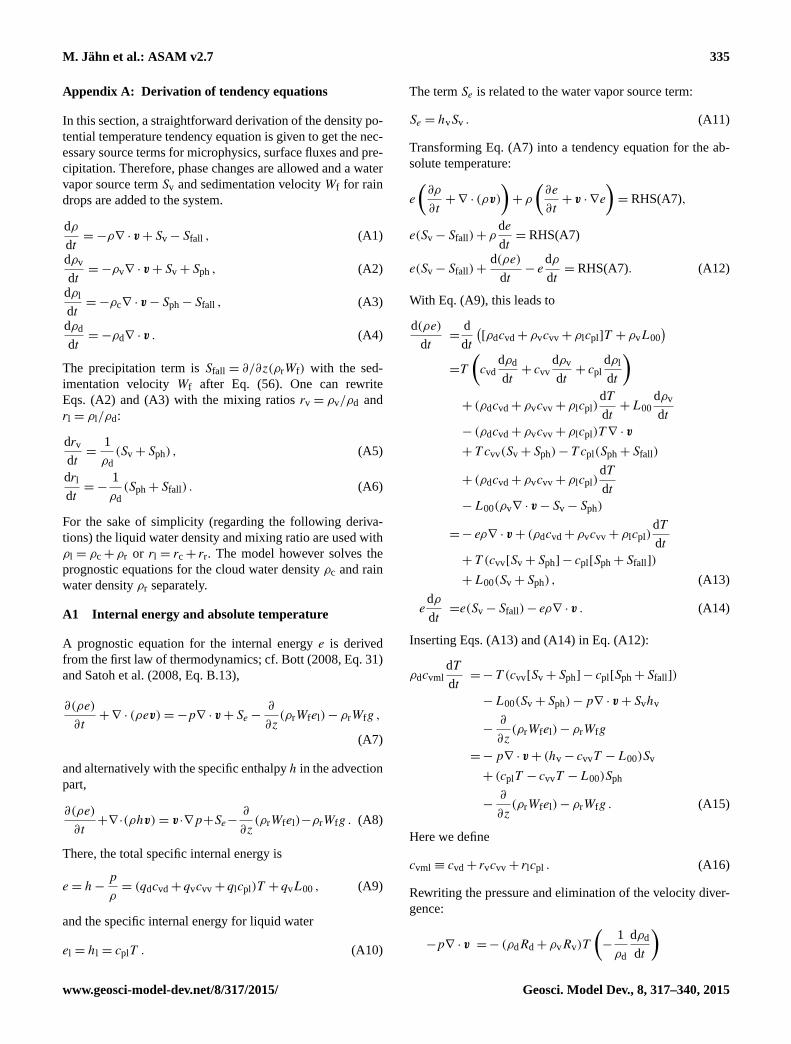
M. Jähn et al.: ASAM v2.7 335
Appendix A: Derivation of tendency equations
In this section, a straightforward derivation of the density po-
tential temperature tendency equation is given to get the nec-
essary source terms for microphysics, surface fluxes and pre-
cipitation. Therefore, phase changes are allowed and a water
vapor source term Sv and sedimentation velocity Wf for rain
drops are added to the system.
dρ
dt=−ρ∇ · v+ Sv− Sfall , (A1)
dρv
dt=−ρv∇ · v+ Sv+ Sph , (A2)
dρl
dt=−ρc∇ · v− Sph− Sfall , (A3)
dρd
dt=−ρd∇ · v . (A4)
The precipitation term is Sfall = ∂/∂z(ρrWf) with the sed-
imentation velocity Wf after Eq. (56). One can rewrite
Eqs. (A2) and (A3) with the mixing ratios rv = ρv/ρd and
rl = ρl/ρd:
drv
dt=
1
ρd
(Sv+ Sph) , (A5)
drl
dt=−
1
ρd
(Sph+ Sfall) . (A6)
For the sake of simplicity (regarding the following deriva-
tions) the liquid water density and mixing ratio are used with
ρl = ρc+ ρr or rl = rc+ rr. The model however solves the
prognostic equations for the cloud water density ρc and rain
water density ρr separately.
A1 Internal energy and absolute temperature
A prognostic equation for the internal energy e is derived
from the first law of thermodynamics; cf. Bott (2008, Eq. 31)
and Satoh et al. (2008, Eq. B.13),
∂(ρe)
∂t+∇ · (ρev)=−p∇ · v+ Se−
∂
∂z(ρrWfel)− ρrWfg ,
(A7)
and alternatively with the specific enthalpy h in the advection
part,
∂(ρe)
∂t+∇·(ρhv)= v ·∇p+Se−
∂
∂z(ρrWfel)−ρrWfg . (A8)
There, the total specific internal energy is
e = h−p
ρ= (qdcvd+ qvcvv+ qlcpl)T + qvL00 , (A9)
and the specific internal energy for liquid water
el = hl = cplT . (A10)
The term Se is related to the water vapor source term:
Se = hvSv . (A11)
Transforming Eq. (A7) into a tendency equation for the ab-
solute temperature:
e
(∂ρ
∂t+∇ · (ρv)
)+ ρ
(∂e
∂t+ v · ∇e
)= RHS(A7),
e(Sv− Sfall)+ ρde
dt= RHS(A7)
e(Sv− Sfall)+d(ρe)
dt− e
dρ
dt= RHS(A7). (A12)
With Eq. (A9), this leads to
d(ρe)
dt=
d
dt
([ρdcvd+ ρvcvv+ ρlcpl]T + ρvL00
)=T
(cvd
dρd
dt+ cvv
dρv
dt+ cpl
dρl
dt
)+ (ρdcvd+ ρvcvv+ ρlcpl)
dT
dt+L00
dρv
dt
− (ρdcvd+ ρvcvv+ ρlcpl)T∇ · v
+ T cvv(Sv+ Sph)− T cpl(Sph+ Sfall)
+ (ρdcvd+ ρvcvv+ ρlcpl)dT
dt
−L00(ρv∇ · v− Sv− Sph)
=− eρ∇ · v+ (ρdcvd+ ρvcvv+ ρlcpl)dT
dt
+ T (cvv[Sv+ Sph] − cpl[Sph+ Sfall])
+L00(Sv+ Sph) , (A13)
edρ
dt=e(Sv− Sfall)− eρ∇ · v . (A14)
Inserting Eqs. (A13) and (A14) in Eq. (A12):
ρdcvml
dT
dt=− T (cvv[Sv+ Sph] − cpl[Sph+ Sfall])
−L00(Sv+ Sph)−p∇ · v+ Svhv
−∂
∂z(ρrWfel)− ρrWfg
=−p∇ · v+ (hv− cvvT −L00)Sv
+ (cplT − cvvT −L00)Sph
−∂
∂z(ρrWfel)− ρrWfg . (A15)
Here we define
cvml ≡ cvd+ rvcvv+ rlcpl . (A16)
Rewriting the pressure and elimination of the velocity diver-
gence:
−p∇ · v =− (ρdRd+ ρvRv)T
(−
1
ρd
dρd
dt
)
www.geosci-model-dev.net/8/317/2015/ Geosci. Model Dev., 8, 317–340, 2015
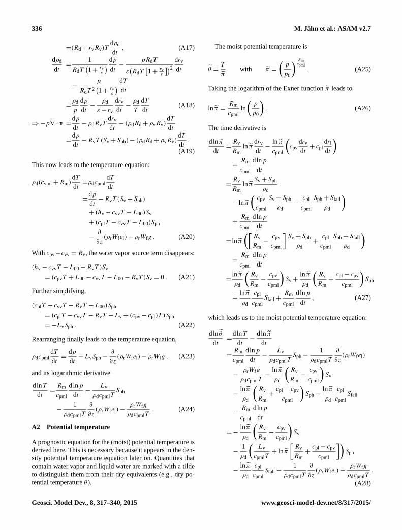
336 M. Jähn et al.: ASAM v2.7
=(Rd+ rvRv)Tdρd
dt, (A17)
dρd
dt=
1
RdT(1+ rv
ε
) dp
dt−
pRdT
ε(RdT
[1+ rv
ε
])2 drv
dt
−p
RdT 2(1+ rv
ε
) dT
dt
=ρd
p
dp
dt−
ρd
ε+ rv
drv
dt−ρd
T
dT
dt(A18)
⇒−p∇ · v =dp
dt− ρdRvT
drv
dt− (ρdRd+ ρvRv)
dT
dt
=dp
dt−RvT (Sv+ Sph)− (ρdRd+ ρvRv)
dT
dt.
(A19)
This now leads to the temperature equation:
ρd(cvml+Rm)dT
dt=ρdcpml
dT
dt
=dp
dt−RvT (Sv+ Sph)
+ (hv− cvvT −L00)Sv
+ (cplT − cvvT −L00)Sph
−∂
∂z(ρrWfel)− ρrWfg . (A20)
With cpv−cvv = Rv, the water vapor source term disappears:
(hv− cvvT −L00−RvT )Sv
= (cpvT +L00− cvvT −L00−RvT )Sv = 0 . (A21)
Further simplifying,
(cplT − cvvT −RvT −L00)Sph
= (cplT − cvvT −RvT −Lv+ (cpv− cpl)T )Sph
=−LvSph . (A22)
Rearranging finally leads to the temperature equation,
ρdcpml
dT
dt=
dp
dt−LvSph−
∂
∂z(ρrWfel)− ρrWfg , (A23)
and its logarithmic derivative
dlnT
dt=Rm
cpml
dlnp
dt−
Lv
ρdcpmlTSph
−1
ρdcpmlT
∂
∂z(ρrWfel)−
ρrWfg
ρdcpmlT. (A24)
A2 Potential temperature
A prognostic equation for the (moist) potential temperature is
derived here. This is necessary because it appears in the den-
sity potential temperature equation later on. Quantities that
contain water vapor and liquid water are marked with a tilde
to distinguish them from their dry equivalents (e.g., dry po-
tential temperature θ ).
The moist potential temperature is
θ =T
πwith π =
(p
p0
) Rmcpml
. (A25)
Taking the logarithm of the Exner function π leads to
ln π =Rm
cpml
ln
(p
p0
). (A26)
The time derivative is
d ln π
dt=Rv
Rm
ln πdrv
dt−
ln π
cpml
(cpv
drv
dt+ cpl
drl
dt
)+Rm
cpml
dlnp
dt
=Rv
Rm
ln πSv+ Sph
ρd
− ln π
(cpv
cpml
Sv+ Sph
ρd
−cpl
cpml
Sph+ Sfall
ρd
)+Rm
cpml
dlnp
dt
= ln π
([Rv
Rm
−cpv
cpml
]Sv+ Sph
ρd
+cpl
cpml
Sph+ Sfall
ρd
)+Rm
cpml
dlnp
dt
=ln π
ρd
(Rv
Rm
−cpv
cpml
)Sv+
ln π
ρd
(Rv
Rm
+cpl− cpv
cpml
)Sph
+ln π
ρd
cpl
cpml
Sfall+Rm
cpml
dlnp
dt, (A27)
which leads us to the moist potential temperature equation:
d ln θ
dt=
dlnT
dt−
dln π
dt
=Rm
cpml
dlnp
dt−
Lv
ρdcpmlTSph−
1
ρdcpmlT
∂
∂z(ρrWfel)
−ρrWfg
ρdcpmlT−
ln π
ρd
(Rv
Rm
−cpv
cpml
)Sv
−ln π
ρd
(Rv
Rm
+cpl− cpv
cpml
)Sph−
ln π
ρd
cpl
cpml
Sfall
−Rm
cpml
dlnp
dt
=−ln π
ρd
(Rv
Rm
−cpv
cpml
)Sv
−1
ρd
(Lv
cpmlT+ ln π
[Rv
Rm
+cpl− cpv
cpml
])Sph
−ln π
ρd
cpl
cpml
Sfall−1
ρdcpmlT
∂
∂z(ρrWfel)−
ρrWfg
ρdcpmlT.
(A28)
Geosci. Model Dev., 8, 317–340, 2015 www.geosci-model-dev.net/8/317/2015/
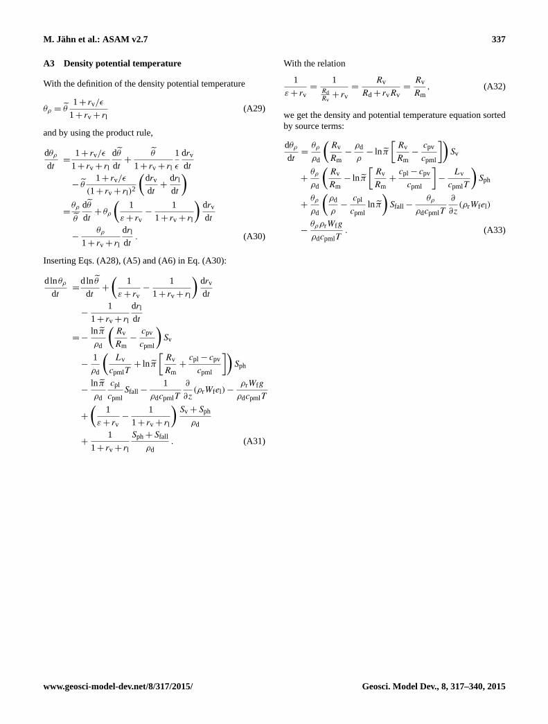
M. Jähn et al.: ASAM v2.7 337
A3 Density potential temperature
With the definition of the density potential temperature
θρ = θ1+ rv/ε
1+ rv+ rl(A29)
and by using the product rule,
dθρ
dt=
1+ rv/ε
1+ rv+ rl
dθ
dt+
θ
1+ rv+ rl
1
ε
drv
dt
− θ1+ rv/ε
(1+ rv+ rl)2
(drv
dt+
drl
dt
)=θρ
θ
dθ
dt+ θρ
(1
ε+ rv−
1
1+ rv+ rl
)drv
dt
−θρ
1+ rv+ rl
drl
dt. (A30)
Inserting Eqs. (A28), (A5) and (A6) in Eq. (A30):
d lnθρ
dt=
dln θ
dt+
(1
ε+ rv−
1
1+ rv+ rl
)drv
dt
−1
1+ rv+ rl
drl
dt
=−ln π
ρd
(Rv
Rm
−cpv
cpml
)Sv
−1
ρd
(Lv
cpmlT+ ln π
[Rv
Rm
+cpl− cpv
cpml
])Sph
−ln π
ρd
cpl
cpml
Sfall−1
ρdcpmlT
∂
∂z(ρrWfel)−
ρrWfg
ρdcpmlT
+
(1
ε+ rv−
1
1+ rv+ rl
)Sv+ Sph
ρd
+1
1+ rv+ rl
Sph+ Sfall
ρd
. (A31)
With the relation
1
ε+ rv=
1
Rd
Rv+ rv=
Rv
Rd+ rvRv
=Rv
Rm
, (A32)
we get the density and potential temperature equation sorted
by source terms:
dθρ
dt=θρ
ρd
(Rv
Rm
−ρd
ρ− ln π
[Rv
Rm
−cpv
cpml
])Sv
+θρ
ρd
(Rv
Rm
− ln π
[Rv
Rm
+cpl− cpv
cpml
]−
Lv
cpmlT
)Sph
+θρ
ρd
(ρd
ρ−cpl
cpml
ln π
)Sfall−
θρ
ρdcpmlT
∂
∂z(ρrWfel)
−θρρrWfg
ρdcpmlT. (A33)
www.geosci-model-dev.net/8/317/2015/ Geosci. Model Dev., 8, 317–340, 2015
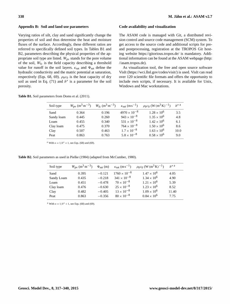
338 M. Jähn et al.: ASAM v2.7
Appendix B: Soil and land use parameters
Varying ratios of silt, clay and sand significantly change the
properties of soil and thus determine the heat and moisture
fluxes of the surface. Accordingly, these different ratios are
referred to specifically defined soil types. In Tables B1 and
B2, parameters describing the physical properties of the ap-
propriate soil type are listed. Wpv stands for the pore volume
of the soil, Wfc is the field capacity describing a threshold
value for runoff in the soil layers. κsat and 9sat define the
hydraulic conductivity and the matric potential at saturation,
respectively (Eqs. 68, 69). ρ0c0 is the heat capacity of dry
soil as used in Eq. (71) and b∗ is a parameter for the soil
porosity.
Table B1. Soil parameters from Doms et al. (2011).
Soil type Wpv (m3 m−3) Wfc (m3 m−3) κsat (ms−1) ρ0c0 (W (m3 K)−1) b∗ a
Sand 0.364 0.196 4970× 10−8 1.28× 10⁶ 3.5
Sandy loam 0.445 0.260 943× 10−8 1.35× 10⁶ 4.8
Loam 0.455 0.340 531× 10−8 1.42× 10⁶ 6.1
Clay loam 0.475 0.370 764× 10−8 1.50× 10⁶ 8.6
Clay 0.507 0.463 1.7× 10⁻⁸ 1.63× 10⁶ 10.0
Peat 0.863 0.763 5.8× 10⁻⁸ 0.58× 10⁶ 9.0
a With n= 1/b∗ + 1, see Eqs. (68) and (69).
Table B2. Soil parameters as used in Pielke (1984) (adapted from McCumber, 1980).
Soil type Wpv (m3 m−3) 9sat (m) κsat (ms−1) ρ0c0 (W (m3 K)−1) b∗ a
Sand 0.395 −0.121 1760× 10−8 1.47× 10⁶ 4.05
Sandy Loam 0.435 −0.218 341× 10−8 1.34× 10⁶ 4.90
Loam 0.451 −0.478 70× 10−8 1.21× 10⁶ 5.39
Clay loam 0.476 −0.630 25× 10−8 1.23× 10⁶ 8.52
Clay 0.482 −0.405 13× 10−8 1.09× 10⁶ 11.40
Peat 0.863 −0.356 80× 10−8 0.84× 10⁶ 7.75
a With n= 1/b∗ + 1, see Eqs. (68) and (69).
Code availability and visualization
The ASAM code is managed with Git, a distributed revi-
sion control and source code management (SCM) system. To
get access to the source code and additional scripts for pre-
and postprocessing, registration at the TROPOS Git host-
ing website https://gitorious.tropos.de/ is mandatory. Addi-
tional information can be found at the ASAM webpage (http:
//asam.tropos.de).
As visualization tool, the free and open source software
VisIt (https://wci.llnl.gov/codes/visit/) is used. VisIt can read
over 120 scientific file formats and offers the opportunity to
include own scripts, if necessary. It is available for Unix,
Windows and Mac workstations.
Geosci. Model Dev., 8, 317–340, 2015 www.geosci-model-dev.net/8/317/2015/
M. Jähn et al.: ASAM v2.7 339
Acknowledgements. This work is internally funded by TROPOS.
The authors like to thank Luca Bonaventura and the anonymous
reviewer for their constructive comments to improve the quality
of the paper. We are also grateful to our technical employees
Sabine Reutgen and Birgit Heinrich for developing and maintaining
the grid generator as well as data maintenance and converting,
respectively.
Edited by: H. Weller
References
Adcroft, A., Hill, C., and Marshall, J.: Representation of topogra-
phy by shaved cells in a height coordinate ocean model, Mon.
Weather Rev., 125, 2293–2315, 1997.
Berger, M. and Helzel, C.: A Simplified h-Box Method for Embed-
ded Boundary Grids, Siam J. Sci. Comput., 34, A861–A888.
Bott, A.: Theoretical considerations on the mass and energy con-
sistent treatment of precipitation in cloudy atmospheres, Atmos.
Res., 89, 262–269, 2008.
Braun, F. J.: Mesoskalige Modellierung der Bodenhydrologie, Wiss.
Berichte des Inst. f. Meteor. u. Klimat. d. Universität Karlsruhe,
30, 2002.
Bryan, G. H. and Fritsch, J. M.: A benchmark simulation for
moist nonhydrostatic numerical models, Mon. Weather Rev.,
130, 2917–2928, 2002.
Chen, F. and Dudhia, J.: Coupling an advanced land surface–
hydrology model with the Penn State-NCAR MM5 modeling
system. Part I: Model implementation and sensitivity, Mon.
Weather Rev., 129, 569–585, 2001.
Cheng, Y. and Brutsaert, W.: Flux-profile relationships for wind
speed and temperature in the stable atmospheric boundary layer,
Bound.-Lay. Meteorol., 114, 519–53, 2005.
Deardorff, J. W.: Numerical investigation of neutral und unstable
boundary layers, J. Atmos. Sci., 29, 91–115, 1972.
Doms, G., Förstner, J., Heise, E., Herzog, H.-J., Mironov, D.,
Raschendorfer, M., Reinhardt, T., Ritter, B., Schrodin, R.,
Schulz, J.-P., and Vogel, G.: A Description of the Nonhydrostatic
Regional COSMO Model, Deutscher Wetterdienst, 2011.
Dongarra, J. J., Duff, I. S., Sorensen, D. C., and van der Vorst, H. A.:
Numerical Linear Algebra for High-Performance Computers,
Society for Industrial and Applied Mathematics, 1998.
Doyle, J. D., Gaberšek, S., Jiang, Q., Bernardet, L., Brown, J. M.,
Dörnbrack, A., Filaus, E., Grubišic, V., Knoth, O., Koch, S.,
Schmidli, J., Stiperski, I., Vosper, S. and Zhong, S.: An Inter-
comparison of T-REX Mountain-Wave Simulations and Impli-
cations for Mesoscale Predictability, Mon. Weather Rev., 139,
2811–2831, 2011.
Eisenstat, S.: Efficient implementation of a class of CG methods,
SIAM J. Sci. Stat. Comput., 2, 1–4, 1981.
Emanuel, K. A.: Atmospheric Convection, Oxford University Press,
1994.
Engelmann, R., Ansmann, A., Horn, S., Seifert, P., Althausen, D.,
Tesche, M., Esselborn, M., Fruntke, J., Lieke, K., Freuden-
thaler, V., and Gross, S.: Doppler lidar studies of heat island ef-
fects on vertical mixing of aerosols during SAMUM-2, Tellus B,
63, 448–458, 2011.
Fairall, C. W., Bradley, E. F., Rogers, D. P., Edson, J. B., and
Young, G. S.: Bulk parameterization of air-sea fluxes for Tropi-
cal Ocean Global Atmosphere Coupled-Ocean Atmosphere Re-
sponse Experiment, J. Geophys. Res., 101, 3747–3764, 1996.
Good, B., Gadian, A., Lock, S. J., and Ross, A.: Performance of the
cut-cell method of representing orography in idealized simula-
tions, Atmos. Sci. Lett., 15, 44–49, 2014.
Hairer, E. and Wanner, G.: Solving Ordinary Differential Equations
II, Springer, 1996.
Hicken, J., Ham, F., Militzer, J., and Koksal, M.: A shift transfor-
mation for fully conservative methods: turbulence simulation on
complex, unstructured grids, J. Comput. Phys., 208, 704–714,
2005.
Hinneburg, D. and Knoth, O.: Non-dissipative cloud transport in
Eulerian grid models by the volume-of-fluid (VOF) method, At-
mos. Environ., 39, 4321–4330, 2005.
Horn, S.: ASAMgpu V1.0 – a moist fully compressible atmospheric
model using graphics processing units (GPUs), Geosci. Model
Dev., 5, 345–353, doi:10.5194/gmd-5-345-2012, 2012.
Hundsdorfer, W., Koren, B., Loon, M. V., and Verwer, J. G.: A pos-
itive finite-difference advection scheme, J. Comput. Phys., 117,
35–46, 1995.
Jebens, S., Knoth, O., and Weiner, R.: Partially implicit peer meth-
ods for the compressible Euler equations, J. Comput. Phys., 230,
4955–4974, 2011.
Jiménez, P. A., Dudhia, J., González-Rouco, J. F., Navarro, J., Mon-
távez, J. P., and García-Bustamante, E.: A revised scheme for the
WRF surface layer formulation, Mon. Weather Rev., 140, 898–
918, 2012.
John, V. and Rang, J.: Adaptive time step control for the in-
compressible Navier-Stokes equations, Comput. Methods Appl.
Mech. Engrg., 199, 514–524, 2010.
Klein, R., Bates, K. R., and Nikiforakis, N.,: Well Balanced Com-
pressible Cut-Cell Simulation of Atmospheric Flow, Phil. Trans.
R. Soc. B, 367, 4559–4575, 2009.
Kleissl, J., Kumar, V., Meneveau, C., and Parlange, M. B.: Nu-
merical study of dynamic Smagorinsky models in large-eddy
simulation of the atmospheric boundary layer: validation in sta-
ble and unstable conditions, Water Resour. Res., 42, W06D10,
doi:10.1029/2005WR004685, 2006.
König, M.: Large-eddy simulation modelling for urban Scale, Ph.D.
thesis, University of Leipzig, 2013.
Knoth, O.: Compressible atmospheric modeling at all scales, in:
Oberwolfach Reports 3, Workshop: Mathematical Theory and
Modelling in Atmosphere-Ocean Science, 2374–2377, 2006.
Kong, L. C., Tunçel, L., and Xiu, N. H.: The Fischer–Burmeister
complementarity function on Euclidean Jordan algebras, Pac. J.
Optim., 6, 423–440, 2010.
Kunz, M. and Wassermann, S.: Sensitivity of flow dynam-
ics and orographic precipitation to changing ambient condi-
tions in idealised model simulations, Meteor. Z., 20, 199–215,
doi:10.1127/0941-2948/2011/0221, 2011.
Lanser, D., Blom, J. G., and Verwer, J. G.: Time integration of the
shallow water equations in spherical geometry, J. Comput. Phys.,
171, 373–393, 2001.
Lilly, D. K.: On the numerical simulation of buoyant convection,
Tellus, 14, 148–172, 1962.
www.geosci-model-dev.net/8/317/2015/ Geosci. Model Dev., 8, 317–340, 2015
340 M. Jähn et al.: ASAM v2.7
Lilly, D. K.: The representation of small scale turbulence in numer-
ical simulation experiments, IBM Scientific Computing Sympo-
sium on environmental sciences, 195–210, 1967.
Lock, S.-J., Bitzer, H.-W., Coals, A., Gadian, A., and Mobbs, S.:
Demonstration of a cut-cell representation of 3D orography for
studies of atmospheric flows over very steep hills, Mon. Weather
Rev., 140, 411–424, 2012.
McCumber, M. D.: A numerical simulation of the influence of heat
and moisture fluxes upon mesoscale circulation, Ph.D. thesis,
Dept. of Environmental Science, University of Virginia, Char-
lottesville, VA, 1980.
Ng, Y.-T., Chen, H., Min, C., and Gibou, F.: Guidelines for Poisson
Solvers on Irregular Domains with Dirichlet Boundary Condi-
tions Using the Ghost Fluid Method, J. Sci. Comput., 41, 300–
320, 2009.
Noilhan, J. and Planton, S.: A simple parameterization of land sur-
face processes for meteorological models, Mon. Weather Rev.,
117, 536–549, 1989.
Pielke, R. A.: Mesoscale Meteorological Modeling, 2nd Edn., Aca-
demic Press, 1984.
Porté-Agel, F., Meneveau, C., and Parlange, M. B.: A scale-
dependent dynamic model for large-eddy simulation: application
to a neutral atmospheric boundary layer, J. Fluid Mech., 415,
261–284, 2000.
Satoh, M., Matsuno, T., Tomita, H., Miura, H., Nasuno, T.,
and Iga, S.: Nonhydrostatic icosahedral atmospheric model
(NICAM) for global cloud resolving simulations, J. Comput.
Phys., 227, 3486–3514, 2008.
Skamarock, W. C., Klemp, J. B., Duda, M. G., Fowler, L. D.,
Park, S.-H., and Ringler, T. D.: A multiscale nonhydrostatic at-
mospheric model using centroidal voronoi tesselations and c-grid
staggering, Mon. Weather Rev., 140, 3090–3105, 2012.
Schaer, C., Leuenberger, D., Fuhrer, O., Lüthi, D., and Girard, C.: A
new terrain-following vertical coordinate formulation for atmo-
spheric prediction models, Mon. Weather Rev., 130, 2459–2480,
2002.
Scotti, A., Meneveau, C., and Lilly, D. K.: Generalized Smagorin-
sky model for anisotropic grids, Phys. Fluids A-Fluid, 5, 2306–
2308, 1993.
Seifert, A. and Beheng, K. D.: A two-moment cloud micro-
physics parameterization for mixed-phase clouds, Meteorol. At-
mos. Phys., 92, 45–66, 2006.
Skamarock, W. C., Klemp, J. B., Dudhia, J., Gill, D. O., Barker, M.,
Duda, K. G., Huang, X. Y., Wang, W., and Powers, J. G.: A de-
scription of the Advanced Research WRF Version 3, Tech. rep.,
National Center for Atmospheric Research, 2008.
Smagorinsky, J.: General circulation experiments with the primitive
equations, Mon. Weather Rev., 164, 91–99, 1963.
Steppeler, J., Bitzer, H.-W., Minotte, M., and Bonaventura, L.: Non-
hydrostatic atmospheric modeling using a z-coordinate represen-
tation, Mon. Weather Rev., 130, 2143–2149, 2002.
Steppeler, J., Bitzer, H.-W., Janjic, Z., Schättler, U., Prohl, P., Gjert-
sen, U., Torrisi, L., Parfinievicz, J., Avgoustoglou, E ., and Dam-
rath, U.: Prediction of Clouds and Rain Using a z-Coordinate
Nonhydrostatic Model, Mon. Weather Rev., 134, 3625–3643,
2006.
Steppeler, J., Park, S.-H. and Dobler, A.: Forecasts covering one
month using a cut-cell model, Geosci. Model Dev., 6, 875–882,
2013.
Straka, J. M., Wilhelmson, R. B., Wicker, L. J., Anderson, J. R., and
Droegemeier, K. K.: Numerical solutions of a non-linear density
current: a benchmark solution and comparisons, Int. J. Numer.
Meth. Fl., 17, 1–22, 1993.
Sweby, P. K.: High resolution schemes using flux limiters for hyper-
bolic conservation laws, SIAM J. Numer. Anal., 21, 995–1011,
1984.
Tripoli, G. J. and Smith, E. A.: Introducing Variable-Step Topog-
raphy (VST) coordinates within dynamically constrained Non-
hydrostatic Modeling System (NMS). Part 1: VST formulation
within NMS host model framework, Dynam. Atmos. Oceans, 66,
28–57, 2014a.
Tripoli, G. J. and Smith, E. A.: Introducing Variable-Step Topog-
raphy (VST) coordinates within dynamically constrained Non-
hydrostatic Modeling System (NMS). Part 2: VST performance
on orthodox obstacle flows, Dynam. Atmos. Oceans, 66, 10–27,
2014b.
Van Genuchten, M. T.: A closed-form equation for predicting the
hydraulic conductivity of unsaturated soils, Soil Sci. Soc. Am.
J., 44, 892–898, 1980.
Van Leer, B.: Upwind-difference methods for aerodynamic prob-
lems governed by the Euler equations, in: Lectures in Applied
Mathematics, 327–336, 1994.
Walko, R. L. and Avissar, R.: The Ocean–Land–Atmosphere Model
(OLAM). Part I: Shallow-water tests, Mon. Weather Rev., 136,
4033–4044, 2008a.
Walko, R. L. and Avissar, R.: The Ocean–Land–Atmosphere Model
(OLAM). Part II: Formulation and tests of the nonhydrostatic dy-
namic core, Mon. Weather Rev., 136, 4045–4062, 2008b.
Wicker, L. J. and Skamarock, W. C.: A time-splitting scheme for the
elastic equations incorporating second-order Runge–Kutta time
differencing, Mon. Weather Rev., 126, 1992–1999, 1998.
Yamazaki, H. and Satomura, T.: Vertically combined shaved cell
method in a z-coordinate nonhydrostatic atmospheric model, At-
mos. Sci. Lett., 9, 171–175, 2008.
Yamazaki, H. and Satomura, T.: Nonhydrostatic Atmospheric Mod-
eling Using a Combined Cartesian Grid, Mon. Weather Rev.,
138, 3932–3945, 2010.
Yamazaki, H. and Satomura, T.: Non-hydrostatic atmospheric cut
cell model on a block-structured mesh, Atmos. Sci. Lett., 13, 29–
35, 2012.
Geosci. Model Dev., 8, 317–340, 2015 www.geosci-model-dev.net/8/317/2015/


