Reconstruction of Undersampled Non-Cartesian Data SetsUsing Pseudo-Cartesian GRAPPA in Conjunction WithGROG

Nicole Seiberlich,1* Felix Breuer,2 Robin Heidemann,3 Martin Blaimer,2

Mark Griswold,4 and Peter Jakob1,2

Most k-space-based parallel imaging reconstruction tech-niques, such as Generalized Autocalibrating Partially ParallelAcquisitions (GRAPPA), necessitate the acquisition of regularlysampled Cartesian k-space data to reconstruct a nonaliasedimage efficiently. However, non-Cartesian sampling schemesoffer some inherent advantages to the user due to their bettercoverage of the center of k-space and faster acquisition times.On the other hand, these sampling schemes have the disadvan-tage that the points acquired generally do not lie on a grid andhave complex k-space sampling patterns. Thus, the extensionof Cartesian GRAPPA to non-Cartesian sequences is nontrivial.This study introduces a simple, novel method for performingCartesian GRAPPA reconstructions on undersampled non-Car-tesian k-space data gridded using GROG (GRAPPA OperatorGridding) to arrive at a nonaliased image. Because the under-sampled non-Cartesian data cannot be reconstructed using asingle GRAPPA kernel, several Cartesian patterns are selectedfor the reconstruction. This flexibility in terms of both the ap-pearance and number of patterns allows this pseudo-CartesianGRAPPA to be used with undersampled data sets acquired withany non-Cartesian trajectory. The successful implementation ofthe reconstruction algorithm using several different trajecto-ries, including radial, rosette, spiral, one-dimensional non-Car-tesian, and zig–zag trajectories, is demonstrated. Magn Re-son Med 59:1127–1137, 2008. © 2008 Wiley-Liss, Inc.

Key words: parallel imaging; non-Cartesian trajectories;GRAPPA; GROG

One of the most important factors to be considered in animaging sequence is the total acquisition time. Time-re-duction methods such as parallel imaging (1–8) and alter-native k-space sampling schemes, such as spiral (9,10) orradial (11,12) acquisitions, have been separately investi-gated, and both have been shown to decrease the amountof time needed to acquire an image. Parallel imaging usesthe differing spatial sensitivity information of multi-coilreceiver arrays to partially replace some information typ-ically gathered using gradient encoding. The missing data

are then reconstructed using one of several techniques,such as SMASH (1), SENSE (3), or GRAPPA (8), designedto use coil sensitivities to obtain spatial information,which can be used in place of phase encoding.

Non-Cartesian k-space trajectories, on the other hand,can reduce scan time by minimizing the number of exci-tations needed to cover k-space. In addition to faster scantimes, different trajectories have added advantages, suchas the motion-insensitivity of radial trajectories, the abilityto perform motion correction using the PROPELLER tra-jectory (13,14), or the possibility of obtaining spectral in-formation using the rosette trajectory (15). These proper-ties make such sampling schemes highly desirable, and thecombination of non-Cartesian trajectories and parallel im-aging would be ideal in cases where a further reduction inscan time is advantageous.

Unfortunately, the combination of these parallel imag-ing techniques and non-Cartesian sampling is not trivial,as the aliasing which results from undersampled non-Cartesian data is more complex than the Cartesian casedue to the unusual point spread functions (16,17). Pruess-mann et al. have demonstrated a method for the recon-struction of undersampled non-Cartesian trajectories usingthe SENSE algorithm in combination with a conjugate-gradient iteration approach (18). Other authors haveshown that the combination of other parallel imagingmethods and non-Cartesian trajectories is possible, al-though time-consuming due to the large system of linearequations that must be solved (19–21). Similarly, severalauthors have shown that the combination of GRAPPA andradial (22) and spiral (23,24) trajectories can be performedmore efficiently, although these techniques require radialsegmentation of the data before the application of thereconstruction algorithm and large amounts of autocalibra-tion data (ACS). One-dimensional (1D) non-Cartesian (25)and zig–zag (26) trajectories can also be combined withGRAPPA, although they require weight interpolation andsegmentation respectively, due to the lack of Cartesiansymmetry. These difficulties arise because the standardGRAPPA reconstruction procedure requires regular,evenly spaced undersampled data, which is not generallythe case in non-Cartesian data. However, some trajectories,such as rosette (15) or TwiRL (27), do not possess thesymmetry required for the segmentation approach; thissuggests that neither Cartesian nor non-Cartesian GRAPPAtechniques are able to reconstruct images from under-sampled data along these trajectories.

In contrast, the method proposed here does not rely onthe radial symmetry of non-Cartesian trajectories, but in-stead uses several Cartesian GRAPPA patterns to recon-

1Department of Experimental Physics 5, University of Wurzburg, Germany.2Research Center Magnetic Resonance Bavaria (MRB), Wurzburg, Germany.3Max Planck Institute for Human Cognitive and Brain Science, Leipzig, Ger-many.4Department of Radiology, University Hospitals of Cleveland, Cleveland, Ohio.Grant sponsor: the German Research Society (Deutsche Forschungsgemein-schaft, DFG); Grant number: JA 827/1-4; Grant sponsor: Siemens MedicalSolutions.*Correspondence to: Nicole Seiberlich, Physikalisches Institut, EP 5, Univer-sitat Wurzburg, Am Hubland, D-97074 Wurzburg, Germany. E-mail:neseiber@physik.uni-wuerzburg.deReceived 28 June 2007; revised 28 January 2008; accepted 30 January 2008.DOI 10.1002/mrm.21602Published online in Wiley InterScience (www.interscience.wiley.com).

Magnetic Resonance in Medicine 59:1127–1137 (2008)

© 2008 Wiley-Liss, Inc. 1127

struct a nonaliased image using gridded undersampleddata sets. The primary advantage of this pseudo-Cartesianmethod over previously proposed non-Cartesian recon-struction schemes is its similarity to the typical CartesianGRAPPA procedure and general applicability to many dif-ferent non-Cartesian sampling schemes. This techniquecan be used to reconstruct an image from an arbitrarynon-Cartesian trajectory, making this reconstructionscheme more general than other non-Cartesian GRAPPAreconstruction techniques.

THEORY

Cartesian and non-Cartesian GRAPPA

Before describing the use of GRAPPA for the reconstruc-tion of non-Cartesian data sets, a simple 2D Cartesian caseshould be examined. In general, an undersampled data setis reconstructed using coil weighting factors derived froma reference data set, or Autocalibration Signal (ACS),which is usually a low-resolution portion of k-space sam-pled at the Nyquist rate. Representative examples of bothfor an acceleration factor R � 4 and a single coil are shownin Figure 1 (the remaining coils, which have the same datastructure, have been omitted from the figure for simplic-ity). An appropriate GRAPPA pattern, in this case, a 2 � 5kernel (where two points in the phase encoding directionand five points in the read direction are selected for thepattern), is shown in the inset of Figure 1. Using thispattern, weighting factors are obtained on a coil-by-coilbasis by examining the relationship between the sourcepoints from all coils and a single target point in the ACS.These weighting factors are subsequently applied to thesource points in the undersampled portion of the data tofind the values of the target points. Because the under-sampled points fall on a regular pattern in the Cartesiandata set, that is, are highly symmetric, only one GRAPPApattern with three target points, and thus one set of coilweighting factors, is needed to reconstruct the missingpoints.

Due to the fact that the GRAPPA technique necessitatesmatching patterns in both the undersampled source dataand the reference data, most common non-CartesianGRAPPA methods make use of the radial symmetry inher-ent in the trajectory. The undersampled radial or spiral

data are first reordered onto a new Cartesian-like grid,where the axes are the read-out (r) and projection angle (�)(22–24). The missing data are then reconstructed using asegmented GRAPPA procedure, which calculates the coilweights for different portions of k-space separately; a sim-ple Cartesian GRAPPA method cannot be used because thedistance and direction between sampled points changesdepending on their location in k-space. Finally, the entirereconstructed Cartesian-like data must be gridded to arriveat the final k-space, upon which a fast Fourier transforma-tion is performed to obtain an image. It is clear that thesemethods necessitate a regular radial symmetry as well asseveral different GRAPPA kernels to reconstruct the miss-ing points in the appropriate locations, and can thus beused only with specific trajectories.

Pseudo-Cartesian GRAPPA

The pseudo-Cartesian GRAPPA method is made up ofthree distinct steps: (1) Gridding the acquired data onto aCartesian grid using GROG; (2) Determination of the ap-propriate pseudo-Cartesian patterns; (3) Reconstruction ofthe missing points using GRAPPA and the selected pat-terns. Each of these three steps is discussed below.

GRAPPA Operator Gridding (GROG)

GROG (28) is a method that uses parallel imaging to gridnon-Cartesian data sets. GROG is a special case ofGRAPPA where the number of source and target points isthe same, usually one. Because of this, the GROG weightsets are square matrices; thus, given the weight set for ajump of 1�k in a single direction, the weight set for asmaller jump, such as 0.5�k, can be found by taking theappropriate root of the weight set for the larger jump:

G1 � G0.52

G0.5 � �G1�0.5

GROG works by using the appropriate root of the baseweight sets to shift each non-Cartesian point to the nearestCartesian location on a grid using the following equationfor a 2D image:

s�kx � �x,ky � �y� � Gx�x � Gy

�y � s�kx,ky�

where s(kx,ky) is a vector containing the non-Cartesiansignal from each of the receiver coils (1 to NC, where NC isthe number of coils) at the k-space location [kx,ky] to beshifted by an amount [�x,�y]; Gx and Gy are the appropriateGROG weight sets of size NC � NC for unit shifts in the xand y directions, respectively; and s(kx��x,ky��y) is theshifted signal at the Cartesian location [kx��x,ky��y]. TheGROG weights Gx and Gy can be determined either fromthe non-Cartesian data themselves (29) or using a separatelow-resolution Cartesian data set and the GRAPPA methodof weight calibration. It is important to note that GROGalone cannot be used to reconstruct undersampled non-Cartesian k-space data because only one source point (non-Cartesian) is used for each target point (Cartesian). The

FIG. 1. A schematic Cartesian R � 4 acquisition scheme. The blackcircles show data that have been acquired, and the empty circlesdata that must be reconstructed using the GRAPPA algorithm and a2 � 5 kernel. The fully sampled central portion of k-space is used asthe Autocalibration Signal (ACS), so it is important that the under-sampled portions maintain the same symmetry. In the smaller figureto the right, the GRAPPA source points (black) are shown, as well asthe points to be reconstructed (gray) using these source points.

1128 Seiberlich et al.

small number of source points suggests that only smallshifts can be accomplished; depending on the coil array,shifts of more than �k � 0.5 in each direction can lead toerrors which result in artifacts in the image domain. Thislimitation does not generally hamper gridding, because thelargest shift required to grid is �k � 0.5, although it meansthat GROG cannot be used alone for the reconstruction ofimages from undersampled non-Cartesian data sets.

GROG is advantageous for gridding because the processcan be performed quickly, as only two weight sets arerequired for the needed k-space shifts, and no densitycompensation function is required. In addition, it has beenshown that GROG can be used to grid fully sampled datasets without a visible increase in the noise in the finalimage when working with clinical coil arrays (28). Specif-ically, symmetric array coils with six or more elements can

be used to perform GROG shifts of �k � 0.5 in both logicaldirections without significant noise enhancement; thus,only such coils were used in this work.

However, in pseudo-Cartesian GRAPPA, GROG is usedfor a different reason. Most other gridding techniques,including the standard convolution gridding method (30),assume that the non-Cartesian data fulfill the Nyquist cri-terion at all locations in k-space. When this is not the case,gridding errors appear. GROG, however, only shifts eachnon-Cartesian data point to its nearest Cartesian neighborusing parallel imaging weight sets. This procedure leavesempty spaces where the shift necessary to reach the nextCartesian data points exceeds the above mentioned valueof �k � 0.5. In comparison, no empty spaces are left in theundersampled k-space data if a conventional gridding ker-nel is used. Due to the convolution of the non-Cartesianpoints with this gridding kernel, a single non-Cartesiandata point is spread out over several Cartesian locations.Thus, pseudo-Cartesian GRAPPA, which requires these“holes” in k-space for the reconstruction, would not bepossible using conventional gridding methods.

Determination of Patterns

Unfortunately, the gridded undersampled data do not con-tain one single Cartesian pattern that is repeated regularlythroughout the data and that can be used with the standardCartesian GRAPPA algorithm, i.e., there is no simple Car-tesian symmetry in the non-Cartesian data set. In spiraldata, for instance, the 2 � 5 GRAPPA kernel forms apattern that would be optimal for a pie-shaped sectorrunning 0° from the center of k-space would be completelyunsuccessful for the sector along the 90° radius (Fig. 2,right), because the selected Cartesian pattern does not existin these data. For this reason, several simple CartesianGRAPPA patterns must be used to cover the entire under-

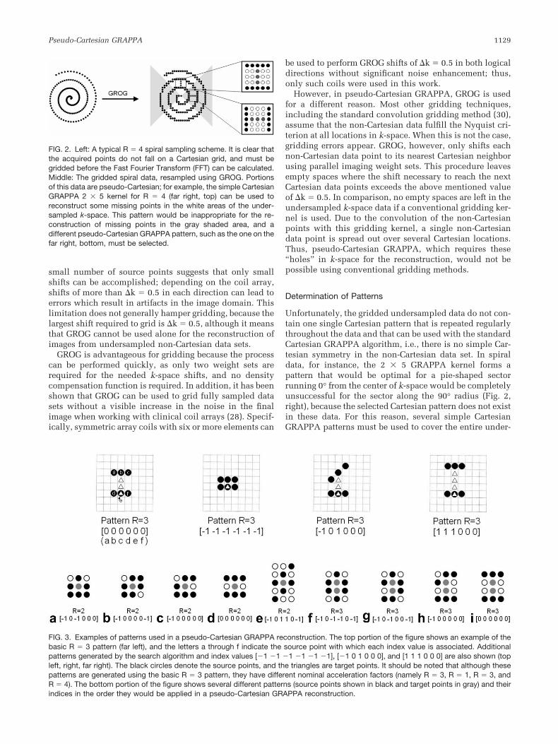
FIG. 2. Left: A typical R � 4 spiral sampling scheme. It is clear thatthe acquired points do not fall on a Cartesian grid, and must begridded before the Fast Fourier Transform (FFT) can be calculated.Middle: The gridded spiral data, resampled using GROG. Portionsof this data are pseudo-Cartesian; for example, the simple CartesianGRAPPA 2 � 5 kernel for R � 4 (far right, top) can be used toreconstruct some missing points in the white areas of the under-sampled k-space. This pattern would be inappropriate for the re-construction of missing points in the gray shaded area, and adifferent pseudo-Cartesian GRAPPA pattern, such as the one on thefar right, bottom, must be selected.

FIG. 3. Examples of patterns used in a pseudo-Cartesian GRAPPA reconstruction. The top portion of the figure shows an example of thebasic R � 3 pattern (far left), and the letters a through f indicate the source point with which each index value is associated. Additionalpatterns generated by the search algorithm and index values [1 1 1 1 1 1], [1 0 1 0 0 0], and [1 1 1 0 0 0] are also shown (topleft, right, far right). The black circles denote the source points, and the triangles are target points. It should be noted that although thesepatterns are generated using the basic R � 3 pattern, they have different nominal acceleration factors (namely R � 3, R � 1, R � 3, andR � 4). The bottom portion of the figure shows several different patterns (source points shown in black and target points in gray) and theirindices in the order they would be applied in a pseudo-Cartesian GRAPPA reconstruction.

Pseudo-Cartesian GRAPPA 1129

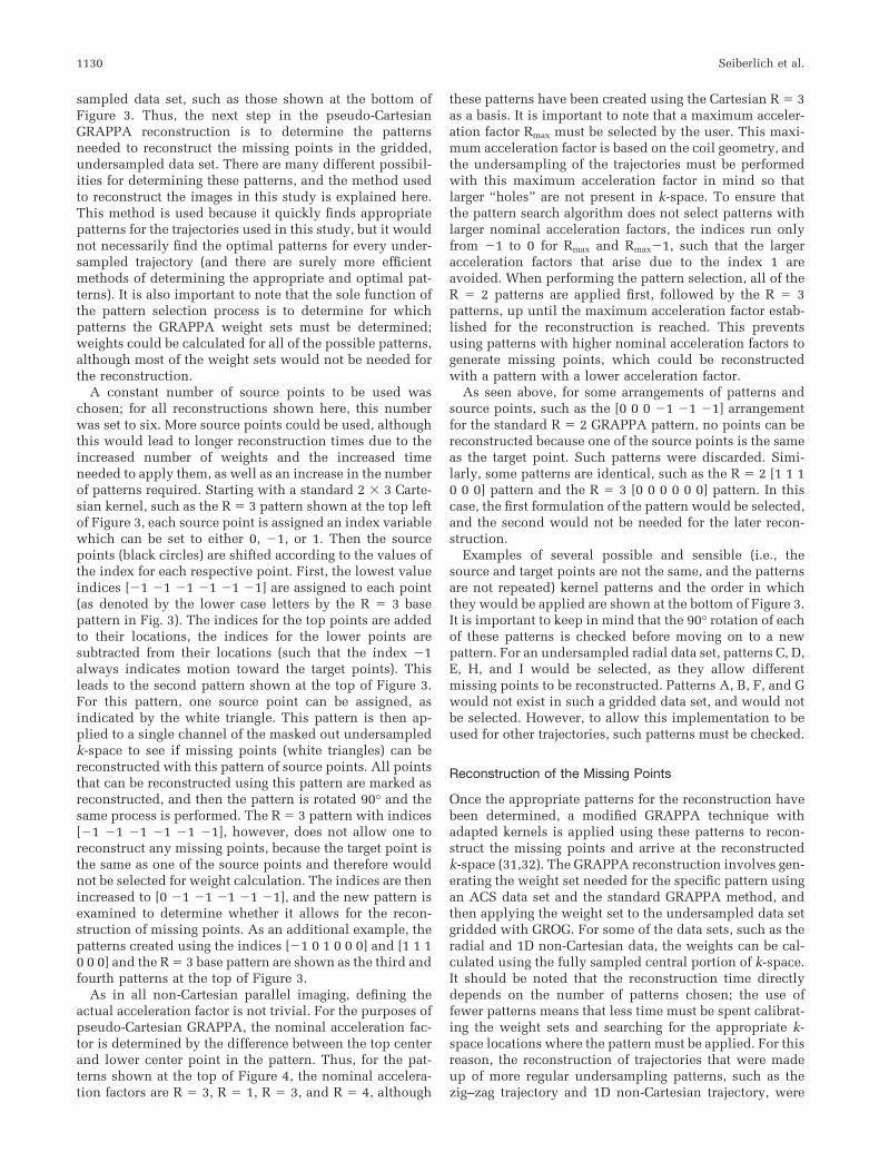
sampled data set, such as those shown at the bottom ofFigure 3. Thus, the next step in the pseudo-CartesianGRAPPA reconstruction is to determine the patternsneeded to reconstruct the missing points in the gridded,undersampled data set. There are many different possibil-ities for determining these patterns, and the method usedto reconstruct the images in this study is explained here.This method is used because it quickly finds appropriatepatterns for the trajectories used in this study, but it wouldnot necessarily find the optimal patterns for every under-sampled trajectory (and there are surely more efficientmethods of determining the appropriate and optimal pat-terns). It is also important to note that the sole function ofthe pattern selection process is to determine for whichpatterns the GRAPPA weight sets must be determined;weights could be calculated for all of the possible patterns,although most of the weight sets would not be needed forthe reconstruction.

A constant number of source points to be used waschosen; for all reconstructions shown here, this numberwas set to six. More source points could be used, althoughthis would lead to longer reconstruction times due to theincreased number of weights and the increased timeneeded to apply them, as well as an increase in the numberof patterns required. Starting with a standard 2 � 3 Carte-sian kernel, such as the R � 3 pattern shown at the top leftof Figure 3, each source point is assigned an index variablewhich can be set to either 0, 1, or 1. Then the sourcepoints (black circles) are shifted according to the values ofthe index for each respective point. First, the lowest valueindices [1 1 1 1 1 1] are assigned to each point(as denoted by the lower case letters by the R � 3 basepattern in Fig. 3). The indices for the top points are addedto their locations, the indices for the lower points aresubtracted from their locations (such that the index 1always indicates motion toward the target points). Thisleads to the second pattern shown at the top of Figure 3.For this pattern, one source point can be assigned, asindicated by the white triangle. This pattern is then ap-plied to a single channel of the masked out undersampledk-space to see if missing points (white triangles) can bereconstructed with this pattern of source points. All pointsthat can be reconstructed using this pattern are marked asreconstructed, and then the pattern is rotated 90° and thesame process is performed. The R � 3 pattern with indices[1 1 1 1 1 1], however, does not allow one toreconstruct any missing points, because the target point isthe same as one of the source points and therefore wouldnot be selected for weight calculation. The indices are thenincreased to [0 1 1 1 1 1], and the new pattern isexamined to determine whether it allows for the recon-struction of missing points. As an additional example, thepatterns created using the indices [1 0 1 0 0 0] and [1 1 10 0 0] and the R � 3 base pattern are shown as the third andfourth patterns at the top of Figure 3.

As in all non-Cartesian parallel imaging, defining theactual acceleration factor is not trivial. For the purposes ofpseudo-Cartesian GRAPPA, the nominal acceleration fac-tor is determined by the difference between the top centerand lower center point in the pattern. Thus, for the pat-terns shown at the top of Figure 4, the nominal accelera-tion factors are R � 3, R � 1, R � 3, and R � 4, although

these patterns have been created using the Cartesian R � 3as a basis. It is important to note that a maximum acceler-ation factor Rmax must be selected by the user. This maxi-mum acceleration factor is based on the coil geometry, andthe undersampling of the trajectories must be performedwith this maximum acceleration factor in mind so thatlarger “holes” are not present in k-space. To ensure thatthe pattern search algorithm does not select patterns withlarger nominal acceleration factors, the indices run onlyfrom 1 to 0 for Rmax and Rmax1, such that the largeracceleration factors that arise due to the index 1 areavoided. When performing the pattern selection, all of theR � 2 patterns are applied first, followed by the R � 3patterns, up until the maximum acceleration factor estab-lished for the reconstruction is reached. This preventsusing patterns with higher nominal acceleration factors togenerate missing points, which could be reconstructedwith a pattern with a lower acceleration factor.

As seen above, for some arrangements of patterns andsource points, such as the [0 0 0 1 1 1] arrangementfor the standard R � 2 GRAPPA pattern, no points can bereconstructed because one of the source points is the sameas the target point. Such patterns were discarded. Simi-larly, some patterns are identical, such as the R � 2 [1 1 10 0 0] pattern and the R � 3 [0 0 0 0 0 0] pattern. In thiscase, the first formulation of the pattern would be selected,and the second would not be needed for the later recon-struction.

Examples of several possible and sensible (i.e., thesource and target points are not the same, and the patternsare not repeated) kernel patterns and the order in whichthey would be applied are shown at the bottom of Figure 3.It is important to keep in mind that the 90° rotation of eachof these patterns is checked before moving on to a newpattern. For an undersampled radial data set, patterns C, D,E, H, and I would be selected, as they allow differentmissing points to be reconstructed. Patterns A, B, F, and Gwould not exist in such a gridded data set, and would notbe selected. However, to allow this implementation to beused for other trajectories, such patterns must be checked.

Reconstruction of the Missing Points

Once the appropriate patterns for the reconstruction havebeen determined, a modified GRAPPA technique withadapted kernels is applied using these patterns to recon-struct the missing points and arrive at the reconstructedk-space (31,32). The GRAPPA reconstruction involves gen-erating the weight set needed for the specific pattern usingan ACS data set and the standard GRAPPA method, andthen applying the weight set to the undersampled data setgridded with GROG. For some of the data sets, such as theradial and 1D non-Cartesian data, the weights can be cal-culated using the fully sampled central portion of k-space.It should be noted that the reconstruction time directlydepends on the number of patterns chosen; the use offewer patterns means that less time must be spent calibrat-ing the weight sets and searching for the appropriate k-space locations where the pattern must be applied. For thisreason, the reconstruction of trajectories that were madeup of more regular undersampling patterns, such as thezig–zag trajectory and 1D non-Cartesian trajectory, were

1130 Seiberlich et al.

much less time consuming than reconstructions using theradial, spiral, or rosette trajectories in this implementa-tion.

METHODS

Data Reconstruction

All fully sampled and undersampled data sets shown inthis manuscript were gridded using GROG. As statedabove, this method has the advantage that single non-Cartesian points are shifted to the nearest Cartesian pointusing the GRAPPA Operator, leaving empty spaces in k-space where data must be reconstructed. For the radial,spiral, and 1D non-Cartesian data sets, the GROG weightswere determined from the data themselves (29); a separatelow-resolution Cartesian k-space was used to calibrate theweights for the rosette and zig–zag trajectories.

After the data were gridded, appropriate patterns foreach undersampled trajectory were determined using thealgorithm described above. To avoid leaving gaps in thereconstructed k-space, a large number of patterns was cho-sen (i.e. between 4 to 102, depending on the trajectory andundersampling factor, see Table 1). Each pattern was ar-ranged in a different configuration with six source points(see Fig. 3 for examples of these patterns).

Once the patterns were determined, the pseudo-Carte-sian GRAPPA reconstruction was performed. First, theweight set for each pattern is found using the ACS in thesame way that the weight sets are derived for GRAPPA,and then this weight set is applied in those places in theundersampled k-space where the specific pattern fits. Forthe radial data set, the ACS was taken from the centralfully sampled portion of the gridded undersampled k-space; for the remaining data sets, the central portion ofthe fully sampled and gridded data was used.

Simulations

To test the feasibility of the method described above, thestandard Shepp-Logan phantom was used with a simu-lated eight-element one-ring head coil array, where sensi-tivities were derived using an analytic integration of theBiot-Savart equations. The Cartesian data were resampledas radial data (50 projections, 256 read-out points, basematrix of 128 � 128) by sinc interpolation, which corre-sponds to an undersampling factor of 4 in comparison tothe fully sampled case. The GROG weights were deter-mined from the radial arms themselves (29), and the un-dersampled radial data were gridded. Using the pattern-finding algorithm described above, it was determined thatthe use of 67 different pseudo-Cartesian GRAPPA patterns

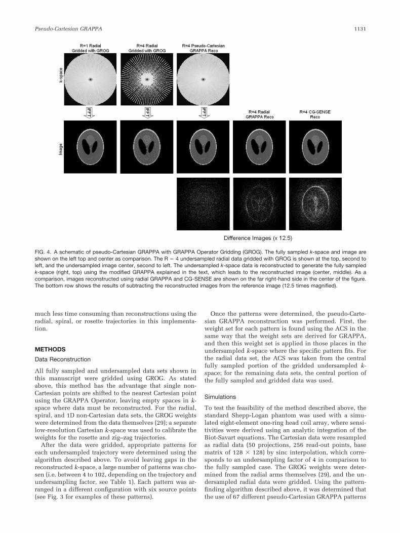
FIG. 4. A schematic of pseudo-Cartesian GRAPPA with GRAPPA Operator Gridding (GROG). The fully sampled k-space and image areshown on the left top and center as comparison. The R � 4 undersampled radial data gridded with GROG is shown at the top, second toleft, and the undersampled image center, second to left. The undersampled k-space data is reconstructed to generate the fully sampledk-space (right, top) using the modified GRAPPA explained in the text, which leads to the reconstructed image (center, middle). As acomparison, images reconstructed using radial GRAPPA and CG-SENSE are shown on the far right-hand side in the center of the figure.The bottom row shows the results of subtracting the reconstructed images from the reference image (12.5 times magnified).

Pseudo-Cartesian GRAPPA 1131

would allow for a complete reconstruction of the missingk-space points given the arrangement of the undersampleddata points. Examples of these patterns are given in Figure3. The reconstruction was then carried out using the 67patterns. As can be seen in Figure 4 (center, top), thecentral portion of k-space is fully sampled, and this block(25 � 25) can be used to determine the weights for thepseudo-Cartesian GRAPPA patterns.

In addition, a standard radial GRAPPA reconstruction(22) with 8 read-out and 10 angular segments was per-formed using the same undersampled radial data set (andthe fully sampled data set as the ACS) to investigate thedifferences in the images between the standard and pro-posed reconstruction techniques. For the standard radialreconstructions shown here, the fully sampled radial k-space data were used for the calibration, although self-calibrating methods have been proposed for radialGRAPPA (33). The use of such a method is not expected tosignificantly change the image quality in this reconstruc-tion. A conjugate-gradient SENSE (CG-SENSE) reconstruc-tion (18) was also performed using 30 iterations of theconjugate gradient loop. Because this method requires acoil sensitivity map, such a map was derived from theradial data set using array correlation statistics (34). TheCG-SENSE algorithm yields a single image instead ofmulti-channel images, and thus the multi-channel images

resulting from the pseudo-Cartesian GRAPPA and radialGRAPPA reconstructions, as well as the reference image,were combined using R � 1 SENSE (3) for comparisonpurposes. After the reconstructions were performed, theresults were subtracted from the reference image to yielddifference images which highlight the reconstruction er-rors.

Finally, an undersampled simulated rosette data set wasgenerated by resampling an in vivo Cartesian head imageusing sinc interpolation to investigate the performance ofpseudo-Cartesian GRAPPA for the rosette trajectory. Thehead coil array used was the same as that used for theradial simulations. The complete data set was made up of120 phase encoding steps, each with 360 read-out points,and the R � 4 accelerated rosette data set was created byreducing the number of phase encoding steps to 30. A totalof 92 patterns were used for the pseudo-CartesianGRAPPA reconstruction, including those shown in Figure4. Both the GROG weights and the weights for the pseudo-Cartesian patterns were derived from a separate low-reso-lution (25 � 25) Cartesian k-space.

In Vivo Experiments

Three images were acquired with two different scanners,namely a Siemens 1.5T Avanto and a Siemens 3T TIM Trio

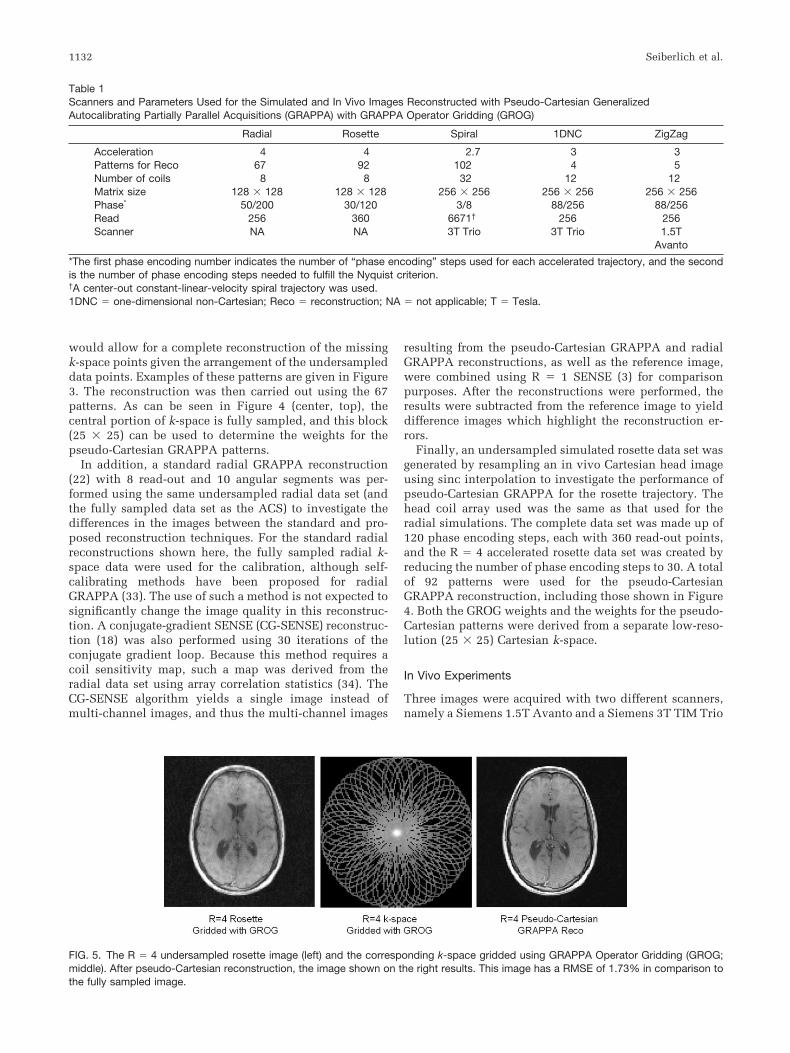
FIG. 5. The R � 4 undersampled rosette image (left) and the corresponding k-space gridded using GRAPPA Operator Gridding (GROG;middle). After pseudo-Cartesian reconstruction, the image shown on the right results. This image has a RMSE of 1.73% in comparison tothe fully sampled image.

Table 1Scanners and Parameters Used for the Simulated and In Vivo Images Reconstructed with Pseudo-Cartesian GeneralizedAutocalibrating Partially Parallel Acquisitions (GRAPPA) with GRAPPA Operator Gridding (GROG)

Radial Rosette Spiral 1DNC ZigZag

Acceleration 4 4 2.7 3 3Patterns for Reco 67 92 102 4 5Number of coils 8 8 32 12 12Matrix size 128 � 128 128 � 128 256 � 256 256 � 256 256 � 256Phase* 50/200 30/120 3/8 88/256 88/256Read 256 360 6671† 256 256Scanner NA NA 3T Trio 3T Trio 1.5T

Avanto

*The first phase encoding number indicates the number of “phase encoding” steps used for each accelerated trajectory, and the secondis the number of phase encoding steps needed to fulfill the Nyquist criterion.†A center-out constant-linear-velocity spiral trajectory was used.1DNC � one-dimensional non-Cartesian; Reco � reconstruction; NA � not applicable; T � Tesla.

1132 Seiberlich et al.

(Siemens Medical Solutions, Erlangen, Germany), to testthe pseudo-Cartesian GRAPPA reconstruction with differ-ent non-Cartesian trajectories, namely spiral, 1D non-Car-tesian, and zig–zag. Informed consent from the volunteerswas obtained before each study. Information about thedata acquisition parameters, scanners, and coils used isshown in Table 1.

The spiral trajectory was used to acquire an image of thebrain accelerated by a factor of 2.7 (3 of 8 spiral armsneeded to fulfill the Nyquist criterion were used). TheGROG weights were calculated using a fully sampled spi-ral data set, and the 102 different pseudo-CartesianGRAPPA weights used were determined using a 30 � 30portion from the center of the fully sampled k-space. Asstated above, each pattern was made up of at least sixsource points; these patterns were similar to those shownin Figure 3 and specifically, patterns D, E, H, and I wereactually used for the reconstruction. In addition to thepseudo-Cartesian GRAPPA reconstruction, a CG-SENSEreconstruction was also performed, where the coil sensi-tivity map was also generated using array correlation sta-tistics [34]. In this CG-SENSE implementation, 50 itera-tions were performed and a grid oversampling factor of 4was used.

An image of a phantom was acquired using the 1Dnon-Cartesian trajectory accelerated by a factor of 3. Thecentral portion of k-space was completely acquired (yield-ing a matrix size of 21 � 256), and was used for thecalibration of both the GROG and the pseudo-Cartesian

weights. Only 4 patterns were required, as the griddedk-space appears purely Cartesian in the x-direction.

Data were also acquired using a version of the R � 3zig–zag trajectory [26] that blipped over approximately 2�ky in 32 cycles of 16 points. Again, the data were griddedusing GROG, where the weights were determined using alow-resolution k-space (40 � 40 vs the original 256 � 256data matrix). Pseudo-Cartesian GRAPPA with 5 patternswas used to reconstruct the missing data points.

RESULTS

Simulations

The k-space and image reconstructed using R � 4 under-sampled radial data and the pseudo-Cartesian GRAPPAmethod are shown in Figure 4 (center right). For compar-ison, the image resulting from the undersampled data set,which displays typical streaking and blurring radial un-dersampling artifacts, is shown in the center of the figure,second from left. The root-mean-square-error (RMSE) ofthe reconstructed image as compared to the fully sampledimage was calculated to be 0.06%, which is similar to thatof the radial GRAPPA image (0.08%, Fig. 3, center, farright), and lower than that of the CG-SENSE image(0.47%). Each reconstruction technique yielded excellentresults, as can be seen in the RMSE values as well as thequality of the reconstructed images. In addition, the dif-ference images at the bottom of Figure 3 show that the

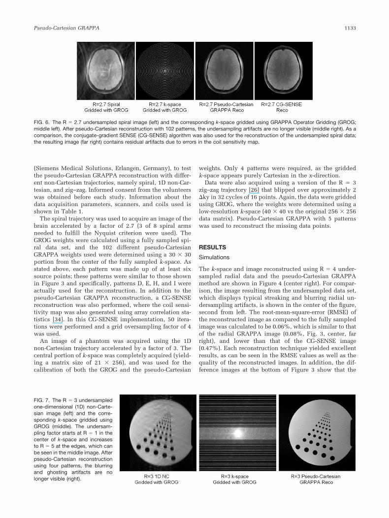
FIG. 6. The R � 2.7 undersampled spiral image (left) and the corresponding k-space gridded using GRAPPA Operator Gridding (GROG;middle left). After pseudo-Cartesian reconstruction with 102 patterns, the undersampling artifacts are no longer visible (middle right). As acomparison, the conjugate-gradient SENSE (CG-SENSE) algorithm was also used for the reconstruction of the undersampled spiral data;the resulting image (far right) contains residual artifacts due to errors in the coil sensitivity map.

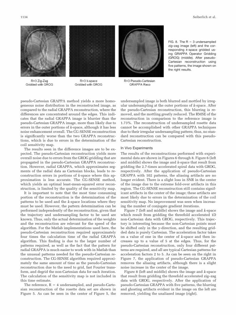
FIG. 7. The R � 3 undersampledone-dimensional (1D) non-Carte-sian image (left) and the corre-sponding k-space gridded usingGROG (middle). The undersam-pling factor starts at R � 1 in thecenter of k-space and increasesto R � 5 at the edges, which canbe seen in the middle image. Afterpseudo-Cartesian reconstructionusing four patterns, the blurringand ghosting artifacts are nolonger visible (right).

Pseudo-Cartesian GRAPPA 1133

pseudo-Cartesian GRAPPA method yields a more homo-geneous noise distribution in the reconstructed image, ascompared to the radial GRAPPA reconstruction, where thedifferences are concentrated around the edges. This indi-cates that the radial GRAPPA image is blurrier than thepseudo-Cartesian GRAPPA image, more than likely due toerrors in the outer portions of k-space, although it has lessnoise enhancement overall. The CG-SENSE reconstructionis significantly worse than the two GRAPPA reconstruc-tions, which is due to errors in the determination of thecoil sensitivity map.

The results seen in the difference images are to be ex-pected. The pseudo-Cartesian reconstruction yields moreoverall noise due to errors from the GROG gridding that arepropagated in the pseudo-Cartesian GRAPPA reconstruc-tion. However, radial GRAPPA, which approximates seg-ments of the radial data as Cartesian blocks, leads to re-construction errors in portions of k-space where this ap-proximation is less accurate. The CG-SENSE method,which yields an optimal least-mean-squared error recon-struction, is limited by the quality of the sensitivity map.

It is important to note that the most time consumingportion of the reconstruction is the determination of thepatterns to be used and the k-space locations where theymust be used. However, the pattern determination can beperformed independently of the reconstruction, given thatthe trajectory and undersampling factor to be used areknown. Thus, only the actual determination of the weightsand the reconstruction are relevant for the speed of thealgorithm. For the Matlab implementations used here, thepseudo-Cartesian reconstruction required approximatelyfour times the calculation time of the radial GRAPPAalgorithm. This finding is due to the larger number ofpatterns required, as well as the fact that the pattern forradial GRAPPA is much easier to work with in Matlab thanthe unusual patterns needed for the pseudo-Cartesian re-construction. The CG-SENSE algorithm required approxi-mately the same amount of time as the pseudo-Cartesianreconstruction due to the need to grid, fast Fourier trans-form, and degrid the non-Cartesian data for each iteration.The calculation of the sensitivity map is not included inthis time estimate.

The reference, R � 4 undersampled, and pseudo-Carte-sian reconstruction of the rosette data set are shown inFigure 5. As can be seen in the center of Figure 5, the

undersampled image is both blurred and mottled by irreg-ular undersampling at the outer portions of k-space. Afterthe pseudo-Cartesian reconstruction, this blurring is re-moved, and the mottling greatly reduced. The RMSE of thereconstruction in comparison to the reference image is1.73%. The reconstruction of undersampled rosette datacannot be accomplished with other GRAPPA techniquesdue to their irregular undersampling pattern; thus, no stan-dard reconstruction can be compared with this pseudo-Cartesian reconstruction.

In Vivo Experiments

The results of the reconstructions performed with experi-mental data are shown in Figures 6 through 8. Figure 6 (leftand middle) shows the image and k-space that result fromgridding the 2.7-times accelerated spiral data with GROG,respectively. After the application of pseudo-CartesianGRAPPA with 102 patterns, the aliasing artifacts are nolonger evident. There is a slight loss in SNR in the centerof the image due to the extreme fold-over artifacts in thisregion. The CG-SENSE reconstruction still contains signif-icant artifacts in the center of the image; these artifacts aremost likely due to errors in the determination of the coilsensitivity map. No improvement was seen when increas-ing the number of conjugate gradient iterations.

Figure 7 (left and middle) shows the image and k-spacewhich result from gridding the threefold accelerated 1Dnon-Cartesian data with GROG, respectively. This trajec-tory is interesting because the non-Cartesian points mustbe shifted only in the y-direction, and the resulting grid-ded data is purely Cartesian. The acceleration factor takeson a value of one in the center of k-space and then in-creases up to a value of 5 at the edges. Thus, for thepseudo-Cartesian reconstruction, only four different pat-terns are required, and all are typical Cartesian patterns foracceleration factors 2 to 5. As can be seen on the right inFigure 7, the application of pseudo-Cartesian GRAPPAremoves the aliasing artifacts, although there is a slightnoise increase in the center of the image.

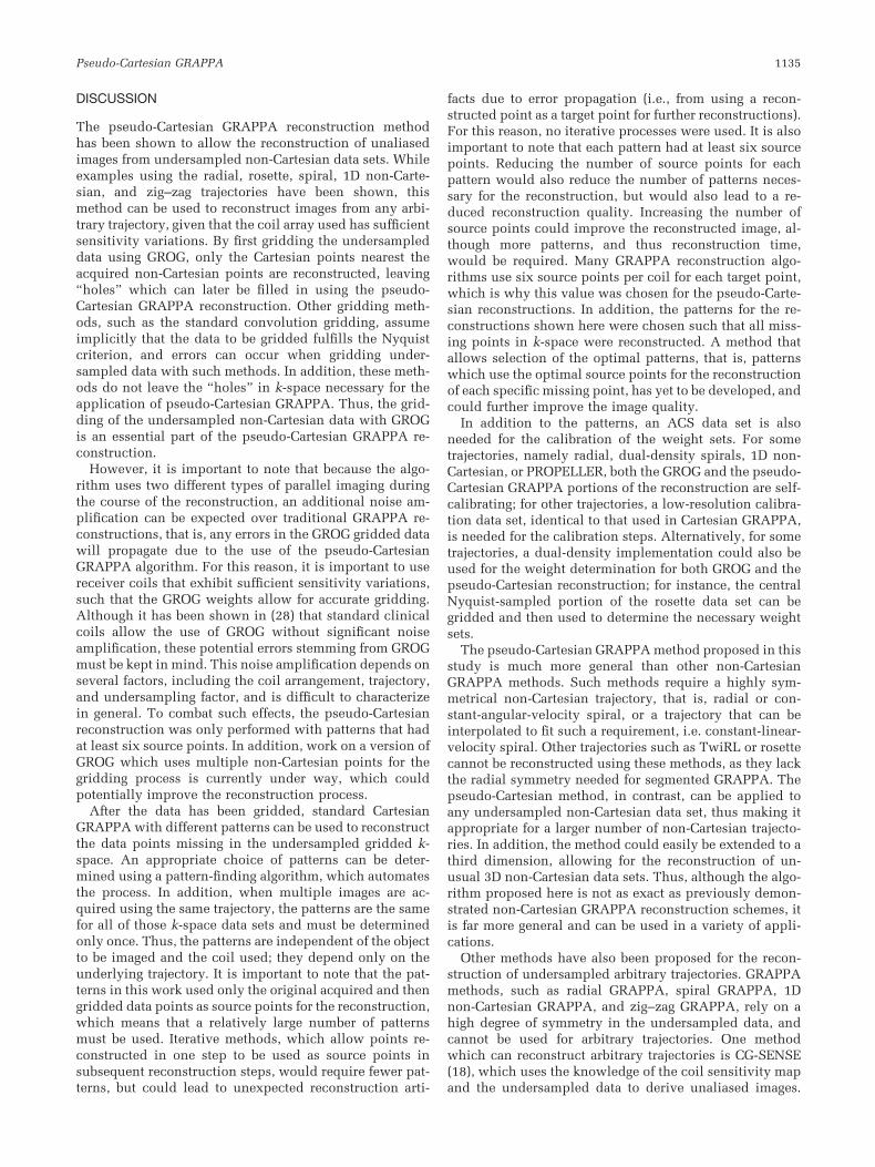
Figure 8 (left and middle) shows the image and k-spacethat result from gridding the threefold accelerated zig–zagdata with GROG, respectively. After the application ofpseudo-Cartesian GRAPPA with five patterns, the blurringand ghosting artifacts evident in the image on the left areremoved, yielding the unaliased image (right).

FIG. 8. The R � 3 undersampledzig–zag image (left) and the cor-responding k-space gridded us-ing GRAPPA Operator Gridding(GROG) (middle). After pseudo-Cartesian reconstruction usingfive patterns, the image shown onthe right results.

1134 Seiberlich et al.

DISCUSSION

The pseudo-Cartesian GRAPPA reconstruction methodhas been shown to allow the reconstruction of unaliasedimages from undersampled non-Cartesian data sets. Whileexamples using the radial, rosette, spiral, 1D non-Carte-sian, and zig–zag trajectories have been shown, thismethod can be used to reconstruct images from any arbi-trary trajectory, given that the coil array used has sufficientsensitivity variations. By first gridding the undersampleddata using GROG, only the Cartesian points nearest theacquired non-Cartesian points are reconstructed, leaving“holes” which can later be filled in using the pseudo-Cartesian GRAPPA reconstruction. Other gridding meth-ods, such as the standard convolution gridding, assumeimplicitly that the data to be gridded fulfills the Nyquistcriterion, and errors can occur when gridding under-sampled data with such methods. In addition, these meth-ods do not leave the “holes” in k-space necessary for theapplication of pseudo-Cartesian GRAPPA. Thus, the grid-ding of the undersampled non-Cartesian data with GROGis an essential part of the pseudo-Cartesian GRAPPA re-construction.

However, it is important to note that because the algo-rithm uses two different types of parallel imaging duringthe course of the reconstruction, an additional noise am-plification can be expected over traditional GRAPPA re-constructions, that is, any errors in the GROG gridded datawill propagate due to the use of the pseudo-CartesianGRAPPA algorithm. For this reason, it is important to usereceiver coils that exhibit sufficient sensitivity variations,such that the GROG weights allow for accurate gridding.Although it has been shown in (28) that standard clinicalcoils allow the use of GROG without significant noiseamplification, these potential errors stemming from GROGmust be kept in mind. This noise amplification depends onseveral factors, including the coil arrangement, trajectory,and undersampling factor, and is difficult to characterizein general. To combat such effects, the pseudo-Cartesianreconstruction was only performed with patterns that hadat least six source points. In addition, work on a version ofGROG which uses multiple non-Cartesian points for thegridding process is currently under way, which couldpotentially improve the reconstruction process.

After the data has been gridded, standard CartesianGRAPPA with different patterns can be used to reconstructthe data points missing in the undersampled gridded k-space. An appropriate choice of patterns can be deter-mined using a pattern-finding algorithm, which automatesthe process. In addition, when multiple images are ac-quired using the same trajectory, the patterns are the samefor all of those k-space data sets and must be determinedonly once. Thus, the patterns are independent of the objectto be imaged and the coil used; they depend only on theunderlying trajectory. It is important to note that the pat-terns in this work used only the original acquired and thengridded data points as source points for the reconstruction,which means that a relatively large number of patternsmust be used. Iterative methods, which allow points re-constructed in one step to be used as source points insubsequent reconstruction steps, would require fewer pat-terns, but could lead to unexpected reconstruction arti-

facts due to error propagation (i.e., from using a recon-structed point as a target point for further reconstructions).For this reason, no iterative processes were used. It is alsoimportant to note that each pattern had at least six sourcepoints. Reducing the number of source points for eachpattern would also reduce the number of patterns neces-sary for the reconstruction, but would also lead to a re-duced reconstruction quality. Increasing the number ofsource points could improve the reconstructed image, al-though more patterns, and thus reconstruction time,would be required. Many GRAPPA reconstruction algo-rithms use six source points per coil for each target point,which is why this value was chosen for the pseudo-Carte-sian reconstructions. In addition, the patterns for the re-constructions shown here were chosen such that all miss-ing points in k-space were reconstructed. A method thatallows selection of the optimal patterns, that is, patternswhich use the optimal source points for the reconstructionof each specific missing point, has yet to be developed, andcould further improve the image quality.

In addition to the patterns, an ACS data set is alsoneeded for the calibration of the weight sets. For sometrajectories, namely radial, dual-density spirals, 1D non-Cartesian, or PROPELLER, both the GROG and the pseudo-Cartesian GRAPPA portions of the reconstruction are self-calibrating; for other trajectories, a low-resolution calibra-tion data set, identical to that used in Cartesian GRAPPA,is needed for the calibration steps. Alternatively, for sometrajectories, a dual-density implementation could also beused for the weight determination for both GROG and thepseudo-Cartesian reconstruction; for instance, the centralNyquist-sampled portion of the rosette data set can begridded and then used to determine the necessary weightsets.

The pseudo-Cartesian GRAPPA method proposed in thisstudy is much more general than other non-CartesianGRAPPA methods. Such methods require a highly sym-metrical non-Cartesian trajectory, that is, radial or con-stant-angular-velocity spiral, or a trajectory that can beinterpolated to fit such a requirement, i.e. constant-linear-velocity spiral. Other trajectories such as TwiRL or rosettecannot be reconstructed using these methods, as they lackthe radial symmetry needed for segmented GRAPPA. Thepseudo-Cartesian method, in contrast, can be applied toany undersampled non-Cartesian data set, thus making itappropriate for a larger number of non-Cartesian trajecto-ries. In addition, the method could easily be extended to athird dimension, allowing for the reconstruction of un-usual 3D non-Cartesian data sets. Thus, although the algo-rithm proposed here is not as exact as previously demon-strated non-Cartesian GRAPPA reconstruction schemes, itis far more general and can be used in a variety of appli-cations.

Other methods have also been proposed for the recon-struction of undersampled arbitrary trajectories. GRAPPAmethods, such as radial GRAPPA, spiral GRAPPA, 1Dnon-Cartesian GRAPPA, and zig–zag GRAPPA, rely on ahigh degree of symmetry in the undersampled data, andcannot be used for arbitrary trajectories. One methodwhich can reconstruct arbitrary trajectories is CG-SENSE(18), which uses the knowledge of the coil sensitivity mapand the undersampled data to derive unaliased images.

Pseudo-Cartesian GRAPPA 1135

This method has three drawbacks: the first is that a sensi-tivity map is required, which can be difficult to generatefrom the non-Cartesian data, and the second is that theimage is reconstructed using an iterative conjugate gradi-ent method. Methods have been demonstrated which helpdetermine the stopping criteria for CG-SENSE (35), al-though many effects influence the selection of this value,including the trajectory, undersampling factor, coil arrayused, preconditioning, gridding method, and initial image.Thus, a direct reconstruction method which requires noadditional parameters, such as that proposed here, can beadvantageous. In addition, in dynamic imaging the itera-tive reconstruction has to be performed for each timeframe. In pseudo-Cartesian GRAPPA, the pattern andweights determination has to be performed only once andcan then be applied to the following time-frames leading toa fast data reconstruction.

A second reconstruction method that has been proposedfor arbitrarily sampled data is PARS (19,20), which per-forms a form of non-Cartesian SMASH using a sensitivitymap and the appropriate spatial harmonics to determinethe weight set needed to calculate each Cartesian point.The main drawback of PARS is that an extremely largenumber of weight sets must be calculated to reconstructthe image, as each non-Cartesian point generally requires adifferent weight set, which can become quite time-con-suming. Also, similar to CG-SENSE, coil sensitivity mapsmust be derived, which can be difficult in some imagingscenarios.

A third method is BOSCO (36), which first grids theundersampled data using standard convolution grid-ding, and then convolves the data a second time with aGRAPPA kernel, leading to an unaliased image. BOSCOhas only been demonstrated using spiral data, and suf-fers from the use of a single kernel, which could hamperthe reconstruction of other undersampled trajectories.Pseudo-Cartesian GRAPPA suffers from none of thesedrawbacks. It is not iterative, requires neither a sensi-tivity map nor an inordinately large number of weightsets, and the number of kernels used for the reconstruc-tion is not limited to one.

Finally, it is important to note that this method is baseddirectly on the conventional Cartesian GRAPPA method.In this sense, it is much more straightforward than othernon-Cartesian GRAPPA methods, which require dedicatedalgorithms. The combination of its simplicity and generalapplicability to many non-Cartesian trajectories makes thepseudo-Cartesian method in conjunction with GROG dem-onstrated here advantageous.

CONCLUSION

The pseudo-Cartesian GRAPPA reconstruction methodproposed here is a simple application of the basic Car-tesian GRAPPA algorithm to non-Cartesian data sets. Asthe algorithm uses the Cartesian patterns in griddedundersampled data for reconstruction, no additionalsegmentation or interpolation is necessary. In addition,for radial acquisitions, dual-density spirals, 1D non-Cartesian, or PROPELLER data, no additional ACS datamust be acquired as is needed for the standard GRAPPAreconstructions. However, the main strength of the

pseudo-Cartesian algorithm is that it can be applied toany undersampled non-Cartesian data set; this includesnot only radial and spiral trajectories, but also trajecto-ries which cannot be reconstructed using other non-Cartesian GRAPPA techniques, such as TwiRL and ro-sette. Because this algorithm can be applied to othernon-Cartesian trajectories, the need for a separate recon-struction procedure for each accelerated non-Cartesiantrajectory is eliminated.

REFERENCES

1. Sodickson DK, Manning WJ. Simultaneous acquisition of spatial har-monics (SMASH): fast imaging with radiofrequency coil arrays. MagnReson Med 1997;38:591–603.

2. Jakob PM, Griswold MA, Edelman RR, Sodickson DK. AUTO-SMASH:a self-calibrating technique for SMASH imaging. SiMultaneous Acqui-sition of Spatial Harmonics. MAGMA 1998;7:42–54.

3. Pruessmann KP, Weiger M, Scheidegger MB, Boesiger P. SENSE: sen-sitivity encoding for fast MRI. Magn Reson Med 1999;42:952–962.

4. Kyriakos WE, Panych LP, Kacher DF, Westin CF, Bao SM, Mulkern RV,Jolesz FA. Sensitivity profiles from an array of coils for encoding andreconstruction in parallel (SPACE RIP). Magn Reson Med 2000;44:301–308.

5. Griswold MA, Jakob PM, Nittka M, Goldfarb JW, Haase A. Partiallyparallel imaging with localized sensitivities (PILS). Magn Reson Med2000;44:602–609.

6. Heidemann RM, Griswold MA, Haase A, Jakob PM. VD-AUTO-SMASHimaging. Magn Reson Med 2001;45:1066–1074.

7. Bydder M, Larkman DJ, Hajnal JV. Generalized SMASH imaging. MagnReson Med 2002;47:160–170.

8. Griswold MA, Jakob PM, Heidemann RM, Nittka M, Jellus V, Wang J,Kiefer B, Haase A. Generalized autocalibrating partially parallel acqui-sitions (GRAPPA). Magn Reson Med 2002;47:1202–1210.

9. Ahn CB, Kim JH, Cho ZH. High-speed spiral-scan echo planar NMRimaging. IEEE Trans Med Imaging 1986;5:2–7.

10. Meyer CH, Hu BS, Nishimura DG, Macovski A. Fast spiral coronaryartery imaging. Magn Reson Med 1992;28:202–213.

11. Lauterbur PC. Image formation by induced local interactions: examplesemploying nuclear magnetic resonance. Nature (Lond) 1973;242:190–191.

12. Glover GH, Pauly JM. Projection reconstruction techniques for reduc-tion of motion effects in MRI. Magn Reson Med 1992;28:275–289.

13. Pipe JG. Motion-correction with PROPELLER MRI: application to headmotion and free-breathing cardiac imaging. Magn Reson Med 1999;42:963–969.

14. Busch M, Bornstedt A, Wendt M, Duerk JL, Lewin JS, Gronemeyer D.Fast “real time” imaging with different k-space update strategies forinterventional procedures. J Magn Reson Imaging 1998;8:944–954.

15. Noll DC. Multishot rosette trajectories for spectrally selective MR im-aging. IEEE Trans Med Imaging 1997;16:372–377.

16. Scheffler K, Hennig J. Reduced circular field-of-view imaging. MagnReson Med 1998;40:474–480.

17. Lauzon ML, Rutt BK. Effects of polar sampling in k-space. Magn ResonMed 1996;36:940–949.

18. Pruessmann KP, Weiger M, Boernert P, Boesiger P. Advances in sensi-tivity encoding with arbitrary k-space trajectories. Magn Reson Med2001;46:638–651.

19. Yeh EN, Stuber M, McKensie CA, Botnar RN, Leiner T, Ohliger MA,Grant AK, Willig-Onwuachi JD, Sodickson DK. Inherently self-calibrat-ing non-cartesian parallel imaging. Magn Reson Med 2005;54:1–8.

20. Samsonov AA, Block WF, Arunachalam A, Field AS. Advances inlocally constrained k-space-based parallel MRI. Magn Reson Med 2006;55:431–438.

21. Kannengiesser SAR, Noll TG. Towards a practical generalized imagereconstruction method for MRI. In: Proceedings of the 10th AnnualMeeting of the ISMRM, Honolulu, Hawaii, 2002. p. 155.

22. Griswold MA, Heidemann RM, Jakob PM. Direct parallel imaging re-construction of radially sampled data using GRAPPA with relativeshifts. In: Proceedings of the 11th Annual Meeting of the ISMRM,Toronto, Canada, 2003. p. 2349.

23. Heberlein K, Hu X. Auto-calibrated parallel spiral imaging. Magn Re-son Med 2006;55:619–625.

1136 Seiberlich et al.

24. Heidemann RM, Griswold MA, Seiberlich N, Kruger G, KannengiesserSA, Kiefer B, Wiggins G, Wald LL, Jakob PM. Direct parallel imagereconstructions for spiral trajectories using GRAPPA. Magn Reson Med2006;56:317–326.

25. Heidemann RM, Griswold MA, Seiberlich N, Nittka M, KannengiesserSA, Kiefer B, Jakob PM. Fast method for 1D non-cartesian parallelimaging using GRAPPA. Magn Reson Med 2007;57:1037–1046.

26. Breuer FA, Moriguchi H, Seiberlich N, Blaimer M, Duerk J, Jakob PM,Griswold MA. Zig-zag sampling for improved parallel imaging. In:Proceedings of the 23rd Annual Meeting of ESMRMB 2006, Warsaw,Poland, 2006. p. 301.

27. Nielsen HT , Olcott EW, Nishimura DG. Improved 2D time-of-flightangiography using a radial-line k-space acquisition. Magn Reson Med1997;37:285–291.

28. Seiberlich N, Breuer FA, Blaimer M, Barkauskas K, Jakob PM, GriswoldMA. Non-Cartesian data reconstruction using GRAPPA Operator Grid-ding (GROG). Magn Reson Med 2007;58:1257–1265.

29. Seiberlich N, Breuer FA, Blaimer M, Jakob PM, Griswold MA. Self-calibrated GRAPPA Operator Gridder (SC-GROG). In: Proceedings ofthe 15th Annual Meeting of the ISMRM, Berlin, Germany, 2007. p.153.

30. Jackson JI, Meyer CH, Nishimura DG, Macovski A. Selection of aconvolution function for Fourier inversion using gridding. IEEE TransMed Imaging 1991;10:473–478.

31. Seiberlich N, Heidemann RM, Breuer FA, Blaimer M, Griswold MA,Jakob PM. Pseudo-Cartesian GRAPPA reconstruction of undersamplednon-Cartesian data. In: Proceedings of the 14th Annual Meeting of theISMRM, Seattle, Washington, 2006. p. 2463.

32. Seiberlich N, Breuer FA, Heidemann RM, Blaimer M, Griswold MA,Jakob PM. Reconstruction of arbitrary non-Cartesian trajectories usingpseudo-Cartesian GRAPPA in conjunction with GRAPPA OperatorGridding (GROG). In: Proceedings of the 15th Annual Meeting of theISMRM, Miami, Florida, 2007. p. 334.

33. Arunachalam A, Samsonov A, Block WF. Self-calibrated GRAPPAmethod for 2D and 3D radial data. Magn Reson Med 2007;57:931–938.

34. Walsh DO, Gmitro AF, Marcellin MW. Adaptive reconstruction ofphased array MR imagery. Magn Reson Med 2000;43:682–690.

35. Qu P, Zhong K, Zhang B, Wang J, Shen GX. Convergence behavior ofiterative SENSE reconstruction with non-Cartesian trajectories. MagnReson Med 2005;54:1040–1045.

36. Hu P, Meyer CH. BOSCO: parallel image reconstruction based onsuccessive convolution operations. In: Proceedings of the 14th AnnualMeeting of the ISMRM, Seattle, Washington, 2006. p. 10.

Pseudo-Cartesian GRAPPA 1137