Embed Size (px)
Citation preview
AMATYC 2017 GeoGebra: A Tool to Connect S, T, and E with M 1 | P a g e
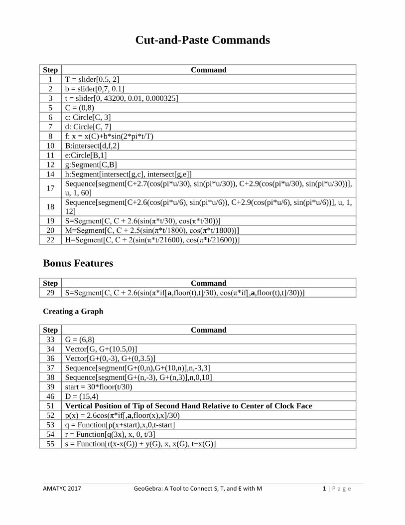
Cut-and-Paste Commands
Step Command
1 T = slider[0.5, 2]
2 b = slider[0,7, 0.1]
3 t = slider[0, 43200, 0.01, 0.000325]
5 C = (0,8)
6 c: Circle[C, 3]
7 d: Circle[C, 7]
8 f: x = x(C)+b*sin(2*pi*t/T)
10 B:intersect[d,f,2]
11 e:Circle[B,1]
12 g:Segment[C,B]
14 h:Segment[intersect[g,c], intersect[g,e]]
17 Sequence[segment[C+2.7(cos(pi*u/30), sin(pi*u/30)), C+2.9(cos(pi*u/30), sin(pi*u/30))],
u, 1, 60]
18 Sequence[segment[C+2.6(cos(pi*u/6), sin(pi*u/6)), C+2.9(cos(pi*u/6), sin(pi*u/6))], u, 1,
12]
19 S=Segment[C, C + 2.6(sin(π*t/30), cos(π*t/30))]
20 M=Segment[C, C + 2.5(sin(π*t/1800), cos(π*t/1800))]
22 H=Segment[C, C + 2(sin(π*t/21600), cos(π*t/21600))]
Bonus Features
Step Command
29 S=Segment[C, C + 2.6(sin(π*if[a,floor(t),t]/30), cos(π*if[,a,floor(t),t]/30))]
Creating a Graph
Step Command
33 G = (6,8)
34 Vector[G, G+(10.5,0)]
36 Vector[G+(0,-3), G+(0,3.5)]
37 Sequence[segment[G+(0,n),G+(10,n)],n,-3,3]
38 Sequence[segment[G+(n,-3), G+(n,3)],n,0,10]
39 start = 30*floor(t/30)
46 D = (15,4)
51 Vertical Position of Tip of Second Hand Relative to Center of Clock Face
52 p(x) = 2.6cos(π*if[,a,floor(x),x]/30)
53 q = Function[p(x+start),x,0,t-start]
54 r = Function[q(3x), x, 0, t/3]
55 s = Function[r(x-x(G)) + y(G), x, x(G), t+x(G)]
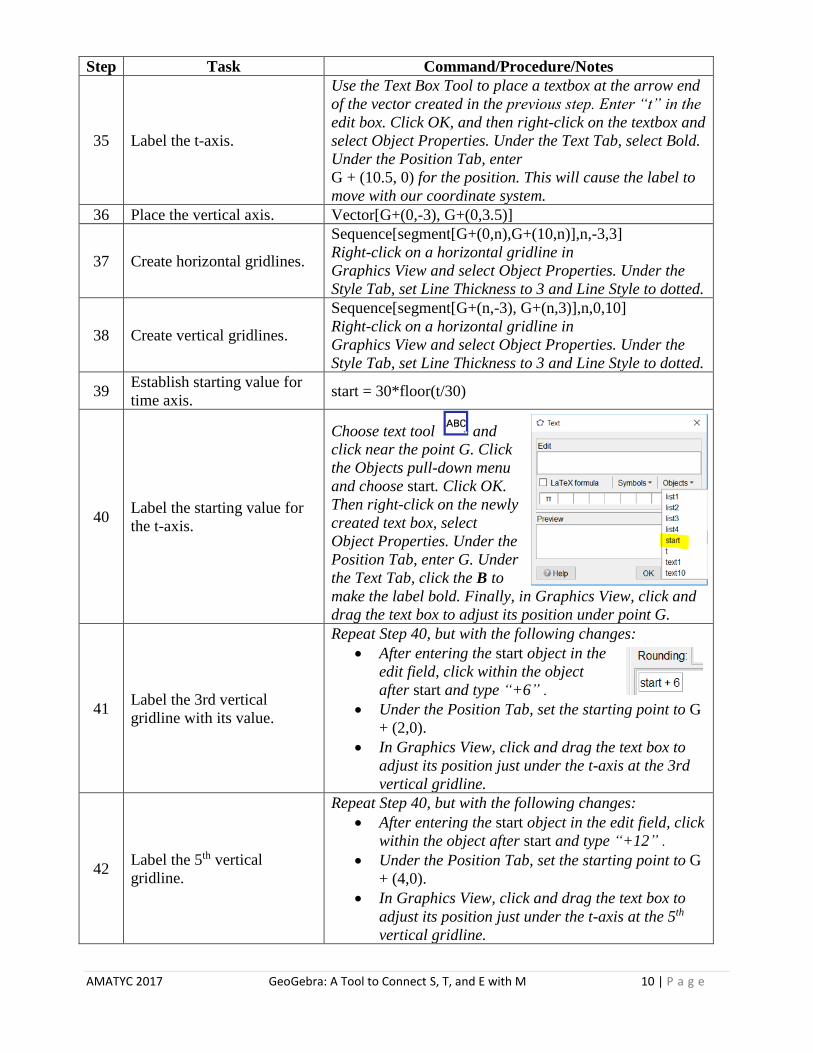
A Tool to Connect S, T, and E with M
Christopher Heeren
American River College

AMATYC 2017 GeoGebra: A Tool to Connect S, T, and E with M 2 | P a g e
AMATYC 2017 GeoGebra: A Tool to Connect S, T, and E with M 3 | P a g e
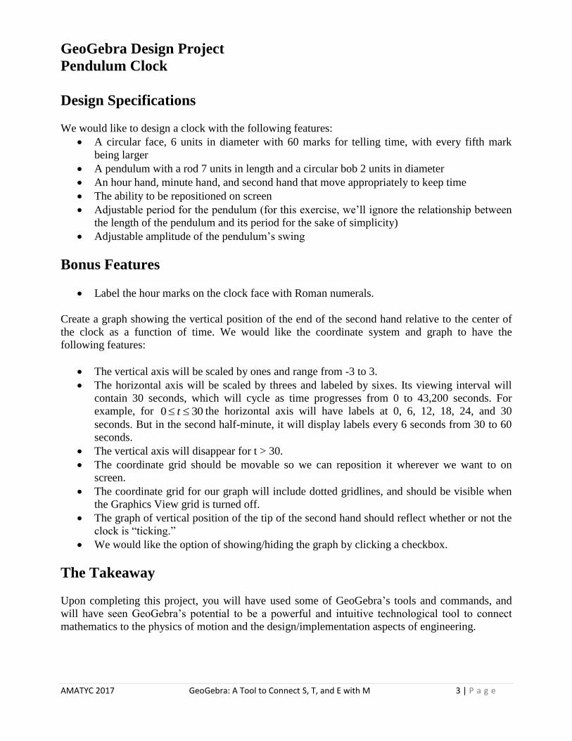
GeoGebra Design Project
Pendulum Clock
Design Specifications
We would like to design a clock with the following features:
• A circular face, 6 units in diameter with 60 marks for telling time, with every fifth mark
being larger
• A pendulum with a rod 7 units in length and a circular bob 2 units in diameter
• An hour hand, minute hand, and second hand that move appropriately to keep time
• The ability to be repositioned on screen
• Adjustable period for the pendulum (for this exercise, we’ll ignore the relationship between
the length of the pendulum and its period for the sake of simplicity)
• Adjustable amplitude of the pendulum’s swing
Bonus Features
• Label the hour marks on the clock face with Roman numerals.
Create a graph showing the vertical position of the end of the second hand relative to the center of
the clock as a function of time. We would like the coordinate system and graph to have the
following features:
• The vertical axis will be scaled by ones and range from -3 to 3.
• The horizontal axis will be scaled by threes and labeled by sixes. Its viewing interval will
contain 30 seconds, which will cycle as time progresses from 0 to 43,200 seconds. For
example, for 0 30t the horizontal axis will have labels at 0, 6, 12, 18, 24, and 30
seconds. But in the second half-minute, it will display labels every 6 seconds from 30 to 60
seconds.
• The vertical axis will disappear for t > 30.
• The coordinate grid should be movable so we can reposition it wherever we want to on
screen.
• The coordinate grid for our graph will include dotted gridlines, and should be visible when
the Graphics View grid is turned off.
• The graph of vertical position of the tip of the second hand should reflect whether or not the
clock is “ticking.”
• We would like the option of showing/hiding the graph by clicking a checkbox.
The Takeaway
Upon completing this project, you will have used some of GeoGebra’s tools and commands, and
will have seen GeoGebra’s potential to be a powerful and intuitive technological tool to connect
mathematics to the physics of motion and the design/implementation aspects of engineering.
AMATYC 2017 GeoGebra: A Tool to Connect S, T, and E with M 4 | P a g e
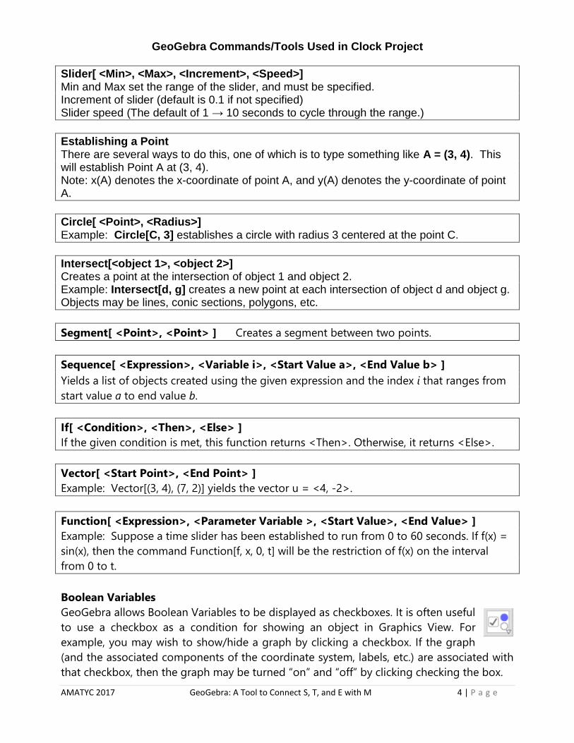
GeoGebra Commands/Tools Used in Clock Project
Slider[ <Min>, <Max>, <Increment>, <Speed>] Min and Max set the range of the slider, and must be specified. Increment of slider (default is 0.1 if not specified) Slider speed (The default of 1 → 10 seconds to cycle through the range.)
Establishing a Point There are several ways to do this, one of which is to type something like A = (3, 4). This will establish Point A at (3, 4). Note: x(A) denotes the x-coordinate of point A, and y(A) denotes the y-coordinate of point A.
Circle[ <Point>, <Radius>] Example: Circle[C, 3] establishes a circle with radius 3 centered at the point C.
Intersect[<object 1>, <object 2>] Creates a point at the intersection of object 1 and object 2. Example: Intersect[d, g] creates a new point at each intersection of object d and object g. Objects may be lines, conic sections, polygons, etc.
Segment[ <Point>, <Point> ] Creates a segment between two points.
Sequence[ <Expression>, <Variable i>, <Start Value a>, <End Value b> ]
Yields a list of objects created using the given expression and the index i that ranges from
start value a to end value b.
If[ <Condition>, <Then>, <Else> ]
If the given condition is met, this function returns <Then>. Otherwise, it returns <Else>.
Vector[ <Start Point>, <End Point> ]
Example: Vector[(3, 4), (7, 2)] yields the vector u = <4, -2>.
Function[ <Expression>, <Parameter Variable >, <Start Value>, <End Value> ]
Example: Suppose a time slider has been established to run from 0 to 60 seconds. If f(x) =
sin(x), then the command Function[f, x, 0, t] will be the restriction of f(x) on the interval
from 0 to t.
Boolean Variables
GeoGebra allows Boolean Variables to be displayed as checkboxes. It is often useful
to use a checkbox as a condition for showing an object in Graphics View. For
example, you may wish to show/hide a graph by clicking a checkbox. If the graph
(and the associated components of the coordinate system, labels, etc.) are associated with
that checkbox, then the graph may be turned “on” and “off” by clicking checking the box.
AMATYC 2017 GeoGebra: A Tool to Connect S, T, and E with M 5 | P a g e
GeoGebra: A Tool to Connect S, T, and E with M
Abstract It is common for mathematics students to encounter challenges when attempting to solve word
problems, particularly those involving motion. Physics students often develop a deeper
understanding of mathematics when they see it in action, and engineering students similarly solidify
their grasp of mathematical concepts as they design things. GeoGebra allows students to both see
and design. Instructors can help their developmental students approach application problems by
showing them a dynamic model. More advanced students can design such models themselves. If
you have yet to explore GeoGebra, this mini-course may provide just the nudge you need to begin
discovering its power and utility.
Our Project To illustrate some of the features of GeoGebra and to get a sense of its usefulness in connecting
mathematics to other STEM areas, we’ll build a pendulum clock.
Setup
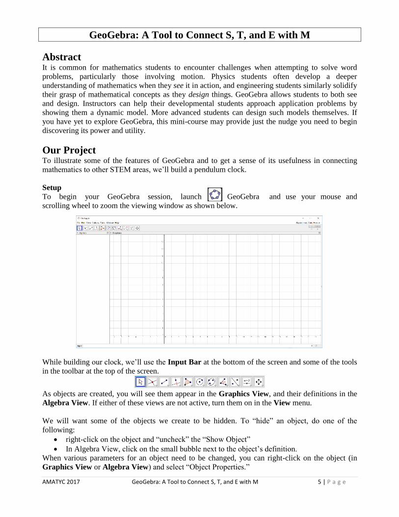
To begin your GeoGebra session, launch GeoGebra and use your mouse and
scrolling wheel to zoom the viewing window as shown below.
While building our clock, we’ll use the Input Bar at the bottom of the screen and some of the tools
in the toolbar at the top of the screen.
As objects are created, you will see them appear in the Graphics View, and their definitions in the
Algebra View. If either of these views are not active, turn them on in the View menu.
We will want some of the objects we create to be hidden. To “hide” an object, do one of the
following:
• right-click on the object and “uncheck” the “Show Object”
• In Algebra View, click on the small bubble next to the object’s definition.
When various parameters for an object need to be changed, you can right-click on the object (in
Graphics View or Algebra View) and select “Object Properties.”
AMATYC 2017 GeoGebra: A Tool to Connect S, T, and E with M 6 | P a g e
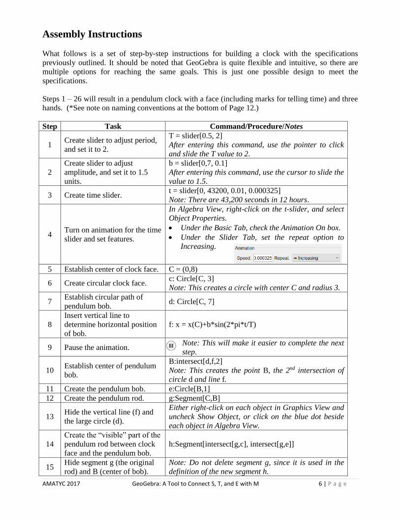
Assembly Instructions
What follows is a set of step-by-step instructions for building a clock with the specifications
previously outlined. It should be noted that GeoGebra is quite flexible and intuitive, so there are
multiple options for reaching the same goals. This is just one possible design to meet the
specifications.
Steps 1 – 26 will result in a pendulum clock with a face (including marks for telling time) and three
hands. (*See note on naming conventions at the bottom of Page 12.)
Step Task Command/Procedure/Notes
1 Create slider to adjust period,
and set it to 2.
T = slider[0.5, 2]
After entering this command, use the pointer to click
and slide the T value to 2.
2
Create slider to adjust
amplitude, and set it to 1.5
units.
b = slider[0,7, 0.1]
After entering this command, use the cursor to slide the
value to 1.5.
3 Create time slider. t = slider[0, 43200, 0.01, 0.000325]
Note: There are 43,200 seconds in 12 hours.
4 Turn on animation for the time
slider and set features.
In Algebra View, right-click on the t-slider, and select
Object Properties.
• Under the Basic Tab, check the Animation On box.
• Under the Slider Tab, set the repeat option to
Increasing.
5 Establish center of clock face. C = (0,8)
6 Create circular clock face. c: Circle[C, 3]
Note: This creates a circle with center C and radius 3.
7 Establish circular path of
pendulum bob. d: Circle[C, 7]
8
Insert vertical line to
determine horizontal position
of bob.
f: x = x(C)+b*sin(2*pi*t/T)
9 Pause the animation. Note: This will make it easier to complete the next
step.
10 Establish center of pendulum
bob.
B:intersect[d,f,2]
Note: This creates the point B, the 2nd intersection of
circle d and line f.
11 Create the pendulum bob. e:Circle[B,1]
12 Create the pendulum rod. g:Segment[C,B]
13 Hide the vertical line (f) and
the large circle (d).
Either right-click on each object in Graphics View and
uncheck Show Object, or click on the blue dot beside
each object in Algebra View.
14
Create the “visible” part of the
pendulum rod between clock
face and the pendulum bob.
h:Segment[intersect[g,c], intersect[g,e]]
15 Hide segment g (the original
rod) and B (center of bob).
Note: Do not delete segment g, since it is used in the
definition of the new segment h.

AMATYC 2017 GeoGebra: A Tool to Connect S, T, and E with M 7 | P a g e
Step Task Command/Procedure/Notes
16 Start the animation. Click the icon in the lower left corner. You
should see your clock come to life!
17 Place the 60 “minute” marks
on the clock face.
Sequence[segment[C+2.7(cos(pi*u/30), sin(pi*u/30)),
C+2.9(cos(pi*u/30), sin(pi*u/30))], u, 1, 60]
18 Place 12 larger “hour” marks
on the clock face.
Sequence[segment[C+2.6(cos(pi*u/6), sin(pi*u/6)),
C+2.9(cos(pi*u/6), sin(pi*u/6))], u, 1, 12]
Right-click on list2 in Algebra View and select Object
Properties. Under the Style Tab, adjust the Line
Thickness to 7.
19 Create the second hand.
S=Segment[C, C + 2.6(sin(π*t/30), cos(π*t/30))]
Note: The use of sine in the x-coordinate and cosine in
the y-coordinate cause the hand of the clock to start in
the 12 o’clock position and rotate clockwise as the time
parameter t increases.
20 Create the minute hand. M=Segment[C, C + 2.5(sin(π*t/1800), cos(π*t/1800))]
21 Change thickness of minute
hand.
Right-click on M in Algebra View and select Object
Properties. Under the Style Tab, adjust the Line
Thickness to 8.
22 Create the hour hand. H=Segment[C, C + 2(sin(π*t/21600), cos(π*t/21600))]
23 Change thickness of hour
hand.
Right-click on H in Algebra View and select Object
Properties. Under the Style Tab, adjust the Line
Thickness to 13.
24
Clean up your workspace.
(It might help to pause the
animation to complete the next
few steps.)
Select the Show/Hide Label tool. Then,
in Graphics View, click on the
following objects to hide their labels:
• C (center of clock face)
• c (circular clock face)
• H (hour hand)
• M (minute hand)
• S (second hand)
• h (visible part of rod)
• e (circular pendulum bob)
Right-click on a blank location in Graphics View to
turn off the Axes and the Grid.
25 Affix the “brand name” to the
clock face.
Choose the Text tool, and click below the
center of the clock face. Enter text for the
“brand name” of your choice (maybe
“GeoGebra”). Then right-click on your
new text object, and select Object
Properties. Under the Position Tab, use
the pulldown menu to select C. Then click
on the text object and drag it to the desired
position. Note: This process of formatting the position
of the text object will allow it to move with the clock.
26 “Polish” your clock.
Right-click on any objects you desire, and select Object
Properties. Under the Color Tab, choose colors and
adjust opacity as desired.
AMATYC 2017 GeoGebra: A Tool to Connect S, T, and E with M 8 | P a g e
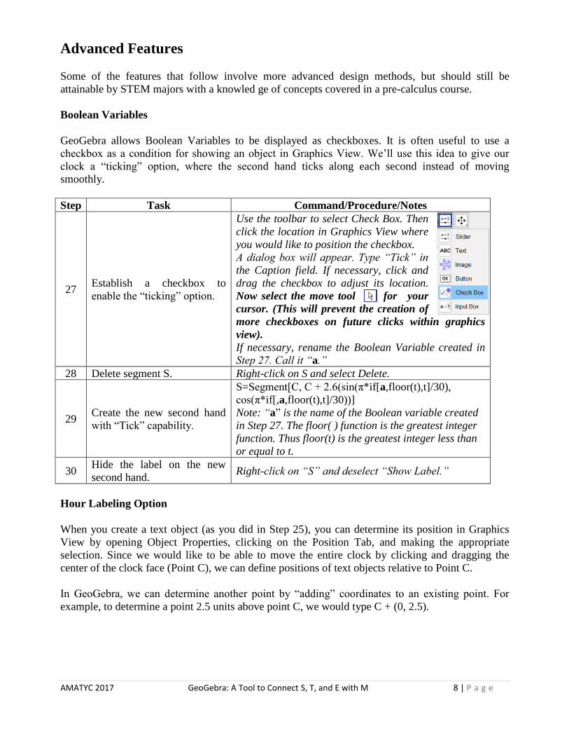
Advanced Features
Some of the features that follow involve more advanced design methods, but should still be
attainable by STEM majors with a knowled ge of concepts covered in a pre-calculus course.
Boolean Variables
GeoGebra allows Boolean Variables to be displayed as checkboxes. It is often useful to use a
checkbox as a condition for showing an object in Graphics View. We’ll use this idea to give our
clock a “ticking” option, where the second hand ticks along each second instead of moving
smoothly.
Step Task Command/Procedure/Notes
27 Establish a checkbox to
enable the “ticking” option.
Use the toolbar to select Check Box. Then
click the location in Graphics View where
you would like to position the checkbox.
A dialog box will appear. Type “Tick” in
the Caption field. If necessary, click and
drag the checkbox to adjust its location.
Now select the move tool for your
cursor. (This will prevent the creation of
more checkboxes on future clicks within graphics
view).
If necessary, rename the Boolean Variable created in
Step 27. Call it “a.”
28 Delete segment S. Right-click on S and select Delete.
29 Create the new second hand
with “Tick” capability.
S=Segment[C, C + 2.6(sin(π*if[a,floor(t),t]/30),
cos(π*if[,a,floor(t),t]/30))]
Note: “a” is the name of the Boolean variable created
in Step 27. The floor( ) function is the greatest integer
function. Thus floor(t) is the greatest integer less than
or equal to t.
30 Hide the label on the new
second hand. Right-click on “S” and deselect “Show Label.”
Hour Labeling Option
When you create a text object (as you did in Step 25), you can determine its position in Graphics
View by opening Object Properties, clicking on the Position Tab, and making the appropriate
selection. Since we would like to be able to move the entire clock by clicking and dragging the
center of the clock face (Point C), we can define positions of text objects relative to Point C.
In GeoGebra, we can determine another point by “adding” coordinates to an existing point. For
example, to determine a point 2.5 units above point C, we would type C + (0, 2.5).
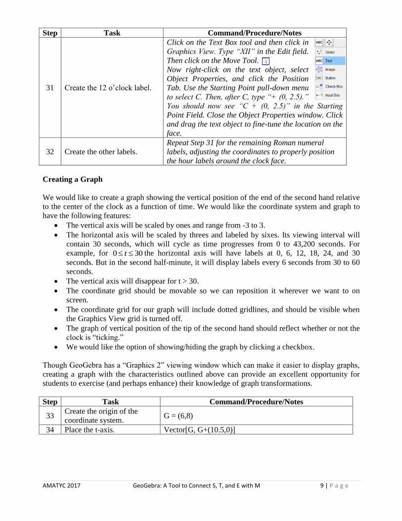
AMATYC 2017 GeoGebra: A Tool to Connect S, T, and E with M 9 | P a g e
Step Task Command/Procedure/Notes
31 Create the 12 o’clock label.
Click on the Text Box tool and then click in
Graphics View. Type “XII” in the Edit field.
Then click on the Move Tool.
Now right-click on the text object, select
Object Properties, and click the Position
Tab. Use the Starting Point pull-down menu
to select C. Then, after C, type “+ (0, 2.5).”
You should now see “C + (0, 2.5)” in the Starting
Point Field. Close the Object Properties window. Click
and drag the text object to fine-tune the location on the
face.
32 Create the other labels.
Repeat Step 31 for the remaining Roman numeral
labels, adjusting the coordinates to properly position
the hour labels around the clock face.
Creating a Graph
We would like to create a graph showing the vertical position of the end of the second hand relative
to the center of the clock as a function of time. We would like the coordinate system and graph to
have the following features:
• The vertical axis will be scaled by ones and range from -3 to 3.
• The horizontal axis will be scaled by threes and labeled by sixes. Its viewing interval will
contain 30 seconds, which will cycle as time progresses from 0 to 43,200 seconds. For
example, for 0 30t the horizontal axis will have labels at 0, 6, 12, 18, 24, and 30
seconds. But in the second half-minute, it will display labels every 6 seconds from 30 to 60
seconds.
• The vertical axis will disappear for t > 30.
• The coordinate grid should be movable so we can reposition it wherever we want to on
screen.
• The coordinate grid for our graph will include dotted gridlines, and should be visible when
the Graphics View grid is turned off.
• The graph of vertical position of the tip of the second hand should reflect whether or not the
clock is “ticking.”
• We would like the option of showing/hiding the graph by clicking a checkbox.
Though GeoGebra has a “Graphics 2” viewing window which can make it easier to display graphs,
creating a graph with the characteristics outlined above can provide an excellent opportunity for
students to exercise (and perhaps enhance) their knowledge of graph transformations.
Step Task Command/Procedure/Notes
33 Create the origin of the
coordinate system. G = (6,8)
34 Place the t-axis. Vector[G, G+(10.5,0)]
AMATYC 2017 GeoGebra: A Tool to Connect S, T, and E with M 10 | P a g e
Step Task Command/Procedure/Notes
35 Label the t-axis.
Use the Text Box Tool to place a textbox at the arrow end
of the vector created in the previous step. Enter “t” in the
edit box. Click OK, and then right-click on the textbox and
select Object Properties. Under the Text Tab, select Bold.
Under the Position Tab, enter
G + (10.5, 0) for the position. This will cause the label to
move with our coordinate system.
36 Place the vertical axis. Vector[G+(0,-3), G+(0,3.5)]
37 Create horizontal gridlines.
Sequence[segment[G+(0,n),G+(10,n)],n,-3,3]
Right-click on a horizontal gridline in
Graphics View and select Object Properties. Under the
Style Tab, set Line Thickness to 3 and Line Style to dotted.
38 Create vertical gridlines.
Sequence[segment[G+(n,-3), G+(n,3)],n,0,10]
Right-click on a horizontal gridline in
Graphics View and select Object Properties. Under the
Style Tab, set Line Thickness to 3 and Line Style to dotted.
39 Establish starting value for
time axis. start = 30*floor(t/30)
40 Label the starting value for
the t-axis.
Choose text tool and
click near the point G. Click
the Objects pull-down menu
and choose start. Click OK.
Then right-click on the newly
created text box, select
Object Properties. Under the
Position Tab, enter G. Under
the Text Tab, click the B to
make the label bold. Finally, in Graphics View, click and
drag the text box to adjust its position under point G.
41 Label the 3rd vertical
gridline with its value.
Repeat Step 40, but with the following changes:
• After entering the start object in the
edit field, click within the object
after start and type “+6” .
• Under the Position Tab, set the starting point to G
+ (2,0).
• In Graphics View, click and drag the text box to
adjust its position just under the t-axis at the 3rd
vertical gridline.
42 Label the 5th vertical
gridline.
Repeat Step 40, but with the following changes:
• After entering the start object in the edit field, click
within the object after start and type “+12” .
• Under the Position Tab, set the starting point to G
+ (4,0).
• In Graphics View, click and drag the text box to
adjust its position just under the t-axis at the 5th
vertical gridline.
AMATYC 2017 GeoGebra: A Tool to Connect S, T, and E with M 11 | P a g e
Step Task Command/Procedure/Notes
43 Label the 7th vertical
gridline.
Repeat Step 40, but with the following changes:
• After entering the start object in the edit field, click
within the object after start and type “+18” .
• Under the Position Tab, set the starting point to G
+ (6,0).
• In Graphics View, click and drag the text box to
adjust its position just under the t-axis at the 7th
vertical gridline.
44 Label the 9th vertical
gridline.
Repeat Step 40, but with the following changes:
• After entering the start object in the edit field, click
within the object after start and type “+24” .
• Under the Position Tab, set the starting point to G
+ (8,0).
In Graphics View, click and drag the text box to adjust its
position just under the t-axis at the 9th vertical gridline.
45 Label the 11th vertical
gridline.
Repeat Step 40, but with the following changes:
• After entering the start object in the edit field, click
within the object after start and type “+30” .
• Under the Position Tab, set the starting point to G
+ (10,0).
In Graphics View, click and drag the text box to adjust its
position just under the t-axis at the 11th vertical gridline.
46 Create a “handle” for
moving the coordinate grid.
D = (15,4)
This will establish a new point D near the bottom-right
corner of your coordinate grid. In Object Properties, set
the point size to 7, and the Points Style to diamond-
shaped.
47 Redefine Point G.
In Graphics View, double-click on Point G. In the
Redefine box, enter D+(-10, 3) and click OK.
Now try clicking and dragging Point D. You should see
the entire coordinate system move with Point D.
48 Cleanup the coordinate
system.
Select the Show/Hide Label tool and then click on
each axis, and Point D to hide their labels.
49 Scale the vertical axis.
Use the Text Tool to create a text box containing “-3” and
set it’s position to G + (0, -3) and style to bold. Click and
drag the text box to adjust its postion appropriately.
50 Scale the vertical axis.
(continued)
Use the Text Tool to create a text box containing “-3” and
set it’s position to G + (0, 3) and style to bold. Click and
drag the text box to adjust its postion appropriately.
51 Label the graph.
Use the Text Tool to create a text box containing the title
“Vertical Position of Tip of Second Hand Relative to
Center of Clock Face”
Position the text box at G + (0, 3.5).
52
Define function p(x) as the
vertical position of the tip of
the second hand. (See Step
29.)
p(x) = 2.6cos(π*if[,a,floor(x),x]/30)
AMATYC 2017 GeoGebra: A Tool to Connect S, T, and E with M 12 | P a g e
Step Task Command/Procedure/Notes
53
Shift the graph of p(t) to the
left by “start” units and
restrict the domain to the
interval
start x t .
q = Function[p(x+start),x,0,t-start]
54 Compress the graph
horizontally by a factor of 3. r = Function[q(3x), x, 0, t/3]
55
Shift the graph of r(t) right
x(G) units and up y(G) units
to place it in the coordinate
grid.
s = Function[r(x-x(G)) + y(G), x, x(G), t+x(G)]
Open Object Properties and choose a color and style
(thickness) for this graph.
56 Clean up the Graphics View.
Hide the functions p, q and r.
Hide Point G.
Hide the label on function s.
57 Establish a checkbox for
showing/hiding the graph.
Use the Checkbox Tool to place a textbox below the
“Tick” checkbox. Enter “Graph” in the caption field.
(This should create a Boolean Variable i. If named
differently, rename it i to facilitate Steps 58 and 59.)
58
Associate all parts of the
coordinate system with the
checkbox.
Right-click and drag a box around the entire coordinate
system. Then right-click within this area and open Object
Properties. Under the Advanced Tab, in the Condition to
Show Object field, enter “i.”
59 Cause the vertical axis to
disappear for t > 30 seconds.
Right-click on the vertical axis (vector v) and select
Object Properties. Under the Advanced Tab, enter 30i t
Note: is the logical AND symbol. When you click in the
Condition to Show Object field, you will see a small
symbol at the far right. Click on this to view a menu
of symbols, and select .
Further Considerations
1. In reality, the period of a pendulum is related to its length. Research this relationship. How
might you modify your clock design to accurately reflect this relationship between period
and length?
2. Steps 52-55 were used to create the graph for the vertical position of the tip of the second
hand with respect to time relative to the center of the clock face. Can you find a single
function that would replace functions p, q, r and s?
*Note: GeoGebra has naming conventions for naming new objects automatically. For example,
entering “Circle[(0,0), 4]” in the input bar will create a circle of radius 4 centered at the origin, and
GeoGebra will choose its name. However, entering “c:Circle[(0,0), 4]” will create the same circle,
but will give it the name “c.” Using this method, we can override the default naming conventions,
and control the names given to objects as we create them.


