1

Nanoindentation Testing of Gear Steels

A. Oila and S.J. Bull

School of Chemical Engineering and Advanced Materials

University of Newcastle, Newcastle upon Tyne, NE1 7RU, UK.

Abstract

A combination of nanoindentation testing and AFM has been used to accurately

determine the hardness and elastic modulus of gear steels. The results confirmed that the

conventional analysis method due to Oliver and Pharr tends to greatly overestimate the

hardness and elastic modulus due to the effect of pile-up by about 25%. Hardness and

Young’s modulus calculated using the slopes method are overestimated by about 10%.

AFM offers a reliable method for measuring area of contact because the indentations are

relatively well defined in gear steel samples. Two correction factors, 82.0Hk and

75.0Ek have been determined and applied in the Oliver and Pharr formulas for

hardness and elastic modulus respectively. The corrected values are in good agreement

with those expected.

1. Introduction

The main mechanisms by which gears fail in service are tooth bending fatigue and

surface contact fatigue. Bending stresses lead to crack initiation at the root of the tooth

and contact stresses induce shear stresses in the near-surface regions, which lead to

crack initiation in this zone. Therefore a steel used for gear manufacturing must provide

enhanced ductility in the core to withstand the bending stresses developed there and a

hard tooth surface to resist the shear stresses developed at and near below the surface

[1]. The depth of maximum shear stress is located, depending on the elastic properties

of steel and gear geometry at about 0.18-0.3mm below the surface [2].

In order to achieve these requirements steel gears are usually subjected to

thermochemical treatments such as carburising or nitriding for enhancing the

mechanical properties of a thin surface layer. According to Cram [3] the case depth

should be at least twice the depth of the point of maximum shear stress in order to

prevent high local stress concentration. Microindentation testing is often used to

monitor the thickness and hardness of this case.

The case microstructure of a carburised, quenched and tempered steel consists of

tempered martensite, retained austenite and carbides, meanwhile the microstructure of

the surface layer of a nitrided steel consists of nitrides, carbides and carbonitrides

formed with iron and alloying elements. The regions of retained austenite in carburised

steels are sufficiently small (<10 microns) that only nanoindentation can be used to

reliably measure their properties in correctly processed gears. In nitrided gears the

carbonitrides, which form in the nitrogen diffusion layer may have a higher hardness

2

and modulus than the surrounding steel. Moreover, in fatigued specimens phase

transformations take place. The mechanisms of these transformations as well as the

properties of the new phases are not very well understood, yet. Because of these

complex microstructures containing different phases the classical method of measuring

Vickers microhardness at moderate load (usually~3N) gives only an average material

response which does not fully characterise the surface. Nanoindentation allows more

localised measurements that directly relate to the mechanical properties of individual

microstructural features.

However, the conventional analysis method to extract hardness and modulus from

nanoindentation data due to Oliver and Pharr [4] tends to greatly overestimate the

hardness and modulus due to the effect of “pile-up” (Figure 1). The material displaced

by the indenter pushes out to the sides of the indentation and forms a pile-up which

supports some of the load, making the projected contact area larger than the cross-

sectional area of the indenter at the original surface level.

The Oliver and Pharr method, which is based upon relationships developed by Snedon

[5] for the penetration of an elastic half space by indenters that can be described as

solids of revolution of a smooth function gives Equations (1)-(4) for hardness and

Young’s modulus calculation.

cA

PH max (1)

c

rA

SE

2 (2)

i

i

r EEE

22 111

(3)

S

Pc

maxmax (4)

where H is hardness, maxP the maximum indentation load, 2cc CA is the projected

area of tip-sample contact, C =constant of the area function (C=24.56 for a perfect

Berkovich indenter), rE the reduced modulus, dhdPS represents the experimentally

measured stiffness (the slope of the unloading curve evaluated at the position of

maximum load), P is the indenter load, h is the penetration depth, a dimensionless

parameter related to the geometry of the indenter ( 034.1 for a triangular punch), is

a correction factor introduced by Hay et al. [6] due to unrealistic boundary conditions

used by Snedon, iEE and are the Young’s moduli of sample and indenter, i and are

the Poisson’s ratios of sample and indenter respectively, is a constant assumed to be

0.75. This procedure can be successfully applied for materials with a high work

hardening exponent which sink-in during indentation but for highly plastic materials

like steels this procedure may cause significant errors due to piling-up phenomenon [7].

3

A second source of error in processing nanoindentation data relates to the deviation of

the geometry of the indenter from its intended shape. Recently, Oliver [8] suggested a

new technique called “the slope technique”, for calculating hardness, modulus and

contact area from indentation data, which substantially diminishes this effect but does

not eliminate the effect of pile-up. The slope technique is based upon the Equations (5)

and (6): 2

2

1

lu

lu

SS

SS

CPH

(5)

lu

lur

SS

SS

PCE

22

12

(6)

where P is the indentation load, lS and uS are the slopes of the loading and unloading

curves respectively. This approach has been previously shown to be less sensitive to the

effects of pile-up [9].

2. Experimental

2.1. Samples

In the present study two different gear steels have been tested: 20MnCr5 carburised

steel and EN40B nitrided steel. The chemical compositions of the two steels are given

in Table1. The specimens examined in this study were cut from gear teeth (20MnCr5

carburised and EN40B nitrided) and polished on a cross section perpendicular to the

treated surface to a high surface finish using SiC paper followed by 1m diamond paste

in order to reduce the scattering of nanoindentation data caused by surface roughness.

The specimens were initially nickel plated in order to ensure edge retention during

polishing. The microstructure of the specimens has been observed by scanning electron

microscopy (SEM) without etching and by reflected light microscope, after etching the

surface with 2% Nital.

2.2. Nanoindentation tests

Nanoindentation tests were performed using a Nano Indenter IITM

manufactured by

Nano Instruments, Knoxville, TN, USA. To determine the effects of pile-up on hardness

measured by nanoindentation a range of indentations were made in the core region of

the nitrided steel (EN40B) using peak loads from 1mN to 500mN. Ten indentations

were performed at each load. This location has been chosen because the microstructure

of the bulk is homogeneous (i.e. ferritic) and therefore the results are not influenced by

the presence of different phases. In order to examine the variation of mechanical

properties (i.e. hardness and elastic modulus) as a function of distance from the tooth

surface a nanoindentation test were performed on each specimen at 10mN peak load and

a separation of 25m.

4

2.3. AFM measurements

The projected area of contact was measured using an M5 Atomic Force Microscope

(AFM) manufactured by Park Scientific Instruments. The contact area measured, Am,

has been used in Equations (1) and (2) instead of the calculated contact area, Ac, in

order to calculate hardness and Young’s modulus. Pile-up can be clearly seen in Figure

2, which is an AFM image obtained for an impression performed on the bulk of nitrided

steel (EN40B) with 100mN load.

3. Results and Discussion

3.1. Microstructures

Scanning Electron Microscopy was used to observe the microstructure of the nitrided

steel (En40B). The white layer formed during nitriding consist of a mixture of ’ (Fe4N)

and (Fe2-xN) phases [10]. The zone of this mixture is approximately 10m deep at the

surface as can be seen in Figure 3a. Below the white layer the microstructure consists of

ferrite and precipitations of alloy nitrides. There are also present bands of carbonitride

precipitations, which can be clearly distinguished at some distance below the white

layer (Figure 3a). In the top half, nearest the surface, the white layer presents a high

porosity. The microstructure of the carburised steel (20MnCr5) has been observed by

reflected light microscopy after etching with 2% Nital. The microstructure consists of

very fine tempered martensite and regions of retained austenite (the white spots - see

Figure 3b).

3.2. Nanoindentation tests

Figures 4a and 4b show the variation of hardness and elastic modulus as a function of

indentation load using the three different analysis methods: Oliver and Pharr, slopes

technique and AFM. The results given by the Oliver and Pharr analysis and those based

on area calculated by AFM differ by a factor of proportionality. The average factors,

which are referred in this paper as PharrOliveruppileH HHk (the ratio between

hardness with the pile-up effect included and the hardness calculated by the Oliver-

Pharr method) and PharrOliveruppileE EEk (the ratio between the elastic modulus with

the pile-up effect included and the elastic modulus calculated by the Oliver-Pharr

method) have been calculated as 044.082.0 Hk and 021.075.0 Ek .

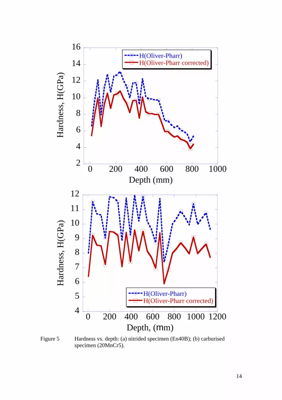
The variation of hardness as a function of depth below the surface for nitrided specimen

(En40B) and carburised specimen (20MnCr5) is shown in Figures 5a and 5b

respectively. In the nitrided specimen the hardened layer is about 0.6mm deep from the

surface and the carburised case is about 1mm. The softening near the carburised surface

(Figure 5a) is probably due to decarburisation during processing. The scatter in the

measured data is caused, in part, by the indenter encountering soft regions of retained

5

austenite. For the nitrided steel (Figure 5b) the carbonitride bands occur in the top

400m of the diffusion layer giving spikes in the hardness vs depth plot over this depth.

Below this a smoother variation in hardness is observed. The porous outer region of the

white layer causes the low hardness at the surface for the nitrided steel.

The variation of elastic modulus as a function of depth is shown in Figure 6a for

nitrided steel and in Figure 6b for carburised steel. Close to the surface very low values

for elastic modulus were recorded because the nanoindentation test has been performed

in a region where the surface influences results.

No significant differences can be observed between the values of elastic modulus of the

bulk of the specimens and case carburised and nitrided layer respectively. Zheng et al.

[10] reported much higher elastic modulus values (E=280-300GPa) for the “nitrogen

diffusion zone” compared to the Fe4N iron nitride compound layers. In the work

described in the present paper elastic modulus of the nitrided specimen do not exceeded

245GPa. Higher values reported by Zheng et al. [11] were probably affected by pile-up.

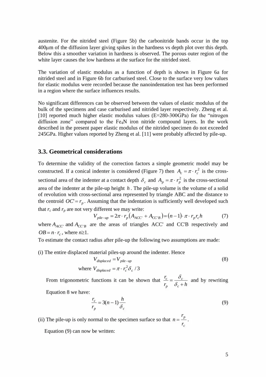
3.3. Geometrical considerations

To determine the validity of the correction factors a simple geometric model may be

constructed. If a conical indenter is considered (Figure 7) then 2cc rA is the cross-

sectional area of the indenter at a contact depth c and 2pp rA is the cross-sectional

area of the indenter at the pile-up height h . The pile-up volume is the volume of a solid

of revolution with cross-sectional area represented by triangle ABC and the distance to

the centroid prOC ' . Assuming that the indentation is sufficiently well developed such

that rc and rp are not very different we may write:

hrrnAArV cpBCCACCpuppile 12 '' (7)

where BCCACC AA '' and are the areas of triangles ACC' and CC'B respectively and

crnOB , where n1.

To estimate the contact radius after pile-up the following two assumptions are made:

(i) The entire displaced material piles-up around the indenter. Hence

uppiledisplaced VV (8)

where 3/2ccdisplaced rV

From trigonometric functions it can be shown that hr

r

c

c

p

c

and by rewriting

Equation 8 we have:

cp

c hn

r

r

)1(3 (9)

(ii) The pile-up is only normal to the specimen surface so that c

p

r

rn .

Equation (9) can now be written:

6

2

3

cp

c h

r

r

(10)

Then, from the geometry in Figure 7 and equation (8) we have:

displaceddisplacedcpp VVhhrhr 22

3

1

which gives hc 2

Equation (10) then becomes: 3/2pc rr .

From this result the correction factors can be theoretically determined:

56.0

2

'

p

c

PharrOliver

uppile

Hr

r

H

Hk (11)

75.0'

p

c

PharrOliver

uppile

Er

r

E

Ek (12)

The experimental and the theoretical approach give similar results for elastic modulus

correction factor, 75.0' EE kk . However, different results are obtained for the

hardness correction factor: 56.0 and 82.0 ' HH kk . Hardness is described by the

square of the radius ratio therefore is more sensitive to the precise radii values. Also, the

simple geometrical model does not take into account any elastic recovery of the material

and the effects of microstructure and residual stress on the geometry of the pile-up.

Finally stress concentration effects at the corners of the indenter enhance plastic

deformation and this may influence the measured area. The good agreement between

the correction factor for elastic modulus determined by this simple geometric model and

that measured is encouraging, but further work is needed to fully understand why this

approach does not work very well for hardness.

4. Conclusions

The values of hardness and elastic modulus of gear steels are overestimated by the

Oliver-Pharr analysis method due to the effect of pile-up. The slopes method diminishes

this effect but does not eliminate it. The pile-up influence on the calculation of hardness

and elastic modulus has been taken into account in this work. It can be expressed by the

mean of the correction factors PharrOliveruppileEH EEkk and HH Pharr-Oliverup-pile .

These were determined based on the contact area measured by AFM on one hand and

on a geometrical model on the other hand. The same results were obtained for elastic

modulus correction factor ( 75.0' EE kk ) but different results for the hardness

correction factor ( 82.0Hk from experimental data and 56.0' Hk from the

geometrical model). Further work is necessary to understand why there is a difference

between the calculated and measured hardness correction factors. By applying the

correction factor 75.0' EE kk to nanoindentation data accurate values for elastic

modulus were obtained. The results are in good agreement with those obtained by other

methods (e.g. conventional tensile testing) and can be reliably used in contact

mechanics calculations.

7

References

[1] G.P. Cavallaro, T.P. Wilks, C. Subramanian, K.N. Strafford, P. French, J.E. Allison,

Surf. Coat. Technol., 71 (1995) 182.

[2] P.J.L. Fernandes and C. McDuling, Eng. Failure Anal., 4 (1997) 99.

[3] W.D. Cram, In Handbook of Mechanical Wear: Wear, Frettage, Pitting, Cavitation,

Corrosion, (1961).

[4] W.C. Oliver and G.M. Pharr, J. Mater. Res., 7 (1992) 1564.

[5] I.N. Snedon, Int. J. Engng. Sci. 3 (1965) 47.

[6] J.C. Hay, A. Bolshakov, G.M. Pharr, J. Mater. Res., 14 (1999) 2296.

[7] Y. -T. Cheng and C. -M. Cheng, Surf. Coat. Technol., 133-134 (2000) 417.

[8] W.C. Oliver, J. Mater. Res. 16 (2001) 3202.

[9] S.J. Bull, Z. Metallkd., 93 (2002) 870.

[10] S.J. Bull, J.T. Evans, B.A. Shaw, D.A. Hofmann, Proc. IMechE part J: J. Eng.

Tribology, 213 (1999) 305.

[11] S. Zheng, Y. Sun, A. Bloyce, and T. Bell, Mater. Manuf. Proc. 10 (1995) 815.

8

Tables

Table 1 Chemical composition of the carburising and nitriding steels

Steel Element, weight %

C Si Mn Cr Mo V Al S P

20MnCr5 0.20 0.30 1.40 1.20 - - - <0.04 <0.025

En40B 0.27 0.27 0.47 3.05 0.43 0.08 0.03 0.019 0.024

9

Figure captions

Figure 1: Schematic diagram of the “pile-up” effect in a Berkovich

indenter/sample contact.

Figure 2 Illustration of pile-up effect around an indentation (100mN load); (a) 3D

view and (b) top view; the real area of contact is between the marking

lines.

Figure 3 (a) SEM backscattered image of EN40B nitrided steel showing the white

layer with an external porous regions and carbonitride bands in the

diffusion zone (arrowed); (b) Reflected light micrograph of 20CrMn5

carburised steel showing tempered martensite and regions of retained

austenite (arrowed).

Figure 4 (a) Hardness vs. load for EN40B steel calculated using Oliver-Pharr

method, slopes technique and Oliver-Pharr based on contact area

measured with AFM; (b) Elastic modulus vs. load for EN40B calculated

using Oliver-Pharr method, slopes technique and Oliver-Pharr based on

contact area measured with AFM.

Figure 5 Hardness vs. depth: (a) nitrided specimen (En40B); (b) carburised

specimen (20MnCr5).

Figure 6 Elastic modulus vs. depth: (a) nitrided specimen (En40B); (b) carburised

specimen (20MnCr5).

Figure 7 Pile-up around a conical indenter. It can be assumed that the volume of

displaced material equals the pile-up volume.

10

Figures

Figure 2: Schematic diagram of the “pile-up” effect in a Berkovich

indenter/sample contact.

11

Figure 2 Illustration of pile-up effect around an indentation (100mN load); (a) 3D

view and (b) top view; the real area of contact is between the marking

lines.

12

Figure 3 (a) SEM backscattered image of EN40B nitrided steel showing the white

layer with an external porous regions and carbonitride bands in the

diffusion zone (arrowed); (b) Reflected light micrograph of 20CrMn5

carburised steel showing tempered martensite and regions of retained

austenite (arrowed).

13

(a)

2.5

3

3.5

4

4.5

5

5.5

0 100 200 300 400 500 600

(a) EN40: Hardness vs. Load

H(AFM)H(Oliver-Pharr)H(slopes)

Har

dn

ess,

H(G

Pa)

Load (mN)

(b)

200

220

240

260

280

300

320

0 100 200 300 400 500 600

(b) EN40:Elastic modulus vs. Load

E(AFM)E(Oliver-Pharr)E(slopes)

Ela

stic

mo

dulu

s, E

(GP

a)

Load(mN)

Figure 4 (a) Hardness vs. load for EN40B steel calculated using Oliver-Pharr method,

slopes technique and Oliver-Pharr based on contact area measured with

AFM; (b) Elastic modulus vs. load for EN40B calculated using Oliver-

Pharr method, slopes technique and Oliver-Pharr based on contact area

measured with AFM.

14

2

4

6

8

10

12

14

16

0 200 400 600 800 1000

(a) EN40:Hardness vs. Depth

H(Oliver-Pharr)H(Oliver-Pharr corrected)

Har

dnes

s, H

(GP

a)

Depth (mm)

4

5

6

7

8

9

10

11

12

0 200 400 600 800 1000 1200

(b) 20MnCr5:Hardness vs. Depth

H(Oliver-Pharr)H(Oliver-Pharr corrected)

Har

dnes

s, H

(GP

a)

Depth, (mm)

Figure 5 Hardness vs. depth: (a) nitrided specimen (En40B); (b) carburised

specimen (20MnCr5).

15

50

100

150

200

250

300

350

0 100 200 300 400 500 600 700 800

(a) EN40:Elastic modulus vs. Depth

E(Oliver-Pharr)

E(Oliver-Pharr corrected)

Ela

stic

mo

dulu

s, E

(GP

a)

Depth, (mm)

100

150

200

250

300

350

0 200 400 600 800 1000 1200

(b) 20MnCr5:Elastic modulus vs. Depth

E(Oliver-Pharr)

E(Oliver-Pharr corrected)

Ela

stic

mo

du

lus,

E(G

Pa)

Depth (mm)

Figure 6 Elastic modulus vs. depth: (a) nitrided specimen (En40B); (b) carburised

specimen (20MnCr5).

16

Figure 7 Pile-up around a conical indenter. It can be assumed that the volume of

displaced material equals the pile-up volume.