Modeling, Analysis, Measurement and Experimentationwith the Tangram-II Integrated Environment ∗

Edmundo de S. e SilvaAna P. C. da Silva

Antonio A. de A. RochaUFRJ, COPPE/PESC, IM/CSDCxP 68511, Rio de Janeiro, RJ

21941-972, Braziledmundo@land.ufrj.br

Rosa M. M. LeaoFlavio P. Duarte

Fernando J. S. FilhoGuilherme D. G. Jaime

UFRJ, COPPE/PESCCxP 68511, RJ, Brazilrosam@land.ufrj.br

Richard R.MuntzUCLA CS Departament

Boelter Hall,Los Angeles, CA 90024, USA

muntz@cs.ucla.edu

ABSTRACTA large number of performance evaluation tools have beendeveloped over the years to support the analyst in the diffi-cult task of model building. As systems increase in complex-ity, the need is critical for tools that are able to help the userthroughout the whole modeling cycle, from model buildingto model solution and experimentation. In this work wedescribe the main features of the TANGRAM-II modelingenvironment. The tool has a powerful and flexible modelinterface, unique algorithms for the numerical solution ofmodels, includes an event driven and fluid simulators thatprovides a variety of facilities useful for obtaining the mea-sures of interest, and has a traffic engineering environmentintegrated with the other tool modules.

Categories and Subject DescriptorsC.4 [Performance of Systems]: Design studies, Measure-ment techniques, Modeling techniques, Reliability, availabil-ity, and serviceability; I.6.5 [Simulation and Modeling]:Model Development—Modeling Methodologies; I.6.8 [Simulation and Modeling]: Types of Simula-tion—Animation, Combined,Discrete event,Fluid

General TermsMeasurement,Performance,Reliability

Keywordsanalytical modeling, performance tool, simulation

1. INTRODUCTIONFor more than 30 years performance evaluation tools have

been developed to aid the modeling and analysis task. Some

∗This work is supported in part by grants from CNPq,CAPES and FAPERJ.

Permission to make digital or hard copies of all or part of this work forpersonal or classroom use is granted without fee provided that copies arenot made or distributed for profit or commercial advantage and that copiesbear this notice and the full citation on the first page. To copy otherwise, torepublish, to post on servers or to redistribute to lists, requires prior specificpermission and/or a fee.Valuetools’06 October 11-13, 2006, Pisa, ItalyCopyright 2006 ACM 01-59593-504-5 ...$5.00.

of these tools were tailored to specific applications, such asreliability/availability and queueing systems, and others al-low the specification of general models (see [12] for a surveyon the tools developed up to 1992). During these threedecades user interfaces became sophisticated and there weresignificant advances in both analytical and simulation modelsolution techniques.

The user interfaces shifted from pure textual to graphicalrepresentations of the model components, often associatedwith a high level description language. Solution techniqueshave evolved allowing very large models to be analyzed, onthe order of hundreds of thousands or millions of states.Steady state techniques benefited from the large amount ofresearch on matrix analytical techniques [48, 40, 55], bound-ing techniques [9, 47, 36, 24], Kronecker algebra [34, 49] andthose based on stochastic automata networks [53, 58]. Re-search on transient analysis advanced significantly [14], inparticular methods based on the uniformization technique[26, 18]. In parallel, new simulation techniques have beendeveloped such as those for handling rare events [30], includ-ing importance sampling and RESTART [60]. New tech-niques based on the concept of fluid flows [2, 32, 22] havealso been employed successfully to lower the computationalrequirements of computer network simulation.

Many tools have been created over the years. For instance,Petri-Net and queueing network based tools [7, 8, 29, 37, 42,20], to cite a few. With the growth of the Internet, the NSsimulation tool [33] became very popular. Furthermore, theneed for collecting measurements to understand the complexprocesses that compose Internet traffic also grew. As a con-sequence, a huge effort has been placed on the developmentof new measurement techniques capable of collecting a largevariety of statistics useful to construct models targeted totraffic engineering (e.g. [52]). Needless to say, a variety ofmeasurement tools is available.

In this paper we describe some of the features of theTANGRAM-II tool, that has been evolving for more than adecade. The main contributions of the tool are: the devel-opment of an integrated environment that includes a uniquemodeling paradigm for model especification, model solutionusing analytical solvers or simulators and, experimentationvia traffic generators and active measurement techniques;novel analytical solution methods, and techniques for fluidsimulation; new algorithms for active measurements. Theapplicability of such an environment and its modeling capa-bilities are shown through simple examples.

In section 2 we present a general overview of TANGRAM-II. Section 3 introduces its modeling environment. Section 4discusses a few analytical solvers of TANGRAM-II, as wellas the simulators implemented. Section 5 presents the trafficengineering environment. Our concluding remarks and asummary of our contributions are presented in section 6.

2. AN OVERVIEW OF TANGRAM-IIThe main purpose of a modeling tool is to provide the

necessary support to the analyst to create an abstraction ofthe system under study and to help answer questions aboutthe system behavior. First, the analyst has to estimate therange of values for the system parameters. These values canbe acquired from measurements collected from real systems,via an experimentation laboratory setup, simply “guessed”from past experience, or by comparison against similar sys-tems. Once the analyst has performed the necessary mea-surements, she can extract the parameter values from themeasurements to feed the model, for instance, to obtain thedistribution of a random variable that matches the collecteddata. The model is then constructed and solved via simula-tion or an analytical technique. The results obtained fromthe model undergo another analysis step to provide the an-swers to the questions faced by the analyst. The whole pro-cess is interactive in nature.

TANGRAM-II was built to help the analyst through themodeling steps. The tool integrates different environmentsfor developing and analyzing computer and communicationmodels. It was designed to support research, applicationdevelopment, and education in performance evaluation byproviding the ability to construct a full range of simpleto complex models and solve them by both analytical andsimulation methods. The environment includes modules toconduct active measurements in a computer network andcollect useful statistics to aid in parameterizing a model.TANGRAM-II allows the user to tailor the tool to spe-cific application domains, such as queueing, dependablity,or network modeling. Besides solution methods available inthe literature, we incorporated original techniques we devel-oped aiming at providing a rich set of options to the mod-eller. These include techniques for transient analysis, andfor solving a class of non-Markovian models [13, 4, 15]; al-gorithms for calculating measures useful for traffic analysisand experimentation [41, 19, 43] and those used for activemeasurements [56, 57]. The tool’s fluid simulator has alsodistinct features from others that allows the constructionof generic building blocks for different application domains.The same modeling paradigm is employed both for analyti-cal and simulation models and is carried through the mea-surement and experimentation modules. The tool’s moduleswere conceived to facilitate the addition of new techniquesby providing textual interfaces among modules.

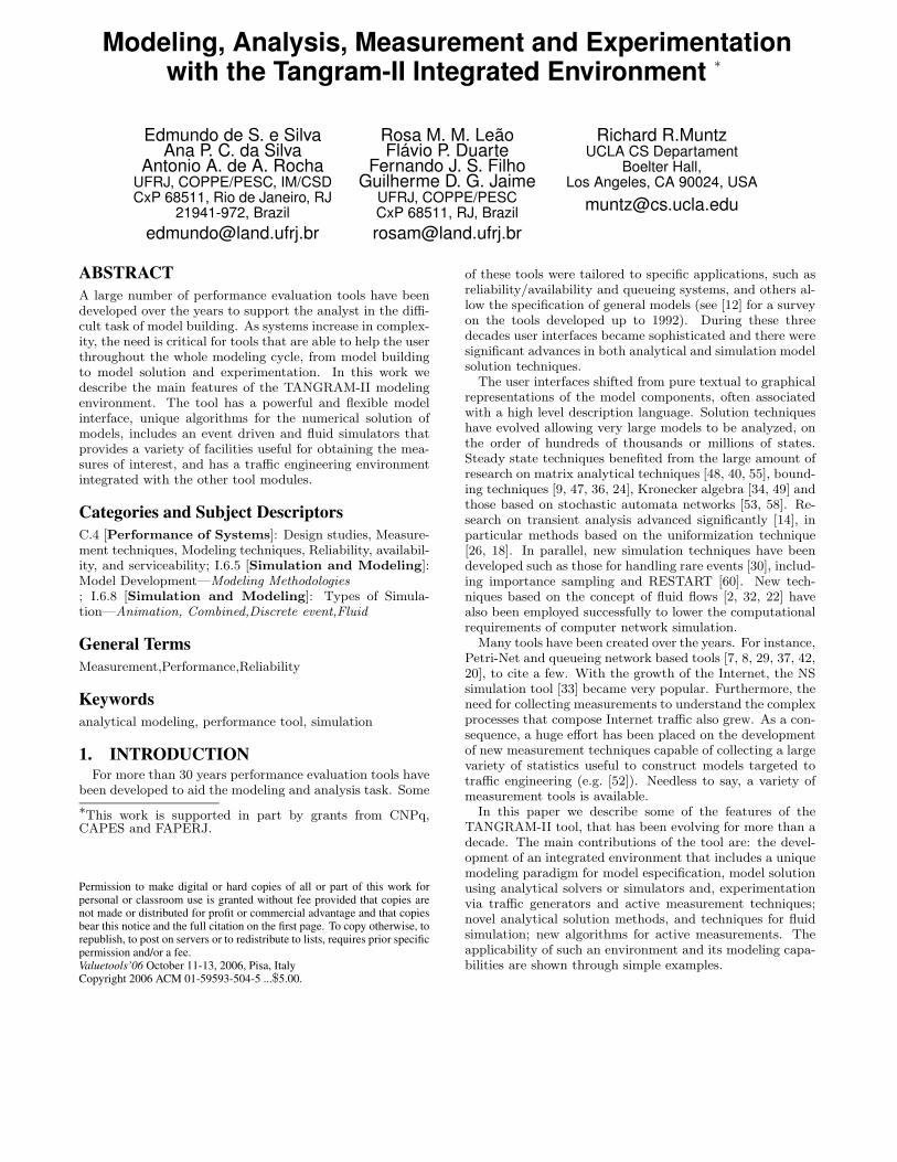
Figure 1 illustrates the main components of the TANGRAM-II environment. The top-level interface includes: (a) themodel environment; (b) the traffic engineering environmentand; (c) full fledge multimedia tools: a distributed white-board and the video/VoIP Freemeeting tool. The modelingenvironment supports the construction of simple to com-plex models, and their simulation or analytical (numerical)solution when possible. The traffic engineering environmentprovides the means to perform network measurements. Themultimedia tools are useful not only for collaborative workbut also serve as the basis for real network experimentation.

ModelingEnvironment

Whiteboard

Traffic Engineering

TrafficGeneration

steady state

transient

event driven

rare event

fluid

interactive

Simulators

animation

Voice/Videotransmission

Measuresof

Interest

marginaldistributions

conditionaldistributions

AnalyticalSolutions

support tools

activemeasurements

trafficstatistics

Figure 1: The TANGRAM-II environment.

3. THE MODELING ENVIRONMENTThe TANGRAM modeling paradigm was proposed in [3].

It was based on the observation that models are typicallymodular in that each consists of a set of objects that areconnected in some form. Each object has an internal statethat can change either due to an internally generated eventor the receipt of a message generated by another object.Events are triggered spontaneously according to a given rate(and the associated distribution) provided that a set of con-ditions specified by the user are satisfied. An object canreact to an internal event or received message by changingstate and/or sending messages to other objects.

The tool includes a library of common objects that canbe instantiated and connected to build a new model. Newobjects are developed using a template object that containsseveral attributes, such as: declarations, events, messagesand initialization. The object’s behavior is determined, fol-lowing the tool’s paradigm, from the actions that take placewhen one of the defined events occurs and how the object re-acts when a message is received. The specification of the ac-tions performed is done using a C-like language. The TAN-GRAM paradigm is quite powerful with respect to the easewith which one can specify objects with complex behavior.It allows the specification of general models and the con-struction of environments tailored to an specific applicationdomain.

Each object has a (possibly empty) set of state variableswhose values define its current state. In the TANGRAMparadigm, the overall model state is identified by the val-ues of local object states. Other types of variables can alsobe defined for an object such as parameters, and constants.The state variables can change as the result of actions as-sociated with events or a message that is received. Eventsoccur spontaneously when the associated conditions are sat-isfied. The interval between events is a random variable with

a given distribution. When an event occurs, one of a set ofactions is executed according to a given probability distri-bution. The actions can alter the current state of the objectand/or result in one or more messages being sent to otherobjects that are connected to the sender. Objects react in-stantaneously to received messages and, as a consequence,new messages can be sent to other objects, and/or the statevariables of the object may be altered.

Messages are sent to other objects via ports. Two or moreports are associated with a communication channel. Mes-sages can be broadcast to all objects connected to a channelor directed to a specific object. The sender can include datain a message that is then evaluated by the receiver.

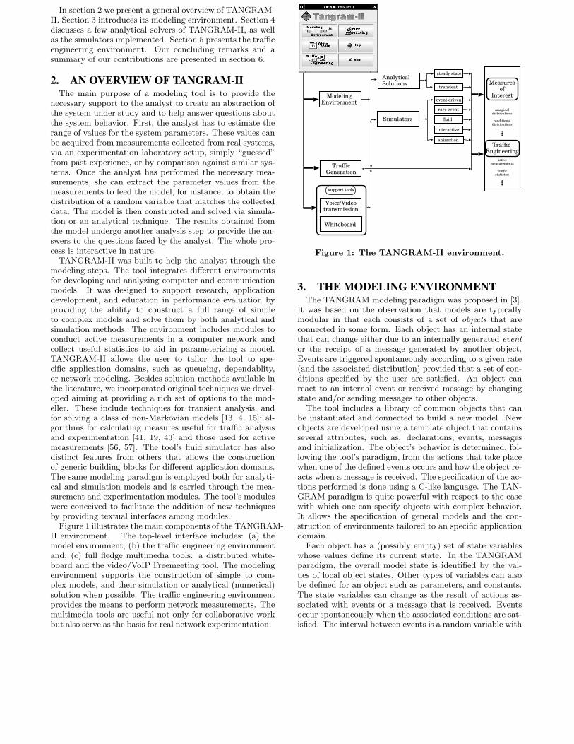
Figure 2 illustrates an example with two objects. Thefirst is an aggregate of five Markov modulated on-off sources(thus the aggregate is a birth-death model). The packetsgenerated by the sources are sent as messages to the secondobject, which represents a RED Active Queue Managementqueue, with exponentially distributed service times. REDdiscards arriving packets randomly, if the time-averaged queuelength is above a given threshold. (We used the parameterssuggested by [23].) In the model, the average queue lengthis quantized in order to obtain a discrete state space. This isan example of a Markovian model. For analytic solution themodeling environment can generate the corresponding tran-sition rate matrix in numerical or in symbolic form, accord-ing to the parameters specified. The model can be solvedanalytically or by simulation.

off on

off on

off on

...

voice_sources

Watches=ActiveSources

q

p

Watches=QueueSizeAverageQueue

RED_queue

msg_rec=PORT_INaction={ int queue_size, average_queue;

queue_size = QueueSize; average_queue = AverageQueue;

/* calculate the average queue size */ average_queue = (int)(average_queue + W_Q * (queue_size*10-average_queue));

/* set state variables */ set_st( "QueueSize", queue_size ); set_st( "AverageQueue", average_queue );} : prob = /* probability of discarding a packet */ (AverageQueue < T_MIN) * 0 + ((AverageQueue >= T_MIN) && (AverageQueue < T_MAX)) * P_MAX * (double)(AverageQueue-T_MIN) / (double) (T_MAX-T_MIN) + (AverageQueue >= T_MAX) * 1;

{ int queue_size, average_queue;

queue_size = QueueSize; average_queue = AverageQueue;

if( queue_size < BUFFER_SIZE ) queue_size++;

average_queue = (int)(average_queue + W_Q * (queue_size*10-average_queue));

/* set state variables */ set_st( "QueueSize", queue_size ); set_st( "AverageQueue", average_queue );} : prob = /* probability of not discarding a packet */ (AverageQueue < T_MIN) * 1 + ((AverageQueue >= T_MIN) && (AverageQueue < T_MAX)) * (1.0 - P_MAX * (double)(AverageQueue-T_MIN)/(double) (T_MAX-T_MIN)) + (AverageQueue >= T_MAX) * 0;

event=Service(EXP,CAPACITY)condition=( QueueSize > 0 )action={ int queue_size;

queue_size = QueueSize - 1;

set_st( "QueueSize", queue_size );};

event=Enable_Source(EXP, (NUMBER_OF_SOURCES-ActiveSources)*OFF_ON_RATE)condition=(ActiveSources < NUMBER_OF_SOURCES)action={ int active_sources;

active_sources = ActiveSources + 1;

set_st( "ActiveSources", active_sources );};

event=Disable_Source(EXP, ActiveSources*ON_OFF_RATE)condition=(ActiveSources > 0)action={ int active_sources;

active_sources = ActiveSources - 1;

set_st( "ActiveSources", active_sources );};

Figure 2: An example: model of the RED queuewith 5 sources.

From an analytical model, measures of interest can be ob-tained as functions of the state variables. Among the mea-sures of interest are: marginal distributions, distributionsof functions of state variables, conditional distributions, etc.Another way to calculate measures of interest is via the re-ward attribute.

Each object may have associated with it a reward at-tribute. TANGRAM-II allows two types of rewards to bedefined: a rate reward and an impulse reward. A rate re-ward has a given name, a set of conditions and associatedvalues. Let R be a specified reward for an object, Sc be theset of object states that satisfy condition C associated withR, and let rSC be the corresponding value assigned to R.Then, R gains rSC units of reward per time unit the objectspends in the set SC .

On the other hand, impulse rewards are associated withtransitions in the model, and are useful to count events. LetE be an event of an object, pi the probability of executingaction i when E occurs and ρE,i the impulse reward associ-ated with the reward attribute I. Then I gains ρE,i rewardunits each time action i of event E is executed. Impulse re-wards can also be associated with messages that are sent orreceived by an object.

The rewards described above are associated with an objectand so the conditions and values have their scope limitedto the set of state variables, events and messages of thatobject. However, one can also declare global rewards, andinclude the (time varying) cumulative value of the rewardsjust as any other variable in assignments to state variables,or in condition and action statements.

Rate and impulse rewards are a powerful approach to ob-tain measures of interest. One can specify complex condi-tions with rewards, and values that are constant expressions,dependent on state variables or on the cumulative values ofother rewards. The simulators also make extensive use ofthe concept of rewards and rewards are the means by whichthe modeler specifies the measures to be calculated. As willbe shown in section 4.2 reward and fluid models are tightlycoupled concepts and the fluid simulator takes full advan-tage of the reward attributes. The way by which rewards areemployed and the associated solution techniques is anothercontribution of the tool.

4. ANALYTICAL AND SIMULATION SO-LUTION TECHNIQUES

In this section we focus on a subset of the solution tech-niques available in TANGRAM-II, including transient anal-ysis methods and steady state methods that employ tran-sient analysis as part of the solution.

4.1 Analytical SolutionsAn extensive treatment of solution methods for Markov

chains can be found in [58]. MARCA is a good exam-ple of a tool that implements a rich set of steady statesolvers, from basic techniques to those appropriate for han-dling nearly completely decomposable (NCD) models andprojection methods [58]. Major advances in the numericalsolution techniques of Markov chains also include the matrixgeometric and matrix analytic methods based on the seminalwork of Neuts [48]. A tool that implements matrix-analyticalgorithms and provides solutions for continuous and dis-crete time Markov chains of QBD, GI/M/1 and M/G/1-types is MAMSolver [54].

TANGRAM-II implements a few basic iterative methodsfor solving Markov chains such as power, Gauss-Siedel andSOR. The tool’s direct method of choice is the so calledGTH algorithm [27] (and its block version) which is a sta-ble LU decomposition method for Markov chains based on

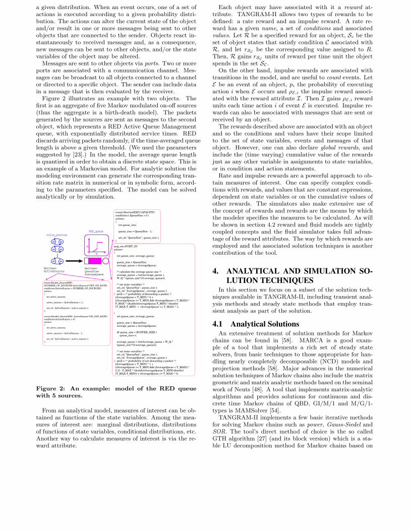
stochastic complementation [44]. This method works verywell even for large state space cardinalities. Nevertheless,other methods could be easily coupled with the tool. Figure3(a) shows the probability mass function for the RED modelof Figure 2 (with a buffer size equal to 50), when the modelis solved with GTH.

1e-04

0.001

0.01

0.1

1

0 10 20 30 40 50

Prob

abilit

y

Queue length (packets)

Queue length PMF - RED x Drop Tail

RED

Drop Tail

0 5

10 15 20 25 30 35 40 45

0 100 200 300 400 500

queu

e siz

e (re

ward

)

Time (seconds)

Sample path

(a) (b)

Figure 3: (a)PMF of the RED AQM queue using ananalytical solver; (b) queue size using reward rateand simulation.

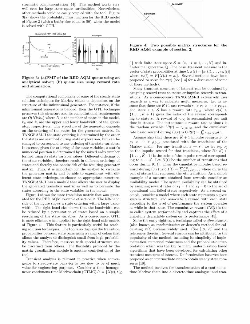
The computational complexity of some of the steady statesolution techniques for Markov chains is dependent on thestructure of the infinitesimal generator. For instance, if theinfinitesimal generator is banded, then the GTH techniquepreserves this structure and its computational requirementsare O(Nklku) where N is the number of states in the model,ku and kl are the upper and lower bandwidth of the gener-ator, respectively. The structure of the generator dependson the ordering of the states for the generator matrix. InTANGRAM-II the state ordering is determined by the orderthe states are searched during state exploration, but can bechanged to correspond to any ordering of the state variables.In essence, given the ordering of the state variables, a state’snumerical position is determined by the mixed radix numberformed using its state variable values. Different orderings ofthe state variables, therefore result in different orderings ofstates and thereby the bandwidth of the resulting generatormatrix. Thus, it is important for the analyst to visualizethe generator matrix and be able to experiment with dif-ferent state orderings, to choose an appropriate structure.TANGRAM-II has a module that allows the user to displaythe generated transition matrix as well as to permute thestates according to the state variables in the model.

Figure 4 shows the state transition matrix that was gener-ated for the RED AQM example of section 2. The left-handside of the figure shows a state ordering with a large band-width. The right-hand size shows that the bandwidth canbe reduced by a permutation of states based on a simplereordering of the state variables. As a consequence, GTHis more efficient when applied to the right-hand side matrixof Figure 4. This feature is particularly useful for teach-ing solution techniques. The tool also displays the transitionprobabilities between state pairs using a range of colors thatallows the analyst to distinguish small from high probabil-ity values. Therefore, matrices with special structure canbe discerned from others. The flexibility provided by thematrix visualization module is another contribution of thetool.

Transient analysis is relevant in practice when conver-gence to steady-state behavior is too slow to be of muchvalue for engineering purposes. Consider a time homoge-neous continuous-time Markov chain (CTMC) X = {X(t), t ≥

bandwidth

bandwidth

Figure 4: Two possible matrix structures for theRED AQM example of section 2.

0} with finite state space S = {si : i = 1, . . . , N} and in-finitesimal generator Q. One basic transient measure is thevector of state probabilities at time t, π(t) = [π1(t), . . . , πN (t)]where πi(t) = P{X(t) = si}. Several methods have beenproposed to solve for π(t) (see [14] for a discussion of someof these methods).

Many transient measures of interest can be obtained byassigning reward rates to states or impulse rewards to tran-sitions. As a consequence TANGRAM-II extensively usesrewards as a way to calculate useful measures. Let us as-sume that there areK+1 rate rewards r1 > r2 > · · · > rK+1,and state s ∈ S has a reward rate rc(s), where c(s) ∈{1, . . . , K + 1} gives the index of the reward correspond-ing to state s. A reward of rc(s) is accumulated per unittime in state s. The instantaneous reward rate at time t isthe random variable IR(t) = rc(X(t)), and the cumulative

rate based reward during (0, t) is CR(t) =R t

0rc(X(τ))dτ.

Assume also that there are bK + 1 impulse rewards ρ1 >ρ2 > · · · > ρ bK+1 associated with the transitions of the

Markov chain. For any transition s → s′, we let ρbc(s,s′)be the impulse reward for that transition, where bc(s, s′) ∈{1, . . . , bK+1} is the index of the impulse reward correspond-ing to s → s′. Let N(t) be the number of transitions thatoccur during (0, t). Then the cumulative impulse based re-

ward during (0, t) is CI(t) =PN(t)n=1 ρbc(σn) where σn is the

pair of states that represent the nth transition. As a simpleexample of a measure obtained from rewards, consider anavailability model. The system availability can be obtainedby assigning reward rates of r1 = 1 and r2 = 0 to the set ofoperational and failed states respectively. As a second ex-ample, consider a model where each state represents a givensystem structure, and associate a reward with each stateaccording to the level of performance the system operatesat while in that state. The cumulative reward CR(t) is theso called system performability and captures the effect of agracefully degradable system on its performance [45].

Since the early eighties, a technique called uniformization(also known as randomization or Jensen’s method for cal-culating π(t) became widely used. (See [18, 26] and thereferences therein). Several reasons can be attributed to thepopularity of the method, including its simplicity of imple-mentation, numerical robustness and the probabilistic inter-pretation which was the key to many uniformization basedalgorithms that have been developed for calculating othertransient measures of interest. Uniformization has even beenproposed as an intermediate step to obtain steady state mea-sures [18].

The method involves the transformation of a continuous-time Markov chain into a discrete-time analogue, and tran-

sient solutions are obtained by working with a problem indiscrete time. Consider a continuous-time Markov chain Xwith finite state space S and infinitesimal generator Q withrate from si to sj equal to qi,j , and qi =

Pj 6=i qij is the

rate out of state si. Let Λ ≥ maxi{qi}, and define the ma-trix P = I + Q/Λ. Thus P is stochastic by choice of Λ,and since Π(t) = eQt is a solution of Π′(t) = Π(t)Q, we

have: π(t) =P∞n=0 e−Λt (Λt)n

n!π(n), where π(n) = π(0)Pn.

This equation has several nice properties. It is simple, itsevaluation involves the multiplication of positive numbersonly, the error when the infinite series is truncated can beeasily bounded, the sparseness of P is preserved. One dif-ficulty was the potential overflow/underflow problem when

calculating (Λt)n

n!π(n) for large n, but a simple algorithm

exists to avoid such problem (see [12] which also points tothe original work of the authors in 1986).

Extensions to the basic approach have been proposed tosolve for models when Q changes at a finite number of timepoints or models with large Λt values. Using uniformizationone can also perform sensitivity analysis of measures basedon π(t) with respect to model parameters [31]. Furthermore,important measures from Markov reward models can be ob-tained. These include expected values such as: the expectedreward at time t, E[rX(t)]; the expected (rate) reward accu-mulated in (0, t), E[CR(t)]; the expected reward obtainedfrom transitions in (0, t), E[CI(t)]; the expected time toachieve a given reward level. Although distributions areharder to obtain than expected values, considerable progresshas been made in this area and the moments and distribu-tions of the random variables above can be calculated usinguniformization (see [18] and the references therein.)

Another class of applications for which uniformizationhas been employed is in calculating steady state measuresfor non-Markovian models. Roughly, embedded points arefound such that the behavior of the system between thesepoints is Markovian. Then the transient analysis of certainsubmodels (depending on the particular problem) are usedto calculate the transition probability matrix between theembedded points. Application examples include the analysisof: the GI/PH/1 queue [25]; schedule maintenance policiesfor computer systems [11]; polling models with timeouts [16,17]. In [15] a methodology was developed which addressesthe solution of a broad class of non-Markovian models andassociated measures. (See also [18, 14] for more details andreferences to related work.)

TANGRAM-II implements from basic to sophisticated tran-sient analysis algorithms founded on uniformization. Theseinclude a variety of reward measures (both expected valuesand distributions), as well as solutions for a class of non-Markovian models as mentioned above, and approximationtechniques (see, for instance, [13, 15, 4]).

In the next section we present the simulation capabilitiesthat TANGRAM-II offers, and specially the fluid simulator.This facility, coupled with the analytical solvers for fluidmodels, creates a powerful environment for traffic engineer-ing.

4.2 Simulation TechniquesA large variety of simulation tools are available. Perhaps

the most widely used free/open code tool is NS [33]. Theobjective of TANGRAM-II is not to implement yet anothersimulator, but to provide a simulation environment well in-tegrated with the other modules in the tool. For instance the

user can construct a Markovian model, solve it with numer-ical techniques, change the distributions of certain events,simulate the modified model and compare the results. Themodeling environment high-level interface is the same forboth the analytical solvers and the simulator. However, thesimulator includes additional high-level constructs to facil-itate the modeling task. The simulator is also integratedwith the traffic engineering environment. The user can im-port traces collected in that environment to be used as partof the simulation model. Traces can also be generated bythe simulator for the traffic engineering module.

TANGRAM-II has a large set of simulation options. Theuser is allowed to visualize the values of state variables andrewards during simulation and also alter the values of statevariables. This animation facility is a powerful teachingand debugging tool even for analytical models. Figure 3(b)shows the simulation results of a RED model (different fromthat described in Figure 2) where the queue is modeled asa fluid, using the reward rate construct.

Besides conventional simulation, TANGRAM-II implementsthe RESTART (REpetitive Simulation Trials After Reach-ing Thresholds) technique [60] to improve simulation effi-ciency when statistics of rare events are of interest. Thechoice of RESTART was due to its simplicity and efficacy.

Solving computer network models using traditional simu-lation methods could be unfeasible due to the high compu-tational cost to obtain the measures of interest when rates ofdifferent events in the model span orders of magnitude. Thisis the case, for instance, in packet simulation of high speednetworks. To mitigate this problem, a technique called fluidsimulation has been proposed [38] and can lead to a signifi-cant reduction in the computational effort.

In the fluid simulation technique, instead of representingthe individual packets in the network, the traffic is viewed asa fluid that flows through a series of reservoirs. Therefore,events associated with the arrival and departure of packetsto and from routers are not explicitly executed. Instead,only the resulting actions from changes in arrival and de-parture rates are executed and the equations that governthe changes in the fluid levels in each reservoir are solved.This can significantly reduce the time to simulate a model.

The modeling paradigm of the TANGRAM-II fluid sim-ulator is based on reward rates [10]. To our knowledge,only a few tools based on fluid simulation have been devel-oped. (See for instance, NETSIMUL [22], FluidSim [32] andreferences therein.), and both NETSIM, and FluidSim aretailored for networking modeling. TANGRAM-II, instead,implements object level constructs, that can be used to cre-ate objects tailored to different application domains.

The fluid simulator was built on top of the TANGRAM-II event driven simulator and inherited all the facilities andthe power of the TANGRAM-II tool. It is generic enoughto model complex systems and yet hides the complex fluidequations from the end user.

The paradigm used to build fluid models is based on therepresentation of the fluid reservoirs through reward rates.As such, rewards accumulate values which indicate the vol-ume of fluid in a reservoir. Objects in TANGRAM com-municate by exchanging messages. These can include anydata, for instance, a new rate for the fluid emanating fromA. As an example, suppose object A is sending a fluid toobject B at a certain rate. Also suppose a given event oc-curs at time t in A that causes a change in the flow rate

to B. Then, a message is sent from object A to B at t in-dicating that, starting from t, B will receive the fluid fromA at the new rate. Using the cumulative reward to repre-sent a reservoir in B and messages to notify rate changes,the user has available the main building blocks needed toconstruct generic fluid simulation objects and build a hy-brid fluid/conventional simulator. We know of no other toolthat have similar flexibilities.

Some network fluid objects are available in the TANGRAM-II objects library, such as traffic sources, GPS and FIFOqueues, communication links and a fluid leaky bucket. How-ever, other objects can be easily built using the featuresimplemented to support the simulation environment.

Several new constructs were developed to support the fluidsimulator paradigm and to allow the implementation of newfluid objects. The most important of them are new forms totrigger an event, in particular when specified rewards reachgiven values.

From the fluid theory, it is necessary to know when a reser-voir reaches a given threshold and triggers some action(s)to be executed when this event occurs. For example, thereservoir output fluid rate must be updated as soon as thereservoir empties. The event type called reward reached oc-curs when the specified cumulative reward reaches a certainthreshold, provided that conditions specified by the user aresatisfied. The tool automatically computes the elapsed timeuntil the occurrence of this event. This calculation is basedon the values of the instantaneous (IR(t)) and cumulativerewards (CR(t)) and the specified limit (L).

The TANGRAM-II fluid simulator also makes constructsavailable to the user to control the sum of the specified cu-mulative rewards. This is useful to model complex queuemanagement policies. For instance, to model a GPS queuewith a finite buffer fed by two or more sources, the objectqueue must keep track of the total fluid in its reservoir fromdifferent sources, as well as the individual amounts of fluidstored to compute the input and output rate.

Figure 5 shows a model example which can be built us-ing the TANGRAM-II fluid simulator. It is composed ofa router fed by two On-Off sources which are policed by aleaky bucket. The queueing discipline is GPS. A sample ofthe simulation results obtained from this model includes themean queue delay, the fraction of fluid lost and the routerutilization. Trace files can also be automatically generatedwith instantaneous and cumulative reward values. Figure6.(a) illustrates the instantaneous reward values of the leakybucket object. They represent the arrival and departure rateof the leaky bucket, the bucket state and the input queue.Figure 6.(b) shows the cumulative rewards representing the

name=sinkname=server_queue_GPSname=fluid_on_off_1name=channel_1

name=fluid_on_off_2name=channel_2

2

2

1,5

1,5

155 Mb/s

155 Mb/s

C = 155 Mb/sB = 16 MB

310 Mb/s 155 Mb/s

delay = 0,1 s

delay = 0,2 s

name=token_bucket_1

name=token_bucket_2credit_rate = 75 Mb/sbucket_size = 2 MB buffer_size = 16MB

Figure 5: GPS queue fed by two policed On-Offsources

arrivals and departures of the leaky bucket as a function oftime. We can observe the traffic shaping effect and the lowerand upper bound values of the departure rate. These plotsare very useful to evaluate the behavior of the fluids as a

function of time.

0

50

100

150

200

250

300

0 1 2 3 4 5 6 7 8

BucketBuffer

ArrivalDeparture

(a) Behavior of the leaky bucket (b) Traffic shaping

0

200

400

600

800

1000

1200

0 1 2 3 4 5 6 7 8

Arrival

Departure

Upper bound

Lower bound

Figure 6: Traces obtained from the Leaky Bucket.

5. TRAFFIC ENGINEERINGThe TANGRAM-II traffic engineering environment includes

methods for calculating measures useful for traffic model aswell as an extensive set of tools for experimentation and col-lecting parameters from the Internet. Its main features aredescribed in what follows.

5.1 Traffic ModelingTraffic characterization and modeling has been an exten-

sive area of research and a lot of work has focused on ob-taining accurate traffic models for dimensioning the networkresources. Among these models, Markovian fluid-flow mod-els (indeed rate reward models) have been widely and suc-cessfully employed. These are models for which a rewardrate is associated with each state representing, for instance,the traffic flow at a given channel. One way of parameteriz-ing the model is to match the statistics of the real trafficobserved against those from the model. For these mod-els CR(t) is the total traffic flowing through the channelin (0, t). If in turn we subtract from each reward a constantC equal to the transmission capacity of the channel, thenCR(t) is the channel queue size at t, provided that CR(t)is bounded, i.e. 0 ≤ CR(t) ≤ B where B is the maximumbuffer size.

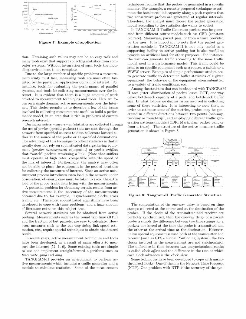
A large set of TANGRAM-II modules is dedicated to traf-fic modeling and analysis. For instance, the user has theability to create fluid-flow traffic models, obtain first andsecond order descriptors analytically or from a trace. Trafficdescriptors such as the auto-covariance function Cov(t, τ) =E[IR(t), IR(t+ τ)] − E[IR(t)]2 (for a stationary process,Cov(τ) limt→∞ Cov(t, τ)), and the index of dispersion forcounts IDC(τ) = Var[N(τ)]/E[N(τ)] for a given time lagτ (where IR(t) is the traffic rate (instantaneous reward) att and N(τ) is the process that counts the amount of traf-fic transmitted during (0, τ)). The tool uses the theory in[41] as the basis for the analytical calculations of the abovemeasures.

The user can create a performance model using the traf-fic source under study and analyze the impact of the trafficon the resources during an observation period. Figure 7(a)shows an example where the auto-covariance is plotted fortwo Markovian traffic models and from one trace, as a func-tion of the time lag. The right hand side of the figure showsthe distribution of the buffer size calculated from the fluid-flow traffic model using the technique of [19].

5.2 Measurements and experimentationThe modeling process is not complete without carefully

choosing the parameter values for the model under construc-

P[Bu

ffer(t

) > 0

.99B

]

1e-16

1e-14

1e-12

1e-10

1e-08

1e-06

0.0001

0.01

1

6000 8000 10000 12000 14000 16000 18000 20000

load = 0.9

load = 0.6

Buffer size

t = 10s

-5e+06

0

5e+06

1e+07

1.5e+07

2e+07

2.5e+07

3e+07

3.5e+07

4e+07

0 0.02 0.04 0.06 0.08 0.1 0.12 0.14 0.16

trace

Pseudo self-similar model

MMPP model

(t) time lag (sec)

Cov(

t)

(a) Auto-covariance (a) Buffer size distribution

Figure 7: Example of application

tion. Obtaining such values may not be an easy task andmany tools exist that support collecting statistics from com-puter systems. Without integration of such tools the mod-eling environment is not complete.

Due to the large number of specific problems a measure-ment study must face, measuring tools are most often tar-geted to the particular application domain of interest. Forinstance, tools for evaluating the performance of parallelsystems, and tools for collecting measurements over the In-ternet. It is evident that there is a huge amount of workdevoted to measurement techniques and tools. Here we fo-cus on a single domain: active measurements over the Inter-net. This choice permits us to describe a few of the issuesinvolved in collecting measurements useful to build a perfor-mance model, in an area that is rich in problems of currentresearch interest.

During an active measurement statistics are collected throughthe use of probes (special packets) that are sent through thenetwork from specified sources to data collectors located ei-ther at the source of the probe or at specified destinations.The advantage of this technique to collect statistics is that itusually does not rely on sophisticated data gathering equip-ment (passive measurement equipment) or packet sniffersthat “watch” packets traversing a link. (Note that sniffersmust operate at high rates, compatible with the speed ofthe link of interest.) Furthermore, the analyst may oftennot be able to place the equipment in the needed locationsfor collecting the measures of interest. Since an active mea-surement process introduces extra load in the network underobservation, obviously care must be taken to avoid the extraload of the probe traffic interfering with the measurements.

A potential problem for obtaining certain results from ac-tive measurements is the inaccuracy of the measurementsobtained due to, for example, unsynchronized clocks, crosstraffic, etc. Therefore, sophisticated algorithms have beendeveloped to cope with these problems, and a huge amountof literature exists on this subject area.

Several network statistics can be obtained from activeprobing. Measurements such as the round trip time (RTT)and the fraction of lost packets, are easy to calculate. How-ever, measures such as the one-way delay, link speed esti-mation, etc., require special techniques to obtain the desiredresult.

In recent years, active measurement techniques and toolshave been developed, as a result of many efforts to mea-sure the Internet [52, 1, 6]. Some existing tools are simpleto use and implement straightforward algorithms such astraceroute, ping and bing.

TANGRAM-II provides an environment to perform ac-tive measurements which includes a traffic generator and amodule to calculate statistics. Some of the measurement

techniques require that the probes be generated in a specificmanner. For example, a recently proposed technique to esti-mate the bottleneck link capacity along a path requires thattwo consecutive probes are generated at regular intervals.Therefore, the analyst must choose the packet generationmodel according to the statistics she wants to collect.

In TANGRAM-II Traffic Generator packets can be gener-ated from different source models such as: CBR (constantbit rate), Markovian, packet pair, or from a trace providedby the user. It is important to note that the packet gen-eration module in TANGRAM-II is not only useful as asupporting facility to active probing but is also useful toprovide an artificial load for other purposes. For instance,the user can generate traffic according to the same trafficmodel used in a performance model. This traffic could besend to an specific equipment such as a router, a switch or aWWW server. Examples of simple performance studies are:to generate traffic to determine buffer statistics of a givenequipment, the behavior of the equipment when submittedto a variety of traffic conditions, etc.

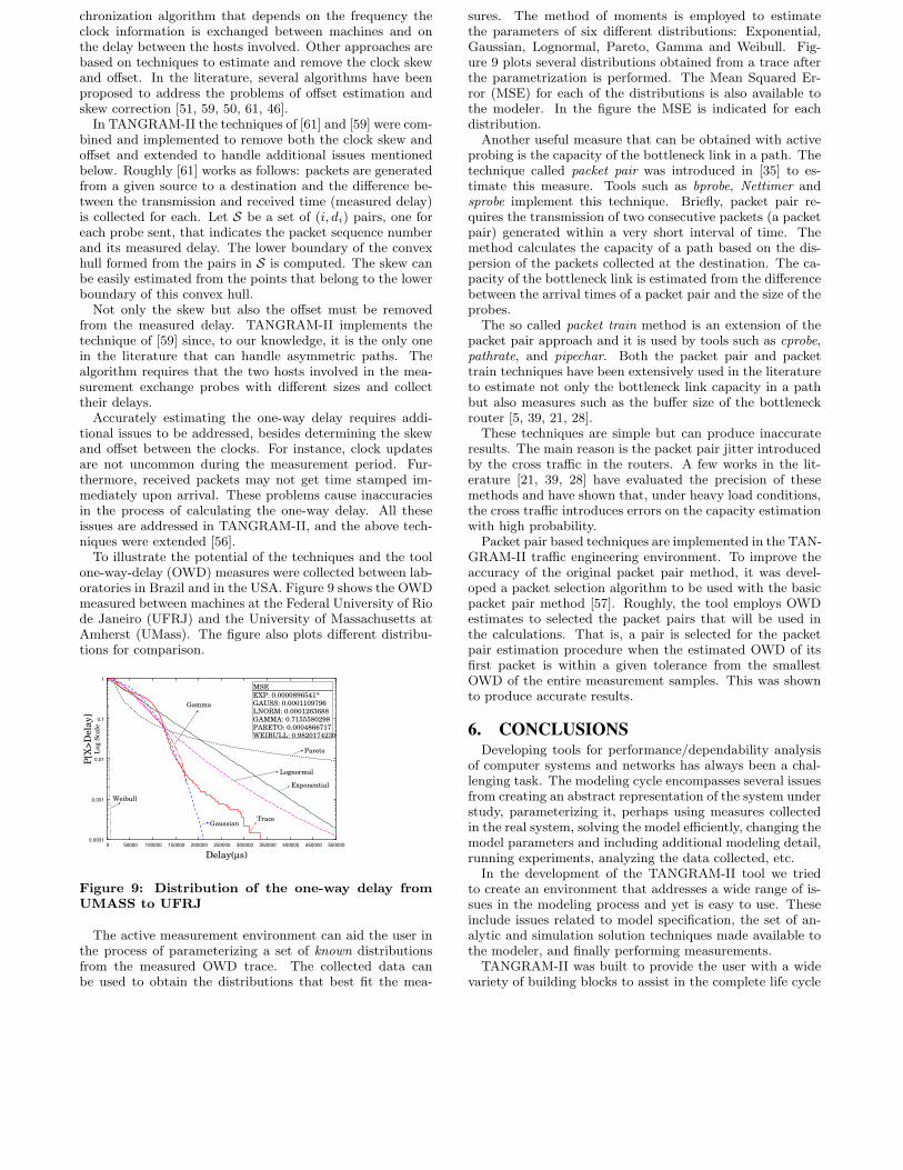
Among the statistics that can be obtained with TANGRAM-II are: jitter, distribution of packet losses, RTT, one-waydelay, bottleneck capacity of a path, and bottleneck buffersize. In what follows we discuss issues involved in collectingsome of these statistics. It is interesting to note that, inorder to estimate some of the metrics, probes may be gen-erated in different directions between two points (one-way,two-way or round-trip), and employing different traffic gen-eration patterns/models (CBR, Markovian, packet pair, orfrom a trace). The structure of the active measure trafficgeneration is shown in Figure 8.

TANGRAM-IITraffic Generator

SET-1One-way Measures

SET-2Two One-way Measures

SET-3Round Trip Measures

CBR Markov Trace CBR PacketPair

CBR Markov Trace PacketPair

Probes GenerationDirection

Probes GenerationModel

* 1-way Delay* Jitter* Loss* Consecutive Loss* Success* Throughput

* 1-way Delay* Bottleneck Capacity* Buffer Size

* RTT* Jitter* Loss* Consecutive Loss* Success* Throughput

* RTT* Loss* Consecutive Loss* Success* Throughput

* RTT* Loss* Consecutive Loss* Success* Throughput

* RTT* Bottleneck Capacity* Buffer Size

* Jitter* Loss* Consecutive Loss* Success* Throughput

* Loss* Consecutive Loss* Success* Throughput

* Loss* Consecutive Loss* Success* Throughput

Figure 8: Tangram-II Traffic Generator Structure.

The computation of the one-way delay is based on timestamps collected at the source and at the destination of theprobes. If the clocks of the transmitter and receiver areperfectly synchronized, then the one-way delay of a packetprobe is simply the difference between two time stamps for apacket: one issued at the time the probe is transmitted andthe other at the arrival time at the destination. However,unless special equipment is used both at the transmitter andreceiver (such as GPS - Global Positioning System), the twoclocks involved in the measurement are not synchronized.The difference in time between two unsynchronized clocksis called clock offset and the difference in the rate at whicheach clock advances is the clock skew.

Some techniques have been developed to cope with unsyn-chronized clocks. One of them is the Network Time Protocol(NTP). One problem with NTP is the accuracy of the syn-

chronization algorithm that depends on the frequency theclock information is exchanged between machines and onthe delay between the hosts involved. Other approaches arebased on techniques to estimate and remove the clock skewand offset. In the literature, several algorithms have beenproposed to address the problems of offset estimation andskew correction [51, 59, 50, 61, 46].

In TANGRAM-II the techniques of [61] and [59] were com-bined and implemented to remove both the clock skew andoffset and extended to handle additional issues mentionedbelow. Roughly [61] works as follows: packets are generatedfrom a given source to a destination and the difference be-tween the transmission and received time (measured delay)is collected for each. Let S be a set of (i, di) pairs, one foreach probe sent, that indicates the packet sequence numberand its measured delay. The lower boundary of the convexhull formed from the pairs in S is computed. The skew canbe easily estimated from the points that belong to the lowerboundary of this convex hull.

Not only the skew but also the offset must be removedfrom the measured delay. TANGRAM-II implements thetechnique of [59] since, to our knowledge, it is the only onein the literature that can handle asymmetric paths. Thealgorithm requires that the two hosts involved in the mea-surement exchange probes with different sizes and collecttheir delays.

Accurately estimating the one-way delay requires addi-tional issues to be addressed, besides determining the skewand offset between the clocks. For instance, clock updatesare not uncommon during the measurement period. Fur-thermore, received packets may not get time stamped im-mediately upon arrival. These problems cause inaccuraciesin the process of calculating the one-way delay. All theseissues are addressed in TANGRAM-II, and the above tech-niques were extended [56].

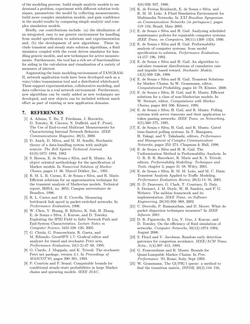
To illustrate the potential of the techniques and the toolone-way-delay (OWD) measures were collected between lab-oratories in Brazil and in the USA. Figure 9 shows the OWDmeasured between machines at the Federal University of Riode Janeiro (UFRJ) and the University of Massachusetts atAmherst (UMass). The figure also plots different distribu-tions for comparison.

Delay(µs)

P[X>

Del

ay]

Log

Scal

e

0.0001

0.001

0.01

0.1

1

0 50000 100000 150000 200000 250000 300000 350000 400000 450000 500000

Weibull

Gaussian Trace

Lognormal

Pareto

Exponential

Gamma

MSEEXP: 0.0000896541*GAUSS: 0.0001109796LNORM: 0.0001263688GAMMA: 0.7155580298PARETO: 0.0004866717WEIBULL: 0.9820174230

Figure 9: Distribution of the one-way delay fromUMASS to UFRJ

The active measurement environment can aid the user inthe process of parameterizing a set of known distributionsfrom the measured OWD trace. The collected data canbe used to obtain the distributions that best fit the mea-

sures. The method of moments is employed to estimatethe parameters of six different distributions: Exponential,Gaussian, Lognormal, Pareto, Gamma and Weibull. Fig-ure 9 plots several distributions obtained from a trace afterthe parametrization is performed. The Mean Squared Er-ror (MSE) for each of the distributions is also available tothe modeler. In the figure the MSE is indicated for eachdistribution.

Another useful measure that can be obtained with activeprobing is the capacity of the bottleneck link in a path. Thetechnique called packet pair was introduced in [35] to es-timate this measure. Tools such as bprobe, Nettimer andsprobe implement this technique. Briefly, packet pair re-quires the transmission of two consecutive packets (a packetpair) generated within a very short interval of time. Themethod calculates the capacity of a path based on the dis-persion of the packets collected at the destination. The ca-pacity of the bottleneck link is estimated from the differencebetween the arrival times of a packet pair and the size of theprobes.

The so called packet train method is an extension of thepacket pair approach and it is used by tools such as cprobe,pathrate, and pipechar. Both the packet pair and packettrain techniques have been extensively used in the literatureto estimate not only the bottleneck link capacity in a pathbut also measures such as the buffer size of the bottleneckrouter [5, 39, 21, 28].

These techniques are simple but can produce inaccurateresults. The main reason is the packet pair jitter introducedby the cross traffic in the routers. A few works in the lit-erature [21, 39, 28] have evaluated the precision of thesemethods and have shown that, under heavy load conditions,the cross traffic introduces errors on the capacity estimationwith high probability.

Packet pair based techniques are implemented in the TAN-GRAM-II traffic engineering environment. To improve theaccuracy of the original packet pair method, it was devel-oped a packet selection algorithm to be used with the basicpacket pair method [57]. Roughly, the tool employs OWDestimates to selected the packet pairs that will be used inthe calculations. That is, a pair is selected for the packetpair estimation procedure when the estimated OWD of itsfirst packet is within a given tolerance from the smallestOWD of the entire measurement samples. This was shownto produce accurate results.

6. CONCLUSIONSDeveloping tools for performance/dependability analysis

of computer systems and networks has always been a chal-lenging task. The modeling cycle encompasses several issuesfrom creating an abstract representation of the system understudy, parameterizing it, perhaps using measures collectedin the real system, solving the model efficiently, changing themodel parameters and including additional modeling detail,running experiments, analyzing the data collected, etc.

In the development of the TANGRAM-II tool we triedto create an environment that addresses a wide range of is-sues in the modeling process and yet is easy to use. Theseinclude issues related to model specification, the set of an-alytic and simulation solution techniques made available tothe modeler, and finally performing measurements.

TANGRAM-II was built to provide the user with a widevariety of building blocks to assist in the complete life cycle

of the modeling process: build simple analytic models to un-derstand a problem, experiment with different solution tech-niques, parametrize the model by collecting measurements,build more complex simulation models, and gain confidencein the model results by comparing simple analytic and com-plex simulation models.

Briefly, our contributions include: (a) the idealization ofan integrated, easy to use generic environment for handlingfrom model specification to solutions and experimentationand; (b) the development of new algorithms. These in-clude transient and steady state solution algorithms, a fluidsimulator coupled with the event driven simulator for han-dling generic models, and new techniques for active measure-ments. Furthermore, the tool has a rich set of functionalitiesfor aiding in the calculation and visualization of a variety ofmeasures of interest.

Augmenting the basic modeling environment of TANGRAM-II, network application tools have been developed such as avoice/video transmission tool and a distributed whiteboard.These support experimentation, collaborative modeling, anddata collection in a real network environment. Furthermore,new algorithms can be easily added as new techniques aredeveloped, and new objects can be included without mucheffort as part of existing or new application domains.

7. REFERENCES[1] A. Adams, T. Bu, T. Friedman, J. Horowitz,

D. Towsley, R. Caceres, N. Duffield, and F. Presti.The Use of End-to-end Multicast Measurements forCharacterizing Internal Network Behavior. IEEECommunications Magazine, 38(5), 2000.

[2] D. Anick, D. Mitra, and M. M. Sondhi. Stochastictheory of a data-handling system with multiplesources. The Bell System Technical Journal,61(8):1871–1894, 1982.

[3] S. Berson, E. de Souza e Silva, and R. Muntz. Anobject oriented methodology for the specification ofMarkov models. In Numerical Solution of MarkovChains, pages 11–36. Marcel Dekker, Inc., 1991.

[4] R. M. L. R. Carmo, E. de Souza e Silva, and R. Marie.Efficient solutions for an approximation technique forthe transient analysis of Markovian models. Technicalreport, IRISA, no. 3055, Campus universitaire deBeaulieu, 1996.

[5] R. L. Carter and M. E. Crovella. Measuringbottleneck link speed in packet-switched networks. InPerformance Evaluation, 1996.

[6] W. Chen, Y. Huang, B. Ribeiro, K. Suh, H. Zhang,E. de Souza e Silva, J. Kurose, and D. Towsley.Exploiting the IPID Field to Infer Network Path andEnd-System Characteristics. Lecture Notes inComputer Science, 3431:108–120, 2005.

[7] G. Chiola, G. Franceschinis, R. Gaeta, andM. Ribaudo. GreatSPN 1.7: Grafical editor andanalyzer for timed and stochastic Petri nets.Performance Evaluation, 24(1-2):47–68, 1995.

[8] G. Ciardo, J. Muppala, and K. Trivedi. The stochasticPetri net package, version 3.1. In Proceedings ofMASCOT’93, pages 390–391, 1993.

[9] P. Courtois and P. Semal. Computable bounds forconditional steady-state probabilities in large Markovchains and queueing models. IEEE JSAC,

4(6):926–937, 1986.

[10] K. de Freitas Reinhardt, E. de Souza e Silva, andR. M. M. Leao. A Fluid Simulation Environment forMultimedia Networks. In XXI Brazilian Symposiumon Communication Networks (in portuguese), pages119–134, Brazil, Maio 2003.

[11] E. de Souza e Silva and H. Gail. Analyzing scheduledmaintenance policies for repairable computer systems.IEEE Trans. on Computers, 39(11):1309–1324, 1990.

[12] E. de Souza e Silva and H. Gail. Performabilityanalysis of computer systems: from modelspecification to solution. Performance Evaluation,14:157–196, 1992.

[13] E. de Souza e Silva and H. Gail. An algorithm tocalculate transient distributions of cumulative rateand impulse based reward. Stochastic Models,14(3):509–536, 1998.

[14] E. de Souza e Silva and H. Gail. Transient Solutionsfor Markov Chains. In W. Grassmann, editor,Computational Probability, pages 44–79. Kluwer, 2000.

[15] E. de Souza e Silva, H. Gail, and R. Muntz. Efficientsolutions for a class of non-Markovian models. InW. Stewart, editor, Computations with MarkovChains, pages 483–506. Kluwer, 1995.

[16] E. de Souza e Silva, H. Gail, and R. Muntz. Pollingsystems with server timeouts and their application totoken passing networks. IEEE Trans. on Networking,3(5):560–575, 1995.

[17] E. de Souza e Silva, H. Gail, and R. Muntz. Gatedtime-limited polling systems. In T. Hasegawa,H. Takagi, and Y. Takahashi, editors, Performanceand Management of Complex CommunicationNetworks, pages 253–274. Chapman & Hall, 1998.

[18] E. de Souza e Silva and H. R. Gail. TheUniformization Method in Performability Analysis. InG. R. B. R. Haverkort, R. Marie and K. S. Trivedi,editors, Performability Modelling: Techniques andTools, chapter 3, pages 31–58. Wiley, 2001.

[19] E. de Souza e Silva, R. M. M. Leao, and M. C. Diniz.Transient Analysis Applied to Traffic Modeling.Performance Evaluation Review, 28(4):14–16, 2001.

[20] D. D. Deavours, G. Clark, T. Courtney, D. Daly,S. Derisavi, J. M. Doyle, W. H. Sanders, and P. G.Webster. The mobius framework and itsimplementation. IEEE Trans. on SoftwareEngineering, 28(10):956–969, 2002.

[21] C. Dovrolis, P. Ramanathan, and D. Moore. What dopacket dispersion techniques measures? In IEEEInfocom 2001.

[22] D. R. Figueiredo, B. Liu, Y. Guo, J. Kurose, andD. Towsley. On the efficiency of fluid simulation ofnetworks. Computer Networks, 50(12):1974–1994,August 2006.

[23] S. Floyd and V. Jacobson. Random early detectiongateways for congestion avoidance. IEEE/ACM Trans.Netw., 1(4):397–413, 1993.

[24] G. Franceschinis and R. Muntz. Bounds forQuasi-Lumpable Markov Chains. In Proc.Performance ’93, Rome, Italy, Sept 1993.

[25] W. Grassmann. The GI/PH/1 queue: a method tofind the transition matrix. INFOR, 20(2):144–156,

1982.

[26] W. Grassmann. Finding transient solutions inMarkovian event systems through randomization. InW. J. Stewart, editor, Numerical Solution of MarkovChains, pages 357–371. Marcel Dekker, Inc., 1991.

[27] W. Grassmann, M. Taksar, and D. Heyman.Regenerative analysis and steady state distributionsfor Markov chains. Operations Research,33(5):1107–1116, 85.

[28] K. Harfoush, A. Bestravos, and J. Byers. Measuringbottleneck bandwidth of targeted path segments. InIEEE Infocom 2003.

[29] B. Haverkort. Performability evaluation offault-tolerant computer systems using DyQNtool+.Int’l Journal Reliability, Quality and Safety Eng.,2(4):383–404, 1995.

[30] P. Heidelberger. Fast simulation of rare events inqueueing and reliability models. ACM Transactions onModeling and Computer Simulation, 5(1):43–85, 1995.

[31] P. Heidelberger and A. Goyal. Sensitivity analysis ofcontinuous time Markov chains using uniformization.In G. Iazeolla, P. Courtois, and O. Boxma, editors,Computer Performance and Reliability, pages 93–104.North-Holland, 1988.

[32] J. Incera, R. Marie, D. Ross, and G. Rubino.FluidSim: A Tool to Simulate Fluid Models of HighSpeed Networks. Performance Evaluation, 44:25–49,2001.

[33] Insecure.org. Network Simulator.http://www.isi.edu/nsnam/ns.

[34] K. Irani and V.L.Wallace. On network linguistics andthe conversational design of queueing networks.Journal of the ACM, 18:616–629, 1971.

[35] V. Jacobson. Congestion avoidance and control. InACM SIGCOMM 1988, pages 314–329.

[36] J.C.S. Lui and R.R. Muntz. Bounding Methodologyfor Computing Steady State Availability of RepairableComputer Systems. Journal of the ACM,41(4):676–707, 1994.

[37] R. L. Klevans and W. J. Stewart. From queueingnetworks to markov chains: The XMARCA interface.Performance Evaluation, 24(1-2):23–45, 1995.

[38] K. Kumaram and D. Mitra. Performance and FluidSimulations of a Novel Shared Buffer ManagementSystem. In IEEE Infocom 1998.

[39] K. Lai and M. Baker. Measuring bandwidth. In IEEEInfocom 1999.

[40] G. Latouche. Algorithms for Infinite Markov chainswith Repeating Columns. In Linear Algebra, MarkovChains, and Queueing Models, pages 231–266. 1993.

[41] R. M. M. Leao, E. de Souza e Silva, and S. C.de Lucena. A Set of Tools for Traffic Modeling,Analysis and Experimentation. In Lecture Notes inComputer Science, volume 1786, pages 40–55.Springer, March 2000.

[42] C. Lindemann. DSPNexpress: A software package forthe efficient solution of deterministic and stochasticpetri nets. Performance Evaluation, 22(1):3–21, 1995.

[43] M. Martinello and E. de Souza e Silva. A testbed fornetwork performance evaluation and its application toconnection admission control algorithms. Journal of

the Brazilian Computer Society, 7(2):39–51, 2001.

[44] C. Meyer. Stochastic complementation, uncouplingMarkov chains, and the theory of nearly reduciblesystems. SIAM Review, 31(2):240–272, 1989.

[45] J. Meyer. On evaluating the performability ofdegradable computing systems. IEEE Trans. onComputers, C-29(8):720–731, 1980.

[46] S. B. Moon, P. Skelly, and D. Towsley. Estimation andremoval of clock skew for network delaymeasurements. In IEEE Infocom 1999.

[47] R. Muntz, E. de Souza e Silva, and A. Goyal.Bounding availability of repairable computer systems.IEEE Trans. on Computers, 38(12):1714–1723, 1989.

[48] M. F. Neuts. Matrix-geometric Solutions in StochasticModels – an Algorithmic Approach. John HopkinsUniversity Press, Baltimore, MD, 1981.

[49] P. Buchholz and G. Ciardo and S. Donatelli and P.Kemper. Kronecker Operations and Sparse Matriceswith Applications to the Solution of Markov Models.INFORMS Journal on Computing, 12(3):203–222,2000.

[50] A. Pasztor and D. Veitch. PC Based Precision TimingWithout GPS. In ACM Sigmetrics 2002.

[51] V. Paxson. On calibrating measurements of packettransit times. In ACM Sigmetrics 1998.

[52] V. Paxson, A. Adams, and M. Mathis. Experienceswith NIMI. In Proc. of Passive and ActiveMeasurement, 2000.

[53] B. Plateau. On the stochastic structure of parallelismand synchronization models for distributedalgorithms. In ACM Sigmetrics 1985.

[54] A. Riska and E. Smirni. MAMSolver: a MatrixAnalytic Methods Tool. In Lecture Notes in ComputerScience, volume 2324, pages 205–211. Springer, 2002.

[55] A. Riska and E. Smirni. M/G/1-Type MarkovProcesses: A Tutorial. In Performance Evaluation ofComplex Systems: Techniques and Tools, volume 2459of LNCS, pages 36–63. 2002.

[56] A. A. A. Rocha, R. M. M. Leao, and E. de Souza eSilva. A Methodology to Estimate One-way Delay andInternet Experiments (in portuguese). In XXIIBrazilian Computer Network Symposium(SBRC’04),Gramado, Brazil, May 2004.

[57] A. A. A. Rocha, R. M. M. Leao, and E. de Souza eSilva. A New Technique to Select Packet Pairs toEstimate Bottleneck Link Capacity (in portuguese). InIII WPerformance/XXIV SBC, Salvador, Brazil,August 2004.

[58] W. Stewart. Introduction to the Numerical Solution ofMarkov Chains. Princeton University Press, 1994.

[59] M. Tsuru, T. Takine, and Y. Oie. Estimation of clockoffset from one-way delay measurement on asymmetricpaths. In SAINT International Symposium onApplications and the Internet, 2002.

[60] M. Villen-Altamirano and J. Villen-Altamirano.RESTART: A Straightforward Method for FastSimulation of Rare Events. In Proceedings of the 1994Winter Simulation Conference, pages 282–289.

[61] L. Zhang, Z. Liu, and C. H. Xia. Clocksynchronization algorithms for network measurements.In IEEE Infocom 2002.