Seediscussions,stats,andauthorprofilesforthispublicationat:https://www.researchgate.net/publication/262685945

EMLab-Generation-Anexperimentationenvironmentforelectricitypolicyanalysis

TECHNICALREPORT·JANUARY2013

CITATION

1

READS

42

3AUTHORS,INCLUDING:

L.J.DeVries

DelftUniversityofTechnology

69PUBLICATIONS403CITATIONS

SEEPROFILE

EmileChappin

DelftUniversityofTechnology

94PUBLICATIONS239CITATIONS

SEEPROFILE

Availablefrom:EmileChappin

Retrievedon:04February2016

EMLab-GenerationAn experimentation environment for electricity policy analysis

Version 1.0, February, 2013

Laurens J. de Vries, Émile J. L. Chappin and Jörn C. Richstein

More information: http://emlab.tudelft.nl/generation

Please refer to this report as: De Vries, L.J., E.J.L. Chappin & J.C. Richstein, EMLab-Generation – Anexperimentation environment for electricity policy analysis, TU Delft, 2013.

Copyright c© 2013 by TU Delft

Contents

List of Figures v

List of Tables vii

1 Introduction 1

2 Description of the Agent-Based Model 32.1 Overview . . . . . . . . . . . . . . . . . . . . . . . . . . . . . . . . . . . . . . . . 32.2 Agents . . . . . . . . . . . . . . . . . . . . . . . . . . . . . . . . . . . . . . . . . 42.3 Generation technologies . . . . . . . . . . . . . . . . . . . . . . . . . . . . . . . 62.4 Intermittent energy sources . . . . . . . . . . . . . . . . . . . . . . . . . . . . . 72.5 Power plant operation and spot market bidding . . . . . . . . . . . . . . . . . 72.6 The electricity and CO2 market algorithms . . . . . . . . . . . . . . . . . . . . 72.7 Investment algorithm . . . . . . . . . . . . . . . . . . . . . . . . . . . . . . . . . 112.8 Exogenous scenarios . . . . . . . . . . . . . . . . . . . . . . . . . . . . . . . . . 14

3 Implementation in AgentSpring 153.1 AgentSpring framework . . . . . . . . . . . . . . . . . . . . . . . . . . . . . . . 153.2 User interface . . . . . . . . . . . . . . . . . . . . . . . . . . . . . . . . . . . . . 153.3 The system captured in a database . . . . . . . . . . . . . . . . . . . . . . . . . 163.4 Types of classes and other files . . . . . . . . . . . . . . . . . . . . . . . . . . . 173.5 Modelling agents and their behavior . . . . . . . . . . . . . . . . . . . . . . . . 183.6 Development and documentation . . . . . . . . . . . . . . . . . . . . . . . . . . 18

Appendices 21

A Power plant and fuel data 23A.1 Energy densities of fuels . . . . . . . . . . . . . . . . . . . . . . . . . . . . . . . 23A.2 Power plant data . . . . . . . . . . . . . . . . . . . . . . . . . . . . . . . . . . . 23

B Sample load-duration function 25

Acknowledgements 27

Bibliography 29

iii

Contents

iv

List of Figures

2.1 Structure of the model . . . . . . . . . . . . . . . . . . . . . . . . . . . . . . . . . . 52.2 Structure of the market clearing algorithm . . . . . . . . . . . . . . . . . . . . . . . 82.3 Structure of the investment algorithm . . . . . . . . . . . . . . . . . . . . . . . . . 12

3.1 Snapshot of the user interface of AgentSpring with the model running . . . . . . 163.2 The graph of possible relations for an electricity spot market . . . . . . . . . . . . 173.3 Snapshot of the documentation of the model as a website . . . . . . . . . . . . . . 19

B.1 Sample load-duration curve . . . . . . . . . . . . . . . . . . . . . . . . . . . . . . . 26

v

List of Figures

vi

List of Tables

2.1 Notation . . . . . . . . . . . . . . . . . . . . . . . . . . . . . . . . . . . . . . . . . . 102.2 Fuel price scenario . . . . . . . . . . . . . . . . . . . . . . . . . . . . . . . . . . . . 14

A.1 Conversion factors for power plants . . . . . . . . . . . . . . . . . . . . . . . . . . 23A.2 Power plant data . . . . . . . . . . . . . . . . . . . . . . . . . . . . . . . . . . . . . 24

B.1 Sample load-duration function . . . . . . . . . . . . . . . . . . . . . . . . . . . . . 25

vii

List of Tables

viii

1 Introduction

There is a growing consensus that Europe’s electricity sector must be nearly or completely Transforming theelectricity sectorcarbon-free by the middle of this century. This will need to be achieved with a combination

of a substantial amount of renewable energy and perhaps nuclear power and/or the use offossil fuels with carbon capture and sequestration. The current approach is to regulate CO2emissions through the EU-ETS and provide additional stimulus for renewable energy. Thelatter policy is implemented at the national level, as a result of which there is considerableheterogeneity in these policies (although there appears to be a tendency towards feed-intariffs). In addition, countries have specific policies regarding the use of nuclear fuels,the combustion of coal and carbon capture and sequestration. The resulting variety ofelectricity market policies is further compounded by differences in basic electricity marketdesign, for instance with respect to transmission regulation, congestion management andthe balancing mechanism.

The central question in this research is what the combined effect is of different policy Understanding complexmarket behaviorinstruments (in particular carbon policy and renewable energy policy) upon an electricity

market, in isolation and in combination with neighboring electricity markets with differentpolicies, are. What happens when two interconnected electricity markets, both participat-ing in the EU-ETS, have different renewable energy policies? What if one of these decidesto phase out nuclear power? What would be the effect of a minimum price for CO2? Whatif this were implemented in only one country?

While the EU-ETS is an effective instrument for allocating CO2 emission reductions EU-ETS

among large producers in Europe, it has failed to trigger the kinds of long-range invest-ments that will be necessary for achieving substantial emissions reductions in the future.Two reasons can be given for this failure. The first is that the ETS does not provide a strongenough investment incentive, in part because the average CO2 price is too low, and in partbecause the CO2 price is too volatile. The second reason is that investment decisions arealso affected by carbon and renewable energy policy, the design of the electricity market(especially a capacity mechanism may have a strong impact), availability of locations fornew plant, permit restrictions etcetera.

A second issue of concern is the phenomenon that electricity prices can be expected to Electricity prices

become more volatile as low-carbon electricity generation technologies gain market share,because their marginal costs of generation tend to be relatively low. As a result, electricityprices can be expected to be below average cost during periods with ample generation ca-pacity, which means that peak prices will need to be higher for power companies to recovertheir costs. This higher volatility is likely to discourage investment in capital-intensivetechnologies, slowing down the desired investment in many low-carbon technologies.

To address these issues, a dynamic simulation model will be developed. Equilibrium Research approach

models do not capture the intertemporal relations (which exist due to path dependence)that affect the long-term development of the electricity sector. This model will need to besuitable for incorporating multiple policy instruments and multiple, connected electricitymarkets. Finally, the model will need to include a rich representation of investment behav-

1

1. Introduction

ior and the diversity of investment strategies that may be observed in a market. For thesereasons, we have chosen to use the relatively new technique of agent-based modeling. Thisapproach has only been applied to a limited degree to European electricity markets. Agreat benefit of agent-based modeling is that it is not necessary to make a priori assump-tions about how the system reacts to policy changes. Policies are modeled as closely toreality as possible while agent behavior is determined by the decision rules that are pro-grammed and the results are an emergent property of the model.

Instead of capturing aggregate behavior of market parties in formulas, in an agent-Agent-based modeling

based model individual actors are modeled. In our model, we model electricity generationcompanies as agents who act independently from each other. Other agents may be in-cluded, such as a an agent that represents the government. The companies sell the powerthat they produce and make investment decisions. Therefore the model allows us to in-clude assumptions about risk aversion and strategic behavior, for instance. The modeloutput is not the result of equation-based calculations, but is an emergent property of thecombined actions of the various agents. Thus the model resembles a virtual laboratory:given a certain context (physical constraints, technological options, energy prices, electric-ity demand), the agents (e.g. power companies) independently make their decisions. Whilethe agents are confronted by the consequences of each other’s decisions (such as the con-struction of new power stations), each agent makes its decisions independently from theothers. The model can be run under a variety of scenarios in order to obtain insight in thevariety of possible outcomes of a certain combination of policies and exogenous conditions.

Because the object of the model is not to make detailed analyses or forecasts, but to gainFocus

insight in the long-term dynamic behavior of European electricity markets, the model is notintended to provide a realistic representation of a specific European electricity market or ofthe entire EU power market. However, it is possible to upload scenarios that include thegeneration plant portfolios of specific countries.

With this project, a new avenue in model-based policy support is explored. By develop-Economic and socialrelevance ing an agent-based model of an energy market, it will be possible to model the ‘messiness’

of reality better, as the interactions and compound impacts of multiple policy instrumentscan be modeled. Theoretic analyses about the optimal effects of policy instruments canthus be supplemented with analyses about transition effects, interferences between instru-ments and other more practical issues with potentially strong economic and environmentaleffects. This is expected to deepen our understanding of real-world interactions betweenpolicy instruments and markets.

This report describes the base model, which enables to simulate two interconnectedBase model

electricity markets in typical European countries (Chappin et al., 2012). Using andanalysing this model implies the effects upon CO2 emissions, the volume of electricity gen-eration, the price of electricity and the generation mix, and the effect upon investment inrenewables. With this basis, we will for instance be able to address the following questions:

• How would the electricity market develop, given the current ETS, reasonable reduc-tions of the CO2 cap, but no further policy changes?

• To what extent would an increase in renewable and nuclear energy cause electricityprices to become more volatile?

• What would be the effects of measures to reduce investment risk in the CO2 market(e.g. a price floor for CO2) and in the electricity market (e.g. the introduction of acapacity mechanism)?

• What are the effects upon investment of other factors such as subsidies for largeenergy consumers, RES-E policies, subsidies for CCS pilots and the cost of capital(which has recently risen significantly)?

In Chapter 2, the base model is described. Chapter 3 contains details regarding imple-mentation.

2

2 Description of the Agent-BasedModel

2.1 Overview

The model is designed to analyze the aggregate effects of investment decisions of electric- Object

ity generation companies under different policy scenarios and market designs in order toassess the possible effects of different policy instruments on the long-term development ofEuropean electricity markets. Because the simulations span several decades, the time stepof the model is one year. The model provides insight in the types of consequences thatmay be expected from different policy measures and, importantly, from combinations ofpolicy measures; it is not intended for estimating precise future values of prices, emissionsor other quantities.

The drivers of change in the model are changes to exogenous factors, such as fuel prices Drivers of change

and electricity demand, and policy changes. In a static environment, a policy change suchas a reduction of the CO2 emissions cap would lead to a new equilibrium with more low-carbon generation technology. However, in an environment with continuously changingexogenous factors, the long construction time of new power plant and their long life spanhave as a consequence that electricity markets are not likely ever to be in an investmentequilibrium. This is also the case in our model. As relative prices change, the agents’preference for generation technologies shifts. The key question is which sets of policies leadto the desired levels of CO2 abatement and how can costs most likely be minimized, giventhe range of scenarios.The model provides insight in the effectiveness of policy measuresin stimulating desired investment behavior under the realistic conditions of ever-changingexogenous conditions.

The main agents in the model are the electricity generation companies. In the model, Agents

they make decisions about the price at which they sell their electricity and about investmentand disinvestment in generation plants. They purchase fuels at exogenously determinedprices, i.e. they are price takers in these markets. The agents base their power plant dis-patch on the prices of fuel, electricity and CO2, while for their investment decisions theyalso consider estimates of future prices, the costs of different generation technologies and,if the modeler desires, other factors such as risk aversion or a preference for specific gener-ation technologies such as renewable energy.

The electricity and CO2 markets are the main arenas in which the agents interact. In or- Markets

der to simulate the realities of European electricity markets, the model contains multiple (infirst instance two) electricity markets with limited interconnector capacity between them.There is a single CO2 market. The electricity markets are modeled as power exchanges.They are cleared simultaneously, including a market coupling algorithm for the allocationof interconnector capacity. An iterative process is used to simulate arbitrage between theelectricity and CO2 markets.

When agents construct a new power plant, they can choose from a range of generation Electricity generationtechnologies

3

2. Description of the Agent-Based Model

technologies. Innovation of these technologies is simulated as a gradual decline of costsand improvement of performance (such as fuel efficiencies). To the extent possible, thesetrends have been calibrated with empirical data. Established technologies, such as gas, coaland nuclear power, develop more slowly than newer technologies such as wind energy orcarbon sequestration technologies.

The model has been developed to test (combinations of) carbon policies and renewablePolicies

energy policies in interconnected markets, given different assumptions regarding invest-ment behavior. The baseline carbon policy is an emissions trade scheme that is based onthe EU ETS. A minimum carbon price can be included in this scheme. Instead, or in addi-tion, a carbon tax can be implemented. Renewable energy policy instruments can be addedto the model. Capacity mechanisms are another type of policy instrument that affect in-vestment behavior and that can be included.

The following assumptions underlie the model:

1. Fuel is always available. There is an unlimited supply of biomass and natural gas.2. Fuel prices are exogenous and reflect the relative scarcity of fuels. The modeled sys-

tem is too small to impact world fuel prices.3. Biomass is assumed to be 100% carbon-neutral. In our model, biomass represents the

general characteristics of renewable energy: carbon-free, but more expensive.4. The main characteristics of Phase 3 of the EU ETS (2013 and beyond) are included:

100% of CO2 emission rights are auctioned and the cap will decrease over time.5. The effect of inter-sector emissions trading is assumed to be negligible compared to

intra-sector trade.6. Innovation is limited to learning; available technologies gradually improve in terms

of cost and performance, entirely new technologies do not become available in themodel.

7. All costs and prices are in constant 2011 Euros. Electricity prices are wholesale prices;taxes and network fees are not included.

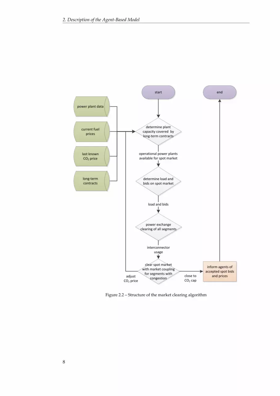
Figure 2.1 provides an overview of the model. Before the start of the simulation, ascenario file is uploaded which specifies the (random functions of) time series data (suchas fuel prices), demand functions, generation technologies, generation portfolio’s and theparameters of policy instruments such as the CO2 cap or tax level. Within each time step(which is one year), the electricity markets are cleared for each section of the load-durationfunction. If a CO2 market is implemented, the CO2 price is determined in an iterativeprocess with electricity market clearing: the price is adjusted until the emissions just matchthe cap. Each time step, agents also decide whether to invest in new plant and whether todismantle old plant and they buy CO2 credits, if applicable.

2.2 Agents

The main agents in the model are the electricity generation companies. In addition, ag-Strategic decisions ofproducers gregate electricity consumption is represented by a single agent. The number of power

generation companies can be chosen by the modeler, as well as the size and consistency oftheir power plant portfolios at the start of the simulation. The generation companies needto make the following types of strategic decisions:

• Investment. The agents decide whether investing in a new power generation facilityis sufficiently attractive to them. Agents invest when a new power plant appearsattractive enough; see Section 2.7 for a description of the investment algorithm.

• Technology type. If agents decide to invest, they need to choose a type of electricitygeneration technology.

4

2.2. Agents, April 26, 2013

behavior

engine

medium time scale behaviorlong time scale behavior

select scenario

start

initialize simulation

selection

agents, behavior, data, exogenous

variables, policies

CO2 auction and electricity

spot market

invest ingeneration

capacity

dismantlegeneration

capacity

clear fuel markets

commit to long-term contracts

short time scale behavior

determine fuel mix

unit dispatch

market coupling

end

simulation done

time controller

simulation ready

to analysis

progress

to dashboard

graph database containing the

state

signlong-term contracts

Figure 2.1 – Structure of the model

5

2. Description of the Agent-Based Model

Apart from strategic management, power generators make the following operationalGenerators’ operationaldecisions decisions:

• Sell electricity. Generation companies offer their electricity to the power exchange atmarginal cost plus a price markup, which is assumed to exist due to market power.The marginal cost of generation is derived from fuel and CO2 prices.

• Purchase fuel. Based on actual electricity production, the required fuel is determinedand acquired. In case of multi-fuel power plants, agents optimise their fuel consump-tion based on expected fuel prices.

• Acquire CO2 emission rights. The volume of CO2 emission rights that generationcompanies purchase is determined in an iterative process in which the arbitrage be-tween the electricity and CO2 markets is optimized. See Section 2.6 for a description.The assumption is that the short-term electricity and CO2 markets work optimallyand that arbitrage between them also is optimal.

A single consumer agent represents the aggregate demand of all domestic consumersConsumer agent

for electricity. The yearly demand depends on the scenario (see below).

2.3 Generation technologies

There is no restriction on the number of electricity generation technologies that can beAvailable technologies

used in this model. For simplicity’s sake, however, we start the model with the followingtechnologies.

• Coal (with optional biomass co-firing) with and without CCS

– Pulverised Super Critical (PSC)– Integrated Gasification Combined Cycle (IGCC)

• Biomass• Gas

– Open Cycle Gas Turbine (OCGT)– Combined Cycle Gas Turbine, with and without CCS (CCGT)

• Nuclear Power• Wind

– Onshore– Offshore

• Photovoltaic

The main attributes of power plants that are modeled are fuel efficiency, investmentcost, operating and maintenance (O&M) cost, maximum load, lifetime and constructiontime.

We use typical cost and technology characteristics of existing generation plants (or, inInnovation

case of coal with CCS, a plausible estimate). The specific assumptions are described inAppendix A. In the model, the efficiency of new power plants improves gradually overtime (resulting in lower fuel consumption and CO2 output per MWhe produced). For newtechnologies such as wind and CCS, these learning rates develop more quickly than forexisting ones. Capital and operating costs of new plants also decline, but during the courseof a plant’s lifetime, its fixed operating and maintenance costs increase, first graduall andthen more strongly after its nominal life span has elapsed.

6

2.4. Intermittent energy sources, April 26, 2013

2.4 Intermittent energy sources

Intermittent energy sources such as wind and solar energy present a challenge to a long- Short-term effects in along-term modelterm model. In order to represent prices and the need for capacity realistically, the inter-

mittancy of wind needs to be represented in the model. This is a short-term effect, but inorder to reduce run-time and complexity, the model abstracts from the details of short-termpower system operation and price formation. However, the effects of intermittent sourceson prices and the load factor of thermal plant cannot be ignored. As the availability ofthese resources cannot be controlled, their contribution to meeting peak generation capac-ity needs is limited. Instead, we model the impact that intermittent resources have on eachstep of the load-duration function.

Approximation ofintermittencyIn our model, we approximate this effect by letting intermittent resources contribute dif-

ferent ratios of their nameplate capacity for different segments of the load-duration curve.To take onshore wind as an example, it only contributes 5% of its capacity during peakhours, but up to 40% of their nameplate capacity during the lowest segment of the load-duration function. In the load-duration segments in between, the contribution of intermit-tent resources is scaled linearly, and calibrated in such a way, that full load hours duringone year correspond to empirical values. In this way, When there is much investment inintermittent resources, the model will reflect the limited contribution to peak generationcapacity, while the load factor of fossil plants will decrease.

2.5 Power plant operation and spot market bidding

Generation companies dispatch their power stations in strict merit order. Outages, start- Dispatch

up costs and ramp rates are not considered. They base their bids in the market on theavailable capacity and the variable costs (including the price of CO2) of their plants. Sometypes of power plant can run on multiple fuels. A common example is coal with biomass,but more innovative technologies such as multi-fuel natural gas/coal gasification/biomassgasification plants can be added. The fuel dispatch of these plants is optimized for fuel andCO2 prices and the energy densities of the fuels.

The fuel mix of multi-fuel power plants is determined at the beginning of each year,implicitly assuming that this is the time that fuel supply contracts are concluded. As aconsequence of this assumption the CO2 price is not known, and the agents take the pre-vious year’s CO2 price as a best estimate to calculate their optimal fuel mix. This is donevia a linear program taking into consideration current fuel prices (which are known), lastyear’s CO2 price, the power plant efficiency and the fuel mix constraints given in Table A.2.The resulting variable fuel costs per MWhel for power plant p are then determined as theweighted average of the fuel prices:

cp, f uel = ∑f

p f · sp, f

ηp,e(2.1)

Assuming that variable power plant costs are solely determined by their fuel costs, andthat all generators can exercise market power, the bidding strategy (cf. equation 2.3) for allagents is defined as:

pc,s,p,t = cp, f uel · (1 + mg) (2.2)

We assume the price mark-up to be 10% for all generators, following the example of ?.

2.6 The electricity and CO2 market algorithms

In this section we will describe how the electricity and CO2 markets are cleared. The Overview of IterativeProcess

7

2. Description of the Agent-Based Model

determine load and bids on spot market

start

close to CO2 cap

end

inform agents of accepted spot bids

and prices

determine plant capacity covered by long-term contracts

operational power plants available for spot market

load and bids

power exchangeclearing of all segments

clear spot market with market coupling

for segments with congestion

interconnector usage

adjust CO2 price

current fuel prices

last known CO2 price

power plant data

long-term contracts

Figure 2.2 – Structure of the market clearing algorithm

8

2.6. The electricity and CO2 market algorithms, April 26, 2013

time step of the model is one year. There are 2 interconnected electricity markets with 5generators, distributed over these markets. Electricity demand is represented by a step-wise load-duration function which is different per modeled price zone. Electricity pricesmay thus vary between markets if the interconnector is congested. The number of stepscan be varied in the model; the higher the number, the more refined the representationof demand, but the slower the model. The supply function is constructed by placing thegenerator bids in merit order. Generators base their bids on the price of CO2 (in the firstiteration, this is the previous year’s CO2 price) and the exogenously determined fuel prices.CO2 emissions are constrained by the annual emissions cap. As perfect trade in CO2 isassumed between these markets, so that the CO2 price is the same in all markets in themodel. It is assumed that the ’consumption’ of CO2 credits can be arbitraged perfectlybetween the different hours of a year; therefore, there is only one CO2 price in each year.An iterative process is used to find the market prices of electricity and CO2. Given a certainstarting value of the CO2 price, the markets are cleared. When the emissions are higher thanthe cap, the CO2 price is increased and vice versa. The electricity markets are cleared again,with the different CO2 price leading to an adjustment in emissions. This process is repeateduntil the CO2 emissions are equal to the emissions cap. Figure 2.2 on page 8 provides anoverview of the electricity and CO2 market clearing algorithm, and the different steps aredescribed in more detail below.

The generators bid into each of the segments, using one price-volume pair per segment Electricity MarketBiddingand power plant. The electricity market they bid into is determined by the location (country

c) of the power plant p. The bidding strategy is described in Section 2.5.

bc,s,p,t = (pc,s,p,t, Vc,s,p,t) (2.3)

The bids of the power generators are than universally adjusted for a given, identical CO2 Price adjustment

CO2 price pCO2 and the complimentary CO2 tax TCO2,C, as well as the the emission intensityep of the power plant, so that the costs of CO2 emission are accounted for in the bid. In thefirst iteration round, the CO2 price of the last year is taken.

bCO2c,s,p,t = (pc,s,p,t + (pCO2 + TCO2,c,t) · ep, Vc,s,p,t) (2.4)

The complimentary tax is set such that the minimum CO2 price floor FCO2,c in Country c isguaranteed:

TCO2,c = max(0, FCO2,c,t − pCO2) (2.5)

In principle, the electricity markets in the model are than cleared the same way as real Electricity marketclearingpower exchanges. For each segment in the load-duration function, price and volume are

determined by the intersection of supply and demand. The generator bid pairs includingthe CO2 costs are sorted from low to high price and the intersect of the resulting supplyfunction with demand (which is presumed inelastic) determines the price and volume ofelectricity sold. The markets are cleared independently for every step of the load-durationfunctions, yielding a step-wise price-duration function with the same number of steps asthe load-duration function. In each segment the highest accepted bid (that is needed tosatisfy demand) bCO2,∗

s,p,t = (ps,p,t, V∗s,p,t) sets the market clearing price ρs,t for segment s. Incase demand Ds,t in segment s cannot be satisfied, the clearing price is set to the value oflost load.

The market clearing algorithm, as described above, is first run for all zones in the model Congestionmanagementtogether. This implies the assumption that there is no congestion between the zones and

results in a single electricity price for all zones together. If the resulting flows over theinterconnectors exceed available capacity, the congestion is managed by means of marketsplitting. (In the simplified environment of this model, the outcome is the same as if marketcoupling were applied.) We will now describe the congestion management algorithm for

9

2. Description of the Agent-Based Model

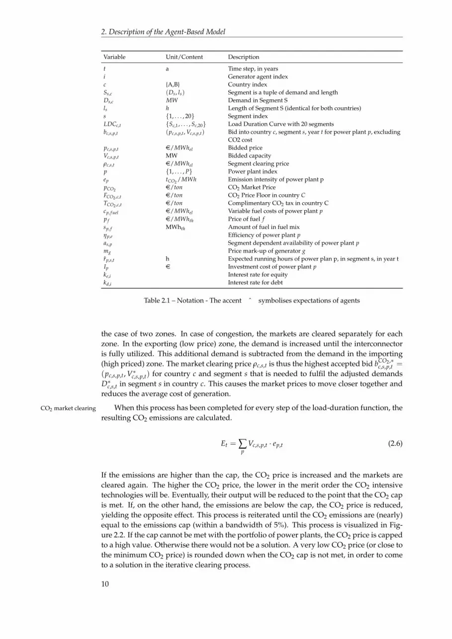
Variable Unit/Content Description

t a Time step, in yearsi Generator agent indexc {A,B} Country indexSs,c (Ds, ls) Segment is a tuple of demand and lengthDs,c MW Demand in Segment Sls h Length of Segment S (identical for both countries)s {1, . . . , 20} Segment indexLDCc,t {Sc,1, . . . , Sc,20} Load Duration Curve with 20 segmentsbc,s,p,t (pc,s,p,t, Vc,s,p,t) Bid into country c, segment s, year t for power plant p, excluding

CO2 costpc,s,p,t e/MWhel Bidded priceVc,s,p,t MW Bidded capacityρc,s,t e/MWhel Segment clearing pricep {1, . . . , P} Power plant indexep tCO2 /MWh Emission intensity of power plant ppCO2 e/ton CO2 Market PriceFCO2 ,c,t e/ton CO2 Price Floor in country CTCO2 ,c,t e/ton Complimentary CO2 tax in country Ccp, f uel e/MWhel Variable fuel costs of power plant pp f e/MWhth Price of fuel fsp, f MWhth Amount of fuel in fuel mixηp,e Efficiency of power plant pas,p Segment dependent availability of power plant pmg Price mark-up of generator grp,s,t h Expected running hours of power plan p, in segment s, in year tIp e Investment cost of power plant pke,i Interest rate for equitykd,i Interest rate for debt

Table 2.1 – Notation - The accent ˆ symbolises expectations of agents

the case of two zones. In case of congestion, the markets are cleared separately for eachzone. In the exporting (low price) zone, the demand is increased until the interconnectoris fully utilized. This additional demand is subtracted from the demand in the importing(high priced) zone. The market clearing price ρc,s,t is thus the highest accepted bid bCO2,∗

c,s,p,t =

(pc,s,p,t, V∗c,s,p,t) for country c and segment s that is needed to fulfil the adjusted demandsD∗c,s,t in segment s in country c. This causes the market prices to move closer together andreduces the average cost of generation.

When this process has been completed for every step of the load-duration function, theCO2 market clearing

resulting CO2 emissions are calculated.

Et = ∑p

Vc,s,p,t · ep,t (2.6)

If the emissions are higher than the cap, the CO2 price is increased and the markets arecleared again. The higher the CO2 price, the lower in the merit order the CO2 intensivetechnologies will be. Eventually, their output will be reduced to the point that the CO2 capis met. If, on the other hand, the emissions are below the cap, the CO2 price is reduced,yielding the opposite effect. This process is reiterated until the CO2 emissions are (nearly)equal to the emissions cap (within a bandwidth of 5%). This process is visualized in Fig-ure 2.2. If the cap cannot be met with the portfolio of power plants, the CO2 price is cappedto a high value. Otherwise there would not be a solution. A very low CO2 price (or close tothe minimum CO2 price) is rounded down when the CO2 cap is not met, in order to cometo a solution in the iterative clearing process.

10

2.7. Investment algorithm, April 26, 2013

2.7 Investment algorithm

In order to come to an investment process, where decisions by generator agents are in- Overview

fluenced by other agents’ actions, the investment are made sequentially in several rounds.The investment process is stopped as soon as no agent is willing to invest any more, i.e.further investments seem unattractive due to already announced power plants. To preventa continuous bias towards agents induced by the investment rounds, the order in whichagents invest is determined randomly in each year. Agents are assumed to finance a partof their investment cost of a power plant from their cash flow, expecting a specific returnon equity ke,i, and finance the remaining investment cost from debt, at an interest rate kd,igiven by the bank. The loan is assumed to be payed back in equal annuities during thedepreciation period of the power plant.

The investment algorithm is based on the assumption that investors would like to in- Principle: NPV forreference yearvest to the point that their investment just makes a profit, but that they do not have perfect

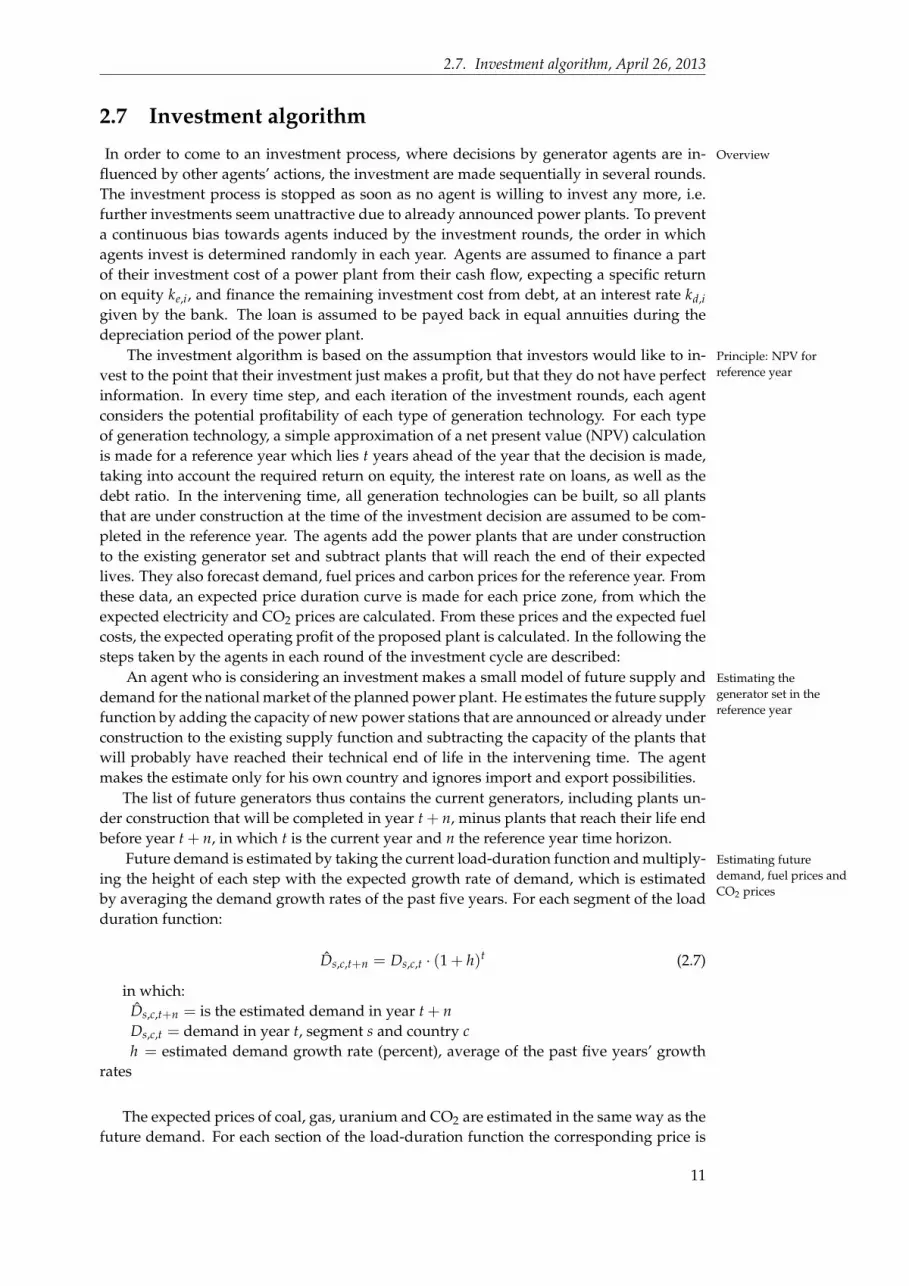
information. In every time step, and each iteration of the investment rounds, each agentconsiders the potential profitability of each type of generation technology. For each typeof generation technology, a simple approximation of a net present value (NPV) calculationis made for a reference year which lies t years ahead of the year that the decision is made,taking into account the required return on equity, the interest rate on loans, as well as thedebt ratio. In the intervening time, all generation technologies can be built, so all plantsthat are under construction at the time of the investment decision are assumed to be com-pleted in the reference year. The agents add the power plants that are under constructionto the existing generator set and subtract plants that will reach the end of their expectedlives. They also forecast demand, fuel prices and carbon prices for the reference year. Fromthese data, an expected price duration curve is made for each price zone, from which theexpected electricity and CO2 prices are calculated. From these prices and the expected fuelcosts, the expected operating profit of the proposed plant is calculated. In the following thesteps taken by the agents in each round of the investment cycle are described:

An agent who is considering an investment makes a small model of future supply and Estimating thegenerator set in thereference year

demand for the national market of the planned power plant. He estimates the future supplyfunction by adding the capacity of new power stations that are announced or already underconstruction to the existing supply function and subtracting the capacity of the plants thatwill probably have reached their technical end of life in the intervening time. The agentmakes the estimate only for his own country and ignores import and export possibilities.

The list of future generators thus contains the current generators, including plants un-der construction that will be completed in year t + n, minus plants that reach their life endbefore year t + n, in which t is the current year and n the reference year time horizon.

Future demand is estimated by taking the current load-duration function and multiply- Estimating futuredemand, fuel prices andCO2 prices

ing the height of each step with the expected growth rate of demand, which is estimatedby averaging the demand growth rates of the past five years. For each segment of the loadduration function:

Ds,c,t+n = Ds,c,t · (1 + h)t (2.7)

in which:Ds,c,t+n = is the estimated demand in year t + nDs,c,t = demand in year t, segment s and country ch = estimated demand growth rate (percent), average of the past five years’ growth

rates

The expected prices of coal, gas, uranium and CO2 are estimated in the same way as thefuture demand. For each section of the load-duration function the corresponding price is

11

2. Description of the Agent-Based Model

current data for new plants

select power plants with

NPV > 0

start

choice

gather alternatives

end

create new power plant, start

construction, pay downpayment

alternatives

determine expected revenues and costs

in base year

expected revenues and costs

past market results,

announced constructions,discount rate

physical and financial

constraints

select power plants withhighest return on

investment

attractive alternatives

no attractive alternatives

Figure 2.3 – Structure of the investment algorithm

12

2.7. Investment algorithm, April 26, 2013

than estimated as the variable cost of the marginal plant. Thus a price-duration function isdetermined that has the same number of steps as the load-duration function (ρc,s,t+n, ∀s).

The first question is whether an agent invests at all. Before considering the question First criterion: financialstatus of companyof which technology might be profitable, an agent (or his financiers) decide whether he is

capable of paying the downpayment (typically 30% of the total capital cost).The expected running hours in each segment rs,p,t+n are determined from the estimated Expected running hours

future energy prices ρc,s,t+n the variable costs cv,p,t+n of the power plant and the segmentdependent availability rate as, which lowers running hours for intermittent renewable tech-nologies. If the plant is expected to be in the merit order, i.e. variable costs are smaller thanexpected prices, the running hours are the product of the segment length ls and segmentdependent availability as.

rs,p,t =

{ls · as , ρc,s,t+n ≥ cv,p,t+n

0 , else(2.8)

The sum of running hours is than compared to the minimum running hours of thegeneration technology, and the investment decision only proceeds if this requirement hasbeen fulfilled.

The agent estimates a plant’s expected cash flow by subtracting the plant’s variable Cash Flow Estimation

costs cv,p,t (based on the estimates of fuel and CO2 costs) from the estimated market priceρc,s,t for each segment s of the load-duration curve. Where the result is negative, the plantdoes not run and operating profits are zero, due to the multiplication with zero runninghours rs,p,t+n (cp. Equation 2.8). This yields the expected operating cash flow in the ref-erence year t + n. For the final cash flow estimation the fixed cost of the power plant aresubtracted.

CFp,t+n = ∑s((ρc,s,t+n − cv,p,t+n) · rs,p,t+n)− c f ,p,t (2.9)

In order compare power plants of different capacities κp with each other, the spe- Discounted Cash Flow

cific project net present value (NPV) of the considered power plant is calculated using theweighted average cost of capital (WACC) as the interest rate. It is assumed that the total in-vestment costs are spread linearly over the building time (0, . . . , tb), and that the cash flowCF is representative for the life time of the power plant (tb + 1, . . . , tb + tD).

NPVp =(

∑t=0...tb

−Ip/(tb + 1)(1 + WACC)t + ∑

t=tb+1...tb+tD

CFp,t+n

(1 + WACC)t

)/κp (2.10)

If positive NPVs exist,the power plant p with the highest specific NPVp per megawatt ischosen for investment.

This investment algorithm is only a first approximation of investment behavior. A num-ber of possible extensions present themselves.

An obvious extension is to calculate the NPV calculated for each year within (a certaintime horizon), as the expected cash flows may vary significantly. The price is that the runtime of the model will increase proportionally.

For better accuracy, cross-border flows should be taken into account in the NPV. This iscomplicated, however, as it would require the agents to make forecasts of the results of thecongestion management in order to estimate their revenues.

The investment decision process itself is more complex than a simple NPV calculation.Subjective factors such as risk aversion and technology preferences could be included inthe future.

13

2. Description of the Agent-Based Model

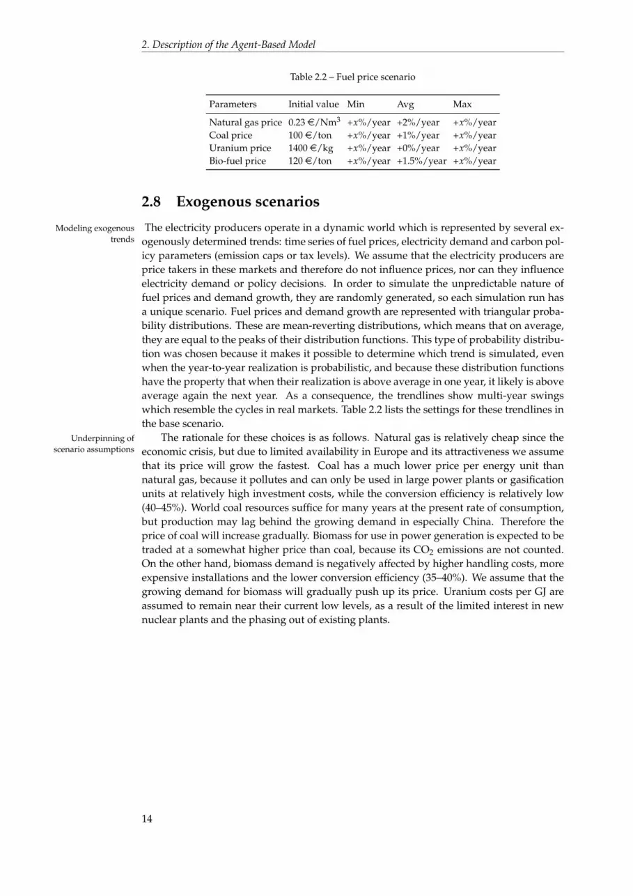
Table 2.2 – Fuel price scenario

Parameters Initial value Min Avg Max

Natural gas price 0.23 e/Nm3 +x%/year +2%/year +x%/yearCoal price 100 e/ton +x%/year +1%/year +x%/yearUranium price 1400 e/kg +x%/year +0%/year +x%/yearBio-fuel price 120 e/ton +x%/year +1.5%/year +x%/year

2.8 Exogenous scenarios

The electricity producers operate in a dynamic world which is represented by several ex-Modeling exogenoustrends ogenously determined trends: time series of fuel prices, electricity demand and carbon pol-

icy parameters (emission caps or tax levels). We assume that the electricity producers areprice takers in these markets and therefore do not influence prices, nor can they influenceelectricity demand or policy decisions. In order to simulate the unpredictable nature offuel prices and demand growth, they are randomly generated, so each simulation run hasa unique scenario. Fuel prices and demand growth are represented with triangular proba-bility distributions. These are mean-reverting distributions, which means that on average,they are equal to the peaks of their distribution functions. This type of probability distribu-tion was chosen because it makes it possible to determine which trend is simulated, evenwhen the year-to-year realization is probabilistic, and because these distribution functionshave the property that when their realization is above average in one year, it likely is aboveaverage again the next year. As a consequence, the trendlines show multi-year swingswhich resemble the cycles in real markets. Table 2.2 lists the settings for these trendlines inthe base scenario.

The rationale for these choices is as follows. Natural gas is relatively cheap since theUnderpinning ofscenario assumptions economic crisis, but due to limited availability in Europe and its attractiveness we assume

that its price will grow the fastest. Coal has a much lower price per energy unit thannatural gas, because it pollutes and can only be used in large power plants or gasificationunits at relatively high investment costs, while the conversion efficiency is relatively low(40–45%). World coal resources suffice for many years at the present rate of consumption,but production may lag behind the growing demand in especially China. Therefore theprice of coal will increase gradually. Biomass for use in power generation is expected to betraded at a somewhat higher price than coal, because its CO2 emissions are not counted.On the other hand, biomass demand is negatively affected by higher handling costs, moreexpensive installations and the lower conversion efficiency (35–40%). We assume that thegrowing demand for biomass will gradually push up its price. Uranium costs per GJ areassumed to remain near their current low levels, as a result of the limited interest in newnuclear plants and the phasing out of existing plants.

14

3 Implementation inAgentSpring

The consequence of policy intervention typically materialize by changing the behavior Policy support

of actors regarding their options, assets and decisions. That is a core reason in favour ofABM, but it also highlights that the scope of models for policy decisions is relatively large.The models need to be rich enough in order to properly represent the social, the technicaland socio-technical components and their interactions (Chappin, 2011). For policy support,elaborate and diverse behavior of agents has to be possible. Models are data driven andhave to incorporate extensive behavior algorithms (Chmieliauskas et al., 2012).

The desire to open up models to a community of researchers, public and private prob- Open access models

lem owners, and the general public is an important approach to ventilate research resultsto the public. It changes the role of models and simulations in the debate, and allows theend user to explore, validate and experiment with the tools that researchers develop. Inaddition, extendability and reusability of code is important, because it allows developedmodels to become a basis around years of policy-supporting modelling research.

3.1 AgentSpring framework

There are many ABM frameworks in existence, some more popular than others. Although Modelling frameworks

it may have been possible to use and modify existing frameworks, we have taken up the op-portunity to build the AgentSpring framework that would leverage off the new and pow-erful open source libraries and changing software development paradigms. AgentSpringis developed as an open-source tool. This implies that anyone can use and contribute tothe platform. AgentSpring is available online1. AgentSpring is based on Java technolo-gies and runs on all popular operating systems (Linux, Windows, and Mac). AgentSpringgets its name from and makes use of Spring Framework – a popular software developmentframework, that promotes the use of object oriented software patterns (Johnson et al., 2009).One such pattern calls for separation of data, logic and user interface (Krasner and Pope,1988). Although the latter is an old concept, most modeling frameworks mix the three.This may be reasonable for creating smaller models, but for a base electricity and CO2model (see the application section) it will be ineffective in the long run. Developing andusing AgentSpring enabled us to build a model that is better maintainable and expandable.

3.2 User interface

AgentSpring is characterized by a web-based user interface. See figure 3.1 for a snapshot of Web-based userinterfacea running model. As a developer, AgentSpring runs as a local webserver (typically located

1AgentSpring can be found at https://github.com/alfredas/AgentSpring. At the time of writing, the currentversion AgentSpring is 1.0.

15

3. Implementation in AgentSpring

Figure 3.1 – Snapshot of the user interface of AgentSpring with the model running

at http://localhost:8080/agentspring-face/). This setup also allows AgentSpring to be ranon a dedicated server that is securely opened up for external visits.

The interface allows to start, pause and stop the model, to change and create graphsby writing queries and to observe a textual log. Additionally, the interface can be used toselect various predefined scenarios and to change key parameters in the model. A modelin AgentSpring can also be controlled from command line, with or without running theAgentSpring user interface.

3.3 The system captured in a database

AgentSpring makes use of special way to contain the state of the modelled system. Themodelled system is captured in a so-called graph database, which is a database that uses agraph structure of nodes, edges, and properties to represent and store information (Eifrem,2009).

The complete state of the system at any point in time is considered a graph of ob-Graph database

jects and their relationships. AgentSpring allows the graph to scale to hundreds of agents,millions of things and relations between them. The application of a database in ABM ispromising as it allows for a different representation of the system modeled: the structure ofthe system – the objects and their interactions/relations – emerges and evolves. Capturingthe data and perserving it in a database, makes it flexible to save and search. It enablesefficient selection and finding by performing appropriate queries.

An example of a query could be to find all electricity spot markets for which theQueries

property valueOfLostLoad is higher than 500 e/MWh load lost and on which the loadDu-rationCurve contains at lest 15 segments (see figure 3.2 for the relational diagram for this

16

3.4. Types of classes and other files, April 26, 2013

Figure 3.2 – The graph of possible relations for an electricity spot market, a relatively small example.The grey box is the starting point. Solid arrows refer to an ‘is a’ relationship. Dashed arrows are eitherproperty or a relation to another object. In this example an ElectricitySpotMarket is a Decarbonization-Market, which is a DecarbonizationAgent. An ElectricitySpotMarket has (or can have) a property calledvalueOfLostLoad, which is a double precision number. It also has the property loadDurationCurve, whichis a set of SegmentLoad objects. Graphs like these are part of the documentation (see below)

example, which is part of the documentation). Traditionally, this would be solved main-taining a list of all spot markets in the model, looping over them and checking piece bypiece for both conditions. A query, however, will be easier to compose, shorter in code, andit will be much faster. These advantages become even more relevant when queries spanvarious types of objects. It also allows for thinking differently about extracting information,both for analysis of a running model as well as for the behavior of agents themeselves. Anexample of a more complicated query would be one that calculates the average efficiencyof all PowerPlants that have a PowerGeneratingTechnology that uses fuels emitting CO2, ofwhich the EnergyProducer agent – the owner – has a positive cash balance.

3.4 Types of classes and other files

AgentSpring uses various types of Java classes and other files.Domain classes are the definitions of things and their properties. For instance it contains Domain classes

the classes Agent and PowerPlant.Role classes capture pieces of behavior, such as InvestInPowerPlantRole, that can be ex- Role classes

ecuted by specific types (or classes) of Agents (which are in the domain, EnergyProducerin this case). Behavior typically results in new or changed information or objects that arepersisted in the database with the help of repositories.

Repository classes contain functions that deal with the interaction of typical model code Repository classes

and the database. For instance, findAllOperationalPowerPlants is a function in the Power-PlantRepository, that executes a query to the database for all power plants, checks whichones are operational (and are not unavailable, under construction or decommissioned),and returns the result. Repositories also assist in updating current information or storingnew information.

Scenario xml files contain all data to define and initiate a simulation run. A scenario Scenario files

contains data, but also relations between objects. An example of data is parameters ofpower plants, and a price trend for coal. An example of a relation that is captured in thescenario is the fact that on a market for trading a specific substance a relation is made to thesubstance coal that can be traded on this particular market. Furthermore, a coal supplying

17

3. Implementation in AgentSpring

agent is connected to the market.

3.5 Modelling agents and their behavior

AgentSpring makes use of the concepts of roles to encode agent behavior in a modularModular behavior

way. Agents play their roles in the simulation by executing their in modules coded behav-ior. Models are made by linking agents to such roles and composing a script that togetherdefine the set of behaviors in the context of social situations. This makes AgentSpringparticularly suited to modeling complex socio-technical systems. AgentSpring decouplesagents, their behaviors and their environments. That enables to reuse the pieces, to com-pose consistent new pieces. Experience has shown that only modular and reusable modelscan accommodate changing scope and new research questions.

The roles that make up the behavior of agents have the following properties:Properties of roles

• A role is enacted by a specific class of agents.

• A role encodes a piece of behavior.

• Input for roles are the properties of the agent enacting the role, but also other parts ofthe system. Queries are used to access the graph database and retrieve the informa-tion needed for the behavior to be executed.

• The outcome of the behavior that is captured in a role implies a change in somethingin the state of the system. This is then stored in the graph database.

• A role can initiate other roles, i.e. a hierarchy of roles can be developed.

• Roles do not interact with each other directly (apart from iniating other roles, see theprevious bullet).

3.6 Development and documentation

Typical software development practices enable version control of model through githubSoftware practices

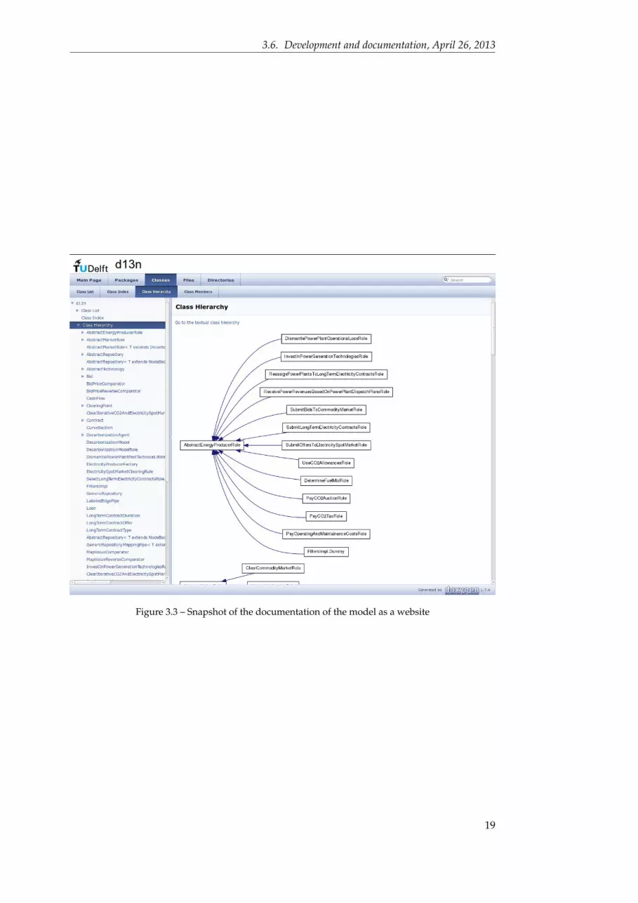
(https://github.com/emlab/emlab-generation for the model described). This is connectedto a wiki-enabled interface to communicate between developers. Another practice in Javacoding is on writing documentation. Online documentation is generated based on thestructure of the code and the documentation written as part of the code. See figure 3.3for a snapshot of the online documentation. The documentation is intuitive enough to findyour way and grasp both the structure and details of model in multiple ways. Links be-tween classes are visualized and linked and for each function a graph is made what otherfunctions it uses and it is used by. The documentation supports modellers and the commu-nity around models to understand and explore the structure of the model. It also enables aplatform to think about changes and different scenarios.

18

3.6. Development and documentation, April 26, 2013

Figure 3.3 – Snapshot of the documentation of the model as a website

19

3. Implementation in AgentSpring

20

Appendices

21

A Power plant and fuel data

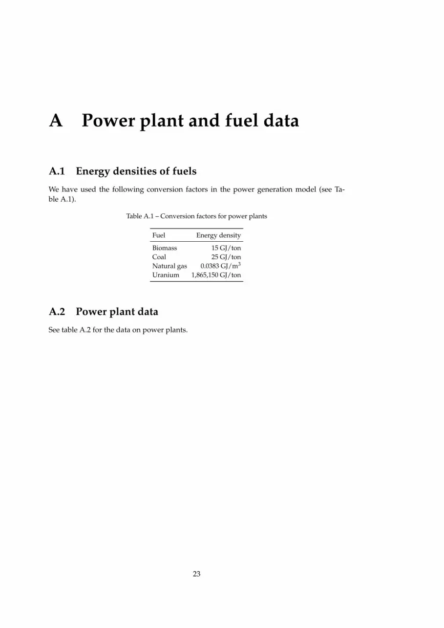
A.1 Energy densities of fuels

We have used the following conversion factors in the power generation model (see Ta-ble A.1).

Table A.1 – Conversion factors for power plants

Fuel Energy density

Biomass 15 GJ/tonCoal 25 GJ/tonNatural gas 0.0383 GJ/m3

Uranium 1,865,150 GJ/ton

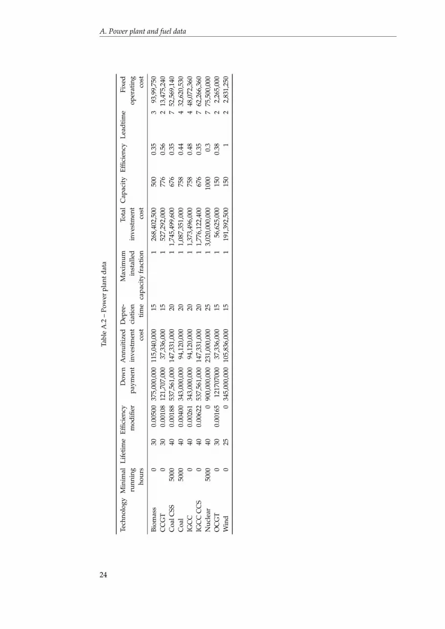
A.2 Power plant data

See table A.2 for the data on power plants.

23

A. Power plant and fuel data

Tabl

eA

.2–

Pow

erpl

antd

ata

Tech

nolo

gyM

inim

alLi

feti

me

Effic

ienc

yD

own

Ann

uiti

zed

Dep

re-

Max

imum

Tota

lC

apac

ity

Effic

ienc

yLe

adti

me

Fixe

dru

nnin

gm

odifi

erpa

ymen

tin

vest

men

tci

atio

nin

stal

led

inve

stm

ent

oper

atin

gho

urs

cost

tim

eca

paci

tyfr

acti

onco

stco

st

Biom

ass

030

0.00

500

375,

000,

000

115,

040,

000

151

268,

402,

500

500

0.35

393

,99,

750

CC

GT

030

0.00

108

121,

707,

000

37,3

36,0

0015

152

7,29

2,00

077

60.

562

13,4

75,2

40C

oalC

SS50

0040

0.00

188

537,

561,

000

147,

331,

000

201

1,74

5,49

9,60

067

60.

357

52,5

69,1

40C

oal

5000

400.

0040

034

3,00

0,00

094

,120

,000

201

1,08

7,35

1,00

075

80.

444

32,6

20,5

30IG

CC

040

0.00

261

343,

000,

000

94,1

20,0

0020

11,

373,

496,

000

758

0.48

448

,072

,360

IGC

CC

CS

040

0.00

622

537,

561,

000

147,

331,

000

201

1,77

6,12

2,40

067

60.

357

62,2

66,3

60N

ucle

ar50

0040

090

0,00

0,00

023

1,00

0,00

025

13,

020,

000,

000

1000

0.3

775

,500

,000

OC

GT

030

0.00

165

1217

0700

037

,336

,000

151

56,6

25,0

0015

00.

382

2,26

5,00

0W

ind

025

034

5,00

0,00

010

5,83

6,00

015

119

1,39

2,50

015

01

22,

831,

250

24

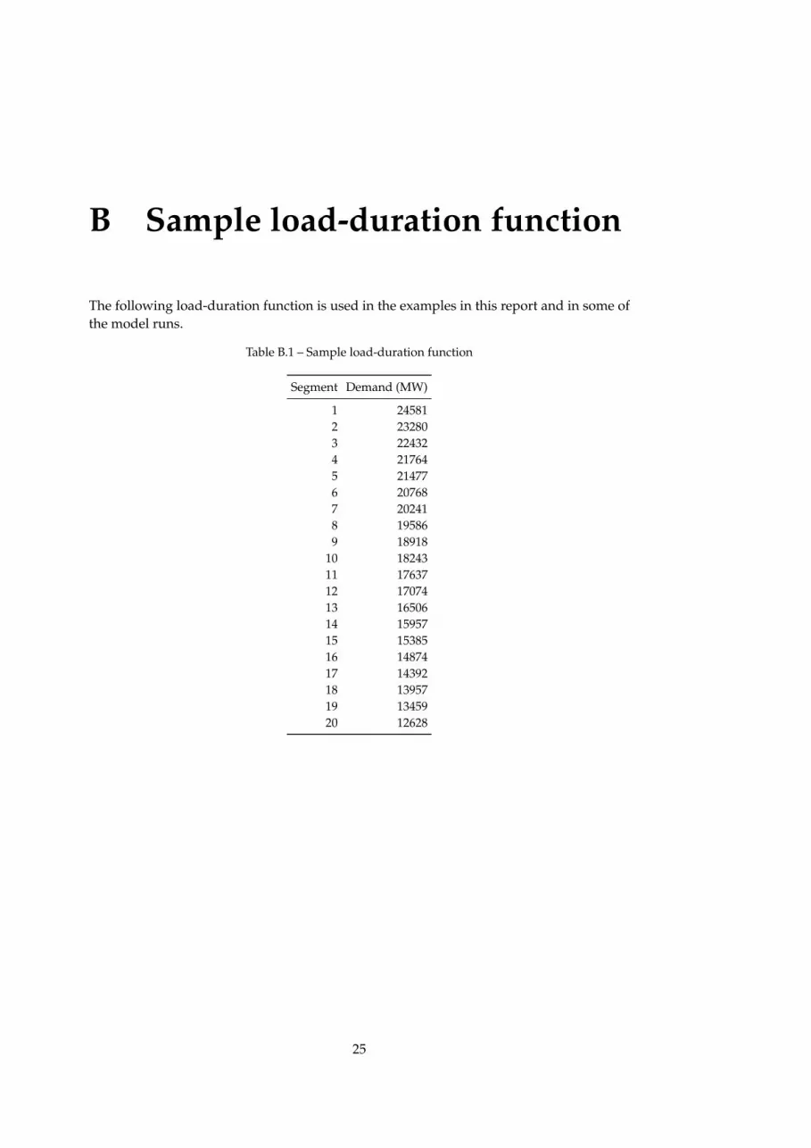
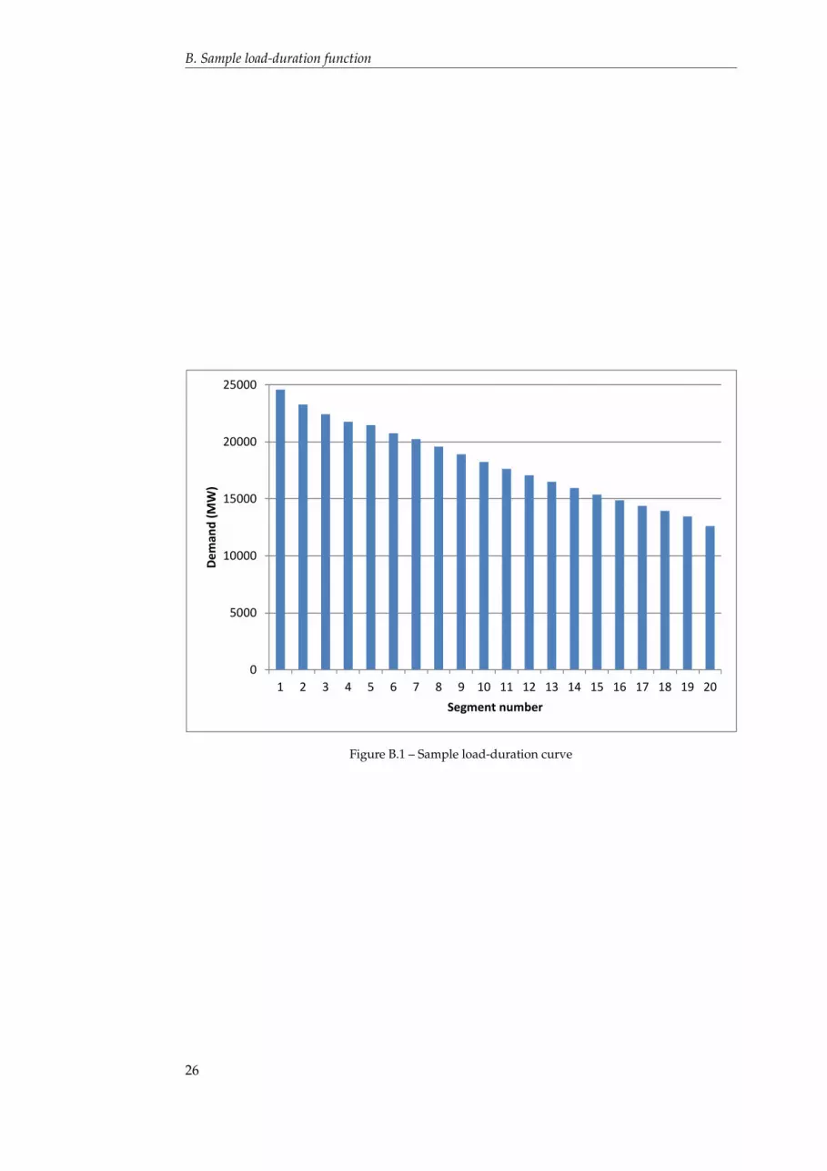
B Sample load-duration function

The following load-duration function is used in the examples in this report and in some ofthe model runs.

Table B.1 – Sample load-duration function

Segment Demand (MW)

1 245812 232803 224324 217645 214776 207687 202418 195869 18918

10 1824311 1763712 1707413 1650614 1595715 1538516 1487417 1439218 1395719 1345920 12628

25

B. Sample load-duration function

0

5000

10000

15000

20000

25000

1 2 3 4 5 6 7 8 9 10 11 12 13 14 15 16 17 18 19 20

Dem

and

(MW

)

Segment number

Figure B.1 – Sample load-duration curve

26

Acknowledgements

This work was supported by the Energy Delta Gas Research program, project A1 – Under-standing gas sector intra-market and inter-market interactions and by the Knowledge forClimate program, project INCAH – Infrastructure Climate Adaptation in Hotspots.

27

Acknowledgements

28

Bibliography

Chappin, E. J. L. (2011). Simulating Energy Transitions, PhD thesis, Delft University of Tech-nology, Delft, the Netherlands. ISBN: 978-90-79787-30-2.URL: http://chappin.com/ChappinEJL-PhDthesis.pdf 15

Chappin, E. J. L., Chmieliauskas, A. and de Vries, L. J. (2012). Agent-based models forpolicy makers, ESSA 2012 – 8th Conference of the European Social Simulation Association,University of Salzburg, Salzburg, Austria. 2

Chmieliauskas, A., Chappin, E., Davis, C., Nikolic, I. and Dijkema, G. (2012). New methodsin analysis and design of policy instruments, in A. V. Gheorghe (ed.), System of Systems,Intech. 15

Eifrem, E. (2009). Neo4j - the benefits of graph databases, no: sql (east) . 16

Johnson, R., Hoeller, J., Arendsen, A. and Thomas, R. (2009). Professional Java Developmentwith the Spring Framework, Wiley-India. 15

Krasner, G. E. and Pope, S. T. (1988). A cookbook for using the model-view controller userinterface paradigm in smalltalk-80, J. Object Oriented Program. 1(3): 26–49. 15

29