Mixing by porous media

This article appeared in a journal published by Elsevier. The attachedcopy is furnished to the author for internal non-commercial researchand education use, including for instruction at the authors institution

and sharing with colleagues.

Other uses, including reproduction and distribution, or selling orlicensing copies, or posting to personal, institutional or third party

websites are prohibited.

In most cases authors are permitted to post their version of thearticle (e.g. in Word or Tex form) to their personal website orinstitutional repository. Authors requiring further information

regarding Elsevier’s archiving and manuscript policies areencouraged to visit:

http://www.elsevier.com/copyright

http://www.elsevier.com/copyright

Author's personal copy

C. R. Mecanique 340 (2012) 933–943

Contents lists available at SciVerse ScienceDirect

Comptes Rendus Mecanique

www.sciencedirect.com

Out of Equilibrium Dynamics

Mixing by porous media

Emmanuel Villermaux 1

Aix Marseille Université, IRPHE, 13384 Marseille cedex 13, France

a r t i c l e i n f o a b s t r a c t

Article history:Available online 17 November 2012

Keywords:Porous mediaMixingStatistical distributions

This article reports on a set of simple remarks to understand the fine structure of ascalar mixture advected in a random, interconnected, frozen network of paths, i.e. a porousmedium. We describe in particular the relevant scales of the mixture, the kinetics of theirevolution, the nature of their interaction, and the scaling laws describing the coarseningprocess of the concentration field as it progresses through the medium, including itsconcentration distribution.

© 2012 Published by Elsevier Masson SAS on behalf of Académie des sciences.

1. A mixture in a porous medium

Fig. 1 shows an instantaneous image of a scalar field (the concentration of a diffusive dye carried by the fluid) resultingfrom the advection of an initially straight and uniform line parallel to the left side of the image in a stationary, two-dimensional synthetic porous medium [1,2]. The mean flow going from left to right with velocity u is sustained by aconstant negative pressure gradient in the x direction [3].

One may portrait the different spatial scales apparent in the field in the following way: The initial size s0 at whichthe line is ‘chopped-off’ compares with the correlation length of the medium permeability. Because the velocity fluctuatesrandomly (with a correlation length λ much larger than s0, [1]), the line distorts into a ‘brush’ with a typical streamwisewidth σ , increasing in time. The brush is made of a collection of parallel, corrugated strips, aligned on average with thedirection of the mean flow. The transverse width s of the stretched strips in the brush first shrinks and then, after a mixingtime, broadens by diffusion. Then adjacent strips merge by neighbor coalescence (percolation), thus forming bundles whosetransverse size ξ increases dramatically at the percolation threshold.

The aim of this article is to rationalize the way these different scales are coupled to each other, and derive predictionsfor their scaling laws.

2. Mixing in a nutshell

Take a blob of dyed fluid deposited in a medium of the same fluid. We discuss below in simple terms the time it takesfor the blob’s concentration to vanish in the diluting medium, and how this time depends on the fluid’s underlying motions.The reader is invited to consult e.g. [4–10], for details and applications.

2.1. Rules of thumb

First, in the absence of stirring, that is in the pure diffusion limit on a still substrate, an obvious spatial scale is the initialsize s0 of the blob. The concentration θ in the blob has appreciably decayed from its initial value when the blob has been

E-mail address: [email protected] Also at: Institut Universitaire de France.

1631-0721/$ – see front matter © 2012 Published by Elsevier Masson SAS on behalf of Académie des sciences.http://dx.doi.org/10.1016/j.crme.2012.10.042


934 E. Villermaux / C. R. Mecanique 340 (2012) 933–943

Fig. 1. A definition sketch of the different spatial scales apparent in a mixture advected in a porous medium (see Section 1). Adapted from Le Borgneet al. [2].

Fig. 2. Sketch of an isolated stretched scalar lamella being compressed in its transverse direction z at a rate −s/s, and associated concentration profileθ(z, t) in the local frame of reference of (3) where the direction z concentrates most of the scalar gradient, that is ∂zθ = z ·∇θ , and ∂w θ ≈ 0.

smeared by diffusion, that is when its current radius√

Dt is appreciably larger than s0 and this happens when t � s20/D if

D is the scalar diffusion coefficient.Then, with stirring, the picture is substantially altered. Diffusive smearing is hasten in the presence of stretching because

the scalar gradient (∂zθ(z, t) in Fig. 2) is constantly steepened by compression. Stretching motions are accompanied, inincompressible fluids, by compressive motions. The scalar concentration is close to uniform along the stretching direction,and varies rapidly along the compressive one, thus forming a sheet, or lamella-like topology [11,12]. This, in turn, also setsa characteristic equilibrium scale in the field itself. Let s be the distance between two material points aligned with thecompressive direction z (Fig. 2). The reduction of the width of the lamellae concentration profile goes on until the rate ofcompression −s/s balances the rate of diffusive broadening on its current size D/s2, that is

D

s2∼ −1

s

ds

dt(1)

and when this equilibrium is eventually reached, the lamellae concentration starts to decay. More precisely, on a movingsubstrate, the diffusion equation

∂tθ + u ·∇θ = D∇2θ (2)

simplifies if written in a moving frame {w, z} whose axis is aligned with the directions of maximal stretching and compres-sion of the lamellae where u = {−(s/s)w, (s/s)z}, according to

∂tθ + (s/s)z∂zθ = D∂2z θ (3)

expressing that concentration gradients along the lamellar structures formed by the stretch ∂wθ are essentially zero (seeFig. 2), and concentrate across the lamellae in the direction z aligned with the principal axis of its compression. Thisequation, where the medium disorder appears through the apparent stretching rate −s/s only, is solved in closed form (seeMeunier and Villermaux [10]). Taking for instance a generic form for s(t) as


E. Villermaux / C. R. Mecanique 340 (2012) 933–943 935

s(t) = s0

(1 + γ t

β

)−β

(4)

where γ is a constant elongation rate and β is some positive number. Note that exponential stretching is achieved for largeβ since

s(t) −→β→∞ s0e−γ t (5)

The equilibrium condition (1) is realized at the mixing time ts such that

γ ts ∼ β Pe1/(2β+1) for Pe = γ s20

D� 1 (6)

where Pe denotes the Péclet number (γ ts ∼ 12 ln Pe for β → ∞). The typical width of the scalar gradient which ‘dissipates’

the concentration differences equals

s(ts) ∼ s0(σ ts)−β = s0 Pe−β/(2β+1) (7)

in the large Péclet number limit (when β is also large), one has s(ts) = √D/γ , usually called the Batchelor scale [13]. From

this characteristic time ts , the thickness s increases by simple diffusion (the rate of compression, which diminishes in timelike β/t is now too weak to compensate it)

s(t � ts) ∼ √Dt (8)

and the maximal concentration in the sheet θ(0, t) such that, by mass conservation on an incompressible substrate θ(0, t)×√Dt × (γ t)β is constant, thus decreases like

θ(0, t) ∼ (t/ts)−β−1/2 (9)

2.2. Simple shear with one direction of elongation

Many flows in two dimensions present a persistent shear and increase the length of material lines in proportion to timeas γ t (see e.g. [5,14,8]). This is the case β = 1 above and thus

s = s0

1 + γ tfor t < ts, and s ∼ √

Dt for t � ts (10)

with the mixing time

ts ∼ 1

γPe1/3 with Pe = γ s2

0

D� 1 (11)

providing

θ(0, t) ∼ (t/ts)−3/2 for t > ts (12)

These scaling laws hold when the substrate deformation is faster than diffusion smearing (i.e. Pe � 1 at the pore size s0).They may apply to porous media in the limit of very large macroscopic Péclet numbers (since we already require that Pemust be large at the pore size). Phenomena occurring for Pe � 1, like those described by Taylor [15,16] and Aris [17] for thediffusion in straight tubes, are not directly relevant here, although we will nevertheless invoke diffusion transverse to thestreamlines.

3. Lengthscales and their dynamics

3.1. Large scale dispersion

At scales larger than the ‘pore size’ s0, the position x(t) of a particle in the medium may be represented according to asimple Langevin dynamics{

x(t) = u + f (t)⟨f (t)

⟩ = 0 and⟨f (t) f

(t′)⟩ =Dγ e−γ |t−t′| (13)

where u stands for the mean drift velocity, and f (t) is meant to mimic the fluctuations in velocity due to the convolutedstructure of the medium. This noise reflects the distribution of the permeabilities sampled by a particle along its path, andis conveniently represented here as a random noise, with memory. The memory time γ −1 is equal to the correlation timeof the velocity itself, namely



γ ∼ u/λ (14)

Note that γ e−γ |t−t′ | γ →∞−→ δ(t − t′) so that (13) actually models an advected pure Brownian noise in the large γ limit. Thediffusion coefficient D is, classically, given by the mean free path λ times the particle mean velocity as

D ∼ uλ = γ λ2 (15)

and indeed (13) solves into

σ 2 = ⟨x2⟩ − 〈x〉2

= 2D(

t − 1

γ

(1 − e−γ t)) (16)

with 〈x〉 = ut , giving σ ∼ ut for γ t � 1 (ballistic regime) and σ ∼ √Dt = λ√

γ t for γ t � 1 (diffusive regime).This sketch has many drawbacks, the worst of them being probably that it predicts a Gaussian dispersion front at large

times (γ t � 1) which is often not a good caricature of actual fronts. Indeed if all particles are initially confined into a line ofwidth s0 tagged perpendicular to the mean flow direction x, the resulting mean concentration profile C(x, t) of the particleswill be

C(x, t) ∼ s0√2πσ 2

e− (x−〈x〉)2

2σ2 (17)

This simple model does not account either for a possible slow release of the particle from traps or boundary layers, norfor possible strong bypasses like in fractured media [18–20]. But at least it represents well the time evolution of the twofirst moments of the distribution of the particles positions in the limit of moderate geometric dispersion (i.e. not too broaddistribution of local permeabilities [21,22]), even though if the crossover from the ballistic σ ∼ t to the diffusion regimeσ ∼ √

t is often very broad in practice. In any case, that dispersion has a geometrical origin; this is not Taylor [15] dispersion.

3.2. Microscopic convection–diffusion

By ‘microscopic’, we mean scales of the order of λ, and below. There, particles experience a simple shear between regionsof the flow with different velocities (of the order of u), those being separated by λ, precisely. In fact, velocity fluctuationsdo exist at scales smaller than λ as well, at least down to the scale s0 characteristic of the pore structure (the correlationlength of the permeability). For instance, in a porous medium, the adherence condition at the pore wall will force a line todeform into a set of adjacent strips separated by s0.

The convection diffusion problem is thus likely to fall in the category recalled in Section 2.2 for which of blob of initialtransverse size s0 is elongated linearly in time while keeping its initial concentration up the mixing time (11) after what itsconcentration decays and its typical width measured by the variance of the transverse concentration profile

s2 =∫

z2θ(z, t)dz∫θ(z, t)dz

(18)

increases by molecular diffusion according to (10), that is

s ∼ √Dt (19)

The overall evolution of s (which can be computed exactly from the rigorous convection diffusion problem, see Duplat andVillermaux [9]) may be represented (noting that if s = s0/(1 + γ t) from the flow kinematics, then s = −γ s/(1 + γ t)) as

ds

dt= − γ s

1 + γ t+ D

s(20)

providing

s

s0=

√2(1 + γ t)3 − 2 + 3 Pe

3 Pe(1 + γ t)2−→

t/ts�1

√Dt

s0(21)

This process is likely to last for a long time (in units of λ/u) since the reorientations of the shear are typically unfrequent.The relevant shear is the mean shear u/λ, aligned with the direction of the mean flow.



Fig. 3. Evolution of the lamella thickness s (black) given in (21), its asymptotic trend (∼ t1/2, dotted line), the bundle correlation length ξ (red) given in(23) and the front dispersion width σ (blue) given in (16) all scaled by s0, as a function of time, for Pe = 100. Also singled out in the figure axis are themixing time γ ts and the lamella thickness s(ts).

3.3. Collective dynamics: percolation

A line initially tagged in the medium in a direction perpendicular to the mean flow is thus soon resolved into a set ofparallel lamellae (for γ t > 1) spaced by λ whose width s broadens (for γ ts > 1).

It is clear that when s > λ, all the lamellae are interconnected, thus forming a bundle of uniform concentration whosetransverse width compares with the height of the domain, or with σ (assuming that longitudinal and transverse correlationlengths of the velocity are of the same order).

When s < λ, the probability p that two adjacent lamellae, each of thickness s, overlap is, assuming that the lamellae arelocated at random in the interval λ, given by

p ∼(

s

λ

)2

(22)

corresponding to the square of the relative space occupied by each lamella in λ for this binary collision process. One maydefine a correlation length ξ for the concentration field by writing that the probability that r/λ adjacent lamellae have allmerged is pr/λ , thus defining the correlation function for the concentration e−r/ξ . Then

ξ

λ∼ − 1

ln p(23)

When p → 1, the medium is smooth at the scale λ, and all the lamellae have merged into and large bundle (‘infinitecluster’ in the language of percolation2 (Stauffer [23])). Fig. 3 summarizes these trends. In particular, the time correspondingto p ≈ 1 when the medium starts to be uniform in space is, from (21) and (22)

tu ∼ λ2

D(24)

as would have lead a naive estimate ignoring the interplay between stirring and mixing at the microscopic scale!

3.4. Analogies and differences with deformable media (fluids)

Folding motions coupled to stretching are central to the kinematics of randomly stirred deformable media, like fluids.However, the rigid backbone of a porous medium will not fold (unless it could be deformed as well, like a sponge forinstance, but these folds should be made externally, and would not be the result of the flow itself anyway, unlike in fluids).The scalar field in a porous medium is more like a bundle of parallel, unidirectional strips, rather than an isotropic set ofentangled lamellae. Fig. 4 and Table 1 summarize the analogies and the (important) differences between the two situations.

The microscopic diffusion problem is analogous, in its principle, both in the ‘frozen disorder’ of a porous medium, andin a randomly stirred fluid, when the substrate on which the convection diffusion problem occurs is itself deforming as awhole. The coarsening scale (the analogue of the present ξ , see Villermaux and Duplat [24]) obtained there results from themerging of lamellae (or sheets in three-dimensional flows) on a compressed substrate is steady in time, and smaller that λ.Whereas the dimensions of a porous medium are fixed in time, and the coarsening scale increases, by percolation, with nobound.

2 The above treatment can be refined to account for finite size effects if the bundle cannot be larger than σ .



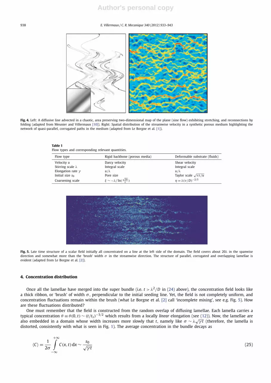
Fig. 4. Left: A diffusive line advected in a chaotic, area preserving two-dimensional map of the plane (sine flow) exhibiting stretching, and reconnections byfolding (adapted from Meunier and Villermaux [10]). Right: Spatial distribution of the streamwise velocity in a synthetic porous medium highlighting thenetwork of quasi-parallel, corrugated paths in the medium (adapted from Le Borgne et al. [1]).

Table 1Flow types and corresponding relevant quantities.

Flow type Rigid backbone (porous media) Deformable substrate (fluids)

Velocity u Darcy velocity Shear velocityStirring scale λ Integral scale Integral scaleElongation rate γ u/λ u/λ

Initial size s0 Pore size Taylor scale√

νλ/u

Coarsening scale ξ ∼ −λ/ ln(√

Dtλ

) η = λ(ν/D)−2/5

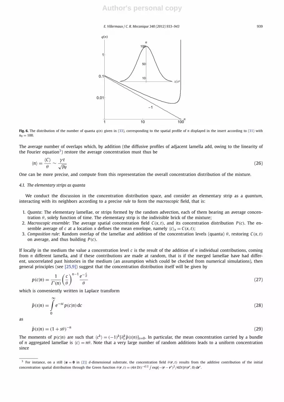
Fig. 5. Late time structure of a scalar field initially all concentrated on a line at the left side of the domain. The field covers about 20λ in the spanwisedirection and somewhat more than the ‘brush’ width σ in the streamwise direction. The structure of parallel, corrugated and overlapping lamellae isevident (adapted from Le Borgne et al. [2]).

4. Concentration distribution

Once all the lamellae have merged into the super bundle (i.e. t > λ2/D in (24) above), the concentration field looks likea thick ribbon, or ‘brush’ of width σ , perpendicular to the initial seeding line. Yet, the field is not completely uniform, andconcentration fluctuations remain within the brush (what Le Borgne et al. [2] call ‘incomplete mixing’, see e.g. Fig. 5). Howare these fluctuations distributed?

One must remember that the field is constructed from the random overlap of diffusing lamellae. Each lamella carries atypical concentration θ ≡ θ(0, t) ∼ (t/ts)

−3/2 which results from a locally linear elongation (see (12)). Now, the lamellae arealso embedded in a domain whose width increases more slowly that t , namely like σ ∼ λ

√γ t (therefore, the lamella is

distorted, consistently with what is seen in Fig. 1). The average concentration in the bundle decays as

〈C〉 = 1

2σ

+∞∫−∞

C(x, t)dx ∼ s0√γ t

(25)



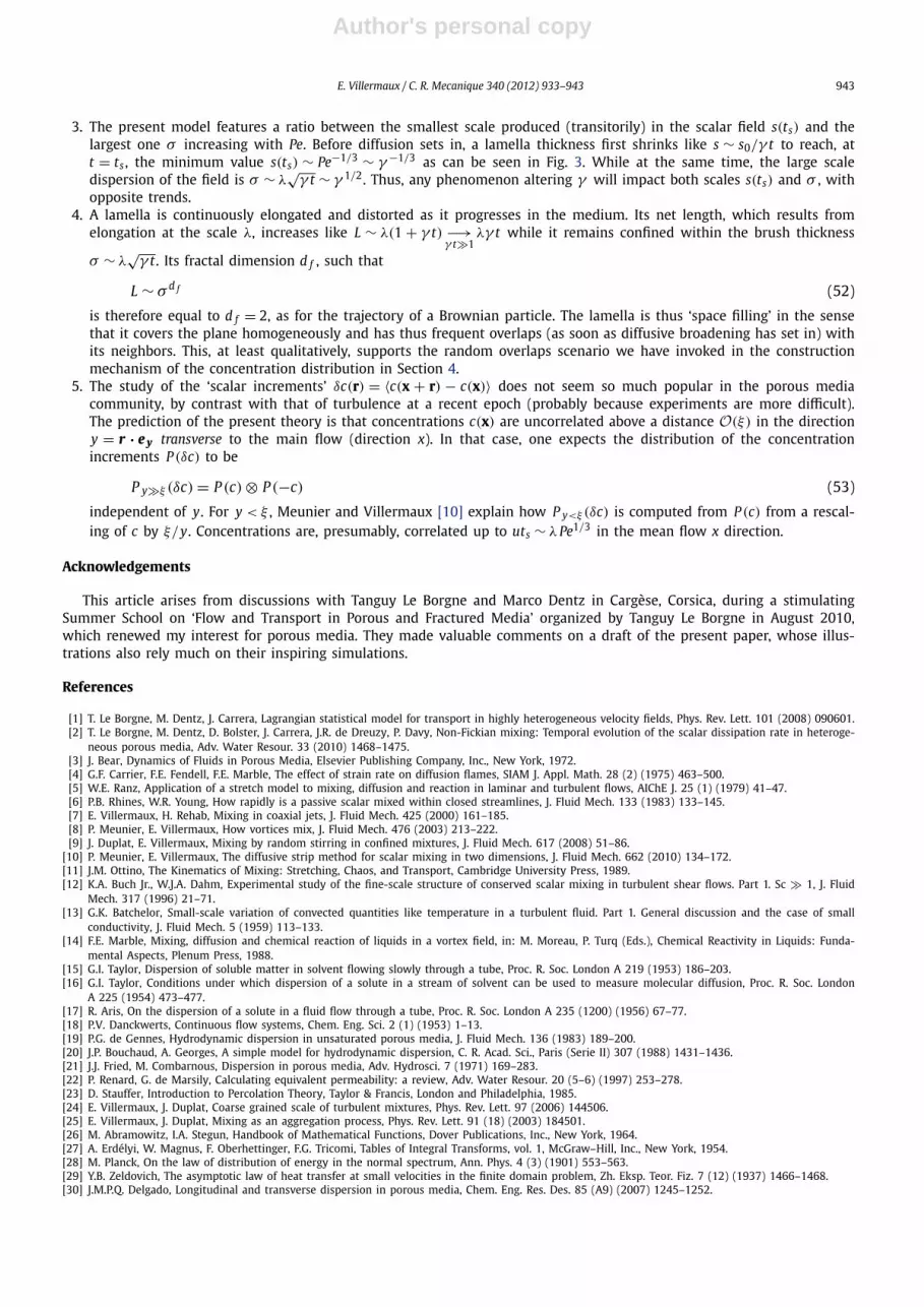
Fig. 6. The distribution of the number of quanta q(n) given in (33), corresponding to the spatial profile of n displayed in the insert according to (31) withn0 = 100.

The average number of overlaps which, by addition (the diffusive profiles of adjacent lamella add, owing to the linearity ofthe Fourier equation3) restore the average concentration must thus be

〈n〉 = 〈C〉θ

∼ γ t√Pe

(26)

One can be more precise, and compute from this representation the overall concentration distribution of the mixture.

4.1. The elementary strips as quanta

We conduct the discussion in the concentration distribution space, and consider an elementary strip as a quantum,interacting with its neighbors according to a precise rule to form the macroscopic field, that is:

1. Quanta: The elementary lamellae, or strips formed by the random advection, each of them bearing an average concen-tration θ , solely function of time. The elementary strip is the indivisible brick of the mixture;

2. Macroscopic ensemble: The average spatial concentration field C(x, t), and its concentration distribution P (c). The en-semble average of c at a location x defines the mean envelope, namely 〈c〉x = C(x, t);

3. Composition rule: Random overlap of the lamellae and addition of the concentration levels (quanta) θ , restoring C(x, t)on average, and thus building P (c).

If locally in the medium the value a concentration level c is the result of the addition of n individual contributions, comingfrom n different lamella, and if these contributions are made at random, that is if the merged lamellae have had differ-ent, uncorrelated past histories in the medium (an assumption which could be checked from numerical simulations), thengeneral principles (see [25,9]) suggest that the concentration distribution itself will be given by

p(c|n) = 1

Γ (n)

(c

θ

)n−1 e− cθ

θ(27)

which is conveniently written in Laplace transform

p(s|n) =∞∫

0

e−sc p(c|n)dc (28)

as

p(s|n) = (1 + sθ)−n (29)

The moments of p(c|n) are such that 〈ck〉 = (−1)k[∂ks p(s|n)]s=0. In particular, the mean concentration carried by a bundle

of n aggregated lamellae is 〈c〉 = nθ . Note that a very large number of random additions leads to a uniform concentrationsince

3 For instance, on a still (u = 0 in (2)) d-dimensional substrate, the concentration field θ(r, t) results from the additive contribution of the initial

concentration spatial distribution through the Green function θ(r, t) = (4π Dt)−d/2∫

exp[−(r − r′)2/4Dt]θ(r′,0)dr′.



p(c|n → ∞) → δ(c − nθ) (30)

However, the number n depends on the position x along the bundle (in a frame moving at the average speed u) since itsets the number of overlaps which, locally, restore C(x, t) from θ . This number is therefore spatially distributed accordingto n = C(x, t)/θ , or (Fig. 6)

n = n0e− x2

2σ2 with n0 = s0

σθ∼ γ t√

Pe(31)

Let q(n) be the probability density to find a given value of n in the field; this value is a continuous variable since it derivesfrom a mean smooth spatial profile (31), but it cannot, however, take values below 1 since a single elementary lamellacarries the smallest concentration increment in the field, namely θ . Obviously, the overall concentration distribution P (c)will be

P (c) =n0∫

1

p(c|n)q(n)dn (32)

To the spatial profile of n (which directly reflects that of C(x, t)) is associated the probability q(n) as

q(n) ∼ 1

σ �n�x

∼ 1

n√

ln(n0/n)(33)

with a normalizing constant (2√

ln n0)−1. The distribution q(n) is indeed normalized when the integral is restricted to the

population of quanta, i.e. for n = 1 to n0, as in (32). It has the characteristic U-shape of the probability density associated toa spatial Gaussian profile [8]. The small-n behavior is

q(n) ∼ 1

nfor n � n0 (34)

while for n close to n0, the distribution has a singularity

q(n) → δ(n − n0) (35)

Thus, the low concentration side (i.e. for c < n0θ , but still c > θ , and thus s θ < 1) of the global P (c) can be obtained from(32) by letting the integral run up to infinity; in Laplace space (32) writes

P (s) ≈∞∫

1

(1 + sθ)−n

ndn = Γ

(0, ln(1 + sθ)

)(36)

so that, since Γ (0, ε)−→ε→0

−0.577 − lnε + ε +O(ε2) (see [26])

P (s) ≈ ln

(1 + sθ

sθ

)(37)

and thus the low concentration side of the overall distribution is, [27]:

P (c) ≈ 1 − e− cθ

c→ 1

cfor θ < c < n0θ (38)

corresponding to the exploration of the tails of the spatial mean profile n in (31). The largest concentrations are found closeto the center of the bundle, where the maximum of additions occurs (of the order of n0). There, owing to (27) and (35),one expects P (s) ≈ p(s|n0) = (1 + s θ)−n0 , that is

P (c) ≈ p(c|n0) → e− cθ for c � n0θ (39)

The overall shape of P (c) is shown in Fig. 7.

4.2. The necessity for quanta

Although the two estimates coincide at low concentration (i.e. P (c) ∼ 1/c), the distribution P (c) does not derive fromthe average smooth spatial concentration profile C(x, t); in other words, the statistics of the field is not the statistics of themean field

P (c) = 1

σ �C�x |C=c

(40)



Fig. 7. Left: The distribution of concentration resulting from the random aggregation of n lamellae given in (27), with n = 10. Right: The concentrationdistribution P (c) in the bundle given in (32) for n0 = 100.

Fig. 8. Left: A lamellae broadening by pure diffusion in a quiescent environment. Right: Mixing in the ‘brush’ in the presence advection in a heterogeneousporous medium (adapted from Le Borgne et al. [2]).

If it were, P (c) would present the same singular U-shape as q(n) does, with the same logarithmic divergence at the maximalconcentration c = C(0, t), which is unphysical. The quantum construction of the distribution in (32) removes this singularity.It is the distribution of the number of quanta q(n) which is singular in n = n0 (much more singular than p(s|n) which is abroad decaying exponential in n for sθ → 0, i.e. (1 + sθ)−n); therefore the integral in (32) equals to p(s|n = n0) correspond-ing, in concentration space c, to a Gamma distribution with a regularized smooth exponential fall off e−c/θ .

As for Planck’s construction of the blackbody radiation law [28], the distribution P (c) is tangent to the continuous (clas-sical) distribution at low concentration (energy), but its discrete nature has regularized the artifact of a flawed continuousdescription at high concentration (energy), by removing the inappropriate divergence (ultraviolet catastrophe).

5. Scalar dissipation

The ‘scalar dissipation’, or ‘rate of dissipation’ χ was introduced in the theory of turbulence (Zeldovich [29]) since itbridges a small scale feature of the mixture (the concentration gradients) with the global decay rate of the concentrationfluctuations c. In an impermeable system with the mean 〈c〉 conserved,

χ = −∂t⟨c2⟩ = 2D

⟨(∇c)2⟩ (41)

For instance, a lamellae diluting in a wide quiescent substrate by pure diffusion (Fig. 8) has a dissipation rate given by

χ ∼√

s20/D

t3/2(42)

since for t > s20/D , one has from the corresponding one-dimensional diffusion problem

c(x, t) ∼ s0

2√

π Dte− x2

4Dt (43)

the following estimates

(∇c)2 =O(c(0, t)2/s2) with c(0, t) ∼ s0/

√Dt and s ∼ √

Dt (44)

and also remembering that the spatial average in (41) involves the ratio of the relative lamella surface area s/s0.Considering a line initially perpendicular to the mean flow in a porous medium, dissipation occurs within the ‘brush’

whose width σ ∼ λ√

γ t increases in time, realizing an open system with an average concentration decaying in time. Thebrush has a mean rate of expansion (σ /σ ), over which incompressible velocity fluctuations are superimposed so thatthe corresponding convection diffusion problem becomes in a reference frame traveling at the mean drift velocity u (seeSection 3.1) in the x direction



⎧⎪⎨⎪⎩

∂tc + ∇ · (u c) = D∇2c

u = x(σ /σ )ex + v∇ · v = 0

(45)

The brush expands by incorporating diluting fluid at its frontiers in x = ±σ/2 so that c(x = ±σ/2, t) = 0, and therefore, onegets from (45) the evolution of the mean squared concentration generalized to an open system as⟨

∂tc2⟩ + (σ /σ )⟨c2⟩ = −2D

⟨(∇c)2⟩ (46)

The additional term in (46) compared to (41) is trivially due to the decay of the average concentration since indeed σ /σ =−∂t〈C〉/〈C〉. The dissipation rate χ = −〈∂tc2〉 is readily computed by noting that, for t > ts = γ −1 Pe1/3

(∇c)2 =O(θ2/s2) with θ ∼ (t/ts)

−3/2 and s ∼ √Dt (47)

and that the spatial average in (46) involves the ratio of the lamella surface λγ t√

Dt to that of the domain λσ = λ2√γ t .Both the dilution term (σ /σ )〈c2〉, and the molecular diffusion term 2D〈(∇c)2〉 have the same scaling, which is

χ ∼√

Pe

γ 2t3(48)

a trend which does not seem inconsistent with the numerics of Le Borgne et al. [2] at large times (when the initial straightline geometry has been sufficiently distorted by the flow, i.e. for γ t > 1, the short time limit is described by (42)), and forstrongly heterogeneous media (for which the stretched lamella representation has a chance to be relevant). Note that thetime dependence obtained by Meunier and Villermaux [8] in a similar problem is slightly different since these authors wereintegrating (and not averaging) χ over a time dependent support (a developing spiral).

The dissipation rate χ is a quantity which is sometimes modeled ab initio for closure purposes, and it has been derivedabove in the traditional way. In fact, we already knew it. It is a consequence of our theory, rather than a building ingredient.We have this information from the overall distribution P (c) and its time evolution, which we have inferred without resortingto a particular model for χ , but rather from detailed microscopic diffusion and a general principle of random superposition.We have

χ = −∂t(⟨

c2⟩ − 〈c〉2) (49)

with 〈c〉 = −[∂s P (s)]s=0 and 〈c2〉 = [∂2s P (s)]s=0 and from (32)

P (s) =n0∫

1

(1 + sθ)−nq(n)dn (50)

The dissipation is controlled by the large concentration gradients, which themselves occur where the concentration is large.Therefore, the appropriate limit for q(n) is (35), giving P (s) ≈ (1 + sθ)−n0 , and thus

χ = −∂t(n0θ

2) (51)

which, with n0 ∼ γ t/√

Pe and θ ∼ (γ t/Pe1/3)−3/2, gives (48) in a straightforward way.

6. Concluding remarks

We have proposed a simple, unified framework to understand the fine structure of a scalar mixture progressing in arandom, interconnected but rigid network of paths, namely a porous medium. We have described the relevant scales ofthe mixture, the kinetics of their evolution, the nature of their interaction, and the scaling laws describing the coarseningprocess of the concentration field as it progresses through the medium, including the shape and deformation of the concen-tration distribution from a line source, at any time. A few remaining remarks are in order; some of them could be testedexperimentally, or from numerical simulations in the spirit of those by Le Borgne et al. [2]:

1. Our analysis does not exhibit any ‘anomaly’ in the sense that dispersion and convection diffusion problems treatedhere all rely on the traditional physics of diffusion from Gauss and Fourier, even if its implementation on a deformingsubstrate (what happens at the scale of the velocity correlation length λ, see Section 3.2) leads to ‘non-square root’scaling laws. A possible difference with actual porous media, in particular regarding large scale dispersion (i.e. thestatus of σ ), may be attributed to transients and crossovers between the ballistic, and pure ‘square root’ dispersion. Thecrossover is all the more long that the medium is heterogeneous (Le Borgne et al. [2]).

2. We were interested in a line source initially materialized perpendicular to the flow average direction. The case of a pointsource would lead to the same results, except that the transverse percolation problem would not produce a percolationcluster wider than the large scale transverse dispersion width σ⊥ , itself proportional but smaller in amplitude (Delgado[30]), to the longitudinal dispersion σ .



3. The present model features a ratio between the smallest scale produced (transitorily) in the scalar field s(ts) and thelargest one σ increasing with Pe. Before diffusion sets in, a lamella thickness first shrinks like s ∼ s0/γ t to reach, att = ts , the minimum value s(ts) ∼ Pe−1/3 ∼ γ −1/3 as can be seen in Fig. 3. While at the same time, the large scaledispersion of the field is σ ∼ λ

√γ t ∼ γ 1/2. Thus, any phenomenon altering γ will impact both scales s(ts) and σ , with

opposite trends.4. A lamella is continuously elongated and distorted as it progresses in the medium. Its net length, which results from

elongation at the scale λ, increases like L ∼ λ(1 + γ t) −→γ t�1

λγ t while it remains confined within the brush thickness

σ ∼ λ√

γ t . Its fractal dimension d f , such that

L ∼ σ d f (52)

is therefore equal to d f = 2, as for the trajectory of a Brownian particle. The lamella is thus ‘space filling’ in the sensethat it covers the plane homogeneously and has thus frequent overlaps (as soon as diffusive broadening has set in) withits neighbors. This, at least qualitatively, supports the random overlaps scenario we have invoked in the constructionmechanism of the concentration distribution in Section 4.

5. The study of the ‘scalar increments’ δc(r) = 〈c(x + r) − c(x)〉 does not seem so much popular in the porous mediacommunity, by contrast with that of turbulence at a recent epoch (probably because experiments are more difficult).The prediction of the present theory is that concentrations c(x) are uncorrelated above a distance O(ξ) in the directiony = r · e y transverse to the main flow (direction x). In that case, one expects the distribution of the concentrationincrements P (δc) to be

P y�ξ (δc) = P (c) ⊗ P (−c) (53)

independent of y. For y < ξ , Meunier and Villermaux [10] explain how P y<ξ (δc) is computed from P (c) from a rescal-ing of c by ξ/y. Concentrations are, presumably, correlated up to uts ∼ λPe1/3 in the mean flow x direction.

Acknowledgements

This article arises from discussions with Tanguy Le Borgne and Marco Dentz in Cargèse, Corsica, during a stimulatingSummer School on ‘Flow and Transport in Porous and Fractured Media’ organized by Tanguy Le Borgne in August 2010,which renewed my interest for porous media. They made valuable comments on a draft of the present paper, whose illus-trations also rely much on their inspiring simulations.

References

[1] T. Le Borgne, M. Dentz, J. Carrera, Lagrangian statistical model for transport in highly heterogeneous velocity fields, Phys. Rev. Lett. 101 (2008) 090601.[2] T. Le Borgne, M. Dentz, D. Bolster, J. Carrera, J.R. de Dreuzy, P. Davy, Non-Fickian mixing: Temporal evolution of the scalar dissipation rate in heteroge-

neous porous media, Adv. Water Resour. 33 (2010) 1468–1475.[3] J. Bear, Dynamics of Fluids in Porous Media, Elsevier Publishing Company, Inc., New York, 1972.[4] G.F. Carrier, F.E. Fendell, F.E. Marble, The effect of strain rate on diffusion flames, SIAM J. Appl. Math. 28 (2) (1975) 463–500.[5] W.E. Ranz, Application of a stretch model to mixing, diffusion and reaction in laminar and turbulent flows, AIChE J. 25 (1) (1979) 41–47.[6] P.B. Rhines, W.R. Young, How rapidly is a passive scalar mixed within closed streamlines, J. Fluid Mech. 133 (1983) 133–145.[7] E. Villermaux, H. Rehab, Mixing in coaxial jets, J. Fluid Mech. 425 (2000) 161–185.[8] P. Meunier, E. Villermaux, How vortices mix, J. Fluid Mech. 476 (2003) 213–222.[9] J. Duplat, E. Villermaux, Mixing by random stirring in confined mixtures, J. Fluid Mech. 617 (2008) 51–86.

[10] P. Meunier, E. Villermaux, The diffusive strip method for scalar mixing in two dimensions, J. Fluid Mech. 662 (2010) 134–172.[11] J.M. Ottino, The Kinematics of Mixing: Stretching, Chaos, and Transport, Cambridge University Press, 1989.[12] K.A. Buch Jr., W.J.A. Dahm, Experimental study of the fine-scale structure of conserved scalar mixing in turbulent shear flows. Part 1. Sc � 1, J. Fluid

Mech. 317 (1996) 21–71.[13] G.K. Batchelor, Small-scale variation of convected quantities like temperature in a turbulent fluid. Part 1. General discussion and the case of small

conductivity, J. Fluid Mech. 5 (1959) 113–133.[14] F.E. Marble, Mixing, diffusion and chemical reaction of liquids in a vortex field, in: M. Moreau, P. Turq (Eds.), Chemical Reactivity in Liquids: Funda-

mental Aspects, Plenum Press, 1988.[15] G.I. Taylor, Dispersion of soluble matter in solvent flowing slowly through a tube, Proc. R. Soc. London A 219 (1953) 186–203.[16] G.I. Taylor, Conditions under which dispersion of a solute in a stream of solvent can be used to measure molecular diffusion, Proc. R. Soc. London

A 225 (1954) 473–477.[17] R. Aris, On the dispersion of a solute in a fluid flow through a tube, Proc. R. Soc. London A 235 (1200) (1956) 67–77.[18] P.V. Danckwerts, Continuous flow systems, Chem. Eng. Sci. 2 (1) (1953) 1–13.[19] P.G. de Gennes, Hydrodynamic dispersion in unsaturated porous media, J. Fluid Mech. 136 (1983) 189–200.[20] J.P. Bouchaud, A. Georges, A simple model for hydrodynamic dispersion, C. R. Acad. Sci., Paris (Serie II) 307 (1988) 1431–1436.[21] J.J. Fried, M. Combarnous, Dispersion in porous media, Adv. Hydrosci. 7 (1971) 169–283.[22] P. Renard, G. de Marsily, Calculating equivalent permeability: a review, Adv. Water Resour. 20 (5–6) (1997) 253–278.[23] D. Stauffer, Introduction to Percolation Theory, Taylor & Francis, London and Philadelphia, 1985.[24] E. Villermaux, J. Duplat, Coarse grained scale of turbulent mixtures, Phys. Rev. Lett. 97 (2006) 144506.[25] E. Villermaux, J. Duplat, Mixing as an aggregation process, Phys. Rev. Lett. 91 (18) (2003) 184501.[26] M. Abramowitz, I.A. Stegun, Handbook of Mathematical Functions, Dover Publications, Inc., New York, 1964.[27] A. Erdélyi, W. Magnus, F. Oberhettinger, F.G. Tricomi, Tables of Integral Transforms, vol. 1, McGraw–Hill, Inc., New York, 1954.[28] M. Planck, On the law of distribution of energy in the normal spectrum, Ann. Phys. 4 (3) (1901) 553–563.[29] Y.B. Zeldovich, The asymptotic law of heat transfer at small velocities in the finite domain problem, Zh. Eksp. Teor. Fiz. 7 (12) (1937) 1466–1468.[30] J.M.P.Q. Delgado, Longitudinal and transverse dispersion in porous media, Chem. Eng. Res. Des. 85 (A9) (2007) 1245–1252.

Documents

Mixing by porous media