MIP: THEORY AND PRACTICE CLOSING THE GAP - Springer

The original version of this chapter was revised: The copyright line was incorrect. This has beencorrected. The Erratum to this chapter is available at DOI: 10.1007/978-0-387-35514-6_15

MIP: THEORY AND PRACTICE CLOSING THE GAP

Robert E. Bixby !LOG CPLEX Division

889 Alder Avenue

Incline Village, NV 89451, USA

and

Department of Computational and Applied Mathematics

Rice University

Houston, TX 77005-1892, USA

bibxylikaam.rice.edu

Mary Fenelon !LOG CPLEX Division

889 Alder A venue

Incline Village, NV 89451, USA

Zonghao Gu As above

Ed Rothberg As above

Roland Wunderling As above

1. INTRODUCTION For many years the principal solution technique used in the practice

of mixed-integer programming has remained largely unchanged: Linear programming based branch-and-bound, introduced by Land and Doig (1960). This, in spite of the fact that there has been significant progress

M.J.D. Powell and S. Scholtes (Eds.), System Modelling and Optimization: Methods, Theory and Applications. © 2000 IFIP International Federation for Information Processing. Published by Kluwer Academic Publishers. All rights reserved.

http://dx.doi.org/10.1007/978-0-387-35514-6_15

20 R.E. Bixby, M. Fenelon, Z. Cu, E. Rothberg and R. Wunderling

in the theory of integer programming and in the closely related field of combinatorial optimization. Many of the ideas developed there have received extensive computational testing, but, until recently, relatively little of that work has made it into the commercial codes used by practitioners. That situation has now changed. Several such codes, among them LING0 1, OSL2, and XPRESS-Mp3 , as weIl as the CPLEX4 code studied in this paper, now include cutting-plane capabilities as weIl as other ideas from the backlog of accumulated theory. As suggested by the title of this paper, the gap between theory and practice is indeed closing.

In order to fix ideas, we begin with a formal definition. A mixedinteger program (MIP) is an optimization problem of the form

mmlmlze cTx

subject to Ax = b l:;'x:;'u

some or all Xj integral,

where A is an mX n matrix, caIled the constraint matrix, xis a vector of variables, c is the objective junction, and land u are vectors of bounds. Thus, a MIP is a linear program (LP) plus an integrality rest riet ion on some or aIl of the variables. This last restrietion is what makes MIPs diffieult (NP-hard, in the teehnical sense); it takes a weIl understood, convex problem and makes it non-convex. It also makes the mixedinteger modeling paradigm a powerful tool in representing real-world business applications.

The power of the mixed-integer modeling paradigm was recognized almost immediately, dating back to the 50s and 60s, and numerous attempts were made to apply it. Unfortunately, while the modeling paradigm was strong, the available software and computers for solving the models were not. The result was disillusionment, so me of which persists to this day. Many potential practitioners still believe that mixedinteger programming is nice to talk about, but has limited practical applieability. An important message of this paper is that this situation has changed, and changed dramatically just in the last year. It is now possible to solve many difficult, interesting, and practical mixed-integer models using off-the-shelf software.

The following is an outline of the contents of the paper. We begin with a discussion of advances in methods for solving linear programming

1 LINGO is a trademark of Lindo Systems, Ine. 20SL is a trademark of IBM Corporation 3XPRESS-MP is a trademark Dash Assoeiates Ltd. 4CPLEX is a trademark of ILOG, Ine.

MIP: The01'Y and Practice - Closing the Gap 21

problems. First we give a snapshot overview of developments in the period from the mid-80s to 1998, and then we look at 1999. One reason to begin with linear programming, rather than directly with mixed-integer programming, is that linear programming is an enabling technology for solving MIPs. Given this first reason, the real motivation for including a discussion of linear programming here is that 1999 has seen some remarkable and unexpected improvements in the classical simplex method.

The discussion of linear programming will be followed by the mixedinteger programming part of the paper. The presentation emphasizes features. Specific topics to be discussed will include node presolve, heuristics for finding feasible solutions, and cutting planes. These will be followed by extensive computational results.

The discussion of mixed-integer programming features can be viewed as having two main parts. The first discusses features that attempt to decrease the "upper bound" (e.g., heuristics to find better integral solutions). The second discusses features that attempt to increase the lower bound (e.g., cutting planes). When the upper and lower bounds become equal, the computation is finished.

An important guiding principle of our mixed-integer algorithmic developments is that solving MIPs often requires a "barrage" of different, but cooperating ideas. In other words, we try to take advantage of structures that are common to many real-world MIPs, hoping that some or all will contribute to a better solution for a particular model. To do so, it is essential to develop good defaults, and implement the individual ideas in such a way that they help when they can, and otherwise hurt as little as possible. This approach is perhaps different from that of most theoretical investigations, where the goal is typically to demonstrate the efficacy of a particular new idea, usually in isolation.

Finally, we consider several examples. Two of these examples will provide a counter balance to the idea that good defaults are sufficient to handle all models. While we would like to run mixed-integer programming codes much as we run linear-programming codes, as black boxes, there will always be instances that demand some sort of tuning or reformulation.

We close this section with one general re mark. For many of the computational results presented in this paper, we will use geometric means as a method to summarize results. On occasion, when doing so, we will simply use the word "mean." This usage will always refer to the geometric mean, and not the more common arithmetic mean. Arithmetic means can be quite misleading when applied to a set of ratios, as would often be the case in this paper.

22 R.E. Bixby, M. Fenelon, Z. Gu, E. Rothberg and R. Wunderling

2. LINEAR PROGRAMMING 2.1. PROGRESS SOLVING LPS: MID-80S TO

1998

No attempt is made he re to discuss linear-programming improvements in this period in detail. We will present just one table, followed by a brief discussion. A detailed discussion is a topic unto itself.

As the following table illustrates, over the past ten years there has been steady progress in our ability to solve linear programming problems5 .

Model: PDS-30, Patient Distribution System 49944 rows, 177628 columns, 393657 nonzeros

Version

CPLEX 1.0 (1988) CPLEX 3.0 (1994) CPLEX 5.0 (1996)

Time (seconds)

57840 4555 3835

The model PDS-30 is one of a cIass of models introduced in Carolan, et al., (1990), and is well-known within the linear-programming community. For reasons that are hopefully apparent given the CPLEX 1.0 data in the table, the larger instances in this dass (e.g., PDS-30) were considered very difficult when first introduced. The runtimes in the table were produced using a modern workstation, a 296 MHz Sun UltraSparc. Considering the improvement in machine speeds between 1990 and the present, probably exceeding a multiple of 1,000, describing this model as being very difficult in 1990 is an understatement.

Some remarks are in order before we move on to the developments of the last year. First, while it is not illustrated in this table, the first release of CPLEX was already a significant improvement over at least one of the standard portable codes available at that time, XMP developed by Marsten (1981). Thus, the fifteen-fold improvement for the one problem in the table in the period 1988 to 1998 can be viewed as an underestimate. Second, and much more important in our view, the most significant development of the last decade is not really reflected in this

5In CPLEX 1.0 only a primal simplex algorithm was available. In subsequent versions, primal and dual simplex algorithms, and a barrier algorithm were available. We used the dual simplex algorithm when solving PDS-30 with CPLEX 3.0 and 5.0.

MIP: Theory and Practice - Closing the Gap 23

table. This development was the leap forward in robustness of linear programming codes. They have not only become more robust in terms of salve times, but also much more robust at handling numerical difficulties and problems related to degeneracy. In short, linear programming has become more-and-more a tool that practitioners can simply use, embedding it as a black box in other applications without having to worry whether it will do its job.

2.2. PROGRESS SOLVING LPS: 1999 We began the work described in this seetion by making a simple ob

servation: LPs have become larger. This is the same sort of observation that was made ten years aga at the start of the developments highlighted in the previous section. Here it led us to focus specifically on models with at least 10,000 constraints. It also led us to focus on the simplex method, since it was the simplex method that seemed to be underperforming on these large models. It didn't take long to discover where the bottleneck lay: The solution of the two (sometimes three) linear systems that are necessary at each simplex iteration. These linear systems are commonly called BTRAN and FTRAN (see Chvatal (1983)).

It is not strictly necessary to know what the FTRAN and BTRAN systems refer to here. The basic idea is quite simple. Imagine we are to solve a large linear system Lx = a, where L is a triangular matrix, a is extremely sparse, and x turns out to be very sparse as weIl. Both vectors often have fewer than 100 nonzeros among them, in spite of the fact that L is of order 10,000 or more (corresponding to a linear programming problem with 10,000 or more constraints). Clearly, when a and x contain this few nonzeros, it is unlikely that the cause was cancellation during the solve; more likely is that the number of nonzeros touched in L, in order to compute x, was very small as weIl. Thus, the key to reducing the cost of the solve is to do it in an amount of time linear in this number of nonzeros. As it turns out, though this fact was apparently not being exploited in linear programming codes, the existence of such an algorithm has long been known in the sparse linear algebra community. It is equivalent to a certain, natural reachability problem in a graph. See Gilbert and Peierls (1988).

When the above bottleneck was removed, it then made possible further improvements to the simplex method itself. This is where the r·eal progress occurred. Two examples:

• The dual simplex algorithm: It can be shown that variables with two finite bounds often do not need to be binding in the ratio


test. Exploiting that fact leads to what one might call a "longstep" dual simplex algorithm.

• Fast pricing update: If the solutions of the key linear systems at each iteration are sparse, then it is reasonable to expect that only a small number of reduced costs will change, and hence that appropriate update schemes can be introduced to accelerate the choices of entering and leaving variables in the primal and dual simplex algorithms, respectively.

For PDS-30, the resulting improvement is significant indeed:

Model: PDS-30, Patient Distribution System 49944 rows, 177628 columns, 393657 nonzeros

Version

CPLEX 1.0 (1988) CPLEX 3.0 (1994) CPLEX 5.0 (1996) CPLEX 6.5 (1999)

Time (seconds)

57840 4555 3835

165

Of course, PDS-30 is just one problem, used here as an illustration. Much more extensive tests were done to evaluate the effects of the changes introduced with CPLEX 6.5. In addition to the changes outlined above for the simplex method, there were also important, if not quite as dramatic, improvements in the barrier implementations. These barrier improvements can be summarized as due to two things: (a) Better ordering algorithms for the computation of the Cholesky factorization, see Rothberg and Hendrickson (1998), and (b) better exploitation of the available level-two cache in modern computing architectures, see Rothberg and Gupta (1991).

In what follows, an extensive set of test results are given to evaluate the performance improvements in CPLEX 6.5. The results are broken into two parts: Small models and large models. Before plunging into the details, it is perhaps worthwhile to point out the philosophy of the way the improvements were implemented. The overall target was "robustness and scalability" in the algorithms. At least as important as making the algorithms better on larger models was that performance did not degrade, and hopefully improved, on the broad middle-range of models that dominate in practice. Indeed, while the improvements on large models were exciting and were the impetus behind this work, the real


effort was expended in making sure that these improvements didn't get in the way when they didn't help. The same theme was mentioned earlier for mixed-integer programming.

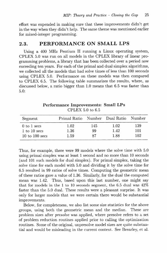
2.3. PERFORMANCE ON SMALL LPS Using a 400 MHz Pentium II running a Linux operating system,

CPLEX 5.0 was run on all models in the CPLEX library of linear programming problems, a library that has been collected over aperiod now exceeding ten years. For each of the primal and dual simplex algorithms, we collected all the models that had solve times of less than 100 seconds using CPLEX 5.0. Performance on these models was then compared to CPLEX 6.5. The following table summarizes the results, where, as discussed below, a ratio bigger than 1.0 means that 6.5 was faster than 5.0:

Performance Improvements: Small LPs CPLEX 5.0 to 6.5

Segment Primal Ratio Number Dual Ratio Number

o to 1 secs 1.02 145 1.02 139 1 to 10 secs 1.36 99 1.42 101 10 to 100 secs 1.59 87 1.88 102

Thus, for example, there were 99 models where the solve time with 5.0 using primal simplex was at least 1 second and no more than 10 secemds (and 101 such models for dual simplex). For primal simplex, taking the solve time for each model with 5.0 and dividing it by the solve time for 6.5 resulted in 99 ratios of solve times. Computing the geometric mean of these ratios gave a value of 1.36. Similarly, for the dual the computed mean was 1.42. Thus, based upon this last number, one might say that for models in the 1 to 10 seconds segment, the 6.5 dual was 42% faster than the 5.0 dual. These results were a pleasant surprise. It was only for larger models that we were certain there would be substantial improvements.

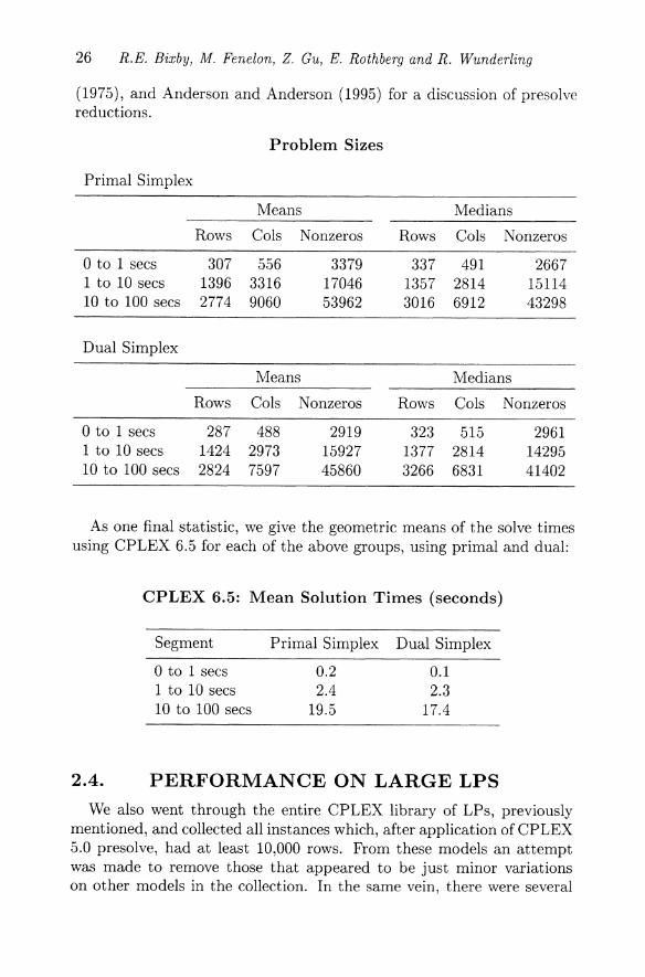
Below, for completeness, we also list so me size statistics for the above groups, using both the geometrie me an and the median. These are problem sizes after presolve was applied, where presolve refers to CL set of problem reduction routines applied prior to calling the optimization routines. Some of the original, unpresolve model sizes are quite substantial and would be misleading in the current context. See Brearley, et al.


(1975), and Anderson and Anderson (1995) for a diseussion of presolve reduetions.

Problem Sizes

Primal Simplex

Means Medians

Rows Cols Nonzeros Rows Cols Nonzeros

o to 1 sees 307 556 3379 337 491 2667 1 to 10 sees 1396 3316 17046 1357 2814 15114 10 to 100 sees 2774 9060 53962 3016 6912 43298

Dual Simplex

Means Medians

Rows Cols Nonzeros Rows Cols Nonzeros

o to 1 sees 287 488 2919 323 515 2961 1 to 10 sees 1424 2973 15927 1377 2814 14295 10 to 100 sees 2824 7597 45860 3266 6831 41402

As one final statistie, we give the geometrie means of the solve times using CPLEX 6.5 for eaeh of the above groups, using primal and dual:

CPLEX 6.5: Mean Solution Times (seconds)

Segment Primal Simplex Dual Simplex

o to 1 sees 0.2 0.1 1 to 10 sees 2.4 2.3 10 to 100 sees 19.5 17.4

2.4. PERFORMANCE ON LARGE LPS We also went through the entire CPLEX library of LPs, previously

mentioned, and eollected all instanees whieh, after applieation of CPLEX 5.0 presolve, had at least 10,000 rows. From these models an attempt was made to remove those that appeared to be just minor variations on other models in the eolleetion. In the same vein, there were several


instances, such as the PDS models, where a whole family of models with increasing sizes were found. In these cases, the largest instance from the family was included in the test-set and the others deleted.

All runs were done on PCs with 400 MHz Pentium II processors running a Linux operating system. Models were included in the final performance numbers only if, in presolved form, they were solvable wit.hin one-half Gigabyte of physical memory. This limitation was dictated by memory availability on our test machines. A time limit of 500,000 seconds (about 6 days) was also imposed for each run. A limit this large may seem excessive, but it was deemed necessary for the tests since the expectation was that several models would solve in several thousands of seconds with CPLEX 6.5 and would be a large multiple slower with CPLEX 5.0. Comparisons would not have been possible otherwise. Note that in the final analysis of the data, where ratios are used to compare the various algorithms, models that exceeded the memory limit were not included. However, those that reached the time limit were included, in such cases using 500,000 seconds as the run time. As a result the comparisons we made underestimated the actual improvements.

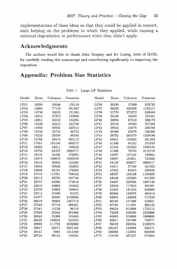
Table 1 in the appendix gives size statistics for the models generated, ordered by the number of constraints in the model. Generic names (LP01 through LP90, ordered by increasing numbers of constraints) have been used since many of these models are proprietary. The mean number of constraints was about 50,000, with three models having over 1,000,000 constraints. The following two tables summarize comparötive performance as problem size grows. There are distinct tables for barrier and simplex (plus best) since the sets of models not meeting the memory restriction were different.

Performance Improvements: Large LPs CPLEX 5.0 to 6.5

Mean Ratios

Problems Primal Simplex Dual Simplex Best

Biggest 10 8.5 22.3 18.0 Biggest 20 7.9 18.8 12.2 Biggest 30 7.4 20.2 11.3 Biggest 40 6.4 14.0 8.0 Biggest 50 5.5 11.9 6.7 Biggest 60 5.2 10.1 6.2 Biggest 70 5.1 9.1 5.6 Biggest 80 4.5 8.2 5.2 All 4.4 8.0 5.2


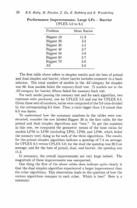
Performance Improvements: Large LPs - Barrier CPLEX 5.0 to 6.5

Problem

Biggest 10 Biggest 20 Biggest 30 Biggest 40 Biggest 50 Biggest 60 Biggest 70 All

Mean Ratios

11.9 5.5 4.1 3.7 3.6 3.7 3.6 3.6

The first table above refers to simplex results and the best of primal and dual simplex and barrier, where barrier includes crossover to abasie solution. The total number of models in the All category for simplex was 86; four models failed the memory-limit test. 75 models are in the All category for barrier; fifteen failed the memory-limit test.

For each model passing the memory test and for each algorithm, two runtimes were produced, one for CPLEX 5.0 and one for CPLEX 6.5. Given these sets of numbers, ratios were computed of the 5.0 time divided by the corresponding 6.5 time. Thus, a ratio bigger than 1.0 meant that 6.5 was faster.

To understand how the summary numbers in the tables were constructed, consider the row labeled Biggest 30 in the first table, for the primal and dual simplex algorithms and "best." To get the numbers in this row, we computed the geometrie means of the time ratios for models LP58 to LP90 (excluding LP85, LP89, and LP90, which failed the memory test) doing so for each of the three algorithms. The results for the primal simplex algorithm indicate a speedup of 7.4 on average, for CPLEX 6.5 versus CPLEX 5.0; for the dual the speedup was 20.2 on average; and for the best of primal, dual, and barrier, the speedup was 11.3.

In summary, the overall improvements are very large indeed. The magnitude of these improvements was unexpected.

One thing the first of the above tables does indicate quite clearly is that the dual simplex algorithm experienced a larger improvement than the other algorithms. This observation leads to the quest ion of how the various algorithms compare to each other. Which is best? Here is a summary:


CPLEX 6.5: Algorithm Comparison

Algorithms Instances Mean Wins for Dual

Primal/Dual 86 2.6 56 Barrier /Dual 78 1.2 41

Thus, dividing the primal solve time for each model by the dual salve time and computing the geometrie means of the resulting ratios gives the result that the dual was a factor of 2.6 faster overall. 86 models were ineluded in the test. In 56 of the instances dual was the winner. In 30 instances primal won. For the barrier versus dual comparison, it was much eloser, with dual winning by only a small margin, but winning nevertheless, with a mean ratio of 1.2. Dual was the faster algorithm in 41 instances, while barrier won in 37 instances.

Missing from the table, because of the focus on the dual, is the comparison between barrier and primal. In that comparison barrier won 46 times and primal 32 times, and the mean ratio was 1.8, with barrier the winner. Finally, doing a comparison among all algorithms, using all 90 models (see Remark 3, below), we obtain the interesting result that primal won 18 times, dual 33 times, and barrier 39 times.

Remarks:

1 Among the 86 instances in which CPLEX 6.5 primal and dual were compared, primal and dual reached the 500,000 second time limit on one common model. This model contributed a 1.0 to the mean ratio. There were six additional instances in which the primal reached the time limit, and no additional instances for the dual.

2 There were four models too large to be solved with any of the algorithms within the one-half Gigabyte limit: LP13 (because of the density of the LU and Cholesky factors), LP85, LP89, and LP90. In all four cases, limited tests were run on machines with more available physieal memory. In each of these cases, barrier was elearly the superior algorithm. One of the models, LP89, has yet to be solved with a simplex algorithm.

In addition to the four models just listed, there were eight modelsLP26, LP63, LP71, LP78, LP79, LP80, LP81, and LP86-that could not be run with CPLEX 6.5 barrier within the one-half Gigabyte memory limit, but could be run with both primal and dual. Partial barrier tests were run with these models on larger-memory machines. In each case the simplex method dominated the performance of the barrier algorithm. In six of the cases, dual was the


superior algorithm, in one primal, and in one case primal and dual produced similar performance.

3 All of the numbers presented he re can be viewed as biased against the barrier algorithm in the following two senses. First, the floatingpoint performance on the machines we used, XS6 PC's, is markedly inferior to that on most UNIX workstations. Floating-point performance is key to the performance of the barrier algorithm. If these tests had been run on machines with better floating-point performance, barrier likely would have "won" the comparison with dual. Second, the barrier algorithm can be run in parallel on shared-memory machines, and produces good speedups over a wide range of model characteristics. No such parallelism appears to be available far the simplex algorithms. If this difference in parallel performance had been exploited, even to the extent of using two processors, again barrier would have won.

What can one say in general about the best way to solve large models? Which algarithm is best? If this question had been asked in 1995, our response would have been that barrier was clearly best for large models. If that quest ion were asked now, our response would be that there is no clear, best algorithm. Each of primal, dual, and barrier is superior in a significant number of important instances.

3. MIXED-INTEGER PROGRAMMING This is a discussion focused on features. We will consider the following

topics:

• Heuristics

• Node Presolve

• Cutting Planes

As mentioned earlier, a guiding principle of our MIP developments was to apply a "barrage" of different techniques to each model. By applying every technique to every model, we benefit if any of the techniques are effective, and we free the users from having to determine which techniques are appropriate for their specific models. An unanticipated benefit from this approach was that the techniques often combine to produce results that would not have been possible with any one technique. The obvious downside is that we pay the cost of every technique, even when the technique is not effective for that model. Much of the work of implementing


the techniques we will now discuss went into ereating aggressive strategies for determining that a technique is not helping and turning it off automatically.

The standard teehnique for solving mixed-integer programming problems is aversion of divide-and-conquer known as linear-programming based branch-and-bound, or, what is now a more correet name, branchand-cut. This algorithm begins by solving the linear-programming relaxation, obtained by simply deleting the integrality restrictions. If the solution x* of this LP satisfies all the integrality restrietions, we are done; otherwise, some integrality restrietion is violated. Picking an integral variable Xj that is eurrently fractional with value xj, we branch, creating two separate "child" problems from the single "parent" problem, one of which has the added rest riet ion Xj lxjJ and the other of which has the added restrietion Xj r xjl. At any point, if a eutting plane is identified that cuts off the solution to the current LP, that constraint is added to the LP. The proeedure is repeated.

Two important quantities that are generated during the branehing proeess are an objective function upper bound and an objective function lower bound. Upper bounds are obtained by finding feasible integral solutions. Lower bounds are obtained by taking the smallest optimal objective value for a linear-programming relaxation among all current active braneh-and-cut nodes. In terms of these two bounds, we ean think of node presolve and heuristics as eontributing to the upper bound, and both node presolve and eutting planes as contributing to the lower bound.

3.1. NODE PRESOLVE It is now standard to apply problem simplifieation routines to linear

programming problems prior to solving. For integer programming, such "root" reductions seem to be even more important. We begin by applying a restricted form of the reduetions for linear programming, those that are valid for integer programs. We then apply several additional reductions, the main two being "bound strengthening" and "eoefficient reduction." See Hoffman and Padberg (1991) and Savelsbergh (1994) for diseussions of mixed-integer "root" presolve.

The above is a deseription of what we do before the branching proeess is started. What do we do within the tree? In the integer-programming literat ure there are several proposals that perform rather extensive sets of presolve operations at the nodes. However, our presolve needs to work for general-purpose models, and has to have the property that it is not too expensive in the event that it does not produee positive results for a


particular model. We have thus selected a very restricted kind of node presolve, one that does not make any changes that affect the constraint matrix: We implemented a fast, incremental form of bound strengthening. The following is an illustration of how bound-strengthening works.

Example: Resource allocation. The problem is to decide how to split up aminute of available time among various possible jobs. Here is a constraint:

On the right-hand side, 60 is the total number of seconds of time available. There are eight possible choices for individual jobs. The variables, each of which must take on the value 0 or 1, determine which of the jobs are selected. Imagine that this constraint is part of a larger formulation. Down in the branch-and-cut tree, it might happen that the variable X2

is fixed to 1 at some node (e.g., due to previous branching on that variable). The right-hand side of the above constraint may then be updated, reducing it by 30 units. If we then compute upper bounds on each of the remaining variables and round, we deduce Xl = X3 = X4 = X7 = Xs = O. These fixings are the result of one pass of bound strengthening. A second pass allows us to conclude X5 = 1, and a third pass X6 = O.

As noted earlier, node presolve attacks both the lower and upper bounds simultaneously. By deriving tighter bounds on integer variables, it often increases the objective value of the associated relaxation and thus improves the lower bound. By excluding fractional values, it also increases the likelihood that the solution of the linear-programming relaxation at anode is integer feasible, thus potentially improving the upper bound. As discussed in the next section, node presolve is also used as part of the node heuristics.

Returning to the general case, it was important first to make the code incremental so that it could benefit, during branch-and-cut, when the processing of anode was followed immediately by the processing of one of its children. Also important were good choices for defaults. The choices we made were the following:

• The number of repeated applications was limited; instances exist where, unrestricted, long sequences of reductions can occur.

• Apply only to non-(O,±l) matrices; otherwise, no rounding occurs. If there is no rounding, all bounds that are deduced are implied by the LP. We are interested in mixed-integer reductions.

MIP; Theory and Practice - Closing the Gap 33

• Node presolve is applied for the first 100 no des processed, then optionally discontinued depending upon its effectiveness during those initial 100 nodes. Every 100 nodes thereafter, node presolve is applied again, and optionally reactivated.

3.2. NODE HEURISTICS The idea of anode heuristic is simple. Instead of waiting for branch

ing to force integrality, we consider isolating the MIP at a partiClllar node and applying local operations within that node to determine an integral solution. Typically these operations make use of the x vector generated as the solution of the linear-programming relaxation at that node and then perform some sort of "dive," fixing an increasingly large number of variables until either a new, best integral solution is found, a new incumbent, or the fixings that are made result in infeasibility or an objective value worse than the current incumbent.

What are the reasons heuristics may help? First, having a good integral solution as early as possible helps the overall branch-and-cut procedure. It helps in reducing the number of nodes that are processed, and it speeds the processing of individual no des by providing a tight objective-cutoff for the dual simplex algorithm (the method of choice for reoptimizing at the nodes). Second, in many real-world problems, high quality integral solutions are of much more importance than proofs of optimality.

We used the following ingredients in our implementations:

• List fixing with different orders: All our heuristics involve diving, employing a sequence of fixings. These fixings can, for example, be done with basic variables first or non-basics first, or in some combination. Each alternative gives a different sequence.

• Periodic linear solves: We optionally solve LPs during the dive. These solves are expensive, relative to other steps, and so we limit the number of solves to five.

• Reduced-cost fixing: When an LP is solved, new reduced-cost information is generated, and that can be used to determine new reduced-cost fixings.

• Quick and dirty node presolve: Here we leverage the existence of the node presolve by using a restricted version to deduce implied fixings from the preceding fixings.


With these ingredients, five different heuristics were implements. Each of the five is applied at the root by default. The "most successful" is applied periodically at subsequent nodes.

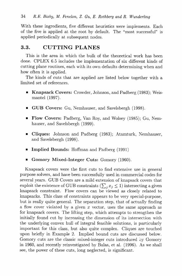
3.3. CUTTING PLANES This is the area in which the bulk of the theoretical work has been

done. CPLEX 6.5 indudes the implementation of six different kinds of cutting plane routines, each with its own defaults determining when and how often it is applied.

The kinds of cuts that are applied are listed below together with a limited set of references.

• Knapsack Covers: Crowder, Johnson, and Padberg (1983); Weismantel (1997).

• GUB Covers: Gu, Nemhauser, and Savelsbergh (1998).

• Flow Covers: Padberg, Van Roy, and Wolsey (1985); Gu, Nemhauser, and Savelsbergh (1999).

• Cliques: Johnson and Padberg (1983); Atamturk, Nemhauser, and Savelsbergh (1998).

• Implied Bounds: Hoffman and Padberg (1991)

• Gomory Mixed-Integer Cuts: Gomory (1960).

Knapsack covers were the first cuts to find extensive use in general purpose solvers, and have been successfully used in commercial codes for several years. GUB Covers are a mild extension of knapsack covers that exploit the existence of GUB constraints (Lj Xj ::; 1) intersecting a given knapsack constraint. Flow covers can be viewed as dosely related to knapsacks. This dass of constraints appears to be very special-purpose, but is really quite general. The separation step, that of actually finding a flow cover violated by a given x vector, uses the same approach as for knapsack covers. The lifting step, which attempts to strengthen the initially found cut by increasing the dimension of its intersection with the underlying convex hull of integral feasible solutions, is particularly important for this dass, but also quite complex. Cliques are touched upon briefly in Example 2. Implied bound cuts are discussed below. Gomory cuts are the dassic mixed-integer cuts introduced 'ey Gomory in 1960, and recently reinvestigated by Balas, et al. (1996). As we shall see, the power of these cuts, long neglected, is significant.


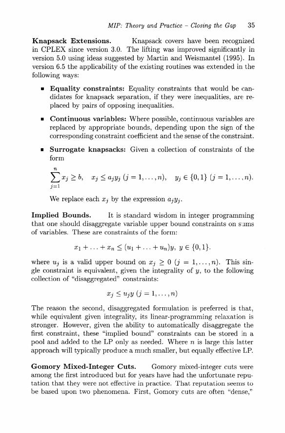
Knapsack Extensions. Knapsack covers have been recognized in CPLEX since version 3.0. The lifting was improved significantly in version 5.0 using ideas suggested by Martin and Weismantel (1995). In version 6.5 the applicability of the existing routines was extended in the following ways:

• Equality constraints: Equality constraints that would be eandidates for knapsack separation, if they were inequalities, are replaced by pairs of opposing inequalities.

• Continuous variables: Where possible, continuous variables are replaced by appropriate bounds, depending upon the sign of the corresponding constraint coefficient and the sense of the constraint.

• Surrogate knapsacks: Given a collection of constraints of the form

n

LXj b, Xj ajYj (j = 1, ... ,n), Yj E {O, I} (j = 1, ... "n). j=l

We replace each Xj by the expression ajYj.

Implied Bounds. It is standard wisdom in integer programming that one should disaggregate variable upper bound constraints on sums of variables. These are constraints of the form:

Xl + ... + Xn (UI + ... + un)y, Y E {O, I}.

where Uj is a valid upper bound on Xj ° (j = 1, ... , n). This single constraint is equivalent, given the integrality of y, to the following collection of "disaggregated" constraints:

Xj UjY (j = 1, ... ,n)

The reason the second, disaggregated formulation is preferred is that, while equivalent given integrality, its linear-programming relaxation is stronger. However, given the ability to automatically disaggregate the first constraint, these "implied bound" constraints can be stored in a pool and added to the LP only as needed. Where n is large this latter approach will typically produce a much smaller, but equally effective LP.

Gomory Mixed-Integer Cuts. Gomory mixed-integer cuts were among the first introduced but for years have had the unfortunate reputation that they were not effective in practice. That reputation seems to be based upon two phenomena. First, Gomory cuts are often "dense,"


adding a significant number of nonzeros to the constraint matrix. The linear-programming solvers of the day just couldn't handle the resulting increased density. Second, in the early tests, cuts were applied in a way that today seems obviously bad, but was quite natural at the time. Gomory's algorithm, not simply the cuts he introduced, was being viewed as a potential complete solution to integer programming, just as the simplex method was a "complete" solution for linear programming. Thus, instead of adding groups of cuts, where a group consists of as many "good" violated cuts as could be found, cuts were added one at a time, and branching was ignored. The result was that convergence was either very slow, or simply did not occur.

Times have changed. Linear-programming solvers are better and we know cuts should be added in groups; moreover, we don't expect cuts to solve the entire problem. We now realize how strong an ally intelligent branching can be. With these thoughts in mind, Gomory cuts become a very natural choice. They are the most general cuts that we have (one can always find a violated Gomory mixed-integer cut), they are easy cuts to implement, and they have the interesting, well-known property that they combine two important ideas: Rounding and disjunction. In effect, through disjunction they capture some of the effect of branching without increasing the number of active nodes.

There is a nice geometry corresponding to Gomory mixed-integer cuts, as well as a simple, straightforward algebraic derivation. Given the importance of these cuts, we sketch both.

First, the geometry. Consider a simple mixed inequality x + y 3.5, where x 0 and y is integral (not necessarily nonnegative). The feasible region for the linear-programming relaxation has exactly one fractional extreme point, (0,3.5). Removing this point is easy. We round, y l3.5 J and y f3.51, and intersect the feasible region with the resulting pair of inequalities. The result is a pair of disjoint polyhedra, in effect, a disjunction. This disjunction can be removed by taking the convex hull of the two polyhedra. Equivalently, we can add the cutting plane 2x + y 4 to the original defining inequality. This cut is exactly the associated Gomory mixed-integer cut, perhaps more properly viewed as a mixed-integer rounding cut in this case. See Wolsey for a furt her discussion of these issues.

Note that it is sometimes observed that Gomory cuts are weak relative to some of the combinatorially-derived cuts, those that can be shown to be facet defining. However, at least in this case, the Gomory cut is as strong as it can be. It defines the integer hull.


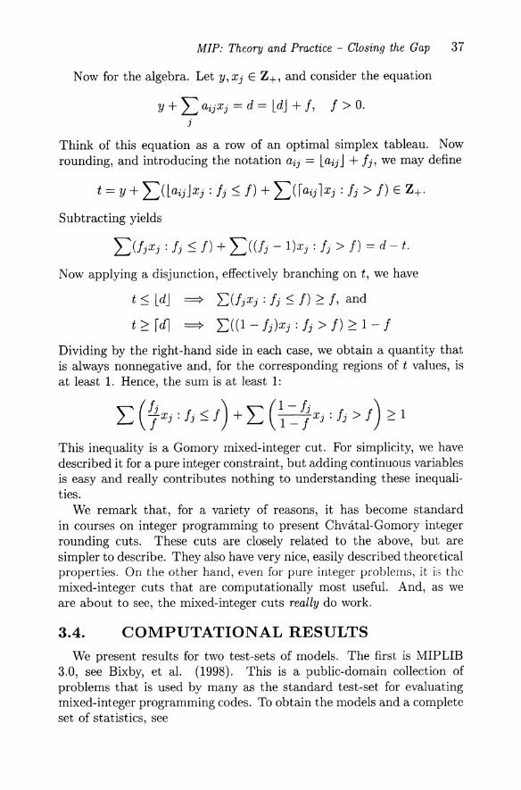
Now for the algebra. Let y, Xj E Z+, and consider the equation

y + L aijXj = d = ldJ + J, J > 0. j

Think of this equation as a row of an optimal simplex tableau. Now rounding, and introducing the notation aij = laijJ + iJ, we may define

Subtracting yields

Now applying a disjunction, effectively branching on t, we have

===? 'L(JjXj: Jj ::; J) 2: J, and

===? 2:((1 - iJ)Xj : Jj > J) 2: 1 - J

Dividing by the right-hand side in each case, we obtain a quantity that is always nonnegative and, for the corresponding regions of t values, is at least 1. Hence, the sum is at least 1:

This inequality is a Gomory mixed-integer cut. For simplicity, we have described it for a pure integer constraint, but adding continuous variables is easy and really contributes not hing to understanding these inequalities.

We remark that, for a variety of reasons, it has become standard in courses on integer programming to present Chvatal-Gomory integer rounding cuts. These cuts are closely related to the above, but are simpler to describe. They also have very nice, easily described theoretical properties. On the other hand, even far pure integer problems, it is thc mixed-integer cuts that are computationally most useful. And, as we are about to see, the mixed-integer cuts really do work.

3.4. COMPUTATIONAL RESULTS We present results for two test-sets of models. The first is MIPLIB

3.0, see Bixby, et al. (1998). This is a public-domain collection of problems that is used by many as the standard test-set for evaluating mixed-integer programming codes. To obtain the models and a complete set of statistics, see

38 R.E. Bixby, M. Fenelon, Z. Cu, E. Rothberg und R. Wunderling

http://www.caam.rice.edu/-bixby/miplib/miplib.html

We ran the following test, comparing CPLEX 6.0, which contains none of the enhancements described in this section, and CPLEX 6.5. The tests were run on a 500 MHz DEC Alpha 21264 computer with 1 Gigabyte of physical memory. Runs were made with a time limit of 7200 seconds.

The MIPLIB test-set includes 59 models. Of these 59, 22 were solved6

with both codes in less than ten seconds using default settings. Of the remaining 37, ten hit the time limit with version 6.0 but were solved with version 6.5. The geometrie me an of the CPLEX 6.5 solution times for these ten models was 48.5 seconds. Removing these ten leaves 27 models. Eight of these 27 models were solved by neither code. In these eight cases, we compared the gap between the incumbent and the best bound at termination. Version 6.0 produced a gap that was better in one case, by about 0.1 %. Taking the ratios of the percentage gaps in all eight cases, dividing the 6.0 gap by the 6.5 gap, and taking the geometrie me an yielded 3.3. Thus, the mean gap for version 6.5 was 3.3 times better. Removing the eight models that were solved by neither code left 19 models. These are the ones that were (a) reasonably hard, and (b) solvable by both codes. The geometrie mean of the solution-time ratios in this case was 11.2. That is, CPLEX 6.5 was over 11 times faster on average on these models. These results are summarized in the following table:

MIPLIB 3.0 - Defaults CPLEX 6.0 versus CPLEX 6.5

7200 second time limit

• 22 models solved by both codes in less than 10 seconds • 10 models solved by CPLEX 6.5 and not CPLEX 6.0 • 8 models solved by neither: CPLEX 6.5 3.3 times better gap • 19 models solved by both: CPLEX 6.5 11.2 times faster

There is a second test-set of largely proprietary models that we prefer to MIPLIB 3.0 in evaluating performance. This test-set was assembled about two years ago, from the CPLEX model library, in the following way. On some machine (what was then the fastest machine available to us), and using the then current version of CPLEX, we ran each model using defaults. Any model that solved to optimality in less than 100

6The default CPLEX optimality tolerance for MIPs is a gap of 0.01 %


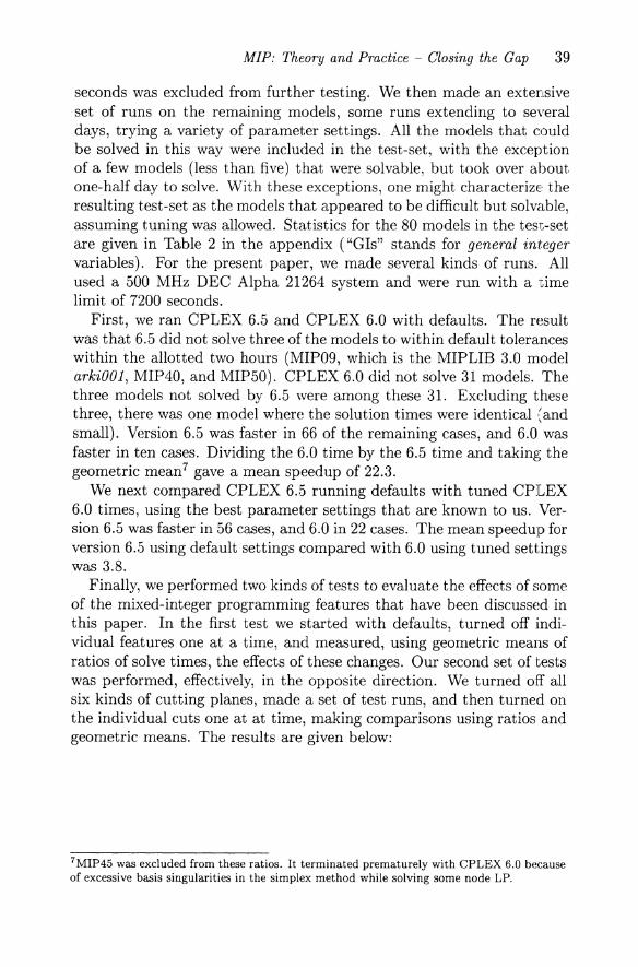
seeonds was excluded from furt her testing. We then made an extensive set of runs on the remaining models, some runs extending to seyeral days, trying a variety of parameter settings. All the models that eould be solved in this way were included in the test-set, with the exeeption of a few models (less than five) that were solvable, but took over about one-half day to solve. With these exeeptions, one might eharaeterizE' the resulting test-set as the models that appeared to be diffieult but solvable, assuming tuning was allowed. Statisties for the 80 models in the tesl;-set are given in Table 2 in the appendix ("GIs" stands for general integer variables). For the present paper, we made several kinds of runs. All used a 500 MHz DEC Alpha 21264 system and were run with aeime limit of 7200 seeonds.

First, we ran CPLEX 6.5 and CPLEX 6.0 with defaults. The result was that 6.5 did not solve three of the models to within default toleranees within the allotted two hours (MIP09, whieh is the MIPLIB 3.0 model arki001, MIP40, and MIP50). CPLEX 6.0 did not solve 31 models. The three models not solved by 6.5 were among these 31. Excluding these three, there was one model where the solution times were identieal ':and small). Version 6.5 was faster in 66 of the remaining eases, and 6.0 was faster in ten eases. Dividing the 6.0 time by the 6.5 time and taking the geometrie mean7 gave a mean speedup of 22.3.

We next eompared CPLEX 6 .. 5 running defaults with tuned CPLEX 6.0 times, using the best parameter settings that are known to uso Version 6.5 was fast er in 56 eases, and 6.0 in 22 eases. The mean speedup for version 6.5 using default settings eompared with 6.0 using tuned settings was 3.8.

Finally, we performed two kinds of tests to evaluate the effeets of so me of the mixed-integer programming features that have been diseussed in this paper. In the first test we started with defaults, turned off individual features one at a time, and measured, using geometrie means of ratios of solve times, the effeets of these ehanges. Our seeond set of tests was performed, effeetively, in the opposite direetion. We turned off all six kinds of eutting planes, made a set of test runs, and then turned on the individual euts one at at time, making eomparisons using ratios and geometrie means. The results are given below:

7MIP45 was excluded from these ratios. It terminated prematurely with CPLEX 6.0 because of excessive basis singularities in the simplex method while solving some node LP.


Performance Impact: Relative to Defaults

Cuts Implied bounds Cliques GUB covers Flow covers Covers Gomory cuts

0% 0% 0%

12% 16% 35%

Other Node presolve Node heuristics

9% 9%

Performance Impact: Individual Cuts

Implied bounds -1 % Cliques 0% GUB covers 10% Flow covers 18% Covers 58% Gomory cuts 97%

The big winner here, and perhaps the biggest surprise, was Gomory cuts. They were clearly the most effective cuts in our tests.

4. EXAMPLES We close with some examples. In the previous seetions we have at

tempted to demonstrate that great progress has been made in building general-purpose mixed-integer solvers, solvers that run well with default settings. This development is critical to the wider use of mixed-integer programming in practice. Most users of mixed-integer programming are not interested in the details of how the codes work. They simply want to be able to run a code and get results. Nevertheless, there still are, and probably always will be, many examples of interesting, important MIPs that are solvable, but not without taking advantage of problem structure in some special way.

Example 1 The first example is from a customer who was primarily interested in finding feasible solutions. His criteria was, stop after finding a feasible integral solution with gap less than 1 %. CPLEX 6.0 was incapable of meeting this criteria. Indeed, this model was left running for aperiod of several days on a fast workstation, a 600 MHz Alpha 21164 computer, and not a single feasible solution was foune. Below is a CPLEX 6.5 run for this model using a 500 MHz DEC Alpha 21264 computer:

MIP: Theory and Practice - Closing the Gap

Problem 'unnamed.mps.gz' read. Nev value for passes for generating fractional cuts: 0 Nev value for mixed integer optimality gap tolerance: 0.01 Reduced MIP has 7787 rovs, 7260 columns, and 22154 nonzeros. Clique table members: 533 Root relaxation solution time =

Nodes Node Left Objective

0 0 -2. 8298e+07 -2.776ge+07 -2. 7720e+07 -2.7703e+07 -2.768ge+07 -2.7685e+07 -2. 7685e+07

100 100 -2. 7590e+07 200 200 -2. 7446e+07

* 239 236 -2.7434e+07

GUB cover cuts applied: 6 Cover cuts applied: 44

IInf

224 160 156 176 177 180 181 58 12 0

Implied bound cuts applied: 66 Flov cuts applied: 295 Fractional cuts applied: 212

0.37 sec.

Cuts/ Best Integer Best Node

-2. 8298e+07 Cuts: 616 Cuts: 118 Cuts: 54 Cuts: 36 Cuts: 29

Flovcuts: 6 -2. 7684e+07 -2. 7684e+07

-2.7434e+07 -2. 7684e+07

ItCnt

3095 4173 4548 4790 4916 4999 5035 6174 6673 6843

Integer optimal solution (0.01/le-06): Objective = -2. 7433577522e+07 Current MIP best bound = -2.7684321743e+07 (gap = 250744, 0.91%) Solution time = 31.90 sec. Iterations = 6843 Nodes = 240 (235)

41

Gap

0.91%

So, this is an example of a model that now solves weH with default settings. One interesting aspect of the solution is that it is a case in which several features combined to produce the result. Clearly cuts were involved, and, although it is not clear from the output, the node presolve was also important. Each of several, separate features helps, but it's the combination that leads to a solution.

Example 2 Our second example illustrates how defaults are sometimes not enough. In CPLEX 6.5, several degrees of probing on binary variables are available. These options are not turned on by default. As is weH known, even with an efficient implement at ion of probing, computat ion times can experience a combinatorial explosion.

Probing occurs in three phases in CPLEX 6.5 when activated at its "highest level." In the first phase, it is applied to individual binary variables, as suggested in Brearley, et al. (1975). Thus, each binary variable is fixed in turn to 0 and then to 1, applying bound strengthening after each such fixing. For an individual variable, the result can include the fixing of the variable being probed (when one of the tested values forces the infeasibility of the whole model), implied on continuous variables-hence, implied bound cuts become stronger when


probing is activated-and 2-cliques. The 2-cliques that result from this first phase are collected and merged together with the cliques given by GUB constraints, those that are explicit in the original formulation. The result is an initial clique table. This table is then furt her expanded in a second phase by applying lifting directly to the cuts in this table. See Suhl and Szymanski (1994). This idea was suggested to us by Johnson (1999).

Finally, since, in general, there can be an exponential number of maximal cliques, it is not possible to explicitly store all such cliques. Within the branch-and-cut tree we use the clique table and the current solution to the linear-programming relaxation, as suggested by Atamturk, et al., (1998), to generate furt her clique cuts.

When we first tried to solve the present example model, it appeared not to be possible with CPLEX 6.0. The optimal objective value of the root linear-programming relaxation was 1.0, and the best-bound value never moved above 2.0, even though several parameter settings were tried and several long runs were made.

In the CPLEX 6.5 run displayed below, probing was set to its highest level. The result was that a large number of clique inequalities were generated at the root. These were crucial, pushing the lower bound at the root to 20.8. At the same time, one of the five heuristics that are applied at the root succeeded in finding a feasible solution of value 21. Since, as the output indicates, the objective function in the model could be proven to take on only integral values, it followed that 21 was optimal, and the run terminated without branching.

Problem 'unnamed.lp.gz' read. New value for probing strategy: 2 Elapsed time 10.22 sec. for 47% of probing Elapsed time 20.30 sec. for 94% of probing Probing time = 21.53 sec. Clique table members: 1068 Root relaxation solution time = 142.18 sec. Objective is integral.

Nodes Node Left Objective IInf Best Integer

0 0 1.0000 4766 20.8000 439 20.8000 203

Heuristic: feasible at 22.0000, still looking Heuristic complete * 0+ 0 21.0000 o 21. 0000

Clique cuts applied: 349

Cuts/ Best Node

1.0000 Cliques: 500 Cliques: 17

20.8000

Integer optimal solution: Objective = 2.1000000000e+01 Solution time = 792.62 sec. Iterations = 40402 Nodes = 0

ItCnt Gap 20704 36839 40402

40402 0.95%

MIP: Theory and Practice Closing the Gap 43

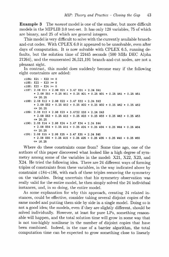
Example 3 The noswot model is one of the smaller, but more difficult models in the MIPLIB 3.0 test-set. It has only 128 variables, 75 of which are binary, and 25 of which are general integers.

This model is very difficult to solve with the currently available branchand-cut codes. With CPLEX 6.0 it appeared to be unsolvable, even after days of computation. It is now solvable with CPLEX 6.5, running defaults, but the solution time of 22445 seconds (500 Maz DEC Alpha 21264), and the enumerated 26,521,191 branch-and-cut nodes, are not a pleasant sight.

In contrast, this model does suddenly become easy if the following eight constraints are added:

e184: X2l - X22 >= 0 e185: X22 - X23 >= 0 e186: X23 - X24 >= 0 e187: 2.08 Xll + 2.98 X2l + 3.47 X3l + 2.24 X4l

+ 2.08 X5l + 0.25 Wll + 0.25 W2l + 0.25 W3l + 0.25 W4l + 0.25 W51 <= 20.25

e188: 2.08 X12 + 2.98 X22 + 3.47 X32 + 2.24 X42 + 2.08 X52 + 0.25 W12 + 0.25 W22 + 0.25 W32 + 0.25 W42 + 0.25 W52 <= 20.25

e189: 2.08 X13 + 2.98 X23 + 3.4722 X33 + 2.24 X43 + 2.08 X53 + 0.25 W13 + 0.25 W23 + 0.25 W33 + 0.25 W43 + 0.25 W53 <= 20.25

e190: 2.08 X14 + 2.98 X24 + 3.47 X34 + 2.24 X44 + 2.08 X54 + 0.25 W14 + 0.25 W24 + 0.25 W34 + 0.25 W44 + 0.25 W54 <= 20.25

e191: 2.08 X15 + 2.98 X25 + 3.47 X35 + 2.24 X45 + 2.08 X55 + 0.25 W15 + 0.25 W25 + 0.25 W35 + 0.25 W45 + 0.25 W55 <= 16.25

Where do these constraints come from? Some time ago, one of the authors of this paper discovered what looked like a high degree of symmetry among so me of the variables in the model: X21, X22, X23, and X24. He tried the following idea. There are 24 different ways of forming triples of constraints from these variables, in the way indicated above by constraint c184-c186, with each of these triples removing the symmetry on the variables. Being uncertain that his symmetry observation was really valid for the entire model, he then simply solved the 24 individual instances, and, in so doing, the entire model.

As so me explanation for why this approach, creating 24 related instances, could be effective, consider taking several disjoint copies of the same model and putting them side by side in a single model. Doing so is not a good idea; the models, even if they are slightly different, should be solved individually. However, at least for pure LPs, something reasonable will happen, and the total solution time will grow in so me way that is not too-highly non linear in the number of disjoint copies that have been combined. Indeed, in the case of a barrier algorithm, the total computation time can be expected to grow something dose to linearly


in the number of copies. However, doing this kind of replication with an integer program is an entirely different matter. There the number of nodes in the search, and hence the solution time, can be expected to grow like the product of the number of nodes in the individual search trees.

Returning to the noswot instance, the above result prompted one of OUf co-workers, Irv Lustig (1999), to "reverse engineer" the original model, and give a representation using the OPL modeling language (see Van Hentenryck (1999)). Another co-worker, Jean-Francois Puget (1999), then studied this representation and noticed that it could be given an interpretation as a reSOUfce allocation model on five machines, with scheduling, horizon constraints, and transition times. It was then clear that fOUf of the five "machines" were indeed identical, and hence that constraints c184-c186 were valid. In other words, it was necessary to solve only one of the 24 instances mentioned above. In addition, it was also observed that the transition-time constraints could be strengthened by adding five additional cuts that exploited the fact that there was actually a minimum positive transition cost of 0.25. Essentially the argument was that if a machine performs k different jobs, then it must pay at least 0.25( k - 1) in transition cost. These last constraints are also due to Puget.

With these added constraints, the model becomes solvable. Here are the results using CPLEX 6.0 and 6.5 on a 400 MHz Pentium II Laptop running a Linux operating system:

CPLEX 6.0: 142 seconds 169090 nodes CPLEX 6.5: 16 seconds 9807 nodes

So, this is a case where good modeling makes the biggest difference, but having a stronger code is also valuable.

5. SUMMARY In this paper we have discussed recent advances in linear and mixed

integer programming. The linear-programming improvements were most striking for larger models, but are effective for small and medium-sized models as weIl. One important consequence of this work is that for large models barrier algorithms are no longer dominant; each of primal and dual simplex, and barrier is now the winning choice in a significant number of cases.

For mixed-integer programming, the improvements were dramatic. These resulted from mining an extensive backlog of theoretical ideas from the scientific literatures for integer programming and combinatorial optimization. Particular attention was given to developing good default


implementations of these ideas so that they could be applied in concert, each helping on the problems to which they applied, while causing a minimal degradation in performance when they didn't apply.

Acknow ledgments The authors would like to thank John Gregory and Irv Lustig, both of ILOG,

for carefully reading this manuscript and contributing significantly to improving the exposition.

Appendix: Problem Size Statistics

Table 1 Large LP Statistics

Model Rows Columns Nonzeros Model Rows Columns Nonzeros

LP01 10295 50040 150110 LP36 30190 57000 623'730 LP02 13005 77133 361567 LP37 30258 492266 1162,)17 LP03 14188 33025 151383 LP38 31770 272372 829040 LP04 15014 37372 103866 LP39 33440 56624 16I.331 LP05 15051 34553 132295 LP40 34994 87510 208179 LP06 15349 35215 162709 LP41 35519 43582 557466 LP07 15455 59942 225514 LP42 35645 34675 208769 LP08 15540 23752 86753 LP43 36400 92878 246006 LP09 16223 28568 88340 LP44 38782 261079 1508199 LPlO 16768 39474 203112 LP45 39951 125000 381259 LP11 17681 165188 690273 LP46 41340 64162 370339 LP12 18262 23211 136324 LP47 41344 163569 1928534 LP13 18750 84375 9993717 LP48 41366 78750 2110518 LP14 19103 33490 276895 LP49 43387 107164 189864 LP15 19374 180670 5392558 LP50 43687 164831 722066 LP16 19519 45832 124280 LP51 44150 200077 4966D17 LP17 19844 55528 152952 LP52 44211 37199 321663 LP18 19999 85191 170369 LP53 47423 81915 228565 LP19 21019 115761 728432 LP54 48097 150138 1195BOO LP20 22513 99785 337746 LP55 48548 163200 617683 LP21 22797 63995 172018 LP56 54447 326504 1807146 LP22 23610 44063 154822 LP57 55020 117910 391081 LP23 23700 23005 169045 LP58 55463 191233 840986 LP24 23712 31680 81245 LP59 60384 100078 485414 LP25 24377 46592 2139096 LP60 63856 144693 717229 LP26 26618 38904 1067713 LP61 66185 157496 418321 LP27 27349 97710 288421 LP62 67745 111891 305125 LP28 27441 15128 96118 LP63 69418 612608 1722112 LP29 27899 26243 261968 LP64 72258 226090 2242086 LP30 28240 55200 161640 LP65 84840 316800 1899600 LP31 28420 164024 505253 LP66 95011 197489 749771 LP32 29002 111722 2632880 LP67 99578 326504 2102273 LP33 29017 20074 2001102 LP68 105127 154699 358171 LP34 29147 9984 1013168 LP69 108393 112955 602948 LP35 29724 98124 196524 LP70 118158 487427 974854


Table 1 (continued) Large LP Statistics

Model Rows Columns Nonzeros Model Rows Columns Nonzeros

LP71 123964 93288 459680 LP81 269640 1205640 6481640 LP72 125211 159109 457198 LP82 280756 920198 5936426 LP73 129181 467192 1025706 LP83 319256 638512 1231403 LP74 155265 377918 930166 LP84 344297 559428 1909649 LP75 175147 358239 1211488 LP85 363458 146096 11470110 LP76 179080 707556 1570514 LP86 589250 1533590 5327318 LP77 185929 189867 2787708 LP87 716772 1169910 2511088 LP78 186441 23732 397080 LP88 1000000 1685236 3370472 LP79 209760 363092 1061495 LP89 1204750 1229623 4693571 LP80 238969 772273 5795991 LP90 1709857 1903725 4959650

Table 2 Large MIP Statistics

Model Rows Columns Binaries GIs

MIP01 230 2025 1800 0 MIP02 759 17561 17561 0 MIP03 4089 121871 121870 MIP04 4116 41428 41427 1 MIP05 823 8904 8904 0 MIP06 426 7195 7195 0 MIP07 1095 11005 10940 65 MIP08 1838 807 807 0 MIP09 1048 1388 415 123 MIP10 2597 2288 1166 1122 MIP11 123 133 39 32 MIP12 105 117 34 30 MIP13 91 104 30 28 MIP14 8619 5428 1305 2 MIP15 37 526 526 0 MIP16 396 162 146 8 MIP17 631 783 28 0 MIP18 2176 6000 6000 0 MIP19 113 392 391 0 MIP20 236 1282 1277 0 MIP21 827 961 152 0 MIP22 2588 435 435 0 MIP23 15 154 0 153 MIP24 852 1337 19 0 MIP25 80 500 500 0 MIP26 4036 769 190 0 MIP27 41 49 0 30 MIP28 516 47311 47311 0 MIP29 582 55515 55515 0 MIP30 363 1298 1254 0


Table 2 (continued) Large MIP Statistics

Model Rows Columns Binaries GIs

MIP31 2291 1992 174 12 MIP32 6256 8537 197 0 MIP33 1392 1224 240 168 MIP34 1392 1224 240 168 MIP35 1248 1224 384 336

1368 1152 216 168 MIP37 1224 1152 336 336

2407 1214 802 0 MIP39 3147 2505 388 1

192 845 845 0 MIP41 1799 1008 0 1008 MIP42 43 51 0 39 MIP43 146 578 444 0 MIP44 2094 5592 443 3212 MIP45 684 1564 235 0 MIP46 68 151 150 0 MIP47 13 151 150 0 MIP48 12 151 150 0 MIP49 148 1280 1280 0 MIP50 788 645 140 0 MIP51 212 260 259 0 MIP52 2054 10724 10724 0 MIP53 908 129 31 0 MIP54 4480 10958 96 0 MIP55 291 422 98 0 MIP56 2280 1090 0 1090 MIP57 36 87482 87482 0 MIP58 176 548 548 0 MIP59 755 2756 2756 0 MIP60 45 86 55 0 MIP61 246 240 64 0 MIP62 1192 840 48 0 MIP63 2984 1451 1451 0 MIP64 291 556 300 15 MIP65 249 690 690 0 MIP66 314 5111 41 0 MIP67 20022 17665 17664 0 MIP68 23259 29342 13215 0 MIP69 524 1197 1100 96 MIP70 331 45 45 0 MIP71 146 578 444 0 MIP72 42 17419 17419 0 MIP73 3228 15541 15540 0 MIP74 1359 1959 0 1959 MIP75 234 378 168 0 MIP76 234 378 168 0 MIP77 4277 2417 1364 0 MIP78 845 3345 235 0 MIP79 10108 3836 1862 0 MIP80 27 26306 26306 0


References

[1] E. D. Anderson and K. D. Anderson (1995), Presolving in Linear Programming, Mathematical Programming, 71, No. 2, pp. 221-245.

[2J A. At amt urk, G. L. Nemhauser and M. W. P. Savelsbergh (1998), Conflict Graphs in Integer Programming, Report LEC-98-03, Georgia Institute of Technology.

[3] E. Balas, S. Ceria, G. Cornueljols and N. Natraj (1996), Gomory Cuts Revisited, Operations Research Letters, 19, pp. 1-10.

[4J R. E. Bixby, S. Ceria, C. M. McZeal and M. W. P. Savelsbergh (1998), An Updated Mixed Integer Programming Library: MIPLIB 3.0, Optima, 54, pp. 12-15.

[5] A. L. Brearley, G. Mitra and H. P. Williams (1975), Analysis of Mathematical Programming Problems Prior to Applying the Simplex Algorithm, Mathematical Programming, 8, pp. 54-83.

[6] W. J. Carolan, J. E. Hill, J. L. Kennington, S. Niemi and S. J. Wichmann (1990), An Empirical Evaluation of the KORBX Algorithms for Military Airlift Applications, Operations Research, 38, No. 2, pp. 240-248.

[7J V. ChvataJ (1983). Linear Programming, Freeman, New York. [8J H. P. Crowder, E. L. Johnson and M. W. Padberg (1983), Solving

Large-Scale Zero-One Linear Programming Problems, Operations Research, 31, pp. 803-834.

[9] J. R. Gilbert and T. Peierls (1988), Sparse Partial Pivoting in Time Proportional to Arithmetic Operations, SJSSC, 9, pp. 862-874.

[10J R. E. Gomory (1960), An Algorithm for the Mixed Integer Problem, RM-2597, The Rand Corporation.

[l1J Z. Gu, G. L. Nemhauser and M. W. P. Savelsbergh (1998), Lifted Cover Inequalities for 0-1 Integer Programs, INFORMS Journal on Computing, 10, pp. 417-426.

[12] Z. Gu, G. L. Nemhauser and M. W. P. Savelsbergh (1999), Lifted Flow Covers for Mixed 0-1 Integer Programs, Mathematical Programming, 85, pp. 439-467.

[13J K. Hoffman and M. Padberg (1991), Improving Representations of Zero-one Linear Programs for Branch-and-Cut, ORSA Journal 0/ Computing, 3, pp. 121-134.

[14J E. Johnson (1999), Private communication. [15J E. 1. Johnson and M. W. Padberg (1983), Degree-two Inequalities,

Clique Facets, and Bipartite Graphs, Annals 0/ Discrete Mathematics, 16, pp. 169-188.


[16] A. H. Land and A. G. Doig (1960), An Automatie Method for Solving Diserete Programming Problems, Econometrica, 28, pp. 497-520.

[17] 1. J. Lustig (1999), Private communication.

[18] R. E. Marsten (1981), XMP: A Structured Library of Subroutines for Experimental Mathematical Programming, ACM Transactions on Mathematical Software, 7, pp. 481-497.

[19] A. Martin and R. Weismantel (1995), Private communication.

[20] M. W. Padberg, T. J. Van Roy and L. A. Wolsey (1985), Valid Linear Inequalities for Fixed Charged Problems, Operations ReseaTch, 33, pp. 842-86l.

[21] Jean-Francois Puget (1999), Private communication.

[22] E. Rothberg and A. Gupta (1991), Efficient Sparse Matrix Factorization on High Performance Workstations-Exploiting the Memory Hierarchy, ACM Transactions on Mathematical SoftwaTe, 17, No. 3, pp. 313-334.

[23] E. Rothberg and B. Hendrickson (1998), Sparse Matrix Ordering Methods for Interior Point Linear Programming, INFORMS Journalon Computing, 10, No. 1, pp. 107-113.

[24] M. W. P. Savelsbergh (1994), Preproeessing and Probing for Mixed Integer Programming Problems, ORSA Journal on Computing, 6, pp. 445-454.

[25] U. H. Suhl and R. Szymanski (1994), Supernode Processing of Mixed-Integer Models, Computational Optimization and Applications, 3, pp. 317-33l.

[26] P. Van Hentenryck (1999), The OPL Optimization Programming Language, MIT Press.

[27] R. Weismantel (1997), On the 0/1 Knapsack Polytope, Mathematical Programming, 77, pp. 49--68.

[28] L. A. Wolsey (1998), Integer Programming, Wiley.

Documents

MIP: THEORY AND PRACTICE CLOSING THE GAP - Springer