Embed Size (px)
Citation preview
Map Projections Used by the U.S. Geological Survey
GEOLOGICAL SURVEY BULLETIN 1532
Map Projections Used by the U.S. Geological Survey By JOHN P. SNYDER
GEOLOGICAL SURVEY BULLETIN 1532
Second Edz'tz"on
UNITED STATES GOVERNMENT PRINTING OFFICE, WASHil''GTON:1982
DEPARTMENT OF THE INTERIOR
WILLIAM P. CLARK, Secretary
U.S. GEOLOGICAL SURVEY
Dallas L. Peck, Director
First edition, 1982 Second edition, 1983
Second edition reprinted, 1984
Library of C9ngress Cataloging in Publication Data
Snyder, John Parr, 1926-Map projections used by the U.S. Geological Survey.
(Geological Survey bulletin ; 1532) Bibliography: p. Supt. of Docs. no.: I 19.3:1532 1. Map-projection. 2. United States. Geological Survey. I. Title. II. Series. QE75.B9 no. 1532 [GAllO] 557.3s [526.8] 81-607569 AACR2
For sale by the Superintendent of Documents, U.S. Government Printing OfCjce Washington, D.C. 20402
PREFACE TO SECOND EDITION
This study of map projections is intended to be useful to both the reader interested in the philosophy or history of the projections and the reader desiring the mathematics. Under each of the sixteen r¥ojections described, the nonmathematical phases are presented first, YTithout interruption by formulas. They are followed by the formulas r.nd tables, which the first type of reader may skip entirely to pass to the nonmathematical discussion of the next projection. Even with the mathematics, there are almost no derivations, very little calculus, and no complex variables or matrices. The emphasis is on desc:--ibing the characteristics of the projection and how it is used.
This bulletin is also designed so that the user can turn dire~tly to the desired projection, without reading any other section, in order to study the projection under consideration. However, the list of synbols may be needed in any case, and the random-access feature will be enhanced by a general understanding of the concepts of projections and distortion. As a result of this intent, there is some repetition which will be apparent as the book is read sequentially.
Many of the formulas and much of the history and general discussion are adapted from a source manuscript I prepared shortly before joining the U.S. Geological Survey. The relationship of the projecthns to the Survey has been incorporated as a result of the generous cooperation of several Survey personnel. These include Alden P. Colvocoresses, William J. Jones, Clark H. Cramer, Marlys K. Brownlee, Tau Rho Alpha, Raymond M. Batson, William H. Chapman, Atef .A • Elassal, Douglas M. Kinney (ret.), George Y. G. Lee, Jack P. Minta (ret.), and John F. W aananen. Joel L. Morrison of the University of Wisconsin/Madison and Allen J. Pope of the National Ocean Survey also made many helpful comments.
Many of the inverse formulas, and a few others, have been derived in conjunction with this study. Many of the formulas may be found in other sources; however, many, especially inverse formulaf:, are frequently omitted or are included in more cumbersome form elsewhere. All formulas adapted from other sources have been tested for accuracy.
For the more complicated projections, equations are given in the order of usage. Otherwise, major equations are given first, followed by subordinate equations. When an equation has been given previously, it is repeated with the original equation number, to avoid the need to leaf back and forth. A compromise in this philosophy is the placing of numerical examples in appendix A. It was felt that placing these with the formulas would only add to the difficulty of reading through the mathematical sections.
III
IV
The need for a working manual of this type has led to an uneroectedly early exhausting of the supply of the first edition of this bulletin. In this new edition there are minor revisions and corrections noted to date. These primarily consist of corrections to equations (15-10) on p. 129 and (20-22) on p. 204 and replacement of the inverse van der Grinten algorithm on p. 215-216 with that developed by Rubincam. The former algorithm is also accurate, but very cumbersome. In addition, historical notes have been corrected on p. 23, 144, ana 219.
Further corrections and comments by users are most welcome. It is hoped that this study provides a practical reference for those C'lncerned with map projections.
Reston, Va. May 1983
John P. Snyder
CONTENTS
Preface to Second Edition-----------------------------------------------
Symbols -----------------------------------------------------------Acronyms -----------------------------------------------------·----Abstract------------------------------------------------------------Introduction ________________________________________________________ _
Map projections-general concepts --------------------------------------1. Characteristics of map projections---------------------------------2. Longitude and latitude -------------------------------------~----3. The datum and the Earth as an ellipsoid-----------------------~----
Auxiliary latitudes ------------------------------------------4. Scale variation and angular distortion ------------------------------
Tissot's indicatrix --------------------------------------·----Distortion for projection of the sphere ----------------------~---Distortion for projection of the ellipsoid -------------------------
5. Transformation of map graticules ----------------------------~----6. Classification of map projections-----------------------------------
Cylindrical map projections -·-------------------------------------------7. Mercator projection ---------------------------------------------
Summary -------------------------------------------------History----------------------------------------------------Features and usage -----------------------------------------Formulas for the sphere -------------------------------------Formulas for the ellipsoid------------------------------------Mercator projection with another standard parallel ----------------
8. Transverse Mercator projection -----------------------------------Summary -----------------------------·--------------------History----------------------------------------------------Features -------------------------------------------------Usage-----------------------------------------------------Universal Transverse Mercator projection ----------------------Formulas for the sphere -------------------------------------Formulas for the ellipsoid------------------------------------"Modified Transverse Mercator'' projection -----------------------
Formulas for the "Modified Transverse Mercator'' projection -----9. Oblique Mercator projection--------------------------------------
Summary -------------------------------------------------History----------------------------------------------------Features -------------------------------------------------Usage-----------------------------------------------------Formulas for the sphere -------------------------------------Formulas for the ellipsoid -------------------------------------
10. Miller Cylindrical projection--------------------------------------
Summary --------------------------------------------------History and features -----------------------------------------Formulas for the sphere ------------------------------------·--
Page
III XI
XIII 1 1 5 5
11 13 16 23 23 25 28 33 39 41 43 43 43 45 47 50 51 53 53 53 55 55 63 64 67 69 72 73 73 73 74 76 76 78 85 85 85 87
v
VI CONTENTS
Page
Cylindrical map projections- Continued 11. Equidistant Cylindrical projection--------------------------------- 89
Summary -------------------------------------------------- 89 History and features ----------------------------------------- 89 Formulas for the sphere -------------------·------------------- 90
Conic map projections---------------~---------------------------------- 91 12. Albers Equal-Area Conic projection------------------------------- 93
Summary -------------------------------------------------- 93 History ---------------------------------------------------- 93 Features and usage ------------------------------------------ 93 Formulas for the sphere -------------------------------------- 95 Formulas for the ellipsoid ------------------------------------- 96
13. Lambert Conformal Conic projection------------------------------ 101 Summary --------------------------------------------------- 101 History---------------------------------------------------- 101 Features -------------------------------------------------- 101 Usage ----------------------------------------------------- 103 Formulas for the sphere-------------------------------------- 105 Formulas for the ellipsoid------------------------------------- 107
14. Bipolar Oblique Conic Conformal projection------------------------- 111 Summary -------------------------------------------------- 111 History---------------------------------------------------- 111 Features and usage ----------------------------------------- 113 Formulas for the sphere -------------------------------------- 114
15. Polyconic projection -------------------------------------------- 123 Summary -------------------------------------------------- 123 History---------------------------------------------------- 123 Features -------------------------------------------------- 124 Usage ----------------------------------------------------- 126 Geometric construction--------------------------------------- 128 Formulas for the sphere --------------------------------- ----- 128 Formulas for the ellipsoid ------------------------------------- 129 Modified Polyconic for the International Map of the World ---------- 133
Azimuthal map projections --------------------------------------------- 135 16. Orthographic projection----------------------------------------- 141
Summary -------------------------------------------------- 141 History ---------------------------------------------------- 141 Features ----------------------------------------------·--- 141 Usage ------------·----------------------------------------- 144 Geometric construction--------------------------------------- 144 Formulas for the sphere-------------------------------------- 146
17. Stereographic projection ---------------------------------------- 153 Summary -------------------------------------------------- 153 History---------------------------------------------------- 153 Features -------------------------------------------------- 154 Usage ----------------------------------------------------- 156 Formulas for the sphere -------------------------------------- 158 Formulas for the ellipsoid ------------------------------------- 160
18. Lambert Azimuthal Equal-Area projection-------------------------- 167 Summary -------------------------------------------------- 167 History---------------------------------------------------- 167
CONTENTS VII
Page
Azimuthal map projections-Continued 18. Lambert Azimuthal Equal-Area projection-Continued
Features -------------------------------------------------- 167 Usage ---------------------------------------------------- 170 Geometric construction-------------------------------------- 170 Formulas for the sphere -------------------------------------- 170 Formulas for the ellipsoid------------------------------------ 173
19. Azimuthal Equidistant projection --------------------------------- 179 Summary ----------------------------------------------- 179 History----------------------------------------------·---- 179 Features ---------------------------------------------- 180 Usage -------------------------------------------------- 182 Geometric construction-------------------------------------- 182 Formulas for the sphere -------------------------------------- 184 Formulas for the ellipsoid----------------------------------- 185
Space map projections------------------------------------------------- 193 20. Space Oblique Mercator projection------------------------------- 193
Surnnmary -------------------------------------------------- 193 History------------------------------- --------------------- 193 Features and usage ------------------------------------------ 194 Formulas for the sphere ----------------------------------·---- 198 Formulas for the ellipsoid ------------------------------------- 203
Miscellaneous map projections------------------------------------------ 211 21. Van der Grinten projection --------------------------------------- 211
Summary -------------------------------------------------- 211 History, features, and usage----------------------------------- 211 Geometric construction--------------------------------------- 213 Formulas for the sphere-------------------------------------- 214
22. Sinusoidal projection---------------------------------------·---- 219 Summary -------------------------------------------------- 219 History---------------------------------------------------- 219 Features and usage ------------------------------------------ 221 Formulas for the sphere -------------------------------------- 222
AppendiKes --------------------------------------------------------- 223 A. Numerical examples -------------------------------------------- 225 B. Use of map projections by U.S. Geological Survey-Summary---------- 301
References---------------------------------------------------------- 303 Index -------------------------------------------------------------- 307
ILLUSTRATIONS
Page
FIGURE 1. Projections of the Earth onto the three major surfaces ----------- 8 2. Meridians and parallels on the sphere-------------------------- 14 3. Tissot's indicatrix ------------------------------------------ 24 4. Distortion patterns on common conformal map projections -------- 26 5. Spherical triangle ------------------------------------------ 36 6. Rotation of a graticule for transformation of projection ----------- 37 7. Gerhard us Mercator---------------------------------------- 44
VIII CONTENTS
Page
FIGURE 8. The Mercator projection ------------------------------------ 46 9. Johann Heinrich Lambert----------------------------------- 54
10. The Transverse Mercator projection-------------------------- 57 11. Universal Transverse Mercator grid zone designations for the world 65 12. Oblique Mercator projection --------------------------------- 75 13. Coordinate system for the Hotine Oblique Mercator projection ------ 82 14. The Miller Cylindrical projection----------------------------- 86 15. Albers Equal-Area Conic projection--------------------------- 94 16. Lambert Conformal Conic projection--------------------------- 102 17. Bipolar Oblique Conic Conformal projection -------------------- 119 18. Ferdinand Rudolph Hassler--------------------------------- 124 19. North America on a Polyconic projection grid------------------- 125 20. Geometric projection of the parallels of the polar Orthographic rro-
jection ------------------------------------------------- 142 21. Orthographic projection: (A) polar aspect, (B) equatorial aspect,
(C) oblique aspect---------------------------------------- 143 22. Geometric construction of polar, equatorial, and oblique Ortho-
graphic projections--------------------------------------- 145 23. Geometric projection of the polar Stereographic projection -------- 154 24. Stereographic projection: (A) polar aspect, (B) equatorial aspect,
(C) oblique aspect---------------------------------------- 155 25. Lambert Azimuthal Equal-Area projection: (A) polar aspect, (B) eq•,a-
torial aspect, (C) oblique aspect----------------------------- 169 26. Geometric construction of polar Lambert Azimuthal Equal-Area
projection ---------------------------------------------- 171 27. Azimuthal Equidistant projection: (A) polar aspect, (B) equato~ial
aspect, (C) oblique aspect---------------------------------- 183 28. Two orbits of the Space Oblique Mercator projection ------------- 196 29. One quadrant of the Space Oblique Mercator projection----------- 197 30. Vander Grinten projection---------------------------------- 212 31. Geometric construction of the Van der Grinten projection --------- 213 32. Interrupted Sinusoidal projection ----------------------------- 220
1-1402. Map showing the properties and uses of selected map projections, by Tau Rho Alpha and John P. Snyder ___________________________ In pocket
TABLES
Page
TABLE 1. Some official ellipsoids in use throughout the world--------------- 15 2. Official :figures for extraterrestrial mapping -------------------- 17 3. Corrections for auxiliary latitudes on the Clarke 1866 ellipsoid ----- 22 4. Lengths of 1° of latitude and longitude on two ellipsoids of reference 29 5. Ellipsoidal correction factors to apply to spherical projections baqed
on Clarke 1866 ellipsoid----------------------------------- 31 6. Mercator projection: Used for extraterrestrial mapping----------- 48 7. Mercator projection: Rectangular coordinates ------------------- 52 8. U.S. State plane coordinate systems--------------------------- 58 9. Universal Transverse Mercator grid coordinates----------------- 66
CONTENTS IX
Page
TABLE 10. Transverse Mercator projection: Rectangular coordinates for the
sphere -------------------------------------------------- 70 11. Universal Transverse Mercator projection: Location of point:~ with
given scale factor ----------------------------------------- 71 12. Hotine Oblique Mercator projection parameters used for Lancsat 1,
2, and 3 imagery ------------------------------------------ 77 13. Miller Cylindrical projection: Rectangular coordinates ------------- 88 14. Albers Equal-Area Conic projection: Polar coordinates------------ 99 15. Lambert Conformal Conic projection: Used for extraterr':!strial
mapping ------------------------------------------------ 106 16. Lambert Conformal Conic projection: Polar coordinates----------- 112 17. Bipolar Oblique Conic Conformal projection: Rectangular coordinates 120 18. Polyconic projection: Rectangular coordinates for the Clarke. 1866
ellipsoid ------------------------------------------------ 131 19. Comparison of major azimuthal projections---------------------- 137 20. Orthographic projection: Rectangular coordinates for equrtorial
aspect ·------------------------------------------------- 148 21. Orthographic projection: Rectangular coordinates for oblique aspect
centered at lat. 40° N ------------------------------------- 149 22. Polar Stereographic projection: Used for extraterrestrial mappir~ __ 157 23. Stereographic projection: Rectangular coordinates for equatorial
aspect -------------------------------------------------- 161 24. Ellipsoidal polar Stereographic projection----------------------- 165 25. Lambert Azimuthal Equal-Area projection: Rectangular coord~"'ates
forequatorialaspect--------------------------------------- 174 26. Ellipsoidal polar Lambert Azimuthal Equal-Area projection-------- 177 27. Azimuthal Equidistant projection: Rectangular coordinates for equa-
torial aspect --------------------------------------------- 186 28. Ellipsoidal Azimuthal Equidistant projection-polar aspect--------- 187 29. Plane coordinate systems for Micronesia ------------------------ 190 30. Scale factors for the spherical Space Oblique Mercator proj':!ction
using Landsat constants------------------------------------ 202 31. Scale factors for the ellipsoidal Space Oblique Mercator proj':!ction
using Landsat constants------------------------------------ 210 32. Van d~r Grin ten projection: Rectangular coordinates -------------- 216

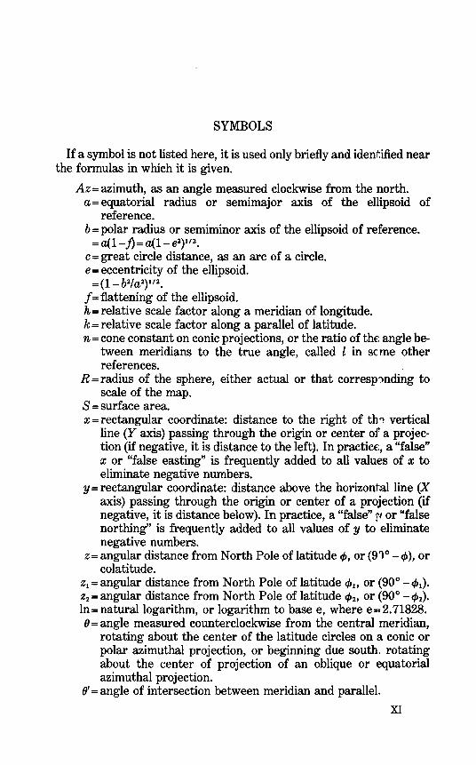
SYMBOLS
If a symbol is not listed here, it is used only briefly and identified near the formulas in which it is given.
Az =azimuth, as an angle measured clockwise from the north. a= equatorial radius or semimajor axis of the ellipsoid of
reference. b =polar radius or semiminor axis of the ellipsoid of reference. = a(1-fJ = a(1- el)t'l.
c = great circle distance, as an arc of a circle. e = eccentricity of the ellipsoid. = (1- bl/ a2)112.
f= flattening of the ellipsoid. h = relative scale factor along a meridian of longitude. k = relative scale factor along a parallel of latitude. n = cone constant on conic projections, or the ratio of the: angle be
tween meridians to the true angle, called l in scme other references.
R =radius of the sphere, either actual or that corresp1nding to scale of the map.
S =surface area. x =rectangular coordinate: distance to the right of th~ vertical
line (Y axis) passing through the origin or center of a projection (if negative, it is distance to the left). In practice:, a "false" x or "false easting" is frequently added to all values of x to eliminate negative numbers.
y = rectangular coordinate: distance above the horizontal line (X axis) passing through the origin or center of a projection (if negative, it is distance below). In practice, a "false" ?' or "false northing" is frequently added to all values of y to eliminate negative numbers.
Z= angular distance from North Pole of latitude cp, or (91° -cp), or colatitude.
z1 =angular distance from North Pole of latitude cp., or (90°- cp1).
z2 =angular distance from North Pole of latitude c/>2 , or (90°- c/>2).
In= natural logarithm, or logarithm to base e, where e = 2. 71828. 8 =angle measured counterclockwise from the central meridian,
rotating about the center of the latitude circles on a conic or polar azimuthal projection, or beginning due south, rotating about the center of projection of an oblique or equatorial azimuthal projection.
8' = angle of intersection between meridian and paralleL
XI
XII MAP PROJECTIONS USED BY THE USGS
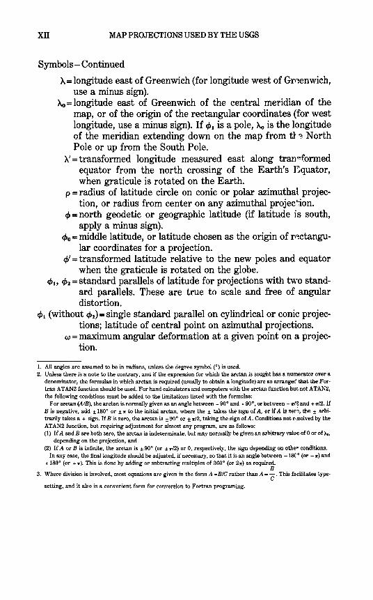
Symbols-Continued
A= longitude east of Greenwich (for longitude west of Grr~enwich, use a minus sign).
Ac, =longitude east of Greenwich of the central meridian of the map, or of the origin of the rectangular coordinates (for west longitude, use a minus sign). If c/> 1 is a pole, Ac, is the longitude of the meridian extending down on the map from tl'~ North Pole or up from the South Pole.
A'= transformed longitude measured east along tran~formed equator from the north crossing of the Earth's I:quator, when graticule is rotated on the Earth.
p = radius of latitude circle on conic or polar azimuthal projection, or radius from center on any azimuthal projec~ion.
cp = north geodetic or geographic latitude (if latitude j s south, apply a minus sign).
c/>0 = middle latitude, or latitude chosen as the origin of r~~ctangular coordinates for a projection.
cp' = transformed latitude relative to the new poles and equator when the graticule is rotated on the globe.
cp., c/>z = standard parallels of latitude for projections with two standard parallels. These are true to scale and free of angular distortion.
cJ>. (without c/>2) =single standard parallel on cylindrical or conic projections; latitude of central point on azimuthal projections.
w =maximum angular deformation at a given point on a projection.
1. All angles are assumed to be in radians, unless the degree symbol (0) is used.
2. Unless there is a note to the contrary, and if the expression for which the arctan is sought has a numerator over a denominator, the formulas in which arctan is required (usually to obtain a longitude) are so arranged that the For· tran ATAN2 function should be used. For hand calculators and computers with the arctan function but not ATAN2, the following conditions must be added to the limitations listed with the formulas:
For arctan (A/B), the arctan is normally given as an angle between -90° and + 90°, or between - w/2 and + w/2. If B is negative, add ± 180° or ± w to the initial arctan, where the ± takes the sign of A, or if A is zer1, the ± arbitrarily takes a + sign. If B is zero, the arctan is ± 90° or ± w/2, taking the sign of A. Conditions not r<>.solved by the ATAN2 function, but requiring adjustment for almost any program, are as follows: (1) If A and B are both zero, the arctan is indeterminate, but may normally be given an arbitrary value of 0 or of~.
depending on the projection, and (2) If A orB is infinite, the arctan is ± 90° (or ± w/2) or 0, respectively, the sign depending on othe,. conditions.
In any case, the final longitude should be adjusted, if necessary, so that it is an angle between - 18('0 (or - w) and + 180° (or + w). This is done by adding or subtracting multiples of 360° (or 2.,.-) as required.
B 3. Where division is involved, most equations are given in the form A =BIG rather than A= C. This facilitates type-
setting, and it also is a convenient form for conversion to Fortran programing.
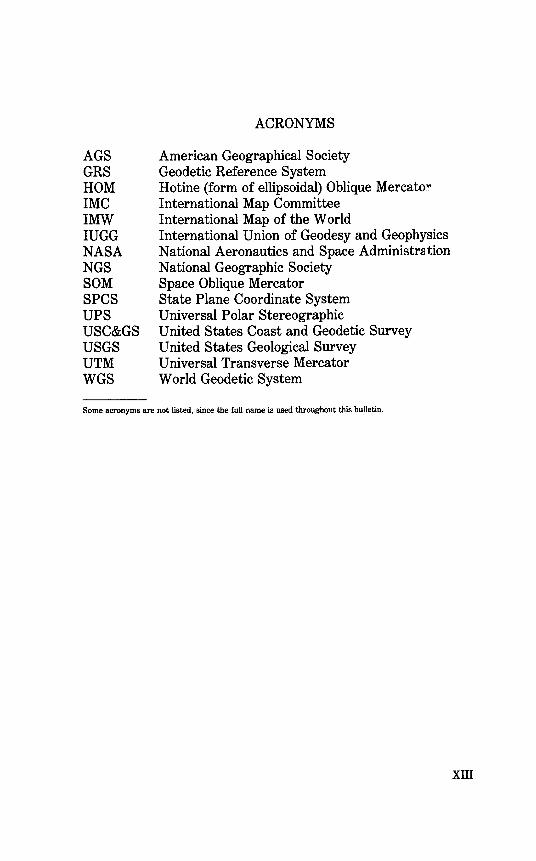
AGS GRS HOM IMC IMW IUGG NASA NGS SOM SPCS UPS USC&GS USGS UTM WGS
ACRONYMS
American Geographical Society Geodetic Reference System Hotine (form of ellipsoidal) Oblique Mercato~ International Map Committee International Map of the World International Union of Geodesy and Geophysics National Aeronautics and Space Administration National Geographic Society Space Oblique Mercator State Plane Coordinate System Universal Polar Stereographic United States Coast and Geodetic Survey United States Geological Survey Universal Transverse Mercator World Geodetic System
Some acronyms are not listed, since the full name is used throughout this bulletin.
XIII

MAP PROJECTIONS USED BY THE
U.S. GEOLOGICAL SURVEY
By JOHN P. SNYDER
ABSTRACT
After decades of using only one map projection, the Polyconic, for its I"lapping program, the U.S. Geological Survey (USGS) now uses sixteen of the more comnon map projections for its published maps. For larger scale maps, including topographic quadrangles and the State Base Map Series, conformal projections such as the Transve~se Mercator and the Lambert Conformal Conic are used. On these, the shapes of sm1.ll areas are shown correctly, but scale is correct only along one or two lines. Equal-are~. projections, especially the Albers Equal-Area Conic, and equidistant projections which have correct scale along many lines appear in the National Atlas. Other projections, such as the Miller Cylindrical and the Van der Grin ten, are chosen occasionally for convenienc,~. sometimes making use of existing base maps prepared by others. Some projections treat the Earth only as a sphere, others as either ellipsoid or sphere.
The USGS has also conceived and designed several new projections, hcluding the Space Oblique Mercator, the first map projection designed to permit ma"')ping of the Earth continuously from a satellite with low distortion. The mapping of extraterrestrial bodies has resulted in the use of standard projections in completely new settings.
With increased computerization, it is important to realize that rectangular coordinates for all these projections may be mathematically calculated with formulas which would have seemed too complicated in the past, but which now may be programed routinely, if clearly delineated with numerical examples. A discussion of appearance, usage, and history is given together with both forward and inverse equations for each projection involved.
INTRODUCTION
The subject of map projections, either generally or specif~ally, has been discussed in thousands of papers and books dating at least from the time of the Greek astronomer Claudius Ptolemy (about A.D.150 ), and projections are known to have been in use some three centuries earlier. Most of the widely used projections date from the 16th to 19th centuries, but scores of variations have been developed durin:~ the 20th century. Within the past 10 years, there have been several ne"v publications of widely varying depth and quality devoted exclusiv~ly to the
1
2 MAP PROJECTIONS USED BY THE USGS
subject (Alpha and Gerin, 1978; Hilliard and others, 1978; Le~, 1976; Maling, 1973; McDonnell, 1979; Pearson, 1977; Rahman, 1974; Richardus and Adler, 1972; Wray, 1974). In 1979, the USGS p•1blished Maps for America, a book-length description of its maps (Thompson, 1979).
In spite of all this literature, there has been no definitive single publication on map projections used by the USGS, the agency r~sponsible for administering the National Mapping Program. The UrGS has relied on map projection treatises published by the former Coast and Geodetic Survey (now the National Ocean Survey). These publications do not include sufficient detail for all the major projections usei by the USGS. A widely used and outstanding treatise of the Coast and Geodetic Survey (Deetz and Adams, 1934), last revised in 19~5, only touches upon the Transverse Mercator, now a commonly used projection for preparing maps. Other projections such as the Bipolar Oblique Conic Conformal, the Miller Cylindrical, and the Van der Grinten, were just being developed, or, if older, were seldom used in 1945. Deetz and Adams predated the extensive use of the computer and pocket calculator, and, instead, offered extensive tables for plotting projections with specific parameters.
Another classic treatise from the Coast and Geodetic Sur,.rey was written by Thomas (1952) and is exclusively devoted to the five major conformal projections. It emphasizes derivations with a summary of formulas and of the history of these projections, and is directed toward the skilled technical user. Omitted are tables, graticules, or numerical examples.
In this bulletin, the author undertakes to describe each pr')jection which has been used by the USGS sufficiently to permit the skilled mathematically oriented cartographer to use the projection in detail. The descriptions are also arranged so as to enable a lay pe ... son interested in the subject to learn as much as desired about the pr'nciples of these projections without being overwhelmed by mathematical detail. Deetz and Adams' work sets an excellent example in this combined approach.
Since this study is limited to map projections used by the USGS, several map projections frequently seen in atlases and geograplty texts have been omitted. The general formulas and concepts are usef'll, however, in studying these other projections. Many tables of rectansmar or polar coordinates have been included for conceptual purpm,es. For values between points, formulas should be used, rather than interpolation. Other tables list definitive parameters for use in formulas.
The USGS, soon after its official inception in 1879, apparently chose the Polyconic projection for its mapping program. This projection is simple to construct and had been promoted by the Survey of th~ Coast, as it was then called, since Ferdinand Rudolph Hassler's leadership of
INTRODUCTION 3
the early 1800's. The first published USGS topographic "quadrangles," or maps bounded by two meridians and two parallels, did not carry a projection name, but identification as "Polyconic projection'r w~s added to later editions. Tables of coordinates published by the USGS appeared by 1904, and the Polyconic was the only projection mentioned by Beaman (1928, p. 167).
Mappers in the Coast and Geodetic Survey, influenced in turn by military and civilian mappers of Europe, established the ~'tate Plane Coordinate System in the 1930's. This system involved tte Lambert Conformal Conic projection for States of larger east-west extension and the Transverse Mercator for States which were longer from north to south. In the late 1950's, the USGS began changing q·1adrangles from the Polyconic to the projection used in the State Plane Coordinate System for the principal State on the map. The USGS also friopted the Lambert for its series of State base maps.
As the variety of maps issued by the USGS increased, a broad range of projections became important: The Polar Stereographic for the map of Antarctica, the Lambert Azimuthal Equal-Area for maps of the Pacific Ocean, and the Albers Equal-Area Conic for National Atlas (USGS, 1970) maps of the United States. Several other projections have been used for other maps in theNationalAtlas, for tec~onic maps, and for grids in the panhandle of Alaska. The mapping of extraterrestrial bodies, such as the Moon, Mars, and Mercury, involves old projections in a completely new setting. The most recent projection promoted by the USGS and perhaps the first to be originatec1 within the USGS is the Space Oblique Mercator for continuous mapping using artificial satellite imagery (Snyder, 1981).
It is hoped that this study will assist readers to understanc better not only the basis for maps issued by the USGS, but also the pri"'lciples and formulas for computerization, preparation of new maps, and transferring of data between maps prepared on different projections.

MAP PROJECTIONS-GENERAL CONCEPT~
1. CHARACTERISTICS OF MAP PROJECTIONS
The general purpose of map projections and the basic problems encountered have been discussed often and well in various books on cartography and map projections. (Robinson, Sale, and Mor~ison, 1978; Steers, 1970; and Greenhood, 1964, are among recent editions of earlier standard references.) It is necessary to mention tl'~ concepts, but to do so concisely, although there are some interpretathns and formulas that appear to be unique.
For almost 500 years, it has been conclusively established that the Earth is essentially a sphere, although there were a numbe"" of intellectuals nearly 2,000 years earlier who were convinced of this. Even to the scholars who considered the Earth flat, the skies appeared hemispherical, however. It was established at an early date that attempts to prepare a flat map of a surface curving in all directions leads to distortion of one form or another.
A map projection is a device for producing all or part of a round body on a flat sheet. Since this cannot be done without distorthn, the cartographer must choose the characteristic which is to be: shown accurately at the expense of others, or a compromise of several characteristics. There is literally an infinite number of ways ir which this can be done, and several hundred projections have beer published, most of which are rarely used novelties .. Most projections may be infinitely varied by choosing different points on the Earth a~ the center or as a starting point.
It cannot be said that there is one "best" projection for mapping. It is even risky to claim that one has found the "best" projection for a given application, unless the parameters chosen are artificially c-:mstricting. Even a carefully constructed globe is not the best map for rr.ost applications because its scale is by necessity too small. A straight(ldge cannot be satisfactorily used for measurement of distance, and it is awkward to use in general.
The characteristics normally considered in choosing a map projection are as follows:
1. A rea. Many map projections are designed to be equal-a'~'"ea, so that a coin, for example, on one part of the map covers exactly the same area of the actual Earth as the same coin on any other part of the map. Shapes, angles, and scale must be distorted on most parts of such a map, but there are usually some parts of an equal-area map which are designed to retain these characteristics correctly, or very nearly so.
5
6 MAP PROJECTIONS USED BY THE USGS
Less common terms used for equal-area projections are equivalent, homolographic, or homalographic (from the Greek homalos or homos ("same") and graphos ("write")); authalic (from the Greek autos ("s-:~.me") and ailos ("area'')), and equiareal.
2. Shape. Many of the most common and most important projections are conformal or orthomorphic (from the Greek orthos or "straight" and morphe or "shape"), in that normally the shape of every small feat'1re of the map is shown correctly. (On a conformal map of the entire Earth there are usually one or more "singular" points at which shape is still distorted.) A large landmass must still be shown distorted in fhape, even though its small features are shaped correctly. An important result of conformality is that relative angles at each point are correct, and the local scale in every direction around any one point is con~tant. Consequently, meridians intersect parallels at right (90°) angles on a conformal projection, just as they do on the Earth. Areas are gen~rally enlarged or reduced throughout the map, but they are relativel:T correct along certain lines, depending on the projection. Nearly all largescale maps of the Geological Survey and other mapping agencies throughout the world are now prepared on a conformal projection.
3. Scale. No map projection shows scale correctly throughout the map, but there are usually one or more lines on the map along which the scale remains true. By choosing the locations of these lines properly, the scale errors elsewhere may be minimized, although some errors may still be large, depending on the size of the area being mapped and the projection. Some projections show true scale between one or two points and every other point on the map, or along every meridian. They are called "equidistant" projections.
4. Direction. While conformal maps give the relative local dire~~tions correctly at any given point, there is one frequently used group of map projections, called azimuthal (or zenithal), on which the directions or azimuths of all points on the map are shown correctly with resp~ct to the center. One of these projections is also equal-area, another i;;- conformal, and another is equidistant. There are also projections on which directions from two points are correct, or on which directions from all points to one or two selected points are correct, but these are rarely used.
5. Special characteristics. Several map projections provide suecial characteristics that no other projection provides. On the Mercator projection, all rhumb lines, or lines of constant direction, are shown as straight lines. On the Gnomonic projection, all great circle paths- the shortest routes between points on a sphere- are shown as straight lines. On the Stereographic, all small circles, as well as great circles, are shown as circles on the map. Some newer projections are specially designed for satellite mapping. Less useful but mathematically intrigu-
MAP PROJECTIONS- GENERAL CONCEPTS 7
ing projections have been designed to fit the sphere conformally into a square, an ellipse, a triangle, or some other geometric figure.
6. Method of construction. In the days before ready acc~ss to computers and plotters, ease of construction was of greater importance. With the advent of computers and even pocket calculator~.' very complicated formulas can be handled almost as routinely as simple projections in the past.
While the above features should ordinarily be considered in choosing a map projection, they are not so obvious in recognizing a p~ojection. In fact, if the region shown on a map is not much larger thar the United States, for example, even a trained eye cannot often distinguish whether the map is equal-area or conformal. It is necessary to make measurements to detect small differences in spacing or location of meridians and parallels, or to make other tests. The type of construction of the map projection is more easily recognized with e;'"perience, if the projection falls into one of the common categories.
There are three- types of developable1 surfaces onto whicl' most of the map projections used by the USGS are at least partially gf~ometrically projected. They are the cylinder, the cone, and the plane. Actually all three are variations of the cone. A cylinder is a limiting form of a cone with an increasingly sharp point or apex. As the cone becc~es flatter, its limit is a plane.
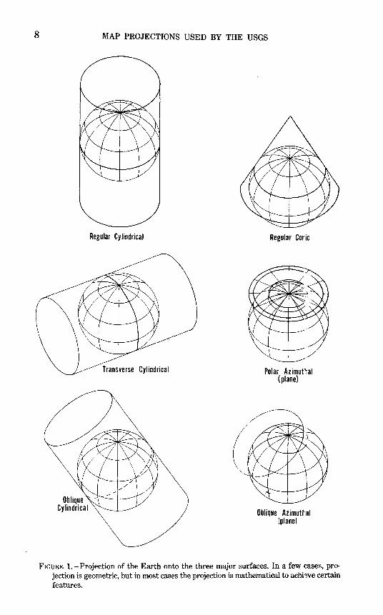
If a cylinder is wrapped around the globe representing the Earth, so that its surface touches the Equator throughout its circumference, the meridians of longitude may be projected onto the cylinder as equidistant straight lines perpendicular to the Equator, and the parallels of latitude marked as lines parallel to the Equator, around the circumference of the cylinder and mathematically spaced for certain characteristics. When the cylinder is cut along some meridian and unrolled, a cylindrical projection with straight meridians and straight parallels results (see fig. 1). The Mercator projection is the best-known example.
If a cone is placed over the globe, with its peak or apE:x along the polar axis of the Earth and with the surface of the cone touching the globe along some particular parallel of latitude, a conic (or conical) projection can be produced. This time the meridians are projected onto the cone as equidistant straight lines radiating from the ap~x, and the parallels are marked as lines around the circumference of the cone in planes perpendicular to the Earth's axis, spaced for the desired characteristics. When the cone is cut along a meridian, unrolled, and laid flat, the meridians remain straight radiating lines, but the parallels are now circular arcs centered on the apex. The angles between meridians are shown smaller than the true angles.
1 A developable surface is one that can be transformed to a plane without distortion.
8 MAP PROJECTIONS USED BY THE USGS
Regular Cylindrical Regular Coric
Polar Azimunal (plane)
Oblique Azimuttal (plane)
FIGURE 1.-Projection of the Earth onto the three major surfaces. In a few cases, projection is geometric, but in most cases the projection is mathematical to achi~ve certain features.
MAP PROJECTIONS-GENERAL CONCEPTS 9
A plane tangent to one of the Earth's poles is the ba~is for polar azimuthal projections. In this case, the group of projections is named for the function, not the plane, since all common tangent-l)lane projections of the sphere are azimuthal. The meridians are projected as straight lines radiating from a point, but they are spaced at their true angles instead of the smaller angles of the conic proj qctions. The parallels of latitude are complete circles, centered on the p')le. On some important azimuthal projections, such as the Stereographic (for the sphere), the parallels are geometrically projected from a common point of perspective; on others, such as the Azimuthal Equidistant, they are nonperspective.
The concepts outlined above may be modified in two ways, which still provide cylindrical, conic, or azimuthal projections (although the azimuthals retain this property precisely only for the sphere). (1) The cylinder or cone may be secant to or cut the flobe at two parallels instead of being tangent to just one. This conceptually provides two standard parallels; but for most conic projections this construction is not geometrically correct. The plane may likewise cut through the globe at any parallel instead of touching a pc 1e. (2) The axis of the cylinder or cone can have a direction di~erent from that of the Earth's axis, while the plane may be tangent to a point other than a pole (fig. 1). This type of modification leads to impor~ant oblique, transverse, and equatorial projections, in which most meridians and parallels are no longer straight lines or arcs of circles. What were standard parallels in the normal orientation now become standard lines not following parallels of latitude.
Some other projections used by the USGS resemble one C""" another of these categories only in some respects. The Sinusoidal projection is called pseudocylindrical because its latitude lines are parallel and straight, but its meridians are curved. The Polyconic proje~tion is projected onto cones tangent to each parallel of latitude, so tre meridians are curved, not straight. Still others are more remotely rel2ted to cylindrical, conic, or azimuthal projections, if at all.

2. LONGITUDE AND LATITUDE
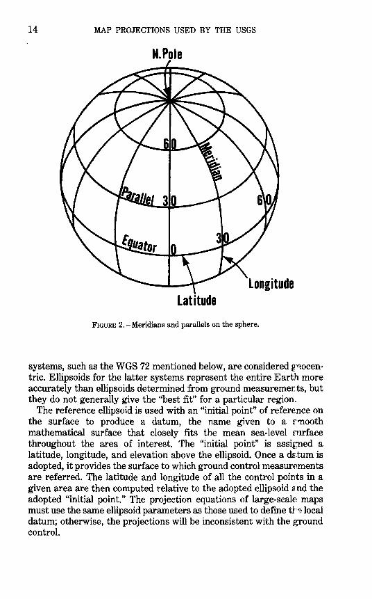
To identify the location of points on the Earth, a graticule or network of longitude and latitude lines has been superimposed on the surface. They are commonly referred to as meridians and parallels, respectively. Given the North and South Poles, which are approximately the ends of the axis about which the Earth rotates, and the Equator, an imaginary line halfway between the two poles, the parallels of latitude are formed by circles surrounding the Earth and in planes pr-J.rallel with that of the Equator. If circles are drawn equally spaced ak11g the surface of the sphere, with 90 spaces from the Equator to each pole, each space is called a degree of latitude. The circles are numbered from 0° at the Equator to 90° North and South at the respective poles. Each degree is subdivided into 60 minutes and each minute into 60 seconds of arc.
Meridians of longitude are formed with a series of imaginary lines, all intersecting at both the North and South Poles, and crossing each parallel of latitude at right angles, but striking the Equato~ at various points. If the Equator is equally divided into 360 parts, and a meridian passes through each mark, 360 degrees of longitude re<:'•1lt. These degrees are also divided into minutes and seconds. While the length of a degree of latitude is always the same on a sphere, the. lengths of degrees of longitude vary with the latitude (see fig. 2). At the Equator on the sphere, they are the same length as the degree of t~.titude, but elsewhere they are shorter.
There is only one location for the Equator and poles which serve as references for counting degrees of latitude, but there is no natural origin from which to count degrees of longitude, since all m~ridians are identical in shape and size. It, thus, becomes necessary to choose arbitrarily one meridian as the starting point, or prime meriiian. There have been many prime meridians in the course of history, swayed by national pride and international influence. Eighteenth-cent·u'Y maps of the American colonies often show longitude from London or Philadelphia. During the 19th century, boundaries of new States were described with longitudes west of a meridian through Washington, D.C., 77°03'02.3" west of the Greenwich (England) Prim~ Meridian, which was increasingly referenced on 19th century_maps (VanZandt, 1976, p. 3). In 1884, the International Meridian Conference, meeting in Washington, agreed to adopt the "meridian passing througl:t the center of the transit instrument at the Observatory of Greenwich as the initial meridian for longitude," resolving that "from this meridian longitude
11
12 MAP PROJECTIONS USED BY THE USGS
shall be counted in two directions up to 180 degrees, east longitude being plus and west longitude minus" (Brown, 1949, p. 297).
When constructing meridians on a map projection, the central meridian, usually a straight line, is frequently taken to be the starting point or 0° longitude for calculation purposes. When the map is completed with labels, the meridians are marked with respect to the Greenwich Prime Meridian. The formulas in this bulletin are arranged so that Greenwich longitude may be used directly.
The concept of latitudes and longitudes was originated early in recorded history by Greek and Egyptian scientists, especiall:· the Greek astronomer Hipparchus (2nd century, B.C.). Claudius Ptolemy further formalized the concept (Brown, 1949, p. 50, 52, 68).
Because calculations relating latitude and longitude to positions of points on a given map can become quite involved, rectangular grids have been developed for the use of surveyors. In this way, each point may be designated merely by its distance from two perpendicular axes on the flat map.
3. THE DATUM AND THE EARTH AS AN ELLIPSOID
For many maps, including nearly all maps in commercial atlases, it may be assumed that the Earth is a sphere. Actually, it is more nearly an oblate ellipsoid of revolution, also called an oblate spher1id. This is an ellipse rotated about its shorter axis. The flattening of the ellipse for the Ea.~. ~his only about one part in three hundred; but it is s·1fficient to become a r:ecessary part of calculations in plotting accurate maps at a scale of 1:100,000 or larger, and IS significant even for 1:5,000,000-scale maps of the United States, affecting plotted shapes by up to 2/a percent. On small-scale maps, including single-sheet world maps, the oblateness is negligible. Formulas for both the sphere and ellipsoid will be discussed in this bulletin wherever the pr0jection is used in both forms.
The Earth is not an exact ellipsoid, and deviations from this shape are continually evaluated. For map projections, however, tl'~ problem has been confined to selecting constants for the ellipsoidal shape and size and has not generally been extended to incorporating the much smaller deviations from this shape, except that different reference ellipsoids are used for the mapping of different regions of the Earth.
An official shape of the ellipsoid was defined in 1924, wher the International Union of Geodesy and Geophysics (IUGG) adopted a flattening of exactly 1 part in 297 and a semimajor axis (or equatorial radius) of exactly 6,378,388 m. The radius of the Earth along the pclar axis is then 1/297less than 6,378,388, or approximately 6,356,911.~ m. This is called the International ellipsoid and is based on J ohr Fillmore Hayford's calculations in 1909 from U.S. Coast and Geodei-ic Survey measurements made entirely within the United States (Brown, 1949, p. 293; Hayford, 1909). This ellipsoid was not adopted for use in North America.
There are over a dozen other principal ellipsoids, however, which are still used by one or more countries (table 1). The different c1;mensions do not only result from varying accuracy in the geodetic measurements (the measurements of locations on the Earth), but the curvature of the Earth's surface is not uniform due to irregularities in the gravity field.
Until recently, ellipsoids were only fitted to the Earth's sh~.oe over a particular country or continent. The polar axis of the reference ellipsoid for such a region, therefore, normally does not coincid ~ with the axis of the actual Earth, although it is made parallel. The same applies to the two equatorial planes. The discrepancy between cente:':"s is usually a few hundred meters at most. Only satellite-determined coordinate
13
14 MAP PROJECTIONS USED BY THE USGS
N.Pole
Longitude Latitude
FIGURE 2. -Meridians and parallels on the sphere.
systems, such as the WGS 72 mentioned below, are considered g~ocentric. Ellipsoids for the latter systems represent the entire Earth more accurately than ellipsoids determined from ground measuremeiJ ts, but they do not generally give the "best fit" for a particular region.
The reference ellipsoid is used with an "initial point" of reference on the surface to produce a datum, the name given to a f'llooth mathematical surface that closely fits the mean sea-level rarface throughout the area of interest. The "initial point" is assigned a latitude, longitude, and elevation above the ellipsoid. Once a dz.tum is adopted, it provides the surface to which ground control measurements are referred. The latitude and longitude of all the control points in a given area are then computed relative to the adopted ellipsoid znd the adopted "initial point." The projection equations of large-scale maps must use the same ellipsoid parameters as those used to define tl'o.local datum; otherwise, the projections will be inconsistent with the ground control.
MAP PROJECTIONS-GENERAL CONCEPTS 15
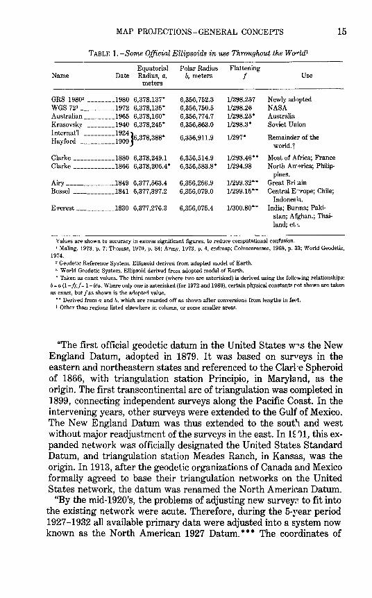
TABLE 1.-Some Official Ellipsoids in use Throughout the Wo'f'ld1
Equatorial Polar Radius Flattening Name Date Radius, a, b, meters f Use
meters
GRS 19802 ________ 1980 6,378,137* 6,356, 752.3 11298.257 Newly adopted WGS 723 __________ 1972 6,378,135* 6,356, 750.5 11298.26 NASA Australian _________ 1965 6,378,160* 6,356, 77 4. 7 11298.25* Australia Krasovsky ________ 1940 6,378,245* 6,356,863.0 1/298.3* Soviet Union Internat'l _________ 1924 }
6,378
,388
• 6,356,911.9 11297* Remainder of the Hayford __________ 1909
world.t
Clarke ____________ 1880 6,378,249.1 6,356,514.9 11293.46** Most of Africa; France Clarke ____________ 1866 6,378,206.4 * 6,356,583.8* 1/294.98 North Arr"!rica; Philip-
pines. Airy ______________ 1849 6,377,563.4 6,356,256.9 11299.32** Great Bri'ain Bessel ____________ 1841 6,377,397.2 6,356,079.0 11299.15** Central E 'rope; Chile;
Indonesia. Everest ___________ 1830 6,377,276.3 6,356,075.4 11300.80** India; Burma; Paki-
stan; Afghan.; Thai-land; et~.
Values are shown to accuracy in excess significant figures, to reduce computational confusion. 1 Maling, 1973, p. 7; Thomas, 1970, p. 84; Army, 1973, p. 4, endmap; Colvocoresses, 1969, p. 33; World Geodetic,
1974. 2 Geodetic Reference System. Ellipsoid derived from adopted model of Earth. 3 World Geodetic System. Ellipsoid derived from adopted model of Earth. • Taken as exact values. The third number (where two are asterisked) is derived using the follC'wing relationships:
b=a (1-.f);f= 1- bla. Where only one is asterisked (for 1972 and 1980), certain physical constants rot shown are taken as exact, but f as shown is the adopted value.
• • Derived from a and b, which are rounded off as shown after conversions from lengths in feet. t Other than regions listed elsewhere in column, or some smaller areas.
"The first official geodetic datum in the United States w<;l.s the New England Datum, adopted in 1879. It was based on surveys in the eastern and northeastern states and referenced to the Clarl·e Spheroid of 1866, with triangulation station Principio, in Maryland, as the origin. The first transcontinental arc of triangulation was completed in 1899, connecting independent surveys along the Pacific Coast. In the intervening years, other surveys were extended to the Gulf of Mexico. The New England Datum was thus extended to the sout':t and west without major readjustment of the surveys in the east. In lf11, this expanded network was officially designated the United States Standard Datum, and triangulation station Meades Ranch, in Kansas, was the origin. In 1913, after the geodetic organizations of Canada and Mexico formally agreed to base their triangulation networks on the United States network, the datum was renamed the North Amerir.an Datum.
"By the mid-1920's, the problems of adjusting new survey~ to fit into the existing network were acute. Therefore, during the 5-year period 1927-1932 all available primary data were adjusted into a system now known as the North American 1927 Datum.*** The coordinates of
16 MAP PROJECTIONS USED BY THE USGS
station Meades Ranch were not changed but the revised coordirates of the network comprised the North American 1927 Datum" (National Academy of Sciences, 1971, p. 7 ).
The ellipsoid adopted for use in North America is the result of the 1866 evaluation by the British geodesist Alexander Ross Clarke using measurements made by others of meridian arcs in western E'lrope, Russia, India, South Africa, and Peru (Clarke and Helmert, 1911, p. 807 -808). This resulted in an adopted equatorial radius of 6,378,206.4 m and a polar radius of 6,356,583.8 m, or an approximate flatte--:1ing of 1/294.9787. Since Clarke is also known for an 1880 revision used in Africa, the Clarke 1866 ellipsoid is identified with the year.
Satellite tracking data have provided geodesists witt new measurements to define the best Earth-fitting ellipsoid and for r~lating existing coordinate systems to the Earth's center of mass. The I ~fense Mapping Agency's efforts produced the World Geodetic System 1966 (WGS 66), followed by a more recent evaluation (1972) produc~ng the WGS 72. The polar axis of the Clarke 1866 ellipsoid, as used with the North American 1927 Datum, is calculated to be 159 m from that of WGS 72. The equatorial planes are 176 m apart (World G~odetic System Committee, 1974, p. 30).
Work is underway at the National Geodetic Survey to replace the North American 1927 Datum. The new datum, expected to be called "North American Datum 1983," will be Earth-centered based on satellite tracking data. The IUGG early in 1980 adopted a new model of the Earth called the Geodetic Reference System (GRS) 1980, from which is derived an ellipsoid very similar to that for the WGS 72; it is expected that this ellipsoid will be adopted for the new North An1erican datum.
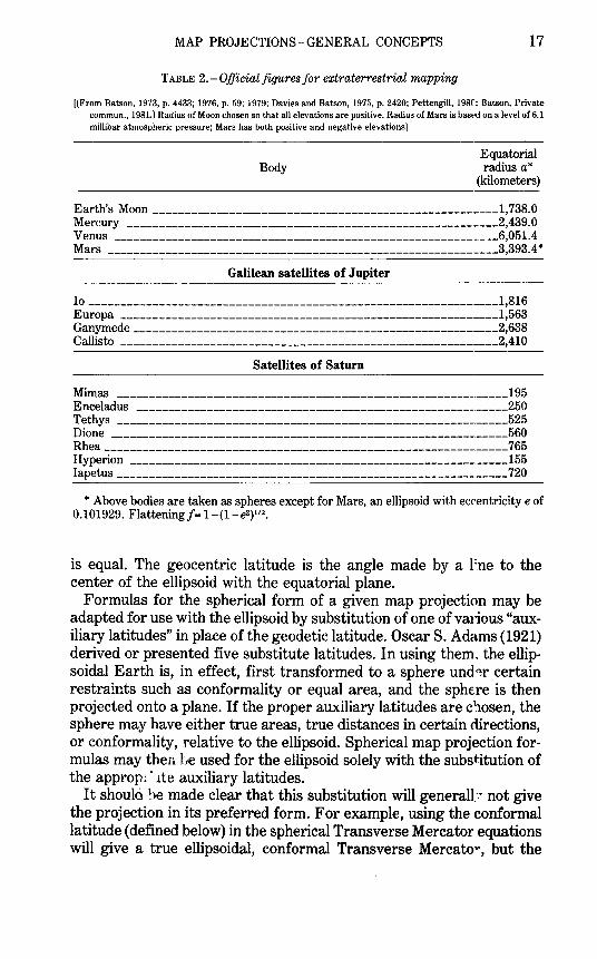
For the mapping of other planets and natural satellites, only T 1ars is treated as an ellipsoid. The Moon, Mercury, Venus, and the satellites of Jupiter and Saturn are taken as spheres (table 2).
In most map projection formulas, some form of the eccentricity e is used, rather than the flattening f. The relationship is as follows:
e2 = 2/-f 2 , or f= 1-(1- e2)112
For the Clarke 1866, e2 is 0.006768658.
AUXILIARY LATITUDES
By definition, the geographic or geodetic latitude, which is nC'~mally the latitude referred to for a point on the Earth, is the angle which a line perpendicular to the surface of the ellipsoid at the given point makes with the plane of the Equator. It is slightly greater in magnitude than the geocentric latitude, except at the Equator and poles, where it
MAP PROJECTIONS-GENERAL CONCEPTS 17
TABLE 2.-Official figures for extraterrestrial mapping
[(From Batson, 1973, p. 4433; 1976, p. 59; 1979; Davies and Batson, 1975, p. 2420; Pettengill, 198{'; Batson, Private commun., 1981.) Radius of Moon chosen so that all elevations are positive. Radius of Mars is based on a level of 6.1 millibar atmospheric pressure; Mars has both positive and negative elevations]
Body Equatorial radius a*
(kilometers)
Earth's Moon ------------------------------------------------------1,738.0 Mercury ------------------------------------------------------·----2,439.0 Venus ------------------------------------------------------------6,051.4 Mars -------------------------------------------------------------3,393.4*
Galilean satellites of Jupiter
Io ------------------------------------------------------------·----1 ,816 Europa -----------------------------------------------------------1,563 Ganymede _________________________________________________________ 2,638
Callisto -----------------------------------------------------------2,410
Satellites of Saturn
Mirnas -------------------------------------------------------------195 Enceladus ----------------------------------------------------------250 Tethys -------------------------------------------------------------525 Dione --------------------------------------------------------------560 Rhea _______________________________________________________________ 765
Hyperion ------------------------------------------------------------155 Iapetus _____________________________________________________________ 720
* Above bodies are taken as spheres except for Mars, an ellipsoid with eccentricity e of 0.101929. Flattening f= 1-(1- &)112
•
is equal. The geocentric latitude is the angle made by a l:ne to the center of the ellipsoid with the equatorial plane.
Formulas for the spherical form of a given map projection may be adapted for use with the ellipsoid by substitution of one of various "auxiliary latitudes" in place of the geodetic latitude. Oscar S. Adams (1921) derived or presented five substitute latitudes. In using them~ the ellipsoidal Earth is, in effect, first transformed to a sphere und~r certain restraints such as conformality or equal area, and the sphere is then projected onto a plane. If the proper auxiliary latitudes are ct10sen, the sphere may have either true areas, true distances in certain directions, or conformality, relative to the ellipsoid. Spherical map projection formulas may then be used for the ellipsoid solely with the subst.itution of the approp:. · J.te auxiliary latitudes.
It shoulri 1Je made clear that this substitution will generalb~ not give the projection in its preferred form. For example, using the conformal latitude (defined below) in the spherical Transverse Mercator equations will give a true ellipsoidal, conformal Transverse Mercato•, but the
18 MAP PROJECTIONS USED BY THE USGS
central meridian cannot be true to scale. More involved formulas are necessary, since uniform scale on the central meridian is a stardard requirement for this projection as commonly used in the ellipsoic,~l form. For the regular Mercator, on the other hand, simple substitution of the conformal latitude is sufficient to obtain both conformality and an Equator of correct scale for the ellipsoid.
Adams gave formulas for all these auxiliary latitudes in closed or exact form, as well as in series, except for the authalic (equal-area) latitude, which could also have been given in closed form. Both forms are given below. In finding the auxiliary latitude from the geodetic latitude, the closed form may be more useful for computer pr'"lgrams. For the inverse cases, to find geodetic from auxiliary latitudes, most closed forms require iteration, so that the series form is probr l:lly preferable. The series form shows more readily the amount of d~viation from the geodetic latitude cp. The formulas given later for the individual ellipsoidal projections incorporate these formulas as needed, so there is no need to refer back to these for computation, but the various auxiliary latitudes are grouped together here for comparison.
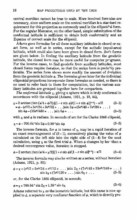
The conformal latitude x, giving a sphere which is truly conformal in accordance with the ellipsoid (Adams, 1921, p. 18, 84),
x = 2 arctan (tan (1r/4 + cp/2)[(1- e sin cp)/(1 + e sin cp)]e12} -1r/2 (3-1) = cp- ( e2/2 + 5e4/24 + 3e6/32 + ... )sin 2cp + (5e4/ 48 + 7 eG/80 + ... )
sin 4cp- (13e6/480 + ... )sin 6cp + . . . (3-2)
with x and cp in radians. In seconds of arc for the Clarke 1866 €.Hipsoid,
x=c/J -700.04"sin 2cp+ 0.99"sin 4cp (3-3)
The inverse formula, for cp in terms of x, may be a rapid iteration of an exact rearrangement of (3-1), successively placing the value of cp calculated on the left side into the right side of (3- 4) for the next calculation, using x as the first trial cp. When cp changes by les" than a desired convergence value, iteration is stopped.
cp= 2 arctan {tan (11"14+ x/2)[(1 + e sin cp)/(1- e sin cp)]e12} -11"/2 (3-4)
The inverse formula may also be written as a series, without iteration (Adams, 1921, p. 85):
c/J=x+(e2/2+5e4/24+e6/12+ ... )sin 2x+(7e4/48+29e6/240+ ... ) sin 4x + (7 eG/120 + ... ) sin 6x + . . . (3-5)
or, for the Clarke 1866 ellipsoid, in seconds,
c/J=x+700.04" sin 2x+ 1.39" sin 4x (3-6)
Adams referred to x as the isometric latitude, but this name is now applied tot/;, a separate very nonlinear function of cp, which is directly pro-
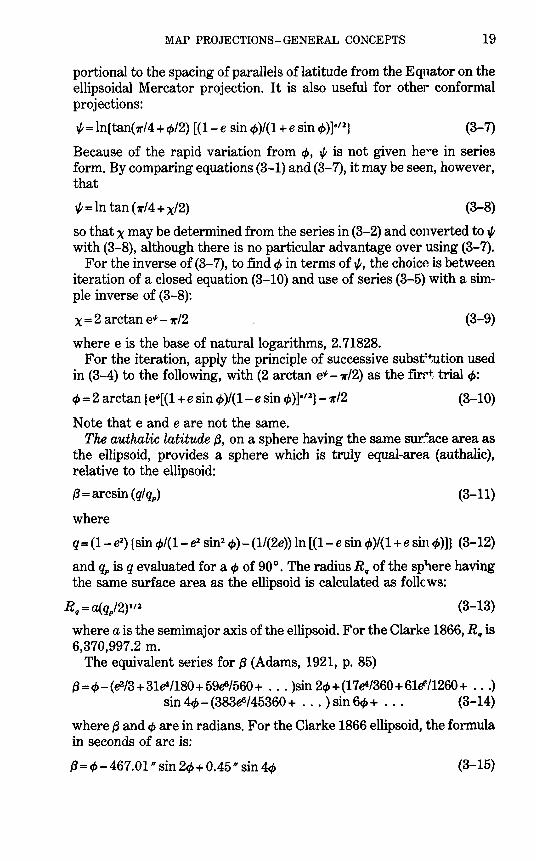
MAP PROJECTIONS- GENERAL CONCEPTS 19
portional to the spacing of parallels of latitude from the Equator on the ellipsoidal Mercator projection. It is also useful for other conformal projections:
,Y =In[ tan( 1rl4 + ¢/2) [(1- e sin cp )/(1 + e sin cp )]•' 2} (3-7)
Because of the rapid variation from ¢, ,Y is not given he•e in series form. By comparing equations (3-1) and (3-7), it may be seen, however, that
,Y =In tan ( 1rl 4 + x/2) (3-8)
so that x may be determined from the series in (3-2) and converted to ,Y with (3-8), although there is no particular advantage over using (3-7).
For the inverse of (3-7), to find cp in terms of 1/;, the choice is between iteration of a closed equation (3-10) and use of series (3-5) with a simple inverse of (3-8):
x = 2 arctan e"'- 1rl2 (3-9)
where e is the base of natural logarithms, 2. 71828. For the iteration, apply the principle of successive subsf~tion used
in (3-4) to the following, with (2 arctan e"'- 1r/2) as the firri:. trial ¢:
cf>= 2 arctan [e"'[(1 + e sin ¢)/(1- e sin ¢)]•'2} -?r/2 (3-10)
Note that e and e are not the same. The authalic latitude 13, on a sphere having the same surface area as
the ellipsoid, provides a sphere which is truly equal-area (authalic), relative to the ellipsoid:
13 = arcsin ( q/ qp) (3-11)
where
q= (1- e2) [sin ¢/(1- e2 sin2 ¢)- (1/(2e)) In [(1- e sin ¢)/(1 + e sin¢)]} (3-12)
and qp is q evaluated for a cp of 90°. The radius R9 of the sp'lere having the same surface area as the ellipsoid is calculated as foll()ws:
(3-13)
where a is the semimajor axis of the ellipsoid. For the Clarke 1866, R9 is 6,370,997.2 m.
The equivalent series for 13 (Adams, 1921, p. 85)
13=¢-(e2/3+31e4/180+59e6/560+ ... )sin 2¢+(17e4/360+61lf/1260+ ... ) sin4¢-(383e6/45360+ ... )sin6¢+... (3-14)
where 13 and cp are in radians. For the Clarke 1866 ellipsoid, the formula in seconds of arc is:
{3=¢-467.01" sin 2¢+0.45" sin 4¢ (3-15)
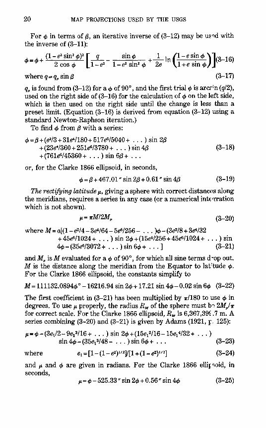
20 MAP PROJECTIONS USED BY THE USGS
For <Pin terms of (3, an iterative inverse of (3-12) may be us~d with the inverse of (3-11):
<P=<P+ (1- e2 sin
2 cp)
2 [-q- _ sin~ +-1-ln (1- e si.n <P )]<3_16) 2 cos q, 1- e2 1-e2 sm2 q, 2e 1 + e s1n <P
where q = qp sin {3 (3-17)
qp is found from (3-12) for a q, of 90°, and the first trial <Pis arcr'n (q/2), used on the right side of (3-16) for the calculation of <P on the left side, which is then used on the right side until the change is less than a preset limit. (Equation (3-16) is derived from equation (3-12) using a standard Newton-Raphson iteration.)
To find cp from {3 with a series:
cp = {3 + ( e2/3 + 31e4/180 + 517 eG/5040 + ... ) sin 2{3 + (23e"/360 + 251&/3780 + ... ) sin 4{3 + (761&/45360 + ... ) sin 6{3 + ...
or, for the Clarke 1866 ellipsoid, in seconds,
<P = {3 + 467.01 II sin 2{3 + 0.61 11 sin 4{3
(3-18)
(3-19)
The rectifying latitude p., giving a sphere with correct distances along the meridians, requires a series in any case (or a numerical inkqration which is not shown).
p. = 1rMI2Mp (3-20)
where M = a[(1- e2/4- 3e4/64- 5&/256- ... )<P- (3e2/8 + 3e4/32 + 45&/1024 + ... ) sin 2<P + (15e4/256 + 45&/1024 + ... ) sin 4q,- (35&/3072 + ... ) sin 6cp + ... ] (3-21)
and Mp isM evaluated for a cp of 90°, for which all sine terms d':"op out. M is the distance along the meridian from the Equator to laftude cp. For the Clarke 1866 ellipsoid, the constants simplify to
M = 111132.0894cp0 -16216.94 sin 2<P+ 17.21 sin 4cp-0.02 sin 6cp (3-22)
The first coefficient in (3-21) has been multiplied by 7r/180 to use <Pin degrees. To use p. properly, the radius RM of the sphere must b~ 2Mpl1r for correct scale. For the Clarke 1866 ellipsoid, RM is 6,367,39£. 7 m. A series combining (3-20) and (3-21) is given by Adams (1921, :r" 125):
p.=cp-(3e1/2-9e13/16+ ... ) sin 2cp+(15e1
2/16-15e14/32+ ... )
sin 4cp- (35e13/ 48- ... ) sin 6cp + ...
where
(3-23)
(3-24)
and p. and <P are given in radians. For the Clarke 1866 elli:r~oid, in seconds,
p.=cp-525.33 11 sin 2cp+0.56 11 sin 4cp (3-25)
MAP PROJECTIONS-GENERAL CONCEPTS 21
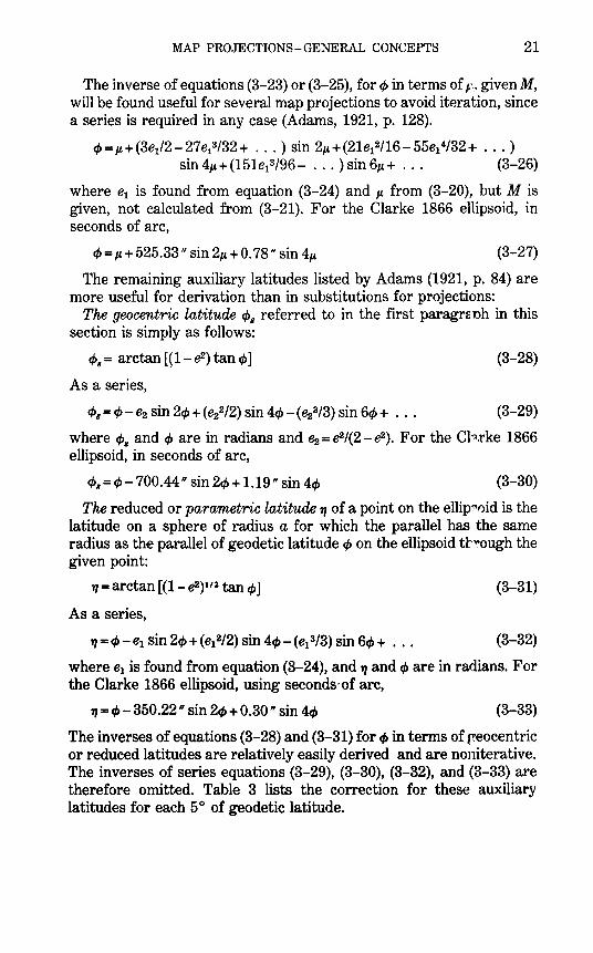
The inverse of equations (3-23) or (3-25), for cJ> in terms off· given M, will be found useful for several map projections to avoid iteration, since a series is required in any case (Adams, 1921, p. 128).
cJ> = !L+(3e1/2- 27e.3/32 + ... ) sin 2/L+ (21e12/16- 55e1
4/32 + ... ) sin 4/L+(151e1
3/96- ... ) sin 6/L+ • . . (3-26)
where e1 is found from equation (3-24) and IL from (3-20), but M is given, not calculated from (3-21). For the Clarke 1866 ellipsoid, in seconds of arc,
cJ> = IL + 525.33" sin 2/L + 0. 78" sin 4/L (3-27)
The remaining auxiliary latitudes listed by Adams (1921, p. 84) are more useful for derivation than in substitutions for projections:
The geocentric latitude c/>11
referred to in the first paragra oh in this section is simply as follows:
c/>11 = arctan [(1- e2) tan cJ>]
As a series,
c/>11 = cJ>- e2 sin 2cp +(e22/2) sin 4cp -(e2
3/3) sin 6cp + ...
(3-28)
(3-29)
where c/>11 and cJ> are in radians and e2 = e2/(2- e2). For the Cl'='.rke 1866 ellipsoid, in seconds of arc,
c/>11 =c/>-700.44" sin 2cp+ 1.19" sin 4cp (3-30)
The reduced or parametric latitude 7J of a point on the ellip<:'0id is the latitude on a sphere of radius a for which the parallel has the same radius as the parallel of geodetic latitude cJ> on the ellipsoid t:t~ough the given point:
7J =arctan [(1- e2)1' 2 tan cp] (3-31)
As a series,
(3-32)
where e1 is found from equation (3-24), and 7J and cJ> are in radians. For the Clarke 1866 ellipsoid, using seconds-of arc,
7J = t/>- 350.22" sin 2tJ> + 0.30" sin 4t/> (3-33)
The inverses of equations (3-28) and (3-31) for tJ> in terms of c-eocentric or reduced latitudes are relatively easily derived and are noniterative. The inverses of series equations (3-29), (3-30), (3-32), and (3-33) are therefore omitted. Table 3 lists the correction for these auxiliary latitudes for each 5° of geodetic latitude.
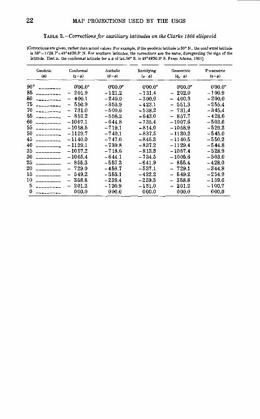
22 MAP PROJECTIONS USED BY THE USGS
TABLE 3.-Correctionsfor auxiliary latitudes on the Clarke 1866 eUiproid
[Corrections are given, rather than actual values. For example, if the geodetic latitude is 50° N., the conf'lrmallatitude is 50° -11'29. 7" = 49°48'30.3" N. For southern latitudes, the corrections are the same, disregarding the sign of the latitude. That is, the conformal latitude for a .p of lat. 50° S. is 49° 48'30.3" S. From Adams, 1921]
Geodetic Conformal Authalic Rectifying Geocentric Pwametric (</!) (x-.p) (tJ-.P) (p.-</J) (</!,-</!) (17-</!)
90° -------- 0'00.0" 0'00.0" 0'00.0" 0'00.0" 0'00.0" 85 --------- - 201.9 -121.2 -131.4 - 202.0 -100.9 80 --------- - 400.1 -240.0 -300.0 - 400.3 -200.0 75 --------- - 550.9 -353.9 -423.1 - 551.3 -255.4 70 --------- - 731.0 -500.6 -538.2 - 731.4 -345.4 65 --------- - 857.2 -558.2 -643.0 - 857.7 -428.6 60 --------- -1007.1 -644.8 -735.4 -1007.6 -503.6 55 --------- -1058.5 -719.1 -814.0 -1058.9 -529.3 50 --------- -1129.7 -740.1 -837.5 -1130.2 -545.0 45 --------- -1140.0 -747.0 -845.3 -1140.5 -550.2 40 --------- -1129.1 -739.8 -837.2 -1129.4 -544.8 35 --------- -1057.2 -718.6 -813.3 -1057.4 -528.9 30 --------- -1005.4 -644.1 -734.5 -1005.6 -503.0 25 --------- - 855.3 -557.3 -641.9 - 855.4 -428.0 20 --------- - 729.0 -459.7 -537.1 - 729.1 -344.8 15 --------- - 549.2 -353.1 -422.2 - 549.2 -254.9 10 --------- - 358.8 -239.4 -259.3 - 358.8 -159.6
5 --------- - 201.2 -120.9 -131.0 - 201.2 -100.7 0 --------- 000.0 000.0 000.0 000.0 000.0
4. SCALE VARIATION AND ANGULAR DISTORTION
Since no map projection maintains correct scale throughout, it is important to determine the extent to which it varies on a map. On a world map, qualitative distortion is evident to an eye familiar with maps, noting the extent to which landmasses are improperly size1 or out of shape, and the extent to which meridians and parallels do not intersect at right angles, or are not spaced uniformly along a given neridian or given parallel. On maps of countries or even of continents. distortion may not be evident to the eye, but becomes apparent upon careful measurement and analysis.
TISSOT'S INDICATRIX
In 1859 and 1881, Tissot published a classic analysis of the distortion which occurs on a map projection (Tissot, 1881; Adamr. 1919, p. 153-163; Maling, 1973, p. 64-67). The intersection of any t·vo lines on the Earth is represented on the flat map with an intersection at the same or a different angle. At almost every point on the Eartl', there is a right angle intersection of two lines in some direction (not n('~essarily a meridian and a parallel) which are also shown at right angles on the map. All the other intersections at that point on the Earth will not intersect at the same angle on the map, unless the map is conformal. The greatest deviation from the correct angle is called w, the maximum angular deformation. For a conformal map, w is zero.
Tissot showed this relationship graphically with a special ellipse of distortion called an indicatrix. An infinitely small circle on tbe Earth projects as an infinitely small, but perfect, ellipse on any map projection. If the projection is conformal, the ellipse is a circle, an ellipse of zero eccentricity. Otherwise, the ellipse has a major axis and minor axis which are directly related to the scale distortion and to the maximum angular deformation.
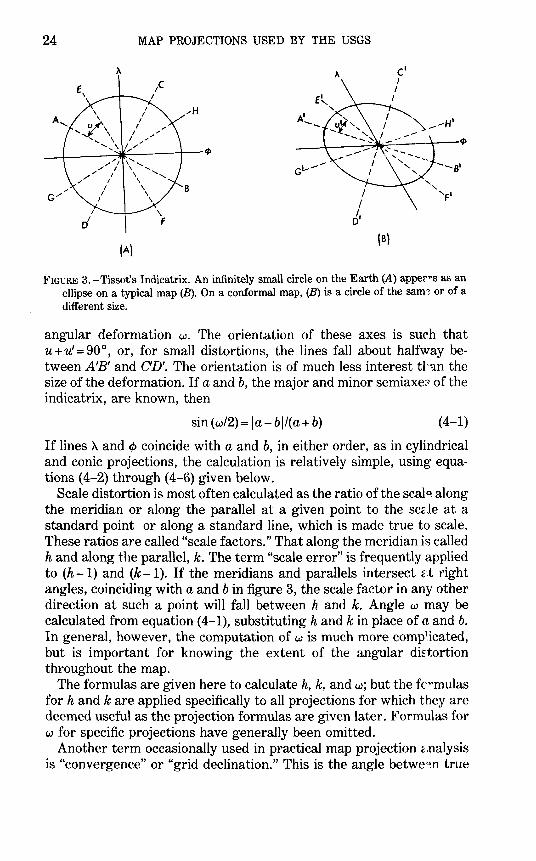
In figure 3, the left-hand drawing shows a circle repref'9nting the infinitely small circular element, crossed by a meridian >.. and parallel cJ>
on the Earth. The right-hand drawing shows this same element as it may appear on a typical map projection. For general purposes, the map is assumed to be neither conformal nor equal-area. The meridian and parallel may no longer intersect at right angles, but there is a pair of axes which intersect at right angles on both Earth (AB and CD) and map (A'B' and CD'). There is also a pair of axes which intersP.ct at right angles on the Earth (EF and GH), but at an angle on the map (E'F' and G'H') farthest from a right angle. The latter case has the maximum
23
24 MAP PROJECTIONS USED BY THE USGS
(A) (B)
FIGURE 3.-Tissot's Indicatrix. An infinitely small circle on the Earth (A) apper ... s as an ellipse on a typical map (B). On a conformal map, (B) is a circle of the sam~ or of a different size.
angular deformation w. The orientation of these axes is such that u + u' = 90 °, or, for small distortions, the lines fall about halfway between A'B' and C'D'. The orientation is of much less interest tb:1.n the size of the deformation. If a and b, the major and minor semiaxe;;: of the indicatrix, are known, then
sin{w/2)= la-bll(a+b) (4-1)
If lines A. and (j> coincide with a and b, in either order, as in cylindrical and conic projections, the calculation is relatively simple, using equations ( 4-2) through ( 4-6) given below.
Scale distortion is most often calculated as the ratio of the seal~ along the meridian or along the parallel at a given point to the sc2.le at a standard point or along a standard line, which is made true to scale. These ratios are called "scale factors." That along the meridian is called h and along the parallel, k. The term "scale error" is frequently applied to (h-1) and (k-1). If the meridians and parallels intersect 2'.t right angles, coinciding with a and b in figure 3, the scale factor in any other direction at such a point will fall between h and k. Angle w may be calculated from equation (4-1), substituting hand kin place of a and b. In general, however, the computation of w is much more comp1icated, but is important for knowing the extent of the angular di~tortion throughout the map.
The formulas are given here to calculate h, k, and w; but the fc:--mulas for h and k are applied specifically to all projections for which they are deemed useful as the projection formulas are given later. Formulas for w for specific projections have generally been omitted.
Another term occasionally used in practical map projection 2'.nalysis is "convergence" or "grid declination." This is the angle betwe~n true
MAP PROJECTIONS- GENERAL CONCEPTS 25
north and grid north (or direction of the Y axis). For regular cylindrical projections this is zero, for regular conic and polar azimuth~.l projections it is a simple function of longitude, and for other proja.ctions it may be determined from the projection formulas by calculus as the slope of the meridian (dyldx) at a given latitude. It is used primarily by surveyors for fieldwork with topographic maps. It has been d€cided not to discuss convergence further in this bulletin.
DISTORTION FOR PROJECTIONS OF THE SPHERE
The formulas for distortion are simplest when applied to regular cylindrical, conic (or conical), and polar azimuthal projections of the sphere. On each of these types of projections, scale is solely r. function of the latitude.
Given the formulas for rectangular coordinates x and y of any cylindrical projection as functions solely of longitude )1. and la.titude c/>, respectively,
h = dyi(Rdc/>) k = dxi(R cos ¢d)~.)
(4-2) (4-3)
Given the formulas for polar coordinates p and () of any cor ic projection as functions solely of¢ and )1., respectively, where n is the cone constant or ratio of 8 to (>..- )l.o),
h = - dpi(Rdc/>) k=npi(R cos¢)
(4-4) (4-5)
Given the formulas for polar coordinates p and 8 of any polar azimuthal projection as functions solely of cJ> and>.., respectiv~ly, equations (4-4) and (4-5) apply, with n equal to 1.0:
h= -dpi(Rdc/>) k= pi(R cos¢)
(4-4) (4-6)
Equations ( 4-4) and ( 4-6) may be adapted to any azimuth::tl projection centered on a point other than the pole. In this case h' is the scale factor in the direction of a straight line radiating from the center, and k' is the scale factor in a direction perpendicular to the radiatirg line, all at an angular distance c from the center:
h: = dpi(Rdc) k' = p/(R sin c)
(4-7) (4-8)
An analogous relationship applies to scale factors on oblique cylindrical and conic projections.
26 MAP PROJECTIONS USED BY THE USGS
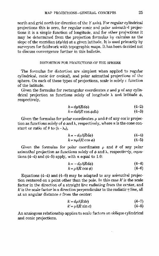
Transverse Mercator Projection
Lambert Conformal Conic Projection
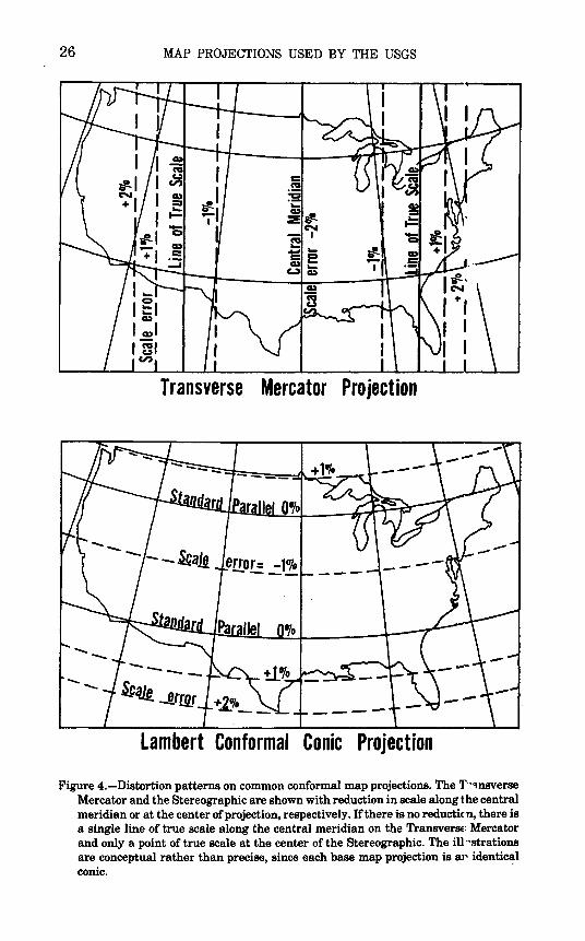
·Figure 4.-Distortion patterns on common conformal map projections. The 'f··"nsverse Mercator and the Stereographic are shown with reduction in scale along the central meridian or at the center of projection, respectively. If there is no reductkn, there is a single line of true scale along the central meridian on the TransversE: Mercator and only a point of true scale at the center of the Stereographic. The ill ··strations are conceptual rather than precise, since each base map projection is aP identic~l conic.
MAP PROJECTIONS-GENERAL CONCEPTS 27
Oblique Stereographic Projection
FIGURE 4.-Continued.
For any of the pairs of equations from (4-2) through (4-8), the maximum angular deformation w at any given point is calculated simply, as stated above,
sin 112w= lh-kll(h+k) (4-9)
where lh-kl signifies the absolute value of (h-k), or the positive value without regard to sign. For equations (4-7) and (4-8), h' and k' are used in (4-9) instead of hand k, respectively. In figure 4, distortion patterns are shown for three conformal projections of· the United States, choosing arbitrary lines of true scale.
For the general case, including all map projections of the s~here, rectangular coordinates x and y are often both functions of bot.h cf> and A, so they must be partially differentiated with respect to both cf> and A, holding A and¢, respectively, constant. Then,
h= (liR) [(ax/a¢)2 +(oyla¢)2)1 12
k = [1/(R cos ct> )] [(axlaA)2 + (ayloA)2JI' 2
a'= (h2 + k2 + 2hk sin 8') 112
b' = (h2 + k2- 2hk sin 8') 112
(4-10)
(4-11)
(4-12)
(4-13)
where cos 8' = [(ay/ocf>}(oyloA)+(ox/ocf>}(oxloA)]I(hk cos c/>) (4-14)
28 MAP PROJECTIONS USED BY THE USGS
(}'is the angle at which a given meridian and parallel intersect, and a' and b' are convenient terms. The maximum and minimum scale factors a and b, at a given point, may be calculated thus:
a= (a'+ b')/2 b=(a'- b')/2
Equation ( 4-1) simplifies as follows for the general case:
sin (w/2) = b'!a'
The areal scale factors:
s=hk sin 8'
For special cases:
(4-12a) (4-13a)
(4-1a)
(4-15)
(1) s=hk if meridians and parallels intersect at right angles (ll'=90°); (2) h = k and w = 0 if the map is conformal; (3) h= 1/k on an equal-area map if meridians and parallels intersect at right angles. 2
DISTORTION FOR PROJECTIONS OF THE ELLIPSOID
The derivation of the above formulas for the sphere utilizes the basic formulas for the length of a given spacing (usually 1° or 1 radian) along a given meridian or a given parallel. The following formulas give the length of a radian of latitude (Lq,) and of longitude (L.,..) for the sphere:
(4-16) (4-17)
where R is the radius of the sphere. For the length of 1 o of latitude or longitude, these values are multiplied by 1r/180.
The radius of curvature on a sphere is the same in all directions. On the ellipsoid, the radius of curvature varies at each point and in each direction along a given meridian, except at the poles. The radius of curvature R' in the plane of the meridian is calculated as follow~·:
(4-18)
The length of a radian of latitude is defined as the circumference of a circle of this radius, divided by 21r, or the radius itself. Thus,
Lq,=a{1-e2)/(1-e2 sin 2¢)3'
2 (4-19)
For the radius of curvature N of the ellipsoid in a plane perpendicular to the meridian and also perpendicular to a plane tangent to the surface,
' Mating (I ~173, p. 4!l-HJ) has helpful denvations of lht•se t•qualion;; 111 lt•ss <'ondt·n~l'd forms. Thl're :w.• ty pogTaphieal t>rrors 111 several of tlw t•quations 111 Mating·, hut tlll'st• ma,; he dl'lt•dl'd h,; follnll'lllg til<' dt•nvation dost{V.
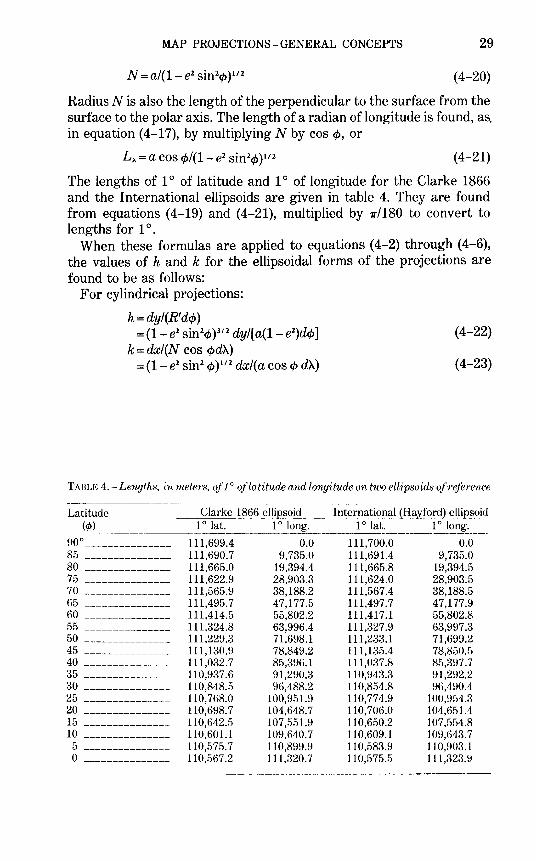
MAP PROJECTIONS-GENERAL CONCEPTS 29
(4-20)
Radius N is also the length of the perpendicular to the surface from the surface to the polar axis. The length of a radian of longitude is found, as. in equation ( 4-17), by multiplying N by cos cp, or
L-,.. =a cos cp/(1- e2 sin2cp )1'2 ( 4-21)
The lengths of 1 o of latitude and 1 o of longitude for the Clarke 1866 and the International ellipsoids are given in table 4. They are found from equations (4-19) and (4-21), multiplied by 1r/180 to convert to lengths for 1 °.
When these formulas are applied to equations ( 4-2) through ( 4-6), the values of h and k for the ellipsoidal forms of the projections are found to be as follows:
For cylindrical projections:
h = dyi(R' dcp) = (1- e2 sin2cp )3
'2 dy/[ a(1- e2)dcp]
k = dxi(N cos cpd'A) = (1- e2 sin2 c/>) 112 dx/(a cos cJ> d'A)
(4-22)
(4-23)
TABLE 4.-Lengths, in meters, ~~ll o of latitude and longitud-e on two ellipsoids oft·e..terent>e
Latitude __ Cl-,-ar_k_e_1_86_'6_e_ll_..._ip_so_id__ International (Hayford) ellipsoid _( __ c/J __ ) _______ 1 o lat. 1 o long. 1 o lat. 1 o long.
90°--------------- 111,699.4 0.0 111,700.0 0.0 85 --------------- 111,690.7 9,735.0 111,691.4 9,735.0 80 --------------- 111,665.0 19,394.4 111,665.8 19,394.5 75 --------------- 111,622.9 28,903.3 111,624.0 28,903.5 70 --------------- 111,565.9 38,188.2 111,567.4 38,188.5 65 --------------- 111,495.7 47,177.5 111,497.7 47,177.9 60 --------------- 111,414.5 55,802.2 111,417.1 55,802.8 55 --------------- 111,324.8 63,996.4 111,327.9 63,997.3 50 --------------- 111,229.3 71,698.1 111,233.1 71,699.2 45 --------------- 111,130.9 78,849.2 111,135.4 78,850.5 40 --------------- 111,032.7 85,396.1 111,037.8 85,397.7 35 --------------- 110,937.6 91,290.3 110,943.3 91,292.2 30 --------------- 110,848.5 96,488.2 110,854.8 96,490.4 25 --------------- 110,768.0 100,951.9 110,774.9 100,954.3 20 --------------- 110,698.7 104,648.7 110,706.0 104,651.4 15 --------------- 110,642.5 107,551.9 110,650.2 107,554.8 10 --------------- 110,601.1 109,640.7 110,609.1 109,643.7 5 --------------- 110,575.7 110,899.9 110,583.9 110,903.1 0 --------------- 110,567.2 111,320.7 110,575.5 111,323.9
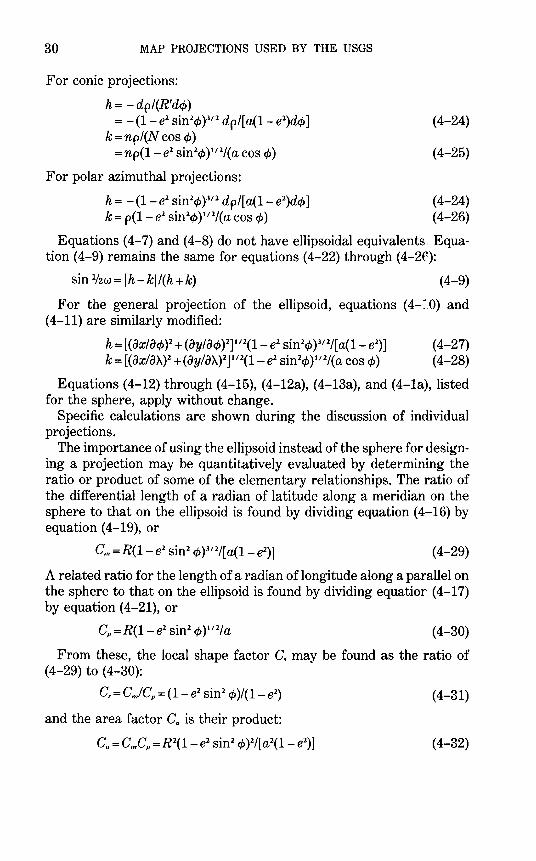
30 MAP PROJECTIONS USED BY THE USGS
For conic projections:
h= -dpi(R'd¢) = - (1- e2 sin2c/J }112 dp/[ a(1- e2)dc/J]
k = npi(N cos cf>) = np(1- e2 sin2¢)112/(a cos¢)
For polar azimuthal projections:
(4-24)
(4-25)
h = - (1- e2 sin2¢ )312 dpl[ a(1- e2)dc/J] ( 4-24) k = p(1- e2 sin2c/J )112
/( a cos cf>) ( 4-26)
Equations (4-7) and (4-8) do not have ellipsoidal equivalents- Equation ( 4-9) remains the same for equations ( 4-22) through ( 4-2f):
sin 1i2w= lh-kj/(h+k) (4-9)
For the general projection of the ellipsoid, equations (4-JO) and (4-11) are similarly modified:
h =[(ox/oct> )2 + (oy/ocf> )2)1' 2(1- e2 sin2¢ }112/[ a(1- e2
)] ( 4-27) k = [(oxlo>-.)2 + (oy/o>-.)2)1' 2(1- e2 sin2c/J) 1
'2/(a cos¢) (4-28)
Equations (4-12) through (4-15), (4-12a), (4-13a), and (4-1a), listed for the sphere, apply without change.
Specific calculations are shown during the discussion of individual projections.
The importance of using the ellipsoid instead of the sphere for designing a projection may be quantitatively evaluated by determining the ratio or product of some of the elementary relationships. The ratio of the differential length of a radian of latitude along a meridian on the sphere to that on the ellipsoid is found by dividing equation (4-16) by equation (4-19), or
(4-29)
A related ratio for the length of a radian of longitude along a parallel on the sphere to that on the ellipsoid is found by dividing equatior ( 4-17) by equation (4-21), or
(4-30)
From these, the local shape factor C.. may be found as the ratio of ( 4-29) to ( 4-30):
C..= Cm!C" = (1- e2 sin2 cf> )/(1- e2)
and the area factor C" is their product:
C" = CmCp =R2(1- e2 sin2 ct> )2/[ a 2(1- e2)]
(4-31)
(4-32)
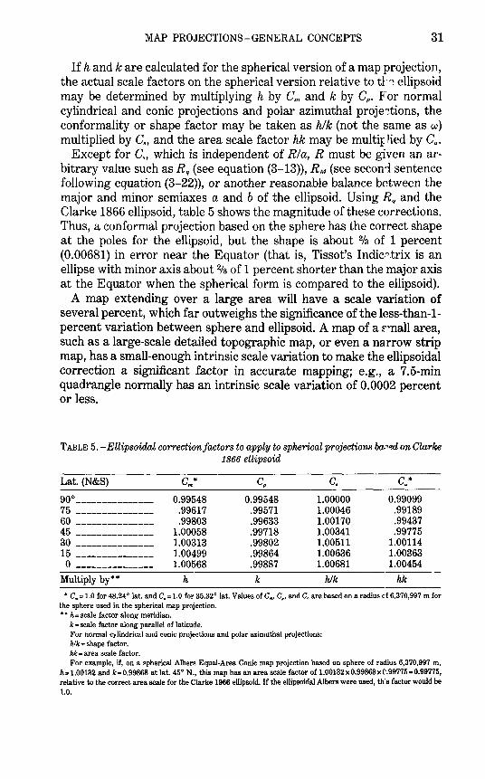
MAP PROJECTIONS-GENERAL CONCEPTS 31
If h and k are calculated for the spherical version of a map projection, the actual scale factors on the spherical version relative to tl:~ ellipsoid may be determined by multiplying h by Cm and k by Cp. For normal cylindrical and conic projections and polar azimuthal proje,~tions, the conformality or shape factor may be taken as hlk (not the same as w) multiplied by C.,, and the area scale factor hk may be multir 1ied by C".
Except for C., which is independent of Ria, R must be given an arbitrary value such as Rq (see equation (3-13)), RM (see seconi sentence following equation (3-22)), or another reasonable balance between the major and minor semiaxes a and b of the ellipsoid. Using Rq and the Clarke 1866 ellipsoid, table 5 shows the magnitude of these corrections. Thus, a conformal projection based on the sphere has the correct shape at the poles for the ellipsoid, but the shape is about 2/3 of 1 percent (0.00681) in error near the Equator (that is, Tissot's Indic"'.trix is an ellipse with minor axis about 2f3 of 1 percent shorter than the major axis at the Equator when the spherical form is compared to the ellipsoid).
A map extending over a large area will have a scale variation of several percent, which far outweighs the significance of the less-than-1-percent variation between sphere and ellipsoid. A map of a r'llall area, such as a large-scale detailed topographic map, or even a narrow strip map, has a small-enough intrinsic scale variation to make the ellipsoidal correction a significant factor in accurate mapping; e.g., a 7.5-min quadrangle normally has an intrinsic scale variation of 0.0002 percent or less.
TABLE 5.-Ellipsoidal correction factors to apply to spherical pro}ections ba.~qd on Clarke 1866 ellipsoid
Lat. (N&S) Cm* cp c. C,.* 90° _______________
0.99548 0.99548 1.00000 0.99099
75 --------------- .99617 .99571 1.00046 .99189
60 --------------- .99803 .99633 1.00170 .99437
45 --------------- 1.00058 .99718 1.00341 .99775
30 --------------- 1.00313 .99802 1.00511 1.00114
15 --------------- 1.00499 .99864 1.00636 1.00363
0 --------------- 1.00568 .99887 1.00681 1.00454
Multiply by** h k hlk hk
• C.,= 1.0 for 48.24° lat. and C.= 1.0 for 35.32° lat. Values of C.., C,, and C. are based on a radius of 6,370,997 m for the sphere used in the spherical map projection. • • h =scale factor along meridian.
k = scale factor along parallel of latitude. For normal cylindrical and conic projections and polar azimuthal projections: hlk = shape factor. hk=area scale factor. For example, if, on a spherical Albers Equal-Area Conic map projection based on sphere of radius 6,370,997 m,
h -1.00132 and k .. 0.99868 at lat. 45 o N ., this map has an area scale factor of 1.00132 x 0.99868 x (' .99775 • 0.99775, relative to the correct area scale for the Clarke 1966 ellipsoid. If the ellipsoidal Albers were used, th's factor would be 1.0.

5. TRANSFORMATION OF MAP GRATICULES
As discussed later, several map projections have been rrlapted to showing some part of the Earth for which the lines of true scr.le have an orientation or location different from that intended by the inve~tor of the basic projection. This is equivalent to moving or transfcrming the graticule of meridians and parallels on the Earth so that the "north pole" of the graticule assumes a position different from that of the true North Pole of the Earth. The projection for the sphere may be plotted using the original formulas or graphical construction, but applying them to the new graticule orientation. The actual meri iians and parallels may then be plotted by noting their relationship on the sphere to the new graticule, and landforms drawn with respect to the actual geographical coordinates as usual.
In effect, this procedure was used in the past in an often entirely graphical manner. It required considerable care to avoid cumulative errors resulting from the double plotting of graticules. With computers and programmable hand calculators, it now can be a relatively routine matter to calculate directly the rectangular coordinates of the actual graticule in the transformed positions or, with an automatic plotter, to obtain the transformed map directly from the computer.
The transformation most notably has been applied to the azimuthal and cylindrical projections, but in a few cases it has been used with conic, pseudocylindrical, and other projections. While it is fairly straightforward to apply a suitable transformation to the sphere, transformation is much more difficult on the ellipsoid because of the constantly changing curvature. Transformation has been appl:~d to the ellipsoid, however, in important cases under certain limitjng conditions.
If either true pole is at the center of an azimuthal map proj<'~tion, the projection is called the polar aspect. If a point on the Equator is made the center, the projection is called the equatorial or, less often, meridian or meridional aspect. If some other point is central, the projection is the oblique or, occasionally, horizon aspect.
For cylindrical and most other projections, such transform~tions are called transverse or oblique, depending on the angle of rotation. In transverse projections, the true poles of the Earth lie on the equator of the basic projection, and the poles of the projection lie on the Equator of the Earth. Therefore, one meridian of the true Earth lies along the equator of the basic projection. The Transverse Mercator projection is the best-known example and is related to the regular Mercator in this manner. For oblique cylindrical projections, the true poles of the Earth
33
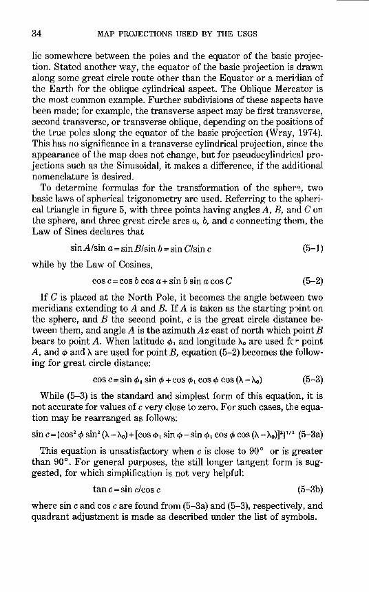
34 MAP PROJECTIONS USED BY THE USGS
lie somewhere between the poles and the equator of the basic projection. Stated another way, the equator of the basic projection is drawn along some great circle route other than the Equator or a meridian of the Earth for the oblique cylindrical aspect. The Oblique Mercator is the most common example. Further subdivisions of these aspects have been made; for example, the transverse aspect may be first transverse, second transverse, or transverse oblique, depending on the positions of the true poles along the equator of the basic projection (Wray, 1974). This has no significance in a transverse cylindrical projection, since the appearance of the map does not change, but for pseudocylindrical projections such as the Sinusoidal, it makes a difference, if the additional nomenclature is desired.
To determine formulas for the transformation of the spher~, two basic laws of spherical trigonometry are used. Referring to the spherical triangle in figure 5, with three points having angles A, B, and C on the sphere, and three great circle arcs a, b, and c connecting them, the Law of Sines declares that
sin A/sin a= sin B/sin b =sin C/sin c
while by the Law of Cosines,
cos c = cos b cos a+ sin b sin a cos C
(5-1)
(5-2)
If C is placed at the North Pole, it becomes the angle between two meridians extending to A and B. If A is taken as the starting p')int on the sphere, and B the second point, c is the great circle distance between them, and angle A is the azimuth Az east of north which point B bears to point A. When latitude cpt and longitude Ao are used fc r point A, and cp and }.. are used for point B, equation (5-2) becomes the following for great circle distance:
cos c =sin cpt sin cp +cos cpt cos cp cos(>-.- Ao) (5-3)
While (5-3) is the standard and simplest form of this equation, it is not accurate for values of c very close to zero. For such cases, the equation may be rearranged as follows:
sin c = (cos2 cp sin2 (>-.- >-.o) + [cos cpl sin cp- sin cp. cos cp cos(>-.- >-.o)]2) 112 (5-3a)
This equation is unsatisfactory when cis close to 90° or is greater than 90°. For general purposes, the still longer tangent form is suggested, for which simplification is not very helpful:
tan c =sin c/cos c (5-3b)
where sin c and cos care found from (5-3a) and (5-3), respectively, and quadrant adjustment is made as described under the list of symbols.
MAP PROJECTIONS-GENERAL CONCEPTS
Equation (5-1) becomes the following for the azimuth:
sin Az =sin (A.- 'Ao) cos <t>/sin c
or, with some rearrangement,
cosAz= [cos <1>1 sin <t>- sin <j> 1 cos <t> cos (A.- 'Ao)]/sin c
or, eliminating c,
35
(5-4)
(5-5)
tan Az =cos <t> sin (A.- 'Ao)/[cos <1>1 sin <t>- sin <1>1 cos <t> cos (A.- 'Ao)] (5-6)
Either of the three equations (5-4) through (5-6) may be used for the azimuth, depending on the form of equation preferred. Equation (5-6) is usually preferred, since it avoids the inaccuracies of finding an arcsin near 90° or an arccos near 0°. Quadrant adjustment as described under the list of symbols should be employed.
Applying these relationships to transformations, without showing some intermediate derivations, formulas (5-7) through (5·-10) are obtained. To place the North Pole of the sphere at a latitude a on a meridian {3 east of the central meridian ('A'= 0) of the basic projec+ion (see fig. 6), the transformed latitude <t>' and transformed longitude 'A' on the basic projection which correspond to latitude <t> and longit'1de 'A of the spherical Earth may be calculated as follows, letting the central meridian A.o correspond with 'A'= {3:
sin <t>' = sin a sin cp - cos a cos cp cos ('A- 'Ao) (5-7) sin ('A'- {3) =cos <t> sin ('A- }..0)/cos cp' (5-8)
or cos ('A'- {3) = [sin a cos cp cos ('A- 'Ao) +cos a sin cp ]/cos <t>' (5-9)
or tan ('A' - {3) = cos cp sin ('A- A.o)/[ sin a cos cp cos ('A- 'Ao)
+cos a sin¢] (5-10)
Equation (5-10) is generally preferable to (5-8) or (5-9) for the reasons stated after equation (5-6).
These are general formulas for the oblique transformation. (For azimuthal projections, {3 may always be taken as zero. Othe ... values of {3 merely have the effect of rotating the X and Y axes witho·1t changing the projection.)
The inverse forms of these equations are similar in app~arance. To find the geographic coordinates in terms of the transformed coordinates,
sin ¢ = sin a sin <t>' + cos a cos <t>' cos ('A' - {3) sin ('A- 'Ao) =cos <t>' sin ('A'- {3)/cos cp
or cos ('A- 'Ao) = [sin a cos cp' cos ('A'- {3)- cos a sin <t>1/ cos cp
or tan ('A- 'Ao) = cos <t>' sin ('A' - {3)/[ sin a cos <t>' cos ('A'- (i)
- cos a sin <t>']
(5-11) (5-12) (5-13)
(5-14)
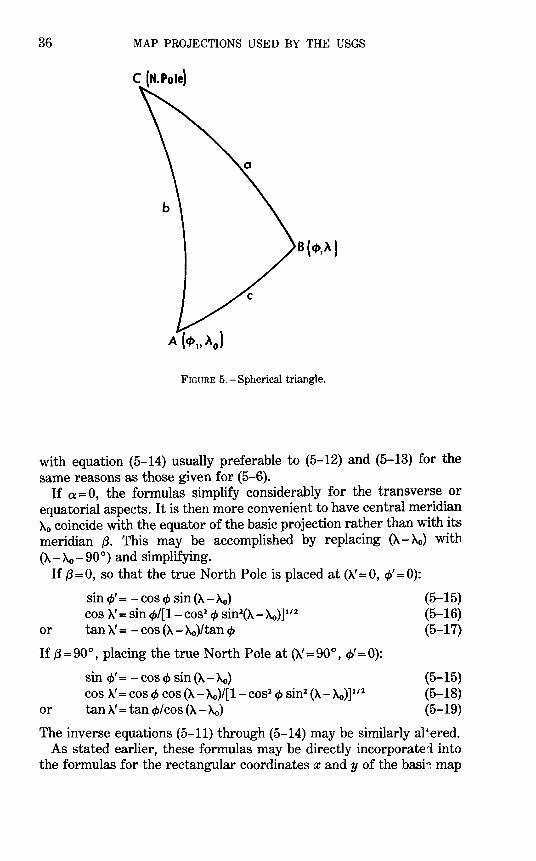
36 MAP PROJECTIONS USED BY THE USGS
C (N.Pole)
B(ct>,~)
FIGURE 5.- Spherical triangle.
with equation (5-14) usually preferable to (5-12) and (5-13) for the same reasons as those given for (5-6).
If a= 0, the formulas simplify considerably for the transverse or equatorial aspects. It is then more convenient to have central meridian Ao coincide with the equator of the basic projection rather than with its meridian {3. This may be accomplished by replacing (A- 'Ao) with (A- 'Ao- 90°) and simplifying.
If {3=0, so that the true North Pole is placed at (A'=O, c/>'=0):
or
sin cf>' = - cos cp sin (A- 'Ao) cos A'= sin cp/[1- cos2 cf> sin2(A- 'Ao)]112
tan A'= - cos (A- 'Ao)/tan cp
If {3 = 90°, placing the true North Pole at (A'= 90°, cp' = 0):
sin cf>' = - cos ¢ sin (A- 'Ao) cos A'= cos¢ cos (A- 'Ao)/[1- cos2 cp sin2 (A- 'Ao)] 1
'2
or tan A'= tan cp/cos (A- 'Ao)
(5-15) (5-16) (5-17)
(5-15) (5-18) (5-19)
The inverse equations (5-11) through (5-14) may be similarly al~ered. As stated earlier, these formulas may be directly incorporatei into
the formulas for the rectangular coordinates x and y of the basi~ map
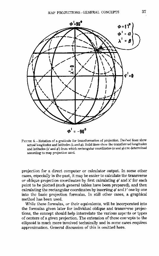
MAP PROJECTIONS- GENERAL CONCEPTS 37
4>1 = -900
FIGURE 6. -Rotation of a graticule for transformation of projection. Dashed lines show actual longitudes and latitudes (A. and 4> ). Solid lines show the transfon"'l.ed longitudes and latitudes (>..' and 4>) from which rectangular coordinates (x and y) ~.re determined according to map projection used.
projection for a direct computer or calculator output. In some other cases, especially in the past, it may be easier to calculate the transverse or oblique projection coordinates by first calculating cp' and >..' for each point to be plotted (such general tables have been prepared), and then calculating the rectangular coordinates by inserting cp' and)' one by one into the basic projection formulas. In still other cases, a graphical method has been used.
While these formulas, or their equivalents, will be incorporated into the formulas given later for individual oblique and transv,~rse projections, the concept should help interrelate the various aspe~ts or types of centers of a given projection. The extension of these con~epts to the ellipsoid is much more involved technically and in some· cases requires approximation. General discussion of this is omitted here.

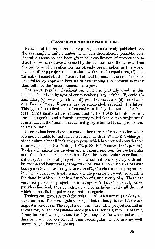
6. CLASSIFICATION OF MAP PROJECTIONS
Because of' the hundreds of map projections already published and the seemingly infinite number which are theoretically pcssible, considerable attention· has been given to classification of projections so that the user is not overwhelmed by the numbers and the variety. One obvious type of classification has already been implied in this work: division of map projections into those which are (1) equal-area, (2) conformal, (3) equidistant, (4) azimuthal, and (5) miscellaneour. This is an unsatisfactory approach because of overlapping and because so many then fall into the "miscellaneous" category.
The most popular classification, which is partially u~ed in this bulletin, is division by type of construction: (1) cylindrical, (2) conic, (3) azimuthal, (4) pseudocylindrical, (5) pseudoconical, and (6) miscellaneous. Each of these divisions may be subdivided, especially the latter. This type of classification is often easier to distinguish, but i~. is far from ideal. Since nearly all projections used by the USGS fall into the first three categories, and a fourth category called "space map projections" is introduced, the "miscellaneous" category is limited to two projections in this bulletin.
Interest has been shown in some other forms of classification which are more suitable for extensive treatises. In 1962, Waldo R. Tobler provided a simple but all-inclusive proposal which has aroused considerable interest (Tobler, 1962; Maling, 1973, p. 98-104; Maurer, 1935, p. v-vii). Tobler's classification involves eight categories, four for rectangular and four for polar coordinates. For the rectangular coordinates, category A includes all projections in which both x andy vary with both latitude cJ> and longitude A, category B includes all in which y varies with both cJ> and A while xis only a function of A, C includes those projections in which x varies with both cJ> and A while y varies only witb c/>, and D is for those in which xis only a function of A andy only of¢ .. There are very few published projections in category B, but Cis u~·ually called pseudocylindrical, D is cylindrical, and A includes nearly all the rest which do not fit the polar coordinate categories.
Tobler's categories A to D for polar coordinates are respectively the same as those for rectangular, except that radius p is rez.d for y and angle 0 is read for x. The regular conic and azimuthal projections fall into category D, and the pseudoconical (such as Bonne's) into C. Category A may have a few projections like A (rectangular) for whict· polar coordinates are more convenient than rectangular. There are no wellknown projections in B (polar).
39
40 MAP PROJECTIONS USED BY THE USGS
Hans Maurer's detailed map projection treatise of 1935 introduced a "Linnaean" classification with five families ("true-circular", "straightsymmetrical," "curved-symmetrical," "less regular," and "comb~nation grids," to quote a translation) subdivided into branches, subbrr.nches, classes, groups, and orders (Maurer, 1935). As Maling says, Maurer's system "is only useful to the advanced student of the subject," but Maurer attempts for map projections what Linnaeus, the Swedish botanist, accomplished for plants and animals in the eighteenth century (Maling, 1973, p. 98). Other approaches have been taken by Lee (1944) and by Goussinsky (1951).
The individual projections used by the USGS are discussed b8low.
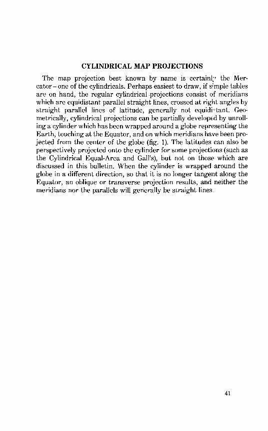
CYLINDRICAL MAP PROJECTIONS
The map projection best known by name is certainl:' the Mercator-one of the cylindricals. Perhaps easiest to draw, if s~mple tables are on hand, the regular cylindrical .projections consist of meridians which are equidistant parallel straight lines, crossed at right angles by straight parallel lines of latitude, generally not equidi"tant. Geometrically, cylindrical projections can be partially developE.d by unrolling a cylinder which has been wrapped around a globe representing the Earth, touching at the Equator, and on which meridians have been projected from the center of the globe (fig. 1). The latitudes can also be perspectively projected onto the cylinder for some projections (such as the Cylindrical Equal-Area and Gall's), but not on those which are discussed in this bulletin. When the cylinder is wrapped around the globe in a different direction, so that it is no longer tangent along the Equator, an oblique or transverse projection results, and neither the meridians nor the parallels will generally be straight lines.
41

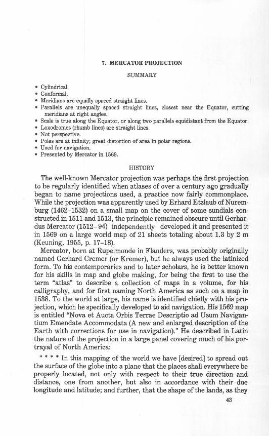
• Cylindrical. • Conformal.
7. MERCATOR PROJECTION
SUMMARY
• Meridians are equally spaced straight lines. • Parallels are unequally spaced straight lines, closest near the Equator, cutting
meridians at right angles. • Scale is true along the Equator, or along two parallels equidistant from the Equator. • Loxodromes (rhumb lines) are straight lines. • Not perspective. • Poles are at infinity; great distortion of area in polar regions. • Used for navigation. • Presented by Mercator in 1569.
HISTORY
The well-known Mercator projection was perhaps the first projection to be regularly identified when atlases of over a century ago gradually began to name projections used, a practice now fairly commonplace. While the projection was apparently used by Erhard Etzlaub of Nuremburg (1462-1532) on a small map on the cover of some sundials constructed in 1511 and 1513, the principle remained obscure until Gerhardus Mercator (1512- 94) independently developed it and presented it in 1569 on a large world map of 21 sheets totaling about 1.3 by 2 m (Keuning, 1955, p. 17 -18).
Mercator, born at Rupelmonde in Flander~, was probably originally named Gerhard Cremer (or Kremer), but he always used the latinized form. To his contemporaries and to later scholars, he is better known for his skills in map and globe making, for being the first to use the term "atlas" to describe a collection of maps in a volume, for his calligraphy, and for first naming North America as such on a map in 1538. To the world at large, his name is identified chiefly with his projection, which he specifically developed to aid navigation. His 1569 map is entitled "Nova et Aucta Orbis Terrae Descriptio ad Usum Navigantium Emendate Accommodata (A new and enlarged description of the Earth with corrections for use in navigation)." He described in Latin the nature of the projection in a large panel covering much of his portrayal of North America:
" * * * In this mapping of the world we have [desired] to spread out the surface of the globe into a plane that the places shall everywhere be properly located, not only with respect to their true direction and distance, one from another, but also in accordance with their due longitude and latitude; and further, that the shape of the lands, as they
43
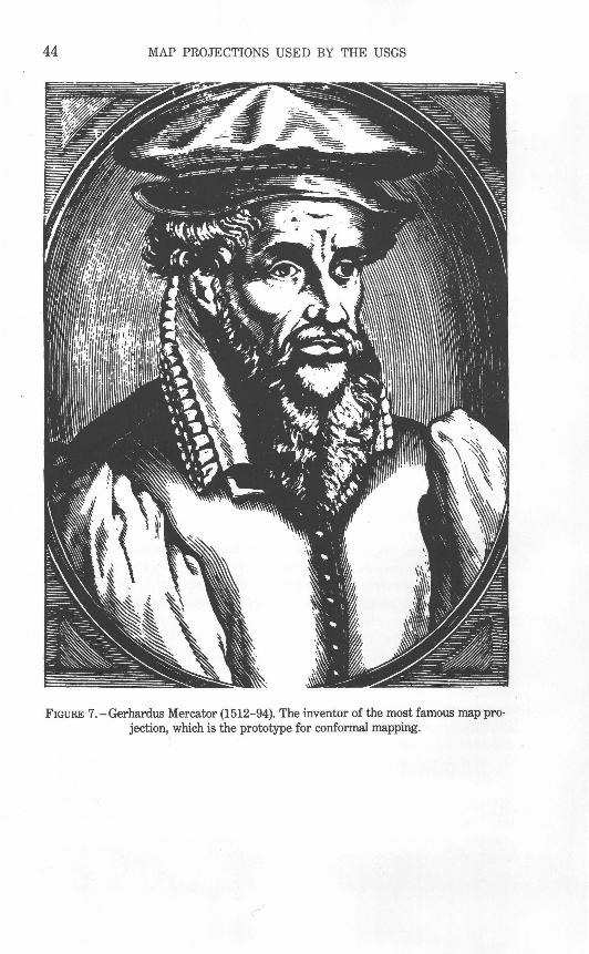
44 MAP PROJECTIONS USED BY THE USGS
FIGURE 7.-Gerhardus Mercator (1512-94). The inventor of the most famous map projection, which is the prototype for conformal mapping.
I
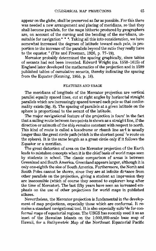
CYLINDRICAL MAP PROJECTIONS 45
appear on the globe, shall be preserved as far as possible. For this there was needed a new arrangement and placing of meridians, so that they shall become parallels, for the maps hitherto produced by geographers are, on account of the curving and the bending of the me~idians, unsuitable for navigation* * *. Taking all this into consideration, we have somewhat increased the degrees of latitude toward each pole, in proportion to the increase of the parallels beyond the ratio they really have to the equator." (Fite and Freeman, 1926, p. 77-78).
Mercator probably determined the spacing graphically, since tables of secants had not been invented. Edward Wright (ca. 15.58-1615) of England later developed the mathematics of the projection and in 1599 published tables of cumulative secants, thereby indicating the spacing from the Equator (Keuning, 1955, p. 18).
FEATURES AND USAGE
The meridians of longitude of the Mercator projection are vertical parallel equally spaced lines, cut at right angles by horizontal straight parallels which are increasingly spaced toward each pole so that conformality exists (fig. 8). The spacing of parallels at a given latitude on the sphere is proportional to the secant of the latitude.
The major navigational feature of the projection is founcl in the fact that a sailing route between two points is shown as a straight line, if the direction or azimuth of the ship remains constant with respect to north. This kind of route is called a loxodrome or rhumb line ani is usually longer than the great circle path (which is the shortest possi'"'1e route on the sphere). It is the same length as a great circle only if it follows the Equator or a meridian.
The great distortion of area on the Mercator projection cf the Earth leads to mistaken concepts when it is the chief basis of world maps seen by students in school. The classic comparison of areas is between Greenland and South America. Greenland appears larger, although it is only one-eighth the size of South America. Furthermore, theN orth and South Poles cannot be shown, since they are at infinite dirt,ance from other parallels on the projection, giving a student an impr~ssion they are inaccessible (which of course they seemed to explorer~ long after the time of Mercator). The last fifty years have seen an increased emphasis on the use of other projections for world maps in published atlases.
Nevertheless, the Mercator projection is fundamental in the development of map projections, especially those which are conformal. It remains a standard navigational tool. It is also especially suitrl:lle for conformal maps of equatorial regions. The USGS has recently used it as an inset of the Hawaiian Islands on the 1:500,000-scale base map of Hawaii, for a Bathymetric Map of the Northeast Equatorial Pacific
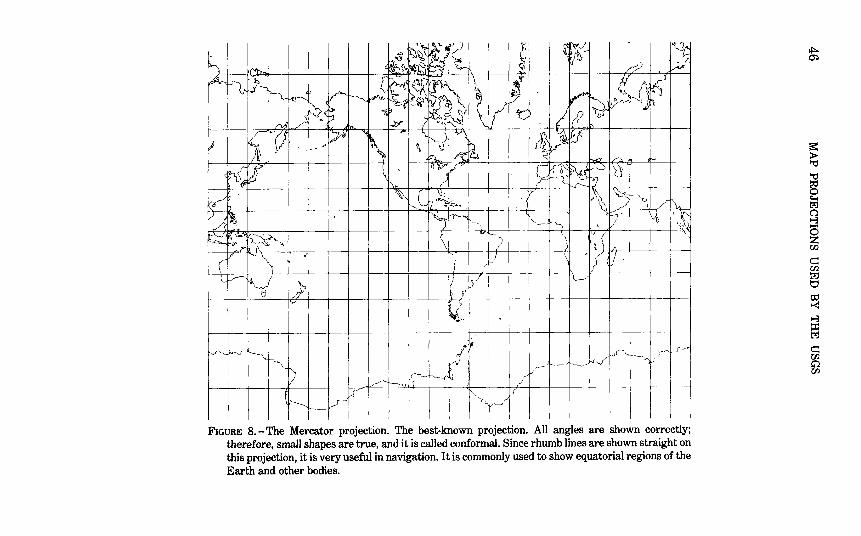
-~~~:· r( ~ ~~ '\..l
b;§ll ~~ >'~>{ \\~··
h lf"h ... f<J/i. ,....,~ '-, ~ l-J
~ hr v- J N ~ ~ \ ~ « W] ~ 'l__ p v-~ ~ ~ ~ ~ ~
R~ ~ [( ~ ~ ~
~ -z t / lrf_ l c
>rvj /-"' ~ .... ..y Pof
I ~ ~v v' l~ p \. N ;,.;\ a~ l) v
•' ' ~ ~ ~ "\ ><'"'T ,-,, f-.
~~ w \ ' IU~I'""
~ v.-'a~ M ~ lu
~h / ~ I'-. tJ v ~ ~~
\) .. 'V )\\ ~"-:; r,l ~~ ,c._ . < . ../ ~/ -~
) -lt ~ ~ t 'l; h' ~D ·~£ ,/( ....... \ '--,~ t'--1 I /
·'-1 ~--.:..'<: ~ P. •. ..,_ ~ f-\ I~ ( ~ "\:
~- ,.,.. \ )
r ~
( v '-.J\ ·r (j \ '( )·
~ I} t~ ~--./ //);; ~{ ? L--·
Q ---
y
~- ' -----
:-v~ ~ ~ "/~~ rr'" ._____,~ _,J~---_J~·r-:
"--, I·0/ I
) ·~~ ---------<';) J----
~~ ~ j'
t------ ~ ·,,_?..,._ / - ,.r I
,.r-./
I I I
FIGURE 8. -The Mercator projection. The best-known projection. All angles are shown correctly; therefore, small shapes are true, and it is called conformal. Since rhumb lines are shown straight on this projection, it is very useful in navigation. It is commonly used to show equatorial regions of the Earth and other bodies.
~ (j.)
s:: ~ ;g 8 t:z::l (i 1-3 0 z 00
c::: 00 l?=j t:l to t-< 1-3 ::X:: l?=j
c::: u; c;':l 00
CYLINDRICAL MAP PROJECTIONS 47
Ocean (although the projection is not stated) and for a Tectonic Map of the Indonesia region, the latter two both in 1978 and at a scale of 1:5,000,000.
The first detailed map of an entire planet other than the Earth was issued in 1972 at a scale of 1:25,000,000 by the USGS Center of Astrogeology, Flagstaff, Ariz., following imaging of Mars by Mariner 9. Maps of Mars at other scales have followed. The mapping of the planet Mercury followed the flybys of Mariner 10 in 1974. Beginning in the late 1960's, geology of the visible side of the Moon was rna oped by the USGS in quadrangle fashion at a scale of 1:1,000,000. The four Galilean satellites of Jupiter and several satellites of Saturn are be.ing mapped following the Voyager missions of 1979-81. For all these bodies, the Mercator projection has been used to map equatorial p1rtions, but coverage extends in some cases to lats. 65° N. and S. (Se~ table 6.)
The cloudy atmosphere of Venus, circled by the Pionee"' Venus Orbiter beginning in late 1978, is delaying more precise mapping of that planet, but the Mercator projection alone has been us~d to show altitudes based on radar reflectivity over about 93 percent of the surface.
FORMULAS FOR THE SPHERE
There is no suitable geometrical construction of the Mercator projection. For the sphere, the formulas for rectangular coordinates are as follows:
or
X=R ('A-'Ao) y = R In tan ( -rrl 4 + cJ>/2) y=R arctanh (sin c/>)
(7-1) (7-2)
(7-2a)
where R is the radius of the sphere at the scale of the mao as drawn, and cJ> and}.. are given in radians. The X axis lies along the Equator, x increasing easterly. The Y axis lies along the central meridian 'Ao, yincreasing northerly. If ('A- 'Ao) lies outside the range ± 180°, 360° should be added or subtracted so it will fall inside the range. To ur~ cJ> and }.. in degrees,
or
X= -rrR ('A 0 - 'Ao}/180° y=R In tan (45° +c/> 0 /2) y=R arctanh (sin c/>)
(7-la) (7-2b) (7-2c)
Equations (7-2a) and (7-2c) may be more convenient to use than (7-2) or (7-2b), if hyperbolic functions are standard to the computer or calculator. Note that if cJ> is ± -rr/2 or ± 90°, y is infinite. For scale factors, application of equations (4-2), (4-3), and (4-9) to (7-1) and (7-2) or
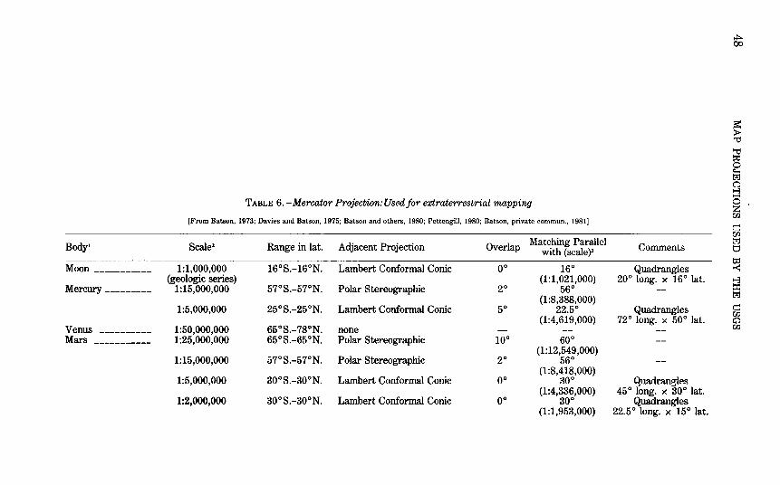
TABLE 6.-Mercator Projection: Used for extraterrestrial mapping
[From Batson, 1973; Davies and Batson, 1975; Batson and others, 1980; Pettengill, 1980; Batson, private commun., 1981]
Body1 Scale2 Range in lat. Adjacent Projection Overlap Matching Parallel with (scale)3
Moon ----------- 1:1,000,000 16°S.-16°N. Lambert Conformal Conic oo 16° (geologic series) (1:1,021,000)
Mercury--------- 1:15,000,000 57°S.-57°N. Polar Stereographic 20 56° (1:8,388,000)
1:5,000,000 25°S.-25°N. Lambert Conformal Conic 50 22.5° (1:4,619,000)
Venus ---------- 1:50,000,000 65°S.-78°N. none -- --Mars ----------- 1:25,000,000 65°S.-65°N. Polar Stereographic 100 60°
(1:12,549,000) 1:15,000,000 57°S.-57°N. Polar Stereographic 20 56°
(1:8,418,000) 1:5,000,000 30°S.-30°N. Lambert Conformal Conic oo B0°
1:2,000,000 30°S.-30°N. Lambert Conformal Conic (1:4,336,000) oo 30° (1:1,953,000)
Comments
Quadrangles 20° long. x 16° lat.
Quadrangles 72° long. x 50° lat.
Quadrangles 45 ° long. x 30° lat.
Quadrangles 22.5° long. x 15° lat.
~ 00
~ > "d
"d
~ ~ t?=.:l 0 ~
~ 00
c:: 00 t?=.:l t:::' ttl ~
~ t?=.:l
c::: 00 C":l 00
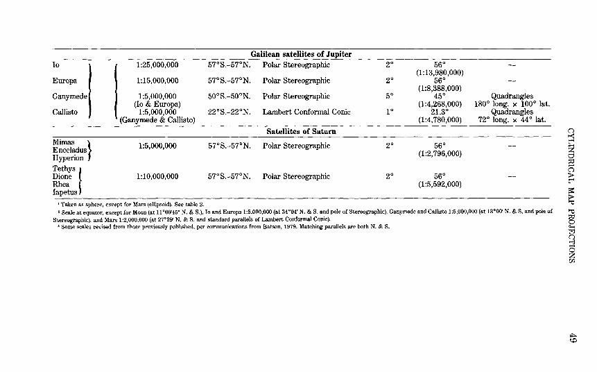
Galilean satellites of Jupiter Io 1:25,000,000 57°S.-57°N. Polar Stereographic 20 56°
(1:13,980,000) Europa 1:15,000,000 57°S.-57°N. Polar Stereographic 20 56°
(1:8,388,000) Ganymede 1:5,000,000 50°S.-50°N. Polar Stereographic 50 45° Quadrangles
(lo & Europa) (1:4,268,000) 180° long. x 100° lat. Callisto 1:5,000,000 22°S.-22°N. Lambert Conformal Conic 10 21.3° Quadrangles
(Ganymede & Callisto) (1:4, 780 ,000) 72° long. x 44 ° lat.
Satellites of Saturn
Mimas } 1:5,000,000 57°S.-57°N. Polar Stereographic 20 56° Enceladus Hyperion (1:2,796,000)
Tethys I Dione 1:10,000,000 57°S.-57°N. Polar Stereographic 20 56° Rhea (1:5,592,000) Iapetus
• Taken as sphere, except for Mars (ellipsoid). See table 2. 2 Scale at equator, except for Moon (at 11 °00'45" N. & S.), Io and Europa 1:5,000,000 (at 34°04' N. & S. and pole of Stereographic), Ganymede and Callisto 1:5,000,000 (at 13°00' N. & S. and pole of
Stereographic), and Mars 1:2,000,000 (at 27°29' N. & S. and standard parallels of Lambert Conformal Conic). 3 Some scales revised from those previously published, per communications from Batson, 1979. Matching parallels are both N. & S.
0 to< t"" z d ~ -0 > t""
s= > '"1:l
'"1:l
~ ~ l?j 0 1-3 -0 z rn
~ ~
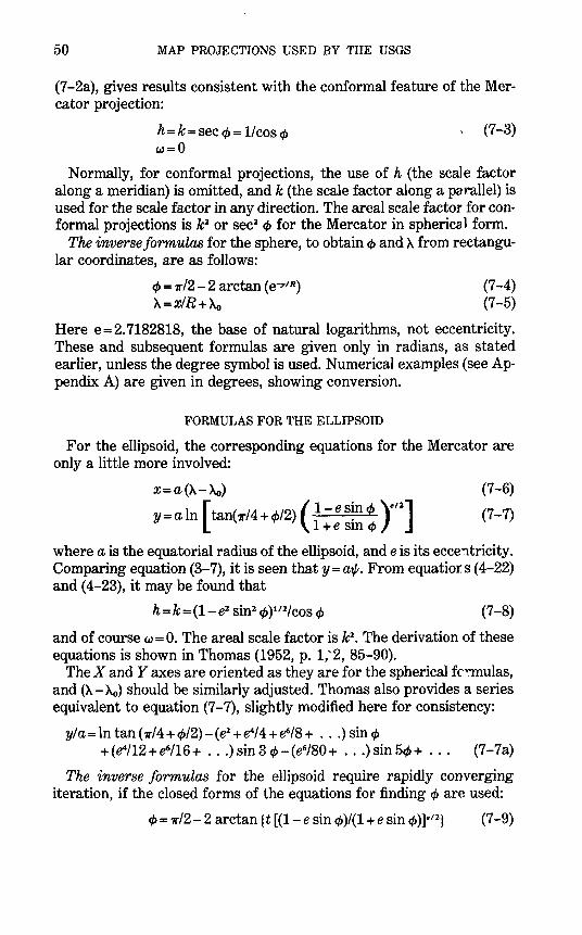
50 MAP PROJECTIONS USED BY THE USGS
(7 -2a), gives results consistent with the conformal feature of the Mercator projection:
h = k = sec cf> = 1/ cos cf> w=O
(7-3)
Normally, for conformal projections, the use of h (the scale factor along a meridian) is omitted, and k (the scale factor along a parallel) is used for the scale factor in any direction. The areal scale factor for conformal projections is k2 or sec2 q, for the Mercator in spherical form.
The inverse formulas for the sphere, to obtain cf> and 'A from rectangular coordinates, are as follows:
cf> = 1rl2- 2 arctan ( e-yl R) 'A=xiR +'Ao
(7-4) (7-5)
Here e = 2. 7182818, the base of natural logarithms, not eccentricity. These and subsequent formulas are given only in radians, as stated earlier, unless the degree symbol is used. Numerical examples (see Appendix A) are given in degrees, showing conversion.
FORMULAS FOR THE ELLIPSOID
For the ellipsoid, the corresponding equations for the Mercator are only a little more involved:
X=a('A-'Ao) (7-6)
y = a In [tan( 1rl 4 + q,/2) ( i -e s~n P )e'l] (7 -7) +e sin q,
where a is the equatorial radius of the ellipsoid, and e is its ecce--ttricity. Comparing equation (3-7), it is seen that y= a,P. From equatiors (4-22) and ( 4-23), it may be found that
(7-8)
and of course w = 0. The areal scale factor is k2• The derivation of these
equations is shown in Thomas (1952, p. 1,'2, 85-90). The X and Y axes are oriented as they are for the spherical fc~mulas,
and ('A- 'Ao) should be similarly adjusted. Thomas also provides a series equivalent to equation (7 -7), slightly modified here for consistency:
yla= In tan (7r/4+ ¢/2)- (e2 + e4/4 + e6/8 + ... ) sin q, +(e4/12+e6/16+ ... ) sin 3 ¢-(e6/80+ ... ) sin 5</>+ . . . (7-7a)
The inverse formulas for the ellipsoid require rapidly converging iteration, if the closed forms of the equations for finding <1> are used:
</>= 1rl2-2 arctan (t [(1-e sin <t>)/(1+e sin <t>)]e'2 } (7-9)
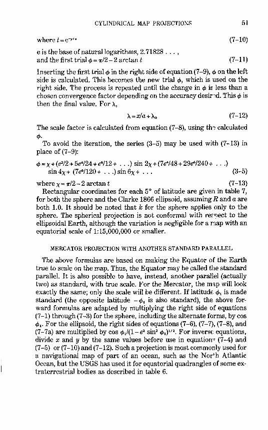
CYLINDRICAL MAP PROJECTIONS
where t = e-yta
e is the base of natural logarithms, 2. 71828 ... , and the first trial c1> = 1r/2- 2 arctan t
51
(7-10)
(7-11)
Inserting the first trial c1> in the right side of equation (7 -9), c1> on the left side is calculated. This becomes the new trial cj>, which is used on the right side. The process is repeated until the change in c1> is less than a chosen convergence factor depending on the accuracy desir~d. This c1> is then the final value. For A,
(7-12)
The scale factor is calculated from equation (7 -8), using th~ calculated cj>.
To avoid the iteration, the series (3-5) may be used with (7 -13) in place of (7-9):
ct>=x+(e2/2+5e4/24+e6/l2+ ... ) sin 2x+(7e4/48+29e6/240+ ... ) sin 4x + (7 e6/l20 + ... ) sin 6x + . . . (3-5)
where x = 1r/2- 2 arctan t (7 -13) Rectangular coordinates for each 5° of latitude are given in table 7,
for both the sphere and the Clarke 1866 ellipsoid, assuming R and a are both 1.0. It should be noted that k for the sphere applies only to the sphere. The spherical projection is not conformal with rer'1ect to the ellipsoidal Earth, although the variation is negligible for a nap with an equatorial scale of 1:15,000,000 or smaller.
MERCATOR PROJECTION WITH ANOTHER STANDARD PARALLEL
The above formulas are based on making the Equator of the Earth true to scale on the map. Thus, the Equator may be called the standard parallel. It is also possible to have, instead, another parallel (actually two) as standard, with true scale. For the Mercator, the m.::tp will look exactly the same; only the scale will be different. If latitudE: cj> 1 is made standard (the opposite latitude - cj> 1 is also standard), the above forward formulas are adapted by multiplying the right side of equations (7-1) through (7-3) for the sphere, including the alternate forms, by cos cj> 1 • For the ellipsoid, the right sides of equations (7-6}, (7-7}, (7-8}, and (7-7a) are multiplied by cos cj> 1/(l-e2 sin2 cj> 1}
112• For inversE: equations,
divide x andy by the same values before use in equation~ (7-4) and (7-5) or (7-10) and (7-12). Such a projection is most commonly used for a navigational map of part of an ocean, such as the North Atlantic Ocean, but the USGS has used it for equatorial quadrangles of some extraterrestrial bodies as described in table 6.
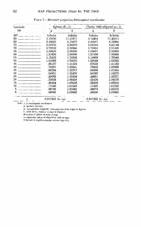
52 MAP PROJECTIONS USED BY THE USGS
TABLE 7. -Me-rcator p·rojection:Rectangu.la-r coo-rdinates
Latitude S_ehere (R = 1) Clarke 1866 elli_esoid {a= 1} (cp) y
90o _______________ Infinite
85 --------------- 3.13130 80 --------------- 2.43625 75 --------------- 2.02759 70 --------------- 1.73542 65 --------------- 1.50645 60 --------------- 1.31696 55 --------------- 1.15423 50 --------------- 1.01068 45 --------------- .88137 40 --------------- .76291 35 --------------- .65284 30 --------------- .54931 25 --------------- .45088 20 --------------- .35638 15 --------------- .26484 10 --------------- .17543
5 --------------- .08738 0 --------------- .00000
X 0.017453 (>.->.o)
Note: x, y =rectangular coordinates. </>=geodetic latitude.
k
Infinite 11.47371 5.75877 3.86370 2.92380 2.36620 2.00000 1.74345 1.55572 1.41421 1.30541 1.22077 1.15470 1.10338 1.06418 1.03528 1.01543 1.00382 1.00000
(>.- A0 )= geodetic longitude, measured east from origin in degrees. k= scale factor, relative to scale at Equator. R =radius of sphere at scale of map. a.= equatorial radius of ellipsoid at scale of map. If latitude is negative (south), reverse sign of y.
y k
Infinite Irfinite 3.12454 11.43511 2.42957 5.73984 2.02104 3.85148 1.72904 2.91505 1.50031 2.35961 1.31109 1.99492 1.14868 1.73948 1.00549 1.55263
.87658 1.41182
.75855 1.30358
.64895 1.21941
.54592 1.15372
.44801 1.10271
.35406 1.06376
.26309 1.03504
.17425 1.01532
.08679 1.00379
.00000 1.00000
0.017453 (>.->.o)
8. TRANSVERSE MERCATOR PROJECTION
SUMMARY
• Cylindrical (transverse). • Conformal. • Central meridian, each meridian 90° from central meridian, and Equator are
straight lines. • Other meridians and parallels are complex curves. • Scale is true along central meridian, or along two straight lines equidistant from and
parallel to central meridian. (These lines are only approximately straight for the ellipsoid.)
• Scale becomes infinite 90° from central meridian. • Used extensively for quadrangle maps at scales from 1:24,000 to 1:250,000. • Presented by Lambert in 1772.
HISTORY
Since the regular Mercator projection has little error close to the Equator (the scale 10° away is only 1.5 percent larger than the scale at the Equator), it has been found very useful in the transverse form, with the equator of the projection rotated 90° to coincide with the desired central meridian. This is equivalent to wrapping the cylinder around a sphere or ellipsoid representing the Earth so that it touches the central meridian throughout its length, instead of following the Equator of the Earth. The central meridian can then be made true to scale, no matter how far north and south the map extends, and regions near it are mapped with low distortion. Like the regular Mercator, the map is conformal.
The Transverse Mercator projection in its spherical form was invented by the prolific Alsatian mathematician and cartographer Johann Heinrich Lambert (1728-77). It was the third of six new projections which he described in 1772 in his classic Beitriige (Lambert, 1772). At the same ti:rpe, he also described what are now called the Lambert Conformal Conic and the Lambert Azimuthal Equal-Area, both of which will be discussed subsequently; others are omitted here. He described the Transverse Mercator as a conformal adaptation of the Sinusoidal projection, then commonly in use (Lambert, 1772, p. 57-58). Lambert's derivation was followed with a table of coordinates and a map of the Americas drawn according to the projection.
Little use has been made of the Transverse Mercator for single maps of continental areas. While Lambert only indirectly discussed its ellipsoidal form, mathematician Carl Friedrich Gauss (1777 -1855) analyzed it further in 1822, and L. Kruger published studies in 1912 and 1919 providing formulas suitable for calculation relative to the ellipsoid. It is,
53
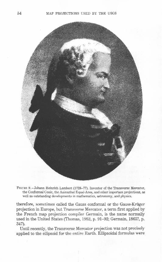
54 MAP PROJECTIONS USED BY THE USGS
FIGURE 9.-Johann Heinrich Lambert (1728-77). Inventor of the Transverse Mercator, the Conformal Conic, the Azimuthal Equal-Area, and other important projections, as well as outstanding developments in mathematics, astronomy, and physics.
therefore, sometimes called the Gauss conformal or the Gauss-Kruger projection in Europe, but Transverse Mercator, a term first applied by the French map projection compiler Germain, is the name normally used in the United States (Thomas, 1952, p. 91-92; Germain, 1865?, p. 347).
Until recently, the Transverse Mercator projection was not precisely applied to the ellipsoid for the entire Earth. Ellipsoidal formulas were
CYLINDRICAL MAP PROJECTIONS 55
limited to series for relatively narrow bands of about ±4 ° longitude. ln 1945, E. H. Thompson, (and in 1962, L. P. Lee) presented exact or closed formulas permitting calculation of coordinates for the full ellipsoid, although elliptic functions, and therefore length:r series, numericalintegrations,and (or) iterations, are involved (Lee, 1976, p. 92-101; Snyder, 1979a, p. 73; Dozier, 1980).
The formulas for the complete ellipsoid are interesting acad~mically, but they are practical only within a band between 4 o of lon~tude and some 10° to 15° of arc distance on either side of the central meridian, because of the much more significant scale errors fundamental to any projection covering a larger area.
FEATURES
The meridians and parallels of the Transverse Mercato:-- are no longer the straight lines they are on the regular Mercator, except for the Earth's Equator, the central meridian, and each meridian 90° away from the central meridian. Other meridians ctnd parallels are complex curves.
The spherical form is conformal, as is the parent projection, and scale error is only a function of the distance from the central meridian, just as it is only a function of the distance from the Equator on th~ regular Mercator. The ellipsoidal form is also exactly conformal, but its scale error is slightly affected by factors other than the distance al -:me from the central meridian (Lee, 1976, p. 98).
The scale along the central meridian may be made true to scale, or deliberately reduced to a slightly smaller constant scale so that the mean scale of the entire map is more nearly correct. There are also forms of the ellipsoidal Transverse Mercator on which the central meridian is not held at a constant scale, but these forms are not used in practice (Lee, 1976, p. 100-101). If the central meridian is mal)ped at a reduced scale, two straight lines parallel to it and equally spa ~ed from it, one on either side, become true to scale on the sphere. Tr~se lines are not perfectly straight on the ellipsoidal form.
With the scale along the central meridian remaining constant, the Transverse Mercator is an excellent projection for lands extending predominantly north and south.
USAGE
The Transverse Mercator projection (spherical or ellipsoidal) was not described by Close and Clarke in their generally detailed article in the 1911 Encyclopaedia Britannica because it was "seldom used" (Close and Clarke, 1911, p. 663). Deetz and Adams (1934) favorably referred to it several times, but as a slightly used projection.
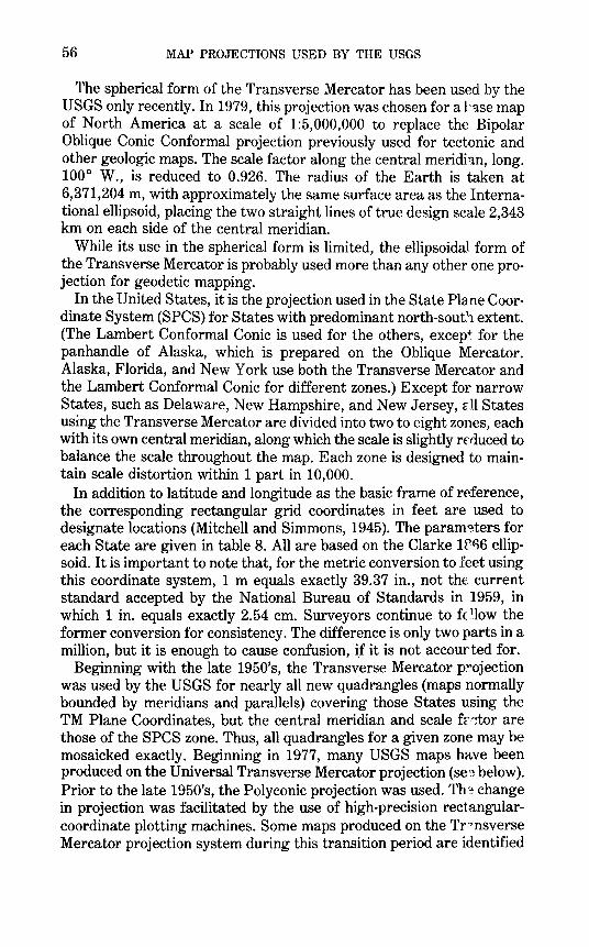
56 MAP PROJECTIONS USED BY THE USGS
The spherical form of the Transverse Mercator has been used by the USGS only recently. In 1979, this projection was chosen for a 1'-:tse map of North America at a scale of 1:5,000,000 to replace the Bipolar Oblique Conic Conformal projection previously used for tectonic and other geologic maps. The scale factor along the central meridi::tn, long. 100° W., is reduced to 0.926. The radius of the Earth is taken at 6,371,204 m, with approximately the same surface area as the International ellipsoid, placing the two straight lines of true design scale 2,343 km on each side of the central meridian.
While its use in the spherical form is limited, the ellipsoidal form of the Transverse Mercator is probably used more than any other one projection for geodetic mapping.
In the United States, it is the projection used in the State Plane Coordinate System (SPCS) for States with predominant north-south extent. (The Lambert Conformal Conic is used for the others, excep4: for the panhandle of Alaska, which is prepared on the Oblique Mercator. Alaska, Florida, and New York use both the Transverse Mercator and the Lambert Conformal Conic for different zones.) Except for narrow States, such as Delaware, New Hampshire, and New Jersey, all States using the Transverse Mercator are divided into two to eight zones, each with its own central meridian, along which the scale is slightly rniuced to balance the scale throughout the map. Each zone is designed to maintain scale distortion within 1 part in 10,000.
In addition to latitude and longitude as the basic frame of reference, the corresponding rectangular grid coordinates in feet are used to designate locations (Mitchell and Simmons, 1945). The param,~ters for each State are given in table 8. All are based on the Clarke 1Pt36 ellipsoid. It is important to note that, for the metric conversion to feet using this coordinate system, 1 m equals exactly 39.37 in., not the current standard accepted by the National Bureau of Standards in 1959, in which 1 in. equals exactly 2.54 em. Surveyors continue to fcHow the former conversion for consistency. The difference is only two parts in a million, but it is enough to cause confusion, i_f it is not accourted for.
Beginning with the late 1950's, the Transverse Mercator projection was used by the USGS for nearly all new quadrangles (maps normally bounded by meridians and parallels) covering those States using the TM Plane Coordinates, but the central meridian and scale fr~tor are those of the SPCS zone. Thus, all quadrangles for a given zone may be mosaicked exactly. Beginning in 1977, many USGS maps have been produced on the Universal Transverse Mercator projection (se~ below). Prior to the late 1950's, the Polyconic projection was used. Th~ change in projection was facilitated by the use of high-precision rectangularcoordinate plotting machines. Some maps produced on the Tr,'1nsverse Mercator projection system during this transition period are identified
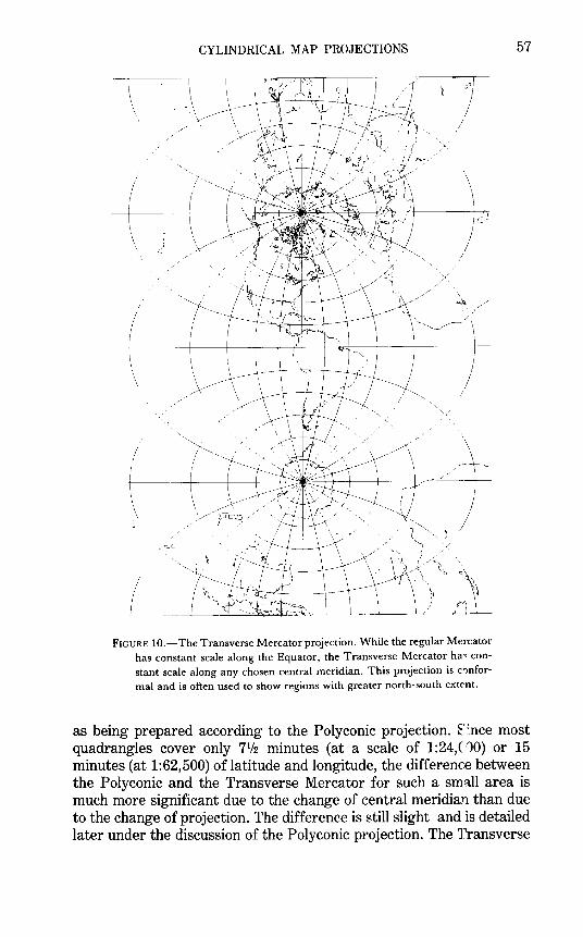
CYLINDRICAL MAP PROJECTIONS
\
I M. //
I - _.1
\ ~)-
FIGURE 10.-The Transverse Mercator projection. While the regular Mercator has constant scale along the Equator, the Transverse Mercator ha~ constant scale along any chosen central meridian. This projection is nnformal and is often used to show regions with greater north-south extent.
57
as being prepared according to the Polyconic projection. F:nce most quadrangles cover only 7112 minutes (at a scale of 1:24,('00) or 15 minutes (at 1:62,500) of latitude and longitude, the difference between the Polyconic and the Transverse Mercator for such a sm!ill area is much more significant due to the change of central meridian than due to the change of projection. The difference is still slight and is detailed later under the discussion of the Polyconic projection. The Transverse
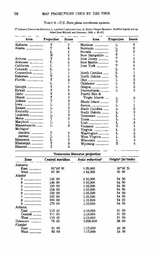
58 MAP PROJECTIONS USED BY THE USGS
TABLE 8. - U.S. State plane coordinate systems
[T indicates Transverse Mercator; L, Lambert Conformal Conic; H, Hotine Oblique Mercator. Modified slightly and up· dated from Mitchell and Simmons, 1945, p. 45-47]
Area Projection Zones Area Projection Zones
Alabama -------- T 2 Montana -------- L 3 Alaska ---------- T 8 Nebraska -------- L 2
L 1 Nevada --------- T 3 H 1 New Hampshire __ T 1
Arizona --------- T 3 New Jersey ------ T 1 Arkansas -------- L 2 New Mexico ______ T 3 California ------- L 7 New York------- T 3 Colorado -------- L 3 L 1 Connecticut ------ L 1 North Carolina ___ L 1 Delaware-------- T 1 North Dakota ____ L 2 Florida ---------- T 2 Ohio ------------ L 2
L 1 Oklahoma ------- L 2 Georgia --------- T 2 Oregon ---------- L 2 Hawaii ---------- T 5 Pennsylvania _____ L 2 Idaho ----------- T 3 Puerto Rico & Illinois ---------- T 2 Virgin Islands __ L 2 Indiana --------- T 2 Rhode Island _____ T 1 Iowa ------------ L 2 Samoa ---------- L 1 Kansas ---------- L 2 South Carolina ___ L 2 Kentucky -------- L 2 South Dakota ____ L 2 Louisiana -------- L 3 Tennessee ------- L 1 Maine ----------- T 2 Texas ----------- L 5 Maryland -------- L 1 Utah ------------ L 3 Massachusetts ____ L 2 Vermont T 1 Michigan1 --------
Virginia --------- L 2 obsolete ------- T 3 Washington ______ L 2 current-------- L 3 West Virginia ____ L 2
Minnesota ------- L 3 Wisconsin ------- L 3 Mississippi ------- T 2 Wyoming-------- T 4 Missouri --------- T 3
Transverse Mercator projection
Zone Central meridian Scale reduction2 Origins (la~itude)
Alabama East ------- 85°50' w. 1:25,000 30°30'' N. West ------- 87 30 1:15,000 30 00
Alaska4
2 ---------- 142 00 1:10,000 54 00
3 ---------- 146 00 1:10,000 54 00
4 ---------- 150 00 1:10,000 54 00
5 ---------- 154 00 1:10,000 54 00
6 ---------- 158 00 1:10,000 54 00
7 ---------- 162 00 1:10,000 54 00
8 ---------- 166 00 1:10,000 54 00
9 ---------- 170 00 1:10,000 54 00 Arizona
East _______ 110 10 1:10,000 31 00 Central _____ 111 55 1:10,000 31 00 West ------- 113 45 1:15,000 31 00
Delaware ------ 75 25 1:200,000 38 00 Florida4
East ------- 81 00 1:17,000 24 20 West ------- 82 00 1:17,000 24 20
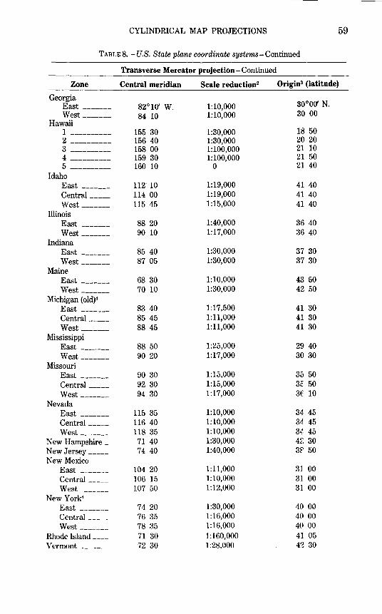
CYLINDRICAL MAP PROJECTIONS 59
TABLES. -U.S. State plane coordinate systems-Continued
Transverse Mercator projection- Continued
Zone Central meridian Scale reduction2 Origins (latitnde)
Georgia 30°00' N. East ------- 82°10' w. 1:10,000
West _______ 84 10 1:10,000 30 00 Hawaii
1 ---------- 155 30 1:30,000 18 50
2 ---------- 156 40 1:30,000 20 20
3 ---------- 158 00 1:100,000 21 10
4 ---------- 159 30 1:100,000 21 50
5 ---------- 160 10 0 21 40 Idaho
East _______ 112' 10 1:19,000 41 40' Central _____ 114 00 1:19,000 41 40
West ------- 115 45 1:15,000 41 40 Illinois
East _______ 88 20 1:40,000 36 40 West _______ 90 10 1:17,000 36 40
Indiana East ------- 85 40 1:30,000 37 30
West------- 87 05 1:30,000 37 30 Maine
East ------- 68 30 1:10,000 43 50
West ------- 70 10 1:30,000 42 50 Michigan ( old)4
East _______ 83 40 1:17,500 41 30 Central _____ 85 45 1:11,000 41 30
West ------- 88 45 1:11,000 41 30 Mississippi
East _______ 88 50 1:25,000 29 40 West _______ 90 20 1:17,000 30 30
Missouri East _______ 90 30 1:15,000 35 50 Central _____ 92 30 1:15,000 35 50 West _______ 94 30 1:17,000 3E 10
Nevada East _______ 115 35 1:10,000 34 45 Central _____ 116 40 1:10,000 34 45 West _______ 118 35 1:10,000 34 45
New Hampshire _ 71 40 1:30,000 4~ 30 New Jersey _____ 74 40 1:40,000 3f 50 New Mexico
East _______ 104 20 1:11,000 31 00 Central _____ 106 15 1:10,000 31 00 West _______ 107 50 1:12,000 31 00
New York4
East _______ 74 20 1:30,000 40 00 Central _____ 76 35 1:16,000 40 00 West _______ 78 35 1:16,000 40 00
Rhode Island ____ 71 30 1:160,000 41 05 Vermont _______ 72 30 1:28,000 42 30
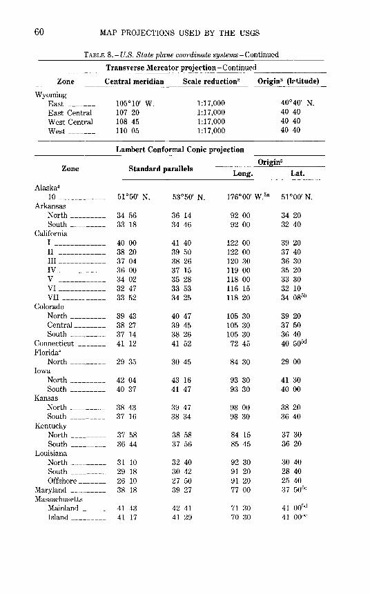
60 MAP PROJECTIONS USED BY THE USGS
TABLE 8.-U.S. Sta.te plane coordinate systems-Continued
Zone
Wyoming East ______ _
East Central West Central West ______ _
Transverse Mercator projection- Continued
Central meridian
105°10' w. 107 20 108 45 110 05
Scale reduction2
1:17,000 1:17,000 1:17,000 1:17,000
Lambert Conformal Conic projection
Origin3 (lrtitude)
40°40' N. 40 40 40 40 40 40
Origin5
Zone Standard parallels Long. Lat.
Alaska4
10 -----------Arkansas
North ________ _ South ________ _
California
I -------------II ___________ _ III ___________ _ IV ___________ _
v ------------VI ___________ _ VII __________ _
Colorado North ________ _ Central _______ _ South ________ _
Connecticut ______ _ Florida4
North ________ _ Iowa
North ________ _ South ________ _
Kansas North ________ _ South ________ _
Kentucky North ________ _ South ________ _
Louisiana North ________ _ South ________ _ Offshore ______ _
Maryland ________ _ Massachusetts
Mainland _____ _ Island ________ _
51°50' N.
34 56 33 18
40 00 38 20 37 04 36 00 34 02 32 47 33 52
39 43 38 27 37 14 41 12
29 35
42 04 40 37
38 43 37 16
37 58 36 44
31 10 29 18 26 10 38 18
41 43 41 17
36 14 34 46
41 40 39 50 38 26 37 15 35 28 33 53 34 25
40 47 39 45 38 26 41 52
30 45
43 16 41 47
39 47 38 34
38 58 37 56
32 40 30 42 27 50 39 27
42 41 41 29
92 00 92 00
122 00 122 00 120 30 119 00 118 00 116 15 118 20
105 30 105 30 105 30
72 45
84 30
93 30 93 30
98 00 98 30
84 15 85 45
92 30 91 20 91 20 77 00
71 30 70 30
51 °00' N.
34 20 32 40
39 20 37 40 36 30 35 20 33 30 32 10 34 085b
39 20 37 50 36 40 40 505d
29 00
41 30 40 00
38 20 36 40
37 30 36 20
30 40 28 40 25 40 37 5or•c
41 oor·d 41 oo'·c
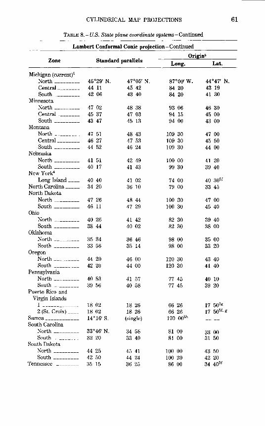
CYLINDRICAL MAP PROJECTIONS 61
TABLE 8.- U.S. State plane coordinate systems- Continued
Lambert Conformal Conic projection- Continued
Zone Standard parallels Origin6
Long. Lat.
Michigan (current)4
North--------- 45°29' N. 47°05' N. 87°00' w. 44°47' N. Central ________ 44 11 45 42 84 20 43 19 South _________ 42 06 43 40 84 20 41 30
Minnesota North _________ 47 02 48 38 93 06 46 30 Central ________ 45 37 47 03 94 15 45 00 South _________ 43 47 45 13 94 00 43 00
Montana North _________ 47 51 48 43 109 30 47 00 Central ________ 46 27 47 53 109 30 45 50 South _________ 44 52 46 24 109 30 44 00
Nebraska North _________ 41 51 42 49 100 00 41 20 South _________ 40 17 41 43 99 30 39 40
New York4
Long Island ____ 40 40 41 02 74 00 40 305f North Carolina _____ 34 20 36 10 79 00 33 45 North Dakota
North _________ 47 26 48 44 100 30 47 00 South _________ 46 11 47 29 100 30 45 40
Ohio North _________ 40 26 41 42 82 30 39 40 South _________ 38 44 40 02 82 30 38 00
Oklahoma North _________ 35 34 36 46 98 00 35 00 South _________ 33 56 35 14 98 00 33 20
Oregon North _________ 44 20 46 00 120 30 43 40 South _________ 42 20 44 00 120 30 41 40
Pennsylvania North _________ 40 53 41 57 77 45 40 10 South _________ 39 56 40 58 77 45 39 20
Puerto Rico and Virgin Islands
1 ------------- 18 02 18 26 66 26 17 505g
2 (St. Croix) ____ 18 02 18 26 66 26 17 505f· g
Samoa------------ 14°16' S. (single) 110 oo5h
South Carolina North _________ 33°46' N. 34 58 81 00 33 00 South _________ 32 20 33 40 81 00 31 50
South Dakota North _________ 44 25 45 41 100 00 43 50 South _________ 42 50 44 24 100 20 42 20
Tennessee ________ 35 15 36 25 86 00 34 40;,r
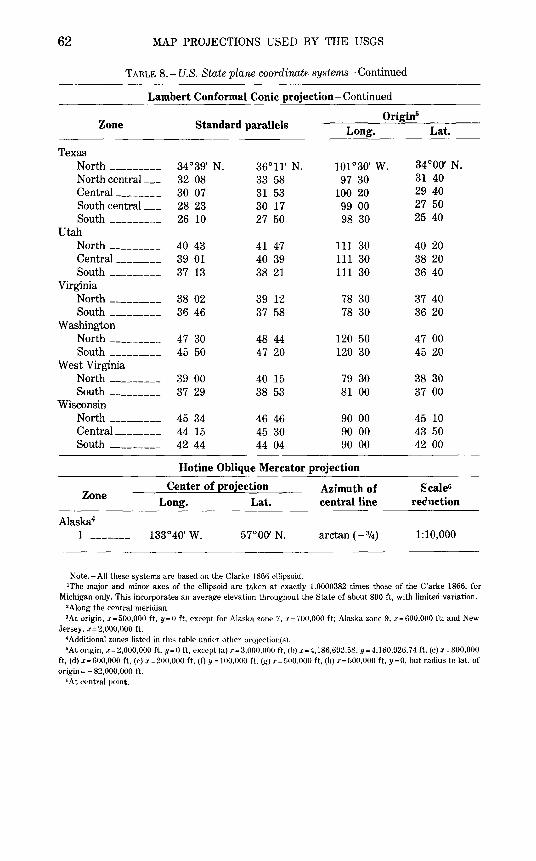
62 MAP PROJECTIONS USED BY THE USGS
TABLE 8.- U.S. State plane coordinate systems- Continued
Lambert Conformal Conic projection- Continued
Zone Standard parallels Origin5
Long. Lat.
Texas North --------- 34°39' N. 36°11' N. 101 °30' w. 34°00' N. North central ___ 32 08 33 58 97 30 31 40 Central ________ 30 07 31 53 100 20 29 40 South central ___ 28 23 30 17 99 00 27 50 South --------- 26 10 27 50 98 30 25 40
Utah North --------- 40 43 41 47 111 30 40 20 Central ________ 39 01 40 39 111 30 38 20 South--------- 37 13 38 21 111 30 36 40
Virginia North --------- 38 02 39 12 78 30 37 40 South --------- 36 46 37 58 78 30 36 20
Washington North _________ 47 30 48 44 120 50 47 00 South --------- 45 50 47 20 120 30 45 20
West Virginia North _________ 39 00 40 15 79 30 38 30 South --------- 37 29 38 53 81 00 37 00
Wisconsin North--------- 45 34 46 46 90 00 45 10 Central -------- 44 15 45 30 90 00 43 50 South _________ 42 44 44 04 90 00 42 00
Hotine Oblique Mercator projection
Zone Center of erojection Azimuth of Scale6
Long. Lat. central line re(htction
Alaska4
1 ------- 133°40' w. 57°00' N. arctan ( - 3f4) 1:10,000
Note.- All these systems are based on the Clarke 1866 ellipsoid. 'The major and minor axes of the ellipsoid are taken at exactly 1.0000382 times those of the C'arke 1866, for
Michigan only. This incorporates an average elevation throughout the State of about 800ft, with limited variation. 2Aiong the central meridian. 3At origin, .r=500,000 ft, y=O ft, except for Alaska zone 7, .r=700,000 ft; Alaska zone 9, .r=600,000 ft; and New
Jersey, :r=2,000,000 ft. 4Additional zones listed in this table under other projection(s). 5At origin, .r= 2,000,000 ft, y= 0 ft, except (a) .t=3,000,000 ft, (b) .r=4, 186,692.58, y=4,l60,926. 74ft. (c) .r=800,000
ft, (d) x=600,000 ft, (e) .r =200,000 ft. (f) 11= 100,000 ft, (g) .r= 500,000 ft, (h) .r=500,000 ft, y=O, but radius to lat. of origin= - 82,000,000 ft.
"At central point.
CYLINDRICAL MAP PROJECTIONS 63
Mercator is used in many other countries for official topographic mapping as well. The Ordnance Survey of Great Britain began switching from a Transverse Equidistant Cylindrical (the Cassini-Soldner) to the Transverse Mercator about 1920.
The use of the Transverse Mercator for quadrangle maps has been recently extended by the USGS to include the planets Me:"'cury and Mars. Although other projections are used at smallE:r scales, quadrangles at scales of 1:1,000,000 and 1:250,000, and covering areas from 200 to 800 km on a side, are drawn to the ellipsoidal T.-~ansverse Mercator between lats. 65° N. and S. on Mars, and to the spherical Transverse Mercator for any latitudes on Mercury. The sc-<:~Je factor along the central meridian is made 1. 0 in all cases.
In addition to its own series of larger-scale quadrangle maps, the Army Map Service used the Transverse Mercator for two other major mapping operations: (1) a series of 1:250,000-scale quadrangle maps covering the entire country, and (2) as the geometric bas-:q for the Universal Transverse Mercator (UTM) grid.
The entire area of the United States has been mapped since the 1940's in sections 2° of longitude (between even-numbered neridians, but in 3° sections in Alaska) by 1 o of latitude (between each full degree) at a scale of 1:250,000, with the UTM grid superimposed and with some variations in map boundaries at coastlines. These maps WE.re drawn with reference to their own central meridians, not the cent':'al meridians of the UTM zones (see below), although the 0.9996 certral scale factor was employed. The central meridian of about one-third of the maps coincides with the central meridian of the zone, but it does not for about two-thirds, the "wing" sheets, which therefore do not perfectly match the center sheets. The USGS has assumed publicatior and revision of this series and is casting new maps using the corre~t central meridians.
Transverse Mercator quadrangle maps fit continuously ir a northsouth direction, provided they are prepared at the same scale, with the same central meridian, and for the same ellipsoid. They do not fit exactly from east to west, if they have their own central neridians; although quadrangles and other maps properly constructed at the same scale, using the SPCS or UTM projection, fit in all directions within the same zone.
UNfVERSAL TRANSVERSE MERCATOR PROJECTION
The Universal Transverse Mercator (UTM) projection and grid were adopted by the U.S. Army in 1947 for designating rectangular coordinates on large-scale military maps of the entire world. Th~ UTM is the ellipsoidal Transverse Mercator to which specific parame~ers, such as central meridians, have been applied. The Earth, betweer lats. 84 °
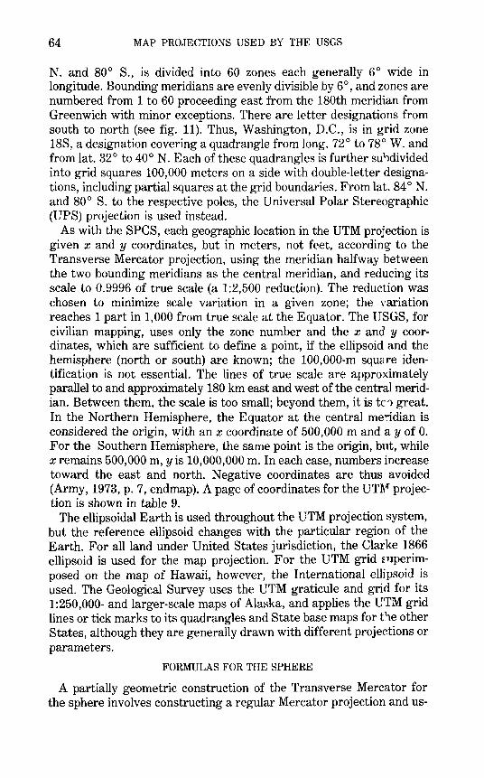
64 MAP PROJECTIONS USED BY THE USGS
N. and goo S., is divided into 60 zones each generally 6° wide in longitude. Bounding meridians are evenly divisible by 6 o, and zones are numbered from 1 to 60 proceeding east from the 1g0th meridian from Greenwich with minor exceptions. There are letter designations from south to north (see fig. 11). Thus, Washington, D.C., is in grid zone 1gs, a designation covering a quadrangle from long. 72° to 7go W. and from lat. 32° to 40° N. Each of these quadrangles is further su~divided into grid squares 100,000 meters on a side with double-letter designations, including partial squares at the grid boundaries. From lat. g4 ° N. and goo S. to the respective poles, the Universal Polar Stereographic (UPS) projection is used instead.
As with the SPCS, each geographic location in the UTM projection is given x and y coordinates, but in meters, not feet, according to the Transverse Mercator projection, using the meridian halfway between the two bounding meridians as the central meridian, and reducing its scale to 0.9996 of true scale (a 1:2,500 reduction). The reduction was chosen to minimize scale variation in a given zone; the variation reaches 1 part in 1,000 from true scale at the Equator. The USGS, for civilian mapping, uses only the zone number and the x and y coordinates, which are sufficient to define a point, if the ellipsoid and the hemisphere (north or south) are known; the 100,000-m square identification is not essential. The lines of true scale are approximately parallel to and approximately 180 km east and west of the central meridian. Between them, the scale is too small; beyond them, it is tC'0 great. In the Northern Hemisphere, the Equator at the central me':idian is considered the origin, with an x coordinate of 500,000 m and a y of 0. For the Southern Hemisphere, the same point is the origin, but, while x remains 500,000 m, y is 10,000,000 m. In each case, numbers increase toward the east and north. Negative coordinates are thus avoided (Army, 1973, p. 7, endmap). A page of coordinates for the UTI\"" projection is shown in table 9.
The ellipsoidal Earth is used throughout the UTM projection system, but the reference ellipsoid changes with the particular region of the Earth. For all land under United States jurisdiction, the Clarke 1g66 ellipsoid is used for the map projection. For the UTM grid E·uperimposed on the map of Hawaii, however, the International ellipsoid is used. The Geological Survey uses the· UTM graticule and grid for its 1:250,000- and larger-scale maps of Alaska, and applies the UTM grid lines or tick marks to its quadrangles and State base maps for tt:le other States, although they are generally drawn with different projections or parameters.
FORMULAS FOR THE SPHERE
A partially geometric construction of the Transverse Mercator for the sphere involves constructing a regular Mercator projection and us-
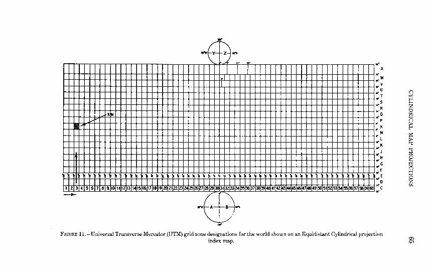
.. -tvt:J~ .. ... ...
I I I X rt' ,.
I w
1/('
v .. u
_.T .. 5
!¥' R
3N ... Q
............ ... p
II""" ..
N .. f-~
M .. L ...
K tl('
J r
H .. .. G
~ ~ '! ~~l!~l!~~'!~'!'!1tlt!al!1:k ~\\1t1t111!!!lolo .. ~~\\1t. 1: l! lt1t~'!~'!~~l!~l!l!1!'!~'!
I I 1 21 314 5 6 7 8 9. 10 1112 13 14j15 16 17 18 19 20 21 22 23 24 25 26 27 28 29l3q31 32 33 34j35j36137 38 39 40 41 42!4Jj44 45 46 47j4al49 50 51 52 53 54 55 56 57 58 59 601
_.F E
1/('
D ,,. c ..
... FIGURE 11.- Universal Transverse Mercator (UTM) grid zone designations for the world shown on an Equidistant Cylindrical projection
index map.
(1
~ l' z t;j ~ ......... (1
> l'
s= > '"0
'"0
~ I:..;
M (1 t-3 0 z r.n
Q':) 01
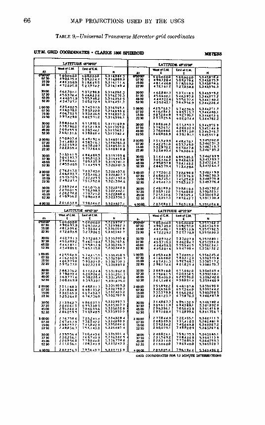
66 MAP PROJECTIONS USED BY THE USGS
TABLE 9.- Universal Transverse Mercator grid coordinates
U.T.M. GRID COORDINATES • CLARKE 1866 SPHEROID Mll'ERS
LATITUDE 48"00'00" LATITUDEW15'00" WesloiC.M. EastoiC.M. WestoiC.M. EastoiC.M. 1\). E E N &~ E E N v;; 5 oo.ooo.o 5 oo.ooo.o 5,316.~81.~
~ 5oo.ooo.o 5 oo.ooo.o 5,3A3.8~8.4 .. 90,6 7'5.3 5 09,32A.7 5.316,088.9 A90,720.A 509.279.6 5,3A3,875.9 1500 A 81,350.5 5 18.649.'5 5,316,111.6 1500 A81,440.8 5 I 8.5 59.2 5,343.8~8.6 2230 1172.025.8 52 7.9 74.2 5,316.1A9 4 2230 A 72.161.2 52 7.838.8 5,3A3,916.3
3000 .. 62,701.1 5 37.2 98.9 5.316.202.3 3000 .. 62,881.7 5 37.1183 5.3A3,919.Z 3730 A53.376.A 5 46,6 23.6 5,316.270.3 3730 4 53.602.1 5 46.3 97.9 5,3AA,0,7 .2 4500 .. 4 4.051.8 555,948.2 5,316.353.5 4500 • 4 ... 322.6 5 55,6 77.4 5,34A,IA0.2 5230 1134.727.1 5 65.272.9 5.316.A51.7 5230 435.043.1 56A.956.9 5.34A.238.4
10000 4 25.A02.5 5 74.597.5 5.316.565.1 10000 A 25.763.7 57 A.2 36.3 5,344,3"11.7 0730 .. 16.078.0 5 83,922.0 5.316.693.6 0730 4 16.4 84.3 583,515.7 5.3AA.480.1 1500 4 06.753.5 5 93.2 46.5 5.316.837 3 1500 4 07.204.9 5 92,7 95.1 5.3 44,6~ 3.6 2230 397,429.0 602.5 71.0 5.316.996.1 2230 3 97.92'5.6 6 02.074.4 5.3 4 4.7 82 .2
3000 388.104.5 611,8955 5.317,169.9 3000 3 88.646.3 6 11,353.7 5.3 44,9"i5 9 3730 3 78.780.2 6 21,219.8 5.317.359.0 3730 379.367.1 6 20.6 32.9 5,345.144 8 4500 3 69,455.9 630,544.1 5,317.563.1 4500 3 70,088.0 6 29.91 2·0 5,3 45.3 ~ 8.7 5230 3 60.131.6 6 3 9,8 68.4 5,317.782.4 5230 360,808.9 6 39.191.1 5.345.5'\ 7 8
20000 3 50,807.4 6 49.192.6 5,318.016 8 20000 351,529.9 6 4 8.4 70.1 '>.345.r02.0 0730 3 41,4 83.3 6 58.516.7 5.318.266.3 0730 3 42.25 t.O 657,7419.0 5,346.C'51.3 1500 332.159.3 6 6 7.8 40.7 5.31 8.5 31 .0 1500 332,972.2 6 67.027.8 5,3 46,, 5.7 2230 3 2 2.8 35.4 6 77.164.6 5,318.8108 2230 3 2 3,693.4 6 76,306.6 5,346595.3
3000 3 13.511 5 6 86.488.5 5,319.105 8 3000 :514.414.8 6 85,585.2 5,3 46,e'89.9 3730 30A.187.7 6 95,812.3 5,319.AI5.9 3730 3 05.136.2 694,863.8 5,347.199.7 4500 2 94.864.1 705.135.9 5.319.7 41 .I 4500 2 95.857.8 7 04.1 42.2 5,347,5'24.7 5230 2 85.540.5 7 IA.459.5 5,320,081.5 !1230 2 86.5 79.4 7 13,420.6 5,3A7.e'64.7
30000 Z 76.2 I 7.0 7 23.783.0 5.320,437.0 30000 277,301.2 7 22,6 98.8 5,3 48,Z I 9.9 0730 z 66.893.7 7 33.106.3 5,3 20.80 7.7 0730 2 68.023.1 73t,976.9 5,348,590.3 1500 z 5 7,5 70.5 7 42,1129 5 5,321,1 9J .6 1500 Z 58,7 A5.1 7 41,254.9 5,3 485'75 .8 2230 z 118.2414 7 51,7 52.6 5,321,594.6 2230 2 49.467.3 7 50,532.7 5,3 A9,!176.4
3000 2 38.924 4 761,075.6 5.322,010.8 3000 2 A0,189.6 7 5 9,810.4 5,3A9.792.Z 3730 2 2 9.60 I 5 7 70,398.5 5.32Z,A42.1 3730 2 30,912.0 7 6 9,088.0 5,350.<'23.1 4500 2 20.2 78.8 7 79.721.2 5,3 22,888.6 4500 2 21,6 34.6 7 7 8.3 65.4 5,3 50,669.2 5230 210,9562 7 89.043.8 5.323.350 3 52 30 212.357.3 7 8 7.6 42 7 5,351,130.4
40000 2 01,6 33.8 7 98.366.2 5,323.82 7 .I 400.00 2 03.080 2 7 96.91 9.8 5.3 51 E06 8
LATITUDE 48"0?'30" LATITUDE -68"'22'30" WestofC.M. EntoiC.M. WestoiC.M. EaslofC.M.
1\). E E N A •. E E N
v;:- ~ C!II·Ooo.o 5 oo.ooo.o ~:H:·:~; ~ ~~ 5 C!~·ooo.o 5 Olj.ooo.o ~:~~;:~:;; 4 90,6 97.8 50 9.302.2 4 90,7 413.0 5 09.257.0 1500 4 81,395.6 5 I 8.6 04 4 5.3 30.004 9 1500 4 81,486.1 518.513.9 5.357,192.5 2230 4 72.093.5 527.9065 ';.330,042 7 2230 4 72.229.2 5 27,7 70.8 5.357.830.3
3000 1162,7913 5:57.208.7 5.3 30.095.6 3000 4 62.972.2 53 7.027.8 5,357.883 1 3730 4 5 3,4 892 54 6.5 I 0.8 5,330,163.6 3730 453.715.3 5 416.2841 7 5.35U51.0 4500 4 4 4,1 87.1 5 55.812.9 5.3 30,2416.7 4500 4 44.4158.5 5 55.5 41 5 S.358C'34.1 5230 4 34885 0 5 65.1 15.0 5.3 30.344.9 5230 .. 35.201 6 564,7984 5.3 58.132 2
10000 4 2 5.5 82.9 57 4.417.1 5.3 30.458 3 10000 41 2'5.944.8 5741,0552 5.3 58.2 415.4 0730 416.2809 583,719.1 5,3 30.586 7 0730 4 I 6.6 88.0 58 3.312 0 5.358.373 8 1500 4 06.979.0 5 93,021.0 5,3 30.730 3 1500 4 07.4 31.3 5 92,568.7 5.358.! I 7.2 2230 3 97.6 77.0 6 02.323.0 5,3 30.88 9.0 2230 3 98.1 74.6 601,8254 5.3 58.f 75.7
3000 3 88.375.2 6 I 1,624.8 5.331,062 8 3000 3 88,918.0 6 1 1,082.0 5,358F49 4 3730 ~ 7 9,0 73 4 620.926.6 5.331,251.7 3730 3 7 9.6" .5 6 2 0.~~8 5 5.:559.('~8.1 4500 369.7716 630.228.4 '5.3 31.455 8 4500 3 70,4 05.0 6.2 9,5 95.0 5.:559.4!42 0 5230 360,469.9 6 39.530.1 '>.-' 31,6 75.0 5230 361.148.6 6 38.8 51 4 5.359460 9
2 0000 351,1683 648.8317 5,331,909.3 20000 3 51,8 92.2 6 48.107.8 5,3 59.E 95.0 0730 3 41,866.8 6 58.133.2 5,332,158.7 0730 3 42.636.0 657.364.0 5,359.N4.Z 1500 3 32.565 3 6 67.434.7 5,332.423.2 1500 3 33.3 79.a 6 66,620.2 '5,360.<'08 5 2230 3 23.264.0 6 76.7 36.0 5. 3 32,70 2 .9 2230 324.123.7 6 75.876.3 5.:560.-'a7.9
3000 3 13.962.7 6 86.037 3 5.332.997.7 3000 314.867.7 6a5.1323 5.3 60.782 • 3730 3 04.661 5 6 95.33a 5 5,333,307.7 3730 3 05.61 1.9 6 94,3a8.1 5.361,092.0 4500 2 95.3 60.4 7 OA,6 39.6 '5.333,632 8 4500 2 96.356.1 7 03.6113.9 5.361,416 a 5230 2 86.059.5 7 I 3,9 40.5 5.3 33.973.0 5230 287.100.4 7 12,899.6 5.361.7567
30000 z 76.758 6 7 2 3,2 41.4 5.3 34,328 4 30000 2 77,844.9 7 22.155.1 '5.362,111 7 0130 2 6 7.4 57.9 732.5422 5.334.698 9 0730 2 68.589.5 7 31,410.5 5.!162.481 9 1500 258.1572 741,8428 5.335.084 6 1500 z 59.334.2 7 40,665.8 '5,3 62.!'6 7.2 2230 z 4a.856.7 751,143.3 5.3 35.4 8'5 4 2230 2 50,079.1 149.920.9 5.3 63,<'6 7 6
3000 2 39.556 4 7 60,4 43 6 5.:5 35.90 I 4 3000 z 40,824.1 759.175.9 5.36:5,(8:5.1 37 30 2 30.256.1 769.7439 5.3 36.332 5 3730 2 31,569.2 768.430 a '5,364.113 9 4500 2 20.9 56.0 7 79.044.0 5.~36.778 8 4500 2 22.314.5 7 77.6 85.5 5.364.!'59.7 5230 Z I 1,656.1 7 8 8.3 4 3 9 5,337.240 3 52 30 2 I 3.060.0 7 8 6.9 4 o.o '5,365.CI20 7
40000 z 02.356 3 7 97.6 43 7 5.337.716 9 40000 2 03.8056 796.194.4 5365-'968
GRID COORDINATES FOR 7.5 MINYI'£ INTERSECTIONS
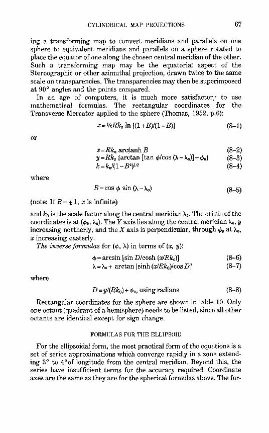
CYLINDRICAL MAP PROJECTIONS 67
ing a transforming map to convert meridians and paralle]s on one sphere to equivalent meridians and parallels on a sphere r1tated to place the equator of one along the chosen central meridian of the other. Such a transforming map may be the equatorial aspect of the Stereographic or other azimuthal projection, drawn twice to the same scale on transparencies. The transparencies may then be superimposed at 90° angles and the points compared.
In an age of computers, it is much more satisfactor:r to use mathematical formulas. The rectangular coordinates for the Transverse Mercator applied to the sphere (Thomas, 1952, p.6):
X= 112Rk0 In [(1 +B)/(1-B)] (8-1)
or
x=Rko arctanh B (8-2) y=Rk0 {arctan [tan ¢/cos (A-Ao)]-c/>o} (8-3) k = ko/(1-B 2
)112 (8-4)
where
B=cos cJ> sin (A-Ao)
(note: If B= ± 1, xis infinite)
(8-5)
and k0 is the scale factor along the central meridian Ao. The orisin of the coordinates is at (c/>o, A0). The Yaxis lies along the central meridian Ao, y increasing northerly, and the X axis is perpendicular, through c/>o at Ao, x increasing easterly.
The inverse formulas for (c/>, A) in terms of (x, y):
cp=arcsin [sinD/cosh (x/Rk0)]
A= Ao + arctan [sinh (x/Rk0)/cos D]
where
D = yi(Rk0 ) + c/>o, using radians
(8-6) (8-7)
(8-8)
Rectangular coordinates for the sphere are shown in table 10. Only one octant (quadrant of a hemisphere) needs to be listed, since all other octants are identical except for sign change.
FORMULAS FOR THE ELLIPSOID
For the ellipsoidal form, the most practical form of the equr.tions is a set of series approximations which converge rapidly in a zon~ extending 3° to 4°of longitude from the central meridian. Beyond this, the series have insufficient terms for the accuracy required. Coordinate axes are the same as they are for the spherical formulas above. The for-
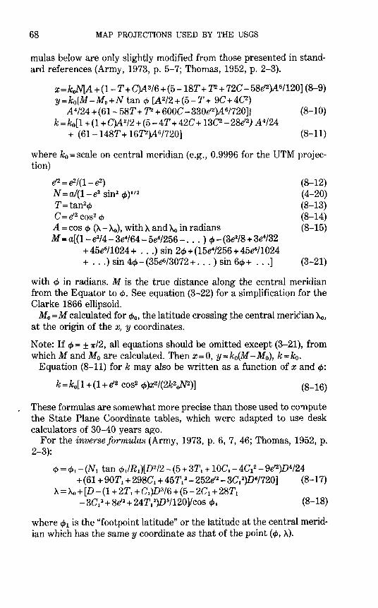
68 MAP PROJECTIONS USED BY THE USGS
mu1as below are only slightly modified from those presented in standard references (Army, 1973, p. 5-7; Thomas, 1952, p. 2-3).
X= koN[A + (1- T + C)A 3/6 + (5- 18T + p. + 72C- 58e'2)A 5/120] (8-9) y=k0(M -Mo+N tan¢ [A2/2+(5- T+ 9C+4C2)
A 4/24 + (61- 58T + P. + 600C- 330e'2)A 6/720]} (8-10) k = k0[1 + (1 + C)A 2/2 + (5- 4T + 42C + 130- 28e'2) A 4/24
+ (61-148T+16P.)A6/720] (8-11)
where k0 =scale on central meridian (e.g., 0.9996 for the UTM projection)
e'2 = e2/(1- e2) N = a/(1- e2 sin2 ct> )112
T=tan2¢ C=e'2 cos2 ¢ A =cos ¢ (A- Ao), with A and Ao in radians M = a[(1- e2/4- 3e4/64- 5e6/256- ... ) cp- (3e2/8 + 3e4/32
+45e6/1024+ ... ) sin 2ct>+(15e4/256+45e6/1024 + ... ) sin 4cp- (35&/3072 + ... ) sin 6ct> + ... ]
(8-12) (4-20) (8-13) (8-14) (8-15)
(3-21)
with ¢ in radians. M is the true distance along the central meridian from the Equator to ¢. See equation (3-22) for a simplification for the Clarke 1866 ellipsoid.
M0 =M calculated for cl>o, the latitude crossing the central meridian Ao, at the origin of the x, y coordinates.
Note: If ct>= ± 7f'l2, all equations should be omitted except (3-21), from which M and M0 are calculated. Then x=O, y=k0(M -M0), k=k0 •
Equation (8-11) fork may also be written as a function of x and cp:
(8-16)
, These formulas are somewhat more precise than those used to co~pute the State Plane Coordinate tables, which were adapted to use desk calculators of 30-40 years ago.
For the inverse formulas (Army, 1973, p. 6, 7, 46; Thomas, 1952, p. 2-3):
¢=c/>.-(N1 tan cJ>./R1)[D2/2-(5+3T. + 10C.-4C12-9e'2)D4/24
+(61 +90Tt +298Ct +45T12 -252e'2 -3C1
2)D6/720] (8-17) A=Ao+[D -(1 +2T. +C.)D3/6+(5-2Cl +28Tl
-3C12 +8e'2 +24Tl)D5/120]/cos cl>t (8-18)
where cp1 is the "footpoint latitude" or the latitude at the central meridian which has the same y coordinate as that of the point (ct>, >-.).
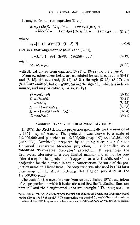
CYLINDRICAL MAP PROJECTIONS 69
It may be found from equation (3-26):
<1>1 = p. + (3e1/2- 27 e13/32 + ... ) sin 2p. + (21e12/16 -55e1432- ... ) sin 4p.+(151e1
3/96+ ... ) sin 6p.+ ... (3-26)
where el = [1- (1- e2)1'2]/[1 + (1- e2)1'2]
and, in a rearrangement of (3-20) and (3-21),
p. =MI[a(1- e2/4- 3e4/64- 5e6/256- ... )]
while
(3-24)
(8-19)
(8-20)
with Mo calculated from equation (3-21) or (3-22) for the given c/>o. From <1>1, other terms below are calculated for use in equations (8-17)
and (8-18). (If c/>1 = ± 1r/2, (8-12), (8-21) through (8-25), (8-17) and (8-18) are omitted, but <t> = ± 90°, taking the sign of y, while A is indeterminate, and may be called Ao. Also, k=ko.)
ff2 = e2/(1- e2) c1 =.e2COS2<I>t T1 =tan2¢, N1 = a/(1- e2sin2¢~)" 2
R, = a(1- e2)/(1- e2sin2<t>1)312
D=xi(N,ko)
"MODIFIED TRANSVERSE MERCATOR" PROJECTIO.IY
(8-12) (8-21) (8-22) (8-23) (8-24) (8-25)
In 1972, the USGS devised a projection specifically for the revision of a 1954 map of Alaska. The projection was drawn to a scale of 1:2,000,000 and published at 1:2,500,000 (map "E") and 1:1,584,000 (map "B"). Graphically prepared by adapting coordinates for the Universal Transverse Mercator projection, it is identified as a "Modified Transverse Mercator" projection. It resembles the Transverse Mercator in a very limited manner and cannot be considered a cylindrical projection. It approximates an Equidistant Conic projection for the ellipsoid in actual construction. Because of the projection name, it is listed here. The projection was also used h 1974 for a base map of the Aleutian-Bering Sea Region publisl,~d at the 1:2,500,000 scale.
The basis for the name is clear from an unpublished 1972 description of the projection, in which it is also stressed that the "latitudinal lines are parallel" and the "longitudinal lines are straight." The computations
"were taken from the AMS Technical Manual #21 (Universal Transverse Mercator) based on the Clarke 1866 Spheroid.*** The projection was started from a N-S ce'ltral construction line of the 153° longitude which is also the centerline of Zone 5 from tlr-> UTM tables.
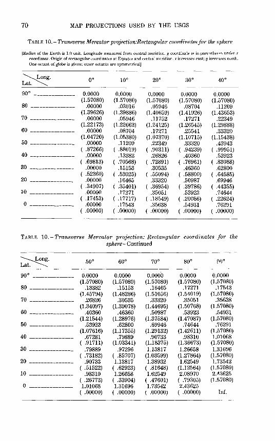
70 MAP PROJECTIONS USED BY THE USGS
TABLE 10.-Transverse Mercator p'rojection:RActangular coordinates for the sphere
[Radius of the Earth is I .0 unit. Longitude measured from central meridian. y coordinate is in parenthe>ces under x coordinate. Origin of rectangular coordinates at Equator and central meridian. x increases east; y incre'lses north. One octant of globe is given; other octants are symmetrical]
~· L oo 10° 20° 30° 40°
goo -------------- 0.0000 0.0000 0.0000 0.0000 0.0000 (1.57080) (1.57080) (1.57080) (1.57080) (1.57080)
80 --------------- .00000 .03016 .o5g46 .08704 .1120g (1.3g626) (1.3g886) (1.4065g) (1.41g26) (1.43653)
70 --------------- .00000 .o5g46 .11752 .17271 .2234g (1.22173) (1.22662) (1.24125) (1.26545) (1.2g888)
60 --------------- .00000 .08704 .17271 .25541 .33320 (1.04720) (1.05380) (1.07370) (1.10715) (1.15438)
50 --------------- .00000 .112og .2234g .33320 .43g43 ( .87266) ( .8801g) ( .go311) ( .g423g) ( .ggg51)
40 --------------- .00000 .13382 .26826 .40360 .53g23 ( .6g813) ( .70568) ( .728g1) ( .76g61) ( .83088)
30 --------------- .00000 .15153 .30535 .46360 .62800 ( .52360) ( .53025) ( .550g4) ( .58800) ( .64585)
20 --------------- .00000 .16465 .33320 .50g87 .6gg46 ( .34g07) ( .35401) ( .36g54) ( .3g786) ( .44355)
10 --------------- .00000 .17271 .35051 .53g23 .74644 ( .17453) ( .17717) ( .1854g) ( .20086) ( .22624)
0 --------------- .00000 .17543 .35638 .54g31 .762g1 ( .00000) ( .00000) ( .00000) ( .00000) ( .00000)
TABLE 10.- Transverse Mercator projection: Rectangular coordinates for the sphere- Continued
~· 50° 60° 70° 80° f'f)o .
goo -------------- 0.0000 0.0000 0.0000 0.0000 0.0000 (1.57080) (1.57080) (1.57080) (1.57080) (1.57080)
80 --------------- .13382 .15153 .16465 .17271 .17543 (1.457g4) (1.48286) (1.51056) (1.5401g) (1.57080)
70 --------------- .26826 .30535 .33320 .35051 .35638 (1.340g7) (1.3g078) (1.446g5) (1.50768) (1.57080)
60 --------------- .40360 .46360 .50g87 .53g23 .54g31 (1.21544) (1.28g76) (1.37584) (1.47087) (1.57080)
50 --------------- .53g23 .62800 .6gg46 .74644 .762g1 (1.07616) (1.17355) (1.2g132) (1.42611) (1.57080)
40 --------------- .67281 .7988g .go733 .98310 1.01068 ( .g1711) (1.03341) (1.18375) (1.36673) (1.57080)
30 --------------- .7g889 .97296 1.13817 1.26658 1.316g6 ( .73182) ( .85707) (1.035gg) (1.27864) (1.57080)
20 --------------- .go733 1.13817 1.38g32 1.6254g 1.73542 ( .51522) ( .62g23) ( .81648) (1.12564) (1.57080)
10 --------------- .g8310 1.26658 1.6254g 2.08g7o 2.A3625 ( .26773) ( .33g04) ( .47601) ( .7g305) (1.57080)
0 --------------- 1.01068 1.316g6 1.73542 2.43625 ( .00000) ( .00000) ( .00000) ( .00000) Inf.
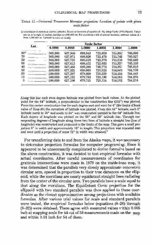
CYLINDRICAL MAP PROJECTIONS 71
TABLE 11.- Universal Transverse Mercator projection: Location of points with given scale factor
[ x coordinates in meters at various latitudes. Based on inversion of equation (8-16), using Clarke 1f~6 ellipsoid. Values are on or to right of central meridian (x= 500,000 m). For coordinates left of central meridian, subtract values of x from 1,000,000 m. Latitude is north or south]
Lat. Scale factor
0.9996 0.9998 1.0000 1.0002 1.000-1 1.0006
goo ----------- 500,000 627,946 6g0,943 721,609 755,g92 7g6,096 70 ----------- 500,000 627,g71 6go,g36 721,47g 755,741 7g5,927 60 ----------- 500,000 627,755 6g0,673 721,27g 755,510 7g5,66g 50 ----------- 500,000 627,613 6g0,472 721,032 755,22'1 7g5,352 40 ----------- 500,000 627,463 6g0,260 720,772 754,923 7g5,015 30 ----------- 500,000 627,322 6g0,060 720,52g 754,643 784,700 20 ----------- 500,000 627,207 679,g9g 720,329 754,414 784,443 10 ----------- 500,000 627,132 679,792 720,199 754,264 7g4,276 0 ----------- 500,000 627,106 679,755 720,154 754,212 7g4,21g
Along this line each even degree latitude was plotted from book values. At the plotted point for the 64 ° latitude, a perpendicular to the construction line (153°) was plotted. From the center construction line for each degree east and west for 4 o (the limits of book value of Zone #5) the curvature of latitude was plotted. From this 64 o latitude, each 2° latitude north to 70° and south to 54 o was constructed parallel to the 64 ° latitude line. Each degree of longitude was plotted on the 5go and 6go latitude line. Through corresponding degrees of longitude along these two lines of latitude a straight line (line of longitude) was constructed and projected to the limits of the map. This gave a small projection go in width and approximately 1go in length. This projection was repeated east and west until a projection of some 72° in width was attained."
For transferring data to and from the Alaska maps, it was necessary to determine projection formulas for computer programing. Since it appeared to be unnecessarily complicated to derive formul~.s based on the above construction, it was decided to test empirical formulas with actual coordinates. After careful measurements of coordinates for graticule intersections were made in 1979 on the stable-base map, it was determined that the parallels very closely approximate concentric circular arcs, spaced in proportion to their true distances on the ellipsoid, while the meridians are nearly equidistant straight lines radiating from the center of the circular arcs. Two parallels have a scale equal to that along the meridians. The Equidistant Conic projection for the ellipsoid with two standard parallels was then applied to these coordinates as the closest approximation among projections with available formulas. After various trial values for scale and standard parallels were tested, the empirical formulas below (equations (8-26) through (8-32)) were obtained. These agree with measured values vrithin 0.005 inch at mapping scale for 44 out of 58 measurements made on the map and within 0.01 inch for 54 of them.
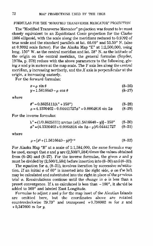
72 MAP PROJECTIONS USED BY THE USGS
FORMULAS FOR THE "MODIFIED TRANSVERSE MERCATOR" PROJECTION
The "Modified Transverse Mercator" projection was found to b8 most closely equivalent to an Equidistant Conic projection for the Clarke 1866 ellipsoid, with the scale along the meridians reduced to 0. 9J92 of true scale and the standard parallels at lat. 66.09° and 53.50° N. (also at 0.9992 scale factor). For the Alaska Map "E" at 1:2,500,000, using long. 150° W. as the central meridian and lat. 58° N. as the latitude of the origin on the central meridian, the general formulas (Snyder, 1978a, p. 378) reduce with the above parameters to the followin~, giving x and y in meters at the map scale. The Y axis lies along the central meridian, y increasing northerly, and the X axis is perpendicular at the origin, x increasing easterly.
For the forward formulas:
X= p sin 8 y = 1. 5616640- p cos ()
where
8° = 0.8625111(A 0 + 150°) p = 4.1320402- 0. 04441727 cp o + 0. 0064816 sin 2cp
For the inverse formulas:
where
A o =(110.8625111) arctan [x/(1.5616640-y)]-150° c/> 0 =(4.1320402+0.0064816 sin 2cp-p)/0.04441727
p = [x2 +(1.5616640- y)2)112
(8-26) (8-27)
(8-28) (8-29)
(8-30) (8-31)
(8-32)
For Alaska Map "B" at a scale of 1:1,584,000, the same formul2.s may be used, except that x andy are (2,500/1,584) times the values obtained from (8-26) and (8-27). For the inverse formulas, the given x and y must be divided by (2,500/1,584) before insertion into (8-30) and (8-32).
The equation for cp, (8-31), involves iteration by successive su':lstitution. If an initial cp of 60 o is inserted into the right side, cp on t'le feft may be calculated and substituted into the right in place of the pr~vious trial cp. Recalculations continue until the change in cp is less than a preset convergence. If A as calculated is less than -180°, it shcnld be added to 360° and labeled East Longitude.
Formulas to adjust x and y for the map inset of the Aleutian Islands are omitted here, but the coordinates above are rotated counterclockwise 29.79° and transposed +0.798982 m for x and +0,347600 m for y.
9. OBLIQUE MERCATOR PROJECTION
SUMMARY
• Cylindrical (oblique). • Conformal. • Two meridians 180° apart are straight lines. • Other meridians and parallels are complex curves. • Scale on the spherkal form is true along chosen central line, a great circle at an oblique
angle, or along two straight lines parallel to central line. The scale on the ellipsoidal form is similar, but varies slightly from this pattern.
• Scale becomes infinite 90° from the central line. • Used for grids on maps of the Alaska panhandle, for mapping in Switzerland,
Madagascar, and Borneo and for atlas maps of areas with greater extent in an oblique direction
• Developed 1900-50 by Rosenmund, Laborde, Hotine, and others.
HISTORY
There are several geographical regions such as the Alask8 panhandle centered along lines which are neither meridians nor parallels, but which may be taken as great circle routes passing through the region. If conformality is desired in such cases, the Oblique Mercator is a projection which should be considered.
The historical origin of the Oblique Mercator projection d':les not appear to be sharply defined, although it is a logical generalization of the regular and Transverse Mercator projections. Apparently, Posenmund (1903) made the earliest published reference, when he devis~d an ellipsoidal form which is used for topographic mapping of Switzerland. The projection was not mentioned in the detailed article on "Map Projections" in the 1911 Encyclopaedia Britannica (Close and Clarl·e, 1911) or in Hinks' brief text (1912). Laborde applied the Oblique Mercator to the ellipsoid for the topographic mapping of Madagascar in 1928 (Young, 1930; Laborde, 1928). H. J. Andrews (1935, 1938) proposed the spherical forms for maps of the United States and Eurasia. Hinks presented seven world maps on the Oblique Mercator, with poles located in several different positions, and a consequent variety in the regions shown more satisfactorily (Hinks, 1940, 1941).
A study of conformal projections of the ellipsoid by British geodesist Martin Hotine (1898-1968), published in 1946-47, is the b:tsis of the U.S. use of the ellipsoidal Oblique Mercator, which Hotine called the "rectified skew orthomorphic" (Hotine, 194 7, p. 66-67). The Hotine approach has limitations, as discussed below, but it provides closed formulas which have been adapted for U.S. mapping of suitable zones.
73
74 MAP PROJECTIONS USED BY THE USGS
One of its limitations is overcome by a recent series form of tl' ~ ellipsoidal Oblique Mercator (Snyder, 1979a, p. 74), but other limitations result instead. This later form resulted from development of f<'-..mulas for the continuous mapping of satellite images, using the Space Oblique Mercator projection (to be discussed later).
While Hotine projected the ellipsoid conformally onto an "aposphere" of constant total curvature and thence to a plane, Laborde and also J. H. Cole (1943, p. 16-30) projected the ellipsoid onto a "conformal sphere," using conformal latitudes (described earlier) to mr~e the spi1ere conformal with respect to the ellipsoid, then plotted the spherical Oblique Mercator from this intermediate sphere. Rosenround's system for Switzerland is a more complex double projection through a conformal sphere (Rosenmund, 1903; Bolliger, 1967:,
FEATURES
The Oblique Mercator for the sphere is equivalent to a regular Mercator projection which has been altered by wrapping a cylinder around the sphere so that it touches the surface along the great circ1~ path chosen for the central line, instead of along the Earth's Equator. A set of transformed meridians and parallels relative to the great circle may be plotted bearing the same relationship to the rectangular cooriinates for the Oblique Mercator projection, as the geographic meridir.ns and parallels bear to the regular Mercator. It is, therefore, possible to convert the geographic meridians and parallels to the transformed values and then to use the regular Mercator equations, substituting the transformed values in place of the geographic values. This is the procedure for the sphere, although combined formulas are given below, but it becomes much more complicated for the ellipsoid. The ad'Tent of present-day computers and programmable pocket calculatorr make these calculations feasible for sphere or ellipsoid.
The resulting Oblique Mercator map of the world (fig. 12) thus resembles the regular Mercator with the landmasses rotated so that the poles and Equator are no longer in their usual positions. Instead, two points 90° away from the chosen great circle path through the center of the map are at infinite distance off the map. Normally, the Oblique Mercator is used only to show the region near the central line and for a relatively short portion of the central line. Under these conditions, it looks similar to maps of the same area using other projE'I'~tions, except that careful scale measurements will show differences.
It should be remembered that the regular Mercator is in fact a limiting form of the Oblique Mercator with the Equator as the central line, while the Transverse Mercator is another limiting form of the Oblique with a meridian as the central line. As with these limiting
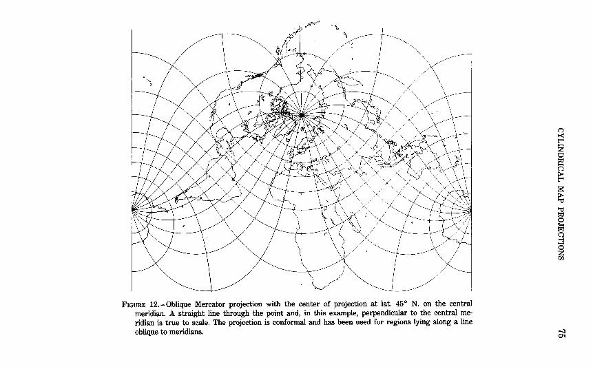
,trc:?
FIGURE 12.-Oblique Mercator projection with the center of projection at lat. 45 ° N. on the central meridian. A straight line through the point and, in this example, perpendicular to the central meridian is true to scale. The projection is conformal and has been used for regions lying along a line oblique to meridians.
C':l to< t"4 z t::1 ~ -C':l
E: a:: ~ ;g 0 t;j C':l ~ ~ C/).
-.;:J 01
76 MAP PROJECTIONS USED BY THE USGS
forms, the scale along the central line of the Oblique Mercator may be reduced to balance the scale throughout the map.
USAGE
The Oblique Mercator projection is used in the spherical form for a few atlas maps. For example, the National Geographic Society uses it for atlas and sheet maps of Hawaii, the West Indies, and New Zealand. In the ellipsoidal form it was used, as mentioned above, by Rosenmund for Switzerland and Laborde for Madagascar. Hotine used it for Malaya and Borneo and Cole for Italy. It is used in the Hotine form by the USGS for grid marks on zone 1 (the panhandle) of Alaska, using the State Plane Coordinate System as adapted to this projec~ion by Erwin Schmid of the former Coast and Geodetic Survey.
More recently, the Hotine form was adapted by John B. Rowland (USGS) for mapping Landsat satellite imagery in two sets of five discontinuous zones from north to south (table 12). The central line of the latter is only a close approximation to the satellite grounitrack, which does not follow a great circle route on the Earth; instead, it follows a path of constantly changing curvature. Until the mathematical implementation of the Space Oblique Mercator (SOM) projection, the Hotine Oblique Mercator (HOM) was probably tr~ most suitable projection available for mapping Landsat type data. In addition to Landsat, the HOM projection has been used to cast Heat Capacity Mapping Mission (HCMM) imagery since 1978. NOAA (National Oceanic and Atmospheric Administration) has also cast some v'eather satellite imagery on the HOM to make it compatible with Lan<:is,at in the polar regions which are beyond Landsat coverage (above lat. 82°).
The parameters for a given map according to the Oblique Mercator projection may be selected in various ways. If the projection is to be used for the map of a smaller region, two points located near th~ limits of the region may be selected to lie upon the central line, and various constants may be calculated from the latitude and longitude of each of the two points. A second approach is to choose a central point for the map and an azimuth for the central line, which is made to pass through the central point. A third approach, more applicable to the m~.o of a large portion of the Earth's surface, treated as spherical, is to c~oose a location on the original sphere of the pole for a transformed sphere with the central line as the equator. Formulas are given for each of these approaches, for sphere and ellipsoid.
FORMULAS FOR THE SPHERE
Starting with the forward equations, for rectangular coordinates in terms of latitude and longitude:
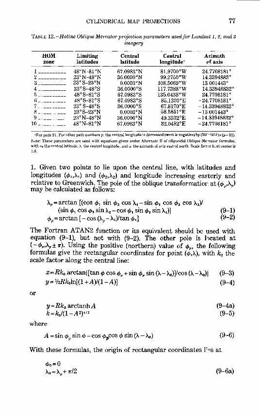
CYLINDRICAL MAP PROJECTIONS 77
TABLE 12.-Hotine Oblique Mercator projection parameters used for Landsa.t 1, 2, and 3 imagery
HOM Limiting Central Central A~imuth zone latitudes latitude longitude' ('{axis
1 ---------- 48°N-81 °N 67.0983°N 81.9700°W 24.7708181° 2 ----------- 23°N-48°N 36.0000°N 99.2750°W 14.3394883° 3 --------~- 23°S-23°N 0.0003°N 108.5069°W 13 001443° 4--------- 23° S-48°8 36.0000°8 117.7388°W 14.33948832° 5 ---------- 48°8-81°8 67.0983°8 135.0438°W 24.7708181° 6 ---------- 48°8-81°8 67.0983°8 85.1220°E -24.7708181° 7 ---------- 23° S-48°8 36.0000°8 67.8170°E -14.33948832° 8 ---------- 23°S-23°N 0.0003°N 58.5851 °E -13.001443° 9 ---------- 23°N-48°N 36.0000°N 49.3532°E -14.33948832°
10 ---------- 48°N-81 °N 67.0983°N 32.0482°E - 24.7708181°
'For path 31. For other path numbers p, the central longitude is decreased (west is negative) by (36('" /25l)x (p- 31).
Note: These parameters are used with equations given under Alternate B of ellipsoidal Oblique Me.-cator formulas, with <Po the central latitude, l\. the central longitude, and u, the azimuth of axis east of north. Scale facbr kn at center is 1.0.
1. Given two points to lie upon the central line, with latitudes and longitudes (c/>~,A..) and (c/>2,:\2) and longitude increasing ea~terly and relative to Greenwich. The pole of the oblique transformatior at (cf>p,A.P) may be calculated as follows:
Ap =arctan [(cos ct>. sin c/>2 cos A..- sin c/>1 cos c/>2 cos :\2)/
(sin c/> 1 cos f/>2 sin :\2 - cos c/>1 sin c/>1 sin :\1)] (9-1) cf>p =arctan [-cos (:\P- A..)ltan ct>.] (9-2)
The Fortran ATAN2 function or its equivalent should be used with equation (9-1), but not with (9-2). The other pole is heated at ( -c/>p,Ap± r). Using the positive (northern) value of cf>p, the following formulas give the rectangular coordinates for point ( c/>,A.), with k0 the scale factor along the central line:
or
x=Rko arctan([tan cf> cos cf>p +sin cf>p sin (A- A.o)]/cos (:\- A.o)) y= 1hRkoln[(1 +A)/(1-A)]
y = Rko arctanh A k= koi(1-A2)t12
where
A =sin cf>p sin c/>- cos cf>pcos c/> sin (:\- A.o)
(9-3)
(9-4)
(9-4a) (9-5)
(9-6)
With these formulas, the origin of rectangular coordinates Fo,s at
(9-6a)
78 MAP PROJECTIONS USED BY THE USGS
and the X axis lies along the central line, x increasing easterl:T. The transformed poles are y equals infinity. 2. Given a central point (c/>c, Ac) with longitude increasing easterly and relative to Greenwich, and azimuth {3 east of north of the central line through (cJ>),), the pole of the oblique transformation at (c/JP, A) may be calculated as follows:
c/>p =arcsin (cos cl>c sin {3) Ap =arctan [- cos{3/(- sin cl>c sin /3)] + Ac
(9-7) (9-8)
These values of cJ>P and AP may then be used in equations (9-3) through (9-6) as before. 3. For an extensive map, c/>p and Ap may be arbitrarily chosen by eye to give the pole for a central line passing through a desired portior of the globe. These values may then be directly used in equations (9-3) through (9-6) without intermediate calculation.
For the inverse formulas, equations {9-1) and (9-2) or (9-7) an-i (9-8) must first be used to establish the pole of the oblique transformation, if it is not known already. Then,
cJ> =arcsin [sin cJ>P tanh (y/Rko) +cos cJ>P sin (x/Rko)/cosh (y!Rko)] (9-9) A= Ao +arctan {Lsin cpp sin (x/Rk0)- cos cpp sinh (y/Rk0)]/cos (x/Rko)} (9-10)
FORMULAS FOR THE ELLIPSOID
These are the formulas provided by Hotine, slightly altered to use a positive eastern longitude (he used positive western longituie), to simplify calculations of hyperbolic functions, and to use symbc1s consistent with those of this bulletin. The central line is a geodesic, or the shortest route on an ellipsoid, corresponding to a great circle route on the sphere.
It is customary to provide rectangular coordinates for the He tine in terms either of (u, v) or (x,y). The (u, v) coordinates are similar in concept to the (x,y) calculated for the foregoing spherical formulas, with u corresponding to x for the spherical formulas, increasing easterh· from the origin along the central line, but v corresponds to - y for the spherical formulas, so that v increases southerly in a direction r~rpendicular to the central line. For the Hotine, x and y are calculatei from (u,v) as "rectified" coordinates with theY axis following the meridian passing through the center point, and increasing northerly as usual, while the X axis lies east and west through the same point. The X and Y axes thus lie in directions like those of the Transverse Mercator, but the scale-factor relationships remain those of the Oblique Mercator.
The normal origin for (u,v) coordinates in the Hotine Obliqu~ Mercator is approximately at the intersection of the central line with the Earth's Equator. Actually it occurs at the crossing of the central line with the equator of the "aposphere," and is, thus, a rather academic location. The "aposphere" is a surface with a constant "total" cur<rature
CYLINDRICAL MAP PROJECTIONS 79
based on the curvature along the meridian and perpendicular thereto on the ellipsoid at the chosen central point for the projectio:rt. The ellipsoid is conformally projected onto this aposphere, then to a sphere, then to a plane. As a result, the Hotine is perfectly conformal, but the scale along the central line is true only at the chosen central point along that line or along a relatively flat elliptiCally shaped line approximately centered on that point, if the scale of the central point i~· arbitrarily reduced to balance scale over the map. The variation in scale along the central line is extremely small for a map extending less than 45 ° in arc, which includes most existing usage of the Hotine. A longer central line suggests the use of a different set of formulas, available as a limiting form of the Space Oblique Mercator projection. On Rosenmund's (1903), Laborde's (1928), and Cole's (1943) versions of the ellipsoidal Oblique Mercator, the central line is a great circle arc on the intermediate conformal sphere, not a geodesic. As on Hotine's version, this central line is not quite true to scale except at one or two chosen points.
The projection constants may be established for the Hotine in one of two ways, as they were for the spherical form. Two desired points, widely separated on the map, may be made to fall on the central line of the projection, or the central line may be given a desired azimuth through a selected central point. Taking these approaches in order:
Alternate A, with the central line passing through two given points. Given:
a and e for the reference ellipsoid. ko = scale factor at the selected center of the map, lying or the central
line. c/Jo =latitude of selected center of the map. (c/J,, At)=latitude and longitude (east of Greenwich is positive) of the
first point which is to lie on the central line. ( c/J2, A2) =latitude and longitude of the second point whicl· is to lie on
the central line. ( ¢, A)= latitude and longitude of the point for which the coordinates
are desired.
There are limitations to the use of variables in these formulas: To avoid indeterminates and division by zero, ¢ 0 or cp, cannot be ± 1r/2, ¢ 1
cannot be zero or equal to c/J2 (although c/J2 may be zero), and ¢ 2 cannot be -1r/2. Neither c/Jo, ¢,,nor c/J2 should be ± 1r/2 in any case, since this would cause the central line to pass through the pole, fo"' which the Transverse Mercator or polar Stereographic would probably be a more suitable choice. A change of 10-7 radian in variables from these special values will permit calculation of an otherwise unsatisfactory condition.
It is also necessary to place both (cp,, A,) and (¢2, A2) on th~ ascending portion, or both on the descending portion, of the central line, relative
80 MAP PROJECTIONS USED BY THE USGS
to the Earth's Equator. That is, the central line should not pass through a maximum or minimum between these two points.
If e is zero, the Hotine formulas give coordinates for the spl,~rical Oblique Mercator.
Because of the involved nature of the Hotine formulas, they are given here in an order suitable for calculation, and in a form eliminating the use of hyperbolic functions as given by Hotine in favor of single calculations of exponential functions to save computer time. The correrDonding Hotine equations are given later for comparison.
B = [1 + e2 cos4 cp0 /(1- e2))1'2
A= aBko(1- e2)
1121(1- e2 sin2 cp0 )
to= tan {'n-/4- cJ>o/2)/[(1- e sin cp0)/(1 + e sin cp0 )]"12
t, =same as (9-13), using cp 1 in place of cp0 •
t2 =same as (9-13), using cp2 in place of cp0 •
D =B(1- e2)
1121[cos cl>o(1- e2 sin2cp0)112]
(9-11) (9-12) (9-13)
(9-14)
If cl>o = 0, D may calculate to slightly less than 1.0 and create a problem in the next step. If D 2 < 1, it should be made 1.
E = [D ± (D2 -1)112]t08
, taking the sign of cp0
H=t, 8
L=t2B F=EIH G=(F-1/F)/2 J = (E2
- LH)/(E2 + LH) P= (L -H)I(L +H) Ao = 112(A. + A2)- arctan {J tan [B(A,- Al)/2]/P}/B 'Yo= arctan {sin [B(A.- Ao)]/GJ ac = arcsin [D sin 'Yo]
(9-15) (9-16) (9-17) (9-18) (9-19) (9-20) (9-21) (9-22) (9-23) (9-24)
To prevent problems when straddling the 180th meridian with A1 and A2, before calculating (9-22), if (A.- A1) < - 180°, subtract 360° fr0m A2. If (A1 -A2)> 180°, add 360° to A2. Also adjust Ao and (>-.1 -Ao) to fall between ± 180° by adding or subtracting 360°. The Fortran ATAN2 function is not to be used for equations (9-22) and (9-23). The above equations (9-11) through (9-24) provide constants for a given map and do not involve a specific point (cp,>-.). Angle ac is the azimuth of tl'~ central line as it crosses latitude cf>o, measured east of north. For pdnt (cp, A), calculate the following:
t =same as equation (9-13), but using cp in place of cf>o.
If cp = ± 1r/2, do not calculate t, but go instead to (9-30). Q=~~ ~~~ S=(Q-1/Q)/2 (9-26) T=(Q+ 1/Q)/2 (9-27) V =sin [B(>-.- >-.o)] (9-28)
CYLINDRICAL MAP PROJECTIONS 81
U = (- V cos 'Yo+ S sin -y0)/T (9-29) V=A In [(1- U)/(1 + U)]/2B (9-30)
Note: If U = ± 1, v is infinite; if cJ> = ± 1r/2, v =(AlB) In tan ( 1rl 4 +-y0/2)
u=A arctan {(S cos 'Yo+ V sin -y0)/cos [B(>..- }..0 )])/B (9-31)
Note: If cos [B(}..-}..0)]=0, U=AB(}..-}..0 ). If c/>= ±7r/2, U=A¢/B.
Care should be taken that (>..- }..0) has 360° added or subtracted, if the 180th meridian falls between, since multiplication by B eliminates automatic correction with the sin or cos function.
The scale factor:
k=A cos (Bu/A)(1- e2 sin 2¢)112/{a cos¢ cos [B(>..- A0)]} (9-32)
If "rectified" coordinates (x, y) are desired, with the origin at a distance (xo,Yo) from the origin of the (u,v) coordinates, relative to the (X, Y) axes (see fig. 13):
X= V COS ac + U sin ac + Xo
y = u cos ac- v sin ac +Yo (9-33) (9-34)
The formulas given by Hotine and essentially repeated in Thomas (1952, p. 7-9), modified for positive east longitude, u and v increasing in the directions shown in figure 13, and symbols consistent with the above, relate to the foregoing formulas as follows: 3
Equivalent to (9-11):
,p = e2/(1- e2)
B = (1 + ff2 COS 4¢ 0)'/z
Equivalent to (9-12):
R'o = a(1- e2)/(1- e2 sin 2¢0)3' 2
No= a/(1- e2 sin 2¢0)1' 2
A =Bko(R'oNo)lf2
Other formulas:
ro =No cos c/>o ~n =In {tan (7r/4 + ¢)2)[(1- e sin cPn)/(1 + e sin cPn)]e12
}
Note: ~n is equivalent to ( -ln tn) using equation (9-13).
C= ± arccosh (Air0)-B~o
Note: Cis equivalent to ln E, where E is found from equation (9-15); D, from (9-14), is (Afro).
tan [IhB(>-.1 + >..2)- B>..o] = tan (lhB(}..l ->..2)] tanh (112B(~~ +~2)+C]
tanh [ 112B(~~- ~2)]
'llotirw ust•s positiVl' Wl·st longrtude, .r corresponding to 11 here, and y corresponding to -t• here. Thomas uses positivl' west longitwll'. yeorrespondmg to 11 here, and .17 corresponding to - '' here. In calculations of Alaska zone 1, Wl•st longitude is positive, hut 11 and I' agret' with u and t•. respel'tively, here.
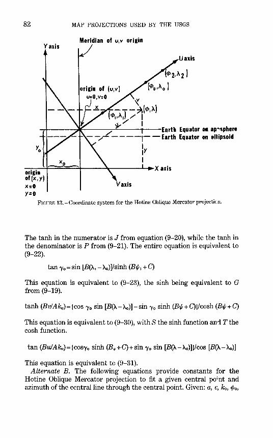
82 MAP PROJECTIONS USED BY THE USGS
Meridian of u,v origin Yaxis
Uaxis
origin of (u,v) u:O,v:O v
t ~ -~ --~(<t>,)t) ( <t>., A I ) / I
/ I _,...t.---_,.F----/-.:;.~----+--Earth Equator on ap~$phere
- -,....- - ---~- -Earth Equator on ellipsoid
ly I Xo
~~~=::::::::=~--~~---..L....,..X axis origin of(x,y) X:O Y=O
Vaxis
FIGURE 13.-Coordinate system for the Hotine Oblique Mercator projecticn.
The tanh in the numerator is J from equation (9-20), while the tanh in the denominator is P from (9-21). The entire equation is equivalent to (9-22).
tan 'Yo= sin [B(A.1- A.o)]/sinh (Bt/;1 +C)
This equation is equivalent to (9-23), the sinh being equivalent to G from (9-19).
tanh (Bv/Ak0)={cos 'Yo sin [B(A.-A.0)]-sin 'Yo sinh (Bt/;+C))/cosh (Bt/;+C)
This equation is equivalent to (9-30), with S the sinh function ani T the cosh function.
tan (Bu/Ako)={COS')'o sinh (B~+C)+sin 'Yo sin [B(A.-A.o)]}/cos [B(A.-A.o)]
This equation is equivalent to (9-31). Alternate B. The following equations provide constants for the
Hotine Oblique Mercator projection to fit a given central po~nt and azimuth of the central line through the central point. Given: a, e, ko, cf>o,
CYLINDRICAL MAP PROJECTIONS 83
and (c/>, A) as for alternate A, but instead of (cl>t, At) and (ct>2, A2), Ac and ac are given,
where
(c/>o, Ac)=latitude and longitude (east of Greenwich is positiv~), respectively, of the selected center of the map, falling C''l the central line.
ac =angle of azimuth east of north, for the central line a~ it passes through the center of the map ( cl>o, Ac).
Limitations: cl>o cannot be zero or ± 1rl2, and the central line cannot be at a maximum or minimum latitude at c/>o. If e = 0, these for~ulas also give coordinates for the spherical Oblique Mercator. As witl' alternate A, these formulas are given in the order of calculation and are modified to minimize exponential computations. Several of t~ese equations are the same as some of the equations for alternate A:
B = [1 + e2 cos4 c/>o/(1- e2))1'2 (9-11) A = aBko (1- e2)112/(1- e sin2 cl>o) (9-12) to= tan( 7r/4- c/>o/2)/[(1- e sin cl>o)/(1 + e sin c/>o)]e12 (9-13) D =B(1- e2
)1121[ cos cl>o {1- e2 sin2 cl>o)112] {9-14)
If c/>o=O, D may calculate to slightly less than 1.0 and create a problem in the next step. If D 2 < 1, it should be made 1.
F=D±(D2-1)112, taking the sign of c/>0
E=Fto8
G=(F-1/F)/2 'Yo= arcsin (sin a)D) Ao = Ac- [arcsin (G tan 'Yo)]/B
(9-35) (9-36) (9-19) (9-37) (9-38)
The values of u and v for center point (c/>o, Ac) may be calculated directly at this point:
u(<P •• ~> = ±(AlB) arctan [(D2 -1)1'
2/cos ac], taking the sign of c/>o. (9-39) V(q,.,>.,)=O
These are the constants for a given map. Equations (9-2F) through (9-32) for alternate A may now be used in order, following calculation of the above constants.
The inverse equations for the Hotine Oblique Mercator prc.;ection on the ellipsoid may be shown with few additional formulas. To determine c1> and A from x andy, or from u and v, the same parameters of the map must be given, except for c1> and A, and the constants of th~ map are found from the above equations (9-11) through (9-24) for alternate A or (9-11) through (9-38) for alternate B. Then, if X andy are given in
84 MAP PROJECTIONS USED BY THE USGS
accordance with the definitions for the forward equations, the:r must first be converted to (u, v):
V=(X-Xo) cos Ole- (Y-Yo) sin Ole U=(Y-Yo) cos Ot.e+(X-Xo) sin Ole
(9-40) (9-41)
If (u, v) are given, or calculated as just above, the following steps are performed in order:
Q' = e-(Bv/A) (9-42)
where e = 2. 71828 ... , the base of natural logarithms
S' = (Q' -1/Q')/2 (9-43) (9-44) (9-45) (9-46)
T' = (Q' + 1/Q')/2 V' =sin (Bu/A) U =(V'cos 'Yo+S' sin 'Yo)IT'
t= (E/[(1 + U)/(1- U))1' 2l 118 (9-47)
But if U = ± 1, cJ> = ± 90°, taking the sign of U, A may be called Ao, and equations (7 -9) and (9-48) below are omitted.
cJ> = 1r/2 -2 arctan (t[(1- e sin cJ>)/(1 +e sin cJ>)]e' 2 l (7-9)
Equation (7-9) is solved by iteration, using cJ> =(7r/2- 2 arctan t) as the first trial cJ> on the right side, and using the successive calculatio'1s of cJ>
on the left side as successive values of cJ> on the right side, until the change in cJ> is less than a chosen convergence value.
A=Ao-arctan [(S' cos 'Yo- V' sin 'Yo)/cos (Bu/A)]IB (9-48)
Since the arctan (found as the ATAN2 function) is divided by B, it is necessary to add or subtract 360° properly, before the division.
To avoid the iteration, the series (3-5) may be used with (7-13) in place of (7-9):
c/>=x+(e2/2+5e4/24+e6/12+ ... ) sin 2x+(7e4/48+29e6/240+ ... ) sin 4x + (7 e6/120 + . . . ) sin 6x + . . . (3-5)
where
x = 1r/2- 2 arctan t (7-13)
The equivalent inverse equations as given by Hotine are as follows, following the calculation of constants using the same formulas a" those given in his forward equations:
tan [B(A-Ao)]=[sin 'Yo sin (Bu/A)+cos 'Yo sinh (Bv/A)]/cos (B~·lA) tanh (B~+C)=[cos 'Yo sin (Bu/A)-sin 'Yo sinh (Bv/A)]/cosh (BdA)

10. MILLER CYLINDRICAL PROJECTION
SUMMARY
• Neither equal-area nor conformal. • Used only in spherical form. • Cylindrical. • Meridians and parallels are straight lines, intersecting at right angles. • Meridians are equidistant; parallels spaced farther apart away from Equator. • Poles shown as lines. • Compromise between Mercator and other cylindrical projections. • Used for world maps. • Presented by Miller in 1942.
HISTORY AND FEATURES
The need for a world map which avoids some of the scale exaggeration of the Mercator projection has led to some commonly U"ed cylindrical modifications, as well as to other modifications whicl:t are not cylindrical. The earliest common cylindrical example was developed by Rev. James Gall of Edinburgh about 1855 (Gall, 1885, p. 119-123). His meridians are equally spaced, but the parallels are spaced at increasing intervals away from the Equator. The parallels of latitude ar~~ actually projected onto a cylinder wrapped about the sphere, but cutting it at lats. 45 o N. and S., the point of perspective being a point on the Equator opposite the meridian being projected. It is used in several British atlases, but seldom in the United States. Gall's projection is neither conformal nor equal-area, but has a blend of various features. Unlike the Mercator, Gall's shows the poles as lines running f~ross the top and bottom of the map.
What might be called the American version of Gall's projection is the Miller Cylindrical projection (fig. 14), presented in 1942 b:T Osborn Maitland Miller (1897-1979) of the American GeographicaJ Society, New York (Miller, 1942). Born in Perth, Scotland, and ed'Icated in Scotland and England, Miller came to the Society in 1922. There he developed several improved surveying and mapping techniques. An expert in aerial photography, he developed techniques for converting high-altitude photographs into maps. He led or joined several expeditions of explorers and advised leaders of others. He retired in 1968, having been best known to cartographers for several map pr~1jections, including the Bipolar Oblique Conic Conformal, the Prolated Stereographic, and especially his Cylindrical projection.
Miller had been asked by S. Whittemore Boggs, Geograpl,~r of the U.S. Department of State, to study further alternative:~ to the
85
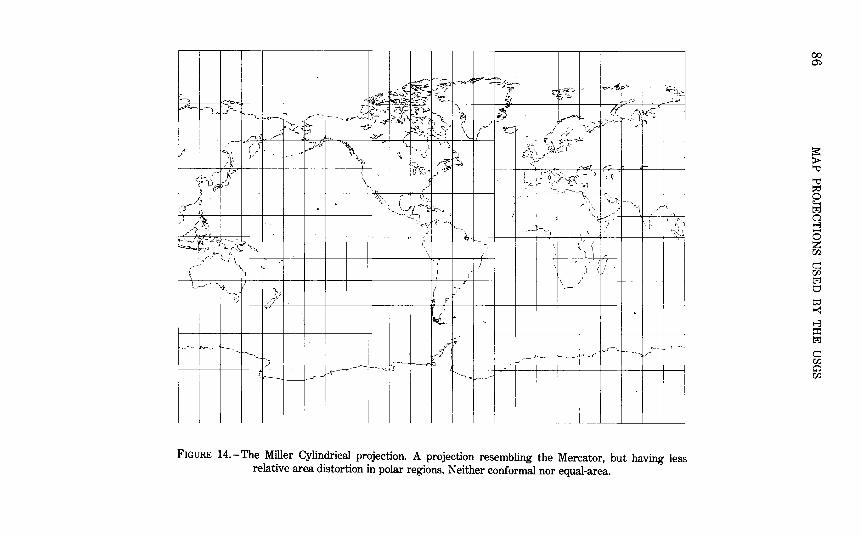
b 1.0'h iv;_~ ~·~~~ -.... ~1-"'Jyp ~";~ - r--~ " oq,~ ~h - .., --->"\.,t •• ¢1~~ ~ ~ ~/ f-:::o? __:_:;=
•l_ev--~ ~ ~p~-~ \ ~ # -:?' l--os----~ r-""-t---- -~ ~);;> ;\ p.:~'--~ ~ ~ ..- ~ ('~~ ~ ,~<>- -z~ v , , ) ~ tJ .~f- v· r-- -, DA- r---'" 1, r. .n ~ ~ b .:y- ?!:"'J0,,~j':,_~~"' \ .. ! t ' C ILf ll;:l'- _,
.~ ""xi ... (,} --- --~A· "~~- ~ ; '~- --u~ "'"\~ i£·. -s~ :_!J /~. I ~ 0~ /~~ ~~~f
J,~ / r r: 1 1 u ~'f . ~ . .r? ~- i-'ru.t;:::~ \ ~ ~~-:a·-w>..--);~' 1 \) .JOO r- LC~) 'It\ «l
~-""b ~'il.'\ ( \]-, ----;J-:c'-; i_t-_·---p'-~~-=f1~,.\rr-' --+,..----1-----1--_j__J <.o h , 1., h~- 1,- "'--"=r-
r---. '·-'II ~=· "' '1 1
) ' . l'i) ~~L. ,~~ I - - I ,t· ,-r~ ( ' • ~) ~, ~ ' f; '• (, ' 'i(' ~__J 1\i"''""'f).....___. 0:.\ \ <;>· -,] I \ ·+t-----1--+--f-'~:~\~~ ~- ,,. ;,_ _--[' . '""· \ l \ ~
(
I '-._] \., •• '-/ / I) ~'I I I I I \ j I ' .
'l~-r '!, 1/ ')..., I) ~i' ' r ~0 JF I~ ~,I
~ ' ~
!'------~ />v-..r-~ ~];0-!'--.... J • ~_,--,__ ~.--1--r -~
~ tJ ---~f-._ r'r ---< Fl -~- )-------- r J ~--~--c--_- ___..r- p- -----.~ -- -
-- --- ___ _L______L _ _j____l_ __ _l____
FIGURE 14.-The Miller Cylindrical projection. A projection resembling the Mercator, but having less relative area distortion in polar regions. Neither conformal nor equal-area.
00 ~
s:: > "t1
"t1 ~ 0 t;J C':l ~ -0 z w. ~ w. tzj t;:;
O::l ~
~ ::I:: tzj
~ w. CJ w.
CYLINDRICAL MAP PROJECTIONS 87
Mercator, Gall's, and other cylindrical world maps. In his pres~ntation, Miller listed four proposals, but the one he preferred, and the one used, i8 a fairly simple mathematical modification of the Mercator projection. Like Gall's, it shows visible straight lines for the poles, inc':"easingly spaced parallels away from the Equator, equidistant meridians, and is not equal-area, equidistant along meridians, nor conformal. "\V"hile the standard parallels, or lines true to scale and free of distortion, on Gall's are at lats. 45° N. and S., on the Miller only the Equator is standard. Unlike Gall's, Miller's is not a perspective projection.
The Miller Cylindrical projection is used for world mar~ and in several atlases, including the National Atlas of the Unitl3d States (USGS, 1970, p. 330-331).
As Miller (1942) stated, "the practical problem considered here is to find a system of spacing the parallels of latitude such that an a~ceptable balance is reached between shape and area distortion. By an 'acceptable' balance is meant one which to the uncritical eye does no~ obviously depart from the familiar shapes of the land areas as depicted by the Mercator projection but which reduces areal distortion as far as possible under these conditions * * *. After some experimenting, the [Modified Mercator (b)] was judged to be the most suitabl~ for Mr. Boggs's purpose * * *."
FORMULAS FOR THE SPHERE
Miller's spacings of parallels from the Equator are the same as if the Mercator spacings were calculated for 0.8 times the respective latitudes, with the result divided by 0.8. As a result, the S"1acing of parallels near the Equator is very close to the Mercator arrangement.
The forward formulas, then, are as follows:
X=R("A-"Ao) y=R[ln tan (1r/4 + 0.4cJ>)]/0.8
or
y=R[arctanh (sin 0.8cJ>)]/0.8
The scale factor, using equations (4-2) and (4-3),
h=sec 0.8cJ> k=seccJ>
The maximum angular deformation w, from equation ( 4-9),
sin 112w=(cos 0.8c/>-cos cJ>)/(cos 0.8cJ>+cos c/>)
(10-1) (10-2)
(10-2a)
(10-3) (10-4)
(10-5)
The X axis lies along the Equator, x increasing easterly. The Y axis lies along the central meridian "Ao, y increasing northerly. If () - "Ao) lies
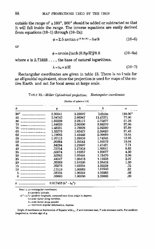
88 MAP PROJECTIONS USED BY THE USGS
outside the range of ± 180°, 360° should be added or subtracted so that it will fall inside the range. The inverse equations are easily derived from equations (10-1) through (10-2a):
<P = 2.5 arctan e(o.sytR>- S1r/8
or
<P =arcsin [tanh (0.8y/R)]/0.8
where e is 2. 71828 ... , the base of natural logarithms.
'A='Ao+x!R
(10-6)
(10-6a)
(10-7)
Rectangular coordinates are given in table 13. There is no l'~sis for an ellipsoidal equivalent, since the projection is used for maps of the entire Earth and not for local areas at large scale.
TABLE 13. -Miller Cylindrical projection: Rectangular coordinates
90° --------------85 ---------------80 ---------------75 ---------------70 ---------------65 ---------------60 ---------------55 ---------------50 ---------------45 ---------------40 ---------------35 ---------------30 ---------------25 ---------------20 ---------------15 ---------------10 ---------------5 ---------------0 ---------------
y
2.30341 2.04742 1.83239 1.64620 1.48131 1.33270 1.19683 1.07113
.95364
.84284
.73754
.63674
.53962
.44547
.35369
.26373
.17510
.08734
.00000
[Radius of sphere= 1.0]
h
3.23607 2.66947 2.28117 2.00000 1.78829 1.62427 1.49448 1.39016 1.30541 1.23607 1.17918 1.13257 1.09464 1.06418 1.04030 1.02234 1.00983 1.00244 1.00000
X ---------------- 0.017 453 (A 0 - Xc, 0
)
Note: x, y=rectangular coordinates. <1> =geodetic latitude.
(>. o- >.. 0 ) =geodetic longitude, measured east from origin in degrees. h =scale factor along meridian. k =scale factor along parallel. w =maximum angular deformation, degrees.
k
Infinite 11.47371
5.75877 3.86370 2.92380 2.36620 2.00000 1.74345 1.55572 1.41421 1.30541 1.22077 1.15470 1.10338 1.06418 1.03528 1.01543 1.00382 1.00000
w
180.00° 77.00 51.26 37.06 27.89 21.43 16.64 12.95 10.04 7.71 5.82 4.30 3.06 2.07 1.30
.72
.32
.08
.00
Origin of coordinates at intersection of Equator with>.,. X axis increases east, Y axis increases north. For southern (negative) <1>, reverse sign of y.
• Cylindrical.
11. EQUIDISTANT CYLINDRICAL PROJECTION
SUMMARY
• Neither equal-area nor conformal. • Meridians and parallels are equidistant straight lines, intersecting at right angles. • Poles shown as lines. • Used for world or regional maps. • Very simple construction. • Used only in spherical form. • Presented by Eratosthenes (B.C.) or Marinus (A.D. 100).
HISTORY AND FEATURES
While the Equidistant Cylindrical projection is listed last among the cylindricals because of its limited use by the USGS and generally limited value, it is probably the simplest of all map projecti0ns to construct and one of the oldest. The meridians and paralhls are all equidistant straight parallel lines, the two sets crossing at ri:-rht angles.
The projection originated probably with Eratosthenes (275?-195? B.C.), the scientist and geographer noted for his fairly accurate measure of the size of the Earth. Claudius Ptolemy credited Marin us of Tyre with the invention about A.D. 100 stating that, whr~ Marinus had previously evaluated existing projections, the latter had chosen "a manner of representing the distances which gives the worst results of all." Only the parallel of Rhodes (lat. 36° N.) was made true to scale on the world map, which meant that the meridians were spac(ld at about four-fifths of the spacing of the parallels for the same degr9e interval (Keuning, 1955, p. 13).
Ptolemy approved the use of the projection for maps of smaller areas, however, with spacing of meridians to provide correct scale along the central parallel. All the Greek manuscript maps for the Geographia, dating from the 13th century, use the Ptolemy modi:ficathn. It was used for some maps until the eighteenth century, but is now used primarily for a few maps on which distortion is considered less important than the ease of displaying special information. The projection is given a variety of names such as Equidistant Cylindrical, Rectangular, La Carte Parallelogrammatique, Die Rechteckige Plattkarte, and Equirectangular (Steers, 1970, p. 135-136). It was called the projection of Marinus by Nordenskiold (1889). If the Equator is made the standard parallel, true to scale and free of
distortion, the meridians are spaced at the same distan~es as the parallels, and the graticule appears square. This form is often called the Plate Carree or the Simple Cylindrical projection.
89
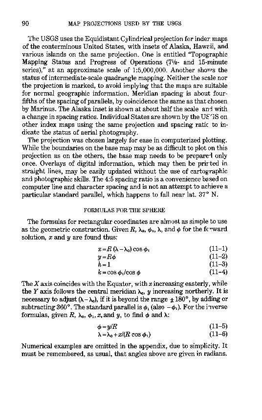
90 MAP PROJECTIONS USED BY THE USGS
The USGS uses the Equidistant Cylindrical projection for indeY maps of the conterminous United States, with insets of Alaska, Hawr.ii, and various islands on the same projection. One is entitled "Topographic Mapping Status and Progress of Operations {71/2- and 15-minute series)," at an approximate scale of 1:5,000,000. Another shows the status of intermediate-scale quadrangle mapping. Neither the scale nor the projection is marked, to avoid implying that the maps are suitable for normal geographic information. Meridian spacing is about fourfifths of the spacing of parallels, by coincidence the same as that chosen by Marin us. The Alaska inset is shown at about half the scale an1 with a change in spacing ratios. Individual States are shown by the UFr;s on other index maps using the same projection and spacing ratic to indicate the status of aerial photography.
The projection was chosen largely for ease in computerized plotting. While the boundaries on the base map may be as difficult to plot on this projection as on the others, the base map needs to be prepare1 only once. Overlays of digital information, which may then be prirted in straight lines, may be easily updated without the use of cartographic and photographic skills. The 4:5 spacing ratio is a convenience based on computer line and character spacing and is not an attempt to achieve a particular standard parallel, which happens to fall near lat. 37° N.
FORMULAS FOR THE SPHERE
The formulas for rectangular coordinates are almost as simple to use as the geometric construction. Given R, Ao, c/>1, A, and cp for the fcrward solution, x and-Y are found thus:
X=R (A-Ao) COS c/>1 y=Rc/> h=1 k =cos cl>t/cos cp
(11-1) (11-2) (11-3) (11-4)
The X axis coincides with the Equator, with x increasing easterly, while theY axis follows the central meridian Ao, y increasing northerly. It is necessary to adjust (A.- Ao), if it is beyond the range ± 180 °, by adding or subtracting 360°. The standard parallel is c/>1 (also - cl>t). For the i"lverse formulas, given R, Ao, cp., x, and y, to find cp and A.:
cJ>=yiR A.= Ao + xi(R cos cl>t)
(11-5) (11-6)
Numerical examples are omitted in the appendix, due to simplicity. It must be remembered, as usual, that angles above are given in radians.
CONIC MAP PROJECTIONS
Cylindrical projections are used primarily for complete world maps, or for maps along narrow strips of a great circle arc, such as the Equator, a meridian, or an oblique great circle. To show a region for which the greatest extent is from east to west in the temperate zones, conic projections are usually preferable to cylindrical projections.
Normal conic projections are distinguished by the use of arcs of concentric circles for parallels of latitude and equally spaced straight radii of these circles for meridians. The angles between the meridians on the map are smaller than the actual differences in longitude. T~·e circular arcs may or may not be equally spaced, depending on the projection. The Polyconic projection and oblique conic projections have characteristics different from these.
The name "conic" originates from the fact that the more e:1ementary conic projections may be derived by placing a cone on the tor of a globe representing the Earth, the apex or tip in line with the r.xis of the globe, and the sides of the cone touching or tangent to the globe along a specified "standard" latitude which is true to scale and with'lut distortion (see fig. 1). Meridians are drawn on the cone from the apex to the points at which the corresponding meridians on the glob~ cross the standard parallel. Other parallels are then drawn as arcs centered on the apex in a manner depending on the projection. If the cone is cut along one meridian and unrolled, a conic projection results. A secant cone results if the cone cuts the globe at two specified parallels. Meridians and parallels can be marked on the secant cone sonewhat as above, but this will not result in any of the common conic projections with two standard parallels. They are derived from vario•:ts desired scale relationships instead, and the spacing of the meridians as well as the parallels is not the same as the projection onto a secant cone.
There are three important classes of conic projections: tJ·~ equidistant (or simple), the conformal, and the equal-area. The Equidistant Conic, with parallels equidistantly spaced, originated in a ruiimentary form with Claudius Ptolemy. It eventually developed into commonly used present-day forms which have one or two standarc parallels selected for the area being shown. It is neither conformal nor equalarea, but north-south scale along all meridians is correct, ard the projection can be a satisfactory compromise for errors in shape, scale, and area, especially when the map covers a small area. It is prirrarily used in the spherical form, although the ellipsoidal form is available and useful. The USGS uses the Equidistant Conic in an approximate form
91

92 MAP PROJECTIONS USED BY THE USGS
for a map of Alaska, identified as a "Modified Transverse Mercator" projection, and also in the limiting equatorial form: the Equidistant Cylindrical. Both are described earlier.
The Lambert Conformal Conic projection with two standard parallels is used frequently for large- and small-scale maps. The paralhls are more closely spaced near the center of the map. The Lambert has also been used slightly in the oblique form. The Albers Equal-Arer. Conic with two standard parallels is used for sectional maps of the U.S. and for maps of the conterminous United States. The Albers parallels are spaced more closely near the north and south edges of the map. There are some conic projections, such as perspective conics, which do not fall into any of these three categories, but they are rarely used.
The useful conic projections may be geometrically constructed only in a limited sense, using polar coordinates which must be calc'llated. After a location is chosen, usually off the final map, for the cente .... of the circular arcs which will represent parallels of latitude, meridians are constructed as straight lines radiating from this center and spaced from each other at an angle equal to the product of the cone constant times the difference in longitude. For example, if a 10° grat~n.ule is planned, and the cone constant is 0.65, the meridian lines are sp~ced at 10° times 0.65 or 6.5°. Each parallel of latitude may then be drawn as a circular arc with a radius previously calculated from formulas for the particular conic projection.
• Conic.
12. ALBERS EQUAL-AREA CONIC PROJECTION
SUMMARY
• Equal-Area. • Parallels are unequally spaced arcs of concentric circles, more closely spaced at the
north and south edges of the map. • Meridians are equally spaced radii of the same circles, cutting parall ~ls at right
angles. • There is no distortion in scale or shape along two standard parallels, rormally, or
along just one. • Poles are arcs of circles. • Used for equal-area maps of regions with predominant east-west expanse, especially
the conterminous United States. • Presented by Albers in 1805.
HISTORY
One of the most commonly used projections for maps of the conterminous United States is the equal-area form of the conic projen.tion, using two standard parallels. This projection was first pres~nted by Heinrich Christian Albers (1773-1833), a native of Liineburg, Germany, in a German periodical of 1805 (Albers, 1805; Bona~ker and Anliker, 1930). The Albers projection was used for a German map of Europe in 1817, but it was promoted for maps of the United States in the early part of the twentieth century by Oscar S. Adams of the Coast and Geodetic Survey as "an equal-area representation that is a.s good as any other and in many respects superior to all others" (Adams, 1927, p. 1).
FEATURES AND USAGE
The Albers is the projection exclusively used by the USGP for sectional maps of all 50 States of the United States in the National Atlas of 1970, and for other U.S. maps at scales of 1:2,500,000 anc smaller. The latter maps include the base maps of the United States issued in 1961, 1967, and 1972, the Tectonic Map of the United States (1962), and the Geologic Map of the United States (1974), all at 1:Z,500,000. The USGS has also prepared a U.S. base map at 1:3,168,000 (1 inch=50 miles).
Like other normal conics, the Albers Equal-Area Conic rrojection (fig. 15) has concentric arcs of circles for parallels and equally spaced radii as meridians. The parallels are not equally spaced, but they are farthest apart in the latitudes between the standard parallels and closer together to the north and south. The pole is not the center of the circles, but is normally an arc itself.
93
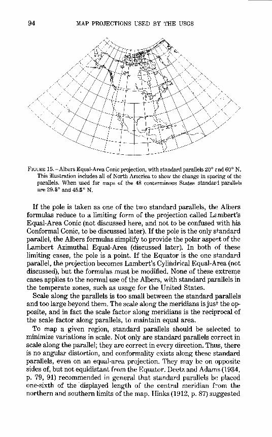
94 MAP PROJECTIONS USED BY THE USGS
FIGURE 15.-Albers Equal-Area Conic projection, with standard parallels 20° G.nd 60° N. This illustration includes all of North America to show the change in spacing of the parallels. When used for maps of the 48 conterminous States standard parallels are 29.5° and 45.5° N.
If the pole is taken as one of the two standard parallels, the Albers formulas reduce to a limiting form of the projection called L2.mbert's Equal-Area Conic (not discussed here, and not to be confused with his Conformal Conic, to be discussed later). If the pole is the only standard parallel, the Albers formulas simplify to provide the polar aspect of the Lambert Azimuthal Equal-Area (discussed later). In both of these limiting cases, the pole is a point. If the Equator is the one standard parallel, the projection becomes Lambert's Cylindrical Equal-Area (not discussed), but the formulas must be modified. None of these extreme cases applies to the normal use of the Albers, with standard parallels in the temperate zones, such as usage for the United States.
Scale along the parallels is too small between the standard parallels and too large beyond them. The scale along the meridians is just. the opposite, and in fact the scale factor along meridians is the reciprocal of the scale factor along parallels, to maintain equal area.
To map a given region, standard parallels should be selected to minimize variations in scale. Not only are standard parallels correct in scale along the parallel; they are correct in every direction. Thus, there is no angular distortion, and conformality exists along these standard parallels, even on an equal-area projection. They may be on opposite sides of, but not equidistant from the Equator. Deetz and Adams (1934, p. 79, 91) recommended in general that standard parallels be placed one-sixth of the ·displayed length of the central meridian f 4 om the northern and southern limits of the map. Hinks (1912, p. 87) suggested
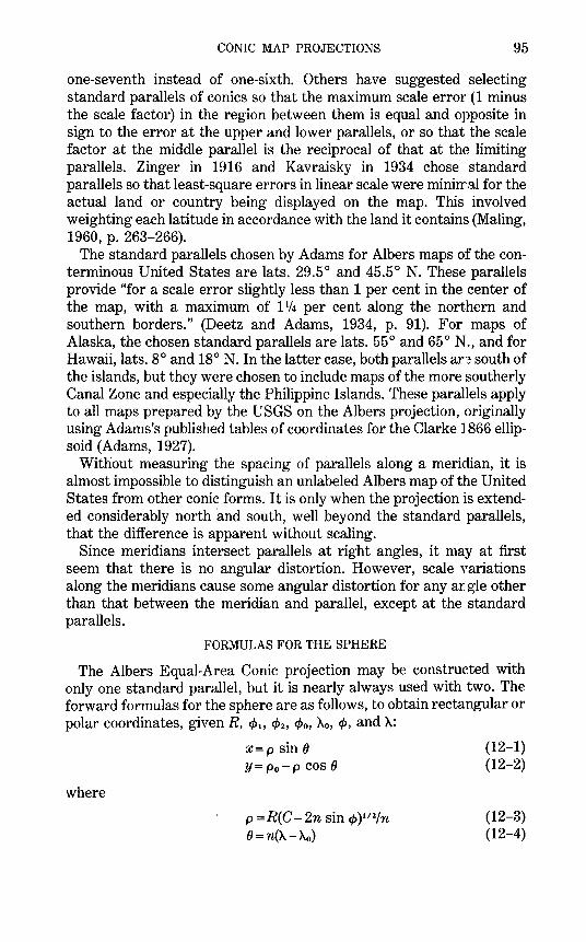
CONIC MAP PROJECTIONS 95
one-seventh instead of one-sixth. Others have suggested selecting standard parallels of conics so that the maximum scale error (1 minus the scale factor) in the region between them is equal and opposite in sign to the error at the upper and lower parallels, or so that the scale factor at the middle parallel is the reciprocal of that at the limiting parallels. Zinger in 1916 and Kavraisky in 1934 chose standard parallels so that least-square errors in linear scale were minirral for the actual land or country being displayed on the map. This involved weighting each latitude in accordance with the land it contains (Maling, 1960, p. 263-266).
The standard parallels chosen by Adams for Albers maps of the conterminous United States are lats. 29.5° and 45.5° N. These parallels provide "for a scale error slightly less than 1 per cent in the center of the map, with a maximum of 11/4 per cent along the northern and southern borders." (Deetz and Adams, 1934, p. 91). For maps of Alaska, the chosen standard parallels are lats. 55° and 65° N., and for Hawaii, lats. 8 o and 18 o N. In the latter case, both parallels ar~~ south of the islands, but they were chosen to include maps of the more southerly Canal Zone and especially the Philippine Islands. These parallels apply to all maps prepared by the USGS on the Albers projection, originally using Adams's published tables of coordinates for the Clarke 1 866 ellipsoid (Adams, 1927).
Without measuring the spacing of parallels along a meridian, it is almost impossible to distinguish an unlabeled Albers map of the United States from other conic forms. It is only when the projection is extended considerably north and south, well beyond the standard parallels, that the difference is apparent without scaling.
Since meridians intersect parallels at right angles, it may at first seem that there is no angular distortion. However, scale yariations along the meridians cause some angular distortion for any all gle other than that between the meridian and parallel, except at the standard parallels.
FORMULAS FOR THE SPHERE
The Albers Equal-Area Conic projection may be constructed with only one standard parallel, but it is nearly always used with two. The forward formulas for the sphere are as follows, to obtain rectangular or polar coordinates, given R, c/>1, c/>2, c/>o, Ao, ¢, and A:
where
X=p sin 0 Y= p0 - p cos 0
p =R(C- 2n sin ¢) 112/n O=n{A-Ao)
(12-1) (12-2)
(12-3) (12-4)
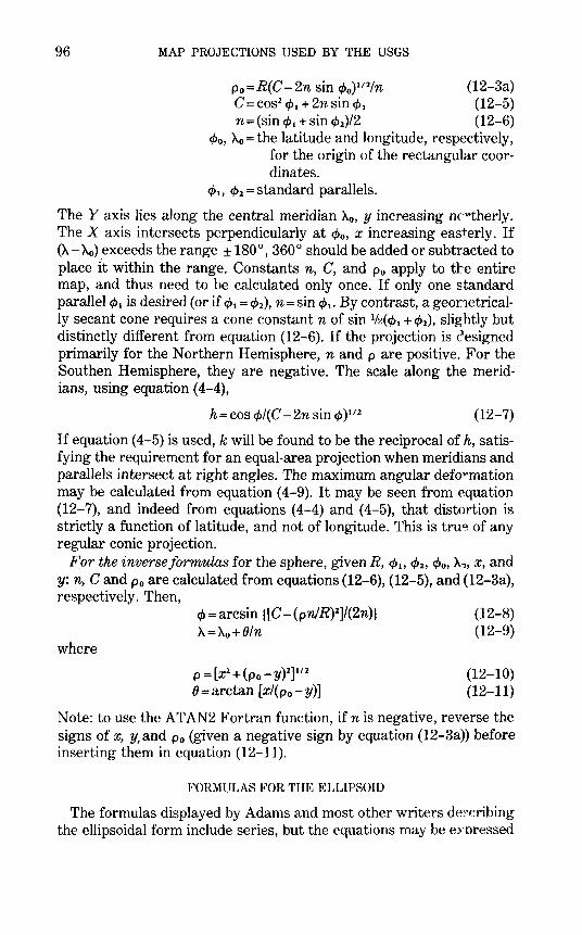
96 MAP PROJECTIONS USED BY THE USGS
Po =R(C- 2n sin ~0) 112/n (12-3a) C = cos2 ~. + 2n sin ~ 1 (12-5) n =(sin ~1 +sin ~2)/2 (12-6)
~o, Ao = the latitude and longitude, respectively, for the origin of the rectangular coordinates.
~1, </>2 =standard parallels.
The Y axis lies along the central meridian Ao, y increasing ncrtherly. The X axis intersects perpendicularly at ~0, x increasing easterly. If (A- Ao) exceeds the range ± 180°, 360° should be added or subtracted to place 1t within the range. Constants n, C, and Po apply to tre entire map, and thus need to be calculated only once. If only one standard parallel </>1 is desired (or if~. = ~2), n =sin ~ •. By contrast, a geometrically secant cone requires a cone constant n of sin 112(~ 1 + ¢ 2), slightly but distinctly different from equation (12-6). If the projection is c1esigned primarily for the Northern Hemisphere, nand p are positive. For the Southen Hemisphere, they are negative. The scale along the meridians, using equation (4-4),
h =cos ~/(C- 2n sin~ )112 (12-7)
If equation ( 4-5) is used, k will be found to be the reciprocal of h, satisfying the requirement for an equal-area projection when meridians and parallels intersect at right angles. The maximum angular defo-rmation may be calculated from equation ( 4-9). It may be seen from equation (12-7), and indeed from equations ( 4-4) and ( 4-5), that distortion is strictly a function of latitude, and not of longitude. This is tru~ of any regular conic projection.
For the inverse formulas for the sphere, given R, ¢ 1, ~2, ~0 , A,1, x, and y: n, C and p0 are calculated from equations (12-6), (12-5), and (12-3a), respectively. Then,
where
~=arcsin {[C-(pn/R)2]/(2n)} A=Ao+Oin
p = [xz + (po _ y)2)ll2 O=arctan [xl(po-Y)]
(12-8) (12-9)
(12-10) (12-11)
Note: to use the ATAN2 Fortran function, if n is negative, reverse the signs of x, y, and Po (given a negative sign by equation (12-3a)) before inserting them in equation (12-11).
FORMULAS FOR THE ELLIPSOID
The formulas displayed by Adams and most other writers de2~ribing the ellipsoidal form include series, but the equations may be exnressed
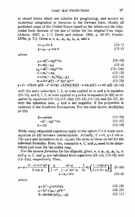
CONIC MAP PROJECTIONS 97
in closed forms which are suitable for programing, and involve no numerical integration or iteration in the forward form. Nearly all published maps of the United States based on the Albers m:e the ellipsoidal form because of the use of tables for the original htse maps. (Adams, 1927, p. 1-7; Deetz and Adams, 1934, p. 93-9~; Snyder, 1979a, p. 71). Given a, e, c/> 1, c/>1, c/>0 , Ao, c/>, and A:
where
X= p sin() y= p0 - p cos 8
(12-1) (12-2)
P = a(C -nq)1'1/n (12-12) 8 = n(A- Ao) (12-4)
p0 =a( C- nq0)111/n (12-12a) C=m1
1 +nq1 (12-13) n=(m~1 -m11)/(q1-q1) (12-14) m =cos cf>/(1- e2 sin1 cf> )111 (12-15)
q=(1-e1){sin ¢/(1-e1 sin1¢)-[11(2e)] ln[(1-e sin ¢)/(1+e sin¢)]) (3-12)
with the same subscripts 1, 2, or none applied tom and cJ> in equation (12-15), and 0, 1, 2, or none applied to q and cJ> in equation (3-12), as required by equations (12-12), (12-12a), (12-13), (12-14), and (12-17). As with the spherical case, p and n are negative, if the projection is centered in the Southern Hemisphere. For the scale factor, modifying (4-25):
k=pnlam =(C-nq)1121m
h= llk
(12-16) (12-17) (12-18)
While many ellipsoidal equations apply to the sphere if e is made zero, equation (3-12) becomes indeterminate. Actually, if e=O, q=2 sin¢. The axes and limitations on (A- Ao) are the same as those st2.ted for the spherical formulas. Here, too, constants n, C, and po need to be determined just once for the entire map.
For the inverse formulas for the ellipsoid, given, a, e, ¢., c/>1, cl>o, Ao, x, andy: n, C, and p0 are calculated from equations (12-14), (12-13), and (12-12a), respectively. Then,
cP = cP + (1- e1 sin2 ¢)2 [_q__ sin cJ> +-1-ln ( 1- e sin cJ> )] (3_16)
2 cos ct> 1 - e2 1 - e2 sin 2 cJ> 2e 1 + e sin cJ>
where
A= Ao + 8/n (12-9)
q= (C- p1n 11a2)/n p = [ x1 + (po _ y)2]tt1 ()=arctan [xl(p 0 -y)]
(12-19) (12-10) (12-11)
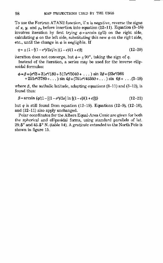
98 MAP PROJECTIONS USED BY THE USGS
To use the Fortran ATAN2 function, if n is negative, reverse the signs of x, y. and Po before insertion into equation (12-11). Equation (3-16) involves iteration by first trying <!>=arcsin (q/2) on the right side, calculating <f> on the left side, substituting this new <f> on the rig:tt side, etc., until the change in <f> is negligible. If
q = ± { 1-[(1- e2)/2e] ln [(1- e)/(1 + e)]J (12-20)
iteration does not converge, but <f> = ± 90°, taking the sign of q. Instead of the iteration, a series may be used for the invers8 ellip
soidal formulas:
<f>=fj+(e2/3+31e4/180+517e6/5040+ ... ) sin 2{j+(23e4/360 + 251e6/3780+ ... ) sin 4fj+(761~/45360+ ... ) sin 6/j+ ... (3-18)
where {j, the authalic latitude, adapting equations (3-11) and (3-12), is found thus:
{j =arcsin (q/(1- [(1- e2)/2e] ln [(1- e)/(1 +e)]}) (12-21)
but q is still found from equation (12-19). Equations (12-9), (12-10), and (12-11) also apply unchanged.
Polar coordinates for the Albers Equal-Area Conic are given for both the spherical and ellipsoidal forms, using standard parallels of lat. 29.5° ai).d 45.5° N. (table 14). A graticule extended to the North Pole is shown in figure 15.
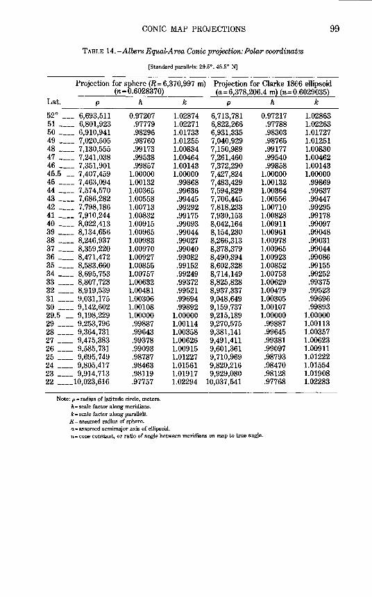
CONIC MAP PROJECTIONS 99
TABLE 14. -Albers Equal-Area Conic projection: Polar coordinat3s
[Standard parallels: 29.5°, 45.5° N]
Projection for sphere (R= 6,370,997 m) Projection for Clarke 1866 ellipsoid (n= 0.6028370) {a=6,378,206.4 m} {n=0.6029035}
Lat. p h k p h k
52° --- 6,693,511 0.97207 1.02874 6,713,781 0.97217 1.02863 51 ---- 6,801,923 .97779 1.02271 6,822,266 .97788 1.02263 50 ---- 6,910,941 .98296 1.01733 6,931,335 .98303 1.01727 49 ---- 7,020,505 .98760 1.01255 7,040,929 .98765 1.01251 48 ---- 7,130,555 .99173 1.00834 7,150,989 .99177 1.00830 47 ---- 7,241,038 .99538 1.00464 7,261,460 .99540 1.00462 46 ---- 7,351,901 .99857 1.00143 7,372,290 .99858 1.00143 45.5 -- 7,407,459 1.00000 1.00000 7,427,824 1.00000 1.00000 45 ---- 7,463,094 1.00132 .99868 7,483,429 1.00132 .99869 44 ---- 7,574,570 1.00365 .99636 7,594,829 1.00364 .99637 43 ---- 7,686,282 1.00558 .99445 7,706,445 1.00556 .99447 42 ---- 7' 798' 186 1.00713 .99292 7,818,233 1.00710 .99295 41 ---- 7,910,244 1.00832 .99175 7,930,153 1.00828 .99178 40 ---- 8,022,413 1.00915 .99093 8,042,164 1.00911 .99097 39 ---- 8,134,656 1.00965 .99044 8,154,230 1.00961 .99048 38 ---- 8,246,937 1.00983 .99027 8,266,313 1.00978 .99031 37 ---- 8,359,220 1.00970 .99040 8,378,379 1.00965 .99044 36 ---- 8,471,472 1.00927 .99082 8,490,394 1.00923 .99086 35 ---- 8,583,660 1.00855 .99152 8,602,328 1.00852 .99155 34 ---- 8,695,753 1.00757 .99249 8,714,149 1.00753 .99252 33 ---- 8,807 '723 1.00632 .99372 8,825,828 1.00629 .99375 32 ---- 8,919,539 1.00481 .99521 8,937,337 1.00479 .99523 31 ---- 9,031,175 1.00306 .99694 9,048,649 1.00305 .99696 30 ---- 9,142,602 1.00108 .99892 9,159,737 1.00107 .99893 29.5 -- 9,198,229 1.00000 1.00000 9,215,189 1.00000 1.00000 29 ---- 9,253,796 .99887 1.00114 9,270,575 .99887 1.00113 28 ---- 9,364,731 .99643 1.00358 9,381,141 .99645 1.00357 27 ---- 9,475,383 .99378 1.00626 9,491,411 .99381 1.00623 26 ---- 9,585, 731 .99093 1.00915 9,601,361 .99097 1.00911 25 ---- 9,695,749 .98787 1.01227 9,710,969 .98793 1.01222 24 ---- 9,805,417 .98463 1.01561 9,820,216 .98470 1.01554 23 ---- 9,914, 713 .98119 1.01917 9,929,080 .98128 1.01908 22 ____ 10,023,616 .97757 1.02294 10,037,541 .97768 1.02283
Note: p =radius of latitude circle, meters. h= scale factor along meridians. k =scale factor along parallels. R =assumed radius of sphere. a= assumed semimajor axis of ellipsoid. n= cone constant, or ratio of angle between meridians on map to true angle.

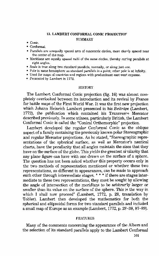
13. LAMBERT CONFORMAL CONIC PROJECTIOl'T
SUMMARY • Conic. • Conformal. • Parallels are unequally spaced arcs of concentric circles, more cloEP.ly spaced near
the center of the map. • Meridians are equally spaced radii of the same circles, thereby cut~ing parallels at
right angles. • Scale is true along two standard parallels, normally, or along just one. • Pole in same hemisphere as standard parallels is a point; other pok is at infinity. • Used for maps of countries and regions with predominant east-west, expanse. • Presented by Lambert in 1772.
HISTORY
The Lambert Conformal Conic projection (fig. 16) was almost completely overlooked between its introduction and its revival by France for battle maps of the First World War. It was the first new projection which Johann Heinrich Lambert presented in his Beitrii{te (Lambert, 1772), the publication which contained his Transverf~ Mercator described previously. In some atlases, particularly British, the Lambert Conformal Conic is called the "Conical Orthomorphic" projection.
Lambert developed the regular Conformal Conic as the oblique aspect of a family containing the previously known polar Stereographic and regular Mercator projections. As he stated, "Stereographic representations of the spherical surface, as well as Mercator's nautical charts, have the peculiarity that all angles maintain the sizes that they have on the surface of the globe. This yields the greatest si'llilarity that any plane figure can have with one drawn on the surface of a sphere. The question has not been asked whether this property occurs only in the two methods of representation mentioned or whether these two representations, so different in appearances, can be made to approach each other through intermediate stages. * * * if there are stages intermediate to these two representations, they must be sought by allowing the angle of intersection of the meridians to be arbitrarly larger or smaller than its value on the surface of the sphere. This is the way in which I shall now proceed" (Lambert, 1772, p. 28, translation by Tobler). Lambert then developed the mathematics for both the spherical and ellipsoidal forms for two standard parallels and included a small map of Europe as an example (Lambert, 1772, p. 28-38, 87-89).
FEATURES
Many of the comments concerning the appearance of the Albers and the selection of its standard parallels apply to the Lambert Conformal
101
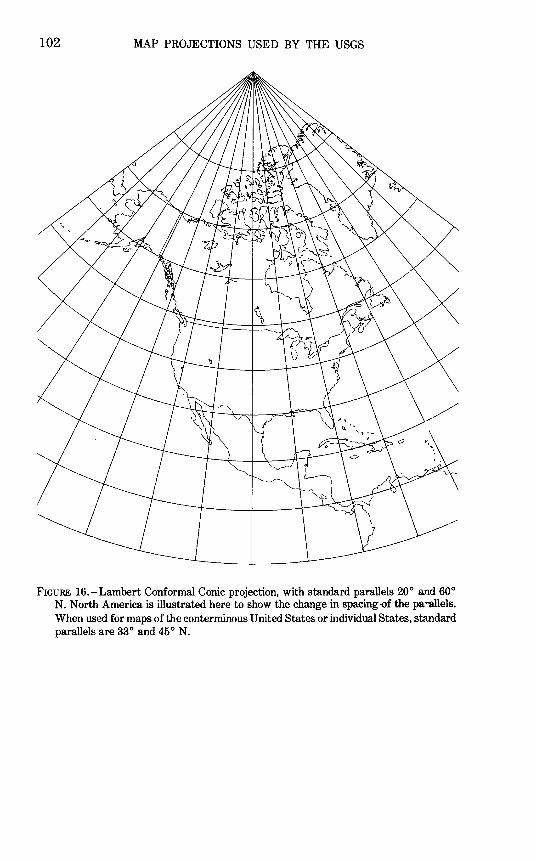
102 MAP PROJECTIONS USED BY THE USGS
FIGURE 16.-Lambert Conformal Conic projection, with standard parallels 20° and 60° N. North America is illustrated here to show the change in spacing-of the pa"'allels. When used for maps of the conterminous United States or individual States, standard parallels are 33° and 45° N.
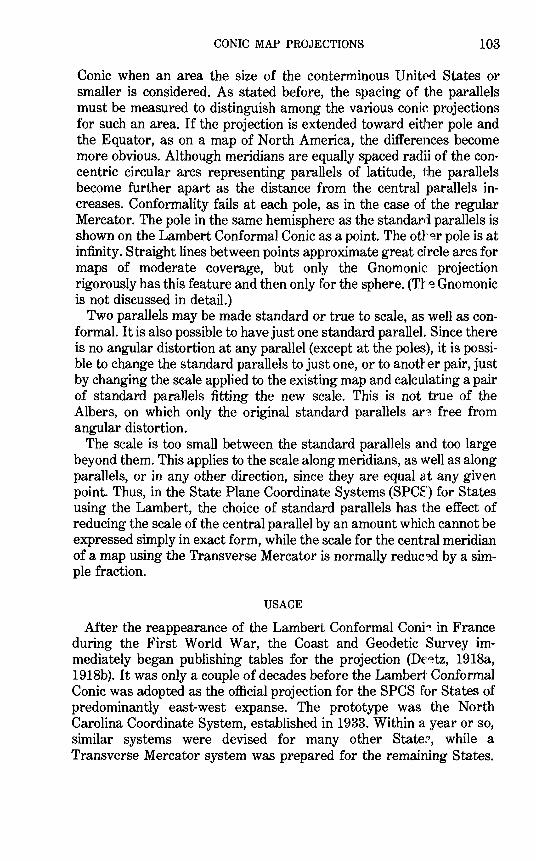
CONIC MAP PROJECTIONS 103
Conic when an area the size of the conterminous UnitM States or smaller is considered. As stated before, the spacing of the parallels must be measured to distinguish among the various conic projections for such an area. If the projection is extended toward either pole and the Equator, as on a map of North America, the differences become more obvious. Although meridians are equally spaced radii of the concentric circular arcs representing parallels of latitude, the parallels become further apart as the distance from the central parallels increases. Conformality fails at each pole, as in the case of the regular Mercator. The pole in the same hemisphere as the standard parallels is shown on the Lambert Conformal Conic as a point. The ot}'o.r pole is at infinity. Straight lines between points approximate great circle arcs for maps of moderate coverage, but only the Gnomonic projection rigorously has this feature and then only for the sphere. (Tr~ Gnomonic is not discussed in detail.)
Two parallels may be made standard or true to scale, as well as conformal. It is also possible to have just one standard parallel. Since there is no angular distortion at any parallel (except at the poles), it is possible to change the standard parallels to just one, or to another pair, just by changing the scale applied to the existing map and calculating a pair of standard parallels fitting the new scale. This is not true of the Albers, on which only the original standard parallels ar~ free from angular distortion.
The scale is too small between the standard parallels and too large beyond them. This applies to the scale along meridians, as well as along parallels, or in any other direction, since they are equal at any given point. Thus, in the State Plane Coordinate Systems (SPCt') for States using the Lambert, the choice of standard parallels has the effect of reducing the scale of the central parallel by an amount whieh cannot be expressed simply in exact form, while the scale for the central meridian of a map using the Transverse Mercator is normally reduc~~d by a simple fraction.
USAGE
After the reappearance of the Lambert Conformal Coni~ in France during the First World War, the Coast and Geodetic Survey immediately began publishing tables for the projection (De~tz, 1918a, 1918b). It was only a couple of decades before the Lambert Conformal Conic was adopted as the official projection for the SPCS for States of predominantly east-west expanse. The prototype was the North Carolina Coordinate System, established in 1933. Within a year or so, similar systems were devised for many other State;;-, while a Transverse Mercator system was prepared for the remaining States.
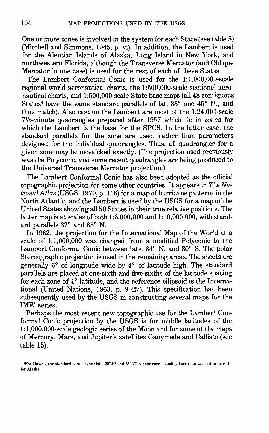
104 MAP PROJECTIONS USED BY THE USGS
One or more zones is involved in the system for each State (see table 8) (Mitchell and Simmons, 1945, p. vi). In addition, the Lambert is used for the Aleutian Islands of Alaska, Long Island in New York, and northwestern Florida, although the Transverse Mercator (and Oblique Mercator in one case) is used for the rest of each of these Stat~~s.
The Lambert Conformal Conic is used for the 1:1,000,001-scale regional world aeronautical charts, the 1:500,000-scale sectional aeronautical charts, and 1:500,000-scale State base maps (all48 contiguous States4 have the same standard parallels of lat. 33° and 45° ~T., and thus match). Also cast on the Lambert are most of the 1:24,001-scale 71fz-minute quadrangles prepared after 1957 which lie in zor~s for which the Lambert is the base for the SPCS. In the latter case, the standard parallels for the zone are used, rather than para1neters designed for the individual quadrangles. Thus, all quadrangler for a given zone may be mosaicked exactly. (The projection used pre,.riously was the Polyconic, and some recent quadrangles are being produced to the Universal Transverse Mercator projection.)
The Lambert Conformal Conic has also been adopted as the official topographic projection for some other countries. It appears in T';,e National Atlas (USGS, 1970, p. 116) for a map of hurricane pattern~ in the North Atlantic, and the Lambert is used by the USGS for a map of the United States showing all 50 States in their true relative positiors. The latter map is at scales of both 1:6,000,000 and 1:10,000,000, with standard parallels 37° and 65° N.
In 1962, the projection for the International Map of the Wor~d at a scale of 1:1,000,000 was changed from a modified Polyconic to the Lambert Conformal Conic between lats. 84° N. and 80° S. The polar Stereographic projection is used in the remaining areas. The sheets are generally 6° of longitude wide by 4° of latitude high. The st2ndard parallels are placed at one-sixth and five-sixths of the latitude spacing for each zone of 4 o latitude, and the reference ellipsoid is the International (United Nations, 1963, p. 9-27). This specification haf been subsequently used by the USGS in constructing several maps for the IMW series.
Perhaps the most recent new topographic use for the Lamber+. Conformal Conic projection by the USGS is for middle latitudes of the 1:1,000,000-scale geologic series of the Moon and for some of the maps of Mercury, Mars, and Jupiter's satellites Ganymede and Callisto (see table 15).
•For Hawaii, the standard parallels are lats. 20°40' and 23°20' N.; the corresponding base map was not prepared for Alaska.
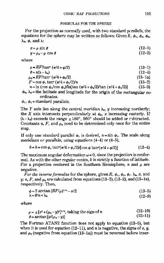
CONIC MAP PROJECTIONS 105
FORMULAS FOR THE SPHERE
For the projection as normally used, with two standard pr.rallels, the equations for the sphere may be written as follows: Given R, cf>h c/>z, c/>o, Ao, c/>, and A:
X= p sin() Y= po-p cos()
where
(12-1) (12-2)
p=RF/tan" (rl4+ct>l2) (13-1) 8=n(A-Ao) (12-4)
p0 =RF/tan" (r/4+cf>0/2) (13-1a) F =cos c/>1 tan" ( r/4 + c/>1/2)/n (13-2) n=In (cos c/>1/cos c/>1)/ln[tan (r/4+cl>z/2)/tan (r/4+cf>1/2)] (13-3)
cl>o, Ao =the latitude and longitude for the origin of the rectangular co-ordinates.
c/>11 c/>z =standard parallels.
The Y axis lies along the central meridian Ao, y increasing northerly; the X axis intersects perpendicularly at cp0 , x increasing easterly. If (A- Ao) exceeds the range ± 180°, 360° should be added or rnbtracted. Constants n, F, and p0 need to be determined only once for the entire map.
If only one standard parallel c/>1 is desired, n = sin c/l1. The scale along meridians or parallels, using equations ( 4-4) or ( 4-5),
k= h= cos c/>1 tan"(r/4+ c/>1/2)/[ cos q, tan"(r/4 + cf>/2)] (13-4)
The maximum angular deformation w = 0, since the projectio'l is conformal. As with the other regular conics, k is strictly a function of latitude. For a projection centered in the Southern Hemisphere, n and p are negative.
For the inverse formulas for the sphere, given R, c/l11 c/>z, cf>c, Ao, x, and y: n, F, and Po are calculated from equations (13-3), (13-2), and (13-1a), respectively. Then,
cp = 2 arctan (RF/ p )1'"- 1r/2
A=81n+Ao
where
p = ± [x2 +(p0 -y)2]
112, taking the sign of n
()=arctan [ xl(po- y)]
(13-5) (12-9)
(12-10) (12-11)
The Fortran ATAN2 function does not apply to equation (13-5), but when it is used for equation (12-11), and n is negative, the signs of x, y, and Po (negative from equation (13-1a)) must be reversed before inser-
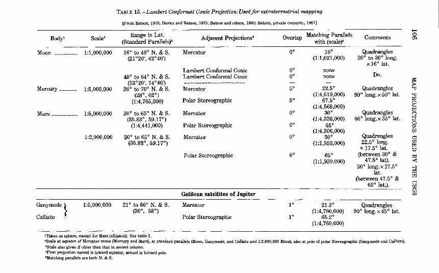
TABLE 15.-Lambert Conformal Conic Projection:Usedfor extraterrestrial mapping
[From Batson, 1973; Davies and Batson, 1975; Batson and others, 1980; Batson, private commun., 1981]
Body' Scale1 Range in Lat. Adjacent Projections4 Overlap Matching Parallels Comments (Standard Parallels)3 with (scale)5
Moon -------- 1:1,000,000 16° to 48° N. & S. Mercator oo 16° Quadrangles (21 °20', 42°40') (1:1,021,000) 20° to 30° long.
x 16° lat. Lambert Conformal Conic oo none
48° to 64° N. & S. Lambert Conformal Conic oo none Do. (53°20', 74°40') ---------------------
Mercury ______ 1:5,000,000 20° to 70° N. & S. Mercator 50 22.5° Quadrangles (28°, 62°) (1:4,619,000) 90° long. x 50° lat.
(1:4, 765,000) Polar Stereographic 50 67.5° (1:4,568,000)
Mars --------- 1:5,000,000 30° to 65° N. & S. Mercator oo 30° Quadrangles (35.83°' 59.17°) (1 :4,336,000) 60° long. x 35° lat.
(1:4,441,000) Polar Stereographic oo 65° (1:4,306,000)
Quadrangles 1:2,000,000 30° to 65° N. & S. Mercator oo 30° (35.83°' 59.17°) (1:1,953,000) 22.5° lo~g.
x 17.5° lat. Polar Stereographic oo 65° (between 30° &
(1:1,939,000) 47.5° lat). 30° long.x 17.5°
lat. (between 4 7.5 o &
65° lat.).
Galilean satellites of Jupiter
Ganymede} 1:5,000,000 21° to 66° N. & S. Mercator 10 21.3° Quadrangles (30°, 58°) (1 :4, 780,000) 90° long. x 45 o lat.
Callisto , Polar Stereographic 10 65.2° (1:4, 769,000)
1Taken as sphere, except for Mars (ellipsoid). See table 2. 2Scale at equator of Mercator zones (Mercury and Mars), at standard parallels (Moon, Ganymede, and Callisto and 1:2,000,000 Mars), also at pole of polar Stereographic (Ganymede and Callisto). •scale also given if other than that in second column. •First projection named is toward equator, second is toward pole. •Matching parallels are both N. & S.
~ 0 m
s= > "'0
"'0
~ <:...; t?:l 0 t-3
~ 'C/).
c::: 'C/).
t?:l t::l t:l:l t-< t-3 ::c: t%j
c::: 'C/).
4.l 'C/).
CONIC MAP PROJECTIONS 107
tion into the equation. If p = 0, equation (13-5) involves division by zero, but <P is ± 90°, taking the sign of n.
The standard parallels normally used for maps of the corterminous United States are lats. 33 o and 45 ° N., which give approxi:-nately the least overall error within those boundaries. The ellipsoidal fr~m is used for such maps, based on the Clarke 1866 ellipsoid (Adams, 1918).
The standard parallels of 33° and 45° were selected by the USGS because of the existing tables by Adams (1918), but Adams chose them to provide a maximum scale error between latitudes 30.5° and 47.5° of one-half of 1 percent. A maximum scale error of 2.5 percent occurs in southernmost Florida (Deetz and Adams, 1934, p. 80). Othe':' standard parallels would reduce the maximum scale error for the United States, but at the expense of accuracy in the center of the map.
FORMULAS FOR THE ELLIPSOID
The ellipsoidal formulas are essential when applying the Lambert Conformal Conic to mapping at a scale of 1:100,000 or larger and important at scales of 1:5,000,000. Given a, e, <Ph </>1, cf>o, Ao, cp, and A:
where
X= p sin() Y = Po- p COS 8 k= pnl(am)
= m,tnf(mt,n)
p=aFtn 8=n(A-Ao)
p0 =aFton n = (ln m1 -In m1)/(ln t, -In tz)
m= cos cp/(1- e1 sin1 cp)111
t =tan ( 1rl4- cp/2)/[(1- e sin cp )/(1 + e sin cp )]en F=m,l(nt1n)
(12-1) (12-2)
(12-16) (13-6)
(13-7) (12-4)
(13-7a) (13-8)
(12-15) (13-9)
(13-10)
with the same subscripts 1, 2, or none applied tom and <Pin equation (12-15), and 0, 1, 2, or none applied to t and <P in equation (If -9), as required by equations (13-6), (13-7), and (13-8). As with othe~ conics, a negative n and p result for projections centered in the Southern Hemisphere. If cp = ± 90°, p is zero for the same sign as n and infinite for the opposite sign. If</>.= <Pz, for the Lambert with a single standard parallel, equation (13-8) is indeterminate, but n= sin ¢ •. C.'igin and orientation of axes for x and y are the same as those for the spherical form. Constants n, F, and Po may be determined just once for the entire map.
When the above equations for the ellipsoidal form are used~ they give values of n and p slightly different from those in the accepted tables of
108 MAP PROJECTIONS USED BY THE USGS
coordinates for a map of the United States, according to the Lambert Conformal Conic projection. The discrepancy is 35-50 m in th ~ radius and 0.0000035 inn. The rectangular coordinates are correspondingly affected. The discrepancy is less significant when·it is realized that the radius is measured to the pole, and that the distance from the 50th parallel to the 25th parallel on the map at full scale is only 12 m out of 2,800,000 or 0.0004 percent. For calculating convenience 60 ye~.rs ago, the tables were, in effect, calculated using instead of equation (13-9),
t = tan ( r/ 4- c/J,/2) (13-9a)
where c/J11 is the geocentric latitude, or, as shown earlier,
cP11 =arctan [(1- e2)tan c/J] (3-28)
In conventional terminology, the t of equation (13-9) is usually written as tan 1/2Z, where Z is the colatitude of the conformallatitud~ x (see equation (3-1)).
For the existing tables, then, c/J11 , the geocentric latitude, was used for convenience in place of x, the conformal latitude (Adams, 1918, p. 6-9, 34). A comparison of series equations (3-3) and (3-30), or of the corresponding columns in table 3, shows that the two al1xiliary latitudes x and c/J11 are numerically very nearly the same.
There may be much smaller discrepancies found between com-riinates as calculated on modern computers and those listed in tables for the SPCS. This is due to the slightly reduced (but sufficient) accuracv of the desk calculators of 30-40 years ago and the adaptation of formulas to be more easily utilized by them.
The inverse formulas for ellipsoidal coordinates, given a, e, c/J., c/J2, c/Jo, ~' c/J, and h: n, F, and Po are calculated from equations (13-8), (13-10), (13-7a), respectively. Then,
where
c/J= r/2- 2 arctan {t[(1- e sin c/J)/(1 + e sin c/J)]•12} (7-9)
t = (p/ aF)l!n
p = ± [x2 -(p0 - y)2]
112, taking the sign of n.
h=81n+A.o 8 =arctan [x/(p 0 - y)]
(13-11) (12-10) (12-9)
(12-11)
As with the spherical formulas, the Fortran ATAN2 function cl'les not apply to equation (7-9), but for equation (12-11), if n is negative, the signs of x, y, and p0 must be reversed.
Equation (7-9) involves rapidly converging iteration: Calculate t from (13-11). Then, assuming an initial trial c/J equal to (?r/2-2 arctan t) in the right side of equation (7-9), calculate cfJ on the le~t side. Substitute the calculated c/J into the right side, calculate a new</>, etc., until <P does not change significantly from the preceding trial value of c/J.
CONIC MAP PROJECTIONS 109
To avoid iteration, series (3-5) may be used with (7 -13) in place of (7-9):
<1> = x + ( e212 + 5e4/24 + e6/12 + ... ) sin 2x + (7 e-4/48 + 29e6/240 + ... ) sin 4x + (7e6/120 + ... ) sin 6x +. . . (3-5)
where
x = 1fl2- 2 arctan t (7-13)
If rectangular coordinates for maps based on the tables u~·1ng geocentric latitude are to be converted to latitude and longitude, the inverse formulas are the same as those above, except that equation (13-9a) is used instead of (13-9) for calculations leading to n, F, and p 0 , and equation (7 -9), or (3-5) and (7 -13), is replaced with the following~ which does not involve iteration:
cp = arctan [tan cfl/(1- e2)] (13-13)
where
cp, = 1fl2- 2 arctan t (13-14)
and t is calculated from equation (13-11). Polar coordinates for the Lambert Conformal Conic a:re given for
both the spherical and ellipsoidal forms, using standard parallels of 33° and 45° N. (table 16). The data based on the geocentric latitude are given for comparison. A graticule extended to the North Pole is shown in figure 16.

14. BIPOLAR OBLIQUE CONIC CONFORMAL PROJECTION
SUMMARY
• Two oblique conic projections, side-by-side, but with poles 104 o apart. • Conformal. • Meridians and parallels are complex curves, intersecting at right angles. • Scale is true along two standard transformed parallels on each conic projection,
neither of these lines following any geographical meridian or paralle1•
• Very small deviation from conformality, where the two conic projecticns join. • Specially developed for a map of the Americas. • Used only in spherical form. • Presented by Miller and Briesemeister in 1941.
HISTORY
A "tailor-made" projection is one designed for a certain geographical area. 0. M. Miller used the term for some projections which he developed for the American Geographical Society (AGS) or for their clients. The Bipolar Oblique Conic Conformal projection, developed with William A. Briesemeister, was presented in 1941 and designed specifically for a map of North and South America con~tructed in several sheets by the AGS at a scale of 1:5,000,000 (Miller, 1941).
It is an adaptation of the Lambert Conformal Conic projection to minimize scale error over the two continents by accommoiating the fact that North America tends to curve toward the east as on~ proceeds from north to south, while South America tends to curve in the opposite direction. Because of the relatively small scale of th~ map, the Earth was treated as a sphere. To construct the map, a great circle arc 104 ° long was selected to cut through Central America from southwest to northeast, beginning at lat. 20° S. and long. 110° W. and terminating at lat. 45° N. and the resulting longitude of about 19°59'36" w.
The former point is used as the pole and as the center of tr-:~.nsformed parallels of latitude for an Oblique Conformal Conic proj€.ction with two standard parallels (at polar distances of 31 o and 73°) for all the land in the Americas southeast of the 104 o great circle arc. The latter point serves as the pole and center of parallels for an identical projection for all land northwest of the same arc. The inner and outer standard parallels of the northwest portion of the map, thus, are tangent to the outer and inner standard parallels, respectively, of the southeast portion, touching at the dividing line (104 o- 31 o = 73°).
111
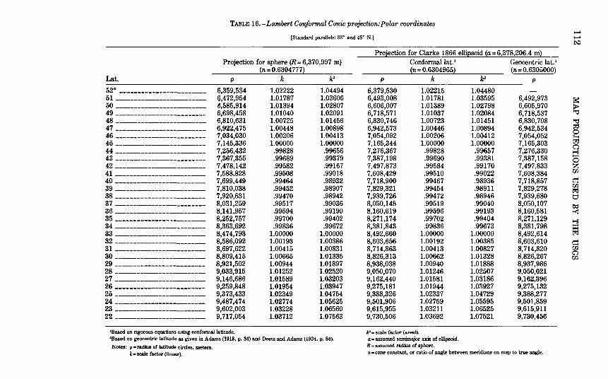
TABLE 16.-Lambert Conformal Conic projection:Polar coordinates ~
[Standard parallels: 33• and 45° N.) ~ ~
Projection for Clarke 1866 elliEsoid {a=6,378,206.4 m} Projection for sphere (R = 6,370,997 m) Conformal lat. 1 Geocentric lat.1
{n=0.6304777} {n = 0.6304965} (n= 0.6305000) Lat. p k k1 p k k1 p
52° ------------------------ 6,359,534 1.02222 1.04494 6,379,530 1.02215 1.04480 51 ------------------------- 6,472,954 1.01787 1.03606 6,493,008 1.01781 1.03595 6,492,973 a:: 50 ------------------------- ~.585,914 1.01394 1.02807 6,606,007 1.01389 1.02798 6,605,970 > 49 _________________________
6,698,458 1.01040 1.02091 6,718,571 1.01037 1.02084 6,718,537 """0
48 ------------------------- 6,810,631 1.00725 1.01456 6,830,746 1.00723 1.01451 6,830,708 ~
47 ------------------------- 6,922,475 1.00448 1.00898 6,942,573 1.00446 1.00894 6,942,534 ~ 0 46 _________________________
7,034,030 1.00206 1.00413 7,054,092 1.00206 1.00412 7,054,052 ~
45 ------------------------- 7,145,336 1.00000 1.00000 7,165,344 1.00000 1.00000 7,165,303 tr.l 0
44 ------------------------- 7,256,432 .99828 .99656 7,276,367 .99828 .99657 7,276,330 1-3
43 ------------------------- 7,367,355 .99689 .99379 7,387,198 .99690 .99381 7,387,158 -0 42 ------------------------- 7,478,142 .99582 .99167 7,497,873 .99584 .99170 7,497,833 z 41 ------------------------- 7,588,828 .99508 .99018 7,608,429 .99510 .99022 7,608,384 w
40 ------------------------- 7,699,449 .99464 .98932 7,718,900 .99467 .98936 7,718,857 c::: 39 ------------------------- 7,810,038 .99452 .98907 7,829,321 .99454 .98911 7,829,278 w
tr.l 38 _________________________ 7,920,631 .99470 .98942 7,939,726 .99472 .98946 7,939,680 t::l
37 ------------------------- 8,031,259 .99517 .99036 8,050,148 .99519 .99040 8,050,107 ~ 36 ------------------------- 8,141,957 .99594 .99190 8,160,619 .99596 .99193 8,160,581
35 ------------------------- 8,252,757 .99700 .99402 8,271,174 .9970.2 .99404 8,271,129 1-3 34 ------------------------- 8,363,692 .99836 .99672 8,381,843 .99836 .99673 8,381,798 t:I:: 33 ------------------------- 8,474,793 1.00000 1.00000 8,492,660 1.00000 1.00000 8,492,614 tr.l
32 ------------------------- 8,586,092 1.00193 1.00386 8,603,656 1.00192 1.00385 8,603,610 c::: 31 ------------------------- 8,697,622 1.00415 1.00831 8,714,863 1.00413 1.00827 8,714,820 w 30 _________________________
8,809,415 1.00665 1.01335 8,826,313 1.00662 1.01328 8,826,267 C".:l w 29 ------------------------- 8,921,502 1.00944 1.01897 8,938,038 1.00940 1.01888 8,937,986
28 ------------------------- 9,033,915 1.01252 1.02520 9,050,070 1.01246 1.02507 9,050,021
27 ------------------------- 9,146,686 1.01589 1.03203 9,162,440 1.01581 1.03186 9,162,396 26 _________________________ 9,259,848 1.01954 1.03947 9,275,181 1.01944 1.03927 9,275,132
25 ------------------------- 9,373,433 1.02349 1.04754 9,388,326 1.02337 1.04729 9,388,277
24 ------------------------- 9,487,474 1.02774 1.05625 9,501,906 1.02759 1.05595 9,501,859
23 ------------------------- 9,602,003 1.03228 1.06560 9,615,955 1.03211 1.06525 9,615,911
22 ------------------------- 9,717,054 1.03712 1.07563 9,730,506 1.03692 1.07521 9,730,456
'Based on rigorous equations using conformal latitude. k' =scale factor (areal). 'Based on geocentric latitude as given in Adams (1918, p. 34) and Deetz and Adams (1934, p. 84). a-assumed semimajor axis of ellipsoid.
Notes: p • radius of latitude circles, meters. R-assumed radius of sphere.
k·scale factor (linear). n- cone constant, or ratio of angle between meridians on map to true angle.
CONIC MAP PROJECTIONS 113
The scale of the map was then increased by about 3.5 percent, so that the linear scale error along the central parallels (at a polar distance of 52°, halfway between 31 o and 73°) is equal and opposite in sign (- 3.5 percent) to the scale error along the two standard parallels (now + 3.5 percent) which are at the normal map limits. Under these conditions, transformed parallels at polar distances of about 36.34 o and 66.58° are true to scale and are actually the standard transformed parallels.
The use of the Oblique Conformal Conic projection was n':lt original with 1\iiller and Briesemeister. The concept involves the shifting of the graticule of meridians and parallels for the regular Lambert Conformal Conic so that the pole of the projection is no longer at the pole of the Earth. This is the same principle as the transformation for the Oblique Mercator projection. The bipolar concept is unique, however, and it has apparently not been used for any other maps.
FEATURES AND USAGE
The Geological Survey has used the North American po~.ion of the map for the Geologic Map (1965), the Basement Map (1967), the Geothermal Map, and the Metallogenic Map, all retaining the original scale of 1:5,000,000. The Tectonic Map of North America (1969) is generally based on the Bipolar Oblique Conic Conformal, but there are modifications near the edges. An oblique conic projection abcut a single transformed pole would suffice for either one of the continents alone, but the AGS map served as an available base map at an appropriate scale. In 1979, the USGS decided to replace this projectio:"l with the Transverse Mercator for a map of North America.
The projection is conformal, and each of the two conic projections has all the characteristics of the Lambert Conformal Conic proj~ction, except for the important difference in location of the pole, and a very narrow band near the center. While meridians and parallels on the oblique projection intersect at right angles because the map is conformal, the parallels are not arcs of circles, and the meridians are not straight, except for the peripheral meridian from each transformed role to the nearest normal pole.
The scale is constant along each circular arc centered on the transformed pole for the conic projection of the particular portion of the map. Thus, the two lines at a scale factor of 1.035, th~.t is, both pairs of the official standard transformed parallels, are map"led as circular arcs forming the letter "S." The 104 o great circle arc separating the two oblique conic projections is a straight line on the map, and all other straight lines radiating from the poles for the respective conic projections are transformed meridians and are therefore great circle routes. These straight lines are not normally shown on tre finished map.
114 MAP PROJECTIONS USED BY THE USGS
At the juncture of the two conic projections, along the 104: o axis, there is actually a slight mathematical discontinuity at every p<:lint except for the two points at which the transformed parallels of polar distance 31 o and 73° meet. If the conic projections are strictly followed, there is a maximum discrepancy of 1.6 mm at the 1:5,000,000 scale at the midpoint of this axis, halfway between the poles or l'~tween the intersections of the axis with the 31 o and 73° tram·formed parallels. In other words, a meridian approaching the axis fr0m the south is shifted up to 1. 6 mm along the axis as it crosses. Al')ng the axis, but beyond the portion between the lines of true scale, the discrepancy increases markedly, until it is over 240 mm at the transformed poles. These latter areas are beyond the needed range of the map and are not shown, just as the polar areas of the regular Lambert Conformal Conic are normally omitted. This would r0t happen if the Oblique Equidistant Conic projection were used.
The discontinuity was resolved by connecting the two arcs with a straight line tangent to both, a convenience which leaves the small intermediate area slightly nonconformal. This adjustment is inchded in the formulas below.
FORMULAS FOR THE SPHERE
The original map was prepared by the American Geographical Society, in an era when automatic plotters and easy computation of coordinates were not yet present. Map coordinates were determined by converting the geographical coordinates of a given graticule inter()ection to the transformed latitude and longitude based on the poles of the projection, then to polar coordinates according to the conformal projection, and finally to rectangular coordinates relative to the ~·elected origin.
The following formulas combine these steps in a form which may be programed for the computer. First, various constants are cahulated from the above parameters, applying to the entire map. Since only one map is involved, the numerical values are inserted in formulas, except where the numbers are transcendental and are referred to by s~rmbols.
If the southwest pole is at point A, the northeast pole is at r0int B, and the center point on the axis is C,
AB= -110° +arccos ([cos 104°- sin ( -20°) sin 45°]/ [cos (- 20°) cos 45°]) (14-1)
= -19°59'36" long., the longitude of B (negative is west long.) n= (In sin 31 o -In sin 73°)/[ln tan (31 o /2)-ln tan (73° /2)] (14-2)
= 0.63056, the cone constant for both conic projections
CONIC MAP PROJECTIONS 115
F 0 =R sin 31 °/[n tan" (31 °/2)] (14-3) = 1.83376 R, where R is the radius of the globe at the scale of the
map. For the 1:5,000,000 map, R was taken as 6,371,221 m, the radius of a sphere having a volume equal to that of the International ellipsoid.
ko=2/[1+nF0 tan" 26°/(R sin 52°)] (14-4) = 1.03462, the scale factor by which the coordinates are multiplied
to balance the errors F=k0 F 0 (14-5)
= 1.89725 R, a convenient constant AzAs=arccos {[cos (-20°) sin 45°-sin (-20°) cos 45° cos
(As+ 110°)]/sin 104 °} (14-6) = 46.78203°, the azimuth east of north of B from A
AzsA=arccos ([cos 45° sin (-20°)-sin 45° cos (-20°) cos (As+ 110°)]/sin 104 °} (14-7)
= 104.42834 o, the azimuth west of north of A from B T =tan" (31 ° /2) +tan" (73° /2) (14-8)
= 1.27247, a convenient constant Pc= 112FT (14-9)
= 1.20709 R, the radius of the center point of the axis from either pole
Zc = 2 arctan (T/2)11" (14-10) = 52.03888°, the polar distance of the center point from either
pole
Note that zc would be exactly 52°, if there were no discontinuity at the axis. The values of cl>c, Ac, and Azc are calculated as if no adjustment were made at the axis due to the discontinuity. Their use is completely arbitrary and only affects positions of the arbitrary X and Y axes, not the map itself. The adjustment is included in formulas for a given point.
cl>c= arcsin [sin (- 20°) cos Zc+ cos (- 20°) sin Zc cosAzAB] (14-11) = 17°16'28" N. lat., the latitude of the center point, on the
southern-cone side of the axis Ac= arcsin (sin Zc sinAzAslcos cJ>c}-110° (14-12)
= -73°00'27" long., the longitude of the center point, on the southern-cone side of the axis
Azc= arcsin [cos (- 20°) sinAzAslcos cl>c] (14-13) = 45.81997°, the azimuth east of north of the axis at the center
point, relative to meridian Ac on the southern-cone side of the axis
The remaining equations are given in the order used, for calculating rectangular coordinates for various values of latitude cJ> and longitude A (measured east from Greenwich, or with a minus sign for the western values used here). It must be established first whether po~nt (c/>, A) is
116 MAP PROJECTIONS USED BY THE USGS
north or south of the axis, to determine which conic projection is involved. With these formulas, it is done by comparing the azi1mth of point (q,, A) with the azimuth of the axis, all as viewed from B:
Zs =arccos [sin 45 ° sin cP +cos 45 ° cos cP cos (As- A)] =polar distance of (cf>, A) from pole B
Azs =arctan {sin (As- A)/[ cos 45 ° tan cP- sin 45 ° cos (As- A)]l =azimuth of (q,, A) west of north, viewed from B
(14-14)
(14-15)
If Azs is greater than AzsA (from equation (14-7)), go to equation (14-23). Otherwise proceed to equation (14-16) for the projection from pole B.
ps=Ftann1f2Zs (14-16) k= psni(R sin Zs) (14-17)
=scale factor at point (cJ>, A), disregarding small adjustme:'lt near axis
a= arccos {[tann1f2zs + tann1f2(104 °- Zs)]IT} (14-18)
If In (AzsA -Azs)l is less than a,
ps' = Pslcos [a-n(AzsA -Azs)] (14-19)
If the above expression is equal to or greater than a,
I Ps = Ps· (14-20)
Then
x' = ps' sin [n (AzsA -Azs)] (14-21) y' = ps' cos [n (AzsA -Azs)]- p., (14-22)
using constants from equations (14-2), (14-3), (14-7), and (14-9) for rectangular coordinates relative to the axis. To change to nonskewed rectangular coordinates, go to equations (14-32) and (14-33). The following formulas give coordinates for the projection from p')le A.
ZA =arccos [sin (- 20°) sin cP +cos (- 20°) cos cP cos (A+ 110°)] (14-23) =polar distance of (cf>, A) from pole A
AzA =arctan {sin (A+ 110°)/[cos (- 20°) tan cf>- sin (- 20°) cos (A+ 110°)]} (14-24)
=azimuth of (cJ>, A) east of north, viewed from A PA =Ftann1f2zA k= pAn/R sin zA =scale factor at point (cf>, A) a= arccos ([tann1f2zA + tann1f2(104 °- zA)]IT}
If In (AzAB-AzA)I is less than a,
PA' = pA/cos [a+ n (AzAs- AzA)]
(14-25) (14-26) (14-27)
(14-28)
CONIC MAP PROJECTIONS 117
If the above expression is equal to or greater than a,
(14-29)
Then
x' = pA' sin [n(AzAs-AzA)J (14-30) y' =- pA' cos [n (AzAs-AzA)]+ p., (14-31) X= -x' cosAzc-Y sinAzc (14-32) Y= -y' cosAzc+x' sinAzc (14-33)
where the center point at (<Pc, A.,) is approximately the origi, of (x, y) coordinates, the Y axis increasing due north and the X axif due east from the origin. (The meridian and parallel actually crossing the origin are shifted by about 3' of arc, due to the adjustment at the axis, but their actual values do not affect the calculations here.)
For the inverse formulas for the Bipolar Oblique Conic Conformal, the constants for the map must first be calculated from equations (14-1}-(14-13). Given x and y coordinates based on the ab':lve axes, they are then converted to the skew coordinates:
x'= -xcosAzc+Y sinAzc (14-34) ?/= -xsinAzc-ycosAzc (14-35)
If x' is equal to or greater than zero, go to equation (14-36). If x' is negative, go to equation (14-45).
Ps' = [x'2 + (pc + y')l)112 Azs' =arctan [x'/(pc +y'))
Let
(14-36) (14-37)
Ps = Ps1 (14-38) Z8 = 2 arctan (p8 /F) 11
" (14-39) a=arccos ([tannlf2Z8 +tan"1/2(104° -z8 )]/T} (14-40)
If IAzs'l is equal to or greater than a, go to equation (14-42). If IAzs'l is less than a, calculate
p8 = p8 ' COS (a-Azs 1 (14-41)
and use this value to recalculate equations (14-39), (14-40), and (14-41), repeating until Ps found in (14-41) changes by less than a predetermined convergence. Then,
Az8 =AZ8~ -Azs'ln
Using Azs and the final value of Z8 ,
<P =arcsin (sin 45 ° cos Zs +cos 45 ° sin Zs cosAzs) A= A8 -arctan (sinAzs/[cos 45°/tan Z8 - sin 45° cosAzs]J
(14-42)
(14-43) (14-44)
118 MAP PROJECTIONS USED BY THE USGS
The remaining equations are for the southern cone only (negative x'):
PA' = [ x'l + (pc _ y')2)1!2 Azl= arctan [x'/(pc-y')]
Let
(14-45) (14-46)
PA = PA1 (14-4 7) zA = 2 arctan (pAIF) 11n (14-48) a= arccos ([tannlf2ZA + tann1f2(104 °- zA)]/T} (14-49)
If IAzA'I is equal to or greater than a, go to equation (14-51). If IAzA'I is less than a, calculate
PA = pA' cos (a+AzA') (14-50)
and use this value to recalculate equations (14-48), (14-49), and (14-50), repeating until PA found in equation (14-50) change~ by less than a predetermined convergence. Then,
AzA =AzAB-AzA'In (14-51)
Using AzA and the final value of zA,
cJ>= arcsin [sin (- 20°) cos zA +cos 20° sin zA cosAzA] (14-52) A= arctan {sin AzAI[ cos (- 20°)/tan zA- sin (- 20°) cos AzA]} -110°
(14-53)
Equations (14-17) or (14-26) may be used for calculating k afte':' cJ> and A are determined.
A table of rectangular coordinates is given in table 17, based on a radius R of 1.0, while a graticule is shown in figure 17.
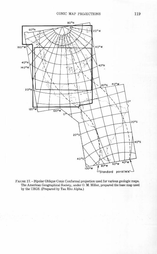
CONIC MAP PROJECTIONS 119
FIGURE 17. -Bipolar Oblique Conic Conformal projection used for various geologic maps. The American Geographical Society, under 0. M. Miller, prepared the base map used by the USGS. (Prepared by Tau Rho Alpha.)
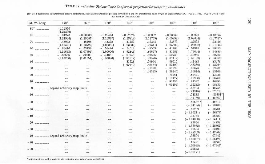
TABLE 17.-Bipolar Oblique Conic Conformal projection:Rectangular coordinates
[R = 1.0. y coordinates in parentheses below x coordinates. Solid line separates the portions formed from the two transformed poles. Origin at approximately lat. 17° 15' N ., long. 73°0~' W ., with Y axis due north at that point only]
Lat. W. Long.
90° --------
80 ---------
70 ---------
60 - --------
50 ----- ----
40 ---------
30 ---------
20 ---------
10 ---------
170°
- 0.14576 (1.24309)
- .31273 (1.21904)
- .48092 (1.19421)
- .65416 (1.16623)
- .83656 (1.13260)
160°
-0.30608 (1.19057)
- .46705 (1.13725)
- .63138 (1.07999)
- .80200 (1.01551)
0 _________ beyond arbitrary map limits
-10
- 20
- 30 ---------
-40
-50
- 60
- 70 _________ beyond arbitrary map limits
-80
- 90 ---------
150°
----
- 0.29464 (1.16367)
- .44372 (1.08381)
- .59444 (1.00006)
- .74851 ( .90886)
• Adjustment to x aild y made for discontinuity near axis .of conic projections.
140° 130°
- 0.27876 - 0.25892 (1.13914) (1.11769)
- .41182 - .37243 (1.03535) ( .99311)
- .54518 - .48559 ( .92849) ( .86677)
- .67943 - .59806 ( .81512) ( .73570)
- .81523 - .70964 ( .69140) ( .59654)
- .81990 ( .44545)
120°
-0.23569 (1.09992)
- .32673 ( .95806)
- .41763 ( .81589)
- .50739 ( .67112)
- .59515 ( .52100)
- .67999 ( .36240)
- .76061 ( .19177)
- .83496 ( .00499)
110°
-0.20973 (1.08634)
- .27593 ( .93098)
- .34310 ( .77644)
- .40985 ( .62133)
- .47485 ( .46360)
- .53678 ( .30074)
- .59421 ( .12988)
- .64522 (- .05222) - .68704 (- .24918) - .72338 (- .47150) - .86567 * (- .84124) - .55209
( - 1.10271) - .37784
( -1.24800) - .23054
( -1.37082) - .09524
( -1.48363) .03504
( - 1.59227) .16491
( - 1.70055) .29823
( -1.81171)
100°
-0.18175 (1.07737)
- .22126 ( .91246)
- .26359 ( .74880)
- .30732 ( .58603)
- .35078 ( .42294)
- .39231 ( .25766)
- .43026 ( .08782)
- .46280 (- .08930) - .48758 (- .27670) - .50751* (- .48360 - .48812 (-.73406) - .38781 (- .96476) - .26583
( -1.14111) - .14798
( -1.28862) - .03499
( -1.42268) .07542
( - 1.55124) .18569
( - 1.67949)
~ t...:l 0
s::: > "'0
"'0 ~ 0 ~ tzj 0 ~ ....... 0 z UJ
e UJ tzj t::1 t:l:l ~
~ ~ tzj
e UJ CJ UJ
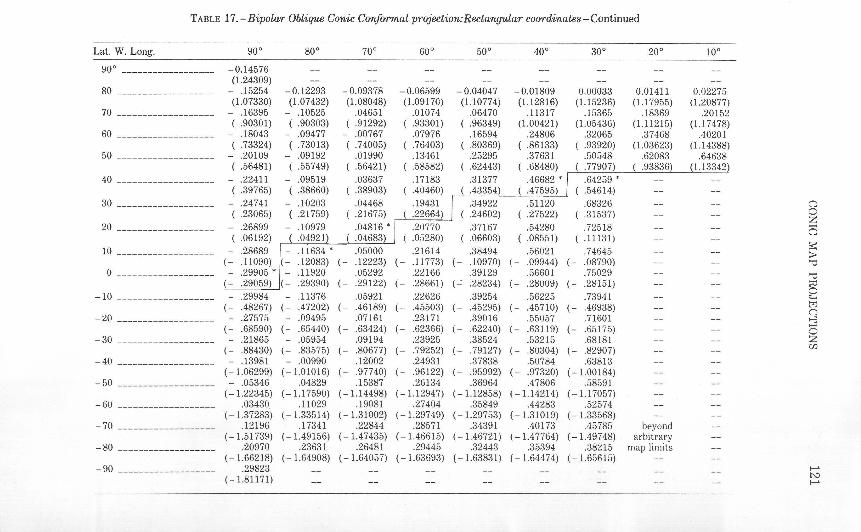
TABLE 17.-Bipolar Oblique Conic Conformal projection: Rectangular coordinates- Continued
Lat. W. Long. goo 80° 70° 60° 50° 40° 30° 20° 100
90° ------------------ -0.14576 (1.24309)
80 ------------------- - .15254 -0.12293 -0.09378 -0.06599 -0.04047 - 0.01809 0.00033 0.01411 0.02275 (1.07330) (1.07432) (1.08048) (1.09170) (1.10774) (1.12816) (1.15236) (1.17955) (1.20877)
70 ------------------- - .16395 - .10525 .04651 .01074 .06470 .11317 .15365 .18369 .20152 ( .90301) ( .90303) ( .91292) ( .93301) ( .96349) (1.00421) (1.05436) (1.11215) (1.17478)
60 ------------------- - .18043 - .09477 - .00767 .07976 .16594 .24806 .32065 .37468 .40201 ( .73324) ( .73013) ( .74005) ( .76403) ( .80369) ( .86133) ( .93920) (1.03623) (1.14388)
50 ------------------- - .20109 - .09192 .01990 .13461 .25295 .37631 .50548 .62083 .64638 ( .56481) ( .55749) ( .56421) ( .58582) ( .62443) ( .68480) ( .77907) ( .93836) (1.13342)
40 ------------------- - .22411 - .09519 .03637 .17183 .31377 .46682 * .64259 * ( .39765) ( .38660) ( .38903) ( .40460) ( .43354) ( .47595) ( .54614)
30 ------------------- - .24741 - .10203 .04468 .19431 .34922 .51120 .68326 -- C":l ( .23065) ( .21759) ( .21675) ( .22664) ( .24602) ( .27522) ( .31537) 0 z
20 ------------------- - .26899 - .10979 .04816 * .20770 .37167 .54280 .72518 (=5 ( .06192) ( .04921) ( .04683 ( .05280) ( .06603) ( .08551) ( .11131) s=
10 ------------------- - .28689 - .11634 * .05000 .21614 .38494 .56021 .74645 > (- .11090) (- .12083) (- .12223) ( - .11773) (- .10970) (- .09944) (- .08790) '1j
0 ------------------- - .29905 * - .11920 .05292 .22166 .39129 .56601 .75029 -- '1j ( - .29059) ( - .29390) (- .29122) ( - .28661) ( __:_ .28234) (- .28009) (- .28151) -- ~
0 - 10 ------------------- - .29984 - .11376 .05921 .22626 .39254 .56225 .73941 -- <:....;
(- .48267) (- .47202) ( - .46189) (- .45503) (- .45295) (- .45710) (- .46938) -- tr:l C":l
-20 ------------------- - .27575 - .09495 .07161 .23171 .39016 .55057 .71601 -- ~ ( - .68590) (- .65440) (- .63424) (- .62366) (- .62240) (- .63119) (- .65175) 0
- 30 ------------------- - .21865 - .05954 .09194 .23925 .38524 .53215 .68181 -- z (- .88430) (- .83575) (- .80677) (- .79252) (- .79127) (- .80304) (- .82907) U'1
- 40 ------------------- - .13981 - .00990 .12002 .24931 .37838 .50784 .63813 (-1.06299) (-1.01016) ( - .97740) (- .96122) ( - .95992) (- .97320) (-1.00184)
- 50 ------------------- - .05346 .04829 .15387 .26134 .36964 .47806 .58591 ( - 1.22345) ( -1.17590) ( -1.14498) ( -1.12947) ( - 1.12858) ( -1.14214) ( -1.17057)
-60 ------------------- .03430 .11029 .19081 .27404 .35849 .44283 .52574 ( -1.37283) ( -1.33514) ( -1.31002) ( -1.29749) ( - 1.29753) ( -1.31019) ( -1.33568)
-70 ------------------- .12196 .17341 .22844 .28571 .34391 .40173 .45785 beyond (-1.51739) (-1.49156) (-1.47435) (-1.46615) (-1.46721) (-1.47764) (-1.49748) arbitrary
-80 ------------------- .20970 .23631 .26481 .29445 .32443 .35394 .38215 map limits ( -1.66218) ( -1.64908) ( -1.64057) ( -1.63693) ( -1.63831) ( -1.64474) ( -1.65615)
-90 ------------------- .29823 -- -- -- -- 1-" t-J (- 1.81171) -- -- 1-"

15. POL YCONIC PROJECTION
SUMMARY
• Neither conformal nor equal-area. • Parallels of latitude (except for Equator) are arcs of circles, but are not concentric. • Central meridian and Equator are straight lines; all other meridians are complex
curves. • Scale is true along each parallel and along the central meridian, but no parallel is
"standard." • Free of distortion only along the central meridian. • Used almost exclusively in slightly modified form for large-scale mapping in the U.S.
until the 1950's. • Was apparently originated about 1820 by Hassler.
HISTORY
Shortly before 1820, Ferdinand Rudolph Hassler (fig. 18) began to promote the Polyconic projection, which was to become a standard for much of the official mapping of the United States (Deetz and Adams, 1934, p. 58-60).
Born in Switzerland in 1770, Hassler arrived in the United States in 1805 and was hired 2 years later as the first head of the Survey of the Coast. He was forced to wait until 1811 for funds and equipment, meanwhile teaching to maintain income. After funds were granted, he spent 4 years in Europe securing equipment. Surveying began in 1816, but Congress, dissatisfied with the progress, took the Survey frorn ~us control in 1818. The work only foundered. It was returned to Hassler, now superintendent, in 1832. Hassler died in Philadelphia in 1843 as a result of exposure after a fall, trying to save his instruments in a severe wind and hailstorm, but he had firmly established what later became the U.S. Coast and Geodetic Survey (Wraight and Roberts, 1957) and is now the National Ocean Survey.
The Polyconic projection, usually called the American Polyconic in Europe, achieved its name because the curvature of the circular arc for each parallel on the map is the same as it would be following the unrolling of a cone which had been wrapped around the globe tangent to the particular parallel of latitude, with the parallel traced onto the cone. Thus, there are many ("poly-") cones involved, rather than the single cone of each regular conic projection. As Hassler himself described the principles, "[ t ]his distribution of the projection, in an assemblage of sections of surfaces of successive cones, tangents to or cutting a regular succession of parallels, and upon regularly changing central meridians, appeared to me the only one applicable to the coast of the United States" (Hassler, 1825, p. 407-408).
123
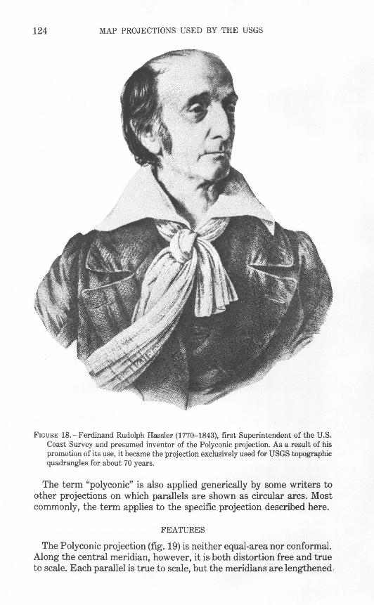
124 MAP PROJECTIONS USED BY THE USGS
FIGURE 18.-Ferdinand Rudolph Hassler (1770-1843), first Superintendent of the U.S. Coast Survey and presumed inventor of the Polyconic projection. As a result of his promotion of its use, it became the projection exclusively used for USGS topographic quadrangles for about 70 years.
The term "polyconic" is also applied generically by some writers to other projections on which parallels are shown as circular arcs. Most commonly, the term applies to the specific projection described here.
FEATURES
The Polyconic projection (fig. 19) is neither equal-area nor conformal. Along the central meridian, however, it is both distortion free and true to scale. Each parallel is true to scale, but the meridians are lengthened
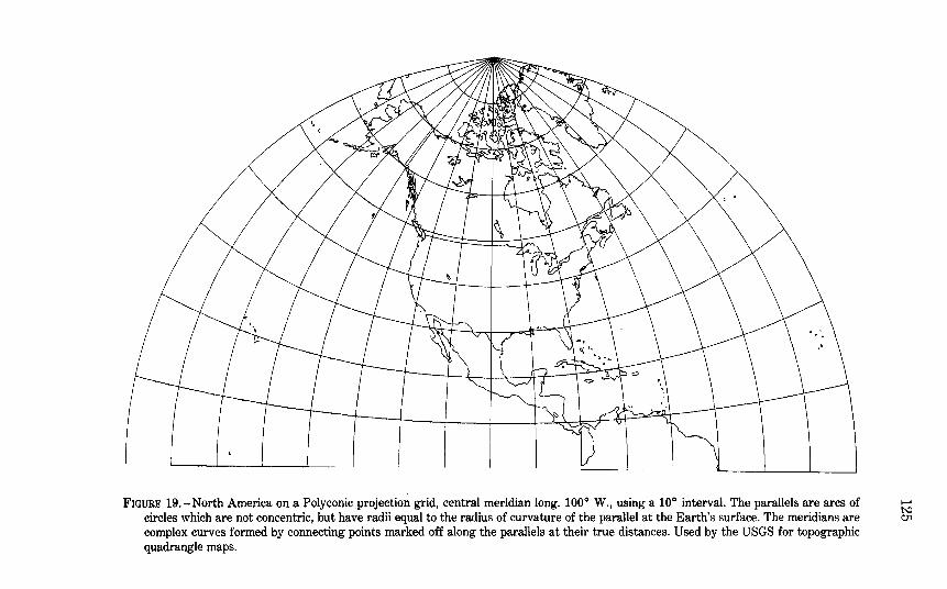
FIGURE 19.-North America on a Polyconic projection grid, central meridian long. 100° W., using a 10° interval. The parallels are arcs of circles which are not concentric, but have radii equal to the radius of curvature of the parallel at the Earth's surface. The meridians are complex curves formed by connecting points marked off along the parallels at their true distances. Used by the USGS for topographic quadrangle maps.
1--l t:-:l 01
126 MAP PROJECTIONS USED BY THE USGS
by various amounts to cross each parallel at the correct position along the parallel, so that no parallel is standard in the sense of having conformality (or correct angles), except at the central meridian. Near the central meridian, which is the case with 11f2-minute quairangles, distortion is extremely small. The Polyconic projection is universal in that tables of rectangular coordinates may be used for any Polyconic projection of the same ellipsoid by merely applying the proper scale and central meridian. U.S. Coast and Geodetic Survey Special Publication No.5 (1900) replaced tables published in 1884 and was often reprinted because of the universality of the projection (the Clarke 18~<) is the reference ellipsoid). Polyconic quadrangle maps prepared to the same scale and for the same central meridian and ellipsoid will fit exactly from north to south. Since they are drawn in practice with straight meridians, they also fit east to west, but discrepancies will ac~~.umulate if mosaicking is attempted in both directions.
The parallels are all circular arcs, with the centers of the a res lying along an extension of the straight central meridian, but these arcs are not concentric. Instead, as noted earlier, the radius of each arc is that of the circle developed from a cone tangent to the sphere or er:osoid at the latitude. For the sphere, each parallel has a radius proportional to the cotangent of the latitude. For the ellipsoid, the radius is slirrhtly different. The Equator is a straight line in either case. Along th~ central meridian, the parallels are spaced at their true intervals. For the sphere, they are therefore equidistant. Each parallel is marked off for meridians equidistantly and true to scale. The points so marked are connected by the curved meridians.
USAGE
As geodetic and coastal surveying began in earnest during the 19th century, the Polyconic projection became a standard, especially for quadrangles. The name of the projection appears on a later r~print of one of the first published USGS topographic quadrangles, ¥Thich appeared in 1886. In 1904, the USGS published tables of rectangular coordinates extracted from an 1884 Coast and Geodetic Surve:T report. They were called "coordinates of curvature," but were actudly coordinates for the Polyconic projection, although the latter term was not used (Gannett, 1904, p. 37 -48).
As a 1928 USGS bulletin of topographic instructions stated (Beaman, 1928, p. 163):
"The topographic engineer needs a projection which is simple in construction, which can be used to represent small areas on any part of the globe, and which, for each small area to which it is applied, preserves shapes, areas, distances, and azimuths in their true relation to the surface of the earth. The polyconic projection meets all these needs and was adopted for the standard topographic map of the United States, in wh:~h the 1°
CONIC MAP PROJECTIONS 127
quadrangle is the largest unit * * * and the 15' quadrangle is th?. average unit. * * * Misuse of this projection in attempts to spread it over large areas- that is, to construct a single map of a large area- has developed serious errors and gros~ exaggeration of details. For example, the polyconic projection is not at all suitable for a singlesheet map of the United States or of a large State, although it has been so employed."
When coordinate plotters and published tables for the SU'.te Plane Coordinate System (SPCS) became available in the late 1f.:JO's, the USGS ceased using the Polyconic for new maps, in favor of the Transverse Mercator or Lambert Conformal Conic projecthns used with the SPCS for the area involved. Some of the qurrirangles prepared on one or the other of these projections have continued to carry the Polyconic designation, however.
The Polyconic projection was also used for the Progressiv~ Military Grid for military mapping of the U.S., until its replacement by the Universal Transverse Mercator grid. There were seven zones, A-G, with central meridians every go west from long. 73° W. (zon€ A), each zone having an origin at lat. 40°30' N. on the central meridian with coordinates X= 1,000,000 yards, y=2,000,000 yards (Deetz and Adams, 1934, p. 87-90). Some USGS quadrangles of the 1930's and 1940's display tick marks according to this grid in yards, and many quadrangles then prepared by the Army Map Service and sold by the USGS show a complete grid pattern.
While quadrangles based on the Polyconic provide low-~istortion mapping of the local areas, the inability to mosaic these quadrangles in all directions without gaps makes them less satisfactory for a larger region. Quadrangles based on the SPCS may be mosaicked over an entire zone, at the expense of increased distortion.
For an individual quadrangle 7112 or 15 minutes of latitude or longitude on a side, the distance of the quadrangle from th~ central meridian of a Transverse Mercator zone or from the standard parallels of a Lambert Conformal Conic zone of the SPCS has much more effect than the type of projection upon the variation in measurement of distances on quadrangles based on the various projections. If the central meridians or standard parallels of the SPCS zones fall on the quadrangle, a change of projection from Polyconic to Transverse Mercator or Lambert Conformal Conic results in a difference of less than 0.001 mm in the measurement of the 700-800 mm diagonals of a 7112-minute quadrangle. If the quadrangle is near the edge of a zone, the discrepancy between measurements of diagonals on two maps of the same quadrangle, one using the Transverse Mercator or Laml'~rt Conformal Conic projection and the other using the Polyconic, can reach about 0.05 mm. These differences are exceeded by variations in expansion and contraction of paper maps, so that these matl,~matical discrepancies apply only to comparisons of stable-base maps.
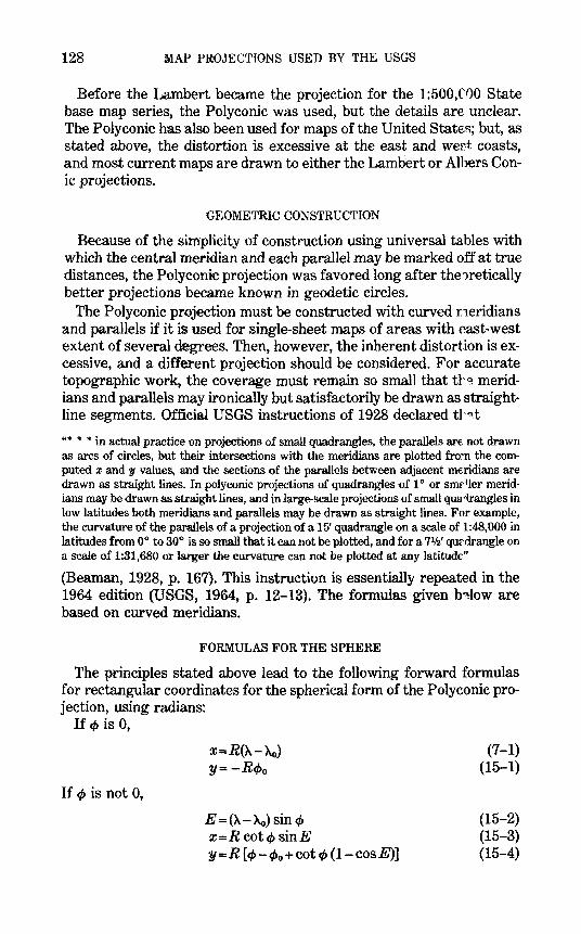
128 MAP PROJECTIONS USED BY THE USGS
Before the Lambert became the projection for the 1:500,('00 State base map series, the Polyconic was used, but the details are unclear. The Polyconic has also been used for maps of the United State-~; but, as stated above, the distortion is excessive at the east and wert coasts, and most current maps are drawn to either the Lambert or Albers Conic projections.
GEOMETRIC CONSTRUCTION
Because of the simplicity of construction using universal tables with which the central meridian and each parallel may be marked off at true distances, the Polyconic projection was favored long after theoretically better projections became known in geodetic circles.
The Polyconic projection must be constructed with curved rneridians and parallels if it is used for single-sheet maps of areas with east-west extent of several degrees. Then, however, the inherent distortion is excessive, and a different projection should be considered. For accurate topographic work, the coverage must remain so small that tl'a. meridians and parallels may ironically but satisfactorily be drawn as straightline segments. Official USGS instructions of 1928 declared tl·~.t
"* "' * in actual practice on projections of small quadrangles, the parallels are not drawn as arcs of circles, but their intersections with the meridians are plotted fro:-n the computed x and y values, and the sections of the parallels between adjacent mt:.ridians are drawn as straight lines. In polyconic projections of quadrangles of 1° or sm~ller meridians may be drawn as straight lines, and in large-scale projections of small qua <l.rangles in low latitudes both meridians and parallels may be drawn as straight lines. For example, the curvature of the parallels of a projection of a 15' quadrangle on a scale of 1:48,000 in latitudes from 0° to 30° is so small that it can not be plotted, and for a 71J2' qurdrangle on a scale of 1:31,680 or larger the curvature can not be plotted at any latitude"
(Beaman, 1928, p. 167). This instruction is essentially repeated in the 1964 edition (USGS, 1964, p. 12-13). The formulas given b~low are based on curved meridians.
FORMULAS FOR THE SPHERE
The principles stated above lead to the following forward formulas for rectangular coordinates for the spherical form of the Polyc:onic projection, using radians:
If t/> is 0,
If¢ is not 0,
X=R(A-Ao) y=-Rt/>o
E=(A-Ao) sin t/> x=R cot tf> sinE y = R [ 4>- t/>0 +cot t/> (1- cos E)]
(7-1) (15-1)
(15-2) (15-3) (15-4)
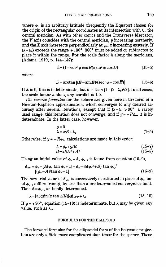
CONIC MAP PROJECTIONS 129
where c/>0 is an arbitrary latitude (frequently the Equator) chosen for· the origin of the rectangular coordinates at its intersection with Ao, the central meridian. As with other conics and the Transversi'?. Mercator, the Y axis coincides with the central meridian, y increasing northerly, and the X axis intersects perpendicularly at cp0 , x increasing easterly. If (A- Ao) exceeds the range ± 180 °, 360 ° must be added or subtracted to place it within the range. For the scale factor h along the meridians, (Adams, 1919, p. 144-147):
h= (1- cos2 cp cos E)/(sin2 cp cos D) (15-5)
where
D =arctan [(E- sin E)/(sec2 cp- cos E)] (15-6)
If cp is 0, this is indeterminate, but h is then [1 +(A- Ao)2/2]. In all cases, the scale factor k along any parallel is 1.0.
The inverse formulas for the sphere are given here in th~ form of a Newton-Raphson approximation, which converges to any desired accuracy after several iterations, except that if IA-Aol >90°, a rarely used range, this iteration does not converge, and if y = - Rcp0 , it is indeterminate. In the latter case, however,
c/>=0 A=xiR+Ao
Otherwise, if y :f.: - Rc/>0 , calculations are made in this order:
A=c/>o+YIR B=x2/R2 +A2
(7-5)
(15-7) (15-8)
Using an initial value of cp, =A, c/>,+1 is found from equation (15-9),
cp,+l = cp,- [A( cp, tan cp, + 1)- cp,- 112( cp, 2 +B) tan cp,.]/ [(c/>, -A)/tan cp, -1] (15-9)
The new trial value of cp,.+l is successively substituted in plac~ of cp,., until c/>,+1 differs from ¢, by less than a predetermined convergence limit. Then cp = c/>,.+1 as finally determined.
A= [arcsin (x tan ¢/R)Jisin¢ + Ao (15-10)
If cp = ± 90°, equation (15-10) is indeterminate, but A may be given any value, such as Ao·
FORMULAS FOR THE ELLIPSOID
The forward formulas for the ellipsoidal form of the Polyconic projection are only a little more complicated than those for the sp},~re. These
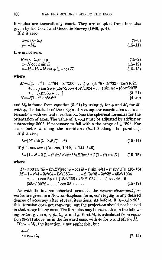
130 MAP PROJECTIONS USED BY THE USGS
formulas are theoretically exact. They are adapted from formulas given by the Coast and Geodetic Survey (1946, p. 4):
If cp is zero:
x=a (A-Ao) y=-Mo
If cp is not zero:
E=(A-Ac,) sin cp x=N cot cp sinE y=M -Mo+N cot cp (1- cos E)
where
(7-6) (15-11)
(15-2) (15-12) (15-13)
M =a[(1-e214- 3e4164- 5e6/256- ... ) cp-(3e2/8+ 3e4/32+45~/1024 + ... ) sin 2c/>+(15e4/256+ 45e6/1024+ ... ) sin 4cp- (35~/:'()72 + ... ) sin 6c/>+ ... ] (3-21)
N = a/(1- e2 sin2cp )112 ( 4-20)
and Mo is found from equation (3-21) by using c/>o for cp and Mo forM, with c/>o the latitude of the origin of rectangular coordinates at its intersection with central meridian Ac,. See the spherical formulas for the orientation of axes. The value of (A- Ac,) must be adjusted by adcing or subtracting 360°, if necessary to fall within the range of ± 18(] o. For scale factor h along the meridians (k= 1.0 along the parallels):
If cp is zero,
h = [M + 112 (A- Ac,)2]/(1- el)
If cp is not zero (Adams, 1919, p. 144-146),
h= [1-el+ 2 (1- e2 sin2 cp) sin2 1/zE/tan2 cp]/[(1- e2) cosD]
where
(15-14)
(15-15)
D= arctan {(E -sinE)/[sec2 cp-cosE -el sin2 cp/(1-el sin2 cp)]} (15-16) M = 1-:- el/4- 3e4/64- 5~/256- ... -2 (3e2/8 + 3e4132 + 45e6/1024
+ ... ) cos 2¢+ 4 (15e4/256+ 45e6/1024 + ... ) cos 4cp- 6 (35e6/ 3072 + ... ) cos 6cp + . . . . (15-17)
As with the inverse spherical formulas, the inverse ellipsoidal formulas are given in a Newton-Raphson form, converging to any desired degree of accuracy after several iterations. As before, if I A- Ac,l > 90°, this iteration does not converge, but the projection should not t~ used in that range in any case. The formulas may be calculated in the following order, given a, e, c/>o, Ac,, x, and y. First Mo is calculated from equation (3-21) above, as in the forward case, with c/>o for cp and Mo f1r M.
If y = - Mo, the iteration is not applicable, but
c/>=0 A=xla+Ac, (7-12)
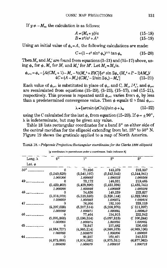
CONIC MAP PROJECTIONS
If y ::1= - Mo, the calculation is as follows:
A=(Mo+Y)Ia B=x2/a2 +A2
131
(15-18) (15-19)
Using an initial value of cl>n =A, the following calculations are made:
C = (1- e2 sin2 cl>n)112 tan cl>n (15-20)
ThenMn andMn' are found from equations (3-21) and (15-17) above, using cf>n for cp, Mn forM, andMn' forM. LetMa=Mn/a.
cl>n+l = cl>n- [A(CM" + 1)-M" -lf2(Ma2 +B)C]I[e2 sin 2c~>n (Ma 2 +1? -2AM")I 4C +(A -Ma) (CMn'- 2/sin 2cpn)-Mn'] (15-21)
Each value of cl>n+t is substituted in place of cl>n, and C, Mn, I~fn', and cf>n+t are recalculated from equations (15-20), (3-21), (15-17), f.nd (15-21), respectively. This process is repeated until cl>n+t varies fron cl>n by less than a predetermined convergence value. Then cp equals tl· ~ final cf>n+t·
A= [arcsin (xC/a)]/sin cp+ Ao (15-22)
using the C calculated for the last cf>n from equation (15-20). If cp = ± 90°, A. is indeterminate, but may be given any value.
Table 18lists rectangular coordinates for a band 3° on either side of the central meridian for the ellipsoid extending from lat. 23° to 50° N. Figure 19 shows the graticule applied to a map of North America.
TABLE 18.-Polyconic Projection:Rectangular coordinates/or the Clarke 1866 ellipsoid
[y coordinates in parentheses under x coordinates. Italic indicates h]
Long. A oo 10 20 30
Lat. t/J
50 ° --------- 0 71,696 143,379 215,037 (5,540,628) (5,541,107) (5,542,545) (5,544,941)
1.000000 1.000063 1.000252 1.000568 49 ---------- 0 73,172 146,331 219,465
(5,429,409) (5,429,890) (5,431,336) (5,433, 7 45) 1.000000 1.000066 1.000263 1.000592
48 ---------- 0 74,626 149,239 223,827 (5,318,209) (5,318,693) (5,320,144) (5,322,564)
1.000000 1.000068 1.000274 1.000616 4 7 ---------- 0 76,056 152,100 228,119
(5,207,028) (5,207,514) (5,208,970) (f .211,397) 1.000000 1.000071 1.000284 1.000640
46 ---------- 0 77,464 154,915 . 232,342 (5,095,868) (5,096,354) (5,097,813) (f 100,244)
1.000000 1.000074 1.000295 1.000664 45 ---------- 0 78,847 157,682 236,493
(4,984, 727) (4,985,214) (4,986,673) (4,989,106) 1.000000 1.000076 1.000306 1.000688
44 ---------- 0 80,207 160,401 240,572 (4,873,606) (4,874,092) (4,875,551) (4,877,982)
1.000000 1.000079 1.000316 1.000712
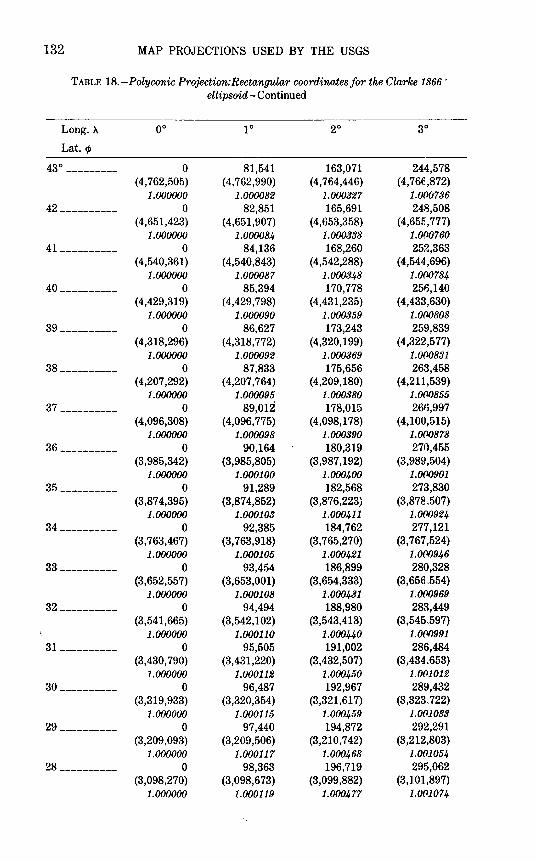
132 MAP PROJECTIONS USED BY THE USGS
TABLE 18. -Polyconic Projection: Rectangular coordinates for the Clarke 1866' ellipsoid- Continued
Long.>. oo 10 20 30
Lat.~
43 ° --------- 0 81,541 163,071 244,578 (4,762,505) (4,762,990) (4,764,446) (4,766,872)
1.000000 1.000082 1.000327 1.000736
42 ---------- 0 82,851 165,691 248,508 (4,651,423) (4,651,907) (4,653,358) (4,655,777)
1.000000 1.000084 1.000338 1.000760 41 __________ 0 84,136 168,260 252,363
(4,540,361) (4,540,843) (4,542,288) (4,544,696) 1.000000 1.000087 1.000348 1.000784
40 ---------- 0 85,394 170,778 256,140 (4,429,319) (4,429,798) (4,431,235) (4,433,630)
1.000000 1.000090 1.000359 1.000808
39 ---------- 0 86,627 173,243 259,839 (4,318,296) (4,318,772) (4,320,199) (4,322,577)
1.000000 1.000092 1.000369 1.000831
38 ---------- 0 87,833 175,656 263,458 (4,207,292) (4,207,764) (4,209,180) (4,211,539)
1.000000 1.000095 1.000380 1.000855
37---------- 0 89,012 178,015 266,997 (4,096,308) (4,096,775) (4,098,178) (4,100,515)
1.000000 1.000098 1.000390 1.000878
36 ---------- 0 90,164 180,319 270,455 (3,985,342) (3,985,805) (3,987,192) (3,989,504)
1.000000 1.000100 1.000400 1.000901
35 ---------- 0 91,289 182,568 273,830 (3,87 4,395) (3,87 4,852) (3,876,223) (3,878 .507)
1.000000 1.000103 1.000411 1.000924
34 ---------- 0 92,385 184,762 277,121 (3,763,467) (3, 763,918) (3, 765,270) (3,767,524)
1.000000 1.000105 1.000421 1.0(1()946
33 ---------- 0 93,454 186,899 280,328 (3,652,557) (3,653,001) (3,654,333) (3,656 .554)
1.000000 1.000108 1.000431 1.000969
32 ---------- 0 94,494 188,980 288,449 (3,541,665) (3,542,102) (3,543,413) (3,545.597)
1.000000 1.000110 1.000440 1.0(1()991 31 __________ 0 95,505 191,002 286,484
(3,430,790) (3,431,220) (3,432,507) (3,434~653)
1.000000 1.000112 1.000450 1.0(1.1012
30 ---------- 0 96,487 192,967 289,432 (3,319,933) (3,320,354) (3,321,617) (3,323. 722)
1.000000 1.000115 1.000459 1.001033
29 ---------- 0 97,440 194,872 292,291 (3,209,093) (3,209,506) (3,210,742) (3,212,803)
1.000000 1.000117 1.000468 1.001054
28 ---------- 0 98,363 196,719 295,062 (3,098,270) (3,098,673) (3,099,882) (3,101,897)
1.000000 1.000119 1.000477 1.0(11074
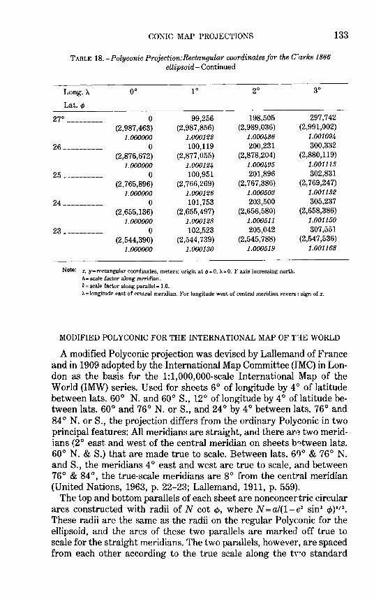
CONIC MAP PROJECTIONS 133
TABLE 18.-Poly conic Projection: Rectangular coordinates for the C'a,rke 1866 ellipsoid- Continued
Long. >. oo 10 20 go
Lat. 4>
27° --------- 0 99,256 198,505 297,742 (2,987,463) (2,987 ,856) (2,989,036) (2,991,002)
1.000000 1.000122 1.000486 1.001094
26 ---------- 0 100,119 200,231 300,332 (2,876,672) (2,877,055) (2,878,204) (2,880,119)
1.000000 1.000124 1.000495 1.001113
25 ---------- 0 100,951 201,896 302,831 (2, 765,896) (2, 766,269) (2,767,386) (2,769,247)
1.000000 1.000126 1.000503 1.001132
24 ---------- 0 101,753 203,500 305,237 (2,655,136) (2,655,497) (2,656,580) (2,658,386)
1.000000 1.000128 1.000511 1.001150
23 ---------- 0 102,523 205,042 307,551 (2,544,390) (2,544, 739) (2,545,788) (2,547,536)
1.000000 1.000130 1.000519 1.001168
Note: x, y=rectangular coordinates, meters; origin at <f>=O, >.=0. Y axis increasing north. h= scale factor along meridian. k=scale factor along parallel= 1.0. A= longitude east of central meridian. For longitude west of central meridian revers'~ sign of x.
MODIFIED POLYCONIC FOR THE INTERNATIONAL MAP OF T"IE WORLD
A modified Polyconic projection was devised by Lallemand of France and in 1909 adopted by the International Map Committee (JMC) in London as the basis for the 1:1,000,000-scale International Map of the World (IMW) series. Used for sheets 6 o of longitude by 4 o of latitude between lats. 60° N. and 60° S., 12° of longitude by 4 o of latitude between lats. 60° and 76° N. or S., and 24° by 4° between lats. 76° and 84° N. or S., the projection differs from the ordinary Polyconic in two principal features: All meridians are straight, and there are two meridians (2° east and west of the central meridian on sheets b~tween lats. 60° N. & S.) that are made true to scale. Between lats. 60° & 76° N. and S., the meridians 4 ° east and west are true to scale, and between 76° & 84 °, the true-scale meridians are 8° from the central meridian (United Nations, 1963, p. 22-23; Lallemand, 1911, p. 559).
The top and bottom parallels of each sheet are nonconcertric circular arcs constructed with radii of N cot cp, where N = a/(1- e2 sin2 c/>) 112
•
These radii are the same as the radii on the regular Polyconic for the ellipsoid, and the arcs of these two parallels are marked off true to scale for the straight meridians. The two parallels, however, are spaced from each other according to the true scale along the tFo standard
134 MAP PROJECTIONS USED BY THE USGS
meridians, not according to the scale along the central meridian, which is slightly reduced. The approximately 440 mm true length of th~ central meridian at the map scale is thereby reduced by 0.270 to 0.076 mm, depending on the latitude of the sheet. Other parallels of lat. ¢ are circular arcs with radii N cot ¢, intersecting the meridians which are true to scale at the correct points. The parallels strike other meridians at geometrically fixed locations which slightly deviate from the true scale on meridians as well as parallels.
With this modified Polyconic, as with USGS quadrangles baEed on the rectified Polyconic, adjacent sheets exactly fit together not only north to south~ but east to west. There is still a gap when mosaicking in all directions, in that there is a gap between each diagonal sheet and either one or the other adjacent sheet.
In 1962, a U.N. conference on the IMW adopted the Lambert Conformal Conic and Polar Stereographic projections to replace the modified Polyconic (United Nations, 1963, p. 9-10). The USGS has prepared a number of sheets for the IMW series over the years according to the projection officially in use at the time.
AZIMUTHAL MAP PROJECTIONS
A third very important group of map projections, some of which have been known for 2,000 years, consists of five major azimuthal (or zenithal) projections and various less-common forms. While cylindrical and conic projections are related to cylinders and coil es wrapped around the globe representing the Earth, the azimuthal projections are formed onto a plane which is usually tangent to the globe at either pole, the Equator, or any intermediate point. These variations are called the polar, equatorial (or meridian or meridional), and oblique (or horizon) aspects, respectively. Some azimuthals are true perspective projections; others are not. Although perspective cylindrical and conic projections are much less used than those which are not perE·nective, the perspective azimuthals are frequently used and have valu:tble properties. Complications arise when the ellipsoid is involved, but it is used only in special applications that are discussed below.
As stated earlier, azimuthal projections are characterized by the fact that the direction, or azimuth, from the center of the rrojection to every other point on the map is shown correctly. In addition, on the spherical forms, all great circles passing through the center of the projection are shown as straight lines. Therefore, the shortest route from this center to any other point is shown as a straight line. Ttis fact made some of these projections especially popular for maps a'"l flight and radio transmission became commonplace.
The five principal azimuthals are as follows: (1) Orthographic. A true perspective, in which the Earth is projected
from an infinite distance onto a plane. The map looks like a globe, thus stressing the roundness of the Earth.
(2) Stereographic. A true perspective in the spherical fo:--m, with the point of perspective on the surface of the sphere at a point exactly opposite the point of tangency for the plane, or opposite the center of the projection, even if the plane is secant. This projection is conformal for sphere or ellipsoid, but the ellips')idal form is not truly perspective.
(3) Gnomonic. A true perspective, with the Earth projected from the center onto the tangent plane. All great circles, not merely those passing through the center, are shown as straight lines on the spherical form. Since the Gnomonic projection has n':lt been used by the USGS, it is not discussed in detail.
(4) Lambert Azimuthal Equal-Area. Not a true perspective. Areas are correct, and the overall scale variation is less than t\at found on the major perspective azimuthals.
135
136 MAP PROJECTIONS USED BY THE USGS
(5) Azimuthal Equidistant. Not a true perspective. Distances from the center of the projection to any other point are shown cc~rectly. Overall scale variation is moderate compared to the pe•spective azimuthals.
A sixth azimuthal projection of increasing interest in the space age is the general vertical perspective (resembling the Orthographic), projecting the Earth from any point in space, such as a satellite, onto a tangent or secant plane. It is used primarily in derivations and pictorial representations and has not been used by the Geological Surv~y for published maps. Therefore, it is not discussed in this bulletin.
As a group, the azimuthals have unique esthetic qualities while remaining functional. There is a unity and roundness of the Earth on each (except perhaps the Gnomonic) which is not as apparent on cylindrical and conic projections.
The simplest forms of the azimuthal projections are the polar aEpects, in which all meridians are shown as straight lines radiating at the;r true angles from the center, while parallels of latitude are circles, concentric about the pole. The difference is in the spacing of the parallels. Table 19lists for all five of the above azimuthals the radius of eve..,.y 10° of latitude on a sphere of radius 1.0 unit, centered on the NorU Pole. Scale factors and maximum angular deformation are also shown. The distortion is the same for the oblique and equatorial aspects at the same angular distance from the center of the projection, except that h and k are along and perpendicular to, respectively, radii from the center, not necessarily along meridians or parallels.
There are two principal drawbacks to the azimuthals. First, th~y are more difficult to construct than the cylindricals and the conics, except for the polar aspects. This drawback was more applicable, howe"rer, in the days before computers and plotters, but it is still more difficult to prepare a map having complex curves between plotted coordinates than it is to draw the entire graticule with circles and straight lines. Nevertheless, an increased use of azimuthal projections in atlases and for other published maps may be expected.
Secondly, most azimuthal maps do not have standard parallels or standard meridians. Each map. has only one standard point: the center (except for the Stereographic, which may have a-standard circle). Thus, the azimuthals are suitable for minimizing distortion in a somewhat circular region such as Antarctica, but not for an area with predominant length in one direction.
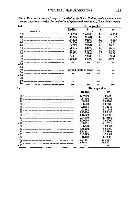
AZIMUTHAL MAP PROJECTIONS 137
TABLE 19.-Comparison of major azimuthal projections: Radius, scale factors, maximum angular distortion/or projection of sphere with radius 1.0, North Polar aspect
Lat. Orthographic Radius h k w
90° ----------------------------80 ____________________________ _ 70 ____________________________ _ 60 ____________________________ _ 50 ____________________________ _ 40 ____________________________ _ 30 ____________________________ _ 20 ____________________________ _ 10 ____________________________ _ o ____________________________ _
- 10 ------------------------------ 20 ------------------------------ 30 -----------------------------
0.00000 .17365 .34202 .50000 .64279 .76604 .86603 .93969 .98481
1.00000
1.00000 .98481 .93969 .86603 .76604 .64279 .50000 .34202 .17365 .00000
1.0 1.0 1.0 1.0 1.0 1.0 1.0 1.0 1.0 1.0
0.000° .877
3.563 8.234
15.23 25.12 38.94 58.72 89.51
180.0
- 40 ----------------------------- (beyond limits of map) - 50 ------------------------------ 60 ------------------------------ 70 ------------------------------- 80 ------------------------------ 90 -----------------------------
Lat.
90° -----------------------------------80 ___________________________________ _ 70 ___________________________________ _ 60 ___________________________________ _ 50 ___________________________________ _ 40 ___________________________________ _ 30 ___________________________________ _ 20 ___________________________________ _ 10 ___________________________________ _ o ___________________________________ _
- 10 ------------------------------------- 20 ------------------------------------- 30 ------------------------------------- 40 ------------------------------------- 50 ------------------------------------- 60 ------------------------------------- 70 ------------------------------------- 80 ------------------------------------- 90 ------------------------------------
Stereographi(> Radius k*
0.00000 .17498 .35263 .53590 .72794 .93262
1.15470 1.40042 1.67820 2.00000 2.38351 2.85630 3.46410 4.28901 5.49495 7.46410
11.3426 22.8601
1.00000 1.00765 1.03109 1.07180 1.13247 1.21744 1.33333 1.49029 1.70409 2.00000 2.42028 3,03961 4.00000 5,59891 8,54863
14.9282 33,1634
131.646 00
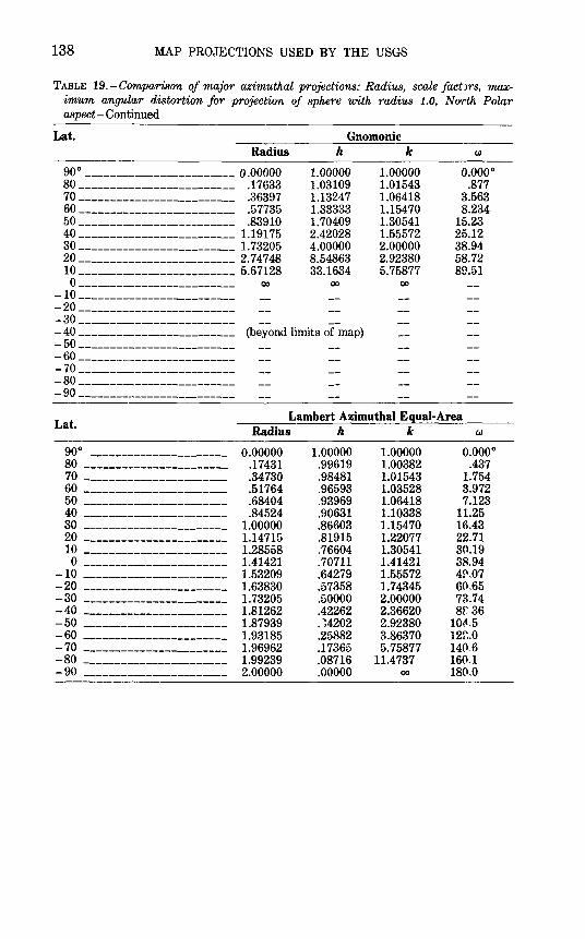
138 MAP PROJECTIONS USED BY THE USGS
TABLE 19.-Comparison of major azimuthal projections: Radius, scale fact,Jrs, maximum angular distortion for projection of sphere with radius 1.0, North Polar aspect- Continued
Lat. Gnomonic Radius
90°------------------------ 0.00000 80 ------------------------- .17633 70 ------------------------- .36397 60 ------------------------- .57735 50------------------------- .83910 40------------------------- 1.19175 30 ------------------------- 1. 73205 20 ------------------------- 2. 7 4 7 48 10 ------------------------- 5. 67128
0 ------------------------- 00
-10-------------------------- 20 -------------------------- 30 -------------------------
h
1.00000 1.03109 1.13247 1.33333 1.70409 2.42028 4.00000 8.54863 33.1634
00
-40 ------------------------- (beyond limits of map) - 50 -------------------------- 60 -------------------------- 70 -------------------------- 80 -------------------------- 90 --------------------------
k
1.00000 1.01543 1.06418 1.15470 1.30541 1.55572 2.00000 2.92380 5.75877
00
w
0.000° .877
3.563 8.234
15.23 25.12 38.94 58.72 8t'.51
Lat. Lambert Azimuthal Equal-Area
90° ----------------------80 -----------------------70 -----------------------60 -----------------------50 -----------------------40 -----------------------30 -----------------------20 -----------------------10 -----------------------0 ----------------------
-10 ------------------------20 ------------------------30 ------------------------40 ------------------------50 ------------------------60 ------------------------70 ------------------------80 ------------------------90 -----------------------
Radius h k w
0.00000 .17431 .34730 .51764 .68404 .84524
1.00000 1.14715 1.28558 1.41421 1.53209 1.63830 1.73205 1.81262 1.87939 1.93185 1.96962 1.99239 2.00000
1.00000 .99619 .98481 .96593 .93969 .90631 .86603 .81915 .76604 .70711 .64279 .57358 .50000 .42262 .~4202 .25882 .17365 .08716 .00000
1.00000 1.00382 1.01543 1.03528 1.06418 1.10338 1.15470 1.22077 1.30541 1.41421 1.55572 1.74345 2.00000 2.36620 2.92380 3.86370 5.75877
11.4737 00
0.000° .437
1.754 3.972 7.123
11.25 16.43 22.71 30.19 38.94 4!'.07 60.65 73.74 8r 36
10.;1..5 12r..o 140.6 160.1 180.0
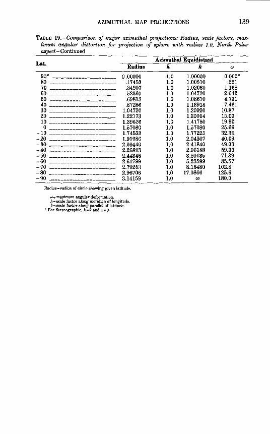
AZIMUTHAL MAP PROJECTIONS 139
TABLE 19.-Comparison of major azimuthal projections: Radius, scale factors, maximum angular distortion for projection of sphere with radius 1.0, North Polar aspect- Continued
Lat.
goo ----------------------80 -----------------------70 -----------------------60 -----------------------60 -----------------------40 -----------------------30 -----------------------20 -----------------------10 -----------------------0 ----------------------
-10 ------------------------20 ------------------------30 ------------------------40 ------------------------ 50 -------------------------60 ------------------------70 ------------------------80 ------------------------90 -----------------------
Radius
0.00000 .17453 .34907 .52360 .69813 .87266
1.04720 1.22173 1.39626 1.57080 1.74533 1.91986 2.09440 2.26893 2.44346 2.61799 2.79253 2.96706 3.14159
Radius= radius of circle showing given latitude.
w=maximum angular deformation. h =scale factor along meridian of longitude. k =scale factor along parallel of latitude.
• For Stereographic, h-k and w=O.
Azimuthal Equidistant h k
1.0 1.00000 1.0 1.00510 1.0 1.02060 1.0 1.04720 1.0 1.08610 1.0 1.13918 1.0 1.20920 1.0 1.30014 1.0 1.41780 1.0 1.57080 1.0 1.77225 1.0 2.04307 1.0 2.41840 1.0 2.96188 1.0 3.80135 1.0 5.23599 1.0 8.16480 1.0 17.0866 1.0 00
w
0.000° .291
1.168 2.642 4.731 7.461
10.87 15.00 19.90 25.66 32.35 40.09 49.03 59.36 71.39 85.57
102.8 125.6 180.0

16. ORTHOGRAPHIC PROJECTION
SUMMARY
• Azimuthal. • All meridians and parallels are ellipses, circles, or straight lines. • Neither conformal nor equal-area. • Closely !"esembles a globe in appearance, since it is a perspective rrojection from
infinite distance. • Only one hemisphere can be shown at a time. • Much distortion near the edge of the hemisphere shown. • No distortion at the center only. • Directions from the center are true. • Radial scale factor decreases as distance increases from the center. • Scale in the direction of the lines of latitude is true in the polar aspect. • Used chiefly for pictorial views. • Used only in the spherical form. • Known by Egyptians and Greeks 2,000 years ago.
HISTORY
To the layman, the best known perspective azimuthal projection is the Orthographic, although it is the least useful for measurements. While its distortion in shape and area is quite severe near the edges, and only one hemisphere may be shown on a single mar:' the eye is much more willing to forgive this distortion than to forgivf~ that of the Mercator projection because the Orthographic projectior makes the map look very much like a globe appears, especially in the oblique aspect.
The Egyptians were probably aware of the Orthographic projection, and Hipparchus of Greece (2nd century B.C.) used the equatorial aspect for astronomical calculations. Its early name was "analem1na," a name also used by Ptolemy, but it was replaced by "orthographic" in 1613 by Francois d' Aiguillon of Antwerp. While it was also used by Indians and Arabs for astronomical purposes, it is not known to have b~en used for world maps older than 16th-century works by Albr~cht Dfirer (1471-1528), the German artist and cartographer, who prt'rlared polar and equatorial versions (Keuning, 1955, p. 6).
FEATURES
The point of perspective for the Orthographic projectior is at an infinite distance, so that the meridians and parallels are projected onto the tangent plane with parallel projection lines. All meridians and parallels are shown as ellipses, circles, or straight lines.
141
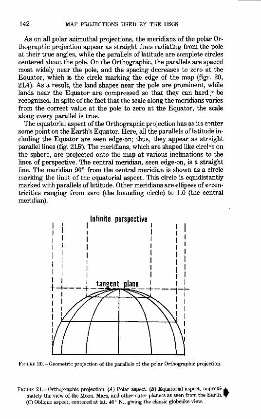
142 MAP PROJECTIONS USED BY THE USGS
As on all polar azimuthal projections, the meridians of the polar Orthographic projection appear as straight lines radiating from the pole at their true angles, while the parallels of latitude are complete circles centered about the pole. On the Orthographic, the parallels are spaced most widely near the pole, and the spacing decreases to zero at the Equator, which is the circle marking the edge of the map (figL 20, 21A). As a result, the land shapes near the pole are prominent, while lands near the Equator are compressed so that they can hard':T be recognized. In spite of the fact that the scale along the meridians varies from the correct value at the pole to zero at the Equator, the scale along every parallel is true.
The equatorial aspect of the Orthographic projection has as its C~'~nter some point on the Earth's Equator. Here, all the parallels of latitude including the Equator are seen edge-on; thus, they appear as str~.ight parallel lines (fig. 21B). The meridians, which are shaped like circl~s on the sphere, are projected onto the map at various inclinations to the lines of perspective. The central meridian, seen edge-on, is a straight line. The meridian 90° from the central meridian is shown as a circle marking the limit of the equatorial aspect. This circle is equidistantly marked with parallels of latitude. Other meridians are ellipses of e~centricities ranging from zero (the bounding circle) to 1.0 (the central meridian).
I I I
Infinite I
perspective I
I I I I I I I
tJ----+ _t_!ngent
I I I I I I I 1 I
plane I 1 I
I I I I I
---+--~-~ ~~~---~~~~ I :
I I I I
I I I I
~+----+-------~-----~--~~ I I I
FIGURE 20.- Geometric projection of the parallels of the polar Orthographic projection.
FIGURE 21.-0rthographic projection. (A) Polar aspect. (B) Equatorial aspect, approxi- A. mately the view of the Moon, Mars, and other outer planets as seen from the Earth. 19" (C) Oblique aspect, centered at lat. 40° N., giving the classic globelike view.
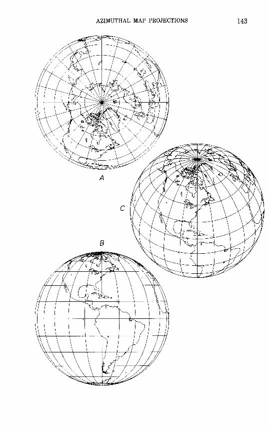
AZIMUTHAL MAP PROJECTIONS 143
144 MAP PROJECTIONS USED BY THE USGS
The oblique Orthographic projection, with its center somew}' ~re between the Equator and a pole, gives the classic globelike appe~.rance; and in fact an oblique view, with its center near but not on the Equator or pole, is often preferred to the equatorial or polar aspect for rictorial purposes. On the oblique Orthographic, the only straight line is the central meridian, if it is actually portrayed. All parallels of latitude are ellipses with the same eccentricity (fig. 21C). Some of these ellir<;\es are shown completely and some only partially, while some cannot be shown at all. All other meridians are also ellipses of varying eccentricities. No meridian appears as a circle on the oblique aspect.
The intersection of any given meridian and parallel is shown on an Orthographic projection at the same distance from the central meridian, regardless of whether the aspect is oblique, polar, or equ:.ttorial, provided the same central meridian and the same scale are mair~ained. Scale and distortion, as on all azimuthal projections, change orly with the distance from the center. The center of projection has no dist,ortion, but the outer regions are compressed, even though the scale is true along all circles drawn about the center. (These circles are not "standard" lines because the scale is true only in the direction followec by the line.)
USAGE
The Orthographic projection seldom appears in atlases, excE'~t as a globe in relief without meridians and parallels. When it does appear, it provides a striking view. Richard Edes Harrison has used the. Orthographic for several maps in an atlas of the 1940's partially based on this projection. Frank Debenham (1958) used photographerl relief globes extensively in The Global Atlas, and Rand MeN ally has done likewise in their world atlases since 1960. The USGS has used it occasionally as a frontispiece or end map (USGS, 1970; Thompson, 1979), but it also provided a base for definitive maps of voyages of discovery across the North Atlantic (USGS, 1970, p. 133).
It became especially popular during the Second World War when there was stress on the global nature of the conflict. With som~ space flights of the 1960's, the first photographs of the Earth frmn space renewed consciousness of the Orthographic concept.
GEOMETRIC CONSTRUCTION
The three aspects of the Orthographic projection may be graphically constructed with an adaptation of the draftsman's technique sh':lwn by Raisz (1962, p. 180). Referring to figure 22, circle A is drawn for the polar aspect, with meridians marked at true angles. Perpendiculars are
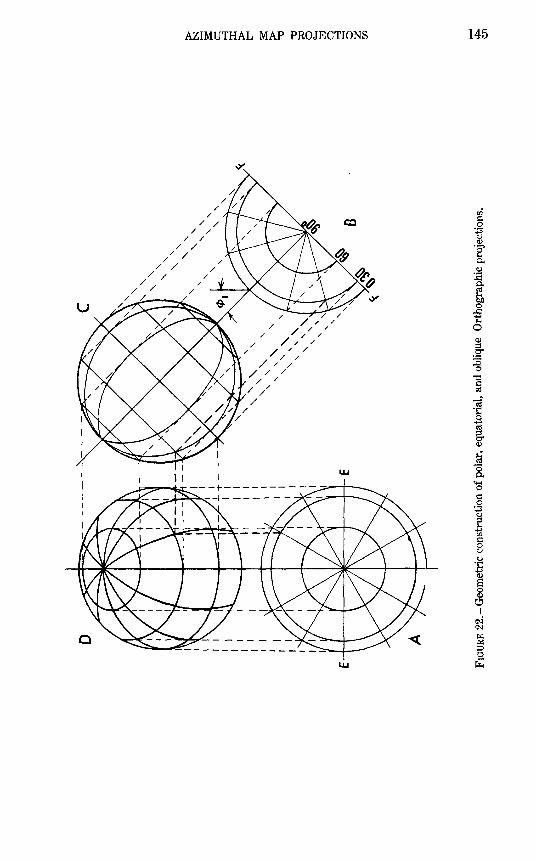
AZIMUTHAL MAP PROJECTIONS 145
~ 0
:0 e.,) Q)
·s ""' 0..
:E
"" ~ 0
..c: ~
""' 0 Q)
-~ :0 0
"'e s:: ~
cJ ·~ 0 ~ ~ g. Q)
ti w 0
0.. <+-< 0 s:: :3 e ~ rn s:: 0 <:,)
e.,)
·~ ~ Q) e 0 Q)
c:..? I
c-3 C'l r.J P:: 0 C!)
w ~
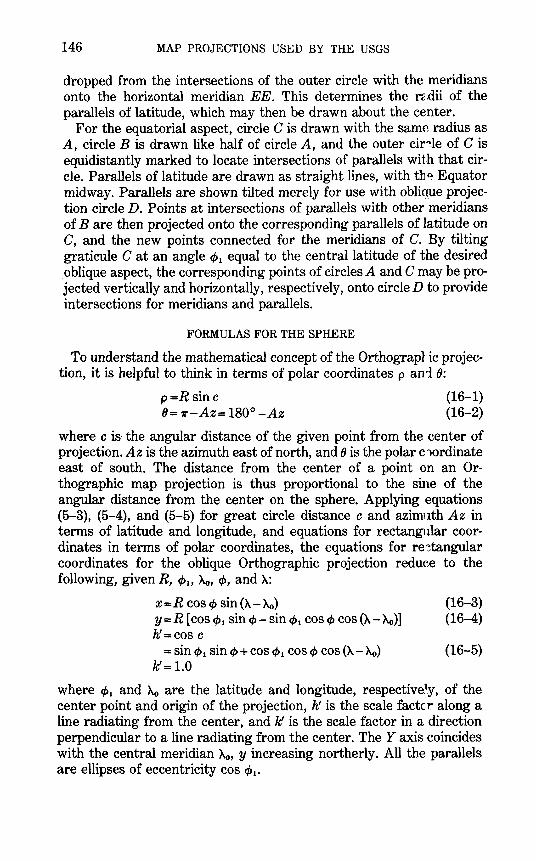
146 MAP PROJECTIONS USED BY THE USGS
dropped from the intersections of the outer circle with the meridians onto the horizontal meridian EE. This determines the rz.dii of the parallels of latitude, which may then be drawn about the center.
For the equatorial aspect, circle C is drawn with the same radius as A, circle B is drawn like half of circle A, and the outer cir~le of Cis equidistantly marked to locate intersections of parallels with that circle. Parallels of latitude are drawn as straight lines, with th~ Equator midway. Parallels are shown tilted merely for use with obliaue projection circle D. Points at intersections of parallels with other meridians of B are then projected onto the corresponding parallels of latitude on C, and the new points connected for the meridians of C. By tilting graticule C at an angle c/> 1 equal to the central latitude of the desired oblique aspect, the corresponding points of circles A and C may be projected vertically and horizontally, respectively, onto circleD to provide intersections for meridians and parallels.
FORMULAS FOR THE SPHERE
To understand the mathematical concept of the Orthographc projection, it is helpful to think in terms of polar coordinates p ani ():
p=R sine B= 1r-Az= 180° -Az
(16-1) (16-2)
where c is· the angular distance of the given point from the center of projection. Az is the azimuth east of north, and() is the polar c1ordinate east of south. The distance from the center of a point on an Orthographic map projection is thus proportional to the sine of the angular distance from the center on the sphere. Applying equations (5-3), (5-4), and (5-5) for great circle distance c and azimuth Az in terms of latitude and longitude, and equations for rectangular coordinates in terms of polar coordinates, the equations for re,~tangular coordinates for the oblique Orthographic projection reduce to the following, given R, c/>11 Ao, cp, and :A:
x=R cos cJ> sin (:A- Ao) y=R [cos c/>1 sin cp- sin c/>1 cos cp cos (:A- Ao)] hf=COS C
= sin c/>1 sin cJ> +cos c/>1 cos cJ> cos (:A- Ao) k'= 1.0
(16-3) (16-4)
(16-5)
where c/>1 and Ao are the latitude and longitude, respective~y, of the center point and origin of the projection, h! is the scale factc r along a line radiating from the center, and k' is the scale factor in a direction perpendicular to a line radiating from the center. TheY axis coincides with the central meridian Ao, y increasing northerly. All the parallels are ellipses of eccentricity cos c/>1•
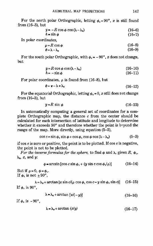
AZIMUTHAL MAP PROJECTIONS 147
For the north polar Orthographic, letting c/1 1 = 90°, x is still found from (16-3), but
Y= -R cos c/1 cos (>-.->.o) h= sin c/1
In polar coordinates, p =R COSc/J 0=>-.->.o
(16-6) (16-7)
(16-8) (16-9)
For the south polar Orthographic, with c/1 1 = - 90°, x does not change, but
y = R cos c/1 cos (>-.- >.o) h= -sin c/1
For polar coordinates, p is found from (16-8), but
0=71"-A+Ao
(16-10) (16-11)
(16-12)
For the equatorial Orthographic, letting c/1 1 = 0, x still does not change from (16-3), but
y=R sin c/1 (16-13)
In automatically computing a general set of coordinates for a complete Orthographic map, the distance c from the center should be calculated for each intersection of latitude and longitude to determine whether it exceeds 90° and therefore whether the point is b~yond the range of the map. More directly, using equation (5-3),
cos c =sin c/1. sin c/1 +cos c/1. cos c/1 cos(>-.- >.o) (5-3)
if cos c is zero or positive, the point is to be plotted. If cos c is negative, the point is not to be plotted.
For the inverse formulas for the sphere, to find c/1 and }.., given R, c/1., Ao, x, andy:
c/1 =arcsin [cos c sin c/1 1 + (y sin c cos c/1 1/ p )] (16-14)
But if p = 0, c/1 = c/J •• If c~J. is not ± 90°,
>-.=>.o+ arctan [x sin c/(p cos c/1 1 cos c-y sin cPt sin c)] (16-15) If c/1. is 90°,
>-.=>.o+arctan [xl( -y)] (16-16)
>-.=>.o+arctan (xly) (16-17)
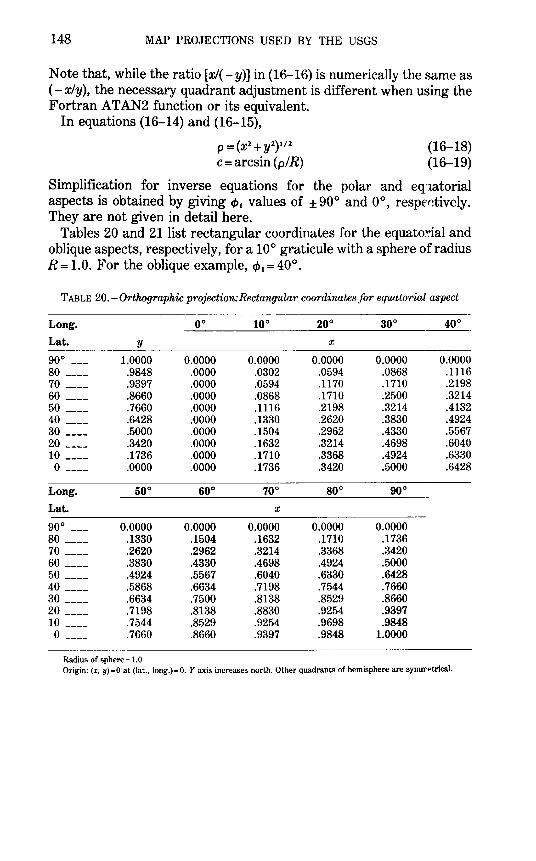
148 MAP PROJECTIONS USED BY THE USGS
Note that, while the ratio [x/( -y)] in (16-16) is numerically the same as (- xly), the necessary quadrant adjustment is different when using the Fortran ATAN2 function or its equivalent.
In equations (16-14) and (16-15),
P = (x2 + y2)1'2 c =arcsin (p/R)
(16-18) (16-19)
Simplification for inverse equations for the polar and eq'Iatorial aspects is obtained by giving c/> 1 values of ± 90° and 0°, respE'r!tively. They are not given in detail here.
Tables 20 and 21list rectangular coordinates for the equato~ial and oblique aspects, respectively, for a 10° graticule with a sphere of radius R = 1.0. For the oblique example, c/> 1 = 40°.
TABLE 20.-0rthographic projection: Rectangular coordinates for equatorial aspect
Long. oo 10° 20° 30° 40°
Lat. y X
90° --- 1.0000 0.0000 0.0000 0.0000 0.0000 0.0000 80 ---- .9848 .0000 .0302 .0594 .0868 .1116 70 ---- .9397 .0000 .0594 .1170 .1710 .2198 60 ---- .8660 .0000 .0868 .1710 .2500 .3214 50 ---- .7660 .0000 .1116 .2198 .3214 .4132 40 ---- .6428 .0000 .1330 .2620 .3830 .4924 30 ---- .5000 .0000 .1504 .2962 .4330 .5567 20 ---- .3420 .0000 .1632 .3214 .4698 .6040 10 ---- .1736 .0000 .1710 .3368 .4924 .6330 0 ---- .0000 .0000 .1736 .3420 .5000 .6428
Long. 50° 60° 70° 80° goo
Lat. X
goo --- 0.0000 0.0000 0.0000 0.0000 0.0000 80 ---- .1330 .1504 .1632 .1710 .1736 70 ---- .2620 .2962 .3214 .3368 .3420 60 ---- .3830 .4330 .4698 .4924 .5000 50 ---- .49.24 .5567 .6040 .6330 .6428 40 ---- .5868 .6634 .7198 .7544 .7660 30 ---- .6634 .7500 .8138 .8529 .8660 20 ---- .7198 .8138 .8830 .9254 .9397 10 ---- .7544 .8529 .9254 .9698 .9848 0 ---- .7660 .8660 .9397 .9848 1.0000
Radius of sphere= 1.0 Origin: (x, y)=O at (lat., long.)=O. Y axis increases north. Other quadrants of hemisphere are symll'~trical.
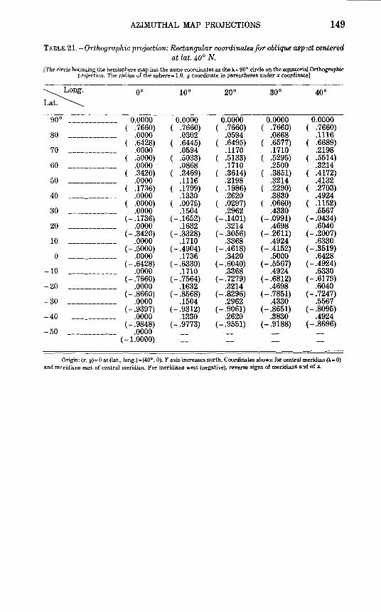
AZIMUTHAL MAP PROJECTIONS 149
TABLE 21. -Orthographic projection: Rectangular coordinates for oblique asp1ct centered at lat. 1,.0° N.
[The circle bounding the hemisphere mah has the same coordinates as the).= 90° circle on the equatorial Orthographic projection. The radius oft e sphere= 1.0. y coordinate in parentheses under x coordinate]
~ oo 100 20° 30° 40°
.
90° ------------ 0.0000 0.0000 0.0000 0.0000 0.0000 ( .7660) ( .7660) ( .7660) ( .7660) ( .7660)
80 ------------ .0000 .0302 .0594 .0868 .1116 .6428) .6445) .6495) .6577) .6689)
70 ------------ .0000 .0594 .1170 .1710 .2198 .5000) .5033) .5133) .5295) .5514)
60 ------------ .0000 .0868 .1710 .2500 .3214 .3420) .3469) .3614) .3851) .4172)
50 ------------ .0000 .1116 .2198 .3214 .4132 .1736) .1799) .1986) .2290) .2703)
40 ------------ .0000 .1330 .2620 .3830 .4924 .0000) .0075) .0297) .0660) .1152)
30 ------------ .0000 .1504 .2962 .4330 .5567 (- .1736) (- .1652) (- .1401) (- .0991) ( -.0434)
20 ------------ .0000 .1632 .3214 .4698 .6040 (- .3420) ( -.3328) ( -.3056) ( -.2611) ( -.2007)
10 ------------ .0000 .1710 .3368 .4924 .6330 (- .5000) (- .4904) ( -.4618) (- .4152) ( -.3519)
0 ------------ .0000 .1736 .3420 .5000 .6428 (- .6428) (- .6330) ( -.6040) ( -.5567) (- .4924)
-10 ------------ .0000 .1710 .3368 .4924 .6330 (- .7660) (- .7564) (- .7279) (-.6812) (- .6179)
-20 ------------ .0000 .1632 .3214 .4698 .6040 (- .8660) ( -.8568) ( -.8296) (- .7851) (- .7247)
-30 ------------ .0000 .1504 .2962 .4330 .5567 (- .9397) (- .9312) (- .9061) (- .8651) ( -.8095)
-40 ------------ .0000 .1330 .2620 .3830 .4924 ( -.9848) ( -.9773) ( -.9551) ( -.9188) ( -.8696)
-50 ------------ .0000 ( -1.0000)
Origin: (x, y)= 0 at (lat., long.) =(40°, 0). Y axis increases north. Coordinates shown for central meridian().= 0) and meridians east of central meridian. For meridians west (negative), reverse signs of meridians a"'l.d of x.
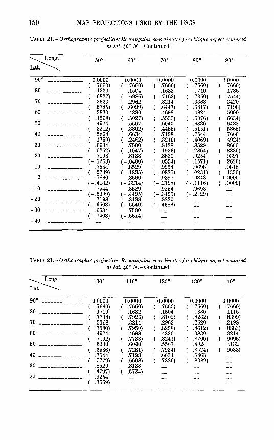
150 MAP PROJECTIONS USED BY THE USGS
TABLE 21. -Orthographic projection: Rectangular coordinates for nhlique aspPct centered at lat. 40° N. -Continued
~ 50° 60° 70° 80° 90° .
goo ------------ 0.0000 0.0000 0.0000 0.0000 0.0000 ( .7660) ( .7660) ( .7660) ( .7660) ( .7660)
80 ------------ .1330 .1504 .1632 .1710 .1736 .6827) .6986) ( .7162) ( .7350) .7544)
70 ------------ .2620 .2962 .3214 .3368 .3420
60 .5785) .6099) .6447) .6817) .7198)
------------ .3830 .4330 .4698 .4924 .5000 .4568) .5027) .5535) .6076) .6634)
50 ------------ .4924 .5567 .6040 .6330 .6428 .3212) .3802) .4455) .5151) .5868)
40 ------------ .5868 .6634 .7198 .7544 .7660 .1759) .2462) .3240) .4069) .4924)
30 ------------ .6634 .7500 .8138 .8529 .8660 .0252) .1047) .1926) .2864) .3830)
20 ------------ .7198 .8138 .8830 .9254 .9397 (- .1263) (- .0400) .0554) .1571) .2620)
10 ------------ .7544 .8529 .9254 .9698 .9848 (- .2739) (- .1835) (- .0835) .0231) ( .1330)
0 ------------ .7660 .8660 .9397 .9848 1.0000 {- .4132) {- .3214) (- .2198) (-.1116) ( .0000)
-10 ------------ .7544 .8529 .9254 .9698 (- .5399) (- .4495) (- .3495) (- .2429)
-20 ------------ .7198 .8138 .8830
-30 (- .6503) (- .5640) (- .4686)
------------ .6634 .7500 (- .7408) (- .6614)
-40 ------------
TABLE 21.-0rthographic projection: Rectangular coordinates for oblique a.spect centered at lat. 40° N. -Continued
~ 100° 110° 120° 130° 140° Lat.
90° -------------- 0.0000 0.0000 0.0000 0.0000 0.0000 ( .7660) ( .7660) ( .7660) ( .7660) ( .7660)
80 --------------- .1710 .1632 .1504 1330 .1116 .7738) .7926) ( .8102) .8262) ( .8399)
70 --------------- .3368 .3214 .2962 .2620 .2198 .7580) .7950) .8298) .8612) .8883)
60 --------------- .4924 .4698 .4330 .3830 .3214 .7192) .7733) .8241) .8700) .9096)
50 --------------- .6330 .6040 .5567 .4924 .4132 .6586) .7281) .7934) .Rf:i24) .9033)
40 --------------- .7544 .7198 .6634 f:i868 .5779) .6608) .7386) 8089)
30 --------------- .8529 .8138
20 ---------------.4797) .5734) .9254 .3669)
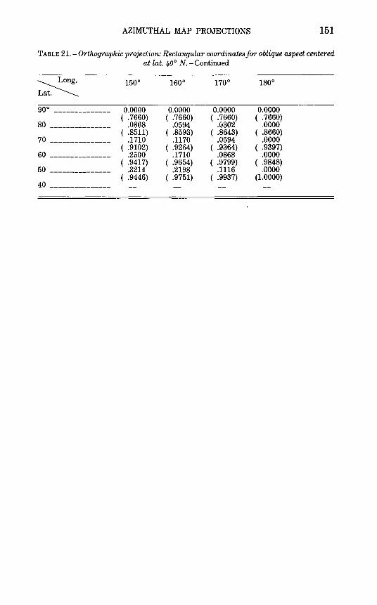
AZIMUTHAL MAP PROJECTIONS 151
TABLE 21.- Orthographic projection: Rectangular coordinates for oblique aspect centered at lat. 1,0° N. -Continued
~ 150° 160° 170° 180° .
90° -------------- 0.0000 0.0000 0.0000 0.0000 ( .7660) ( .7660) ( .7660) ( .7660)
80 --------------- .0868 .0594 .0302 .0000 ( .8511) ( .8593) ( .8643) ( .8660)
70 --------------- .1710 .1170 .0594 .0000 ( .9102) ( .9264) ( .9364) ( .9397)
60 --------------- .2500 .1710 .0868 .0000 ( .9417) ( .9654) ( .9799) ( .9848)
50 --------------- .3214 .2198 .1116 .0000
40 ---------------( .9446) ( .9751) ( .9937) (1.0000)

17. STEREOGRAPHIC PROJECTION
SUMMARY
• Azimuthal. • Conformal. • The central meridian and a particular parallel (if shown) are straight lir«!s. • All meridians on the polar aspect and the Equator on the equatorizl aspect are
straight lines. • All other meridians and parallels are shown as arcs of circles. • A perspective projection for the sphere. • Directions from the center of the projection are true (except on ellipsoidz I oblique and
equatorial aspects). • Scale increases away from the center of the projection. • Point opposite the center of the projection cannot be plotted. • Used for polar maps and miscellaneous special maps. • Apparently invented by Hipparchus (2nd century B.C.).
HISTORY
The Stereographic projection was probably known in its polar form to the Egyptians, while Hipparchus was apparently the firs~. Greek to use it. He is generally considered its inventor. Ptolemy referl""ed to it as "Planisphaerum," a name used into the 16th century. The name "Stereographic" was assigned to it by Fran~ois d' Aiguillon in 1613. The polar Stereographic was exclusively used for star maps untH perhaps 1507, when the earliest-known use for a map of the world w~-~ made by Walther Ludd (Gaultier Lud) of St. Die, Lorraine.
The oblique aspect was used by Theon of Alexandria in tr~ 4th century for maps of the sky, but it was not proposed for geograp'lical maps until Stabius and Werner discussed it together with their cordiform (heart-shaped) projections in the early 16th century. Th~ earliestknown world maps were included in a 1583 atlas by Jacques de Vaulx (c. 1555-97). The two hemispheres were centered on Paris and its opposite point, respectively.
The equatorial Stereographic originated with the Arabs,, and was used by the Arab astronomer Ibn-el-Zarkali (1029-87) of Tohdo for an astrolabe. It became a basis for world maps in the early 16th century, with the earliest known examples by Jean Roze (or Rotz}, a 1' lorman, in 1542. After Rumold (the son of Gerhardus) Mercator's nse of the equatorial Stereographic for the world maps of the atlas of 1595, it became very popular among cartographers (Keuning, 195Fi, p. 7-9; Nordenskiold, 1889, p. 90, 92-93).
153
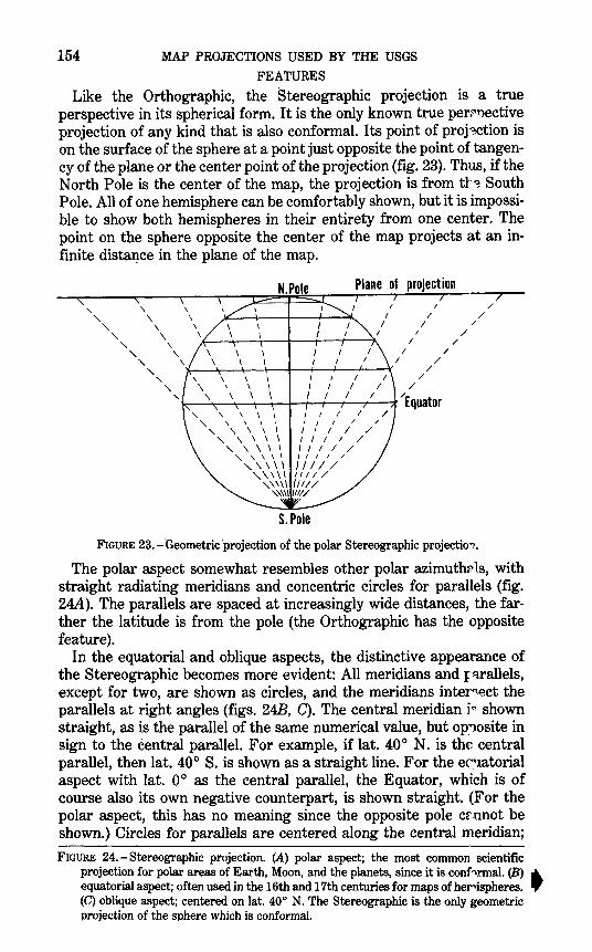
154 MAP PROJECTIONS USED BY THE USGS
FEATURES
Like the Orthographic, the S tereographic projection is a true perspective in its spherical form. It is the only known true per;;"Dective projection of any kind that is also conformal. Its point of proj<'?.ction is on the surface of the sphere at a point just opposite the point of tangency of the plane or the center point of the projection (fig. 23). Thus, if the North Pole is the center of the map, the projection is from tl'·'?. South Pole. All of one hemisphere can be comfortably shown, but it is impossible to show both hemispheres in their entirety from one center. The point on the sphere opposite the center of the map projects at an infinite distance in the plane of the map.
' " " ' ' " ' ' ' ' '~~~+-~~~~~-r~---*
S.Pole
FIGURE 23.-Geometric ·projection of the polar Stereographic projectio,-.
The polar aspect somewhat resembles other polar azimuthrls, with straight radiating meridians and concentric circles for parallels (fig. 24A). The parallels are spaced at increasingly wide distances, the farther the latitude is from the pole (the Orthographic has the opposite feature).
In the equatorial and oblique aspects, the distinctive appearance of the Stereographic becomes more evident: All meridians and rvallels, except for two, are shown as circles, and the meridians inter"~ct the parallels at right angles (figs. 24B, C). The central meridian i~ shown straight, as is the parallel of the same numerical value, but opposite in sign to the central parallel. For example, if lat. 40° N. is the central parallel, then lat. 40° S. is shown as a straight line. For the ec'Iatorial aspect with lat. 0° as the central parallel, the Equator, which is of course also its own negative counterpart, is shown straight. (For the polar aspect, this has no meaning since the opposite pole cr.nnot be shown.) Circles for parallels are centered along the central meridian;
FIGURE 24.- Stereographic projection. (A) polar aspect; the most common scientific projection for polar areas of Earth, Moon, and the planets, since it is conf'lrmal. (B) A. equatorial aspect; often used in the 16th and 17th centuries for maps of hel"'ispheres. .,(C) oblique aspect; centered on lat. 40° N. The Stereographic is the only geometric projection of the sphere which is conformal.
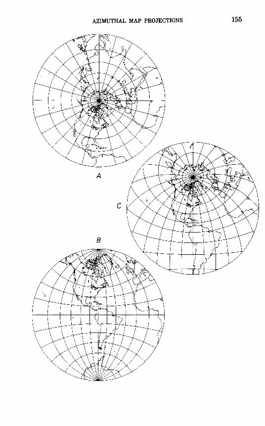
AZIMUTHAL MAP PROJECTIONS 155
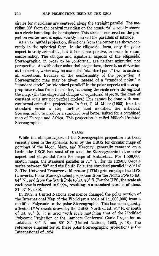
156 MAP PROJECTIONS USED BY THE USGS
circles for meridians are centered along the straight parallel. The meridian 90° from the central meridian on the equatorial aspect i~ shown as a circle bounding the hemisphere. This circle is centered on the projection center and is equidistantly marked for parallels of latitude.
As an azimuthal projection, directions from the center are shown correctly in the spherical form. In the ellipsoidal form, only tl:~ polar aspect is truly azimuthal, but it is not perspective, in order to retain conformality. The oblique and equatorial aspects of the ellipsoidal Stereographic, in order to be conformal, are neither azimuthal nor perspective. As with other azimuthal projections, there is no di<:'t.ortion at the center, which may be made the "standard point" true to scale in all directions. Because of the conformality of the projection, a Stereographic map may be given, instead of a "standard :point," a "standard circle" (or "standard parallel" in the polar aspect) with an appropriate radius from the center, balancing the scale error thr~1ughout the map. (On the ellipsoidal oblique or equatorial aspects, the lines of constant scale are not perfect circles.) This cannot be done with nonconformal azimuthal projections. In fact, 0. M. Miller (1953) took the standard circle a step further and modified the s:...,herical Stereographic to produce a standard oval better suited for a combined map of Europe and Africa. This projection is called Miller's Prolated Stereographic.
USAGE
While the oblique aspect of the Stereographic projection 11 as been recently used in the spherical form by the USGS for circular maps of portions of the Moon, Mars, and Mercury, generally center~d on a basin, the USGS has most often used the Stereographic in the polar aspect and ellipsoidal form for maps of Antarctica. For 1:500,000 sketch maps, the standard parallel is 71° S.; for its 1:250,0l)0-scale series between 80° and the South Pole, the standard parallel i~ 80°14' S. The Universal Transverse Mercator (UTM) grid employs the UPS (Universal Polar Stereographic) projection from the North Po~e to lat. 84 ° N., and from the South Pole to lat. 80° S. For the UPS, the scale at each pole is reduced to 0.994, resulting in a standard parallel of about 81 °07' N. or S.
In 1962, a United Nations conference changed the polar pC'..-tion of the International Map of the World (at a scale of 1:1,000,000) from a modified Polyconic to the polar Stereographic. This has consequently affected IMW sheets drawn by the USGS. North of lat. 84 oN. or south of lat. 80° S., it is used "with scale matching that of the I"odified Polyconic Projection or the Lambert Conformal Conic Projection at Latitudes 84 ° N. and 80° S." (United Nations, 1963, p. lO). The reference ellipsoid for all these polar Stereographic projections is the International of 1924.
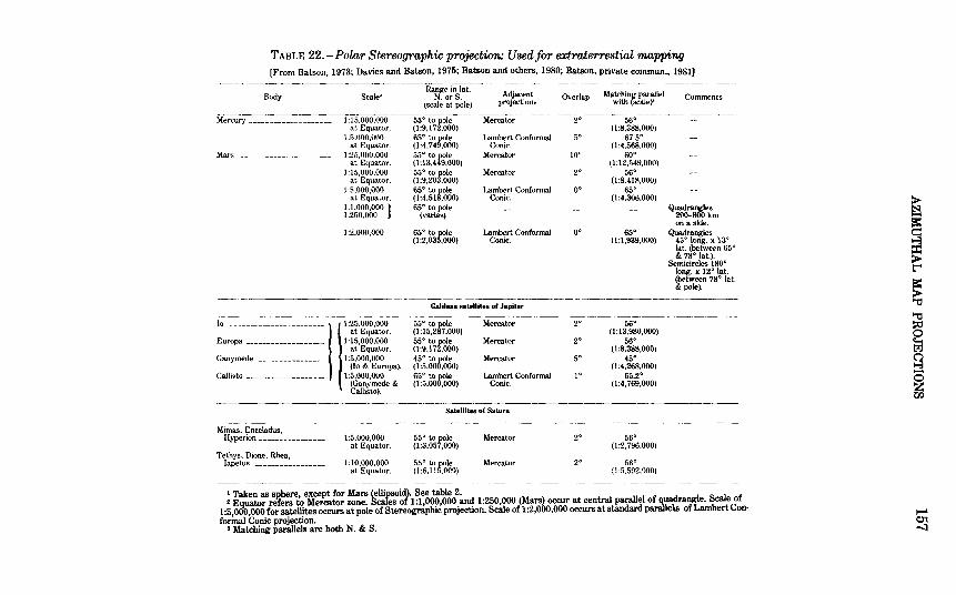
TABLE 22.-Polar Stereographic projection: Usedfor extraterrestial mapping [From Batson, 1973; Davies and Batson, 1975; Batson and others, 1980; Batson, private commun., 1981]
---------------------- ----Range in hiL-Body' Scale' N. or S.
(scale at pole) AdJacent
proJections Overlap Ma~t~nfslJ!~Iel Comments
Mercury -------------------- 1:15,000,000 55° to r.t,le Mercator --y----5so------------
at Equator (1:9,17 ,000) (1:8,388,000) 1:5,000,000 r1~~-~~rJ&) LambE-rt Conformal 5. 67.5°
at Equator. Conic. (1:4,568,000) Mars----------------------- 1:25,000,000 f1~ ~iA!9.'00o> Mercator to• so•
at Equator. (1:12,549,000) 1:15,000,000 f1~;JofJJoo) Mercator 20 56°
at Equator. (1:8,418,000) 1·5,000,000 r1~~-~~00) Lambert Conformal o• 65°
at Equator. Conic. ( 1 :4,306,000) 1:1,000,000 } 65° to pole -- -- -- ~r:_a~e~m 1:250,000 (varies)
on a side. 1:2,000.000 r1~;}:3rdoo, Lambert Conformal o• 65° Quadrangles
Conic. (1:1,939,000) 45° long. x 13° lat. (betwet>n 65° & 78° lat.).
Semicircles 180° long. x 12° lat. (between 78° lat & pole).
---- -------------------------~~-------Galilean satellites of Jupiter ----------------------------
lo ----------------------- rffi~.~ r1~~i.~&?.looo) Mercator 20 56°
at Equator. (1:13,980,000) Europa ------------------- 1:15,000,000 ff~.~~r.doo) Mercator 20 56°
at Equator. (1:8,388,000) Ganymede ---------------- 1:5,000,000 f1~~-~~f.doo) Mercator 5• 45°
(lo & Europa). (1:4,268,000) Callisto ------------------- 1:5,000,000 rf~.~~r.doo) Lambert Conformal 10 65.2°
(Ganymede & Conic. (1:4,769,000) Callisto).
Satellites of Saturn
Mimas, Enceladus, Hyperion ---------------- 1:5,000,000 f1~;-~~r.'doo) Mercator 20 56°
at Equator. ( 1:2, 796,000) Tethys, Dione, Rhea,
Iapetus ----------------- 1:10,000,000 r~~;j~f.O'~o) Mercator 20 56° at Equator. (1:5,592,000)
1 Taken as s~here, except for Mars (ellipsoid). See table 2. z Equator refers to Mercator zone. Scales of 1:1,000,000 and 1:250,000 (Mars) occur at central parallel of qlladrangle. Scale of
1:5,000,000 for satellites occurs at pole of Stereographic projection. Scale of 1:2,000,000 occurs at standard paralle1.s of Lambert Conformal Conic projection.
a Matching pariillels are both N. & S.
> IS -rs: ~
~ > t"'
a:: > '"1:1 '"1:1
~ t;j 0 t-3 -0 z 00
1-1 01 -:t
158 MAP PROJECTIONS USED BY THE USGS
~he Astrogeology Center of the Geological Survey at Flagstaff, Ar1z., has been using the polar Stereographic for the mapping· of polar areas of Mars, Mercury, and satellites of Jupiter and Saturn at various scales (see table 22).
The USGS is preparing a geologic map of the Arctic regions, using as a base an American Geographical Society map of the Arctic at a scale of 1:5,000,000. Drawn to the Stereographic projection, th~ map is based on a sphere having a radius which gives it the same volume as the International ellipsoid, and lat. 71 o N. is made the standard parallel.
FORMULAS FOR THE SPHERE
Mathematically, a point at a given angular distance from tl'~ chosen center point on the sphere is plotted on the Stereographic :projection at a distance from the center proportional to the trigonometric tangent of half that angular distance, and at its true. azimuth, or, if the central scale factor is 1,
p = 2R tan 1f2 c 8= r-Az= 180° -Az k= sec2112 c
(17-1) (16-2)
(17-1a)
where cis the angular distance from the center, Az is the azirnuth east of north (see equations (5-3) through (5-6)), and (} is the pc lar coordinate east of south. Combining with standard equations, the formulas for rectangular coordinates of the oblique Stereographic proje~tion are found to be as follows, given R, k0 , cPIJ Ao, c/>, and A:
x = Rk cos cJ> sin (A- Ao) y = Rk [cos c/>1 sin c1>- sin c/>1 cos c1> cos (A- Ao)]
where
k = 2kof[1 +sin cPt sin cJ> +cos c/>1 cos cJ> cos (A- Ao)]
(17-2) (17-3)
(17-4)
and ( cPtJ Ao) are the latitude and longitude of the center, which is also the origin. Since this is a conformal projection, k is the scale factor in all directions, based on a central scale factor of k0 , normally 1.0, r•1t which may be reduced. The Y axis coincides with the central meridian Ao, y increasing northerly and x, easterly.
If cJ> = - c/> 0 and A= Ao ± 180°, the point cannot be plotted. Geo"lletrically, it is the point from which projection takes place.
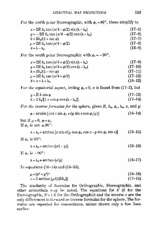
AZIMUTHAL MAP PROJECTIONS 159
For the north polar Stereographic, with c/> 1 = 90°, these simplify to
x = 2R k0 tan ( 1r/4- cj>/2) sin(>-.- Ao) y = - 2R ko tan ( rr/4- cj>/2) cos (A- >-.o) k = 2k0/(1 + sin cf>) p = 2R k0 tan ( 1rl4- cj>/2) O=A-Ao
For the south polar Stereographic with cf>, = -90°,
x = 2R k0 tan ( 1r/4 + cj>/2) sin(>-.- Ao) y = 2R k0 tan ( 1r/4 + cj>/2) cos(>-.- Ao) k = 2k0/(1- sin cf>) p = 2R k0 tan (7r/4 + cp/2) 0=7r-A+Ao
(17-5) (17-6) (17-7) (17-8) (16-9)
(17-9) (17-10) (17-11) (17-12) (16-12)
For the equatorial aspect, letting c/> 1 = 0, xis found from (17-2), but
y =R k sin cf> (17-13) k = 2 k0/[1 +COS cf> COS (A- Ao)] (17-14)
Fo-r the inverse fo·nnulas for the sphere, given R, k0 , c/> 11 A0 , x, and y:
cp =arcsin [cos c sin cf>, + (y sin c cos cf> 1/ p )]
but if p=O, cf>=cf> 1 •
If </J 1 is not ±90°:
A= Ao+ arctan [x sin c/(p cos cf> 1 cos c-y sin c/> 1 sin c)]
If c/> 1 is 90°:
A= Ao +arctan [x/(- y)]
If </J 1 is -90°:
A= Ao +arctan (xly)
In equations (16-14) and (16-15),
P = (x2 + y2y12 c = 2 arctan lp/(2Rko)]
(16-14)
(16-15)
(16-16)
(16-17)
(16-18) (17-15)
The similarity of formulas for Orthographic, Stereographic, and other azimuthals n1ay be noted. The equations for It (k for the Stereographic, It= 1.0 for the Orthographic) and the inverse care the only differences in forward or inverse formulas for the sphere. The formulas are repeated for convenience, unless shown only a few lines earlier.
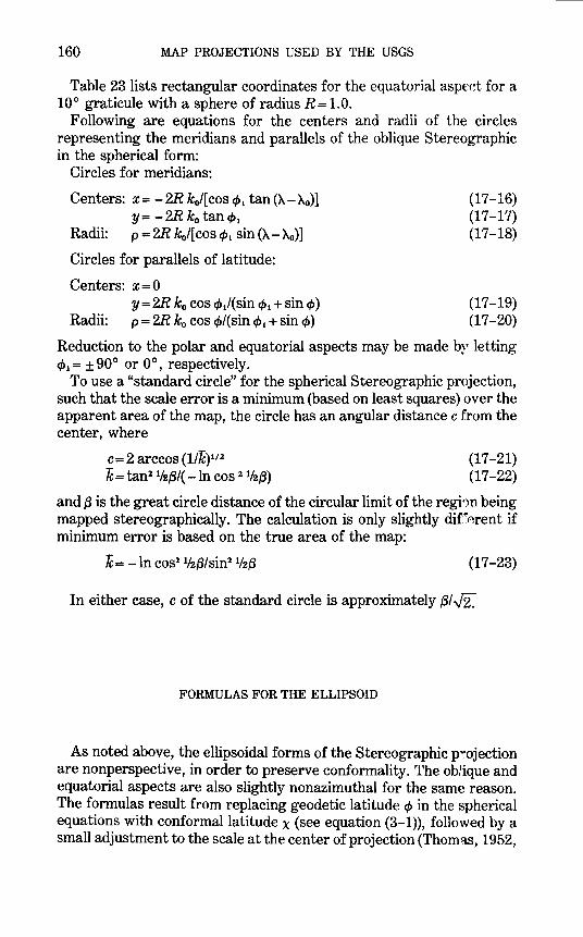
160 MAP PROJECTIONS USED BY THE USGS
Table 23 lists rectangular coordinates for the equatorial aspe~t for a 10° graticule with a sphere of radius R= 1.0.
Following are equations for the centers and radii of the circles representing the meridians and parallels of the oblique Stereographic in the spherical form:
Circles for meridians:
Centers: x = - 2R kof[ cos c/>1 tan(>.- >.o)] Y= -2R ko tan c/>1
Radii: p = 2R k0 /[ cos c/>1 sin(>.- >.o)]
Circles for parallels of latitude:
Centers: x = 0 y=2R k0 cos cp1/(sin c/>1 +sin cp)
Radii: p = 2R k0 cos ¢/(sin c/>1 +sin cJ>)
(17-16) (17-17) (17-18)
(17-19} (17-20)
Reduction to the polar and equatorial aspects may be made b~r letting c/>1 = ± 90° or 0°, respectively.
To use a "standard circle" for the spherical Stereographic projection, such that the scale error is a minimum (based on least squares) over the apparent area of the map, the circle has an angular distance c from the center, where
c = 2 arccos (1/k)112
k = tan2 1/2(3/( -ln cos 2 112(3) (17-21) (17-22)
and (3 is the great circle distance of the circular limit of the regi')n being mapped stereographically. The calculation is only slightly dif'!'~~rent if minimum error is based on the true area of the map:
(17-23)
In either case, c of the standard circle is approximately (315,
FORMULAS FOR THE ELLIPSOID
As noted above, the ellipsoidal forms of the Stereographic p•ojection are nonperspective, in order to preserve conformality. The obHque and equatorial aspects are also slightly nonazimuthal for the same reason. The formulas result from replacing geodetic latitude cJ> in the spherical equations with conformal latitude x (see equation (3-1)), followed by a small adjustment to the scale at the center of projection (Thom::ts, 1952,
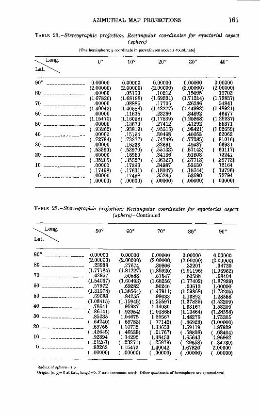
AZIMUTHAL MAP PROJECTIONS 161
TABLE 23. -Stereographic projection: Rectangular coordinates for equa,torial aspect (sphere)
[One hemisphere; y coordinate in parentheses under x coordinate]
~ oo 100 20° 30° 40°
.
90° -------------- 0.00000 0.00000 0.00000 0.00000 0.00000 (2.00000) (2.00000) (2.00000) (2.00000) (2.00000)
80 --------------- .00000 .05150 .10212 .15095 .19703 (1.67820) (1.68198) (1.69331) (1.71214) (1.73837)
70 --------------- .00000 .08885 .17705 .26386 .34841 (1.40042) (1.40586) (1.42227) (1.44992) (1.48921)
60 --------------- .00000 .11635 .23269 .34892 .46477 (1.15470) (1.16058) (1.17839) (1.20868) (1.25237)
50 --------------- .00000 .13670 .27412 .41292 .55371 ( .93262) ( .93819) ( .95515) ( .98421) (1.02659)
40 --------------- .00000 .15164 .30468 .46053 .62062 ( .72794) ( .73277) ( .74749) ( .77285) ( .81016)
30 --------------- .00000 .16233 .32661 .49487 .66931 ( .53590) ( .53970) ( .55133) ( .57143) ( .60117)
20 --------------- .00000 .16950 .34136 .51808 .70241 { .35265) ( .35527) ( .36327) ( .37713) ( .39773)
10 --------------- .00000 .17363 .34987 .53150 .72164 ( .17498) ( .17631) ( .18037) ( .18744) ( .19796)
0 --------------- .00000 .17498 .35265 .53590 .72794 ( .00000) ( .00000) ( .00000) ( .00000) ( .00000)
TABLE 23.-Stereographic projection: Rectangular coordinates for eq'UC'torial aspect (sphere)- Continued
~ 50° 60° 70° 80° 90° .
90° -------------- 0.00000 0.00000 0.00000 0.00000 0.00000
80 ---------------(2.00000) (2.00000) (2.00000) (2.00000) (2.00000)
.23933 .27674 .30806 .33201 .34730
70 ---------------(1.77184) (1.81227) (1.85920) (1.91196) (1.96962)
.42957 .50588 .57547 .63588 .68404
60 ---------------(1.54067) (1.60493) (1.68256) (1.77402) (1.87939)
.57972 .69282 .80246 .90613 1.00000
50 ---------------(1.31078) (1.38564) (1.47911) (1.59368) (1.73205)
.69688 .84255 .99033 1.13892 1.28558
40 ---------------(1.08415) (1.15945) (1.25597) (1.37825) (1.53209)
.78641 .95937 1.14080 1.33167 1.53209
30 ---------------( .86141) ( .92954) (1.01868) (1.13464) (1.28558)
.85235 1.04675 1.25567 1.48275 1.73205
20 ---------------( .64240) ( .69783) ( .77149) ( .86928) (1.00000)
.89755 1.10732 1.33650 1.59119 1.87939
10 ---------------( .42645) ( .46538) ( .51767) ( .58808) ( .68404)
.92394 1.14295 1.38450 1.65643 1.96962
0 ---------------( .21267) ( .23271) ( .25979) ( .29658) ( .34730)
.93262 1.15470 1.40042 1.67820 2.00000 ( .00000) ( .00000) ( .00000) ( .00000) ( .00000)
Radius of sphere= 1.0. Origin: (x, y)=O at (lat., long.)=O. Y axis increases north. Other quadrants of hemisphere are symmetrical.
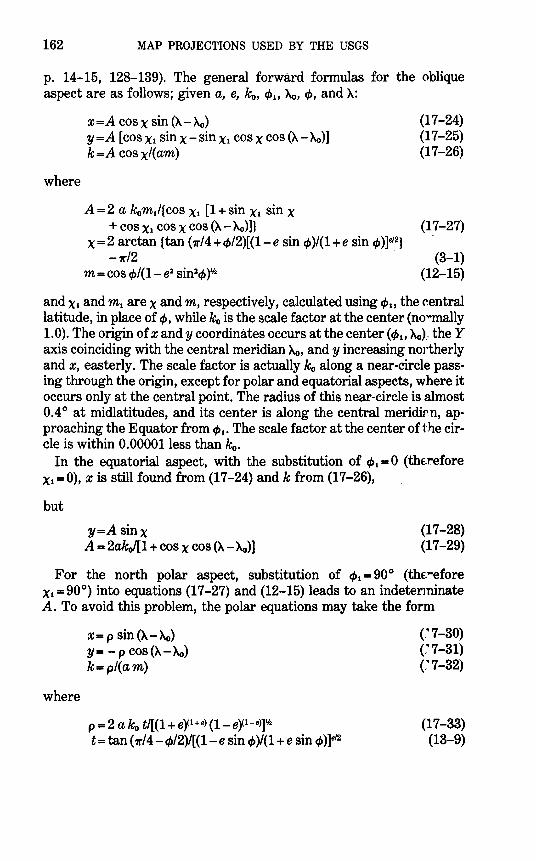
162 MAP PROJECTIONS USED BY THE USGS
p. 14-15, 128-139). The general forward formulas for the oblique aspect are as follows; given a, e, k0 , t/>11 ~' q,, and A:
where
x =A cos x sin (A-~) y=A [cos Xt sin x-sin X1 cos x cos (A-~)] k=A cosxl(am)
A= 2 a komt/{ cos Xt [1 +sin Xt sin x + cos X1 cos X cos (A-~)]}
x=2 arctan {tan (7r/4+tj>/2)[(1-e sin q,)/(1+e sin q,)]ei2J -11"/2
m =cos q,/(1- e2 sin2tf> y12
(17-24) (17-25) (17-26)
(17-27)
(3-1) (12-15)
and Xt and m1 are x and m, respectively, calculated using tf>t, the central latitude, in place of q,, while ko is the scale factor at the center (no~ally 1.0). The origin of x andy coordinates occurs at the center (t/>11 ~) .. the Y axis coinciding with the central meridian ~' and y increasing northerly and x, easterly. The scale factor is actually ko along a near-circle passing through the origin, except for polar and equatorial aspects, where it occurs only at the central point. The radius of this near-circle is almost 0.4 ° at midlatitudes, and its center is along the central meridirm, approaching the Equator from t/> 1 • The scale factor at the center of the circle is within 0.00001less than ko.
In the equatorial aspect, with the substitution of tf>t = 0 (thE.refore Xt = 0), x is still found from (17-24) and k from (17-26),
but
y=A sinx A= 2ako/[1 +cos x cos (A-~)]
(17-28) (17-29)
For the north polar aspect, substitution of t/> 1 = 90° (the,..efore X1 = 90°) into equations (17 -27) and (12-15) leads to an indeter1ninate A. To avoid this problem, the polar equations may take the form
where
X= p sin(A-~) Y= -p COS(A-~) k= pi( am)
p = 2 a k0 t/[(1 + e~lu) (1- e~l-e)Jh
t= tan (11"/4- q,/2)/[(1- e sin q,)/(1 +e sin t/>)]612
C7-30) (J 7-31) C7-32)
(17-33) (13-9)
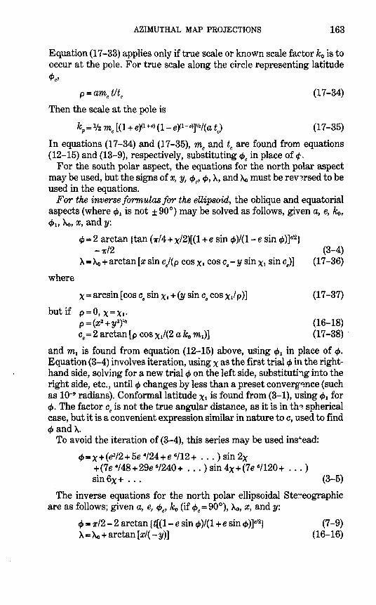
AZIMUTHAL MAP PROJECTIONS 163
Equation (17 -33) applies only if true scale or known scale factor k0 is to occur at the pole. For true scale along the circle representing latitude
cPc' p =amc t!tc (17-34)
Then the scale at the pole is
kp = 1/2 me [(1 + eY1 +e> (1- eY1-e>J12I(a tc) (17-35)
In equations (17 -34) and (17 -35), me and tc are found from equations (12-15) and (13-9), respectively, substituting cl>c in place of¢.
For the south polar aspect, the equations for the north polar aspect may be used, but the signs of x, y, cl>c' cJ>, A, and Ao must be rev,.~rsed to be used in the equations.
For the inverse formulas for the ellipsoid, the oblique and equatorial aspects (where c/>1 is not ± 90°) may be solved as follows, given a, e, ko, ¢., Ao, x, and y:
where
¢=2 arctan [tan (?rl4+x/2)[(1+e sin ¢)/(1-e sin c/>)]e12}
-?r/2 A= Ao+ arctan [x sin cj(p cos X1 cos ce -y sin X1 sin C
8)]
x= arcsin [cos C8 sin Xt +(y sin C8 cos Xt/p)]
but if p=O, x=x1· P = (x:z + y:z)lh C8= 2 arctan [p cos Xt/(2 a k0 m1)]
(3-4) (17-36)
(17-37)
(16-18) (17-38)
and m1 is found from equation (12-15) above, using ¢ 1 in place of¢. Equation (3-4) involves iteration, using x as the first trial cJ> in the righthand side, solving for a new trial cJ> on the left side, substituti1.g into the right side, etc., until cJ> changes by less than a preset converg-~nce (such as 10-9 radians). Conformal latitude X1 is found from (3-1), using c/>1 for cJ>. The factor ce is not the true angular distance, as it is in tha. spherical case, but it is a convenient expression similar in nature to c, used to find c1> and}...
To avoid the iteration of (3-4), this series may be used ins~ead:
c/>=x+(e212+5e 4/24+e 6/12+ ... ) sin 2x +(7e 4/48+29e 6/240+ ... ) sin 4x+(7e 6/120+ ... ) sin 6x + . . . (3-5)
The inverse equations for the north polar ellipsoidal Ste:--eographic are as follows; given a, e, cl>c' ko (if cl>c = 90°), Ao, x, and y:
c1> = 1r/2- 2 arctan {t[(1- e sin ¢)/(1 + e sin ¢)]812}
A=Ao+arctan [x/( -y)] (7-9)
(16-16)
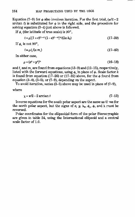
164 MAP PROJECTIONS USED BY THE USGS
Equation (7 -9) for cp also involves iteration. For the first trial, ( 1r/2- 2 arctan t) is substituted for cp in the right side, and the procedure for solving equation (3-4) just above is followed.
If cf>c (the latitude of true scale) is 90°,
t= p[(1 +e~l+e) (1-e~l-e>J12/(2a ko) (17-39)
If cf>c is not 90°,
t=pt/(amc)
In either case,
P =(x2+yl)lf2
(17-40)
(16-18)
and tc and me are found from equations (13-9) and (12-15), respe~tively, listed with the forward equations, using cf>c in place of cp. Scale factor k is found from equation (17-26) or (17-32) above, for the cp fouiJd from equation (3-4), (3-5), or (7 -9), depending on the aspect.
To avoid iteration, series (3-5) above may be used in place of (7 -9),
where
x = 1r/2- 2 arctan t (7-13)
Inverse equations for the south polar aspect are the same as tl' 'lSe for the north polar aspect, but the signs of x, y, Xo, cf>c, cp, and A nust be reversed.
Polar coordinates for the ellipsoidal form of the polar Stereosraphic are given in table 24, using the International ellipsoid and a central scale factor of 1.0.
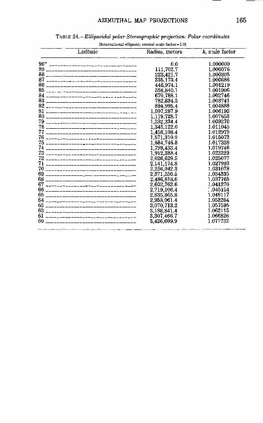
AZIMUTHAL MAP PROJECTIONS
TABLE 24.-Ellipsoidal polar Stereographic projection: Polar coo'rdinates (International ellipsoid; central scale factor= 1.0)
Latitude Radius, meters
90° -------------------------------89 _______________________________ _ 88 _______________________________ _
87 --------------------------------86 _______________________________ _ 85 _______________________________ _ 84 _______________________________ _ 83 _______________________________ _ 82 _______________________________ _ 81 _______________________________ _ 80 _______________________________ _ 79 _______________________________ _ 78 _______________________________ _
77 --------------------------------76 _______________________________ _ 75 _______________________________ _
74 --------------------------------73 --------------------------------72 --------------------------------71 --------------------------------70 _______________________________ _ 69 _______________________________ _ 68 _______________________________ _
67 ------------------------------~-66 _______________________________ _ 65 _______________________________ _ 64 _______________________________ _ 63 _______________________________ _ 62 _______________________________ _
61 --------------------------------60 _______________________________ _
0.0 111,702.7 223,421.7 335,173.4 446,974.1 558,840.1 670,788.1 782,834.3 894,995.4
1,007,287.9 1,119,728.7 1,232,334.4 1,345,122.0 1,458,108.4 1,571,310.9 1,684,746.8 1, 798,433.4 1,912,388.4 2,026,629.5 2,141,174.8 2,256,042.3 2,371,250.5 2,486,818.0 2,602,763.6 2, 719,106.4 2,835,865.8 2,953,061.4 3,070, 713.2 3,188,841.4 3,307,466.7 3,426,609.9
k, s<~ale factor
1.000000 1.000076 1.000305 1.000686 1.001219 1.001906 1.002746 1.003741 1.004889 1.006193 1.007653 1.009270 1.011045 1.012979 1.015073 1.017328 1.019746 1.022329 1.025077 1.027993 1.031078 1.034335 1.037765 1.041370 1.045154 1.049117 1.053264 1.057595 1.062115 1.066826 1.071732
165

18. LAMBERT AZIMUTHAL EQUAL-AREA PROJECTI9N
SUMMARY
• Azimuthal. • Equal-Area. • All meridians in the polar aspect, the central meridian in other arnects, and the
Equator in the equatorial aspect are straight lines. • The outer meridian of a hemisphere in the equatorial aspect (for the sphere) and the
parallels in the polar aspect (sphere or ellipsoid) are circles. • All other meridians and parallels are complex curves. • Not a perspective projection. • Scale decreases radially as the distance increases from the center, the only point with
out distortion. • Scale increases in the direction perpendicular to radii as the distance increases from
the center. • Directions from the center are true for the sphere and the polar ellipmidal forms. • Point opposite the center is shown as a circle surrounding the map (fer the sphere). • Used for maps of continents and hemispheres. • Presented by Lambert in 1772.
HISTORY
The last major projection presented by Johann Heinrich Lambert in his 1772 Beitrage was his azimuthal equal-area projectio'1 (Lambert, 1772, p. 75-78). His name is usually applied to the projecticn in modern references, but it is occasionally called merely the Ar.imuthal (or Zenithal) Equal-Area projection. Not only is it equal-ar~a, with, of course, the azimuthal property showing true directions from the center of the projection, but its scale at a given distance from the c~nter varies less from the scale at the center than the scale of any of the other major azimuthals (see table 19).
Lambert discussed the polar and equatorial aspects of th~ Azimuthal Equal-Area projection, but the oblique aspect is just as p'lpular now. The polar aspect was apparently independently derived by De Lorgna in Italy in 1789, and the latter was called the originator in a publication a century later (USC&GS, 1882, p. 290). G. A. Ginsburg p:--oposed two modifications of the general Lambert Azimuthal projectio'1 in 1949 to reduce the angular distortion at the expense of creating a flight distortion in area (Maling, 1960, p. 206).
FEATURES
The Lambert Azimuthal Equal-Area projection is not a perspective projection. It may be called a "synthetic" azimuthal in thr.t it was derived for the specific purpose of maintaining equal area. Tr~ ellipsoidal
167
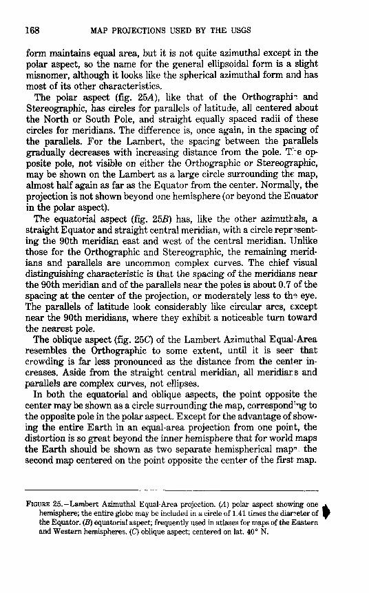
168 MAP PROJECTIONS USED BY THE USGS
form maintains equal area, but it is not quite azimuthal except in the polar aspect, so the name for the general ellipsoidal form is a slight misnomer, although it looks like the spherical azimuthal form and has most of its other characteristics.
The polar aspect (fig. 25A), like that of the Orthographh and Stereographic, has circles for parallels of latitude, all centered about the North or South Pole, and straight equally spaced radii of these circles for meridians. The difference is, once again, in the spacing of the parallels. For the Lambert, the spacing between the parallels gradually decreases with increasing distance from the pole. Tf~e opposite pole, not visible on either the Orthographic or Stereographic, may be shown on the Lambert as a large circle surrounding thE: map, almost half again as far as the Equator from the center. Normally, the projection is not shown beyond one hemisphere (or beyond the Eouator in the polar aspect).
The equatorial aspect (fig. 25B) has, like the other azimutllals, a straight Equator and straight central meridian, with a circle repr~senting the 90th meridian east and west of the central meridian. Unlike those for the Orthographic and Stereographic, the remaining meridians and parallels are uncommon complex curves. The chief visual distinguishing characteristic is that the spacing of the meridians near the 90th meridian and of the parallels near the poles is about 0. 7 of the spacing at .the center of the projection, or moderately less to tha. eye. The parallels of latitude look considerably like circular arcs, E:xcept near the 90th meridians, where they exhibit a noticeable turn toward the nearest pole.
The oblique aspect (fig. 25C) of the Lambert Azimuthal Equal-Area resembles the Orthographic to some extent, until it is seer that crowding is far less pronounced as the distance from the center increases. Aside from the straight central meridian, all meridians and parallels are complex curves, not ellipses.
In both the equatorial and oblique aspects, the point opposite the center may be shown as a circle surrounding the map, correspond~"'lg to the opposite pole in the polar aspect. Except for the advantage of showing the entire Earth in an equal-area projection from one point, the distortion is so great beyond the inner hemisphere that for world maps the Earth should be shown as two separate hemispherical map~, the second map centered on the point opposite the center of the first map.
FIGURE 25.- Lambert Azimuthal Equal-Area projection. (A) polar aspect showing one &. hemisphere; the entire globe may be included in a circle of 1.41 times the dianeter of ~ the Equator. (B) equatorial aspect; frequently used in atlases for maps of the Eastern and Western hemispheres. (C) oblique aspect; centered on lat. 40° N.
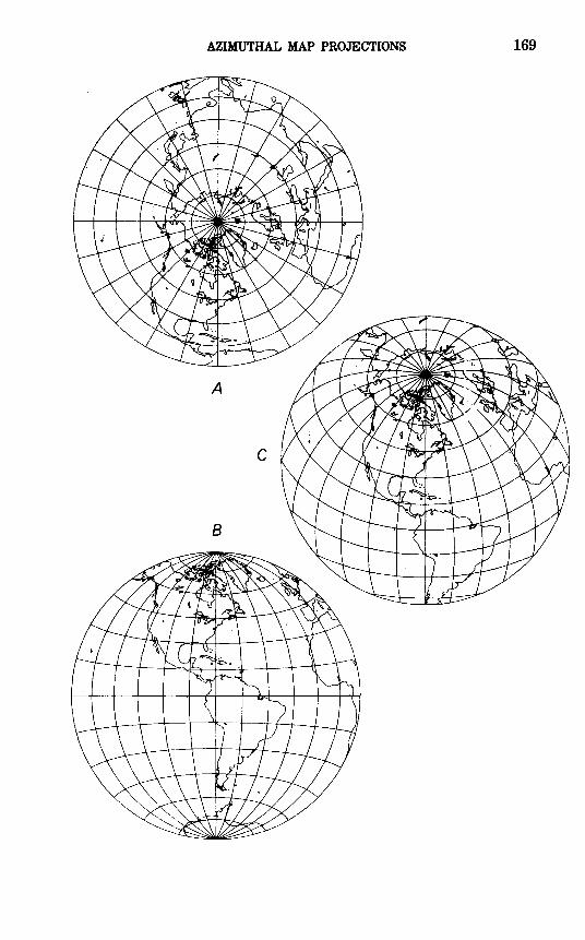
AZIMUTHAL MAP PROJECTIONS 169
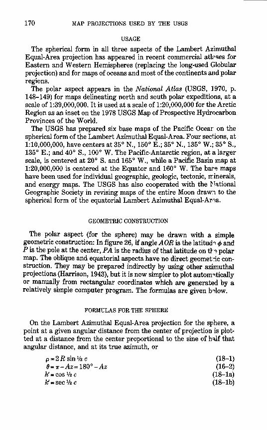
170 MAP PROJECTIONS USED BY THE USGS
USAGE
The spherical form in all three aspects of the Lambert Azimuthal Equal-Area projection has appeared in recent commercial atlrses for Eastern and Western Hemispheres (replacing the long-used Globular projection) and for maps of oceans and most of the continents and polar regions.
The polar aspect appears in the National Atlas (USGS, 1970, p. 148-149) for maps delineating north and south polar expeditions, at a scale of 1:39,000,000. It is used at a scale of 1:20,000,000 for the Arctic Region as an inset on the 1978 USGS Map of Prospective Hydrocarbon Provinces of the World.
The USGS has prepared six base maps of the Pacific Ocear on the spherical form of the Lambert Azimuthal Equal-Area. Four sections, at 1:10,000,000, have centers at 35° N., 150° E.; 35° N., 135° W.; 35° S., 135° E.; and 40° S., 100° W. The Pacific-Antarctic region, at a larger scale, is centered at 20° S. and 165° W., while a Pacific Basin map at 1:20,000,000 is centered at the Equator and 160° W. The bar~ maps have been used for individual geographic, geologic, tectonic, minerals, and energy maps. The USGS has also cooperated with the National Geographic Society in revising maps of the entire Moon draw:~ to the spherical form of the equatorial Lambert Azimuthal Equal-Ar,.~a.
GEOMETRIC CONSTRUCTION
The polar aspect (for the sphere) may be drawn with a simple geometric construction: In figure 26, if angle AOR is the latitud~ cp and P is the pole at the center, PA is the radius of that latitude on tl' ~ polar map. The oblique and equatorial aspects have no direct geometic construction. They may be prepared indirectly by using other azimuthal projections (Harrison, 1943), but it is now simpler to plot autom-:~.tically or manually from rectangular coordinates which are generated by a relatively simple computer program. The formulas are given b~low.
FORMULAS FOR THE SPHERE
On the Lambert Azimuthal Equal-Area projection for the sphere, a point at a given angular distance from the center of projection is plotted at a distance from the center proportional to the sine of half that angular distance, and at its true azimuth, or
p =2R sin 1/2 c 8= 1r-Az= 180° -Az h'= cos 112 c It= sec 112 c
(18-1) (16-2)
(18-1a) (18-1b)
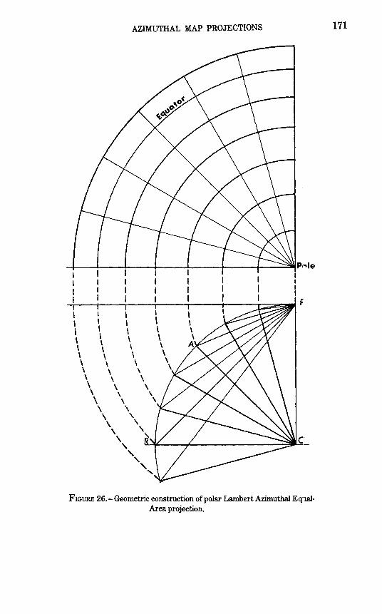
l
' \ \ \ \ \ \ \
I
' ' \ \ \ \ \ \ \
AZIMUTHAL MAP PROJECTIONS
I \ \ \ \ \ \ \ \
\ \ \ \
\ \ \ \
\
\ \ \
\
'
\ \
\ \
' ' ' ~
' '
c
FIGURE 26.- Geometric construction of polar Lambert Azimuthal EqrlalArea projection.
171
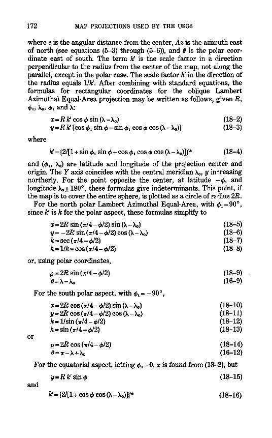
172 MAP PROJECTIONS USED BY THE USGS
where cis the angular distance from the center, Az is the azimuth east of north (see equations (5-3) through (5-6)), and fJ is the poJar coordinate east of south. The term lC is the scale factor in a direction perpendicular to the radius from the center of the map, not a long the parallel, except in the polar case. The scale factor: hf in the dirr~ction of the radius equals 1//C. After combining with standard equati0ns, the formulas for rectangular coordinates for the oblique Lambert Azimuthal Equal-Area projection may be written as follows, given R, cp., Ac,, cp, and X:
x=R lC cos cJ> sin (X-Ac,) y=R lC [cos cp1 sin cp- sin cp1 cos cJ> cos (X-Ac,)]
where
lC = {2/[1 +sin cp1 sin cJ> +cos cp1 cos cJ> cos (X- Ac,)]f12
(18-2) (18-3)
(18-4)
and (cp., Ac,) are latitude and longitude of the projection center and origin. The Y axis coincides with the central meridian Ac,, y in ~reasing northerly. For the point opposite the center, at latitude - cl>1 and longitude Ao± 180°, these formulas give indeterminants. This point, if the map is to cover the entire sphere, is plotted as a circle of radius 2R.
For the north polar Lambert Azimuthal Equal-Area, with cp1 = 90°, since lC is k for the polar aspect, these formulas simplify to
x = 2R sin ( r/4- cp/2) sin (X- Ac,) Y= -2R sin(r/4-cp/2)cos(X-Ac,) k= sec (r/4-q,/2) k= 1/k=cos(r/4-cp/2)
or, using polar coordinates,
p = 2R sin ( r/ 4- cp/2) 8=X-Ac,
For the south polar aspect, with cp, = - 90°,
X= 2R cos (r/4-cp/2) sin (X-Ac,)
or
y = 2R cos ( r/4- ¢/2) cos (X- Ac,) k= 1/sin(r/4-cp/2) k= sin ( r/4- cp/2)
p =2R cos (r/4-cp/2) 8=1r-X+Ac,
(18-5) (18-6) (18-7) (18-8)
(18-9) (16-9)
(18-10) (18-11) (18-12) (18-13)
(18-14) (16-12)
For the equatorial aspect, letting ¢ 1 = 0, x is found from (18-2), but
y=R lC sin cJ> (18-15) and
lC = {2/[1 +cos cp cos (X- Ac,)])lla (18-16)
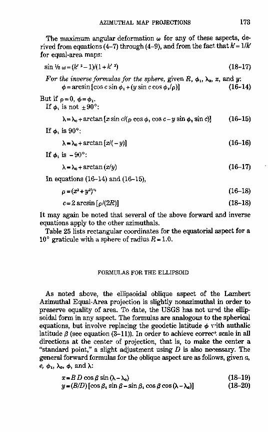
AZIMUTHAL MAP PROJECTIONS 173
The maximum angular deformation w for any of these aspects, derived from equations ( 4-7) through ( 4-9), and from the fact that h! = 1/~ for equal-area maps:
(18-17)
For the inverse formulas for the sphere, given R, cp., ~' x, and y: cf> =arcsin [cos c sin c/>1 + (y sin c cos ¢1/ p)] (16-14)
But if p=O, cf>=c/>1· If c/>1 is not ± 90°:
'h=~+arctan [x sin c/(p cos c/>1 cos c-y sin f/>1 sin c)]
If c/>1 is 90°:
'h=~+arctan [x/( -y)]
If c/>1 is -90°:
'h =~+arctan (xly)
In equations (16-14) and (16-15),
p =(Xl+yl)lh
c= 2 arcsin [p/(2R)]
(16-15)
(16-16)
(16-17)
(16-18)
(18-18)
It may again be noted that several of the above forward and inverse equations apply to the other azimuthals.
Table 25 lists rectangular coordinates for the equatorial aspect for a 10° graticule with a sphere of radius R = 1.0.
FORMULAS FOR THE ELLIPSOID
As noted above, the ellipsoidal oblique aspect of the Lambert Azimuthal Equal-Area projection is slightly nonazimuthal in order to preserve equality of area. To date, the USGS has not ur~d the ellipsoidal form in any aspect. The formulas are analogous to the spherical equations, but involve replacing the geodetic latitude q, Y·ith authalic latitude {3 (see equation (3-11)). In order to achieve correc~ scale in all directions at the center of projection, that is, to make the center a "standard point," a slight adjustment using Dis also ne~essary. The general forward formulas for the oblique aspect are as follows, given a, e, c/>1, ~' cf>, and 'h:
x=B D cos {3 sin ('h- Ao) Y= (BID) [cos {31 sin {3- sin {31 cos {3 cos (A-~)]
(18-19) (18-20)
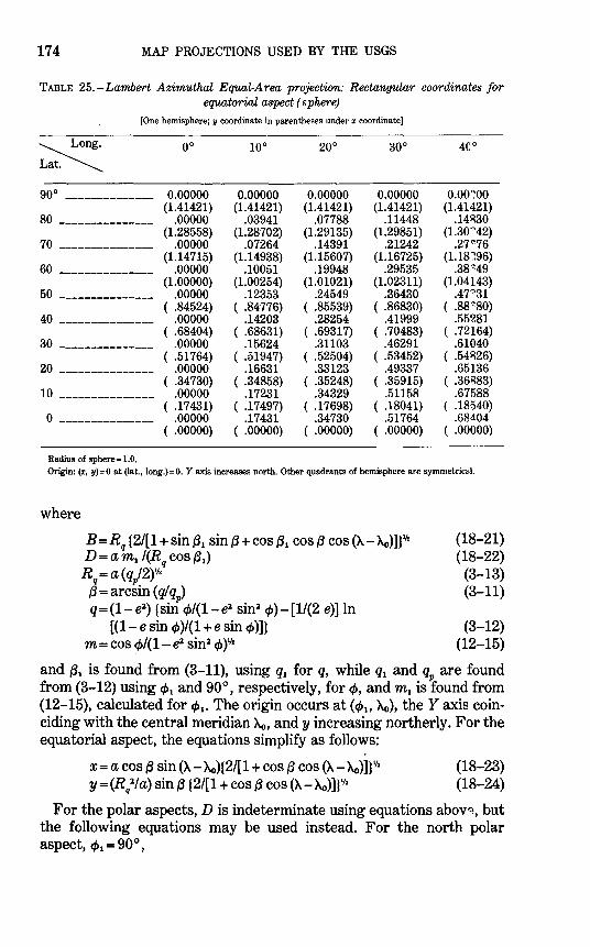
174 MAP PROJECTIONS USED BY THE USGS
TABLE 25.-Lamhert Azimuthal Equal-Area projection: Rectangular coordinates for equatorial aspect (sphere)
[One hemisphere; y coordinate in parentheses under x coordinate]
~ oo 100 20° 30° 4C 0
.
90° -------------- 0.00000 0.00000 0.00000 0.00000 o.oo;oo (1.41421) (1.41421) (1.41421) (1.41421) (1.41421)
80 --------------- .00000 .03941 .07788 .11448 .14~30 (1.28558) (1.28702) (1.29135) (1.29851) (1.30"42)
70 --------------- .00000 .07264 .14391 .21242 .27~76
(1.14715) (1.14938) (1.15607) (1.16725) (1.18;!96)
60 --------------- .00000 .10051 .19948 .29535 .38~49
(1.00000) (1.00254) (1.01021) (1.02311) (1.04143)
50 --------------- .00000 .12353 .24549 .36430 .47"31 ( .84524) ( .84776) ( .85539) ( .86830) ( .88~80)
40 --------------- .00000 .14203 .28254 .41999 .55?.81 ( .68404) ( .68631) ( .69317) ( .70483) ( .72164)
30 --------------- .00000 .15624 .31103 .46291 .61040 ( .51764) ( .51947) ( .52504) ( .53452) ( .54~26)
20 --------------- .00000 .16631 .33123 .49337 .65136 ( .34730) ( .34858) ( .35248) ( .35915) ( .36~83)
10 --------------- .00000 .17231 .34329 .51158 .67588 ( .17431) ( .17497) ( .17698) ( .18041) ( .18640)
0 --------------- .00000 .17431 .34730 .51764 .68404 ( .00000) ( .00000) ( .00000) ( .00000) ( .00000)
Radius of sphere= 1.0. Origin: (x, y)=O at (lat., long.)=O. Y axis increases north. Other quadrants of hemisphere are symmetrical.
where
B =Rq {2/[1 +sin {j1 sin {j +cos {j1 cos {j cos (A- Ac,)]}v2
D =a m1 I(Rq cos /j1)
R = a(q /2)112 q P,
{j = arcsin ( ql qP) q = (1- e2
) {sin (j>/(1- e1 sin2 4>)- [1/(2 e)] ln [(1- e sin 4>)/(1 + e sin 4>)]}
m= cos (j>/(1- & sin2 4>Y/2
(18-21) (18-22)
(3-13) (3-11)
(3-12) (12-15)
and /j1 is found from (3-11), using q1 for q, while q1 and q are found from (3-12) using (j> 1 and 90°, respectively, for (j>, and m1 is lfound from (12-15), calculated for (j> 1 • The origin occurs at (4>1, Ac,), theY axis coinciding with the central meridian Ac,, andy increasing northerly. For the equatorial aspect, the equations simplify as follows:
x =a cos {j sin (A- Ac,)[2/[1 +cos {j cos (A- Ac,)]f12
y=(R/Ia) sin {3 [2/[1 +cos {j cos (A- Ac,)Jr12
(18-23) (18-24)
For the polar aspects, D is indeterminate using equations abov~, but the following equations may be used instead. For the north polar aspect, {j> 1 = 90°,
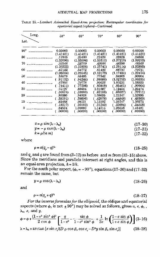
AZIMUTHAL MAP PROJECTIONS 175
TABLE 25.-Lambert Azimuthal Equal-Area projection: Rectangular coordinates for equatorial aspect (sphere)- Continued
~ 50° 60° 70° goo 90°
.
90° -------------- 0.00000 0.00000 0.00000 0.00000 0.00000 (1.41421) (1.41421) (1.41421) (1.41421) (1.41421)
80 --------------- .17843 .20400 .22420 .23828 .24558 (1.32096) (1.33594) (1.35313) (1.37219) (1.39273)
70 --------------- .33548 .38709 .43006 .46280 .48369 (1.20323) (1.22806) (1.25741) (1.29114) (1.32893)
60 --------------- .47122 .54772 .61403 .66797 .70711 (1.06544) (1.09545) (1.13179) (1.17481) (1.22474)
50 --------------- .58579 .68485 .77342 .84909 .90904 ( .91132) ( .94244) ( .98088) (1.02752) (1.08335)
40 --------------- .67933 .79778 .90620 1.00231 1.08335 ( .74411) ( .77298) ( .80919) ( .85401) ( .90904)
30 --------------- .75197 .88604 1.01087 1.12454 1.22474 ( .56674) ( .59069) ( .62108) ( .65927) ( .70711)
20 --------------- .80380 .94928 1.08635 1.21347 1.32893 ( .38191) ( .39896) ( .42078) ( .44848) ( .48369)
10 --------------- .83488 .98731 1.13192 1.26747 1.39273 ( .19217) ( .20102) ( .21240) ( .22694) ( .24558)
0 --------------- .84524 1.00000 1.14715 1.28558 1.41421 ( .00000) ( .00000) ( .00000) ( .00000) ( .00000)
x = p sin (A- Ao) (17-30) Y=- p cos (A- Ao) (17-31) k= pi( am) (17-32)
where
p = a(qp- q)¥2 (18-25)
and qP and q are found from (3-12) as before and m from (12-15) above. Since the meridians and parallels intersect at right angles, and this is an equal-area projection, h = 1/ k.
For the south polar aspect, (c/>1 =- 90°), equations (17-30) and (17-32) remain the same, but
y = p cos (A- Ao) (18-26)
and
(18-27) For the inverse formulas for the ellipsoid, the oblique and equatorial
aspects (where c/> 1 is not ± 90°) may be solved as follows, given a, e, cp1 ,
Ao, x, andy.
c/>=c/>+ (1-e2
sin2
cp)2 [~q- sin~ +_!_ ln (1-e s~n c/>)] (3_16)
2 cos cp 1- e2 1- e2 sm2 cp 2e 1 + e Sin cp
A= Ao +arctan [x sin cj(D p cos {3 1 cos ce- D 2y sin {3 1 since)] (18-28)
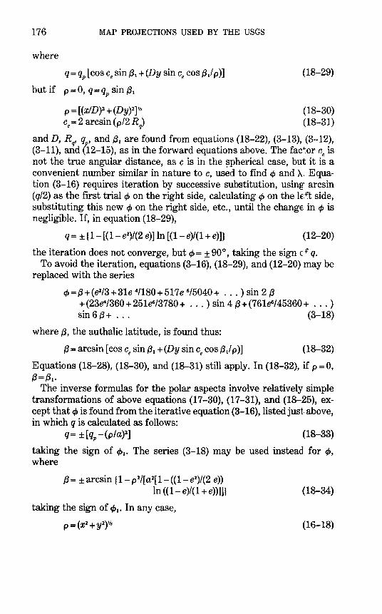
176 MAP PROJECTIONS USED BY THE USGS
where
q= qp [cos ce sin {31 + (Dy since cos {3 11 p)]
but if p = 0, q= qP sin {31
(18-29)
P = [(x/D)2 + (Dy)2f'2 ce= 2 arcsin (p/2 Rq)
(18-30) (18-31)
and D, Rq~ q , and {31 are found from equations (18-22), (3-13), (3-12), (3-11), and (12-15), as in the forward equations above. The fac1;or ce is not the true angular distance, as c is in the ~pherical case, but it is a convenient number similar in nature to c, used to find cp and A. Equation (3-16) requires iteration by successive substitution, using arcsin ( q/2) as the first trial cp on the right side, calculating cp on the l€ft side, substituting this new cp on the right side, etc., until the change. in cp is negligible. If, in equation (18-29),
q= ± {1- [(1- e2)/(2 e)] ln [{1- e)/(1 +e)]} (12-20)
the iteration does not converge, but cp = ± 90°, taking the sign c f q. To avoid the iteration, equations (3-16), (18-29), and (12-20) may be
replaced with the series
cp=f3+(e213+31e 4/180+517e 6/5040+ ... ) sin 2 {3 +(23~/360+251~/3780+ 0. 0) sin 4 {3+(761e6/45360+ 0. 0) sin 6 {3 + .. 0 (3-18)
where {3, the authalic latitude, is found thus:
{3= arcsin [cos ce sin {31 +(Dy since cos {3 1/p)] (18-32)
Equations (18-28), (18-30), and (18-31) still apply. In (18-32), if p = 0, {3={3.0
The inverse formulas for the polar aspects involve relatively simple transformations of above equations (17-30), (17-31), and (18-25), except that cp is found from the iterative equation (3-16), listed just above, in which q is calculated as follows:
q = ± [ qP- (pi a)2] (18-33)
taking the sign of cp1 o The series (3-18) may be used instead for cp, where
{3 = ±arcsin (1- p2/[ a 2[1- ((1- e2)/(2 e))
ln ((1- e)/(1 +e))]]}
taking the sign of cp1• In any case,
p=(X2+y2yh
(18-34)
(16-18)
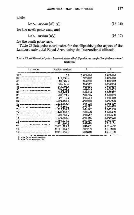
AZIMUTHAL MAP PROJECTIONS
while
A=Ao+arctan [xl( -y)]
for the north polar case, and
}.. = Ao +arctan (x/y)
for the south polar case.
177
(16-16)
(16-17)
Table 26 lists polar coordinates for the ellipsoidal polar as:'1ect of the Lambert Azimuthal Equal-Area, using the International elliosoid.
TABLE 26.-Ellipsoidal polar Lambert Azimuthal Equal-Area projection (International ellipsoid)
Latitude
90° --------------------89 ---------------------88 ____________________ _
8 7 ---------------------86 ---------------------85 ---------------------84 ---------------------83 ---------------------82 ---------------------81 ---------------------80 ____________________ _
79 ---------------------78 ---------------------77 ---------------------76 ---------------------7 5 ---------------------7 4 ---------------------73 ---------------------72 ---------------------71 ---------------------70 ---------------------
h = scale factor along meridian. k = scale factor along parallel.
Radius, meters
0.0 111,698.4 223,387.7 335,058.5 446,701.8 558,308.3 669,868.8 781,374.2 892,815.4
1,004,183.1 1,115,468.3 1,226,661.9 1,337,754.7 1,448,737.6 1,559,601.7 1,670,337.9 1,780,937.2 1,891,390.6 2,001,689.2 2,111,824.0 2,221,786.2
h
1.000000 .999962 .999848 .999657 .999391 .999048 .998630 .998135 .997564 .996918 .996195 .995397 .994522 .993573 .992547 .991446 .990270 .989018 .987691 .986289 .984812
k
1.000000 1.000038 1.000152 1.000343 1.000610 1.000953 1.001372 1.001869 1.002442 1.003092 1.003820 1.004625 1.005508 1.006469 1.007509 1.008628 1.009826 1.011104 1.012462 1.013902 1.015422

19. AZIMUTHAL EQUIDISTANT PROJECTION
SUMMARY
• Azimuthal. • Distances measured from the center are true. • Distances not measured along radii from the center are not correct. • The center of projection is the only point without distortion. • Directions from the center are true (except on some oblique and equatcrial ellipsoidal
forms). • Neither equal-area nor conformal. • All meridians on the polar aspect, the central meridian on other aspects, and the
Equator on the equatorial aspect are straight lines. • Parallels on the polar projection are circles spaced at true intervals (equidistant for
the sphere). • The outer meridian of a hemisphere on the equatorial aspect (for the sph::re) is a circle. • All other meridians and parallels are complex curves. • Not a perspective projection. • Point opposite the center is shown as a circle (for the sphere) surrounding the map. • Used in the polar aspect for world maps and maps of polar hemisphere.s. • Used in the oblique aspect for atlas maps of continents and world maps for aviation
and radio use. • Known for many centuries in the polar aspect.
HISTORY
While the Orthographic is probably the most familiar aziJnuthal projection, the Azimuthal Equidistant, especially in its polar form, has found its way into many atlases with the coming of the air age for maps of the Northern and Southern Hemispheres or for world maps. The simplicity of the polar aspect for the sphere, with equally spaced meridians and equidistant concentric circles for parallels of latitude, has made it easier to understand than most other projections. 'P1e primary feature, showing distances and directions correctly from 0'1e point on the Earth's surface, is also easily accepted. In addition, its linear scale distortion is moderate and falls between that of equal-area and conformal projections.
Like the Orthographic, Stereographic, and Gnomonic projections, the Azimuthal Equidistant was apparently used centuries before the 15th-century surge in scientific mapmaking. It is believed that Egyptians used the polar aspect for star charts, but the old€:st existing celestial map on the projection was prepared in 1426 by Cor~ad of Dyffenbach. It was also used in principle for small areas by mariners from earliest times in order to chart coasts, using distances anc directions obtained at sea.
179
180 MAP PROJECTIONS USED BY THE USGS
The first clear examples of the use of the Azimuthal Equidi~tant for polar maps of the Earth are those included by Gerhardus Mer~ator as insets on his 1569 world map, which introduced his famous cylindrical projection. As Northern and Southern Hemispheres, the projection appeared in a manuscript of about 1510 by the Swiss Henricus Loritus, usually called Glareanus (1488-1563), and by several others in the next few decades (Keuning, 1955, p. 4-5). Guillaume Postel is given credit in France for its origin, although he did not use it until 1581. Antonio Cagnoli even gave the projection his name as originator in 179':? (Deetz and Adams, 1934, p. 163; Steers, 1970, p. 234). Philippe Hatt developed ellipsoidal versions of the oblique aspect which are used by the French and the Greeks for coastal or topographic mapping.
Two projections with similar names are called the Tvro-Point Azimuthal and the Two-Point Equidistant projections. Both were developed about 1920 independently by Maurer (1919) of Germ~ny and Close (1921) of England. The first projection (rarely used) is geometrically a tilting of the Gnomonic projection to proV.de true azimuths from either of two chosen points instead of from j'lSt one. Like the Gnomonic, it shows all great circle arcs as straight lines and is limited to one hemisphere. The Two-Point Equidistant has received moderate use and interest, and shows true distances, but not true azimuths, from either of two chosen points to any other point on the map, which may be extended to show the entire world (Close, 1934).
The Chamberlin Trimetric projection is an approximate "thr~e-point equidistant" projection, constructed so that distances frmn three chosen points to any other point on the map are approximately correct. The latter distances cannot be exactly true, but the projection ic;; a compromise which the National Geographic Society uses as a stand~rd projection for maps of most continents. This projection was geomo.trically constructed by the Society, of which Wellman Chamberlin (1908-76) was chief cartographer for many years.
An ellipsoidal adaptation of the Two-Point Equidistant was made by Jay K. Donald of American Telephone and Telegraph Company in 1956 to develop a grid still used by the Bell Telephone syst~m for establishing the distance component of long distance rates. Still another approach is Bomford's modification of the Azimuthal Equidistant, in which the usual circles of constant scale factor perpendicular to the radius from the center are made ovals to give a better avera1e scale factor on a map with a rectangular border (Lewis and Campbe1l, 1951, p. 7, 12-15).
FEATURES
The Azimuthal Equidistant projection, like the Lambert Arjmuthal Equal-Area, is not a perspective projection, but in the spheric::-.l form,
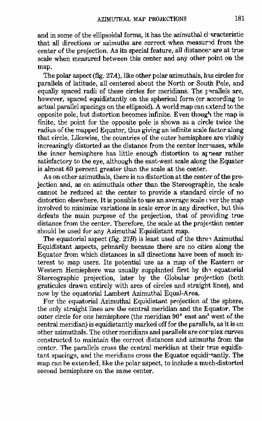
AZIMUTHAL MAP PROJECTIONS 181
and in some of the ellipsoidal forms, it has the azimuthal ch~racteristic that all directions or azimuths are correct when measur~d from the center of the projection. As its special feature, all distance~ are at true scale when measured between this center and any other point on the map.
The polar aspect (fig. 27A), like other polar azimuthals, has circles for parallels of latitude, all centered about the North or South Pole, and equally spaced radii of these circles for meridians. The IJ ~.rallels are, however, spaced equidistantly on the spherical form (or according to actual parallel spacings on the ellipsoid). A world map can extend to the opposite pole, but distortion becomes infinite. Even thoug1. the map is finite, the point for the opposite pole is shown as a circle twice the radius of the mapped Equator, thus giving an infinite scale factor along that circle. Likewise, the countries of the outer hemisphere are visibly increasingly distorted as the distance from the center incr~ases, while the inner hemisphere has little enough distortion to aJ: 1'1ear rather satisfactory to the eye, although the east-west scale along the Equator is almost 60 percent greater than the scale at the center.
As on other azimuthals, there is no distortion at the center of the projection and, as on azimuthals other than the Stereographic, the scale cannot be reduced at the center to provide a standard circle of no distortion elsewhere. It is possible to use an average scale C'ver the map involved to minimize variations in scale error in any direction, but this defeats the main purpose of the projection, that of providing true distance from the center. Therefore, the scale at the proje~tion center should be used for any Azimuthal Equidistant map.
The equatorial aspect (fig. 27B) is least used of the thre~ Azimuthal Equidistant aspects, primarily because there are no cities along the Equator from which distances in all directions have been of much interest to map users. Its potential use as a map of the Eastern or Western Hemisphere was usually supplanted first by th~ equatorial Stereographic projection, later by the Globular projE'etion (both graticules drawn entirely with arcs of circles and straight lines), and now by the equatorial Lambert Azimuthal Equal-Area.
For the equatorial Azimuthal Equidistant projection of the sphere, the only straight lines are the central meridian and the Equator. The outer circle for one hemisphere (the meridian 90° east ancl west of the central meridian) is equidistantly marked off for the paralle:ls, as it is on other azimuthals. The other meridians and parallels are corplex curves constructed to maintain the correct distances and azimuths from the center. The parallels cross the central meridian at their t:rue equidistant spacings, and the meridians cross the Equator equidi<:'t.antly. The map can be extended, like the polar aspect, to include a much-distorted second hemisphere on the same center.
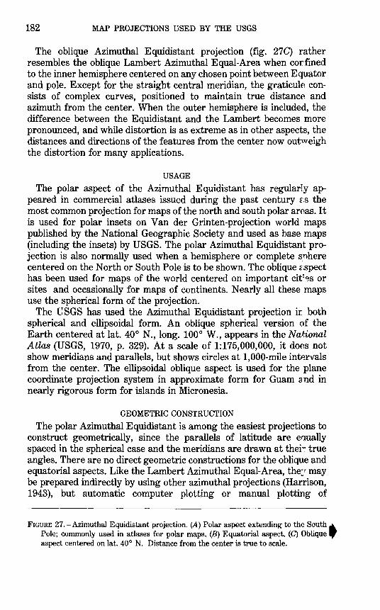
182 MAP PROJECTIONS USED BY THE USGS
The oblique Azimuthal Equidistant projection (fig. 27C) rather resembles the oblique Lambert Azimuthal Equal-Area when corfined to the inner hemisphere centered on any chosen point between Equator and pole. Except for the straight central meridian, the graticule consists of complex curves, positioned to maintain true distance and azimuth from the center. When the outer hemisphere is included, the difference between the Equidistant and the Lambert becomes more pronounced, and while distortion is as extreme as in other aspects, the distances and directions of the features from the center now outweigh the distortion for many applications.
USAGE
The polar aspect of the Azimuthal Equidistant has regularly appeared in commercial atlases issued during the past century f.s the most common projection for maps of the north and south polar areas. It is used for polar insets on Van der Grinten-projection world maps published by the National Geographic Society and used as base maps (including the insets) by USGS. The polar Azimuthal Equidistant projection is also normally used when a hemisphere or complete s:nhere centered on the North or South Pole is to be shown. The oblique f.spect has been used for maps of the world centered on important cit~o.s or sites and occasionally for maps of continents. Nearly all these maps use the spherical form of the projection.
The USGS has used the Azimuthal Equidistant projection in both spherical and ellipsoidal form. An oblique spherical version of the Earth centered at lat. 40° N., long. 100° W., appears in the National Atlas (USGS, 1970, p. 329). At a scale of 1:175,000,000, it does not show meridians and parallels, but shows circles at 1,000-mile intervals from the center. The ellipsoidal oblique aspect is used for the plane coordinate projection system in approximate form for Guam and in nearly rigorous form for islands in Micronesia.
GEOMETRIC CONSTRUCTION
The polar Azimuthal Equidistant is among the easiest projections to construct geometrically, since the parallels of latitude are equally spaced in the spherical case and the meridians are drawn at thei~ true angles. There are no direct geometric constructions for the oblique and equatorial aspects. Like the Lambert Azimuthal Equal-Area, the:r may be prepared indirectly by using other azimuthal projections (Harrison, 1943), but automatic computer plotting or manual plotting of
FIGURE 27.-Azimuthal Equidistant projection. (A) Polar aspect extending to the South._ Pole; commonly used in atlases for polar maps. (B) Equatorial aspect. (C) Oblique .,aspect centered on lat. 40° N. Distance from the center is true to scale.
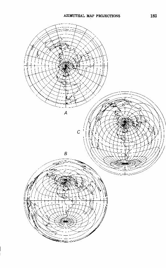
AZIMUTHAL MAP PROJECTIONS 183
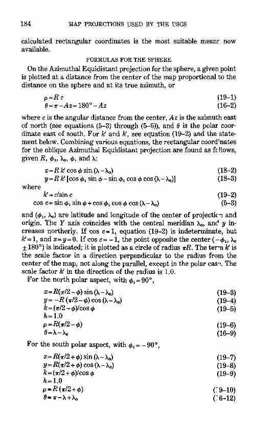
184 MAP PROJECTIONS USED BY THE USGS
calculated rectangular coordinates is the most suitable meanr now available.
FORMULAS FOR THE SPHERE
On the Azimuthal Equidistant projection for the sphere, a given point is plotted at a distance from the center of the map proportional to the distance on the sphere and at its true azimuth, or
p=Rc 8= 1r-Az= 180° -Az
(19-1) (16-2)
where cis the angular distance from the center, Az is the azimuth east of north (see equations (5-3) through (5-6}), and 8 is the polar coordinate east of south. For 1C and h:, see equation (19-2) and the statement below. Combining various equations, the rectangular coord:nates for the oblique Azimuthal Equidistant projection are found as fc llows, given R, <Ph Ao, </>, and A:
x = R 1C cos <1> sin (A- Ao) y = R 1C [cos </>1 sin <1>- sin </>1 cos <1> cos (A- Ao)]
where
(18-2) (18-3)
1C = c/sin c (19-2) cos c = sin </>1 sin <1> +cos </>1 cos q, cos (A- Ao) (5-3)
and ( </>1, Ao) are latitude and longitude of the center of projectk'1 and origin. The Y axis coincides with the central meridian Ao, anc1 y increases northerly. If cos C= 1, equation (19-2) is indeterminate, but IC= 1, and x=y=O. If cos C= -1, the point opposite the center (-<Ph he> ± 180°) is indicated; it is plotted as a circle of radius 1rR. The ter'tllC is the scale factor in a direction perpendicular to the radius from the center of the map, not along the parallel, except in the polar cas~. The scale factor h: in the direction of the radius is 1.0.
For the north polar aspect, with <J>1 = 90°,
x=R(7r/2-</>) sin (A- Ao) y = - R ( 1r/2- </>) cos (A- Ao) k= (1rl2- q,)/cos q, h=l.O p =R(1r/2- </>) 8=A-Ao
For the south polar aspect, with <J> 1 = - 90°,
x=R(7ri2+<P) sin (A- Ao) y = R( 1r/2 + <1>) cos (A- Ao) k= (1r/2 + q,)/cos q, h=l.O p =R (7rl2+</>) 8= 7r-A+Ao
(19-3) (19-4) (19-5)
(19-6) (16-9)
(19-7) (19-8) (19-9)
(:'.9-10) (l6-12)
AZIMUTHAL MAP PROJECTIONS 185
For the equatorial aspect, with ¢1 = 0, xis found from (18-2) and It from (19-2), but
y=R lC sin¢ (19-11)
and
cos C= cos¢ cos (A- Ao) (19-12)
The maximum angular deformation w for any of these aspects, using equations (4-7) through (4-9), since h!= 1.0:
sin 1hw =(It -1)/(/t + 1) = (c- sin c)/(c+ sin c)
(19-13) (19-14)
For the inverse formulas for the sphere, given R, t/J1 , Xo, x, 8 nd y:
t/J=arcsin [cos c sin ¢1 +(y sin c cos ¢ 1/p)] (16-14)
But if p=O, ¢=¢~. If ¢ 1 is not ± 90°:
A= Xo +arctan [x sin c!( p cos ¢ 1 cos c- y sin ¢ 1 sin c)]
If ¢ 1 is 90°:
A= Xo +arctan [x/(- y)]
If ¢ 1 is -90°:
A= Xo +arctan (x/y)
In equations (16-14) and (16-15),
P =(x2+Y2rlz C=piR
(16-15)
(16-16)
(16-17)
(16-18) (19-15)
Except for (19-15), the above inverse formulas are the same as those for the other azimuthals, and (19-2) is the only change from previous azimuthals among the general (oblique) formulas (18-2) through (5-3) for the forward calculations as listed above.
Table 27 shows rectangular coordinates for the equatorial aspect for a 10° graticule with a sphere of radius R = 1.0.
FORMULAS FOR THE ELLIPSOID
The formulas for the polar aspect of the ellipsoidal Azimuthal Equidistant projection are relatively simple and are theoretically accurate for a map of the entire world. However, such a use is unnecessary because the errors of the sphere versus the ellipsoid become insignificant when compared to the basic errors of projection. The

186 MAP PROJECTIONS USED BY THE USGS
TABLE 27. -Azimuthal Equidistant projection: Rectangular coordinates for equatorial aspect (sphere)
[One hemisphere; R= 1. y coordinates in parentheses under x coordinates]
~ oo 100 20° 30° 40°
.
90° -------------- 0.00000 0.00000 0.00000 0.00000 c.ooooo
80 ---------------(1.57080) (1.57080) (1.57080) (1.57080) (1.57080)
.00000 .04281 .08469 .12469 .16188
70 ------------(1.39626) (1.39829) (1.40434) (1.41435) (1.42823)
.00000 .07741 .15362 .22740 .29744
60 ----~~--------(1.22173) (1.22481) (1.23407) (1.24956) (1.27137)
.00000 .10534 .20955 .31145 .40976
50 ---------------(1.04720) (1.05068) (1.06119) (1.07891) (1.10415)
.00000 .12765 .25441 .37931 .50127
40 ---------------( .87266) ( .87609) ( .88647) ( .90408) ( .92938)
.00000 .14511 .28959 .43276 .57386
30 ---------------( .69813) ( .70119) ( .71046) ( .72626) ( .74912)
.00000 .15822 .31607 .47314 .62896
20 ---------------( .52360) ( .52606) ( .53355) ( .54634) ( .56493)
.00000 .16736 .33454 .50137 .66762
10 ---------------( .34907) ( .35079) ( .35601) ( .36497) ( .37803)
.00000 .17275 .34546 .51807 .69054
0 ---------------( .17453) ( .17541) ( .17810) ( .18270) ( .18943)
.00000 .17453 .34907 .52360 .69813 ( .00000) ( .00000) ( .00000) ( .00000) ( .00000)
TABLE 27.-Azimuthal Equidistant projection: Rectangular coordinates for e~-;uatorial aspect (sphere)- Continued
~ 50° 60° 70° 80° 90° .
90° -------------- 0.00000 0.00000 0.00000 0.00000 0.00000 (1.57080) (1.57080) (1.57080) (1.57080) (1.57080)
80 --------------- .19529 .22399 .24706 .26358 .27277 (1.44581) (1.46686) (1.49104) (1.51792) (1.54693)
70 --------------- .36234 .42056 .47039 .50997 .53724 (1.29957) (1.33423) (1.37533) (1.42273) (1.47607)
60 --------------- .50301 .58948 .66711 .73343 .78540 (1.13733) (1.17896) (1.22963) (1.28993) (1.36035)
50 --------------- .61904 .73106 .83535 .92935 1.00969 ( .96306) (1.00602) (1.05942) (1.12464) (1.20330)
40 --------------- .71195 .84583 .97392 1.09409 1.20330 ( .77984) ( .81953) ( .86967) ( .93221) (1.00969)
30 --------------- .78296 .93436 1.08215 1.22487 1.36035 ( .59010) ( .62291) ( .66488) ( .71809) ( .78540)
20 --------------- .83301 .99719 1.15965 1.31964 1.47607 ( .39579) ( .41910) ( .44916) ( .48772) ( .53724)
10 --------------- .86278 1.03472 1.20620 1.37704 1.54693 ( .19859) ( .21067) ( .22634) ( .24656) ( .27277)
0 --------------- .87266 1.04720 1.22173 1.39626 1.57080 ( .00000) ( .00000) ( .00000) ( .00000) ( .00000)
Radius of sphere -1.0. Origin: (x, y)•O at (lat., long.)•O. Y axis increases north. Other quadrants of hemisphere are symmetlical.
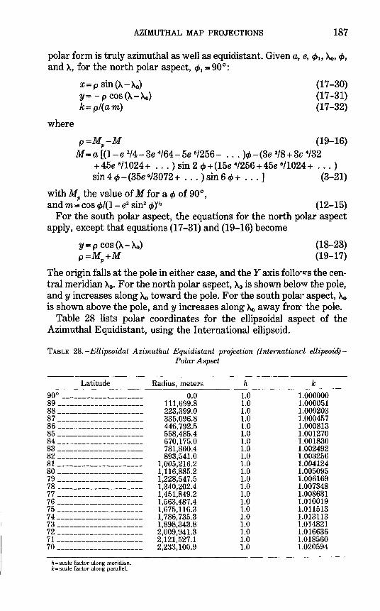
AZIMUTHAL MAP PROJECTIONS 187
polar form is truly azimuthal as well as equidistant. Given a, e, q,., he,, q,, and)., for the north polar aspect, c/> 1 =90°:
where
x = p sin (). - Ac,) y = - p cos ().-he,) k= p/(am)
(17-30) (17-31) (17-32)
p=Mp-M (19-16) M =a [(1- e 2/4- 3e 4/64- 5e 6/256- ... )cf>- (3e 2/8 + 3e 4/32
+ 45e 6/1024 + ... ) sin 2 q, + (15e 4/256 + 45e 6/1024 + ... ) sin 4 q,- (35e 6/3072 + ... ) sin 6 q, + ... ] (3-21)
with MP the value of M for a q, of 90°, and m= cos q,/(1- e2 sin2 q,)lf2 (12-15)
For the south polar aspect, the equations for the north polar aspect apply, except that equations (17-31) and (19-16) become
Y= p cos().- he,) p=Mp+M
(18-23) (19-17)
The origin falls at the pole in either case, and the Y axis follows the central meridian ~. For the north polar aspect, ~ is shown below the pole, and y increases along he, toward the pole. For the south pola1· aspect, he, is shown above the pole, and y increases along he, away frorr the pole.
Table 28 lists polar coordinates for the ellipsoidal aspect of the Azimuthal Equidistant, using the International ellipsoid.
TABLE 28. -Ellipsoidal Azimuthal Equidistant projection (lnternationcl ellipsoid)Polar Aspect
Latitude
90° --------------------89 ---------------------88 ---------------------87 ---------------------86 ____________________ _
85 ---------------------84 ---------------------83 ---------------------82 ---------------------81 ____________________ _
80 ---------------------79 ---------------------78 ---------------------77 ---------------------76 ---------------------75 ---------------------7 4 ---------------------73 ---------------------72 ---------------------71 ____________________ _
70 ---------------------
h = scale factor along meridian. k = scale factor along parallel.
Radius, meters
0.0 111,699.8 223,399.0 335,096.8 446,792.5 558,485.4 670,175.0 781,860.4 893,541.0
1,005,216.2 1,116,885.2 1,228,547.5 1,340,202.4 1,451,849.2 1,563,487.4 1,675,116.3 1,786,735.3 1,898,343.8 2,009,941.3 2,121,527.1 2,233,100.9
h
1.0 1.0 1.0 1.0 1.0 1.0 1.0 1.0 1.0 1.0 1.0 1.0 1.0 1.0 1.0 1.0 1.0 1.0 1.0 1.0 1.0
k
1.000000 1.000051 1.000203 1.000457 1.000813 1.001270 1.001830 1.002492 1.003256 1.004124 1.005095 1.006169 1.007348 1.008631 1.010019 1.011513 1.013113 1.014821 1.016636 1.018560 1.020594
188 MAP PROJECTIONS USED BY THE USGS
For the oblique and equatorial aspects of the ellipsoidal Azimuthal Equidistant, both nearly rigorous and approximate sets of formulas have been derived. For mapping of Guam, the National Geodetic Survey and the USGS use an approximation to the ellipsoidal oblique Azimuthal Equidistant called the "Guam projection." It is described by Claire (1968, p. 52-53) as follows (changing his symbols to match those in this publication):
"The plane coordinates of the geodetic stations on Guam were obtained by first computing the geodetic distances [c] and azimuths [Az] of all points from the origin by inverse computations. The coordinates were then computed by the equations: [x=c sin Az and y=c cos Az]. This really gives a true azimuthal equidistant projection. The equations given here are simpler, however, than those for a geodetic inverse computatio"l, and the resulting coordinates computed using them will not be significantly different f-om those computed rigidly by inverse computation. This is the reason it is called an ap:->roximate azimuthal equidistant projection."
The formulas for the Guam projection are equivalent to the following:
x=a(A-Ao) cos cp/(l-e2 sin2cJ>r12
y=M -M1 +X2 tan cp (1- e2 sin2 cp)'12/(2a) (19-18) (19-19)
where M and M 1 are found from equation (3-21) for cp and cp1 • Actually, the original formulas are given in terms of seconds of re~tifying latitude and geodetic latitude and longitude, but they may be written as above. The x coordinate is thus taken as the distance along the parallel, and y is the distance along the central meridian Ao with adjustment for curvature of the parallel. The origin occurs at (cp., Ao), theY axis coincides with the central meridian, andy increases northerly.
For Guam, c/> 1 = 13°28'20.87887" N. lat. and Ao= 144°44'55.50254" E. long., with 50,000 m added to both x and y to eliminate n~gative numbers. The Clarke 1866 ellipsoid is used.
A more complicated and more accurate approach to the oblique ellipsoidal Azimuthal Equidistant projection is used for plane coordinates of various individual islands of Micronesia. In this form, the true distance and azimuth of any point on the island or in nearby waters are measured from the origin chosen for the island and along the normal section or plane containing the perpendicular to the surface of the ellipsoid at the origin. This is not exactly the same as the shortest or geodesic distance between the points, but the difference is ne~ligible (Bomford, 1971, p. 125). This distance and azimuth are plotted on the map. The projection is, therefore, equidistant and azimuthal with respect to the center and appears to satisfy all the requirementr~ for an ellipsoidal Azimuthal Equidistant projection, although it is descr;bed as a "modified" form. The origin is assigned large-enough values of x andy to prevent negative readings.
AZIMUTHAL MAP PROJECTIONS 189
The formulas for calculation of this distance and azimuth have been published in various forms, depending on the maximum distance involved. The projection system for Micronesia makes use of "Clarke's best formula" and Robbins's inverse of this. These are considered suitable for lines up to 800 km in length. The formulas below, rearranged slightly from Robbins's formulas as given in Bomford (1971, p. 136-137), are extended to produce rectangular coordinates. No iteration is required. They are listed in the order of use, given a central point at lat. ~11 long. Ao, coordinates X0 and Yo of the central point, the Y axis along the central meridian Ao, y increasing northerl;T, ellipsoidal parameters a and e, and ~ and A.
To find x andy:
N. = a/(1- e2 sin2 ~S12
N = a/(1- e2 sin2 ~ )'12
1/; =arctan [(1- e2)tan ~ + e2 N 1 sin ~.I(N cos~)] Az= arctan {sin (A- Ao)/[cos ~~tan 1/;- sin~~ cos (A- Ao)]}
(4-20a) (4-20)
(19-20) (19-21)
The ATAN2 Fortran function should be used with equation (19-21), but it is not applicable to (19-20).
If sin Az=O,
s= ± arcsin(cos¢1 sin,P-sin~1 cos,P)
taking the sign of cos Az. If sin Az=1=0,
s= arcsin [sin (A- Ao) cos ,PisinAz]
In either case,
G = e sin ~1/(1- e2}'
12
H = e cos ~1 cos Az/(1- e2)'12
c = N 1 s{ 1- s2H 2(1- H 2)/6 + ( s3/8)GH(1- 2H2)
+(s4/120)[H2{4-7H2)- 3G2{1-7H2)]
- (s5/48)GH} X= c sinAz+X0
Y=CCOSAZ+Yo
(19-22)
(19-22a)
(19-23) (19-24)
(19-25) (19-26) (19-27)
where c is the geodetic distance, and Az is azimuth east of north. Table 29 shows the parameters for the various islands 1napped with
this projection. Inverse formulas for the polar ellipsoidal aspect, given tr.., e, ~11 Ao, x,
andy:
~=p.+(3e1/2-27 eU32) sin 2p.+(21 ef/16-55 et/32) r1n 4p. + (151 e:f96) sin 6p. + . . . (3-26)
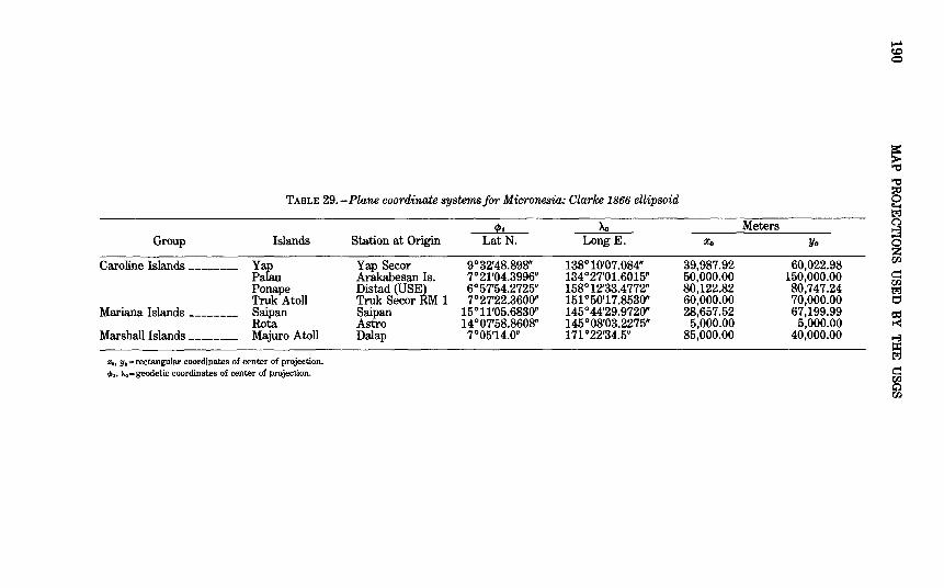
TABLE 29.-Plane coordinate systems for Micronesia: Clarke 1866 ellipsoid
9!.1 Xo Group Islands Station at Origin LatN. Long E.
Caroline Islands-------- y:fa Yap Secor 9° 32' 48.898" 138° 10'07.084" P au Arakabesan Is. 7°21'04.3996" 134 °27'01.6015" Po nape Distad (USE) 6°57'54.2725" 158°12'33.4772" Truk Atoll Truk Secor RM 1 7°27'22.3600" 151 °50'17.8530"
Mariana Islands -------- Saipan Saipan 15°11'05.6830" 145 ° 44'29 .9720" Rota Astro 14 °07'58.8608" 145°08'03.2275"
Marshall Islands -------- Majuro Atoll Dalap 7°05'14.0" 171 °22'34.5"
x,, Yo= rectangular coordinates of ct>nter of projection. q,,, llo =geodetic coordinates of center of projection.
Meters Xo Yo
39,987.92 60,022.98 50,000.00 150,000.00 80,122.82 80,747.24 60,000.00 70,000.00 28,657.52 67,199.99
5,000.00 5,000.00 85,000.00 40,000.00
"'"""' cc 0
~ ., ~ t;a C"l
~ rn c::: rn t.:t:j I:'
~ t-3 g; c::: rn ~
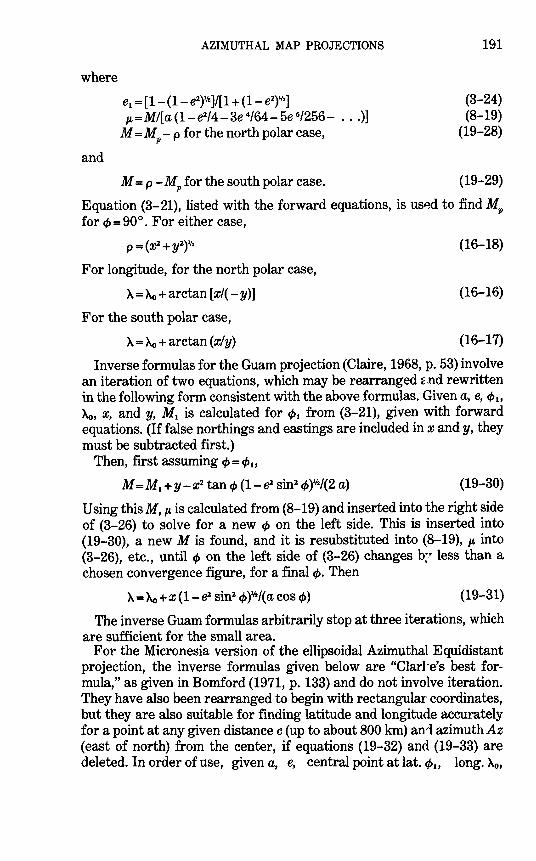
where
and
AZIMUTHAL MAP PROJECTIONS
e.= [1- (1- e1Y12 ]/[1 + (1- e2r'2 1 p. =MI[ a (1- e214- 3e 4/64- 5e 6/256- ... )]
M = MP- p for the north polar case,
M = p-MP for the south polar case.
191
(3-24) (8-19)
(19-28)
(19-29)
Equation (3- 21), listed with the forward equations, is usAd to find MP for ¢=90°. For either case,
p = (x2 + yl)lh (16-18)
For longitude, for the north polar case,
A=Ao+arctan [x/( -y)]
For the south polar case,
}.. = Ao +arctan (x/y)
(16-16)
(16-17)
Inverse formulas for the Guam projection (Claire, 1968, p. 53) involve an iteration of two equations, which may be rearranged ~nd rewritten in the following form consistent with the above formulas. Given a, e, c/> 1,
Ao, x, and y, M 1 is calculated for c/> 1 from (3-21), given with forward equations. (If false northings and eastings are included in x and y, they must be subtracted first.)
Then, first assuming cJ> = cJ>.,
(19-30)
Using this M, p. is calculated from (8-19) and inserted into the right side of (3-26) to solve for a new cJ> on the left side. This is inserted into (19-30), a new M is found, and it is resubstituted into (8-19), p. into (3-26), etc., until cf> on the left side of (3-26) changes b? less than a chosen convergence figure, for a final cJ>. Then
A=Ao+X (1-& sin2 cf>)lh/(a cos cJ>) (19-31)
The inverse Guam formulas arbitrarily stop at three iterations, which are sufficient for the small area.
For the Micronesia version of the ellipsoidal Azimuthal Equidistant projection, the inverse formulas given below are "Clarl·e's best formula," as given in Bomford (1971, p. 133) and do not involve iteration. They have also been rearranged to begin with rectangular coordinates, but they are also suitable for finding latitude and longitude accurately for a point at any given distance c (up to about 800 km) ani azimuthAz (east of north) from the center, if equations (19-32) and (19-33) are deleted. In order of use, given a, e, central point at lat. ¢., long. Ao,
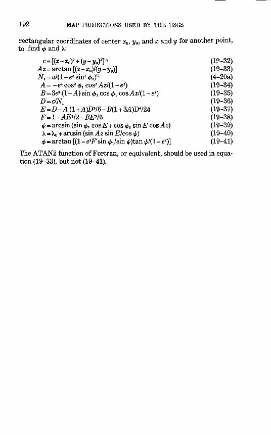
192 MAP PROJECTIONS USED BY THE USGS
rectangular coordinates of center x0 , y0 , and x and y for another point, to find <P and A:
c = [(x- Xo)2 + (y- Yo)l)V2 Az =arctan [(x- Xo)l(y- Yo)] N1 = a/(1- e1 sin1 <PStz A = - e1 cos1 <j} 1 cos1 Az/(1- e1)
B = 3e1 (1-A) sin <P 1 cos <P1 cosAz/(1- e1)
D=c!Nl E=D-A (l+A)D3/6-B(1+3A)D4/24 F= 1-AE1/2-BE3/6 ~=arcsin (sin <Pt cos E +cos <j} 1 sinE cos Az) A= Ao +arcsin (sin Az sinE/cos~) <P =arctan [(1- e1F sin <j}1/sin ~)tan ~/(1- e1
)]
(1~-32)
(19-33) (4-20a) (19-34) (19-35) (19-36) (19-37) (19-38) (19-39) (19-40) (19-41)
The ATAN2 function of Fortran, or equivalent, should be used in equation (19-33), but not (19-41).
SPACE MAP PROJECTIONS
One of the most recent developments in map projectiors has been that involving a time factor, relating a mapping satellite revolving in an orbit about a rotating Earth. With the advent of automated continuous mapping in the near future, the static projections previously available are not sufficient to provide the accuracy merited by the imagery, without frequent readjustment of projection parameters and discontinuity at each adjustment. Projections appropriate for such satellite mapping are much more complicated mathematically, but, once derived, can be handled by computer.
Several such space map projections have been conceived, and all but one have been mathematically developed. The Space Oblique Mercator projection, suitable for mapping imagery from Landzat and other vertically scanning satellites, is described below. The Space 01lique Conformal Conic is a still more complex projection, currently only in conception, but for which mathematical development will he required when satellite side-looking imagery has been developed to an extent sufficient to encourage its use. Satellite-tracking projections are simpler, but are less important and are not discussed her~ (Snyder, 1981a).
20. SPACE OBLIQUE MERCATOR PROJECTION
SUMMARY • Modified cylindrical projection with map surface defined by satellite orbit. • Designed especially for continuous mapping of satellite imagery. • Basically conformal, especially in region of satellite scanning. • Groundtrack of satellite, a curved line on the globe, is shown as a curv~d line on the
map and is continuously true to scale as orbiting continues. • All meridians and parallels are curved lines, except meridian at each polar approach. • Recommended only for a relatively narrow band along the groundtrack. • Developed 1973-79 by Colvocoresses, Snyder, and Junkins.
HISTORY
The launching of an Earth-sensing satellite by the National Aeronautics and Space Administration in 1972 led to a new era of mapping on a continuous basis from space. This satellite, first called ERTS-1 and renamed Landsat-1 in 1975, was followed by two others, all of which circled the Earth in a nearly circular orbit incrned about 99° to the Equator and scanning a swath about 185 km (oficially 100 nautical miles) wide from an altitude of about 919 km. A fo~1rth Landsat has somewhat different orbital parameters.
193
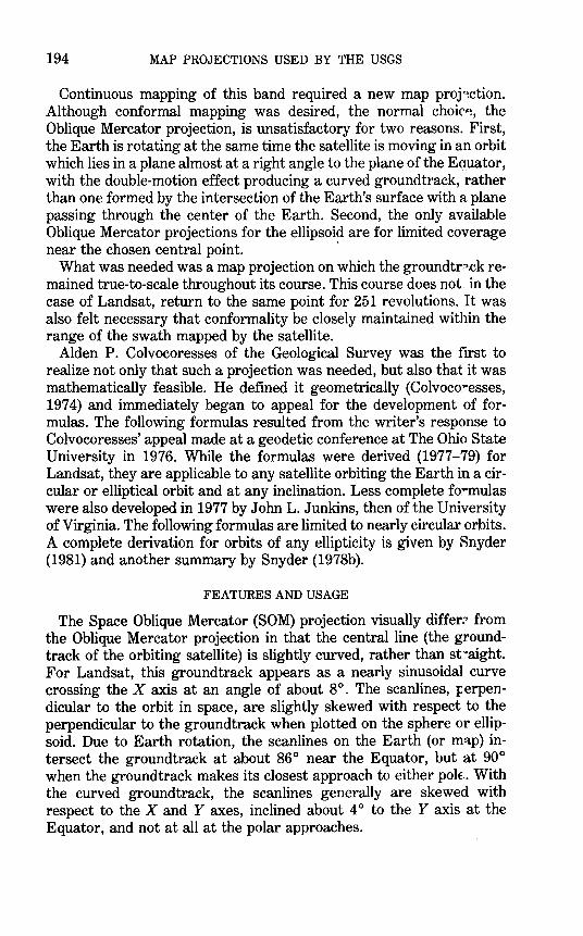
194 MAP PROJECTIONS USED BY THE USGS
Continuous mapping of this band required a new map proj~ction. Although conformal mapping was desired, the normal choir~, the Oblique Mercator projection, is unsatisfactory for two reasons. First, the Earth is rotating at the same time the satellite is moving in an orbit which lies in a plane almost at a right angle to the plane of the Eouator, with the double-motion effect producing a curved groundtrack, rather than one formed by the intersection of the Earth's surface with a plane passing through the center of the Earth. Second, the only available Oblique Mercator projections for the ellipsoid are for limited coverage near the chosen central point. ·
What was needed was a map projection on which the groundtr~.ck remained true-to-scale throughout its course. This course does not, in the case of Landsat, return to the same point for 251 revolutions. It was also felt necessary that conformality be closely maintained within the range of the swath mapped by the satellite.
Alden P. Colvocoresses of the Geological Survey was the first to realize not only that such a projection was needed, but also that it was mathematically feasible. He defined it geometrically (Colvoco:--esses, 1974) and immediately began to appeal for the development of formulas. The following formulas resulted from the writer's response to Colvocoresses' appeal made at a geodetic conference at The Ohio State University in 1976. While the formulas were derived (1977-79) for Landsat, they are applicable to any satellite orbiting the Earth in a circular or elliptical orbit and at any inclination. Less complete fo:--mulas were also developed in 1977 by John L. Junkins, then of the University of Virginia. The following formulas are limited to nearly circular orbits. A complete derivation for orbits of any ellipticity is given by Snyder (1981) and another summary by Snyder (1978b).
FEATURES AND USAGE
The Space Oblique Mercator (SOM) projection visually differ;;- from the Oblique Mercator projection in that the central line (the groundtrack of the orbiting satellite) is slightly curved, rather than st:-:-aight. For Landsat, this groundtrack appears as a nearly sinusoidal curve crossing the X axis at an angle of about 8°. The scanlines, perpendicular to the orbit in space, are slightly skewed with respect to the perpendicular to the groundtrack when plotted on the sphere or ellipsoid. Due to Earth rotation, the scanlines on the Earth (or m~p) intersect the groundtrack at about 86° near the Equator, but at 90° when the groundtrack makes its closest approach to either pole:. With the curved groundtrack, the scanlines generally are skewed with respect to the X and Y axes, inclined about 4 o to the Y axis at the Equator, and not at all at the polar approaches.
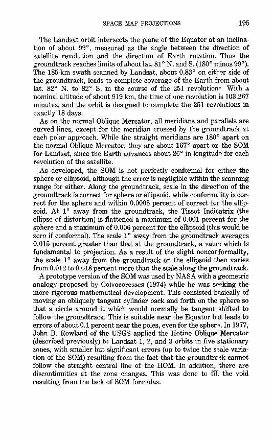
SPACE MAP PROJECTIONS 195
The Landsat orbit intersects the plane of the Equator at an inclination of about 99°, measured as the angle between the direction of satellite revolution and the direction of Earth rotation. Thus the groundtrack reaches limits of about lat. 81 oN. and S. (180° minus 99°). The 185-km swath scanned by Landsat, about 0.83° on eitl,~r side of the groundtrack, leads to complete coverage of the Earth from about lat. 82° N. to 82° S. in the course of the 251 revolution<:', With a nominal altitude of about 919 km, the time of one revolution is 103.267 minutes, and the orbit is designed to complete the 251 revolutions in exactly 18 days.
As on the normal Oblique Mercator, all meridians and parallels are curved lines, except for the meridian crossed by the groundtrack at each polar approach. While the straight meridians are 180° apart on the normal Oblique Mercator, they are about 167° apart Oil the SOM for Landsat, since the Earth advances about 26° in longitud~ for each revolution of the satellite.
As developed, the SOM is not perfectly conformal for either the sphere or ellipsoid, although the error is negligible within the scanning range for either. Along the ground track, scale in the direction of the ground track is correct for sphere or ellipsoid, while conformzlity is correct for the sphere and within 0.0005 percent of correct for the ellipsoid. At 1 o away from the groundtrack, the Tissot Indicatrix (the ellipse of distortion) is flattened a maximum of 0.001 percent for the sphere and a maximum of 0.006 percent for the ellipsoid (this would be zero if conformal). The scale 1 o away from the groundtrack averages 0.015 percent greater than that at the groundtrack, a valu~ which is fundamental to projection. As a result of the slight nonconformality, the scale 1 o away from the groundtrack on the ellipsoid then varies from 0.012 to 0.018 percent more than the scale along the groundtrack.
A prototype version of the SOM was used by NASA with a geometric analogy proposed by Colvocoresses (1974) while he was SE'~king the more rigorous mathematical development. This consisted b1tsically of moving an obliquely tangent cylinder back and forth on the sphere so that a circle around it which would normally be tangent shifted to follow the groundtrack. This is suitable near the Equator but leads to errors of about 0.1 percent near the poles, even for the spher~~. In 1977, John B. Rowland of the USGS applied the Hotine Oblique Mercator (described previously) to Landsat 1, 2, and 3 orbits in five stationary zones, with smaller but significant errors (up to twice the S~'~ale variation of the SOM) resulting from the fact that the groundtrr~k cannot follow the straight central line of the HOM. In addition, there are discontinuities at the zone changes. This was done to fill the void resulting from the lack of SOM formulas.

y
--- SCAN LINES (EXTENDED 30°!
-- GROUNDTRACK
iY
FIGURE 28.- Two orbits of the Space Oblique Mercator projection, shown for Landsat. Designed for a narrow band along groundtrack, which remains true to scale. Note the change in longitude at a given latitude along the groundtrack, with successive orbits.
,__. ~ 0')
~ "'0 "'0
~ ~ l%j 0 1-3
~ 00
e 00 l%j
t:1 a; t-< 1-3 l:I1 l%j
e 00 c;':l 00
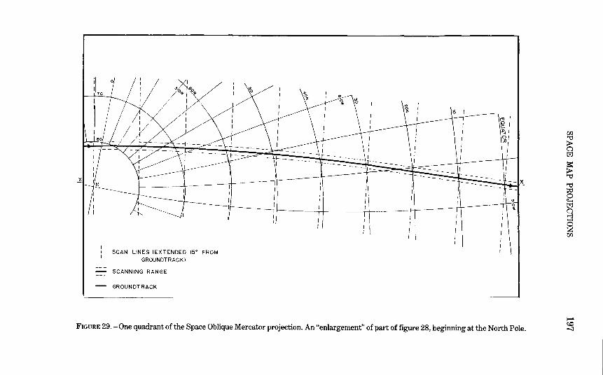
SCAN LINES !EXTENDED 15" FROM
GROUNDTRACKl
SCANNING RANGE
GROUNDTRACK
FIGURE 29.- One quadrant of the Space Oblique Mercator projection. An "enlargement" of part of figure 28, beginning at the North Pole.
en ""d > 0 tz:j
a:: > ""d
""d
~ t;j 0 1-3
~ en
1-l ~ -.:)
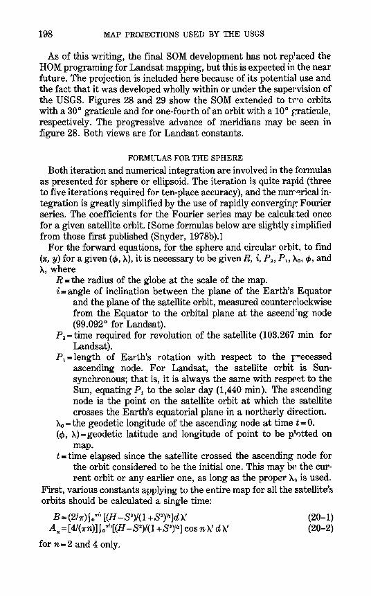
198 MAP PROJECTIONS USED BY THE USGS
As of this writing, the final SOM development has not rep]aced the HOM programing for Landsat mapping, but this is expected in the near future. The projection is included here because of its potential use and the fact that it was developed wholly within or under the supervision of the USGS. Figures 28 and 29 show the SOM extended to tFo orbits with a 30° graticule and for one-fourth of an orbit with a 10° graticule, respectively. The progressive advance of meridians may be seen in figure 28. Both views are for Landsat constants.
FORMULAS FOR THE SPHERE
Both iteration and numerical integration are involved in the formulas as presented for sphere or ellipsoid. The iteration is quite rapid (three to five iterations required for ten-place accuracy), and the nurr~rical integration is greatly simplified by the use of rapidly converging Fourier series. The coefficients for the Fourier series may be calculz.ted once for a given satellite orbit. [Some formulas below are slightly simplified from those first published (Snyder, 1978b).J
For the forward equations, for the sphere and circular orbit, to find (x, y) for a given(¢, A), it is necessary to be given R, i, P1 , Pu Ac,, ¢,and A, where
R =the radius of the globe at the scale of the map. i =angle of inclination between the plane of the Earth's Equator
and the plane of the satellite orbit, measured counterclockwise from the Equator to the orbital plane at the ascend~ng node (99.092° for Landsat).
P1 =time required for revolution of the satellite (103.267 min for Landsat).
P1 =length of Earth's rotation with respect to the r"'"ecessed ascending node. For Landsat, the satellite orbit is Sunsynchronous; that is, it is always the same with respE'~t to the Sun, equating P 1 to the solar day (1,440 min). The ascending node is the point on the satellite orbit at which the satellite crosses the Earth's equatorial plane in a northerly direction.
'Ao =the geodetic longitude of the ascending node at time t = 0. (¢, A)=geodetic latitude and longitude of point to be p~0tted on
map. t =time elapsed since the satellite crossed the ascending node for
the orbit considered to be the initial one. This may be the current orbit or any earlier one, as long as the proper A., is used.
First, various constants applying to the entire map for all the satellite's orbits should be calculated a single time:
B= (2/7r)Joll"'• [(H -81)1(1 +S1r12]d A' An= [4/(7rn)Jiow'•[(H -81)1(1 +Szrtzl cos n A' d A'
for n=2 and 4 only.
(20-1) (20-2)
SPACE MAP PROJECTIONS 199
en= [4(H + 1)/(rn)]fo"''· [S/(1 +S2)Vz] cos n 'A' d 'A' (20-3)
for n= 1 and 3 only. For calculating AnJ B, and enJ numerical integration using S!mpson's
rule is recommended, with 9° intervals in 'A' (sufficient for ten-T)lace accuracy). The terms shown are sufficient for seven-place accuracy, ample for the sphere. For HandS in equations (20-1) through (21-3):
H = 1-(P2/P1) cos i S =(Pl/Pt) sin i cos 'A'
(20-4) (20-5)
To find x andy, with the X axis passing through each asceniing and descending node (wherever the groundtrack crosses the Equator), x increasing in the direction of satellite motion, and the Y axiE· passing through the ascending node for time t = 0:
xl R = B'A' + A2 sin 2'A' + A 4 sin 4'A' + . . . - [S/(1 +S2)Vz] ln tan (r/4 + (j>'/2)
y!R =c. sin 'A'+ e3 sin 3'A' + ... + [1/(1 +82
)'12] ln tan (r/4 + (j>'/2)
(20-6)
(20-7)
where B, An, and Cn and constants calculated above, Sis calculated from (20-5) for each point, and
'A' = arctan (cos i tan 'At + sin i tan (j>/ cos 'At) 'At= 'A- 'Ao + (P2/P1) 'A' (j>' = arcsin (cos i sin (jJ - sin i cos (jJ sin 'At) 'Ao= 128.87° ~(360°/251)p (Landsat 1, 2, 3 only)
(20-8) (20-9)
(20-10) (20-11)
p =path number of Landsat orbit for which the ascending node occurs at timet= 0. This ascending node is prior to the start of the path, so that the path extends from 1/4 orbit past tris node to 5
/ 4 orbit past it. 'A'= "transformed longitude," the angular distance along the
ground track, measured from the initial ascending node ( t = 0), and directly proportional to t for a circular orbit, or 'A'= 360° t/P2.
'At= a "satellite-apparent" longitude, the longitude relative to 'Ao seen by the satellite if the Earth were stationary.
(j>'="transformed latitude," the angular distance from the groundtrack, positive to the left of the satellite as it proceeds along the orbit.
Finding 'A' from equations (20-8) and (20-9) involves iteration performed in the following manner: After selecting (jJ and 'A, the 'A' of the nearest polar approach, 'An', is used as the first trial 'A' on the ri ~ht side
200 MAP PROJECTIONS USED BY THE USGS
of (20-9); Xt is calculated and substituted into (20-8) to find a new X'. A quadrant adjustment (see below) is applied to X', since the computer normally calculates arctan as an angle between - 90° and go(l, and this X' is used as the next trial X' in (20-g), etc., until X' changes by lo.ss than a chosen convergence factor. The ~alue of XP' may be determined as follows, for any number of revolutiOns:
Xp' = go 0 X ( 4 N + 2 ± 1) (20-12)
where N is the number of orbits completed at the last ascending node before the satellite passes the nearest pole, and the ± takeE' minus in the Northern Hemisphere and plus in the Southern (eithE''t" for the Equator). Thus, if only the first path number past the ascending node is involved, XP' is goo for the first quadrant (North Pole to Equator), 270° for the second and third quadrants (Equator to South Pole to Equator), and 450° for the fourth quadrant (Equator to North Fole). For quadrant adjustment to X' calculated from (20-8), the Fortran ATAN2 or its equivalent should not be used. Instead, X' should be increased by Xp' minus the following factor: goo times sin XP' times ± 1 (taking the sign of cos Xt, where Xt =X-'Ao+(P.JP1)X ').If cos Xtp is zero, the final X' is Xp'· Thus, tbe adder t~ the arctan is oop for the quadrant bet:ween the ascending node and the start of the path, and 180°, 180°, 360°, and 360°, respectively, for the four quadrants of the first path.
The closed forms of equations (20-6) and (20-7) are as follows:
x/R = {~, [(H -82)/(1 +S2r12]d X'- [S/(1 +S2r12J fn tan (7rl4+¢'/2)
y/R = (H + 1) J~' [S/(1 +S2)lf2]d X'+ [11(1 +S2r12]
In tan (7r/4 + ¢'/2)
(20-6a)
(20-7a)
Since these involve numerical integration for each point, the series forms, limiting numerical integration to once per satellite, are distinctly preferable. These are Fourier series, and equations (20-2) and (20-3) normally require integration from 0 to 21r, without the multip1ier 4, but the symmetry of the circular orbit permits the simplification as shown for the nonzero coefficients.
For inverse formulas for the sphere, given R, i, P2, P11 'Ao, x, andy, with <P and X required: Constants B, AnJ CnJ and Xo must be ealculated from (20-1) through (20-3) and (20-11) just as they were for the forward equations. Then,
X= arctan [(cos i sin X'- sin i tan ¢')/c~s X']-(P2/P1) X' +Xo (20-13) <P = arcsin (cos i sin <P' + sin i cos <P' sin X') (20-14)
SPACE MAP PROJECTIONS 201
where the ATAN2 function of Fortran is useful for (20-13), except that it may be necessary to add or subtract 360° to place A bet·veen long. 180° E. (+)and 180° W. (- ), and
A'=[x!R+8y!R-A1 sin 2 ).'-A4 sin 4 ~-8(C1 sin).' + C3 sin 3 A')]/B
ln tan(TI4+¢'/2)=(1+82r1z(y/R-C1 sin~-CJ sin3).1 (20-15) (20-16)
Equation (20-15) is iterated by trying almost any A' (preferably xi(BR)) in the right side, solving for A' on the left and using the neYT ).' for the next trial, etc., until there is no significant change between successive trial values. Equation (20-16) uses the final).' calculated from (20-15).
The closed form of equation (20-15) given below involves repeated numerical integration as well as iteration, making its use dmost prohibitive:
(x+8y)IR = J~· [(H -82)/(1 +82)lfz]d A' +8 (H + 1)J~· [8/(1 +81rlz]d A' (20-15a)
The following closed form of (20-16) requires the use of the last integral calculated from (20-15a):
In tan (T/4+¢'/2)= (1 +82)
112 {(y/R)-(H + 1)! / [8/(1 +81)
112]dA'} (20-16a)
The original published forms of these equations include several other Fourier coefficient calculations which slightly save computer time when continuous mapping is involved. The resulting equations are more complicated, so they are omitted here for simplicity. The above: equations are as accurate and only slightly less efficient.
The values of coefficients for Landsat (PiP1 = 18/251; i= 9~.092°) are listed here for convenience:
A2 = -0.0018820 A4= 0.0000007 B= 1.0075654142 for A' in radians
0.0175853339 for A' in degrees cl = o.1421597 C3 = -0.0000296
It is also of interest to determine values of cp, A, or A' along the groundtrack, given any one of the three (as well as P1, P1, i, and >.o). Given cp,
A' = arcsin (sin cpl sin i) X.= arctan [(cos i sin X.')/ cos A']- (P1/P1) A'+ >.o
(20-17) (20-18)
If cJ> is given for a descending part of the orbit (daylight on Landsat), subtract A' from the A' of the nearest descending node (180°, 540°, ... ). If the orbit is ascending, add X.' to the A' of the nearest ascerding node
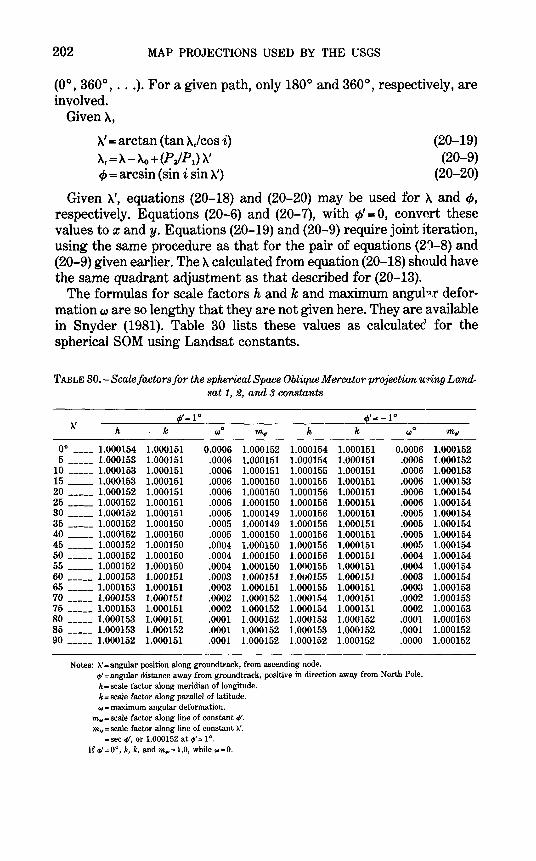
202 MAP PROJECTIONS USED BY THE USGS
(0°, 360°, ... ). For a given path, only 180° and 360°, respectively, are involved. Given~'
~'=arctan (tan ~/cos i) (20-19) A,=~-'Ao+(Pz/P1) ~' (20-9) q, =arcsin (sin i sin A') (20-20)
Given ~', equations (20-18) and (20-20) may be used for ~ and q,, respectively. Equations (20-6) and (20-7), with q,' = 0, convert these values to x andy. Equations (20-19) and (20-9) require joint iteration, using the same procedure as that for the pair of equations (21-8) and (20-9) given earlier. The ~ calculated from equation (20-18) should have the same quadrant adjustment as that described for (20-13).
The formulas for scale factors h and k and maximum angul ':l,f deformation w are so lengthy that they are not given here. They are available in Snyder (1981). Table 30 lists these values as calculated for the spherical SOM using Landsat constants.
TABLE 30.-Scale factors for the spherical Space Oblique Mercator pro}ection u!'ling Land-sat 1, 2, and 3 constants
)..' 41'= 10 41'=-10
k k "'0 m., h k "'0
0° ---- 1.000154 1.000151 0.0006 1.000152 1.000154 1.000151 0.0006 5 ----- 1.000153 1.000151 .0006 1.000151 1.000154 1.000151 .0006
10 ----- 1.000153 1.000151 .0006 1.000151 1.000155 1.000151 .0006 15 ----- 1.000153 1.000151 .0006 1.000150 1.000155 1.000151 .0006 20 ----- 1.000152 1.000151 .0006 1.000150 1.000156 1.000151 .0006 25 ----- 1.000152 1.000151 .0006 1.000150 1.000156 1.000151 .0006 30 ----- 1.000152 1.000151 .0005 1.000149 1.000156 1.000151 .0005 35 ----- 1.000152 1.000150 .0005 1.000149 1.000156 1.000151 .0005 40 ----- 1.000152 1.000150 .0005 1.000150 1.000156 1.000151 .0005 45 ----- 1.000152 1.000150 .0004 1.000150 1.000156 1.000151 .0005 50 ----- 1.000152 1.000150 .0004 1.000150 1.000156 1.000151 .0004 55 ----- 1.000152 1.000150 .0004 1.000150 1.000155 1.000151 .0004 60 ----- 1.000153 1.000151 .0003 1.000151 l.OU0155 1.000151 .0003 65 ----- 1.000153 1.000151 .0003 1.000151 1.000155 1.000151 .0003 70 ----- 1.000153 1.000151 .0002 1.000152 1.000154 1.000151 .0002 75 ----- 1.000153 1.000151 .0002 1.000152 1.000154 1.000151 .0002 80 ----- 1.000153 1.000151 .0001 1.000152 1.000153 1.000152 .0001 85 ----- 1.000153 1.000152 .0001 1.000152 1.000153 1.000152 .0001 90 ----- 1.000152 1.000151 .0001 1.000152 1.000152 1.000152 .0000
Notes: >.'=angular position along ground track, from ascending node. oil'=angular distance away from groundtrack, positive in direction away from North Pole. h= scale factor along meridian of longitude. k = scale factor along parallel of latitude. w =maximum angular deformation.
m.,= scale factor along line of constant oil'. m., =scale factor along line of constant }..'.
=sec oil', or 1.000152 at oil'= 1°. If .P'=0°, h, k, and m.,=l.O, while w=O.
m.,
1.000152 1.000152 1.000153 1.000153 1.000154 1.000154 1.000154 1.000154 1.000154 1.000154 1.000154 1.000154 1.000154 1.000153 1.000153 1.000153 1.000153 1.000152 1.000152
SPACE MAP PROJECTIONS 203
FORMULAS FOR THE ELLIPSOID
Since the SOM is intended to be used only for the rrapping of relatively narrow strips, it is highly recommended that the ellipsoidal form be used to take advantage of the high accuracy of scalE: available, especially as the imagery is further developed and used for more precise measurement. In addition to the normal modificati 'lns to the above spherical formulas for ellipsoidal equivalents, an add::tional element is introduced by the fact that Landsat is designed to sc8.n vertically, rather than in a geocentric direction. Therefore, "pseudotransformed" latitude (j>" and longitude }.." have been introduced. T'--~y relate to a geocentric groundtrack for an orbit in a plane through the center of the Earth. The regular transformed coordinates (j>' and }..' are related to the actual vertical groundtrack. The two groundtracks are only a maximum of 0.008° apart, although a lengthwise displacement of 0.028° for a given position may occur.
In addition, the following formulas accommodate a slight eilipticity in the satellite orbit. They provide a true-to-scale groundtrack £1r an orbit of any eccentricity, if the orbital motion follows Kepler's laws for twobodied systems, but the areas scanned by the satellite as she ·wn on the map are distorted beyond the accuracy desired if the eccentricity of the orbit exceeds about 0.05, well above the maximum reported eccentricity of Landsat orbits (about 0.002). For greater eccentricities, more complex formulas (Snyder, 1981) are recommended. If the orbital eccentricity is made zero, these formulas readily reduce to thos~ for a circular orbit. If the eccentricity of the ellipsoid is made zero, the formulas further reduce to the spherical formulas above. These forn1ulas vary slightly, but not significantly, from those previously publishei. In practice, the coordinates for each picture element (pixel) should not be calculated because of computer time required. Linear interpolation between occasional calculated points can be developed with ad~quate accuracy.
For the forward formulas, given a, e, i, P2, Pu ~'a!, e, -y, (j>, and 'A., find x and y. As with the spherical formulas, the X axis passes through each ascending and descending node, x increasing in the direction of satellite motion, and the Y axis intersects perpendicularly at the ascending node for the time t=O. Defining terms,
a, e= semimajor axis and eccentricity of ellipsoid, respectivE'1y (as for other ellipsoidal projections).
a', e = semimajor axis and eccentricity of satellite orbit, resp~ctively. -y = longitude of the perigee relative to the ascending node (for a
circular orbit, with e = 0, 1' is not involved).
204 MAP PROJECTIONS USED BY THE USGS
i, P 1, P 1, Ao, cp, A are as defined for the spherical SOM formulr~. For constants applying to the entire map:
B.= [1/(27r)JI:[(HJ -Sl)/(Jl +Sl)t'2]dA"
B2=[11(27r)]f ~1r[S(H +J)/{J2+S2)112]dA"
An= [11(7rn)]i:[(HJ -S1)/(J1 +82)1'2] cos nA"dA"
A~=[11(7rn)]i:[(HJ -S2)/(J2+S2)1'2] sin nA"dA" en= [1/(7rn)]i:[S(H +J)I(J2 +82)1'2] cos nA"dA" C'n = [1/(7rn)]i:[S(H +J)I(J2 +82)1'2] sin nA"dA" J =(1-e2
)3
W = [(1- e2 cos1 i)2/{1- e2)1] -1
Q = & sin2 i/(1- e1)
T = & sin1 i (2- e1)/(1- e1)1
H. =B.I(B11+B12)tn s. =B1/(B11+B11)111 in=(ll1r)!:cp" sin nA'dA' j,. = {l/7r}!:cp" cos nA'dA'
mn=(1/7r}!:(A" -A~ sin nA'dA' m~=(117r}!;1r(A" -A~ cos nA'dA'
(20-21)
(20-22) (20-23)
(20-24)
(20-25)
(20-26) (20-27) (20-28) (20-29) (20-30) (20-31) (20-32) (20-33)
(20-34)
(20-35) (20-36)
where cp" and A" are determined in these last four equations for the ground track as functions of A', from equations (20-40a), (20-60), (20-59), (20-58), (20-61), and (20-45) through (20-49).
To calculate An, A~, Bn1 en, and a,., the following functions, Yarying with A", are used:
S = (PiP.)L' sin i cos A" {(1 + T sin1 A")/[(1 + W sin1 A") (1 + Q sin1 A")]} 111 (20-37)
H= . . PiP. cost [ 1+Qsin1A" ] 1
'1 [ 1+ Wsin1A" , ·]
1+ w Sln1 A" (1+Q Sin1 A")1 ( )L
L' = (1- e cos E')1/{1- e1)111
E' = 2 arctan {tan 1/2(A"- -y) [(1- e)/(1 + e)]111)
(20-38)
(20-39) (20-40)
These constants may be determined from numerical integraf,')n, using Simpson's rule with 9° intervals. For noncircular orbits, i'ltegration must occur through the 360° or 21r cycle, as indicated. Many more terms are needed than for circular orbits.
For circular orbits, A~, B1, 0,., An if n is odd, en if n is even, Su in', mn', in if n is even, and mn if n is odd are all zero, while H 1 and L' are both 1.0. Numerical integration for the nonzero values of all the rer:~aining coefficients for circular orbits may be carried out from 0 to 1r/2, multiplying the result by 4.
SPACE MAP PROJECTIONS
To find x and y from cp and A.:
xla=xH1 +y'Sl yla=y'H~-xSt
where n n n
205
(20-41) (20-42)
x = B1A." +];. An sin nA."-];. A~ cos nA." +];. A~- [S/(J2 + 8 2)
112] ( 20_43)
In tan ( 1rl 4 + cp" /2) n n n
y'=l?}"+~ Cn sin nA."-~ C'n cos nA."+~ C,.+[JI(J2+S2)1'2] (20-44)
In tah \ 1rl 4 + cp" /2)
A."= arctan [cos i tan A.,+ (1- e2) sin i tan cp/cos A,]
A.,= A.- Ao +(PiP 1) (L + 'Y) L=E'-e' sinE' E' = 2 arctan {tan 112 (A."- 'Y) [(1- e')/(1 + e')]1'2} cp" =arcsin ([(1- e2
) cos i sin cp- sin i cos cp sin A.,]/ (1- e2sin2 c/>) 112
}
>-.o= 128.87° -(360°/251)p (Landsat 1, 2, 3 only)
(20-45) (20-46) (20-47) (20-48)
(20-49) (20-11)
Function E' is called the "eccentric anomaly'' along the orbit, and L is the "mean anomaly" or mean longitude of the satellite measur~d from perigee and directly proportional to time.
Equations (20-45) through (20-48) are solved by special iteration as described for equations (20-8) and (20-9) in the spherical form1.das, except that A." replaces A.', and each trial A." is placed in (20-48), fro~ which E' is calculated, then L from (20-4 7), A., from (20-46), and another trial A." from (20-45). This cycle is repeated until A." changes by less than the selected convergence. The last value of A., found is then used in (20-49) to find cp".
For circular orbits, in calculating x and y from cp and A., equations (20-41), (20-42), (20-47), and (20-48) may be eliminated, and equations (20-43) and (20-44) may be rewritten as follows:
xla=BtA."+A2 sin 2A."+A4 sin 4A."+ ... -[S/(J2 +S2)
112]
In tan ( 1rl 4 + cp" /2) yla= C1 sin A."+ C3 sin 3A." + ... + [JI(J2 +82
)112
]
In tan ( 1rl 4 + cp" /2)
(20-43a)
(20-44a)
Also, for circular orbits, (L + 'Y) in (20-46) is replaced by A.", and the two equations (20-45) and (20-46) are iterated together as were (20-8) and (20-9). Equation (20-49) is unchanged. For both circular and noncircular orbits, equation (20-37) is used to find S for the giv~n A." in equations (20-43), (20-44), (20-43a), and (20-44a).
206 MAP PROJECTIONS USED BY THE USGS
The closed forms of equations (20-43) and (20-44) are given below, but the repeated numerical integration necessitates replacem~nt by the series forms.
x = I 0X"[(HJ _ 82)/(J2 + 82)112] dA" _ [8/(J2 + 82)112] In tan (7r/4+ ¢"/2)
y' = I 0X"[8(H + J)/(J2 + 82)112] d>.." + [J/(J2 + 82)112] In tan ( 1rl 4 + ¢" /2)
(20-43b)
(20-44b)
While the above equations are sufficient for plotting a graticule according to the SOM projection, it is also desirable to relate th~se points to the true vertical ground track. To find ¢" and >.." in terms of¢' and >..', the shift between these two sets of coordinates is so sllall it is equivalent to an adjustment, requiring only small Fourier cc ~fficients, and very lengthy calculations if they are not used. The use of Fourier series is therefore highly recommended, although the one-time calculation of coefficients is more difficult than the foregoing calculation of An, Bn, and Cn.
n n n
¢" = ¢' + E jn sin n>..' + E j"' cos n>..'- E jn' n=l n=l n=l n n n
'A"='A'+E m" sinn'A'+E m'" cosn>..'-E m~ n~ n~ n~
(20-50)
(20-51)
For the circular orbit, as outlined in discussing other Fourier constants,
¢"=¢'+jt sin'A'+j3 sin3'A'+ ... 'A"='A'+m2 sin 2'A'+m4 sin 4>..'+ ...
For >..' in terms of time t from the initial ascending node,
'A'= 'Y + 2 arctan {(tan 112 E1 [(1 + e')/(1- e')]1'2} E' = e sinE'+ Lo + 21rt/P 2 Lo=E~-e sinE~ E~ = -2 arctan (tan 1/2-y [(1- e')/(1 + e)]t'2}
(20-50a) (20-51a)
(20-52) (20-53) (20-54) (20-55)
Equation (20-53) requires iteration, converging rapidly by suhstituting an initial trial E'=L0 +27rtiP2 in the right side, finding a new E' on the left, substituting it on the right, etc., until sufficient convergence occurs. For a circular orbit, >..' is merely 21rt/P2 •
The equations for functions of the satellite groundtrack, both forward and inverse, are given here, since some are used in calculating j" and mn as well. In any case a, e, i, P2, PH 'Ao, a', e, and 'Y must be given. For >..' and >.., if ¢ is given:
>..'=arcsin (sin ¢.fsin i) ¢. = ¢- arcsin {a& sin ¢ cos ¢/[Ro (1- e2 sin2 ¢ )112]} Ro=a! (1-e cosE1 E' = 2 arctan {tan 112 (>..' --y) [(1-e)/(1 +e)]112J
(20-56) (20-57) (20-58)
(20-40a)
SPACE MAP PROJECTIONS 207
where c/>11 is the geocentric latitude of the point geocentrically under the satellite, not the geocentric latitude corresponding to the vertical ground track latitude cp, and Ro is the radius vector to the satellite from the center of the Earth.
These equations are solved as a group by iteration, inserting a trial 'A'= arcsin (sin cp/sin i) in (20-40a), solving (20-58), (20-57), and (20-56) for a new 'A', etc. Each trial 'A' must be adjusted for quadrant .. , If the satellite is traveling north, add 360° times the number of orbits completed at the nearest ascending node (0, 1, 2, etc.). If traveling south, subtract 'A' from 360° times the number of orbits completec1 at the nearest descending node (1/2, 3/2, 5/2, etc.). For 'A,
'A = arctan [ (cos i sin 'A')/ cos 'A'] - (P ziP 1)(£ + 'Y) + 'Ao L = E'- e sinE'
using the 'A' and E' finally found just above.
(20-59) (20-60)
For a circular orbit, equations (20-58), (20-40a), and (20-60) are eliminated. Ro becomes the radius of the orbit (7,294,690 m for Landsat), and (L + 'Y) in (20-59) is replaced with 'A'. Iteration is eliminated as well.
If 'A of a point along the groundtrack is given, to find 'A' and cp,
'A'= arctan (tan 'A,/ cos i) 'At ='A- 'Ao+ (P1/P1) (L +-y)
(20-19) (20-46)
and L is found from (20-60) and (20-40a) above. The four equat!'lns are iterated as a group, as above, but the first trial 'A' and the quadrant adjustments should follow the procedures listed for equation (20.-8).
cp =arcsin (sin i sin 'A')+ arcsin { ae1 sin cp cos cp/ [Ro (1- e1 sin1 cp )111]) (20-61)
where Ro is determined from (20-58) and (20-40a), using the 'A' determined just above. Iteration is involved in (20-61), beginning with a trial cp of arcsin (sin i sin 'A').
For a circular orbit, only equations (20-19), (20-46), and (20-61) are involved, using 'A' in place of (L + 'Y) in (20-46) and using the. orbital radius for R0 • Iteration remains for calculations of both 'A' and cp.
If 'A' of a point along the groundtrack is given, cp is found from (20-61), (20-58), and (20-40a); while 'A is found from (20-59), (20-60), and (20-40a). For the circular orbit, (20-61) is sufficient for cp, and (20-59) provides 'A if 'A' is substituted for (L + 'Y ). Only (20-61) requires iteration for these calculations, whether the orbit is circular or noncircular.
Inverse formulas for the ellipsoidal form of the SOM projection, with an orbit of 0.05 eccentricity or less, follow: Given a, e, i, P1, P 1, 'Ao, a', e, -y, x, andy, to find cp and 'A, the general Fourier and other constants are
208 MAP PROJECTIONS USED BY THE USGS
first determined as described at the beginning of the forvrard equations. Then
A=A,-(P/Pt) (L +y)+Ao
where
(20-62)
A,= arctan (VI cos A.") (20-63) V = {[1- sin2 cJ>"/(1- e2)] cos i sin A"- sin i sin cJ>" [(1 + Q sin2 A.")
(1- sin2 cJ>")- U sin2 c/>"]112}1[1- sin2 4>" (1 + U)] (20-64) U = e2 cos2 i/( 1- e2) (20-65)
while L is found from (20-60), E' from (20-48), and A" and cJ>" from (20-68) and (20-69) below.
cJ> =arctan {(tan A" cos A,- cos i sin A,)/[(1- e2) sin i]}
If i = 0, equation (20-66) is indeterminate, but
(20-66)
cJ> =arcsin {sin cJ>"/[(1- e2)2 + e2 sin2 c/>"]112) (20-67)
No iteration is involved in equations (20-62) through (20-67), and the ATAN2 function of Fortran should be used with (20-63), but not (20-66), adding or subtracting 360° to or from A if necessary in (20-62) to place it between longs. 180° E. and W. For the circular orb~t, (20-48) and (20-60) do not apply, and (L + 'Y) in (20-62) is replaced with A" Other equations remain the same.
Iteration is required to find A" from x and y: n n n
A"= {x' + (SIJ) y'- .E [An+ (SIJ)Cn] sin n A."+ .E [A~+ (S/J)c,] r.os nA"- .E n=1 n=l n=1
[A~+ (S/J)C,]J/[B1 + (SIJ)B2 ] (20-68)
using equations (20-37), (20-70), (20-71), and various const<.nts. Iteration involves substitution of a trial A"= x'IB1 in the right side:, finding a new A." on the left side, etc.
For cJ>", the A." just calculated is used in the following equation:
In tan (7rl4+cJ>"/2)=(1+S2/J2)112(y'-B2 A."-E en sin n A."+E n=1 n=l
where
x' = (xla) H1- (yla)St y' = (y/a) H1 + (xla)St
C'n cos n A."- E C'n) n=1
(20-69)
(20-70) (20-71)
For the circular orbit, equations (20-70) and (20-71) are eliminated, and (20-68) and (20-69) are rewritten thus:
A."=[xla+(SIJ)(yla)-A2 sin 2 A"-A4 sin 4 A." - (S/J)(Ct sin A"+ CJ sin 3 A.")]/B1 (20-68a)
SPACE MAP PROJECTIONS 209
(20-69a)
The first is solved by iteration just as (20-68), using an initial>.."= xlaB1. The closed forms of equations (20-68), (20-69), (20-68a), and
(20-69a) involve both iteration and repeated numerical integration and are impractical:
'J! + (SIJ)y' = I f[(HJ _ sz)J(Jz + sz)tll]d >.." + (S/J) Ins<n +J)I(J2 +S2
)112Jd >.." (20-68b)
ln tan ('n·/4 + ¢"/2) = [1 + (S/J)2]
112[y'- I~" [S(H +J)I (J2 + S2) 112]d >.."} (20-69b)
(For the circular orbit, 'J! andy' are replaced by (x/a) and (y!a), respectively.)
For ¢' and >: in terms of cJ>" and >..", the same Fourier series developed for equations (20-50) and (20-51) may be used with reversal of signs, since the correction is so small. That is,
¢' = <!>"- E j,. sin n >.."- E l,. cos n >.." + E l,. (20-72) n=l n=l n=l
>..' = >.."- E m,. sin n >.."- t m',. cos n >.." + E m',. n=l n=l n=l
(20-73)
Equations (20-72) and (20-73) are, of course, not the exact inverses of (20-50) and (20-51), although the correct coefficients may 1:-~ derived by an analogous numerical integration in terms of >..", rather than >..'. The inverse values of ¢' and >..' from (20-72) and (20-73) z.re within 0.000003° and 0.000009°, respectively, of the true inverses of (20-50) and (20-51) for the Landsat orbit.
For the circular orbit, as before, equations (20-72) an-i (20-73) simplify to the following:
<!>' = ¢"-J1 sin >.."- j3 sin 3 >.."- . . . >..' = >:'- m2 sin 2 >.."- m4 sin 4 >.."- ...
(20-72a) (20-73a)
The following values of Fourier coefficients for the ellips<''dal SOM are listed for Landsat orbits, using the Clarke 1866 ellipsoid (a= 6,378,206.4 m and e1 = 0.00676866) and a circular orbit (R=7,294,690 m, i=99.092°, P 2/P1 =18/251):
B1 = 1.005798138 for >.." in radians = 0.0175544891 for>.." in degrees
A 1 = - 0.0010979201 A4= -0.0000012928 A6 = - 0.0000000021 cl = o.1434409899 C3= 0.0000285091 C5 = -0.0000000011
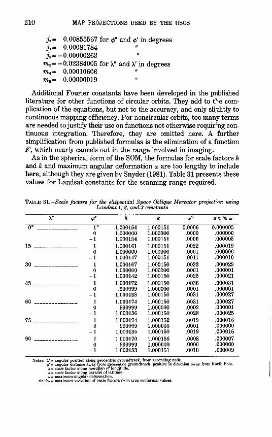
210 MAP PROJECTIONS USED BY THE USGS
J·· = 0.00855567 for cp" and cp' in degrees J~ = 0.00081784 " is= - 0.00000263 " ~ = - 0.02384005 for >.." and >..' in degrees m4 = 0.00010606 " m6 = 0.00000019 "
Additional Fourier constants have been developed in the published literature for other functions of circular orbits. They add to t~e complication of the equations, but not to the accuracy, and only slirrhtly to continuous mapping efficiency. For noncircular orbits, too many terms are needed to justify their use on functions not otherwise requir:ng continuous integration. Therefore, they are omitted here. A further simplification from published formulas is the elimination of a function F, which nearly cancels out in the range involved in imaging.
As in the spherical form of the SOM, the formulas for scale factors h and k and maximum angular deformation w are too lengthy to include here, although they are given by Snyder (1981). Table 31 presents these values for Landsat constants for the scanning range required.
TABLE 31.-Scale factors for the ellipsoidal Space Oblique Mercator project·:()n using Landsat 1, 2, and 3 constants
'A" .P" h k wo 8:'1 1/2 w
oo -------------- 10 1.000154 1.000151 0.0006 0.000005 0 1.000000 1.000000 .0000 .000000
-1 1.000154 1.000151 .0006 .000005
15 --------------- 1 1.000161 1.000151 .0022 .000019 0 1.000000 1.000000 .0001 .000000
-1 1.000147 1.000151 .0011 .000010
30 --------------- 1 1.000167 1.000150 .0033 .000029 0 1.000000 1.000000 .0001 .000001
-1 1.000142 1.000150 .0025 .000021
45 --------------- 1 1.000172 1.000150 .0036 .000031 0 .999999 1.000000 .0001 .000001
-1 1.000138 1.000150 .0031 .000027
60 --------------- 1 1.000174 1.000150 .0031 .000027 0 .999999 1.000000 .0002 .000001
-1 1.000136 1.000150 .0028 .000025
75 --------------- 1 1.000174 1.000152 .0019 .000016 0 .999999 1.000000 .0001 .000000
-1 1.000135 1.000150 .0019 .000016
90 --------------- 1 1.000170 1.000156 .0008 .000007 0 .999999 1.000000 .0000 .000000
-1 1.000133 1.000151 .0010 .000009
Notes: 'A"= angular position along ~eocentric groundtrack, from ascendin~ node. tJ>"= anEiar aistance away rom ~eocentric groundtrack, positive m direction away from North Pole. h= sc e factor along meridian o longitude. k= scale factor along parallel of latitude. w= maximum angular deformation.
sin Vzw= maximum variation of scale factors from true conformal values.
MISCELLANEOUS MAP PROJECTIONS
Only two map projections described in this study cannot b~ satisfactorily placed in one of the four categories previously listed. If this study included many of the projections not used by the USGS, several additional categories would be shown, and those projections di~cussed below would be placed with similar projections and' probably r~~moved from the "miscellaneous" classification.
21. VAN DER GRINTEN PROJECTION
SUMMARY
• Neither equal-area nor conformal. • Shows entire globe enclosed in a circle. • Central meridian and Equator are straight lines. • All other meridians and parallels are arcs of circles. • A curved modification of the Mercator projection, with great distortion in the polar
areas. • Equator is true to scale. • Used for world maps. • Used only in the spherical form. • Presented by van der Grinten in 1904.
HISTORY, FEATURES, AND USAGE
In a 1904 issue of a German geographical journal, Alphons J. van der Grinten (1852-?) of Chicago presented four projections showing the entire Earth. Aside from having a straight Equator and central meridian, three of the projections consist of arcs of circles for meridig.ns and parallels; the other projection has straight-line parallels. The projec-
, tions are neither conformal nor equal-area (van der Grinten, 1904; 1905). They were patented in the United States by van der Grinten in 1904.
The best-known Vander Grinten projection, his first (fig. 30), shows the world in a circle and was invented in 1898. It is designed fo:-:- use in the spherical form only. There are no special features to preserve in an ellipsoidal form. It has been used by the National Geographic Society for their standard world map since 1943, printed at various scaJes and with the central meridian either through America or along the Greenwich meridian; this use has prompted others to employ the projection. The USGS has used one of the National Geographic maps as a r~se for a four-sheet set of maps of World Subsea Mineral Resources, 1970, one at a scale of 1:60,000,000 and three at 1:39,283,200 (a scale usee by the National Geographic), and for three smaller maps in the National Atlas
~11
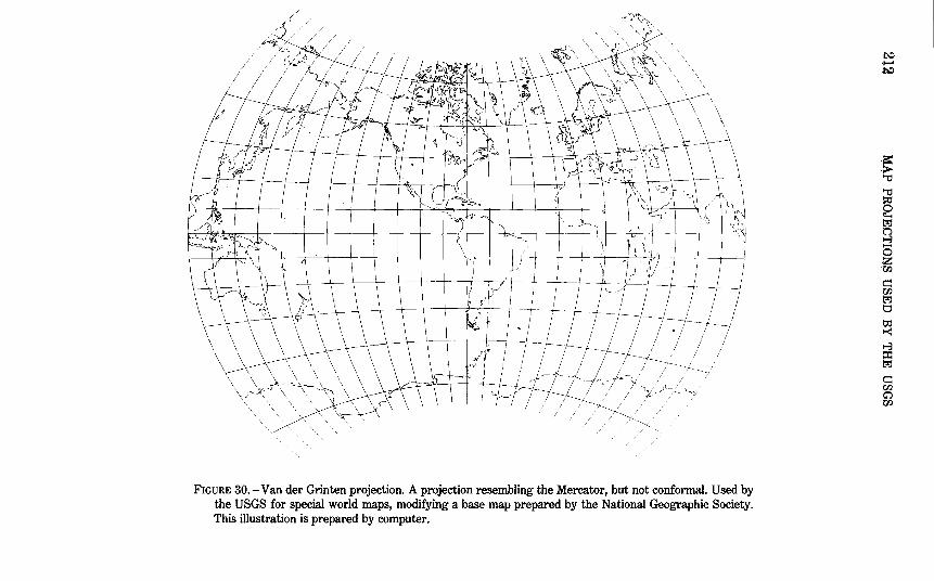
FIGURE 30.-Vander Grinten projection. A projection resembling the Mercator, but not conformal. Used by the USGS for special world maps, modifying a base map prepared by the National Geographic Society. This illustration is prepared by computer.
~ -~ .~
~ ;g <0 [;3 D :j 0 z 00
~ 00 t_:r;j t::1
~ 1-3 :I: t_:r;j
~ 00 c;1 00
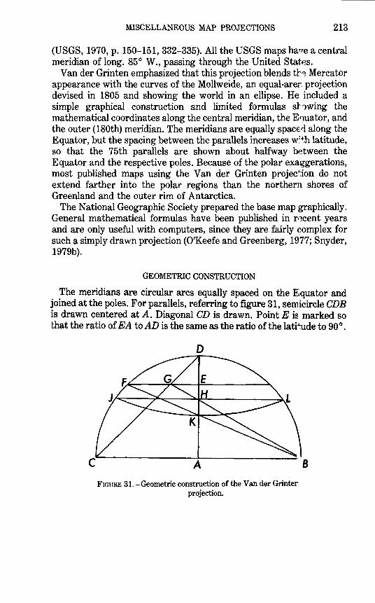
MISCELLANEOUS MAP PROJECTIONS 213
(USGS, 1970, p. 150-151, 332-335). All the USGS maps ha-rre a central meridian of long. 85° W., passing through the United States.
Van der Grinten emphasized that this projection blends tr~ Mercator appearance with the curves of the Mollweide, an equal-arer. projection devised in 1805 and showing the world in an ellipse. He included a simple graphical construction and limited formulas sl''lWing the mathematical coordinates along the central meridian, the E~uator, and the outer (180th) meridian. The meridians are equally space:<! along the Equator, but the spacing between the parallels increases w:~h latitude, so that the 75th parallels are shown about halfway between the Equator and the respective poles. Because of the polar exaggerations, most published maps using the Van der Grinten projection do not extend farther into the polar regions than the northern shores of Greenland and the outer rim of Antarctica.
The National Geographic Society prepared the base map graphically. General mathematical formulas have been published in rr~cent years and are only useful with computers, since they are fairly complex for such a simply drawn projection (O'Keefe and Greenberg, 1977; Snyder, 1979b).
GEOMETRIC CONSTRUCTION
The meridians are circular arcs equally spaced on the Equator and joined at the poles. For parallels, referring to figure 31, semicircle CDB is drawn centered at A. Diagonal CD is drawn. Point E is marked so that the ratio of EA to AD is the same as the ratio of the lati~ude to 90°.
D
FIGURE 31. -Geometric construction of the Van der Grinter projection.
B

214 MAP PROJECTIONS USED BY THE USGS
Line FE is drawn parallel to CB, and FB and GB are connected. At H, the intersection of GB and AD, JHL is drawn parallel to CB. A c~rcular arc, representing the parallel of latitude, is then drawn througl' JKL.
FORMULAS FOR THE SPHERE
The general formulas published are in two forms. Both sets giv~ identical results, but the 1979 formulas are somewhat shorter and are given here with some rearrangement and addition of new inverse equations. For the forward calculations, given R, Ao, cp, and A (giving tru~ scale along the Equator), to find x andy:
X=± rR [A(G-P2)+[A2(G-P2)
2 -(P2 +A2)(G2 -P2))1'2}/(P2 +A2) (21-1)
taking the sign of (A-Ao). Note that (A-Ao) must fall between +180° and -180°; if necessary, 360° must be added or subtracted. The X axis lies along the Equator, x increasing easterly, while theY axis coincides with the central meridian Ao·
y= ±rR{ PQ-A[(A 2 + l)(P2 +A2)-Q2]112 }/(P2 +A 2)
taking the sign of cp,
where A= 1/2lri(A- Ao)- (A- Ao)l 1rl G=cos 8/(sin 8+cos 8-1) P= G(2/sin 8-1) 8 = arcsin l2cp/ 1r I Q=A2+G
(21-2)
(21-3) (21-4) (21-5) (21-6) (21-6a)
But if cp = 0 or A= Ao, these equations are indeterminant. In that case, if c/>=0,
(21-7)
and
x=O
and
y = ± rR tan (8/2) (21-8)
taking the sign of cp. It may be noted that absolute values (syml''ll I I> are used in several cases. The origin is at the center (c/>=0, A=X").
For the inverse equations, given R, Ao, x, and y, to find cp and A: Because of the complications involved, the equations are given in the
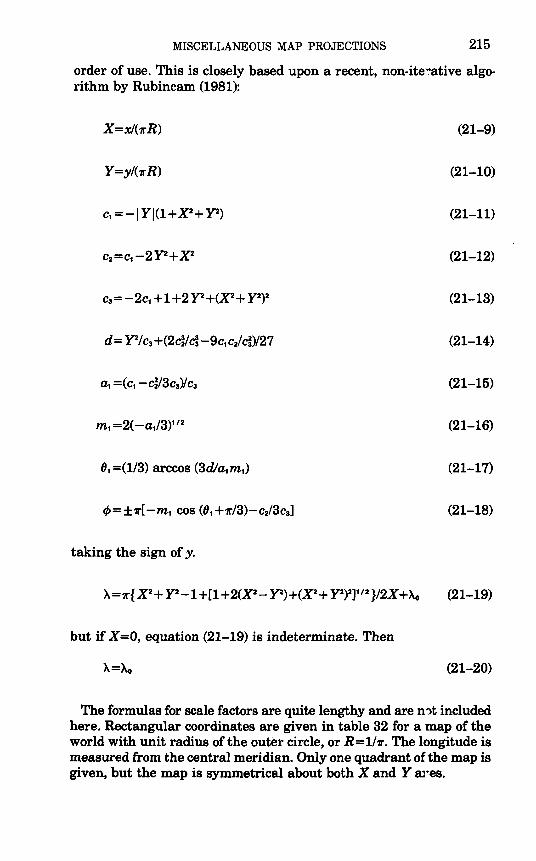
MISCELLANEOUS MAP PROJECTIONS 215
order of use. This is closely based upon a recent, non-ite~ative algorithm by Rubincam (1981):
X=xl(-rrR) (21-9)
Y=yl(-rrR) (21-10)
(21-11)
(21-12)
(21-13)
(21-14)
(21-15)
(21-16)
(21-17)
4>= ±-rr[ -m1 cos (()1 +-rr/3)-ci3cal (21-18)
taking the sign of y.
(21-19)
but if X=O, equation (21-19) is indeterminate. Then
A.=A.o (21-20)
The formulas for scale factors are quite lengthy and are n'lt included here. Rectangular coordinates are given in table 32 for a map of the world with unit radius of the outer circle, or R=ll-rr. The longitude is measured from the central meridian. Only one quadrant of the map is given, but the map is symmetrical about both X and Y ar:es.
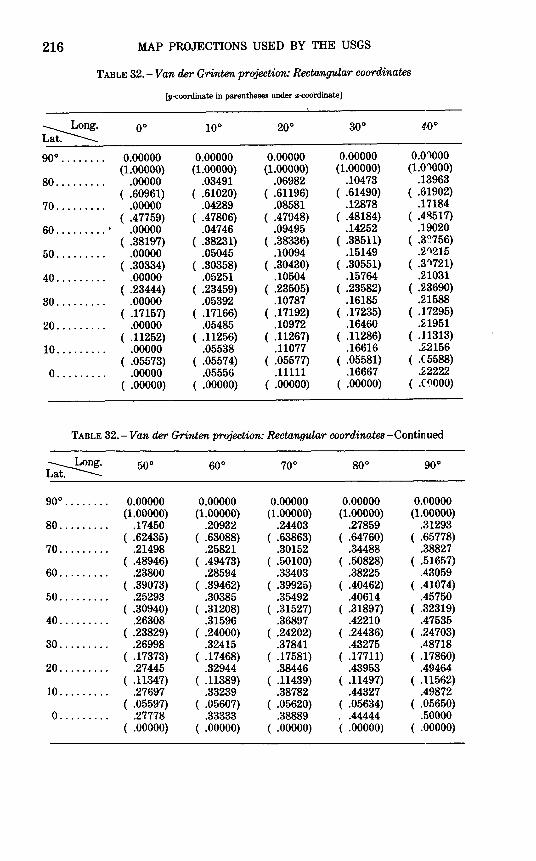
216 MAP PROJECTIONS USED BY THE USGS
TABLE 32.- Vander Grinten projection: Rectangular coordinates
(y-coordinate in parentheses under x-coordinate]
~ oo 100 20° 30° 40° L .
90° ........ 0.00000 0.00000 0.00000 0.00000 0.01000 (1.00000) (1.00000) (1.00000) (1.00000) (1.01000)
80 ......... .00000 .03491 .06982 .10473 .13963 ( .60961) ( .61020) ( .61196) ( .61490) ( .61902)
70 ......... .00000 .04289 .08581 .12878 .17184 ( .47759) ( .47806) ( .47948) ( .48184) ( .4~517)
60 ......... ' .00000 .04746 .09495 .14252 .19020 ( .38197) ( .38231) ( .38336) ( .38511) ( .3~756)
50 ......... .00000 .05045 .10094 .15149 .2/1215 ( .30334) ( .30358) ( .30430) ( .30551) ( .3"1721)
40 ......... .00000 .05251 .10504 .15764 .2.1031 ( .23444) ( .23459) ( .23505) ( .23582) ( .2.3690)
30 ......... .00000 .05392 .10787 .16185 .2.1588 ( .17157) ( .17166) ( .17192) ( .17235) ( .17295)
20 ......... .00000 .05485 .10972 .16460 .2.1951 ( .11252) ( .11256) ( .11267) ( .11286) ( .11313)
10 ......... .00000 .05538 .11077 .16616 .2.2156 ( .05573) ( .05574) ( .05577) ( .05581) ( .(]5588)
0 ......... .00000 .05556 .11111 .16667 .2.2222 ( .00000) ( .00000) ( .00000) ( .00000) ( .(~000)
TABLE 32.- Vander Grinten projection: Rectangular coordinates-Continued
~ Lat. 50° 60° 70° goo 90°
90° ........ 0.00000 0.00000 0.00000 0.00000 0.00000 (1.00000) (1.00000) (1.00000) (1.00000) (1.00000)
80 ......... .17450 .20932 .24403 .27859 .31293 ( .62435) ( .63088) ( .63863) ( .64760) ( .65778)
70 ......... .21498 .25821 .30152 .34488 .38827 ( .48946) ( .49473) ( .50100) ( .50828) ( .51657)
60 ......... .23800 .28594 .33403 .38225 .43059 ( .39073) ( .39462) ( .39925) ( .40462) ( .41074)
50 ......... .25293 .30385 .35492 .40614 .45750 ( .30940) ( .31208) ( .31527) ( .31897) ( .32319)
40 ......... .26308 .31596 .36897 .42210 .47535 ( .23829) ( .24000) ( .24202) ( .24436) ( .24703)
30 ......... .26998 .32415 .37841 .43275 .48718 ( .17373) ( .17468) ( .17581) ( .17711) ( .17860)
20 ......... .27445 .32944 .38446 .43953 .49464 ( .11347) ( .11389) ( .11439) ( .11497) ( .11562)
10 ......... .27697 .33239 .38782 .44327 .49872 ( .05597) ( .05607) ( .05620) ( .05634) ( .05650)
0 ......... .27778 .33333 .38889 .. 44444 .50000 ( .00000) ( .00000) ( .00000) ( .00000) ( .00000)
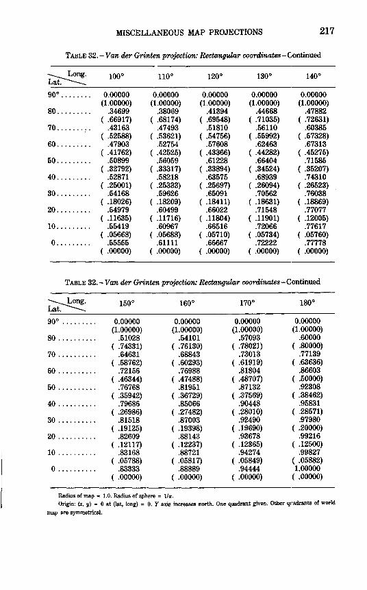
MISCELLANEOUS MAP PROJECTIONS 217
TABLE 32.- Vander Grinten projection: Rectangular coordinates-Continued
~ 100° 110° 120° 130° 140° . 90° ........ 0.00000 0.00000 0.00000 0.00000 0.00000
(1.00000) (1.00000) (1.00000) (1.00000) (1.00000) 80 ......... .34699 .38069 .41394 .44668 .47882
( .66917) ( .68174) ( .69548) ( .71035) ( .72631) 70 ......... .43163 .47493 .51810 .56110 .60385
( .52588) ( .53621) ( .54756) ( .55992) ( .57328) 60 ......... .47903 .52754 .57608 .62463 .67313
( .41762) ( .42525) ( .43366) ( .44282) ( .45275) 50 ......... .50899 .56059 .61228 .66404 .71585
( .32792) ( .33317) ( .33894) ( .34524) ( .35207) 40 ......... .52871 .58218 .63575 .68939 .74310
( .25001) ( .25333) ( .25697) ( .26094) ( .26523) 30 ......... .54168 .59626 .65091 .70562 .76038
( .18026) ( .18209) ( .18411) ( .18631) ( .18869) 20 ......... .54979 .60499 .66022 .71548 .77077
( .11635) ( .11716) ( .11804) ( .11901) ( .12005) 10 ......... .55419 .60967 .66516 .72066 .77617
( .05668) ( .05688) ( .05710) ( .05734) ( .05760) 0 ......... .55555 .61111 .66667 .72222 .77778
( .00000) ( .00000) ( .00000) ( .00000) ( .00000)
TABLE 32.-Vander Grinten projection: Rectangular coordinates-Continued
~ 150° 160° 170° 180° Lat.
90° ......... 0.00000 0.00000 0.00000 0.00000 (1.00000) (1.00000) (1.00000) (1.00000)
80 .......... .51028 .54101 .57093 .60000 ( .74331) ( .76130) ( .78021) ( .80000)
70 .......... .64631 .68843 .73013 .77139 ( .58762) ( .60293) ( .61919) ( .63636)
60 .......... .72156 .76988 .81804 .86603 ( .46344) ( .47488) ( .48707) ( .50000)
50 .......... .76768 .81951 .87132 .92308 ( .35942) ( .36729) ( .37569) ( .38462)
40 .......... .79686 .85066 .90448 .95831 ( .26986) ( .27482) ( .28010) ( .28571)
30 .......... .81518 .87003 .92490 .97980 ( .19125) ( .19398) ( .19690) ( .20000)
20 .......... .82609 .88143 .93678 .99216 ( .12117) ( .12237) ( .12365) ( .12500)
10 .......... .83168 .88721 .94274 .99827 ( .05788) ( .05817) ( .05849) ( .05882)
0 .......... .83333 .88889 .94444 1.00000 ( .00000) ( .00000) ( .00000) ( .00000)
Radius of map = 1.0. Radius of sphere = 11 .... Origin: (x, y) = 0 at (lat, long) = 0. Y axis increases north. One quadrant given. Other qt•adrants of world
map are symmetrical.

22. SINUSOIDAL PROJECTION
SUMMARY
• Pseudocylindrical projection. • Equal-area. • Central meridian is a straight line; all other meridians are shown as sinusoidal
curves. • Parallels are equally spaced straight lines. • Scale is true along central meridian and all parallels. • Used for world maps with single central meridian or in interrupt~d form with
several central meridians. • Used for maps of South America and Mrica. • Used since the mid-16th century.
HISTORY
There is an almost endless number of possible projections with horizontal straight lines for parallels of latitude and curve 1 lines for meridians. They are sometimes called pseudocylindrical because of their partial similarity to cylindrical projections. Scores of such projections have been presented, purporting various special advantages, although several are strikingly similar to other members of the group (Snyder, 1977). While there were rudimentary projections with straight parallels used as early as the 2nd century B.C. by Hipparchus, the first such projection still used for scientific mapping of th ~ sphere is the Sinusoidal.
This projection (fig. 32), used for world maps as well as maps of conti~ents and other regions, especially those bordering the E~·~1ator, has been given many names after various presumed originator~:' but it is most frequently called by the named used here. Among the first to show the Sinusoidal projection was Jean Cossin of Dieppe, who used it for a world map of 1570. In addition, it was used by Jodocus Hondius for maps of South America and Mrica in some of his editions of Mercator's atlases of 1606-1609. This is probably the basis for one of the names of the projection: The Mercator Equal-Area. Nicolas Sanson (1600-67) of France used it in about 1650 for maps of continonts, while John Flamsteed (1646-1719) of England later used it for rt,ar maps. Thus, the name usanson-Flamsteed" has often been appPed to the Sinusoidal projection, even though they were not the originators (Keuning, 1955, p. 24; Deetz and Adams, 1934, p. 161).
While maps ofNortli America are no longer drawn to the f:nusoidal, South America and Mrica are still shown on this projectior in recent Rand MeN ally atlases.
219
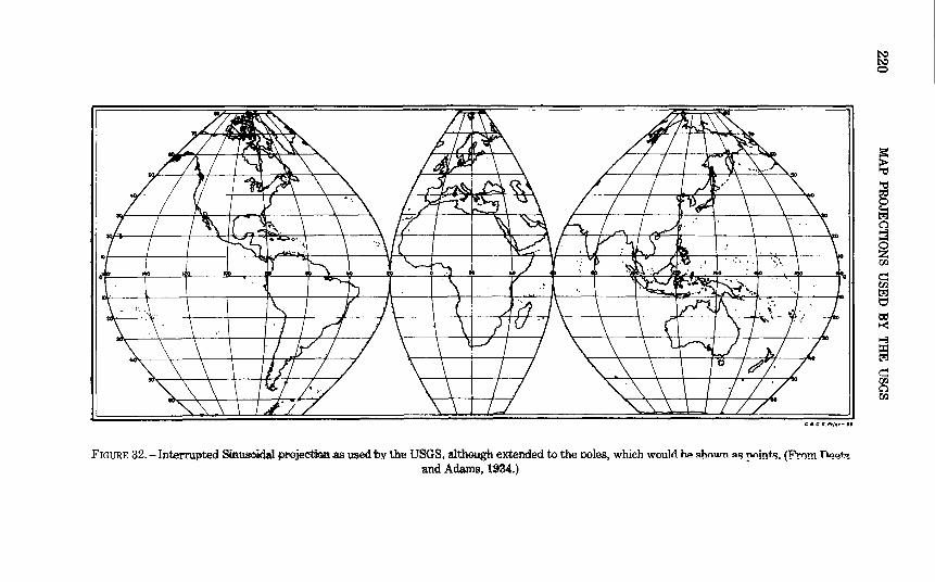
FIGURE 32.- Interrupted SinusOOdal projection .as used by the USGS. although extended to the noles, which would hP- "hown ~$J !'0int"l. {Fr()m n~~t~ and Adams, 1934.)
~ ~ 0
~
~ (j 1-3
~ 00
~ 00 t_::l:j t=' txl t-< 1-3
gj ~ 00 0 00
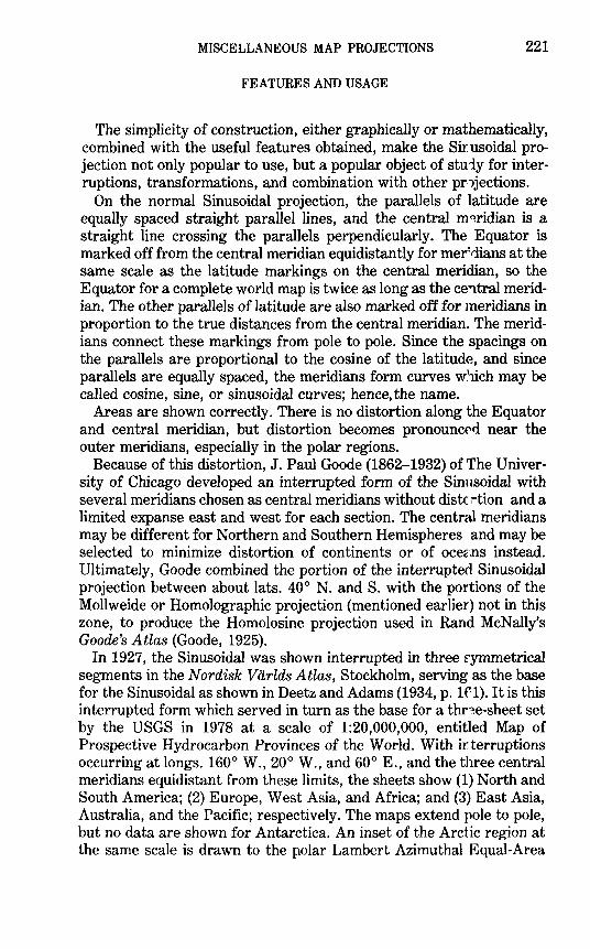
MISCELLANEOUS MAP PROJECTIONS 221
FEATURES AND USAGE
The simplicity of construction, either graphically or mathematically, combined with the useful features obtained, make the Sill usoidal projection not only popular to use, but a popular object of stuiy for interruptions, transformations, and combination with other pr,1jections.
On the normal Sinusoidal projection, the parallels of latitude are equally spaced straight parallel lines, and the central m~ridian is a straight line crossing the parallels perpendicularly. The Equator is marked off from the central meridian equidistantly for mer::dians at the same scale as the latitude markings on the central meridian, so the Equator for a complete world map is twice as long as the ce'l.tral meridian. The other parallels of latitude are also marked off for 1neridians in proportion to the true distances from the central meridian. The meridians connect these markings from pole to pole. Since the spacings on the parallels are proportional to the cosine of the latitude, and since parallels are equally spaced, the meridians form curves which may be called cosine, sine, or sinusoidal curves; hence, the name.
Areas are shown correctly. There is no distortion along the Equator and central meridian, but distortion becomes pronounc('d near the outer meridians, especially in the polar regions.
Because of this distortion, J. Paul Goode (1862-1932) of The University of Chicago developed an interrupted form of the Sinusoidal with several meridians chosen as central meridians without distc rtion and a limited expanse east and west for each section. The central meridians may be different for Northern and Southern Hemispheres and may be selected to minimize distortion of continents or of ocez.ns instead. Ultimately, Goode combined the portion of the interrupted Sinusoidal projection between about lats. 40° N. and S. with the portions of the Mollweide or Homolographic projection (mentioned earlier) not in this zone, to produce the Homolosine projection used in Rand McNally's Goode's Atlas (Goode, 1925).
In 1927, the Sinusoidal was shown interrupted in three Eymmetrical segments in the Nordisk Viirlds Atlas, Stockholm, serving as the base for the Sinusoidal as shown in Deetz and Adams (1934, p. 1f1). It is this interrupted form which served in turn as the base for a thr~e-sheet set by the USGS in 1978 at a scale of 1:20,000,000, entitled Map of Prospective Hydrocarbon Provinces of the World. With i:r:terruptions occurring at longs. 160° W., 20° W., and 60° E., and the three central meridians equidistant from these limits, the sheets show (1) North and South America; (2) Europe, West Asia, and Africa; and (3) East Asia, Australia, and the Pacific; respectively. The maps extend pole to pole, but no data are shown for Antarctica. An inset of the Arctic region at the same scale is drawn to the polar Lambert Azimuthal Equal-Area
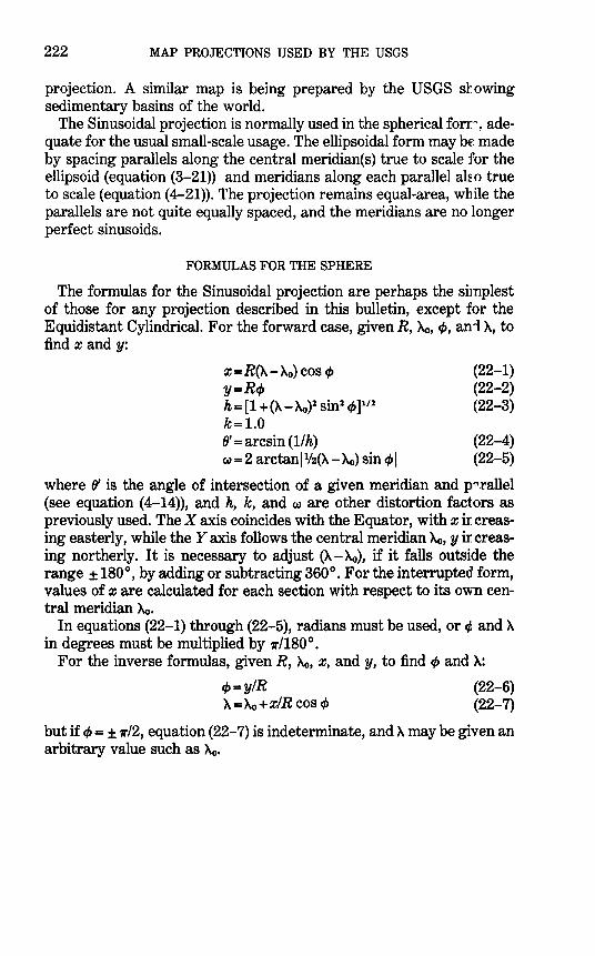
222 MAP PROJECTIONS USED BY THE USGS
projection. A similar map is being prepared by the USGS sb owing sedimentary basins of the world.
The Sinusoidal projection is normally used in the spherical form~ adequate for the usual small-scale usage. The ellipsoidal form may b~ made by spacing parallels along the central meridian(s) true to scale for the ellipsoid (equation (3-21)) and meridians along each parallel ale·o true to scale (equation (4-21)). The projection remains equal-area, while the parallels are not quite equally spaced, and the meridians are no longer perfect sinusoids.
FORMULASFORTHESPHERE
The formulas for the Sinusoidal projection are perhaps the si1nplest of those for any projection described in this bulletin, except for the Equidistant Cylindrical. For the forward case, given R, Ac,, ¢, ani X., to find x andy:
X=R(X.-Ac,) cos <I>
y=R<P h= [1 +(X.-Ac,)1 sin1 </>] 111
k=l.O 8' =arcsin (1/h) w = 2 arctan 11/z(X.- Ac,) sin <I> I
(22-1) (22-2) (22-3)
(22-4) (22-5)
where 8' is the angle of intersection of a given meridian and p~.rallel (see equation (4-14)), and h, k, and w are other distortion factors as previously used. The X axis coincides with the Equator, with x increasing easterly, while the Y axis follows the central meridian Ac,, y increasing northerly. It is necessary to adjust (A- Xo), if it falls outside the range ± 180°, by adding or subtracting 360°. For the interrupted form, values of x are calculated for each section with respect to its own central meridian Ac,.
In equations (22-1) through (22-5), radians must be used, or q. and A in degrees must be multiplied by 1rll80°.
For the inverse formulas, given R, Ac,, x, andy, to find <1> and X.:
<J>=yiR X.='Ao+xiR cos cp
(22-6) (22-7)
but if <1> = ± 1r/2, equation (22-7) is indeterminate, and X. may be given an arbitrary value such as Ao.
APPENDIXES

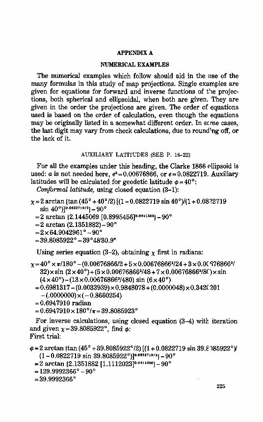
APPENDIX A
NUMERICAL EXAMPLES
The numerical examples which follow should aid in the use of the many formulas in this study of map projections. Single examples are given for equations for forward and inverse functions of t~e projections, both spherical and ellipsoidal, when both are given. They are given in the order the projections are given. The order of equations used is based on the order of calculation, even though the equations may be originally listed in a somewhat different order. In scme cases, the last digit may vary from check calculations, due to round:ng off, or the lack of it.
AUXILIARY LATITUDES (SEE P. 16-22)
For all the examples under this heading, the Clarke 1866 ellipsoid is used: a is not needed here, e1=0.00676866, or e=0.082271g. Auxiliary latitudes will be calculated for geodetic latitude c/>=40°:
Conformal latitude, using closed equation (3-1):
x=2 arctan {tan(45° +40°/2)[(1-0.082271g sin 40°)/(1 +0.08~271g sin 40o)]o.o8117191lJ _goo
= 2 arctan {2.144506g [0.8gg5456]0 ·0411360}-goo =2 arctan (2.1351882)-goo =2x64.g042g61 o -goo = 3g.8085g22 ° = 3g 0 48'30.g"
Using series equation (3-2}, obtaining x first in radians:
x=40° x 11'1180° -(0.00676866/2 + 5 x0.006768661/24+3 xO.OCf-)768663/ 32) X sin (2 X 40°) + (5 X 0.006768661/48 + 7 X 0.006768663/8('} X sin ( 4 X 40°)- (13 X 0.006768663/480) sin (6 X 40°)
=0.6g81317-(0.0033g3g)xO.g848078+(0.0000048)x0.342C201 - (.0000000) X (- 0.8660254)
=0.6g47g10 radian = 0.6g4 7g10 X 180° f1r = 3g.8085g23°
For inverse calculations, using closed equation (3-4) with iteration and given x=3g.8085g22°, find cp: First trial:
</>=2 arctan (tan (45° +3g.8085g22°/2) [(1 +0.082271g sin 3g.~'185g22°)/ (1- 0.082271g sin 3g.8085g22°)]0·08117191l)- goo
= 2 arctan (2.1351882 [1.1112023]0 ·0411360)- goo = 129.9992366°-90° = 3g. 9gg2366 °
225
226 MAP PROJECTIONS USED BY THE USGS
Second trial:
~=2 arctan {2.1351882 [(1+0.0822719 sin 39.9992366°)/(1-0.0°22719 sin 39.9992366°)]0
·0411360
}-90° =2 arctan (2.1445068)-90° =39.9999970°
The third trial gives ~=40.0000000°, also given by the fourth trial. Using series equation (3-5):
~ = 39.8085922° X 11"/180° + (0.00676866/2 + 5 X 0.006768662/24 + 0.006768663/12) sin (2 x 39.8085922°) + (7 x 0.006768662/48 + 29 X 0.006768663/240) sin (4 X 39.8085922°) + (7 X 0.006768663/120) sin (6x39.8085922°)
= 0.6947910 +(0.0033939)x 0.9836256 +(0.0000067) x 0.3545461 +(O.OOOOOOO)x( -0.8558300)
=0.6981317 radian = 0.6981317 X 180° /11" = 40.0000000°
Isometric latitude, using equation (3-7):
1P=ln {tan (45° +40°/2) [(1-0.0822719 sin 40°)/(1 +0.0822719 sin 40o)]o.o82271912J
= ln (2.1351882) =0.7585548
Using equation (3-8) with the value of x resulting from the ak'0ve examples:
1P=ln tan (45° +39.8085923°/2) = ln tan 64.9042962 ° =0.7585548
For inverse calculations, using equation (3-9) with 1P = 0. 75855-t8:
X= 2 arctan eo.7s8ss48- 90o =2 arctan (2.1351882)-90° = 39.8085922°
From this value of x, ~ may be found from (3-4) or (3-5) ae· shown above.
Using iterative equation (3-10), with 1P = 0. 7585548, to find ¢: First trial:
~=2 arctan eo.7s8ss48_90o = 39.8085922°, as just above.
Second trial:
~ =2 arctan {e0·7585548 [(1 +0.0822719 sin 39.8085922°)/(1-0.0822719
sin 39.8085922o)]o.o82271912J- 90o
APPENDIXES
=2 arctan (2.1351882x 1.0043469)-90° = 39.9992365 °
Third trial:
227
cp =2 arctan {e0 ·7585548 [(1 +0.0822719 sin 39.9992365°)/(1-0.0822719
sin 39.9992365°)]0•081171911
}-90° = 39.9999970°
Fourth trial, substituting 39.9999970° in place of 39.99923~'5°:
cp = 40.0000000 °, also given by fifth trial.
Authalic latitude, using equations (3-11) and (3-12):
q=(1-0.00676866) {sin 40°/(1-0.00676866 sin1 40°)-[1/(2 x 0.0822719)] ln [(1- 0.0822719 sin 40°)/(1 + 0.0822719 sin 40°)]}
= 0.9932313 (0.6445903- 6.077 4117 ln 0.8995456) =1.2792602
qp = (1- 0.00676866) {sin 90° /(1- 0.00676866 sin1 90°)- [1/ (2 x 0.0822719)] ln [(1- 0.0822719 sin 90°)/(1 + 0.0822719 sin 90°)]}
=1.9954814 {3 =arcsin (1.2792602/1.9954814)
=arcsin 0.6410785 =39.8722878° =39°52'20.2"
Determining {3 from series equation (3-14) involves the same pattern as the example for equation (3-5) given above.
For inverse calculations, using equation (3-17) with iter<:\.tive equation (3-16), given {3=39.8722878°, and qp=1.9954814 as determined above:
q= 1.9954814 sin 39.8722878° = 1.2792602
First trial:
cp =arcsin (1.2792602/2) =39.762435°
Second trial:
c/>=39.7642435° +(180°/11') {[(1-0.00676866 sin1 39.7642435°}1/(2 cos 39.7642435 °)] [1.2792602/(1- 0.00676866)- sin 39.7642435 ° I (1-0.00676866 sin1 39.7642435°) + [1/(2 x 0.0822719)] ln [(1- 0.0822719 Ein 39. 7642435°)/ (1 + 0.0822719 sin 39. 7642435°)]]}
= 39.9996014 °
228 MAP PROJECTIONS USED BY THE USGS
Third trial, substituting 39.9996014 o in place of 39.7642435°,
c/> = 39.9999992°
Fourth trial gives the same result. Finding cJ> from {3 by series equation (3-18) involves the same pattern
as the example for equation (3-5) given above. Rectifying latitude, using equations (3-20) and (3-21):
M = a[(1- 0.00676866/4-3 x 0.006768662/64-5 x 0.006768663/256>x 40° X 1r/180°- (3 X 0.00676866/8 + 3 X 0.006768662/32 + 45 X 0.006768663/
1024) sin (2 X 40°) + (15 X 0.006768662/256 + 45 X 0.006768663/1024) sin (4x 40°)- (35 x 0.006768663/3072) sin (6x 40°)]
= a[0.9983057 x 0.6981317- 0.0025426 sin 80° + 0.0000027 sin 160° - 0. 0000000 sin 240°]
= 0.6944458a Mp = 1.5681349a, using 90° in place of 40° in the above example:.
p. = 90° x 0.6944458a/1.5681349a = 39.8563451° = 39° 51'22.8"
Calculation of p. from series (3-23), and the inverse cJ> from (3-26), is similar to the example for equation (3-2) except that e1 is used rather than e. From equation (3-24),
e1 = [1- (1- 0.00676866)112]/[1 + (1- 0.00676866)1n] = 0.001697916
Geocentric latitude, using equation (3-28),
c/>11 = arctan [(1- 0.00676866) tan 40°] = 39.8085032° = 39° 48'30.6"
Reduced latitude, using equation (3-31),
71 =arctan [(1- 0.00676866)112 tan 40°] = 39.9042229° = 39° 54'15.2"
Series examples for c/>11 and 71 follow the pattern of (3-2) and (3-23).
DISTORTION FOR PROJECTIONS OF THE ELLIPSOID (SEE P. 28-31)
Radius of curvature and length of degrees, using the Clarke 1866 ellipsoid at lat. 40° N.: From equation ( 4-18),
R' = 6378206.4 (1- 0.00676866)/(1- 0.00676866 sin2 40°)3'
2
=6,361,703.0 m
From equation (4-19), using the figure just c,alculated,
L.= 6361703.0 1rll80° = 111,032.7 m, the length of 1° of latitnde at lat. 40° N.
APPENDIXES
From equation ( 4-20),
N = 6378206.4/(1- 0.00676866 sin2 40°)112
= 6,387,143.9 m
From equation (4-21),
L" = [6378206.4 cos 40° /(1- 0.00676866 sin2 40°)112] ,./180°
= 85,396.1 m, the length of 1° of longitude at lat. 40° ~r.
229
MERCATOR PROJECTION (SPHERE)-FORWARD EQUATIONS (SEf' P. 47, 50)
Given: Radius of sphere: R = 1. 0 unit Central meridian: Ao= 180° W. long.
Point: cp = 35 ° N. lat. A=75° W. long.
Find: x, y, k. Using equations (7-1) through (7-3),
x= 1rX l.Ox [( -75°)-( -180°)]/180° = 1.8325957 units Y= l.Oxln tan (45° +35°/2)= l.Oxln tan (62.5°)
= ln 1.9209821 = 0.6528366 unit
or
y= l.Oxarctanh (sin 35°)=arctanh 0.5735764 =0.6528366 unit
h=k=sec 35° = 1/cos 35° = 1/0.8191520= 1.2207746
MERCATOR PROJECTION (SPHERE)- INVERSE EQUATIONS (SEEP. 50)
Inversing forward example: Given: R, Ao for forward example
x = 1.8325957 units y = 0. 6528366 unit
Find: cp, :h
Using equations (7 -4) and (7 -5),
q, =goo- 2 arctan ( e-o.6s28366tl.o) =90° -2 arctan (0.5205670)=90° -2x27.5° =35° = 35° N. lat, since the sign is"+."
A=(1.8325957/l.O)x 180°/7r+( -180°) = 105°-180° = -75° = 75° W. long., since the sign is"-."
The scale factor may then be determined as in equation (7 -3) using the newly calculated cp.
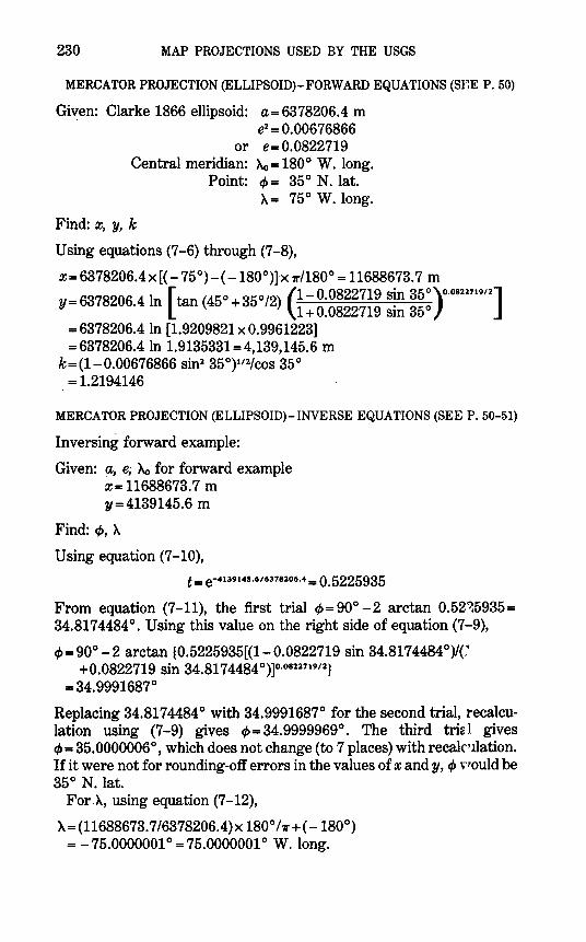
230 MAP PROJECTIONS USED BY THE USGS
MERCATOR PROJECTION (ELLIPSOID)-FORWARD EQUATIONS (SF:E P. 50)
Gi~en: Clarke 1866 ellipsoid: a= 6378206.4 m e'- = 0.00676866
or e= 0.0822719 Central meridian: Ac,= 180° W. long.
Find: x, y, k
Point: cp = 35 ° N. lat. >-.= 75° W. long.
Using equations (7 -6) through (7 -8),
X= 6378206.4x [( -75°)-( -180°)] x 1r/180° = 11688673.7 m y=6378206.4ln [tan (45o+ 35o12) (1-0.0822719 s~n 35°)o.o82U19''-]
1+0.0822719 Sin 35° = 6378206.4 In [1.9209821 x 0.9961223] = 6378206.4 In 1.9135331 = 4,139,145.6 m
k=(1-0.00676866 sin'- 35°)112/cos 35° = 1.2194146
MERCATOR PROJECTION (ELLIPSOID)-INVERSE EQUATIONS (SEEP. 50-51)
Inversing forward example:
Given: a, e; Ac, for forward example x= 11688673.7 m y=4139145.6 m
Find:¢,}..
Using equation (7-10),
t = e-4139145.6/6378206.4 = 0.5225935
From equation (7-11), the first trial ¢=90° -2 arctan 0.52?.5935= 34.8174484°. Using this value on the right side of equation (7-9),
¢=90° -2 arctan (0.5225935[(1-0.0822719 sin 34.8174484°)/C +0.0822719 sin 34.8174484 °)]0·0822719''-J
= 34.9991687°
Replacing 34.8174484 ° with 34.9991687° for the second trial, recalculation using (7 -9) gives cp = 34.9999969°. The third tria 1 gives ¢=35.0000006°, which does not change (to 7 places) with recaknlation. If it were not for rounding-off errors in the values of x and y, cp vrould be 35° N. lat.
For.}.., using equation (7-12),
>-.=(11688673. 7/6378206.4)x 180°/7r+( -180°) = -75.0000001° = 75.0000001° W. long.
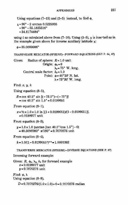
APPENDIXES
Using equations (7-13) and (3-5) instead, to find cp,
x = 90° -2 arctan 0.5225935 = 90°-55.1825516° = 34.817 4484 °
231
using t as calculated above from (7-10). Using (3-5), xis inse:--ted as in the example given above for inverse auxiliary latitude x:
cJ> = 35.0000006 °
TRANSVERSE MERCATOR (SPHERE)-FORWARD EQUATIONS (SEEP. 64, 67)
Given: Radius of sphere: R= 1.0 unit Origin: c/Jo = 0
Ao=75° W. long. Central scale factor: ko= 1.0
Point: c/J=40°30' N. lat. A= 73°30' W. long.
Find: x, y, k
Using equation (8-5),
B=cos 40.5° sin [(-73.5°)-(-75°)] =cos 40.5° sin 1.5° = 0.0199051
From equation (8-1),
x = 112 x 1.0 x 1.0 In [(1 + 0.0199051)/(1- 0.0199051)]. = 0.0199077 unit
From equation (8-3),
y= LOx 1.0 (arctan [tan 40.5°/cos 1.5°]-0} = 40.5096980° 1rll80° = 0. 7070276 unit
From equation (8-4),
k = 1.0/(1- 0.01990512}
112 = 1.0001982
TRANSVERSE MERCATOR (SPHERE)- INVERSE EQUATIONS (SEE P. 67)
Inversing forward example:
Given: R, c/Jo, Ao, ko for forward example X= 0.0199077 unit y = 0. 7070276 unit
Find: cp, A Using equation (8-8},
D = 0. 7070276/(1.0 x 1.0)+ 0 = 0. 7070276 radian
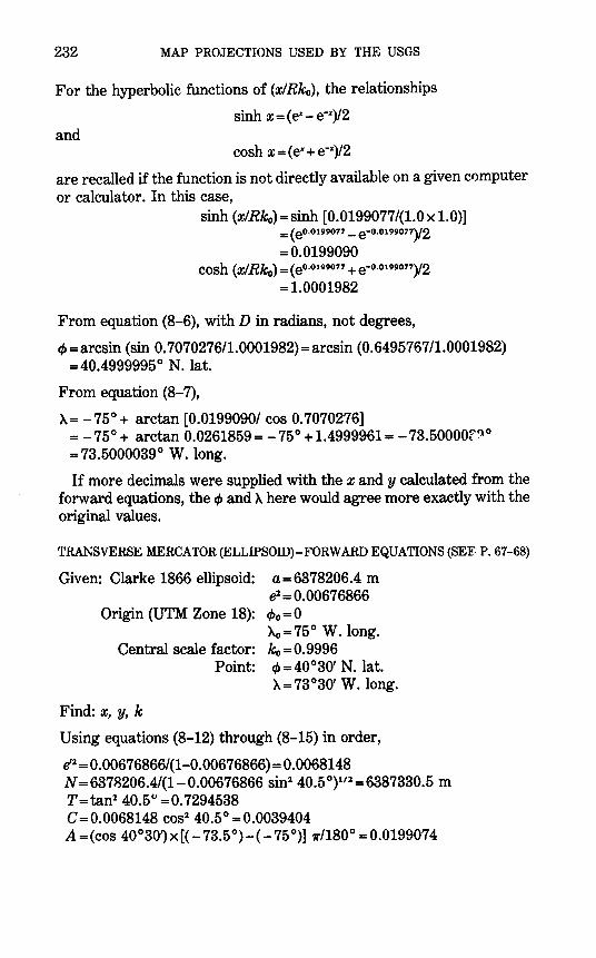
232 MAP PROJECTIONS USED BY THE USGS
For the hyperbolic functions of (x/Rko), the relationships
sinh x = (ex- e-")/2 and
cosh x = ( e" + e-")/2
are recalled if the function is not directly available on a given computer or calculator. In this case,
sinh (x/Rko) =sinh [0.0199077/(1.0 x 1.0)] = ( eo.o199o11 _ e-o.o199071)/2 =0.0199090
cosh (x/Rko) = ( eo.o199077 + e-o.o199077)/2 =1.0001982
From equation (8-6), with D in radians, not degrees,
cp =arcsin (sin 0. 7070276/1.0001982) =arcsin (0.6495767/1.0001982) =40.4999995° N. lat.
From equation (8-7),
A= -75° + arctan [0.0199090/ cos 0.7070276] = -75° + arctan 0.0261859 = -75° + 1.4999961 = -73.50000f~0
= 73.5000039° W. long.
If more decimals were supplied with the x and y calculated from the forward equations, the cf> and A here would agree more exactly with the original values.
TRANSVERSE MERCATOR (ELLIPSOID)- FORWARD EQUATIONS (SEF P. 67-68)
Given: Clarke 1866 ellipsoid: a= 6378206.4 m e1 = 0.00676866
Origin (UTM Zone 18): cf>o = 0 A0=75° W. long.
Central scale factor: ko=0.9996 Point: c/>=40°30' N. lat.
A=73°30' W. long.
Find: x, y, k
Using equations (8-12) through (8-15) in order,
e'1 = 0.00676866/(1-0.00676866) = 0.0068148 N = 6378206.4/(1- 0.00676866 sin1 40.5 °)111 = 6387330.5 m T = tan1 40.5 <~ = 0. 7294538 C=0.0068148 cos1 40.5° =0.0039404 A =(cos 40°30~x[( -73.5°)-( -75°)] 1rll80° =0.0199074
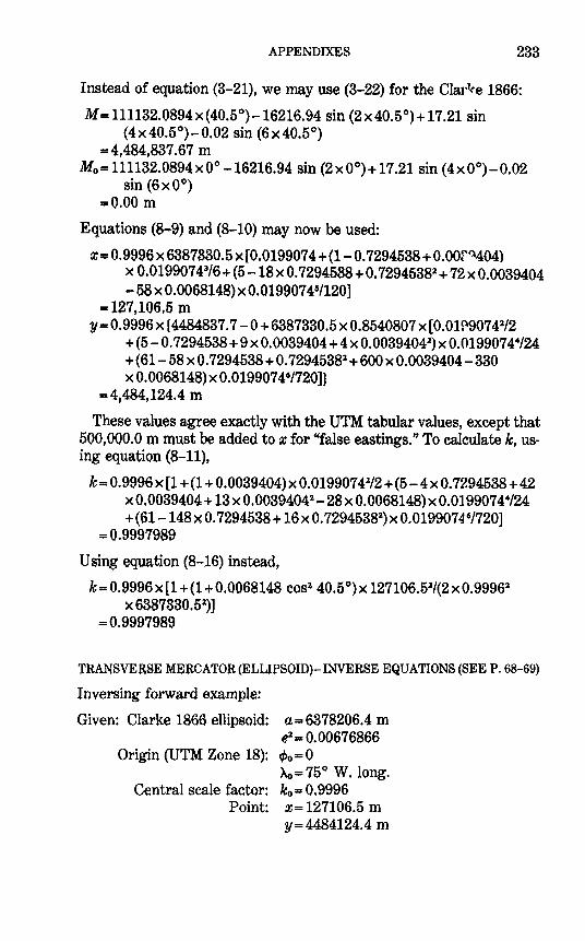
APPENDIXES 233
Instead of equation (3-21), we may use (3-22) for the Clar~e 1866:
M=111132.0894x(40.5°)-16216.94 sin (2x40.5°)+17.21 sin (4x40.5°)-0.02 sin (6x40.5°)
=4,484,837.67 m Mo= 111132.0894x0° -16216.94 sin (2x0°)+ 17.21 sin (4x0°)-0.02
sin (6x0°) •0.00 m
Equations (8-9) and (8-10) may now be used:
x = o.9996 x 6387830.5 x [0.019907 4 + (1- o. 7294538 + o.oor(\404) X 0.019907 43/6 + (5 -18 X 0. 7294538 + 0. 72945382 + 72 X 0.0039404 -58 X 0.0068148) X 0.019907 41/120]
= 127,106.5 m y= 0.9996 X (4484837. 7-0 + 6387330.5 X 0.8540807 X [0.01!\90742/2
+(5-0.7294538+9x0.0039404+4x0.00394042)x0.01990744/24 +(61- 58 X 0. 7294538 + 0. 72945382 + 600 X 0.0039404-330 X 0.0068148) X 0.019907 46/720]}
= 4,484,124.4 m
These values agree exactly with the UTM tabular values, except that 500,000.0 m must be added to x for ''false eastings." To calculate k, using equation (8-11),
k=0.9996x[l+(l+0.0039404)x0.01990742/2+(5-4x0.7294538+42 x0.0039404+13x0.00894042 -28x0.0068148)x0.01990744/24 +(61-148x0.7294538+ 16x 0. 72945382)x0.0199074 6/720]
=0.9997989
Using equation (8-16) instead,
k=0.9996x[l +(1 +0.0068148 cos2 40.5°)X 127106.52/(2x0.99962
X 6387330.52)]
=0.9997989
TRANSVERSE MERCATOR (ELLIPSOID)- INVERSE EQUATIONS (SEEP. 68-69)
lnversing forward example:
Given: Clarke 1866 ellipsoid: a= 6378206.4 m 62 =0.00676866
Origin (UTM Zone 18): cl>o = 0 Ao=75° W. long.
Central scale factor: ko= 0.9996 Point: X= 127106.5 m
y=4484124.4 m
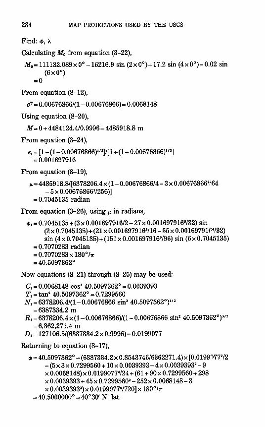
234 MAP PROJECTIONS USED BY THE USGS
Find: cp, A
Calculating Mo from equation (3-22),
M0 =111132.089x0°-16216.9 sin (2x0°)+17.2 sin (4x0°)-0.02 sin (6x0°)
=0
From equation (8-12),
lfl= 0.00676866/(1- 0.00676866)= 0.0068148
Using equation (8-20),
M=0+4484124.4/0.9996=4485918.8 m
From equation (3-24),
e1 = [1- (1- 0.00676866)112]/[1 + (1- 0.00676866)112]
= 0.001697916
From equation (8-19),
p.= 4485918.8/[6378206.4 X (1- 0.00676866/4-3 X 0.006768662/64 - 5 X 0.006768663/256)]
= 0. 7045135 radian
From equation (3-26), using p. in radians,
c/>1 = 0. 7045135 + (3 x 0.001697916/2- 27 x 0.0016979163/32) sin (2 X 0. 7045135)+ (21 X 0.0016979162/16-55 X 0.00169791(~4/32) sin (4x0.7045135)+(151x0.0016979163/96) sin (6x0.7045135)
= 0. 7070283 radian = 0. 7070283 x 180° 17r = 40.5097362°
Now equations (8-21) through (8-25) may be used:
c1 = 0.0068148 COS2 40.5097362° = 0.0039393 T1 = tan2 40.5097362° = 0. 7299560 N1 = 6378206.4/(1- 0.00676866 sin2 40.5097362°)112
= 6387334.2 m R1 = 6378206.4 x (1- 0.00676866)/(1- 0.00676866 sin2 40.5097362°)312
= 6,362,271.4 m D1 = 127106.5/(6387334.2 X 0.9996) = 0.0199077
Returning to equation (8-17),
cp = 40.5097362°- (6387334.2 X 0.85437 46/6362271.4) X [0.01991772/2 - (5 X 3 X 0. 7299560 + 10 X 0.0039393-4 X 0.00393932
- 9 x0.0068148)x0.01990774/24+(61+90x0.7299560+298 X 0.0039393 + 45 X 0. 72995602 -252 X 0.0068148-3 x 0.00393932)x 0.01990776/720] x 180° /r
= 40.5000000° = 40°30' N. lat.
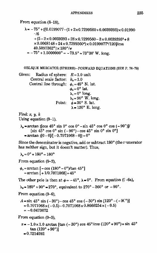
APPENDIXES
From equation (8-18),
A= -75° + {[0.0199077 -(1 + 2x0. 7299560+0.0039393)x 0.01990. -/6 +(5-2 X 0.0039393 + 28 X 0. 7299560-3 X 0.00393932 + 8 x 0.0068148 + 24 x 0. 72995602) x 0.01990775/120]/cos 40.5097362°} X 180° f1r
= -75° + 1.5000000° = -73.5° = 73°30' W. long.
235
OBLIQUE MERCATOR (SPHERE)- FORWARD EQUATIONS (SEEP. 76-78)
Given: Radius of sphere: R = 1.0 unit Central scale factor: k0 = 1.0
Central line through: c/> 1 = 45 ° N. lat. c/>2=0° lat.
Find: x, y, k
A1 =0° long. A2=90° W. long.
Point: c/> = 30° S. lat. A= 120° E. long.
Using equation (9-1),
Ap=arctan {[cos 45° sin 0° cos 0°-sin 45° cos 0° cos (-90")]/ [sin 45° cos 0° sin ( -90°)-cos 45° sin 0° sin 0°]
=arctan {[0-0]/[ -0.7071068-0]} =0°
Since the denominator is negative, add or subtract 180° (the r,1merator has neither sign, but it doesn't rnatter). Thus;
Ap = oo + 180° = 180°
From equation (9-2);
c/>,=arctan [-cos (180° -0°)/tan 45°] =arctan [ +1/0.7071068]=45°
The other pole is then at cf> = - 45 °, A= 0°. From equation (f-6a),
A.o = 180° + 90° = 270°, equivalent to 270°- 360° or -90°.
From equation (9-6),
A= sin 45 ° sin (- 30°)- cos 45 ° cos (- 30°) sin [120° - (- 9~ 0 )]
=0.7071068x( -0.5)-0.7071068x0.8660254x( -0.5) = -0.0473672
From equation (9-3),
X= -l.Oxl.O arctan [tan (-30°) cos 45°/cos (120°+90°)+sin 45° tan (120° + 90°)]
=0.7214592
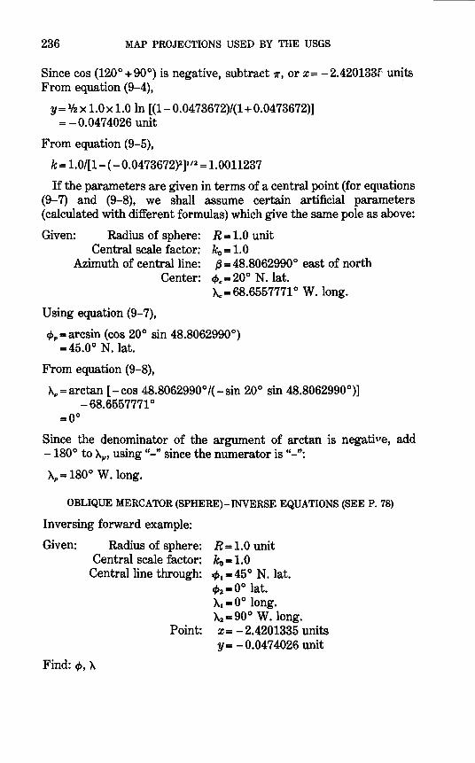
236 MAP PROJECTIONS USED BY THE USGS
Since cos (120° +90°) is negative, subtract 1r, or X= -2.420133f units From equation (9-4),
y= 1/2xl.Oxl.O ln [(1-0.0473672)/(1+0.0473672)] = -0.0474026 unit
From equation (9-5),
k= 1.0/[1- (- 0.0473672}1]112 = 1.0011237
If the parameters are given in terms of a central point (for eqnations (9-7) and (9-8), we shall assume certain artificial parameters (calculated with different formulas) which give the same pole as above:
Given: Radius of sphere: R = 1.0 unit Central scale factor: ko= 1.0
Azimuth of central line: {3 = 48.8062990° east of north Center: cl>c = 20° N. lat.
Ac:=68.6557771 ° W. long.
Using equation (9-7),
c/>p=arcsin (cos 20° sin 48.8062990°) =45.0° N. lat.
From equation (9-8),
~p =arctan [-cos 48.8062990° /(-sin 20° sin 48.8062990°)] - 68.6557771°
=00
Since the denominator of the argument of arctan is negative, add -180° to Ap., using "-" since the numerator is "-":
~p= 180° W.long.
OBLIQUE MERCATOR (SPHERE)- INVERSE EQUATIONS (SEE P. 78)
Inversing forward example:
Given: Radius of sphere: R= 1.0 unit Central scale factor: ko •1. 0
Central line through: '4> 1 = 45 ° N. lat. c/>2=0° lat. ~1=0° long. ~2=90° W.long.
Find: q,, ~
Point: X= -2.4201335 units y= -0.0474026 unit
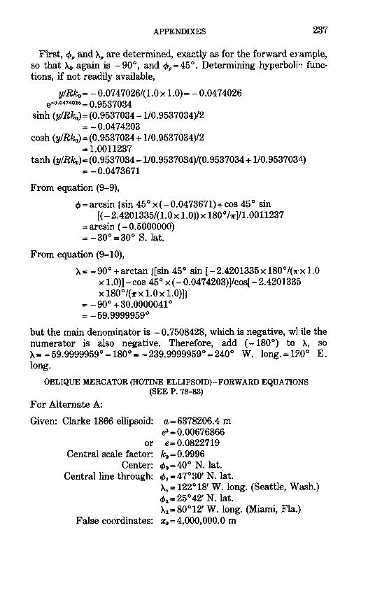
APPENDIXES 237
First, cpp and Ap are determined, exactly as for the forward e:rample, so that Ao again is - 90 °, and cpp = 45 °. Determining hyperboli ~ functions, if not readily available,
y!Rk0 = -0.0747026/(l.Ox 1.0)= -0.0474026 e-0 ·
0474026 = 0.9537034 sinh (y/Rk0)=(0.9537034-1/0.9537034)/2
= -0.0474203 cosh (y/Rk0)=(0.9537034+ 1/0.9537034)/2
= 1.0011237 tanh (y/Rk0)=(0.9537034-1/0.9537034)/(0.9537034+ 1/0.953703-1)
= -0.0473671
From equation (9-9),
<j}=arcsin {sin 45°x(-0.047g671)+cos 45° sin [(- 2.4201gg5f(1.0 X 1.0)) X 180° f1r]/1.00112g7
=arcsin (- 0.5000000) = -goo= goo S. lat.
From equation (9-10),
A= -90° +arctan {[sin 45° sin [ -2.4201gg5x 180°/(rx 1.0 x 1.0)]- cos 45 ° x (- 0.04 7 420g)]/cos[- 2.4201gg5 X 180°/(7rX l.Ox 1.0)]}
= -90° +g0.0000041 ° = -59.9999959°
but the main denominator is - 0. 7508428, which is negative, wNle the numerator is also negative. Therefore, add (- 180°) to A, so A=-59.9999959°-180°=-2g9.9999959°=240° W. long.=120° E. long.
OBLIQUE MERCATOR (HOTINE ELLIPSOID)-FORWARD EQUATIONS (SEE P. 78-83)
For Alternate A:
Given: Clarke 1866 ellipsoid: a= 6g78206.4 m e2 =0.00676866
or e=0.0822719 Central scale factor: k0 =0.9996
Center: <j}0 =40° N. lat. Central line through: cp1 =47°30' N. lat.
A1 = 122°18' W. long. (Seattle, Wash.) <j}1 =25°42' N. lat. A2 = 80°12' W. long. (Miami, Fla.)
False coordinates: x0 = 4,000,000.0 m
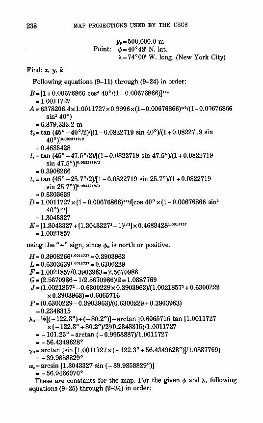
238 MAP PROJECTIONS USED BY THE USGS
Find: x, y, k
Yo=500,000.0 m Point: c/)=40°48' N. lat.
A=74°00' W. long. (New York City)
Following equations (9-11) through (9-24) in order:
B = [1 + 0.00676866 cos4 40° /(1- 0.00676866)]1/l = 1.0011727
A=6378206.4xl.0011727x0.9996x(1-0.00676866)112/(1-0.Qi1676866 sin2 40°)
= 6,379,333.2 m t0 =tan (45° -40°/2)/[(1-0.0822719 sin 40°)/(1+0.0822719 sin
400)]0.0822719/l
=0.4683428 t1 =tan (45°- 47.5° /2)/[(1- 0.0822719 sin 47.5°)/(1 + 0.0822719
sin 4 7.5 o)]o.o822719/2 =0.3908266
t2 =tan (45°- 25.7° /2)/[1- 0.0822719 sin 25. 7°)/(1 + 0.0822719 sin 25. 7o)]o.o822719/2
=0.6303639 D = 1.0011727 x (1- 0.00676866)112/[ cos 40° x (1- 0.00676866 sin2
400)112] = 1.3043327
E = [1.3043327 + (1.30433272-1)112] X 0.4683428l.001l727
=1.0021857
using the "+" sign, since cPo is north or positive.
H = 0.39082661.0011127 = 0.3903963 L = 0.63036391.0011727 = 0.6300229 F= 1.0021857/0.3903963=2.5670986 G=(2.5670986-1/2.5670986)/2= 1.0887769 J = (1.00218572- 0.6300229 X 0.3903963)/(1.00218572 + 0.6300229
X 0.3903963)= 0.6065716 p = (0.6300229- 0.3903963)/(0.6300229 + 0.3903963)
=0.2348315 Ac,=l/2((-122.3°)+(-80.2°)]-arctan (0.6065716 tan [1.0011727
X ( -122.3° + 80.2°)/2]/0.2348315)/1.0011727 = -101.25°- arctan (- 0.9953887)/1.0011727 = - 56.4349628 °
-y0 = ~ctan {sin [1.0011727 x ( -122.3° + 56.4349628°)]/1.0887769} = -39.9858829°
a.,= arcsin [1.30~3327 sin (- 39.9858829°)] = -56.9466070° These are constants for the map. For the given cP and A, following
equations (9-25) through (9-34) in order:
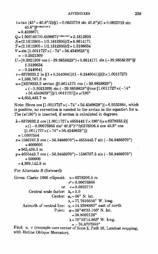
APPENDIXES
t= tan ( 45°-40.8° /2)/[(1- 0.0822719 sin 40.8°)/(1 + 0.0822719 sin 40.80)]0.0822719/2
=0.4598671 Q= 1.0021857/0.4598671LOOlt7l7 = 2.1812805 s = (2.1812805 -1/2.1812805)/2 = 0.8614171 T = (2.1812805 + 1/2.1812805)/2 = 1.3198634 V =sin [1.0011727 x ( -74 ° + 56.4349628°)]
= - 0.3021309
239
U = [0.3021309 cos (- 39.9858829°)+ 0.8614171 sin (- 39.~858~29°)]/ 1.3198634
= - 0.2440041 V= 6379333.2 In [(1 + 0.2440041)/(1- 0.2440041)]/(2 x 1.0011727)
= 1,586,767.3 m U= [[6379333.2 arctan ([0.8614171 cos (- 39.9858829°)
+ (- 0.3021309) sin (- 39.9858829°)]/cos [1.0011727 x ( -7 4 ° + 56.4349628°)]}/1.0011727]] X 71"/180°
= 4,655,443. 7 m
Note: Since cos [1.0011727x( -74° +56.4349628°)]=0.9532664, which is positive, no correction is needed to the arctan in the equatio~ for u. The (11"/180°) is inserted, if arctan is calculated in degrees.
k= 6379333.2 cos [1.0011727x4655443.7x 180°/(7rX 6379333.2)] x (1- 0.00676866 sin2 40.8°)l12/(6378206.4 cos 40.8° cos [1.0011727 X ( -74 ° + 56.4349628°)]}
= 1.0307554 x= 1586767.3 cos (- 56.9466070°) + 4655443.7 sin (- 56.9466070°)
+4000000 = 963,436.1 m
y=4655443.7 cos (- 56.9466070°)-1586767.3 sin (- 56.9466070°) +500000
= 4,369,142.8 m
For Alternate B (forward):
Given: Clarke 1866 ellipsoid: a= 6378206.4 m e2 = 0.00676866
or e= 0.0822719 Central scale factor: ko = 1.0
Center: c/>0 = 36 ° N. lat. Ac=77.7610558° W. long.
Azimuth of central line: ac= 14.3394883° east of north Point: c/>=38°48'33.166" N. lat.
= 38.8092128° A= 76°52'14.863" W. long.
. = -76.870795R 0
Fmd: u, v (example uses center of Zone 2, Path 16, Landsat mapping, with Hotine Oblique Mercator).
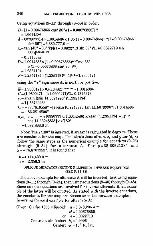
240 MAP PROJECTIONS USED BY THE USGS
U;:;ing equations (9-11) through (9-39) in order,
B = [1 + 0.00676866 cos4 36° /(1- 0.00676866)]1H
=t0014586 A= 63780206.4 X 1.0014586 X 1.0 X (1- 0.00676866}112/(1- 0.00~76866
sin2 36°)= 6,380, 777,0 m t0=tan (45° -36°/2)/[(1-0.0822719 sin 36°)/(1+0.0822719 sin
360)]0.0812719/2 =0.5115582
D = 1.0014586 x (1- 0.00676866}112/[cos 36° x (1- 0.00676866 sin2 36°)1'2]
= 1.2351194 F= 1.2351194+(1.2351194~ -1}112 = 1.9600471
using the "+ " sign since cp0 is north or positive.
E = 1.9600471 X 0,51155821.0014586 = 1.0016984 G=(l.9600471--1/1.9600471)/2= 0. 7249276 'Yo= arcsin [(sin 14.3394883°)/1.2351194]
= 11.5673996° Ap= ~ 77.7610558°- [arcsin (0. 7249276 tan 11.5673996Q)]/1.0114586
= -86.2814800° U<36o, _ 77.76 ... a)=+ (6380777.0/1,0014586) arctan [(1.23511942-1)1n/
COS 14.3394883°] X 11'/180° =4,092,868.9 m -
Note: The 11"1180° is inserted, if arctan is calculated in degrf~S. These are constants for the map. The calculations of u, v, x, andy for (q,, >..) follow the same steps as the numerical example for equaticns (9-25) through (9-34) for alternate A. For (/) = 38.8092128° and >.. = -76.8707953 o, it is found tb~t
U= 4,414,439.0 m v = - 2.356.3 m
OBLIQUE MERCATOR (HOTINE ELLIPSOID)- INVERSE EQUAT ... 4)NS (SEE P. 83-84)
The above example for alternate A will be inverted, first using equations (9-11) through (9-24}, then using equations (9-40) through (9-48). Since no new equations are involved for inverse alternate B, -an example of the latter will be omitted. As stated with the inverse e1uations, the constants for the map are chosen as in the forward exan1ples. Inversing forward example for alternate A:
Given: Clarke 1866 ellipsoid: a= 6,378,206.4 m e2 = 0.00676866
or e= 0.0822719 Central scale factor: ko = 0.9996
Center: c/>0 = 40° N. lat.
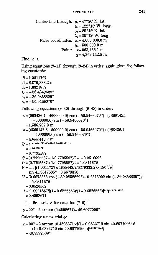
APPENDIXES
Center line through: cf>1 = 4 7° 30' N. lat.
Find: q,, A
A1 = 1~2°18' W. long. cP2 = 25°42' N. lat. A2=80°12' W. long.
False coordinates: X0 =4,000,000.0 m Yo= 500,000.0 m
Point: x = 963,436.1 m y=4,369,142.8 m
241
Using equations (9-11) through (9-24) in order, again gives the following constants:
B=1.0011727 A= 6,379,333.2 m E = 1.0021857 Ao = - 56.4349628° 'Yo= -39.9858829° O:c = - 56.9466070°
Following equations (9-40) through (9-48) in order:
v=(963436.1-40ooooo.o) cos ( -56.9466070°)-(4369142.r - 500000.0) sin (- 56.9466070°)
= 1,586, 767.3 m U=(4369142.8- 500000.0) COS ( -56.9466070°)+(963436.1
- 4000000.0) sin (- 56.9466070°) = 4,655,443. 7 m
Q' = e-C1.0011727x1586767.3/6379333.2) = e-0.2490273
=0.7795587 S' = (0. 7795587-110. 7795587)/2 = - 0.2516092 T' = (0. 7795587 + 1/0. 7795587)/2 = 1.0311679 V =sin [(1.0011727x 4655443. 7/6379333.2)x 180°/r]
=sin 41.8617535° = 0.6673356 U' = [0.6673356 cos (- 39.9858829°)- 0.2516092 sin (- 39.9858829°)]/
1.0311679 =0.6526562
t= (1.0021857/[(1 + 0.6526562)/(1- 0.6526562)]112]111·0011727
=0.4598671
The first trial q, for equation (7-9) is
f/>=90° -2 arctan (0.4598671)=40.6077096°
Calculating a new trial q,:
<P = 90°-2 arctan {0.4598671 x [(1- 0.0822719 sin 40.6077096°)/ (1 + 0.0822719 sin 40.6077096°)]0·082271912)
= 40.7992509°
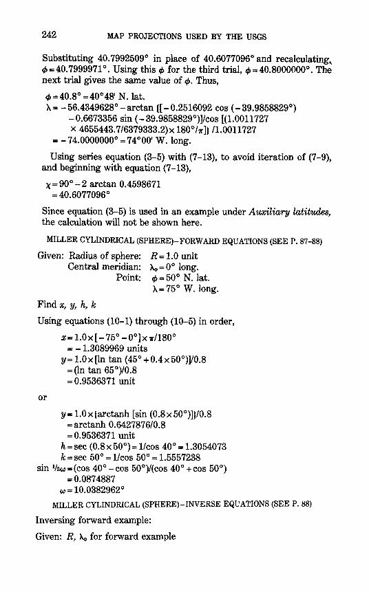
242 MAP PROJECTIONS USED BY THE USGS
Substituting 40.7992509° in place of 40.6077096° and recalculating,, q, = 40.7999971°. Using this q, for the third trial, q, = 40.8000000°. The next trial gives the same value of q,. Thus,
4>=40.8° =40°48' N. lat. A= -56.4349628°- arctan {[- 0.2516092 cos (- 39.9858829°)
-0.6673356 sin (- 39.9858829°)]/cos [(1.0011727 x 4655443.7/6379333.2)x 180°/11"]} /1.0011727
= -74.0000000°=74°00' W. long.
Using series equation (3-5) with (7 -13), to avoid iteration of (7 -9), and beginning with equation (7 -13),
x = 90°-2 arctan 0.4598671 =40.6077096°
Since equation (3-5) is used in an example under Auxiliary latitudes, the calculation will not be shown here.
MILLER CYLINDRICAL (SPHERE)- FORWARD EQUATIONS (SEEP. 87-88)
Given: Radius of sphere: R= 1.0 unit Central meridian: Xo = 0° long.
Point: q, = 50° N. lat. A=75° W. long.
Find x, y, h, k
Using equations (10-1) through (10-5) in order,
X= 1.0 X [ -75°- 0°] X 11"/180°
or
= - 1.3089969 units y=l.Ox[ln tan (45°+0.4x50°)]/0.8
=(In tan 65°)/0.8 = 0.9536371 unit
y= 1.0 x {arctanh [sin (0.8x 50°)]}/0.8 =arctanh 0.6427876/0.8 = 0.9536371 unit
h= sec (0.8x 50°)= 1/cos 40° = 1.3054073 k =sec 50° = 1/cos 50° = 1.5557238
sin 112w =(cos 40°- cos 50°)/(cos 40° +cos 50°) =0.0874887
w= 10.0382962°
MILLER CYLINDRICAL (SPHERE)- INVERSE EQUATIONS (SEE P. 88)
Inversing forward example:
Given: R, Xo for forward example
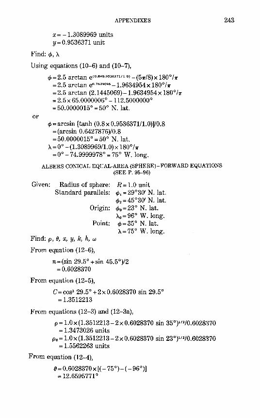
X= -1.3089969 units y= 0.9536371 unit
APPENDIXES
Find:¢,~
Using equations (10-6) and (10-7),
or
¢ = 2.5 arctan e< 0 · 8 ,.0 · 95363711 .. 0 >- (5?r/8) x 180° l1r = 2.5 arctan e0
·7629096 -1.9634954 x 180° l1r
= 2.5 arctan (2.1445069)-1.9634954x 180°/?r = 2.5 X 65.0000006°-112.5000000° = 50.0000015° = 50° N. lat.
¢=arcsin [tanh (0.8 x 0.9536371/1.0)]/0.8 =(arcsin 0.6427876)/0.8 = 50.0000015° = 50° N. lat.
~ = 0°- (1.3089969/1.0) X 180° /1r =0°-74.9999978°=75° W.long.
ALBERS CONICAL EQUAL-AREA (SPHERE)-FORWARD EQUATIONS (SEE P. 95-96)
Given: Radius of sphere: R = 1.0 unit Standard parallels: ¢ 1 =29°30' N. lat.
c/>2 = 45°30' N. lat. Origin: ¢0 = 23 ° N. lat.
~=96° W. long. Point: ¢=35° N. lat.
~=75° W. long. Find: p, 0, x, y, k, h, w
From equation (12-6),
n= (sin 29.5° +sin 45.5°)/2 =0.6028370
From equation (12-5),
C=cos2 29.5° +2x0.6028370 sin 29.5° = 1.3512213
From equations (12-3) and (12-3a),
p = 1.0 x (1.3512213- 2 x 0.6028370 sin 35°)112/0.6028370 = 1.3473026 units
Po= 1.0 x (1.3512213- 2 x 0.6028370 sin 23°)112/0.6028370 = 1.5562263 units
From equation (12-4),
0= 0.6028370 X (( -75°)- (- 96°)] = 12.6595771°
243
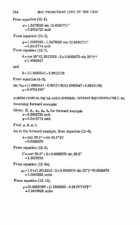
244 MAP PROJECTIONS USED BY THE USGS
From equation (12-1),
X= 1.3473026 sin 12.6595771° = 0.2952720 unit
From equation (12-2),
y= 1.5562263-1.3473026 cos 12.6595771 o
= 0.241677 4 unit From equation (12-7),
and
h=cos 35°/(1.3512213-2x0.6028370 sin 35°)112
= 1.0085547
k= 1/1.0085547 = 0.9915178
From equation ( 4-9),
sin 112w= 11.0085547- 0.9~151781/(1.0085547 +0.9915178) w=0.9761189°
ALBERS CONICAL EQUAL-AREA (SPHERE)- INVERSE EQUATIONS (f!~E P. 96)
Inversing forward example:
Given: R, ck_~~ c/>2, cf>o, Ao for forward example x = 0.2952720 unit y=0.2416774 unit
Find: p, 8, cp, A
As in the forward example, from equation (12-6),
n= (sin 29.5° +sin 45.5°)/2 =0.6028370
From equation (12-5),
C=cos2 29.5° +2x0.6028370 sin 29.5° = 1.3512213
From equation (12-3a),
po= l.Ox(l.3512213-2x0.6028370 sin 23°)112/0.6028370 = 1.5562263 units
From equation (12-10),
p = [0.29527202 + (1.5562263- 0.241677 4)2]
112
= 1.3473026 units
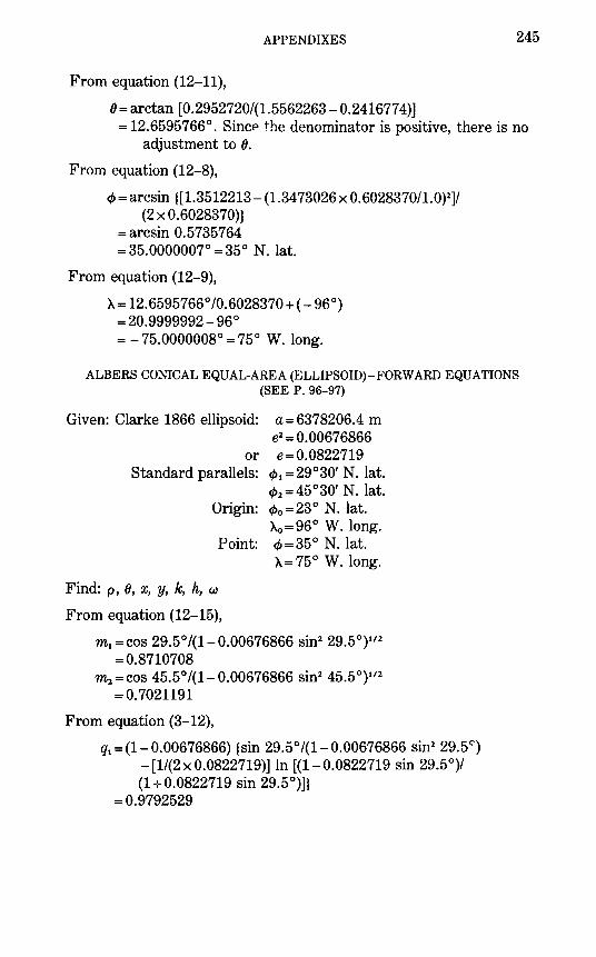
APPENDIXES 245
From equation (12-11),
8 =arctan [0.2952720/(1.5562263- 0.241677 4)] = 12.6595766°. SincP the denominator is positive, there is no
adjustment to 8.
From equation (12-8),
cJ> =arcsin {[1.3512213- (1.34 73026 x 0.6028370/1.0)2]/
(2 X 0.6028370)} =arcsin 0.5735764 =35.0000007°=35° N. lat.
From equation (12-9),
>..= 12.6595766°/0.6028370 + (- 96°) = 20.9999992- 96 ° = -75.0000008° = 75° W. long.
ALBERS CONICAL EQUAL-AREA (ELLIPSOID)- FORWARD EQUATIONS (SEE P. 96-97)
Given: Clarke 1866 ellipsoid: a= 6378206.4 m e2 = 0.00676866
or e=0.0822719 Standard parallels: ¢ 1 =29°30' N. lat.
¢ 2 =45°30' N. lat. Origin: ¢ 0 = 23 ° N. lat.
>..o=96° W. long. Point: cJ> = 35 o N. lat.
>..=75° W. long.
Find: p,8, ~ ~ ~ ~ w
From equation (12-15),
m1 =cos 29.5° /(1- 0.00676866 sin2 29.5°)112
=0.8710708 m2 =cos 45.5° /(1- 0.00676866 sin2 45.5°)112
=0.7021191
From equation (3-12),
q1 =(1-0.00676866) {sin 29.5°/(1-0.00676866 sin2 29.5c) - [1/(2 x 0.0822719)] ln [(1- 0.0822719 sin 29.5°)/ (1 + 0.0822719 sin 29.5°)]}
=0.9792529
246 MAP PROJECTIONS USED BY THE USGS
Using the same formula for q2 (with ¢2 instead of ¢ 1),
q2 = 1.4201080
Using the same formula for q0 (with ¢0 instead of ¢ 1),
q0 = 0. 7767080
From equation (12-14),
n= (0.87107082- 0. 70211912)/(1.4201080- 0.9792529)
=0.6029035
From equation (12-13),
C = 0.87107082 + 0.6029035 X 0.9792529 = 1.3491594
From equation (12-12a),
p0 = 6378206.4 X (1.3491594- 0.6029035 X 0. 7767080)112/0.6029035 =9,929,079.6 m
These are the constants for the map. For ¢=35° N. lat. and A=75° W. long.: Using equation (3-12), but with¢ in place of¢.,
q= 1.1410831
From equation (12-12),
p = 6378206.4 X (1.3491594- 0.6029035 X 1.1410831)112/0.6029035 = 8,602,328.2 m
From equation (12-4),
8 = 0.6029035 X ( -75°- (- 96°)] = 12.6609735°
From equation (12-1),
X=8602328.2 sin 12.6609735° = 1,885,472.7 m
From equation (12-2),
y= 9929079.6-8602328.2 cos 12.6609735° = 1,535,925.0 m
From equation (12-15),
m =cos 35 ° /(1- 0. 00676866 sin2 35 °)112
=0.8200656
From equation (12-16),
k = 8602328.2 X 0.6029035/(6378206.4 X 0.8200656) =0.9915546
From equation (12-18),
h= 110.9915546= 1.0085173
From equation ( 4-9),
APPENDIXES
sin 1/zw= 11.0085173- 0.99155461/(1.0085173 + 0.9915546) w= 0.9718678°
247
ALBERS CONICAL EQUAL-AREA (ELLIPSOID)- INVERSE EQUATIONS (SEE P. 97 -98)
Inversing forward example:
Given: Clarke 1866 ellipsoid: a= 6378206.4 m e2 = 0.00676866
or e= 0.0822719 Standard parallel: ¢ 1 = 29°30' N. lat.
<1>2 = 45°30' N. lat.
Find: p, 0, ¢, A
Origin: <Po= 23 ° N. lat. Ao=96° W. long.
Point: X= 1,885,472.7 m y= 1,535,925.0 m
The same constants n, C, p0 are calculated with the same equations as those used for the forward example. For the particular point:
From equation (12-10),
p = [18854 72.72 + (9929079.6 -1535925.0)2]
112
= 8,602,328.3 m
From equation (12-11),
()=arctan [18854 72.7 /(9929079.6- 1535925.0)] =arctan 0.2246441 = 12.6609733°. The denominator is positive; therefore() if not
adjusted. From equation (12-19), q= [1.3491594- (8602328.3 X 0.6029035/6378206.4)2]/0.6029035
= 1.1410831
Using for the first trial <t> the arcsin of (1.141083112), or 34.7879983°, calculate a new <t> from equation (12-19),
<t>= 34.7879983° + [(1- 0.00676866 sin2 34. 7879983°)2/(2 cos 34.7879983°)] x {1.1410831/(1- 0.00676866)- sin 34.7879983° I (1-0.00676866 sin2 34.7879983°)+[1/(2x0.0822719)] In [(1- 0.0822719 sin 34. 7879983°)/(1 + 0.0822719 sin 34. 7879983°)]} X 180° f1r
= 34.9997335 °
248 MAP PROJECTIONS USED BY THE USGS
Note that 180°/r is included to convert to degrees. Replacing 34.7879983° by 34.9997335° for the second trial, the calculation using equation (12-19) now provides a third cJ> of 35.0000015°. A ro.calculation with this value results in no change to seven decimal places. (This does not give exactly 35° due to rounding-off errors in x andy.) Thus,
c/>=35.0000015° N. lat.
For the longitude use equation (12-9),
X=( -96°)+ 12.6609733°/0.6029035 = -75.0000003° or 75.0000003° W. long.
For scale factors, we revert to the forward example, since cJ> r.nd X are now known.
Series equation (3-18) may be used to avoid the iteration alY)Ve. Beginning with equation (12-21),
{3 =arcsin [1.1410831/(1- [(1- 0.00676866)/(2 x 0.0822719)] In [(1- 0.0822719)/(1 + 0.0822719)]}]
= 34.8781793°
An example is not shown for equation (3-18), since it is similar to the example for (3-5).
LAMBERT CONFORMAL CONIC (SPHERE)-FORWARD EQUATI0NS (SEEP. 105)
Given: ·Radius of sphere: R = 1.0 unit Standard parallels: c/>1 = 33° N. lat.
c/>2 = 45° N. lat. Origin: c/>0 = 23 ° N. lat.
Ao=96° W. long. Point: cJ> = 35 o N. lat.
Find: p, (), x, y, k
From equation (13-3),
X= 75° W. long.
n=ln (cos 33°/cos 45°)/ln [tan (45° +45°/2)/tan (45° +33°/2)] =0.6304777
From equation (13-2),
F=[cos 33° tan°·6304777 (45° +33°/2)]/0.6304777 = 1. 9550002 units
From equation (13-1a),
Po= 1. 0 x 1. 9550002/tan°·6304777 ( 45 ° + 23 ° /2)
= 1.5071429 units
APPENDIXES 249
The above constants apply to the map generally. For the specific cp and}.., using equation (13-1),
p = 1. 0 x 1. 9550002/tan°·6304777 ( 45 o + 35 o /2)
= 1.2953636 units
From equation (12-4),
0=0.6304777x[( -75°)-( -96°)] = 13.2400316°
From equations (12-1) and (12-2),
X= 1.29531336 sin 13.2400316° = 0.2966785 unit
Y= 1.5071429-1.2953636 cos 13.2400316° = 0.2462112 unit
From equation (13-4),
k =cos 33 o tan°·6304777 ( 45 o + 33 ° /2)/[ cos 35 ° tan°·6304777 ( 45 o
+ 35°/2)] =0.9970040
or from equation ( 4-5),
k=0.6304777x 1.2953636/(1.0 cos 35°) =0.9970040
LAMBERT CONFORMAL CONIC (SPHERE)-INVERSE EQUATIONS (SEE P. 105, 107)
Inversing forward example:
Given: R, cp11 cp2 , c/Jo, >..a for forward example x = 0.2966785 unit Y= 0.2462112 unit
Find: p, 0, cp, }..
After calculating n, F, and p0 as in the forward example, obtaining the same values, equation (12-10) is used:
p = [0.29667852 + (1.5071429- 0.2462112)2)lll
= 1.2953636 units
From equation (12-11),
0 =arctan [0.2966785/(1.5071429- 0.2462112)] = 13.2400329°. Since the denominator is positive, 0 is not
adjusted.
From equation (12-9),
>..= 13.2400329°/0.6304777 +(- 96°) = -74.9999981°=74.9999981° W.long.
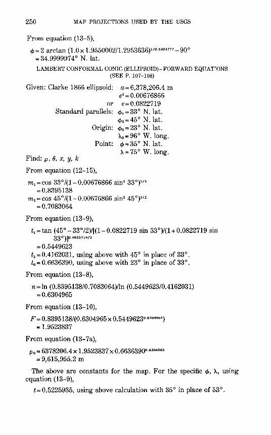
250 MAP PROJECTIONS USED BY THE USGS
From equation (13-5),
¢ = 2 arctan (1.0 x 1.9550002/1.2953636)110·6304777 - 90° = 34.9999974 o N. lat.
LAMBERT CONFORMAL CONIC (ELLIPSOID)- FORWARD EQUAT~ONS (SEE P. 107-108)
Given: Clarke 1866 ellipsoid: a= 6,378,206.4 m e2 = 0.00676866
or e=0.0822719 Standard parallels: ¢1 =33° N. lat.
¢2=45° N. lat. Origin: ¢0=23° N. lat.
A.o= 96° W. long. Point: ¢ = 35 o N. lat.
Find: p, 0, x, y, k A= 75° W. long.
From equation (12-15),
m1 =cos 33° /(1- 0.00676866 sin2 33°)112
=0.8395138 m2 =cos 45° /(1- 0.00676866 sin2 45°)112
=0.7083064
From equation (13-9),
t1=tan (45°-33°/2)/[(1-0.0822719 sin 33°)/(1+0.0822719 sin 330)]0.0822719/2
=0.5449623 t2 = 0.4162031, using above with 45° in place of 33°. t0 = 0.6636390, using above with 23° in place of 33°.
From equation (13-8),
n= ln (0.8395138/0. 7083064)/ln (0.5449623/0.4162031) =0.6304965
From equation (13-10),
F = 0.8395138/(0.6304965 X 0.5449623°·6304965) = 1.9523837
From equation (13-7a),
Po= 6378206.4x 1.9523837x 0.6636390°·6304965
= 9,615,955.2 m
The above are constants for the map. For the specific ¢, A, using equation (13-9),
t= 0.5225935, using above calculation with 35° in place of 33°.
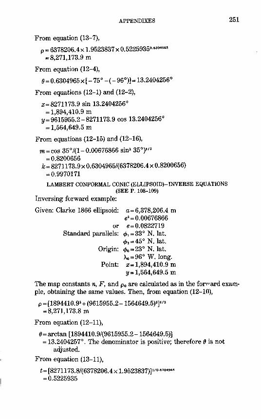
APPENDIXES
From equation (13-7),
p = 6378206.4 X 1.9523837 X 0.5225935°·6304965
=8,271,173.9 m
From equation (12-4),
8=0.6304965x[ -75° -( -96°)]= 13.2404256°
From equations (12-1) and (12-2),
X= 8271173.9 sin 13.2404256° = 1,894,410.9 m
y = 9615955.2-8271173.9 cos 13.2404256° = 1,564,649.5 m
From equations (12-15) and (12-16),
m=cos 35°/(1-0.00676866 sin2 35°)112
=0.8200656 k = 8271173.9 X 0.6304965/(6378206.4 X 0.8200656)
=0.9970171
LAMBERT CONFORMAL CONIC (ELLIPSOID)-INVERSE EQUATIONS (SEE P. 108-109)
Inversing forward example:
Given: Clarke 1866 ellipsoid: a= 6,378,206.4 m e2=0.00676866
or e= 0.0822719 Standard parallels: l/>1 =33° N. lat.
l/>2=45o N. lat. Origin: l/>0 = 23 ° N. lat.
Ao=96° W. long. Point: X= 1,894,410.9 m
y=1,564,649.5 m
251
The map constants n, F, and p0 are calculated as in the for,vard example, obtaining the same values. Then, from equation (12-10),
p = [1894410.92 + (9615955.2 -1564649.5)2]112
= 8,271,173.8 m
From equation (12-11),
8 =arctan [1894410.9/(9615955.2 -1564649.5)] = 13.2404257°. The denominator is positive; therefore 8 is not
adjusted.
From equation (13-11),
t= (8271173.8/(6378206.4 X 1.9523837)]1'
0·63
04965
=0.5225935
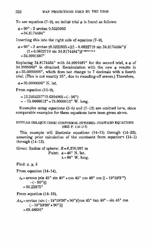
252 MAP PROJECTIONS USED BY THE USGS
To use equation (7-9), an initial trial cJ> is found as follows:
cJ> = 90°- 2 arctan 0.5225935 = 34.817 4484 °
Inserting this into the right side of equation (7 -9),
c/>=90° -2 arctan (0.5225935x[(l-0.0822719 sin 34.8174484°)/ (1 + 0.0822719 sin 34.8174484 °)]0 ·0822719/1
= 34.9991687°
Replacing 34.8174484 o with 34.9991687° for the second trial, a cJ> of 34.9999969° is obtained. Recalculation with the new c/J results in c/J = 35.0000006°, which does not change to 7 decimals with a fourth trial. (This is not exactly 35 °, due to rounding-off errors.) Therefore,
c/J=35.0000006° N. lat.
From equation (12-9),
= 13.2404257°/0.6304965+( -96°) = -75.0000013° = 75.0000013° W. long.
Examples using equations (3-5) and (7 -13) are omitted he"""e, since comparable examples for these equations have been given above.
BIPOLAR OBLIQUE CONIC CONFORMAL (SPHERE)-FORWARD EQUATIONS (SEEP. 114-117)
This example will illustrate equations (14-11) through (14-23), assuming prior calculation of the constants from equatior\3 (14-1) through (14-13).
Given: Radius of sphere: R = 6,370,997 m Point: c/J=40° N. lat.
A=90° W. long.
Find: x, y, k
From equation (14-14),
Zs= arccos (sin 45° sin 40° +cos 45° cos 40° cos [( -19°59'3~'~ -( -90°)]}
=50.22875°
From equation (14-15),
A Zs = arctan (sin (- 19 ° 59'36" + 90 ° )/[cos 45 ° tan 40 ° - sin 45 ° cos ( -19° 59'36'' + 90°)]}
=69.48856°
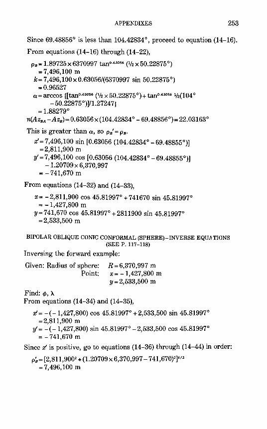
APPENDIXES 253
Since 69.48856° is less than 104.42834°, proceed to equation (14-16).
From equations (14-16) through (14-22),
p8 = 1.89725 x 6370997 tan°· 63056 (112 x 50.22875 °) = 7,496,100 m
k= 7,496,100 x 0.63056/(6370997 sin 50.22875°) =0.96527
a= arccos {[tan°·63056 (112 x 50.22875 °) + tan°· 63056 112(104 o
- 50.22875°)]/1.2724 7) = 1.88279°
n(AzsA -Az8 )= 0.63056x (104.42834 °- 69.48856°)= 22.03163°
This is greater than a, so ps' = Ps·
x = 7,496,100 sin [0.63056 (104.42834 o- 69.48855°)] = 2,811,900 m
y' = 7,496,100 cos [0.63056 (104.42834 °- 69.48855°)] -1.20709 X 6,370,997
= -741,670 m
From equations (14-32) and (14-33),
X= -2,811,900 cos 45.81997° +741670 sin 45.81997° = -1,427,800 m
y=741,670 cos 45.81997° +2811900 sin 45.81997° =2,533,500 m
BIPOLAR OBLIQUE CONIC CONFORMAL (SPHERE)-INVERSE EQUATIONS (SEE P. 117-118)
Inversing the forward example:
Given: Radius of sphere: R = 6,370,997 m
Find:¢, A.
Point: X= -1,427,800 m y = 2,533,500 m
From equations (14-34) and (14-35),
x = - (- 1,427,800) cos 45.81997° + 2,533,500 sin 45.81997° = 2,811,900 m
y' = - (- 1,427,800) sin 45.81997°-2,533,500 cos 45.81997° = -741,670 m
Since xis positive, go to equations (14-36) through (14-44) in order:
p~ = [2,811,9002 + (1.20709 X 6,370,997-7 41,670)2]
112
= 7,496,100 m
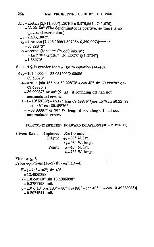
254 MAP PROJECTIONS USED BY THE USGS
A~=arctan [2,811,900/(1.20709x 6,370,997 -741,670)] = 22.03150° (The denominator is positive, so there is no
quadrant correction.) Ps=7,496,100 m Zs= 2 arctan [7,496,100/(1.89725x 6,370,997)]110·63056
=50.22873° a= arccos {[tan°·63056
( 1/2 x 50.22873°) + tan°·63056 112(104 °- 50.22873°)]/ 1.2724 7}
= 1.88279°
Since Az~ is greater than a, go to equation (14-42).
Azs= 104.42834°-22.03150°/0.63056 =69.48876°
cJ>=arcsin (sin 45° cos 50.22873° +cos 45° sin 50.22873° c1s 69.48876°)
= 39.99987° or 40° N. lat., if rounding off had not accumulated errors.
A= ( -19° 59'36")- arctan {sin 69.48876° /[cos 45 o /tan 50.22-:-~73° -sin 45° cos 69.48876°]}
= -89.99987° or 90° W. long., if rounding off had not accumulated errors.
POLYCONIC (SPHERE)-FORWARD EQUATIONS (SEEP. 128-129)
Given: Radius of sphere: Origin:
Point:
Find: x, y, h
R=l.O unit c/>0 =30° N. lat. Ao=96° W. long. cJ>=40° N. lat. A=75° W. long.
From equations (15-2) through (15-4),
E = (- 75 ° + 96 o) sin 40° = 13.4985398 °
x= 1.0 cot 40° sin 13.4985398° = 0.2781798 unit
y = 1.0 x [ 40° x 11'/180°- 30° x 11'1180° +cot 40° (1- cos 13.49~5398°)] = 0.207 4541 unit
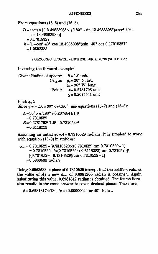
APPENDIXES
From equations (15-6) and (15-5),
D =arctan [(13.4985398° x r/180°- sin 13.4985398°)/(sec2 40°cos 13.4985398°)]
= 0.17018327° h = (1- cos2 40° cos 13.4985398°)/sin2 40° cos 0.17018327-:~
= 1.0392385
POLYCONIC (SPHERE)- INVERSE EQUATIONS (SEE P. 12~~
Inversing the forward example:
Given: Radius of sphere: R= 1.0 unit Origin: q,0 =30° N. lat.
~=96° W.long.
Find: q,, A
Point: x= 0.2781798 unit y=0.2074541 unit
Since y ::1: -1.0 X 30° X r/180°, use equations (15-7) and (15-8):
A= 30° X r/180° + 0.2074541/1.0 =0.7310529
B = 0.27817982/1.02 + 0. 73105292
=0.6118223
255
Assuming an initial q," =A= 0. 7310529 radians, it is simplest to work with equation (15-9) in radians:
q,n+t = 0. 7310529- (0. 7310529 X (0. 7310529 tan 0. 7310529 + 1) - 0.7310529- 1/2(0.73105292 +0.6118223) tan 0.731052~]/ [(0. 7310529-0. 7310529)/tan 0. 7310529 -1]
= 0.6963533 radian
Using 0. 6963533 in place of 0. 7310529 (except that the boldfar~ retains the value of A) a new q,n+t of 0.6981266 radian is obtainei. Again substituting this value, 0.6981317 radian is obtained. The fourth iteration results in the same answer to seven decimal places. Therefore,
q,=0.6981317x180°IT=40.0000004° or 40° N. lat.
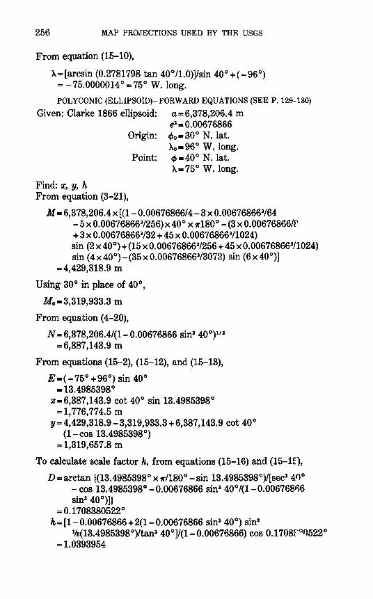
256 MAP PROJECTIONS USED BY THE USGS
From equation (15-10),
A=[arcsin (0.2781798 tan 40°/1.0)]/sin 40° +( -96°) = -75.0000014° =75° W. long.
POLYCONIC (ELLIPSOID)-FORWARD EQUATIONS (SEEP. 129-130)
Given: Clarke 1866 ellipsoid: a= 6,378,206.4 m e2 = 0.00676866
Origin: t/>0 =30° N. lat. Ao=96° W. long.
Point: t/>=40° N. lat. A=75° W. long.
Find: x, y, h From equation (3-21),
M = 6,378,206.4 X [(1- 0.00676866/4-3 X 0.006768662/64 - 5 X 0.006768663/256) X 40° X 1r 180°- (3 X 0.00676866/r + 3 X 0.006768662/32 + 45 X 0.006768663/1024) sin (2 X 40°) + (15 X 0.006768662/256 + 45 X 0.006768663/1024) sin (4x40°)-(35x0.006768663/3072) sin (6x40°)]
= 4,429,318.9 m
Using 30 o in place of 40 o,
Mo=3,319,933.3 m
From equation ( 4-20),
N = 6,378,206.4/(1- 0.00676866 sin2 40°)112
=6,387,143.9 ttl
From equations (15-2), (15-12), and (15-13),
E=( -75° +96°) sin 40° = 13.4985398°
x=6,387,143.9 cot 40° sin 13.4985398° = 1, 776,77 4.5 m
y=4,429,318.9-3,319,933.3+6,387,143.9 cot 40° (1- cos 13.4985398 °)
= 1,319,657.8 m
To calculate scale factor h, from equations (15-16) and (15-1f),
D =arctan {(13.4985398° x 1r/180°- sin 13.4985398°)/[sec2 40° -cos 13.4985398°-0.00676866 sin2 40°/(1-0.00676866 sin2 40°)])
=0.1708380522° h = [1- 0.00676866 + 2(1- 0.00676866 sin2 40°) sin2
1/2(13.4985398°)/tan2 40°]/(1-0.00676866) cos 0.1708fQI)522° =1.0393954
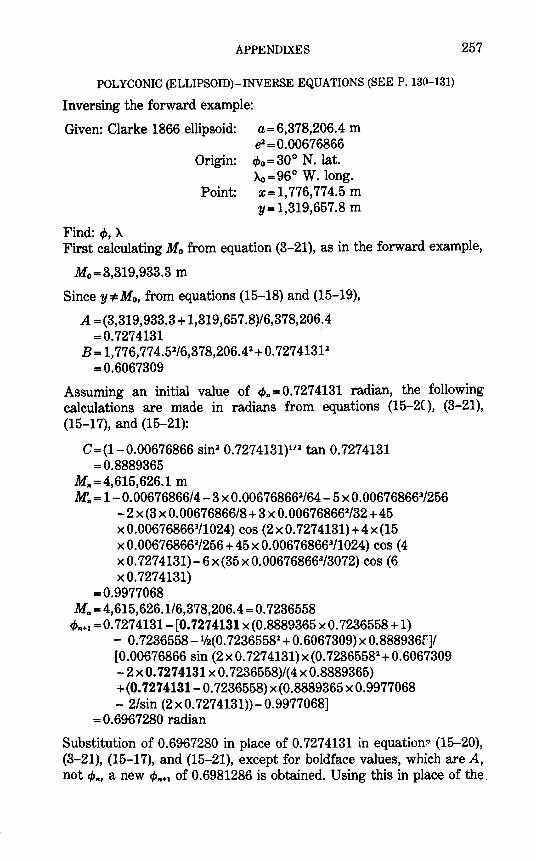
APPENDIXES
POLYCONIC (ELLIPSOID)-INVERSE EQUATIONS (SEE P. 130-131)
Inversing the forward example:
Given: Clarke 1866 ellipsoid: a= 6,378,206.4 m
Find: 4>,).
e1 =0.00676866 Origin: 4>o=30° N. lat.
~=96° W. long. Point: x=1,776,774.5 m
y= 1,319,657.8 m
257
First calculating Mo from equation (3-21), as in the forward example,
Mo = 3,319,933.3 m
Since y:I=M0 , from equations (15-18) and (15-19),
A= (3,319,933.3 + 1,319,657.8)/6,378,206.4 =0.7274131
B = 1, 776,77 4.51/6,378,206.41 + 0. 727 41311
=0.6067309
Assuming an initial value of 4>, = 0. 727 4131 radian, the following calculations are made in radians from equations (15-2C ), (3-21), (15-17), and (15-21):
C=(l-0.00676866 sin1 0.7274131)111 tan 0.7274131 =0.8889365
M,=4,615,626.1 m M, = 1-0.00676866/4-3 X 0.006768661/64- 5 X 0.006768663/256
-2 X (3 X 0.00676866/8 + 3 X 0.006768661/32 + 45 X 0.006768663/1024) COS (2 X 0. 727 4131) + 4 X (15 x0.006768661/256+45x0.006768663/1024) cos (4 X 0. 727 4131)- 6 X (35 X 0.006768663/3072) COS (6 X 0. 727 4131)
=0.9977068 M,. = 4,615,626.1/6,378,206.4 = 0. 7236558
4>n+l = 0. 727 4131- [0. 727 4131 X (0.8889365 X 0. 7236558 + 1) - 0. 7236558 - 112(0. 72365581 + 0.6067309) X 0.888936f]/ [0.00676866 sin (2 x 0. 727 4131) x (0. 72365581 + 0.6067309 -2 xO. 7274131 x 0.7236558)/(4 x0.8889365) +(0. 7274131- 0.7236558)x(0.8889365 x 0.9977068 - 2/sin (2x0.7274131))-0.9977068]
=0.6967280 radian
Substitution of 0.6967280 in place of 0. 727 4131 in equation~ (15-20), (3-21), (15-17), and (15-21), except for boldface values, which are A, not 4>,, a new 4>,+1 of 0.6981286 is obtained. Using this in place of the.

258 MAP PROJECTIONS USED BY THE USGS
previous value results in a third cp,.1 of 0.6981317, which is unchanged by recalculation to seven decimals. Thus,
c/>=0.6981317x 180°111"=40.0000005° =40° N. lat.
From equation (15-22), using the finally calculated C of 0.837~255,
~=[arcsin (1,776,774.5x0.8379255/6,378,206.4)]/sin 40° +( -96°) = -75° =75° W. long.
ORTHOGRAPHIC (SPHERE)-FORWARD EQUATIONS (SEEP. 146-147)
Given: Radius of sphere: R = 1.0 unit Center: c/>1 =40° N. lat.
~ = 100° W. long. Point: c/>=30° N. lat.
~= 110° W. long. Find: x, y In general calculations, to determine whether this point is beyc nd viewing, using equation (5-3),
cos c=sin 40° sin 30°+cos 40° cos 30° cos (-110°+100°) =0.9747290
Since this is positive, the point is within view. Using equations (16-3) and (16-4),
X= 1.0 cos 30° sin ( -110° + 100°) = -0.1503837
y= 1.0 [cos 40° sin 30° -sin 40° cos 30° cos ( -110° + 100°)] = -0.1651911
Examples of other forward equations are omitted, since th~ oblique case applies generally.
ORTHOGRAPHIC (SPHERE)-INVERSE EQUATIONS (SEEP. 147)
Inversing forward example:
Given: Radius of sphere: R = 1.0 unit Center: q,. =40° N. lat.
~o= 100° W. long.
Find: cp, ~
Point: X= -0.1503837 unit Y= -0.1651911 unit
Using equations (16-18) and (16-19),
p =[( -0.1503837)2 +( -0.1651911)2)112
=0.2233906 c=arcsin (0.2233906/1.0)
= 12.9082572°
APPENDIXES
Using equations (16-14) and (16-15),
ct>=arcsin [cos 12.9082572° sin 40° +( -0.1651911 sin 12.9082572° cos 40°/0.22gg906)]
=g0.0000007°, or gooN. lat. if rounding off did not oc~ur. A= -100° +arctan [ -0.150g8g7 sin 12.9082572°/(0.22gg'~06
cos 40° cos 12.9082572° +0.1651911 sin 40° sin 12. 9082572°)]
= -100° +arctan [ -o.ogg594g/0.1905228] = -100° + (- 9.9999964 °) = -109.9999964 °, or 110° W. long. if rounding off did not
occur.
259
Since the denominator of the argument of arctan is positive, no adjustment for quadrant is necessary.
STEREOGRAPHIC (SPHERE)-FORWARD EQUATIONS (SEEP. 158-159)
Given: Radius of sphere: R = 1.0 unit Center: cJ>1 = 40° N. lat.
Ao= 100° W. long. Central scale factor: k0 = 1.0
Point: ct>=goo N. lat. A=75° W. long.
Find: x, y, k Using equations (17-4), (17-2), and (17-g) in order,
k=2xl.0/[1+sin 40° sin goo+cos 40° cos goo cos (-75°+100°)] = 1.0402go4
X= 1.0x 1.0402g04 cos goo sin ( -75° + 100°) = o.g807224 unit
y= l.Ox 1.0402g04 [cos 40° sin goo -sin 40° cos goo cos ( -75° + 100°)]
= -0.126g802 unit
Examples of other forward equations are omitted, since the above equations are general.
STEREOGRAPHIC (SPHERE)-INVERSE EQUATIONS (SEEP. 159)
Inversing forward example:
Given: Radius of sphere: Center:
Central scale factor: Point:
R=l.O unit cl>1 = 40° N. lat. Ao= 100° W. long. k0 = 1.0 x = o.g807224 unit y = - 0.126g802 unit
260 MAP PROJECTIONS USED BY THE USGS
Find:~' A Using equations (16-18) and (17-15),
p = [0.38072242 + (- 0.1263802)2]112 = 0.4011502 units c=2 arctan [0.4011502/(2x l.Ox 1.0)]
= 22.6832261°
Using equations (16-14) and (16-15),
~=arcsin [cos 22.6832261 o sin 40° +( -0.1263802) sin 22.6832261 o cos 40° /0.4011502]
=arcsin 0.5000000=30° =30° N. lat. A= - 100° +arctan [0.3807224 sin 22.6832261 o /(0.4011502
cos 40° cos 22.6832261 o + 0.1263802 sin 40° sin 22.6832261 °)] = -100° +arctan (0.1468202/0.3148570) = -100° + 25.0000013° = -74.9999987° =75° W. long.
except for effect of rounding-off input data. Since the denomjnator of the argument of arctan is positive, no quadrant adjustment is necessary. If it were negative, 180° should be added.
STEREOGRAPHIC (ELLIPSOID)-FORWARD EQUATIONS (SEEP. 160, 162-163)
Oblique aspect:
Given: Clarke 1866 ellipsoid:
or Center:
Central scale factor: Point:
Find: x, y, k From equation (3-1 ),
a= 6,378,206.4 m e2 = 0.00676866 e = 0.0822719
~~ =40° N. lat. >.o= 100° W. long. k0=0.9999 ~=30° N. lat. A=90° W. long.
Xt =2 arctan {tan (45° +40°/2) [(1-0.0822719 sin 40°)/ (1 + 0.0822719 sin 40o)]o.o822719/2}- 90o
= 2 arctan 2.1351882-90° = 39.8085922°
x = 2 arctan {tan (45° + ::\0° /2)[(1- 0.0822719 sin 30°)/ (1 + 0.0822719 sin 30°)]0·0822719'2}- 90°
= 2 arctan 1. 7261956- 90° = 29.8318339°
APPENDIXES
From equation (12-15),
m 1 =cos 40° /(1- 0.00676866 sin2 40°)112
=0.7671179 m=cos 30°/(1-0.00676866 sin2 30°)112
=0.8667591
From equation (17 -27),
A= 2 X 6,378,206.4 X 0.9999 X 0. 7671179/{ cos 39.8085922° [1 x sin 39.8085922° sin 29.8318339° +cos 39.8085922° cos 29.8318339° cos (- 90° + 100°)]}
= 6,450,107.7 m
From equations (17 -24), (17 -25), and (17 -26),
X= 6,450,107. 7 cos 29.8318339° sin (- 90° + 100°) = 971,630.8 m
y= 6,450,107. 7 [cos 39.8085922° sin 29.8318339° -sin 39.8085922° cos 29.8318339° cos ( -90° + 100°)]
= -1,063,049.3 m k= 6,450,107.7 cos 29.8318339°/[6,378,206.4x 0.8667591}
= 1.0121248
Polar aspect with known k0:
Given: International ellipsoid: a= 6,378,388.0 m e2 = 0.00672267
or e= 0.0819919 Center: South Pole c/>1 = 90° S. lat.
261
Ao = 100° W. long. (meridian along pos. Y axis)
Central scale factor: ko = 0.994 Point: c/>=75° S. lat.
X= 150° E. long.
Find: x, y, k Since this is the south polar aspect, for calculations change signs of x,
y, cp, X, and Ao (4>c is not used): Ao= 100° E.long., Q>= 75° N.lat., X= 150° W. long. Using equations (13-9) and (17-33),
t=tan(45° -75°/2)/[(1-0.0819919 sin 75°)/(1+0.0819919 sin 75 0)]0.0819919/2
=0.1325120 p = 2 X 6,378,388.0 X 0.994 X 0.1325120/((1 + 0.0819919)£t+O.Oq199191
X (1- 0.0819919)£1-0.08199191)112 = 1,674,638.5 m
262 MAP PROJECTIONS USED BY THE USGS
Using equations (17-30) and (17-31), changing signs of x andy for the south polar aspect,
X= -1,674,638.5 sin ( -150° -100°) = -1,573,645.4 m
Y= + 1,674,638.5 cos ( -150° -100°) = -572,760.1 m
From equation (12-15),
m= cos 75° /(1- 0.00672267 sin2 75°)112
=0.2596346
From equation (17-32),
k = 1,67 4,638.5/(6,378,388 X 0.2596346) = 1.0112245
Polar aspect with known cf>e not at the pole: Given: International ellipsoid: a= 6,378,388.0 m
&=0.00672267 or e= 0.0819919
Standard parallel: cf>e = 71° S. lat. 'Ao= 100 W. long. (meridian along
pos. Y axis) Point: cp = 75 ° S. lat.
A= 150° E. long.
Find: x, y, k Since cf>e is southern, for calculations change signs of x, y, cf>e, cp, A, and
'Ao: cf>e=71° N.lat., c/>=75° N.lat., A=150° W.long., Ao=100" E. long. Using equation (13-9), t for 75° has been calculated in the r~eceding ex;ample, or
t = 0.1325120
For te, substitute 71° in place of 75 ° in (13-9), and
te = 0.1684118
From equation (12-15),
me=COS 71 °/(1-0.00672267 sin2 71 °)112
=0.3265509
From equation (17-34),
p = 6,378,388.0 X 0.3265509 X 0.1325120/0.1684118 = 1,638,869.6 m
APPENDIXES 263
Equations (17-30), (17-31), and (17-32) are used as in the ~receding south polar example, changing signs of x and y.
X= -1,638,869.6 sin ( -150° -100°) = -1,540,033.6 m
y= + 1,638,869.6 cos ( -150° -100°) = - 560,526.4 m
k = 1,638,869.6/(6,378,388.0 X 0.2596346) =0.9896255
where m is calculated in the preceding example.
STEREOGRAPHIC (ELLIPSOID)-INVERSE EQUATIONS (SEE P. 163-164)
Oblique aspect (inversing forward example):
Given: Clarke 1866 ellipsoid: a= 6,378,206.4 m & = 0.00676866
or e=0.0822719 Center: cp1 =40° N. lat.
Ao= 100° W. long. Center scale factor: k0 =0.9999
Point: x= 971,630.8 m y= -1,063,049.3 m
Find: cp, X From equation (12-15),
m. =cos 40° /(1- 0.00676866 sin1 40°)111
=0.7671179
From equation (3-1), as in the forward oblique example,
Xt = 39.808592.2 t)
From equations (16-18) and (17 -S8),
p = [971,630.81 + ( -1,063,049.3)1)11
1
= 1,440,187.6 m c.=2 arctan [1,440,187.6 cos 39.8085922°/(2x6,378,206.4
X 0.9999 X 0. 7671179)) = 12.9018251°
From equation (17-37),
x=arcsin [cos 12.9018251° sin 39.8085922° +( -1,063,049.3 sin 12.9018251° cos 39.8085922°/1,440,187.6)]
= 29.8318337°
264 MAP PROJECTIONS USED BY THE USGS
Using x as the first trial cp in equation (3-4),
cp = 2 arctan (tan (45° + 29.8318337° /2) x [(1 + 0.0822719 sin 29.8318337°)/(1- 0.0822719 sin 29.8318337°)]0
·082271912
}
-90° = 29.9991438°
Using this new trial value in the same equation for cp, not for x, cp=2 arctan (tan (45° +29.8318337°/2)x[(1+0.0822719
sin 29.9991438°)/(1- 0.0822719 sin 29.9991438°)]0·082271912
}
-90° = 29.9999953 °
Repeating with 29.9999953° in place of 29.9991438°, the next trial cp is
cp = 29.9999997°
The next trial calculation produces the same cp to seven d~cimals. Therefore, this is cp.
Using equation (17 -36),
A= -100° +arctan [971,630.8 sin 12.9018251 o I (1,440,187.6 cos 39.8085922° cos 12.9018251° + 1,063,049.3 sin 39.8085922° sin 12.9018251 °)]
= -100° +arctan (216,946.9/1,230,366.8) = -100° + 10.0000000° = -90.0000000° =90° W. long.
Since the denominator of the arctan argument is positive, no quadrant adjustment is necessary. If it were negative, it would be nece~sary to add or subtract 180°, whichever would place the final A between + 180° and -180°.
Instead of the iterative equation (3-4), series equation (3-5) may be used:
cp = 29.8318337° X 1r/180° + (0.00676866/2 + 5 X 0.006768662/24 + 0.006768663/12) sin (2 x 29.8318337°) + (7 x 0.0067686€2/48 +29x0.006768663/240) sin (4x29.8318337°)+(7 x 0.006768663/120) sin (6 x 29.8318337°)
= 0.5235988 radian = 29.9999997°
Polar aspect with known ko (inversing forward example):
Given: International ellipsoid: a= 6,378,388.0 m e2 = 0.00672267
or e=0.0819919 Center: South Pole cp1 = 90° S. lat.
Ao = 100° W. long. (meridian along pos. Y axis)
Find:¢,~
APPENDIXES
Central scale factor: Point:
k0 =0.994 x= -1,573,645.4 m y= -572,760.1 m
265
Since this is the south polar aspect, change signs as stated in text: For calculation, use cl>c=90°, ~=100° E. long., x=1,573,645.4 m, Y= 572,760.1 m. From equations (16-18) and (17-39),
p = (1,573,645.42 + 572, 760.12)
112
= 1,674,638.5 m t = 1,67 4,638.5 X [(1 + 0.0819919)P•0 ·081991
9 l
(1- 0.0819919)1 1- 0 ·08199191)112/(2 X 6,378,388.0 X 0.994) =0.1325120
To iterate with equation (7 -9), use as the first trial ¢,
¢=90° -2 arctan 0.1325120 = 74.9031975°
Substituting in (7 -9),
¢=90° -2 arctan (0.1325120x[(1-0.0819919 sin 74.903]975°)/ (1 + 0.0819919 sin 74.9031975°)]0 ·0 8 19919'2}
= 74.9999546°
Using this second trial¢ in the same equation instead of 74.9031975°,
cp = 74.9999986°.
The third trial gives the same value to seven places, so, since the sign of ¢must be reversed for the south polar aspect,
cp = -74.9999986°, = 75° S. lat. (disregarding effects of rounding off).
If the series equation (3-5) is used instead of (7 -9), x is first found from (7-13):
x = 90°-2 arctan 0.1325120 = 74.9031975°
Substituting this into (3-5), after converting x to radians fo~ the first term, cp is found in radians and is converted to degrees, then given a reversal of sign for the south polar aspect, giving the same re2ult as the iteration.
From equation (16-16),
~= + 100° +arctan [1,573,645.4/( -572,760.1)] = 100° +( -69.9999995°) = 30.0000005°
266 MAP PROJECTIONS USED BY THE USGS
However, since the denominator of the argument of arctan is ne~ative, 180° must be added to A (added, not substracted, since the numerator is positive), then the sign of A must be changed for the south polar aspect:
A= -(30.0000005° + 180°) =- 210.0000005°
To place this between + 180° and - 180°, add 360°, so
A=+ 149.9999995° or 150° E. long., disregarding effects of rounding off.
Polar aspect with known tPc not at the pole (inversing £1rward example):
Given: International ellipsoid: a= 6,378,388.0 m e2 = 0.00672267
or e= 0.0819919 Standard parallel: tPc = 71° S. lat.
Find: cp, A
A.o= 100° W. long. (meridian along pos. Y axis)
Point: x= -1,540,033.6 m y= -560,526.4 m
Since this is south polar, change signs as stated in text: For calculation, cbc=71° N.lat., A.o=100° E. long., X=1,540,033.6, y=56l.526.4. From equations (13-9) and (12-15), as calculated in the corresJ:onding forward example,
tc=tan (45° -71 °/2)/[(1-0.0819919 sin 71 °)/ (1 + 0.0819919 sin 71 °)]0 ·081991912
=0.1684118 me= cos 71° /(1- 0.00672267 sin2 71 °)112
=0.3265509
From equations (16-18) and (17-40),
p = (1,540,033.62 + 560,526.42)11 2
= 1,638,869.5 m t= 1,638,869.5 X 0.1684118/(6,378,388.0 X 0.3265509) =0.1325120
For the first trial cp in equation (7-9),
cp = 90 ° - 2 arctan 0.1325120 = 74.903197°
APPENDIXES
Substituting in (7 -9),
cf>=90° -2 arctan {0.1325120 [{1-0.0819919 sin 74.903197°)/ (1 + 0.0819919 sin 7 4.903197°)]o.os19919/2}
= 74.9999586°
Replacing 74.903197° with 74.9999586°, the next trial cf> i~·
<I>= 75.0000026°
267
The next iteration results in the same cf> to seven places, S'l changing signs,
cf> = -75.0000026° = 75° S. lat., disregarding effects of r'lunding off.
The use of series equation (3-5) with (7 -13) to avoid iteration follows the same procedure as the preceding example. For A, equation (16-16) is used, calculating with reversed signs:
A=+ 100° +arctan [1,540,033.6/(- 560,526.4)] = 100° + (- 69.9999997°) = 30.0000003°
Since the denominator in the argument for arctan is negative, add 180°:
A= 210.0000003°
Now subtract 360° to place A between + 180° and -180°:
A= -149.9999997°
Finally, reverse the sign to account for the south polar asp~ct:
A=+ 149.9999997° = 150° E. long., disregarding rounding off in the input.
LAMBERT AZIMUTHAL EQUAL-AREA (SPHERE)-FORWARD EQUATIONS (SEEP. 170, 172-173)
Given: Radius of sphere: Center:
Point:
Find: x, y Using equation (18-4),
R=3.0 units c/>1 = 40° N. lat. Ao = 100° W. long.
cf> = 20° S. lat. A= 100° E. long.
268 MAP PROJECTIONS USED BY THE USGS
k' = {2/[1 +sin 40° sin (- 20°) +cos 40° cos (- 20°) cos (100° + 100°)])112
=4.3912175
Using equations (18-2) and (18-3),
X= 3.0x 4.3912175 cos (- 20°) sin (100° + 100°) = - 4.2339303 units
y = 3.0 x 4.3912175 [cos 40° sin (- 20°)- sin 40° cos (- 20°) cos (100° + 100°)]
= 4.0257775 units
Examples for the polar and equatorial reductions, equations (18-5) through (18-16), are omitted, since the above general equations give the same results.
LAMBERT AZIMUTHAL EQUAL-AREA (SPHERE)- INVERSE EQUATIONS (SEEP. 173)
Inversing forward example:
Given: Radius of sphere: Center:
Point:
Find: cp, A
R=3.0 units cpl = 40° N. lat. Ao = 100° W. long. x = - 4.2339303 units Y= 4.0257775 units
Using equations (16-18) and (18-18),
p = [(- 4.2339303)2 + 4.02577752]
112
= 5.8423497 units C= 2 arcsin [5.8423497/(2 x 3.0)]
= 153.6733917°
From equation (16-14),
cp=arcsin [cos 153.6733917° sin 40°+4.0257775 sin 153.6733917° cos 40° /5.8423497]
= -19.9999993° = 20° S. lat., disregarding rounding-off effects.
From equation (16-15),
A= -100° +arctan [ -4.2339303 sin 153.6733917°/ (5.8423497 cos 40° cos 153.6733917° -4.0257775 sin 40° sin 153.6733917°)]
= -100° +arctan [ -1.8776951/( -5.1589246)] = -100° +20.0000005° = -79.9999995 °
Since the denominator of the argument of arctan is negative, ad1180°:
APPENDIXES 269
A= 100.0000005° = 100° E. long., disregarding rounding-off effects.
In polar spherical cases, the calculation of A from equations (16-16) or (16-17) is simpler than the above, but the quadrant adjustment follows the same rules.
LAMBERT AZIMUTHAL EQUAL-AREA (ELLIPSOID)- FORWARD EQUATIONS (SEE P. 173-175)
Oblique aspect:
Given: Clarke 1866 ellipsoid: a= 6,378,206.4 m e2 = 0.00676866
or e= 0.0822719 Center: ¢ 1 = 40° N. lat.
Ao= 100° W. long. Point: ¢=30° N. lat.
A= 110° W. long.
Find: x, y Using equation (3-12),
q=(l- 0.00676866) {sin 30° /(1- 0.00676866 sin2 30°)- [11 (2 x 0.0822719)] In [(1- 0.0822719 sin 30°)/ (1 + 0.0822719 sin 30°)]}
=0.9943535
Inserting ¢ 1 = 40° in place of 30° in the same equation,
q1 = 1.2792602
Inserting 90° in place of 30°,
qp= 1.9954814
Using equation (3-11),
{3 =arcsin (0.9943535/1.9954814) = 29.8877622°
{31 =arcsin (1.2792602/1.9954814) =39.8722878°
Using equation (3-13),
Rq = 6,378,206.4 X (1.9954814/2)112
= 6,370,997.2 m
Using equation (12-15),
m1 =cos 40° /(1- 0.00676866 sin2 40°)112
=0.7671179
270 MAP PROJECTIONS USED BY THE USGS
Using equations (1g-21) and (1g-22),
B= 6,370,997.2 x {2/[1 +sin 39_g722g7go sin 29.gg77622° +cos 39.g722g7go cos 29.gg77622° cos ( -110° + 100°)]}112
= 6,411,606.1 m D = 6,37g,206.4 X 0. 7671179/(6,370,997 .2 cos 39.g722g7g0
)
= 1.0006653
Using equations (1g-19) and (1g-20),
X= 6,411,606.1 x 1.0006653 cos 29.gg77622° sin ( -110° + 100°) = -965,932.1 m
y=(6,411,606.1/1.0006653)[cos 39_g722g7go sin 29.gg77622° -sin 39_g722g7go cos 29.gg77622° cos ( -110° + 100°)]
= -1,056,g14.9 m
Polar aspect:
Given: International ellipsoid: a= 6,37g,3gg_o m e'- = 0.00672267
or e=o.og19919 Center: North Pole .P1 =90° N. lat.
Ao= 100° W. long. (meridian ahng neg. Yaxis)
Point: .P=goo N. lat. A=5° E. long.
Find: q,, A, h, k From equation (3-12),
q=(1-0.00672267) {sin goo/(1-0.00672267 sin1 goo) - [1/(2 x O.og19919)] In [(1- O.Og19919 sin goo)/ (1 + o.og19919 sin goo)]}
=1.96492g3
Using the same equation with 90° in place of goo,
qp = 1.9955122
From equation (12-15),
m=cos goo/(1-0.00672267 sin1 go 0) 111
=0.1742171
Using equations (1g-25), (17-30), (17-31), and (17-32),
p = 6,37g,3gg.0 X (1.9955122 -1.96492g3)111
= 1,115,46g.3 m X= 1,115,46g.3 sin (5°+ 100°)
= 1,077,459.7 m
APPENDIXES
y= -1,115,468.3 cos (5°+ 100°) =288,704.5 m
k = 1, 115,468.3/(6,378,388.0 X 0.17 42171) =1.0038193
h= 1/1.0038193=0.9961952
271
LAMBERT AZIMUTHAL EQUAL-AREA (ELLIPSOID)-INVERSE F~UATIONS (SEEP. 175-177)
Oblique aspect (inversing forward example):
Given: Clarke 1866 ellipsoid: a= 6,378,206.4 m e2 = 0.00676866
Find: ct>, A
or e=0.0822719 Center: cf>t=40° N. lat.
Ao= 100° W. long. Point: X= -965,932.1 m
y= -1,056,814.9 m
Since these are the same map parameters as those used in the forward example, calculations of map constants not affected by cf> arri A are not repeated here.
qp= 1.9954814 P1 = 39.8722878° R,=6,370,997.2 m D = 1.0006653
Using equations (18-30), (18-31), and (18-29),
p = ([ -965,932.1/1.0006653]2 +[1.0006653x( -1,056,814.9)]2 )112
= 1,431,827.1 m c.=2 arcsin [1,431,827.1/(2x6,370,997.2)]
= 12.9039908° q= 1.9954814 [cos 12.9039908° sin 39.8722878°
+ 1.0006653x( -1,056,814.9) sin 12.9039908° cos 39.8722878°/1,431,827.1]
=0.9943535
For the first trial cf> in equation (3-16),
cf> =arcsin (0.9943535/2) = 29.8133914 °
272 MAP PROJECTIONS USED BY THE USGS
Substituting into equation (3-16),
rJ> = 29.8133914 ° + [(1- 0.00676866 sin2 29.8133914 °)2/
(2 COS 29.8133914 °)) X {0.9943535/(1- 0.00676866) -sin 29.8133914 ° /(1- 0.00676866 sin2 29.8133914) + [1/(2 x 0.0822719)] ln [(1- 0.0822719 sin 29.8133914 °)/(1 + 0.0822719 sin 29.8133914 °)]} x 180c I 'If
= 29.9998293 °
Substituting 29.9998293° in place of 29.8133914 ° in the same e~·uation, the new trial rJ> is found to be
rJ> = 30.0000002 °
The next iteration results in no change to seven decimal places; therefore,
<t>=30° N. lat.
Using equation (18-28),
A= -100° +arctan {- 965,932.1 sin 12.9039908°/[1.0006653 X 1,431,827.1 COS 39.8722878° COS 12.9039908° -1.00066532 ( -1,056,814.9) sin 39.8722878° sin 12.9039908 °]}
= -100° +arctan (- 215, 710.0/1,223,352.4) = -100°-9.9999999° = -109.9999999° = 110° W. long.
Since the denominator of the argument for arctan is positive, no quadrant adjustment is necessary.
Polar aspect (inversing forward example):
Given: International ellipsoid: a= 6,378,388.0 m e2 = 0.00672267
Find:</>,}..
or e= 0.0~19919 Center: North Pole <f> 1 =90° N. lat.
>.o = 100° W. long. (meridian along neg. Y axis)
Point: X= 1,077,459. 7 m y=288,704.5 m
First qp is found to be 1.9955122 from equation (3-12), as in the corresponding forward example for the polar aspect. From e~·uations (16-18) and (16-33),
p = (1,077 ,459. 72 + 288, 704.52)
112
= 1,115,468.4 m
APPENDIXES
q= + [1.9955122- (1,115,468.4/6,378,388.0)2]
= 1.9649283
273
Iterative equation (3-16) may be used to find cp. The first trial cp is
cp = arcsin (1. 9649283/2) = 79.2542275°
When this is used in equation (3-16) as in the oblique inve:-:-se example, the next trial cp is found to be
cp = 79 0 97 44304 °
Using this value instead, the next trial is
cp= 79.9999713°
and the next,
cp = 80.0000036 °
The next value is the same, so
cp = 80° N. lat.
From equation (16-16),
A= -100°+arctan [1,077,459.7/(-288,704.5)] = -174.9999978°
Since the denominator of the argument for arctan is ne:trative, add 180°, or
A=5.0000022°=5° E. long.
AZIMUTHAL EQUIDISTANT (SPHERE)-FORWARD EQUATIONS (SEE P. 184-185)
Given: Radius of sphere: Center:
Point:
Find: x, y
R=3.0 units c/>1 = 40° N. lat. Ao = 100° W. long. cp = 20° S. lat. A= 100° E. long.
Using equations (5-3) and (19-2),
COS C=Sin 40° sin ( -20°)+COS 40° COS ( -20°) COS (100° + 100°) = - 0.8962806
C= 153.6733925° k' =(153.6733925° x T/180°)/sin 153.6733925°
=6.0477621
274 MAP PROJECTIONS USED BY THE USGS
Using equations (18-2) and (18-3),
x = 3.0 x 6.04 77621 cos (- 20°) sin (100° + 100°) = - 5.8311398 units
y=3.0x6.0477621 [cos 40° sin (-20°)-sin 40° cos (-20°) cos (100° + 100°)]
= 5.5444634 units
Since the above equations are general, examples of other forward formulas are not given.
AZIMUTHAL EQUIDISTANT (SPHERE)- INVERSE EQUATIONS (SEEP. 185)
Inversing forward example:
Given: Radius of sphere: Center:
Point:
Find: 4>, A
R=3.0 units cl>1 = 40° N. lat. Ao= 100° W. long. X= -5.8311398 units y = 5. 5444634 units
Using equations (16-18) and (19-15),
p = [(- 5.8311398)2 + 5.54446342] 112
= 8.0463200 units C= 8.0463200/3.0
= 2.6821067 radians = 2.6821067 X 180° f1r= 153.6733925°
Using equation (16-14),
¢=arcsin (cos 153.6733925° sin 40° +5.5444634 sin 153.6733925° cos 40°/8.0463200)
= -19.9999999° = 20° S. lat., disregarding effects of rounding off.
Using equation (16-15),
A= -100° +arctan [( -5.8311398) sin 153.6733925°/(8.046f?.OO cos 40° cos 153.6733925°-5.5444634 sin 40° sin 153.6733925°)]
= -100° +arctan [( -2.5860374)/( -7.1050794)] = -100° -arctan 0.3639702 = -80.0000001°
but since the denominator of the argument of arctan is negative, add or subtract 180°, whichever places the final result between + 181° and -180°:
APPENDIXES
A= - go.0000001 o + 1goo = 99.9999999° = 100° E. long., disregarding effects of rounding- of~.
AZIMUTHAL EQUIDISTANT (ELLIPSOID)-FORWARD EQUATIONS (SEE P. 185-189)
Polar aspect:
Given: International ellipsoid: a= 6,37g,3gg.o m e2 = 0.00672267
Center: North Pole cp1 = 90° N. lat.
275
At,= 100° W.long. (meridi~n along neg. Y axis)
Point: cp=goo N. lat. A= 5° E. long.
Find: x, y, k Using equation (3-21),
M=6,37g,3gg.Ox[(l-0.00672267/4-3x0.006722672/64 -5 X 0.006722673/256) X 80° X 1r/1g0o- (3 X 0.00672267/? + 3 x 0.006722672/32 + 45 x 0.006722673/1024) sin (2 x goo) + (15 x 0.006722672/256 + 45 x 0.006722673/1024) sin (4 x goo) - (35 x 0.006722673/3072) sin (6 x goo)]
= g,gg5,403.1 m
Using the same equation (3-21), but with 90° in place of 8~0 ,
Mp = 10,002,2gg.3 m
Using equation (12-15),
m= cos goo /(1- 0.00672267 sin2 go0) 112
=0.1742171
Using equations (19-16), (17-30), (17-31), and (17-32),
p = 10,002,2gg.3-g,ggs,403.1 = 1,116,gg5.2 m
X= 1,116,8g5.2 sin (5°+ 100°) = 1,07g,g2g.3 m
Y= -1,116,gg5.2 cos (5°+ 100°) = 2g9,071.2 m
k= 1,116,gg5.2/(6,37g,3gg.ox 0.1742171) = 1.0050946
276 MAP PROJECTIONS USED BY THE USGS
Oblique aspect (Guam projection):
Given: Clarke 1866 ellipsoid: a= 6,378,206.4 m e2 = 0.00676866
Center: (j> 1 = 13°28'20.87887" N. lat. Ac,= 144°44'55.50254" E. long.
False origin: X0 = 50,000 m y0 =50,000 m
Point: (j>= 13°20'20.53846" N. lat. A= 144°38'07.19265" E. long.
Find: x, y Using equation (19-18), after converting angles to degreer and decimals: ((j>. = 13.472466353°, Ao= 144.748750706°, (j> = 13.33903r461 °, A= 144.635331292°),
x=[6,378,206.4 x(144.635331292° -144.748750706°) cos 13.339038461 °/(1-0.00676866 sin2 13.339038461 °)112
}
xr/180° = -12,287.52 m
Since 50,000 m is added to the origin for the Guam projection,
X= -12,287.52 +50,000.0 = 37,712.48 m
From equation (3-21),
M = 6,378,206.4 X [(1- 0.00676866/4-3 X 0.006768662/64-5 X 0.006768663/256) X 13.339038461° X r/180°- (3 X 0.00676866/8 + 3 X 0.006768662/32 + 45 X 0.006768663
/
1024) sin (2 x 13.339038461 °) + (15 x 0.006768662/256 + 45 x 0.006768663/1024) sin (4 x 13.339038461 °) - (35 x 0.006768663/3072) sin (6 x 13.339038461 °}]
= 1,475,127.96 m
Substituting (j> 1 = 13.472466353° in place of 13.339038461° in the same equation,
M. = 1,489,888. 76 m
Using equation (19-19), and using the x without false origin,
y= 1,475,127.96-1,489,888.76+( -12,287.52)2 tan 13.339038461 o
x (1- 0.00676866 sin2 13.339038461 °)112/(2 x 6,378,206.4) = -14,758.00 m
Adding 50,000 meters for the false origin, y=35,242.00 m
APPENDIXES
Oblique aspect (Micronesia form):
Given: Clarke 1866 ellipsoid: a= 6,378,206.4 m e1 =0.00676866
Center: Saipan Island t/>1 = 15°11'05.6830" N. lat. ~= 145°44'29.9720" E. long.
False origin: Xo=28,657.52 m Yo=67,199.99 m
Point: Station Petosukara tf>= 15°14'47.4930" N. lat.
Find:':"', y A= 145°47'34.9080" E. long.
First convert angles to degrees and decimals:
t/>1 = 15.18491194 ° ~= 145.7416589° t/> = 15.24652583 ° A= 145.7930300°
From equations (4-20a), (4-20), (19-20), and (19-21) in ord~r,
N1 = 6,378,206.4/(1- 0.00676866 x sin1 15.18491194 °)111
= 6,379,687.9 m N = 6,378,206.4/(1- 0.00676866 x sin1 15.24652583°)111
= 6,379,699. 7 m ,Y=arctan [(1-0.00676866) tan 15.24652583°
+0.00676866 x 6379687.9 sin 15.18491194°/ (6,379,699. 7 X COS 15.24652583°))
= 15.2461374°
Az=arctan {sin (145.79303° -145.7416589°)/ [cos 15.18491194 o x tan 15.2461374 o
-sin 15.18491194° x cos (145.79303° -145.741658f 0 )]J =38.9881345°
Since sin Az :1: 0, from equation (19-22a),
s=arcsin [sin (145.79303° -145.7416589°) x cos 15.2461374°/ sin 38.9881345°]
=0.001374913 radians, since sis used only in radians.
From equations (19-23) through (19-27) in order,
G = 0.00676866111 sin 15.18491194 ° /(1- 0.00676866)1/l
= 0.02162319 H=0.00676866111 cos 15.18491194° cos 38.9881345°/
(1-0.00676866)112
= 0.06192519
277
278 MAP PROJECTIONS USED BY THE USGS
C= 6,379,687.9 X 0.001374913 X (1-0.0013749132 X 0.06192f192
X (1- 0.061925192)/6 + (0.00137 49133/8) X 0.02162319 X 0.06192519 X (1- 2 X 0.061925192
) + (0.00137 49134/120) X (0.061925192 X ( 4-7 X 0.061925192
)- 3 X 0.021623192
X (1-7 X 0.061925192))- (0.00137 49135/48) X 0.02162319
X 0.06192519} =8,771.52 m
X=8,771.52x sin 38.9881345° +28,657.52 = 34,176.20 m
y=8,771.52x cos 38.9881345° +67,199.99 =74,017.88 m
AZIMUTHAL EQUIDISTANT (ELLIPSOID)- INVERSE EQUATIO~S (SEE P. 189-192)
Polar aspect (inversing forward example):
Given: International ellipsoid: a=6,378,388.0 m e2 = 0.00672267
Center: North Pole f/> 1 =90° N. lat.
Find: q,, X
Ao = 100° W. long. (meridian along neg. Y axis)
Point: X= 1,078,828.3 m y=289,071.2 m
Using equation (3-21), as in the corresponding forward example,
Mp = 10,002,288.3 m
Using equations (16-18), (19-28), and (8-19),
p = (1,078,828.32 + 289,071.22)
112
= 1,116,885.2 m M = 10,002,288.3-1,116,885.2
= 8,885,403.1 m p.=8,885,403.1/[6,378,388.0x(1-0.00672267/4-3x0.006722672/64
-5 X 0.006722673/256)) = 1.3953965 radians = 1.3953965x 180°/r=79.9503324°
Using equations (3-24) and (3-26),
e. =[1-(1-0.00672267)112]/[1 +(1-0.00672267)112]
=0.0016863 q, = 1.3953965 radians+ (3 x 0.0016863/2-27 x 0.0016863' /3'i.'
sin (2 x 79.9503324 °) + (21 x 0.00168632/16-55 x0.00168634/32) sin (4x79.9503324°)+(151 x 0.00168633/96) sin (6 x 79.9503324 °)
APPENDIXES
= 1.3962634 radians = 1.3962634 x 180°/r= 79.9999999° = 80° N. lat., rounding off.
Using equation (16-16),
>-= -100° +arctan [1,078,828.3/( -289,071.2)] = -100° -74.9999986° + 180° = 5.0000014 ° =5° E. long., rounding off.
279
The 180° is added because the denominator in the argument for arctan is negative.
Oblique aspect (Guam projection, inversing forward examr1e):
Given: Clarke 1866 ellipsoid: a=6,378,206.4 m e2 = 0.00676866
Center: c/>1 = 13.472466353° N. lat >.o=144.748750706° E.lo'lg.
False origin: Xo=50,000 m Yo=50,000 m
Find: c/>,).
Point: x=37,712.48 m y=35,242.00 m
First subtract 50,000 m from x andy to relate them to actual projection origin: x=-12,287.52 m, Y=-14,758.00 m. Calculation of M. from equation (3-21) is exactly the same as in the forward exan1ple, or
M. = 1,489,888. 76 m
From equation (19-30), the first trial M is found from rn assumed cP =ct>.:
M = 1,489,888.76+( -14,758.00)-( -12,287.52)2 tan 13.472466353° x (1- 0.00676866 sin2 13.472466353°)112/(2 x 6,378,206.4)
= 1,475,127.92 m
Using equation (8-19) and the above trial M,
p.= 1,475,127.92/[6,378,206.4x(1- 0.00676866/4-3 x 0.~'>6768662/ 64-5 X 0.006768663/256)]
= 0.2316688 radian
Using equation (3-24),
e.= [1- (1- 0.00676866)112]/[1 + (1- 0.00676866)112]
=0.0016979
280 MAP PROJECTIONS USED BY THE USGS
Using equation (3-26) in radians, although it could be converted to degrees,
cp = 0.2316688 + (3 X 0.0016979/2-27 X 0.00169793/32) sin (2 x 0.2316688) + (21 x 0.00169791/16-55 x 0.00169794/32) sin ( 4 x 0.2316688) + (151 x0.00169793/96) sin (6x0.2316688)
= 0.2328101 radian = 0.2328101 X 180°/7r= 13.3390381°
If this new trial value of cp is used in place of c/>1 in equation (19-30), a new value of M is found:
M=1,475,127.95 m
This in turn, used in (8-19), gives
p. = 0. 2316688 radian
and from (3-26)
cp = 13.3390384 °
The third trial, through the above equations and starting with this value of cp, produces no change to seven decimal places. Thus, this is the final value of cp. Converting to degrees, minutes, and seconds,
cp = 13°20'20.538" N. lat.
Using equation (19-31) for longitude,
A= 144.748750706° +[( -12,287.52)x(1-0.00676866 sin1 13.3390384 °)111/(6,378,206.4 cos 13.3390384 °)] x 180c l1r
= 144.6353313° = 144 °38'07.193" E. long.
Oblique aspect (Micronesia form, inversing forward example):
Given: Clarke 1866 ellipsoid: a= 6,378,206.4 m e2 = 0.00676866
Center: Saipan Island c/>1 = 15.18491194 ° N. lat.
Find: c/>, A
Ao=145.7416589° E. long. False origin: X0 =28,657.52 m
Yo=67,199.99 m Point: x = 34,176.20 m
y=74,017.88 m
From equations (19-32) through (19-41) in order,
C= ((34,176.20-28,657.52)1 +(74,017.88 -67,199.99)1)111
=8,771.51 m
APPENDIXES
Az =arctan [(34, 176.20- 28,657.52)/(7 4,017.88- 67,199.99)] =38.9881292°
N1 = 6,378,206.4/(1- 0.00676866 sin2 15.18491194 °)112
=6,379,687.9 m A= -0.00676866 cos2 15.18491194° cos2 38.9881292°/
(1- 0.00676866) = -0.003834730
B=3x0.00676866x(l+0.003834730) sin 15.18491194° cos 15.18491194° X COS 38.9881292°/(1-0.00676866)
= 0.004032465 D = 8, 771.51/6,379,687.9
= 0.00137 4913
281
E = 0.00137 4913 + 0.003834 730 X (1- 0.003834 730) X 0.00137 49133/6 -0.004032465 X (1- 3 X 0.003834 730) X 0.00137 49134/24
= 0.00137 4913. This is in radians for use in equation (19-38).
For use as degrees in equations (19-39) and (19-40),
E= 0.001374913 X 180°11r=0.07877669° F = 1 + 0.003834 730 X 0.00137 49132/2-0.004032465
X 0.0013749133/6 = 1.000000004
,P=arcsin (sin 15.18491194° cos 0.07877669° + cos 15.18491194° x sin 0.07877669° cos 38.9881292°)
= 15.246137 4 ° A= 145.7416589° + arcsin (sin 38.9881292° sin 0.07877f~9°/
cos 15.246137 4 °) = 145.7 416589° + 0.0513711° = 145.7930300° = 145°47'34.908" E. long.
cJ>=arctan [(1-0.00676866xl.000000004 sin 15.184911g4°/ sin 15.246137 4 °) x tan 15.246137 4 ° /(1- 0.00676866)]
= 15.2465258° = 15°14'47.493" N. lat.
SPACE OBLIQUE MERCATOR (SPHERE)-FORWARD EQUATIONS (SEEP. 198-200)
Given: Radius of sphere: R=6,370,997.0 m Landsat orbit: i=99.092°
PiP1 = 18/251 Path= 15
Point: q, = 40° N. lat. A= 73° W. long.
Find: x, y for point taken during daylight northern (first) q·.tadrant of orbit.
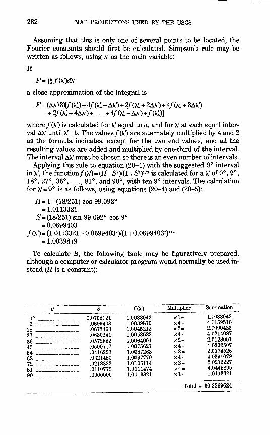
282 MAP PROJECTIONS USED BY THE USGS
Assuming that this is only one of several points to be located, the Fourier constants should first be calculated. Simpson's rule may be written as follows, using A.' as the main variable:
If
F= I!f(A.')dA'
a close approximation of the integral is
F = (~A.' /3)[{ ('A~)+ 4f ('A~ + .:l'A ~ + 2/ ('A~ + 2~A.') + 4f (~ + 3~A.') + 2/ (~ + 4~A.') + ... + 4f ('A~- ~X')+ f ('AD]
where f ('A~ is calculated for X' equal to a, and for A.' at each eqmll interval.:lX' until X'=b. The valuesf(X~ are alternately multiplied by 4 and 2 as the formula indicates, except for the two end values, and all the resulting values are added and multiplied by one-third of the interval. The interval.:lX' must be chosen so there is an even number of ill tervals.
Applying this rule to equation (20-1) with the suggested 9° interval in A.', the function f (A.')= (H-8 2)/(1 + 8 2) 112 is calculated for a A.' o-t 0 °, 9 °, 18°, 27°, 36°, ... , 81 o, and 90°, with ten 9° intervals. The cal~ulation for A.'= 9° is as follows, using equations (20-4) and (20-5):
H= 1-(18/251) cos 99.092° = 1.0113321
S = (18/251) sin 99.092° cos 9° =0.0699403
/(A.')= (1.0113321- 0.06994032)/(1 + 0.06994032)112
= 1.0039879
To calculate B, the following table may be figuratively p:":'epared, although a computer or calculator program would normally be used instead (H is a constant):
)..' s f('A1 Multiplier Surmation
oo -------------- 0.0708121 1.0038042 x1= 1.(038042
9 --------------- .0699403 1.0039879 x4= 4.059516
18 --------------- .0673463 1.0045212 x2= 2.('090423
27 --------------- .0630941 1.0053522 x4= 4.(\214087
36 --------------- .0572882 1.0064001 x2= 2.(\128001
45 --------------- .0500717 1.0075627 x4= 4.(\302507
54 --------------- .0416223 1.0087263 x2= 2.0174526
63 --------------- .0321480 1.0097770 x4= 4.0391079
72 --------------- .0218822 1.0106114 x2= 2.0212227
81 --------------- .0110775 1.0111474 x4= 4.0445895
90 --------------- .0000000 1.0113321 x1= 1.0113321
Total = 30.2269624
APPENDIXES 283
To convert to B, again referring to equation (20-1) and remaining in degrees for the final multipliers, since they cancel,
B = (2/180°) X (9° /3) X 30.2269624 = 1.0075654
This is the Fourier coefficient B for equation (20-6) with 'A' in radians. To use 'A' in degrees, multiply B by r/180°:
B = 1.0075654 x r/180 =0.017585334
Calculations of A .. and c .. are similar, except that the calculations of the function involve an additional trigonometric term at eac.h step. For example, to calculate C3 for 'A'= 9°, using equation (20-3) and the S found above from equation (20-5),
./{'A~= [S/(1 + 81)
111] cos 3'A'
= [0.0699403/(1 + 0.06994031) 111] COS (3 X 9°) = 0.06216542
The sums for A .. corresponding to 30.2269624 forB are as follows:
for A1:- 0.0564594 for A4 : 0.000041208
To convert to the desired constants,
A 1 = [ 4/(180° X 2)] X (9° /3) X (- 0.0564594) = -0.00188198
A 4 = [4/(180° x 4)] x(9° /3)x (0.000041208) = 0. 0000006868
The sums for C .. :
for C1 : 1.0601909 for C3:- 0.0006626541
To convert,
C1 = [ 4 X (1.0113321 + 1)/(180° X 1)] X (9° /3) X (1.0601909) =0.1421597
C3 = [4X (1.0113321 + 1)/(180° X 3)] X (9°/3)x(- 0.0006626541) = -0.0000296182
These constants, rounded to seven decimal places except forB, will be used below:
Using equation (20-11),
Ao = 128.87° - (3.90° /251) X 15 = 107.36°
284 MAP PROJECTIONS USED BY THE USGS
To solve equations (20-8) and (20-9) by iteration, determine }..'p from equation (20-12) and the discussion following the equation, with N = 0:
}..'p=90° x(4x0+2-1) =90°
Then 'At = -73°-107.36° +(18/251)x 90° p •
= -173.9058167° cos 'At =- 0.9943487
p
Using }..'p as the first trial value of}..' in equation (20-9), usir~ extra decimal places for illustration:
'At= -73°-107.36° +(18/251)x 90° = -173.9058167°, as before.
Using equation (20-8),
}..'=arctan [cos 99.092° tan (-173.9058167°) +sin 99.092(' tan 40° /cos ( -173.9058167°)]
= -40.36910525°
For quadrant correction, from the discussion following equation (20-12), using the sign of cos 'At as calculated above,
p
}..' = -40.36910525° + 90°-90° sin 90° x ( -1) = -40.36910525° + 180° = 139.6308947°
This is the next trial}..'. Using equation (20-9),
'At= -73°-107.36° +(18/251)x 139.6308947° = -170.3466291°
Substituting this value of 'Ar in place of -173.9058167° in equation (20-8),
}..' = - 40.9362858°
The same quadrant adjustment applies:
}..' = -40.9362858° + 180° = 139.0637142°
Substituting this in equation (20-9),
At= -170.3873034°
and from equation (20-8),
}..' = 139.0707998°
From the 4th iteration,
At= -170.3867952° A'= 139.0707113°
From the 5th iteration,
At= -170.3868016° A'= 139.0707124 o
From the 6th iteration,
At= -170.3868015° A'= 139.0707124 o
APPENDIXES 285
Since A' has not changed to seven decimal places, the last it.eration is taken as the final value. Using equation (20-10), with the final value of
A" <P' = arcsin [cos 99.092 o sin 40 o - sin 99.092° cos 40 ° sin
( -170.3868015°)] = 1.4179606°
From equation (20-5),
8=(18/251) sin 99.092° cos 139.0707124° = -0.0534999
From equations (20-6) and (20-7),
X= 6,370,997x {0.017585334x 139.0707124° +( -0.0018821) sin (2x 139.0707124°)+0.0000007 sin (4x 139.070712-:1,0
)
- [- 0.0534999/(1 + (- 0.0534999)2) 112] In tan ( 45 ° + 1.4179606 ° /2)}
= 15,601,233.74 m y= 6,370,997x{0.1421597 sin 139.0707124° +( -0.000029~)
sin (3 x 139.0707124 °) + [1/(1 + (- 0.0534999)2) 112]
In tan ( 45 o + 1.4179606 o /2)} = 750,650.37 m
SPACE OBLIQUE MERCATOR (SPHERE)- INVERSE EQUATIONS (SEE P. 200-202)
Inversing forward example:
Given: Radius of sphere: R=6,370,997.0 m Landsat orbit: i= 99.092°
P21P1 = 18/251 Path=15
286 MAP PROJECTIONS USED BY THE USGS
Point:
Find: cp, A
x= 15,601,233.74 m y=750,650.37 m
Constants A1 , A 4 , B, C11 C3 , and Ao are calculated exactly and have the same values as in the forward example above. To solve equation (20-15) by iteration, the first trial A' is x/BR, using the value of B for A' in degrees in this example:
A'= 15,601,233. 74/(0.017585334 X 6370997.0) = 139.2518341°
Using equation (20-5) to findS for this trial A',
S = (18/251) sin 99.092° cos 139.2518341° = -0.0536463
Inserting these values in the right side of equation (20-15),
A'= {15,601,233.74/6,370,997.0+(- 0.0536463) x 750,650.37/6,370,997.0- (- 0.0018820) sin (2 x 139.2f18341 °) -0.0000007 sin (4x 139.2518341 °)-(- 0.0536463) x [0.1421597 sin 139.2518341 o + (- 0.0000296) sin (3 x 139.2518341 °)]}/0.017585334
= 139.0695675°
Substituting this new trial value of A' in (20-5) for a newS, then both in (20-15) for a new A', the next trial value is
A'= 139.0707197° The fourth value is
A'= 139.0707124 o
and the fifth does not change to seven decimal places. Therefo~e, this A' is the final value. The corresponding S last calculated from (20-5) is
S = (18/251) sin 99.092° cos 139.0707124 o
= -0.0534999
Using equation (20-16),
ln tan (45° +cJ>'/2)=[1 +( -0.0534999)2]
112 x[750650.37/ 6370997.0-0.1421597 sin 139.0707124° - (- 0.0000296) sin (3 x 139.0707124 °)]
=0.02475061
tan (45o +cJ>'/2)=eo.ol47so6t =1.0250594
45 ° + cp' /2 =arctan 1. 0250594 =45. 7089803°
c!>'=2x(45.7089803° -45°) = 1.4179606°
APPENDIXES
Using equation (20-13),
~=arctan [(cos 99.092° sin 139.0707124°- sin 99.092° tan 1.4179606 °)/cos 139.0707124 °]- (18/251) 139.0707124 ° + 107.36°
=arctan [ -0.1279654/( -0.7555187)]+97.3868015° =9.6131985° +97.3868015° = 107.0000000°
287
Since the denominator of the argument of arctan is negativ~, and the numerator is negative, 180° must be subtracted from~' or
~= 107.0000000°-180° = -73.0000000° = 73° W. long.
Using equation (20-14),
4> =arcsin (cos 99.092 ° sin 1.4179606 ° + sin 99.092 ° cos 1.4179606° sin 139.0707124 °)
= 40.0000000° =40° N. lat.
For groundtrack calculations, equations (20-17) through (20-20) are used, given the same Landsat parameters as above for R, i, P1/P., and path 15, with ~o= 107.36°, and 4>=40° S. lat. on the daylight (descending) part of the orbit. Using equation (20-17),
~,=arcsin [sin (- 40°)/sin 99.092°] = -40.6145062°
To adjust for quadrant, subtract from 180°, which is the ~, of the descending node:
~'= 180° -( -40.6145062°) = 220.6145062°
Using equation (20-18),
~=arctan [(cos 99.092° sin 220.6145062°)/cos 220.6145062°] -(18/251)x220.6145062° + 107.36°
=arctan [0.1028658/( -0.7591065)] + 91.5390394° = 83.8219462°
Since the denominator of the argument for arctan is negative, add 180°, but 360° must be then subtracted to place ~ between -+ 180° and -180°:
~ = 83.8219462 + 180°- 360° = - 96.1780538 ° = 96°10'40.99" W. long.
If~ is given instead, with the above ~ used for the example, equations (20-19) and (20-9) are iterated together using the same type of initial
288 MAP PROJECTIONS USED BY a'HE USGS
trial 'A' as that used in the forward example for equations (20·-8) and (20-9). In this case, as described following equation (20-12), 'A'p is 270°, but this is only known from the final results. If 'A'p = 90° is choe·en, the same answer will be obtained, since there is considerable overlap in actual regions for which two adjacent 'A'p's may be used. If 'A'p = 450° is chosen, the 'A' calculated will be about 487.9°, or the position on the next orbit for this 'A. Using 'A'p = 270° and the equation for Atp fo11owing equation (20-12),
'Arp= -96.1780538°-107.36° +(18/251)x270° = -184.1755040°
for which the cosine is negative. From equation (20-9), the first trial At is the same as Atp· From equation (20-19),
'A'= arctan [tan ( -184.1755040°)/cos 99.092°] = 24.7970120°
For quadrant adjustment, using the procedure following (20-12),
'A'= 24.7970120 + 270°- 90° sin 270° x ( -1) = 204.7970120°
where the ( -1) takes the sign of cos Atp•
Substituting this as the trial 'A' in (20-9),
At= -96.1780538°-107.36° +(18/251)x204.7970120° = -188.8514155°
Substituting this in place of -184.1755040° in (20-19),
'A'= 44.5812628°
but with the same quadrant adjustment as before,
'A'= 224.5812628°
Repeating the iteration, successive values of 'A' are
'A'= 219.5419815 °, then = 220.8989682°, then = 220.5386678°, then = 220.6346973°, then = 220.6091287°, then = 220.6159384 °, etc.
After a total of about 16 iterations, a value which does not ch~.nge to seven decimal places is obtained:
'A'= 220.6145063°
APPENDIXES 289
Using equation (20-20),
f/>=arcsin (sin 99.092° sin 220.6145063°) = -40.0000000° =40° S. lat.
SPACE OBLIQUE MERCATOR (ELLIPSOID)-FORWARD EQUAT~0NS (SEE P. 203-207)
While equations are given for orbits of small eccentricity, th~ calculations are so lengthy that examples will only be given for the circular Landsat orbit, thus eliminating or simplifying several of the equations given in the text.
Given: Clarke 1866 ellipsoid: a= 6,378,206.4 m e2 = 0.00676866
Landsat orbit: i= 99.092° P2/P1 = 18/251
Ro=7,294,690.0 m Path=15
Point: 4> = 40° N. lat. A=73° W. long.
Find: x, y for point taken during daylight northern (first) qu~.drant of orbit.
The calculation of Fourier constants for the map follows the same basic procedure as that given for the forward example for the spherical form, except for greater complications in computing each swp for the Simpson's numerical integration. The formula for Simpson's rule (see above) is not repeated here, but an example of calculation of e. function f (A'1 for constant A2 at A"= 18 ° is given below, as represented in equation (20-23).
f (A")= [ (HJ-S2)/(J2 + 8 2)
112] cos 2A"
Using equations (20-27) through (20-30) in order,
J =(1-0.00676866)3
=0.9798312 W =[(1-0.00676866 cos2 99.092°)2/(1-0.00676866)2]-1
=0.0133334 Q = 0.00676866 sin2 99.092° /(1- 0.00676866)
=0.0066446 T=0.00676866 sin2 99.092° x (2-0.00676866)/(1-0.00676866)2
=0.0133345
290 MAP PROJECTIONS USED BY THE USGS
Using equations (20-37) and (20-38), remembering that L' = 1.0 for the circular orbit (as can be readily determined from (20-39) wit}' e = 0),
8=(18/251) x 1.0 sin 99.092° cos 18° x[(1 +0.0133345 sin1 18°)/(1 + 0.0133334 sin1 18°) (1 + 0.0066446 sin1 18('))111
=0.0673250 H = [(1 + 0.0066446 sin1 18°)/(1 + 0.0133334 sin1 18°)]111
x [(1+0.0133334 sin1 18°)/(1+0.0066446 sin1 18°)1
- (18/251) X 1.0 COS 99.092°] = 1.0110133
Calculating the function j{'A.'~ as given above, j{)..")= ((1.0110133 X 0.9798312- 0.06732501)/(0.97983121
+ 0.06732501)
111] COS (2 X 18°)
=0.8122693
In tabular form, using 9° intervals in )..", the calculation of A 1 proceeds as follows, integrating only to 90° for the circular orbit:
'A" H s f('A") Multiplier Srmmation
0° _________ 1.0113321 0.0708121 1.0035971 x1= 1.0035971 9 __________ 1.0112504 0.0699346 0.9545807 x4= 3.8183229
18 __________ 1.0110133 0.0673250 0.8122693 x2= 1.6245386 27 __________ 1.0106439 0.0630509 0.5904356 x4= 2.3617425 36 ---------- 1.0101782 0.0572226 0.3106003 x2= 0.6212007 45 ---------- 1.0096617 0.0499888 0.0000000 x4= 0.0000000 54 __________ 1.0091450 0.0415321 -0.3110197 x2= -0.6220394 63 __________ 1.0086787 0.0320636 -0.5919529 x4= -2.3678116 72 __________ 1.0083085 0.0218167 -0.8151437 x2= -1.6302874 81 ---------- 1.0080708 0.0110417 -0.9585531 x4= -3.8342122 90 ---------- 1.0079888 0.0000000 -1.0079888 x1= -1.0079888
Total= -0.0329376
To convert to A 1 , referring to equation (20-23), but multiplying by 4 because of the single-quadrant integration,
A1 =[41(180° x2)]x(9°/3)x( -0.0329376) = -0.0010979
Similar calculations of A 4 , B 1 , c., and C3 lead to the values given in the text following equation (20-73a):
B 1 = 0.0175544891 for ).." in degrees A4 = -0.0000013 c.= 0.1434410 C3 =0.0000285
Since the calculations of j" and m" are not necessary for calculation of x andy from cp and 'A., or the inverse, and are also lengthy, they will be
APPENDIXES 291
omitted in these examples. The examples given will, however4, assist in
the understanding of the text concerning their calculations. The other general constant needed is~, determined from (20-11), as in the forward spherical formulas and example:
~ = 128.87° - (360° /251) X 15 = 107.36°
For coordinates of the specific point, equations (20-45) ari (20-46) are iterated together, replacing (L +-y) with 'A" in (20-46) for tl'~ circular orbit. Except for the additional factor of (1- e1) in (20-45), the procedure is identical to the forward spherical example for solvng (20-8) and (20-9). The calculations of "A'p and the first trial A, are idertical with that example since <1> and 'A have been made the same. The sign of cos A,p is also negative.
A1p=90° 'A,= -173.9058167°
Using equation (20-45),
"A"=arctan [cos 99.092° tan ( -173.9058167°)+(1-0.0067~~66) sin 99.092° tan 40°/cos ( -173.9058167°)]
= -40.1810005°
For quadrant correction,
'A"= -40.1810005°+90°-90° sin 90°X(-1) = 139.8189995°
Successive iterations give
(2) 'A,= -170.3331395° 'A"= 139.2478915°
(3) 'A,= -170.3740954° 'A"= 139.2550483°
(4) 'A,= -170.3735822° 'A"= 139.2549587°
(5) 'A,= -170.3735886° 'A"= 139.2549598°
(6) 'A,= -170.3735885° 'A"= 139.2549598°
These last values do not change within seven decimal places in subsequent iterations.
Using equation (20-49) with the final value of A,,
</>"=arcsin {[(1- 0.00676866) cos 99.092° sin 40°- sin 99.092° cos 40° sin ( -170.3735885°)]/(1- 0.00676866 sin2 40°)112}
= 1.4692784 °
292 MAP PROJECTIONS USED BY THE USGS
From equation (20-37), using 139.2549598° in place of 18° in th~ example for calculation of Fourier constants,
S= -0.0535730
From equations (20-43a) and (20-44a),
X= 6,378,206.4 X {0.0175544891 X 139.2549598° + (- 0.0010979) sin (2x 139.2549598°)+( -0.0000013) sin (4x 139.25495fqo) - [ -0.0535730/(0.97983122 +(- 0.0535730)2
)l'2
] ln tan (45° + 1.4692784 ° /2)}
= 15,607,700.94 m y = 6,378,206.4x {0.1434410 sin 139.2549598° + 0.0000285
sin (3 x 139.2549598°) + [0.9798312/(0.97983122
+( -0.0535730)2) 112] ln tan (45° + 1.4692784°/2)} = 760,636.33 m
For calculation of positions along the groundtrack for a circular orbit, these examples use the same basic Landsat parameters as those in the preceding example, except that ¢ = 40° S. lat. on the daylight (descending) part of the orbit. To find A', cpll is first calculated from equation (20-57):
c/>g=( -40°)-arcsin (6,378,206.4x0.00676866 sin ( -40°) coF (- 40°)/[7 ,294,690.0 x (1- 0.00676866 sin2
(- 40°))1'
2]
= -40° -( -0.1672042°) = -39.8327958°
From equation (20-56),
A'= arcsin [sin (- 39.8327958°)/sin 99.092°] = -40.4436361°
To adjust for quadrant, since the satellite is traveling south, subtract from 1/z x 360°:
A1 = 180°-(- 40.4436361 °) = 220.4436361°
Using equation (20-59), replacing (L + 'Y) with A' for the circular orbit,
A= arctan [(cos 99.092° sin 220.4436361 °)/cos 220.4436361 °] -(18/251)x220.4436361 o + 107.36°
=arctan [0.1025077/( -0.7610445)]+91.5512930° = 83.8800995 °
Since the denominator of the argument for arctan is negat:ve, add 180°, but 360° must also be subtracted to place A between + 180° and -180°:
A= 83.8800995° + 180°-360° =- 96.1199005° =96°07'11.64" W. long.
APPENDIXES 293
If A is given instead, with the above A used in the exampl€, equations (20-19) and (20-46) are iterated together, with A' in place of (L +-y) in the latter for the circular orbit. The technique is the same as that used previously for solving (20-8) and (20-9) in the forward sphe-.oical example. See also the discussion for the corresponding spherical groundtrack example, using equations (20-19) and (20-9), near the end of the inverse example. Since the formulas for the circular orbit ar~ the same for ellipsoid or sphere for this particular calculation, the various iterations are not shown here. With A= -96.1199005°, A' is found to be 220.4436361 o. To find the corresponding cJ> from equation (20-61), a trial cJ>=arcsin (sin 99.092° sin 220.4436361°)= -39.8327;lfi8° is inserted:
cJ> =arcsin (sin 99.092° sin 220.4436361 °) + arcsin {6,378,206.4 x 0.00676866 sin (- 39.832795F0
)
COS (- 39.8327958°)/(7,294,690.0 X (1- 0.00676866 sin2
(- 39.8327958°))1'
2])
= -39.9998234°
Substituting -39.9998234 o in place of -39.8327958° in the same equation, a new value of cJ> is obtained:
cJ>= -39.9999998°
With the next iteration,
cJ>= -40.0000000°
which does not change to seven decimal places. Thus,
c/>=40° S. lat.
SPACE OBLIQUE MERCATOR (ELLIPSOID)-INVERSE EQUATIONS (SEE P. 207-210)
This example is limited to the circular Landsat orbit, using the parameters of the forward example.
Inversing forward example:
Given: Clarke 1866 ellipsoid: a= 6,378,206.4 m e2 =0.00676866
Landsat orbit: i=99.092° PiP1 = 18/251
R0 =7,294,690.0 m Path= 15 (thus Ao= 107.36° as in
forward example) Point: x= 15,607,700.94 m
y=760,636.33 m
294 MAP PROJECTIONS USED BY THE USGS
Find: cp, A All constants J, W, Q, T, A"' B., and C"' as calculated in the forward
example, must be calculated or otherwise provided for use for inverse calculations.
To find A" from equation (20-68a) by iteration, the procedure is identical to that given for (20-15) in the inverse spherical example, except for the use of different constants. For the initial A" =xlaB11
A"= 15,607, 700.94/(6,378,206.4 X 0.0175544891) = 139.3965968°
Using equation (20-37) to findS for this value of A",
S = (18/251) x 1.0 sin 99.092° cos 139.3965968° x [(1 + 0.0133~45 sin2 139.3965968°)/(1 + 0.0133334 sin2 139.3965968°)(1 + 0.0066446 sin2 139.3965968°)]112
= -0.0536874
Inserting these values into (20-68a},
A"= {15,607, 700.94/6,378,206.4+ (- 0.0536874/0.9798312) x(760,636.33/6,378,206.4)-( -0.0010979) sin (2 x 139.3965968°)-( -0.0000013) sin (4x 139.3965968°) -( -0.0536874/0.9798312)x[0.1434410 sin 139.3965968° + 0.0000285 sin (3 x 139.3965968°)]}/0.0175544891
= 139.2539963°
Substituting this new trial value of A" into (20-37) for a newS, then both into (20-68a), the next trial value is
A"= 139.2549663°
and the fourth trial value is
A"= 139.2549597°
The fifth trial value is
A"= 139.2549598°
which does not change with another iteration to seven decimal places. Therefore, this is the final value of A". The correspondini!· S last calculated from (20-37) using this value of A" is -0.0535730. Using equation (20-69a),
ln tan (45° +cp"/2)=[1 +( -0.0535730}2/0.97983122]
112
x [760,636.33/6,378,206.4- 0.1434410 sin 139.2549598°-0.0000285 sin (3 x 139.2549598°)]
=0.0256466
APPENDIXES
tan ( 45 o + cl>" /2) = eo.o2s6466 = 1.0259783
45 ° + cl>" /2 =arctan 1. 0259783 =45.7346392°
cp" = 2 X ( 45.7346392 ° - 45 °) = 1.4692784 °
Using equations (20-65), (20-64), and (20-63) in order,
U = 0.00676866 cos2 99.092° /(1- 0.00676866) =0.0001702
V = {[1- sin2 1.4692784 ° /(1- 0.00676866)] cos 99.092° sin 139.2549598°- sin 99.092° sin 1.4692784 ° x [(1 + 0.0066446 sin2 139.2549598°) x (1- sin2 1.46927,<")d: 0 )
-0.0001702 sin2 1.4692784 °)112}1 [1- sin2 1.4692784 ° (1 + 0.0001702)]
= -0.1285013 A,=arctan ( -0.1285013/cos 139.2549598°)
=arctan [ -0.1285013/( -0.7576215)] =9.6264115°
295
Since the denominator of the argument for arctan is negative, and the numerator is negative, subtract 180 °:
A,= 9.6264115° -180° = -170.3735885°
Using equation (20-62), with A" in place of (L +"f) for the circ·1lar orbit,
A= -170.3735885° -(18/251)x 139.2549598° + 107.36° = -73.0000000° =73° W. long.
Using equation (20-66),
cJ> =arctan {[tan 139.2549598° cos ( -170.3735885 °) -cos 99.092° sin ( -170.3735885°)]/[(1-0.00676866) sin 99.092°]}
= 40.0000000° =40° W. lat.
VANDER GRINTEN (SPHERE)-FORWARD EQUATIONS (SEEP. 214)
Given: Radius of sphere: Central meridian:
Point:
R=l.O unit Ao=85° W. long.
cJ> = 50° S. lat. A= 160° W. long.
296 MAP PROJECTIONS USED BY THE USGS
Find: x, y From equations (21-6), (21-3), (21-4), (21-5), and (21-6a) in o ... der,
8=arcsin l2x( -50°)/180° I =arcsin 0.5555556 = 33.7 489886 °
A= 1/21180° /[( -160°)- (- 85 °)]- [( -160°)- (- 85 °)]/180° I = 1!2! - 2.4oooooo-<- 0.4166667) 1 =0.9916667
G=cos 33.7489886°/(sin 33.7489886° +cos 33.7489886° -1) =2.1483315
P=2.1483315x(2/sin 33.7489886° -1) =5.5856618
Q=0.99166672 +2.1483315=3.1317342
From equation (21-1),
X= -7r X 1.0 X {0.9916667 X (2.1483315- 5.58566182)
+ (0.99166672 X (2.1483315- 5.58566182)
2
- (5.58566182 + 0.99166672) X (2.14833152
- 5.58566182)]
112)/
(5.58566182 + 0.99166672)
= -1.1954154 units
taking the initial "-" sign because (A- Ac,) is negative. Note that r is not converted to 180° here, since there is no angle in degrees to o~set it. From equation (21-2),
y= -r X 1.0 X { 5.5856618 X 3.1317342-0.9916667 x [(0.99166672 + 1)x (5.58566182 +0.99166672
)
-3.13173422]112 }/(5.58566182 +0.99166672
)
= -0.9960733 units, taking the initial"-" sign because cf> is negative.
VANDER GRINTEN (SPHERE)- INVERSE EQUATIONS (SEE P. 214-216)
lnversing forward example: Given: Radius of sphere:
Central meridian: Point:
Find: c/>, A
R=l.O unit Ao=85° W. long. X= -1.1954154 units y= -0.9960733 unit
Using equations (21-9) through (21-19) in order,
X=-1.1954154/(rx 1.0) = -0.3805125
Y = -0.9960733/(rx 1.0) = -0.3170600
c1 = -0.3170600x[1 +( -0.3805125)2 +( -0.3170600)2]
= -0.3948401
APPENDIXES
c2=-0.3948401-2x( -0.3170600)2+( -0.3805125)2
= -0.4511044 c3= -2x( -0.3948401)+ 1 +2 x( -0.3170600)2
+[( -0.3805125)2+( -0.3170600)2]2
=2.0509147 d=( -0.3170600)2/2.050914 7 +[2 X( -0.4511044)3/2.050~14 73
-9x( -0.3948401)x( -0.4511044)/2.05091472]/27 =0.0341124
a1 =[ -0.3948401-( -0.4511044)2/(3x2.0509147)]!2.050!'147 = -0.2086455
m1 =2 x(0.2086455/3)112
=0.5274409 01 =(113) arccos [3 x0.0341124/( -0.2086455 x0.527440~)J
=(113) arccos ( -0.9299322) =52.8080831 °
ct>=-180°X[ -0.5274409x cos (52.8080831 °+60°) -( -0.4511044)/(3 x2.0509147)]
297
=-50°=50° s. lat., taking the initial u_, sign because y is negative.
}..=180 ° X { ( -0.3805125)2+( -0.3170600)2-1 + [1 +2 X(( -0.3805125)2-( -0.3170600)2) +(( -0.3805125)2+( -0.3170600)2)2)1 12 }/ [2x( -0.3805125)]+( -85 °)
=-160°=160° W. long.
SINUSOIDAL (SPHERE)-FORWARD EQUATIONS (SFE P. 222)
Given: Radius of sphere: R = 1.0 unit Central meridian: >-.o=90° W. long.
Find: x, y, h, k, ()', w
Point: c/>=50° S. lat. >-.=75° W. long.
From equations (22-1) through (22-5) in order,
X= LOx[ -75° -( -90°)]xcos ( -50°)X?rl180° =0.1682814 unit
Y = 1.0 X (- 50°) X ?r/180° = -0.8726646 unit
h={1+[ -75° -( -90°)]2x(?r/180°)2xsin2 ( -50°))112
= 1.0199119 k=l.O ()'=arcsin (111.0199119)
= 78.6597719° w = 2 arctan 1112[ -75 o-(- 90°)] x ( ?r/180°) x sin (- 50°) I
= 11.4523842°
298 MAP PROJECTIONS USED BY THE USGS
SINUSOIDAL (SPHERE)-INVERSE EQUATIONS (SEE P. 2~2)
lnversing forward example:
Given: Radius of sphere: Central meridian:
Point:
Find: c/>, A
R=l.O unit Ao=90° W. long. x=0.1682814 unit y= -0.8726646 unit
From equations (22-6) and (22-7), c/> = (- 0.8726646/1.0) X 180° /1r
= -49.9999985° = 50° S. lat. rounding off.
A= -90° +[0.1682814/(l.Oxcos ( -49.9999985°)]x180°/7r = -75.0000007° =75° W. long.

APPENDIXES 299
NOTES FOR NUMERICAL EXAMPLES

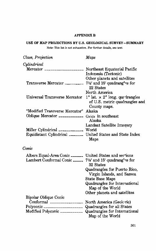
APPENDIXB
USE OF MAP PROJECTIONS BY U.S. GEOLOGICAL SURVEY -SUMMARY Note: This list is not exhaustive. For further details, see text.
Class, Projection Maps
Cylindrical Mercator ------------------- Northeast Equatorial Pacific
Indonesia (Tectonic) Other planets and satellites
Transverse Mercator--------- 7112' and 15' quadrang1a.s for 22 States
North America Universal Transverse Mercator 1° lat. x 2° long. quF1rangles
of U.S. metric quadrangles and County maps.
"Modified Transverse Mercator" Alaska Oblique Mercator------------ Grids in southeast
Alaska Landsat Satellite Ima~ery
Miller Cylindrical ------------ World Equidistant Cylindrical ------- United States and State Index
Maps
Conic
Albers Equal-Area Conic------ United States and seri:ions Lambert Conformal Conic ----- 7112' and 15' quadrang~~s for
32 States
Bipolar Oblique Conic
Quadrangles for Puerto Rico, Virgin Islands, and Samoa
State Base Maps Quadrangles for International
Map of the World Other planets and satellites
Conformal ---------------- North America (Geolcrric) Polyconic ------------------- Quadrangles for all States Modified Polyconic ----------- Quadrangles for International
Map of the World
301
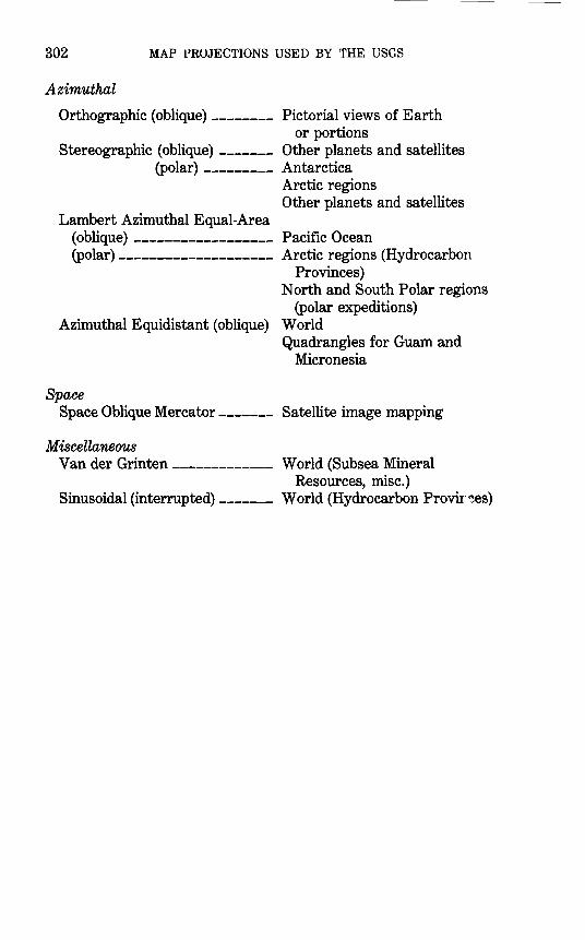
302 MAP PROJECTIONS USED BY THE USGS
Azimuthal
Orthographic (oblique)-------- Pictorial views of Earth or portions
Stereographic (oblique) ------- Other planets and satellites (polar)--------- Antarctica
Arctic regions Other planets and satellites
Lambert Azimuthal Equal-Area (oblique) ------------------ Pacific Ocean (polar) -------------------- Arctic regions (Hydrocarbon
Provinces) North and South Polar regions
(polar expeditions) Azimuthal Equidistant (oblique) World
Space
Quadrangles for Guam and Micronesia
Space Oblique Mercator------- Satellite image mapping
Miscellaneous Van der Grin ten ------------- World (Subsea Mineral
Resources, misc.) Sinusoidal (interrupted) ------- World (Hydrocarbon Provir~es)
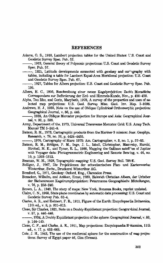
REFERENCES Adams, 0. S., 1918, Lambert projection tables for the United States: CS. Coast and
Geodetic Survey Spec. Pub. 52. --, 1919, General theory of Polyconic projections: U.S. Coast and <*-odetic Survey
Spec. Pub. 57. --, 1921, Latitude developments connected with geodesy and car0graphy with
tables, including a table for Lambert Equal-Area Meridional projection: U.S. Coast and Geodetic Survey Spec. Pub. 67.
--, 1927, Tables for Albers projection: U.S. Coast and Geodetic Surw~y Spec. Pub. 130.
Albers, H. C., 1805, Beschreibung einer neuen Kegelprojektion: Zach's Monatliche Correspondenz zur Beforderung der Erd- und Himmels-Kunde, Nov., p. 450-459.
Alpha, Tau Rho, and Gerin, Marybeth, 1978, A survey of the properties and uses of selected map projections: U.S. Geol. Survey Misc. Geol. lnv. Map. 1-1096.
Andrews, H. J., 1935, Note on the use of Oblique Cylindrical Orthomorphic projection: Geographical Journal, v. 86, p. 446.
--, 1938, An Oblique Mercator projection for Europe and Asia: Georraphical Journal, v. 92, p. 538.
Army, Department of the, 1973, Universal Transverse Mercator Grid: U.S. Army Tech. Manual TM 5-241-8.
Batson, R. M., 1973, Cartographic products from the Mariner 9 mission: .Tour. Geophys. Research, v. 78, no. 20, p. 4424-4435.
--, 1976, Cartography of Mars: 1975: Am. Cartographer, v. 3, no. 1, p. 57-63. Batson, R. M., Bridges, P. M., Inge, J. L., Isbell, Christopher, Masnt'Sky, Harold,
Strobell, M. E., and Tyner, R. L., 1980, Mapping the Galilean satell~~es of Jupiter with Voyager data: Photogrammetric Engineering and Remote Sene-ing, v. 46, no. 10, p. 1303-1312.
Beaman, W. M., 1928, Topographic mapping: U.S. Geol. Survey Bull. 788-E. Bolliger, J., 1967, Die Projektionen der schweizerischen Plan- und Kartenwerke:
Winterthur, Switz., Druckerei Winterthur AG. Bomford, G., 1971, Geodesy: Oxford, Eng., Clarendon Press. Bonacker, Wilhelm, and Anliker, Ernst, 1930, Heinrich Christian Albers, der Urheber
der flachentreuen Kegelrumpfprojektion: Petermanns GeographischE: Mitteilungen, v. 76, p. 238-240.
Brown, L.A., 1949, The story of maps: New York, Bonanza Books, reprint undated. Claire, C. N., 1968, State plane coordinates by automatic data processing: U.S. Coast and
Geodetic Survey Pub. 62-4. Clarke, A. R., and Helmert, F. R., 1911, Figure of the Earth: Encyclopaedia Britannica,
11th ed., v. 8, p. 801-813. Close, Sir Charles, 1921, Note on a Doubly-Equidistant projection: Geogra..,hical Journal,
v. 57, p. 446-448. --, 1934, A Doubly Equidistant projection of the sphere: Geographical Journal, v. 83,
p. 144-145. Close, C. F., and Clarke, A. R., 1911, Map projections: Encyclopaedia B:'itannica, 11th
ed., v. 17, p. 653-663. Cole, J. H., 1943, The use of the conformal sphere for the construction of map projec
tions: Survey of Egypt paper 46, Giza (Orman).
303
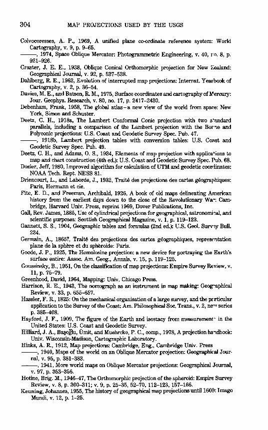
304 MAP PROJECTIONS USED BY THE USGS
Colvocoresses, A. P., 1969, A unified plane co-ordinate reference system: World Cartography, v. 9, p. 9-65.
--, 1974, Space Oblique Mercator: Photogrammetric Engineering, v. 40, ro. 8, p. 921-926.
Craster, J. E. E., 1938, Oblique Conical Orthomorphic projection for New Zealand: Geographical Journal, v. 92, p. 537-538.
Dahlberg, R. E., 1962, Evolution of interrupted map projections: lnternat. Yearbook of Cartography, v. 2, p. 36-54.
Davies, M. E., and Batson, R. M., 1975, Surface coordinates and cartography of Mercury: Jour. Geophys. Research, v. 80, no. 17, p. 2417-2430.
Debenham, Frank, 1958, The global atlas-a new view of the world from space: New York, Simon and Schuster.
Deetz, C. H., 1918a, The Lambert Conformal Conic projection with two s~andard parallels, including a comparison of the Lambert projection with the Bor'le and Polyconic projections: U.S. Coast and Geodetic Survey Spec. Pub. 4 7.
--, 1918b, Lambert projection tables with conversion tables: U.S. CoRSt and Geodetic Survey Spec. Pub. 49.
Deetz, C. H., and Adams, 0. S., 1934, Elements of map projection with applica~ons to map and chart construction (4th ed.): U.S. Coast and Geodetic Survey Spec. Pub. 68.
Dozier, Jeff, 1980, Improved algorithm for calculation of UTM and geodetic coordinates: NOAA Tech. Rept. NESS 81.
Driencourt, L., and Laborde, J., 1932, Traite des projections des cartes geographiques: Paris, Hermann et cie.
Fite, E. D., and Freeman, Archibald, 1926, A book of old maps delineating American history from the earliest days down to the close of the Revolutionary Wa-: Cambridge, Harvard Univ. Press, reprint 1969, Dover Publications, Inc.
Gall, Rev. James, 1885, Use of cylindrical projections for geographical, astronomi"'al, and scientific purposes: Scottish Geographical Magazine, v. 1, p. 119-123.
Gannett, S. S., 1904, Geographic tables and formulas (2nd ed.): U.S. Geol. Surv1y Bull. 234.
Germain, A., 1865?, Traite des projections des cartes geographiques, repreSf'ntation plane de la sphere et du spheroide: Paris.
Goode, J.P., 1925, The Homolosine projection: a new device for portraying the Earth's surface entire: Assoc. Am. Geog., Annals, v. 15, p. 119-125.
Goussinsky, B., 1951, On the classification of map projections: Empire Survey Review, v. 11, p. 75-79.
Greenhood, David, 1964, Mapping: Univ. Chicago Press. Harrison, R. E., 1943, The nomograph as an instrument in map making: Geog":"aphical
Review, v. 33, p. 655-657. Hassler, F. R., 1825: On the mechanical organisation of a large survey, and the pfrticular
application to the Survey of the Coast: Am. Philosophical Soc. Trans., v. 2, ne'H series p. 385-408.
Hayford, J. F., 1909, The figure of the Earth and isostacy from measurement:> in the United States: U.S. Coast and Geodetic Survey.
Hilliard, J. A., B~oglu, Umit, and Muehrcke, P. C., comp., 1978, A projection ha"ldbook: Univ. Wisconsin-Madison, Cartographic Laboratory.
Hinks, A. R., 1912, Map projections: Cambridge, Eng., Cambridge Univ. Press. --, 1940, Maps of the world on an Oblique Mercator projection: GeographiC'.al Jour-
nal, v. 95, p. 381-383. . --, 1941, More world maps on Oblique Mercator projections: Geographical Journal,
v. 97, p. 353-356. Hotine, Brig. M., 1946-47, The Orthomorphic projection of the spheroid: Empire. Survey
Review,v. 8,p. 300-311;v.9,p.25-35, 52-70,112-123,157-166. Keuning, Johannes, 1955, The history of geographical map projections until1600: Imago
Mundi, v. 12, p. 1-25.
REFERENCES 305
Laborde, Chef d'escadron, 1928, La nouvelle projection du service gtographique de Madagascar: Cahiers due Service geographique de Madagascar, Tananarive, no. 1.
Lallemand, Ch., 1911, Sur les deformations resultant du mode de con,truction de la Carte internationale du monde au millionieme: Comptes Rendus, v. 153, p. 559-567.
Lambert, J. H., 1772, Beitrage zum Gebrauche der Mathematik und der£.n Anwendung: Part III, section 6: Anmerkungen und Zusatze zur Entwerfung der Land- und Himmelscharten: Berlin. Translated and introduced by W. R. Tobler, r1iv. Michigan, 1972.
Lee, L. P., 1944, The nomenclature and classification of map projections: Empire Survey Review, v. 7, p. 190-200.
--, 1976, Conformal projections based on elliptic functions: Cartographica, Monograph 16.
Lewis, Brig. Sir C., and Campbell, Col. J. D., ed., 1951, The American Oxford atlas: New York, Oxford Univ. Press.
Maling, D. H., 1960, A review of some Russian map projections: Empire f''ll'Vey Review, v. 15,no. 115,p. 203-215;no. 116,p. 255-266;no. 117,p.294-303.
--, 1973, Coordinate systems and map projections: London, Geor~ Philip & Son, Ltd.
Maurer, Hans, 1919; Annalen der Hydrographie, p. 77. --, 1935, Ebene Kugelbilder: Gotha, Germany, Petermanns Geographische
Mitteilungen, Erg8nzungsheft 221. Translated with editing and foreword by William Warntz, Harvard papers in theoretical geography, 1968.
McDonnell, P. W., Jr., 1979, Introduction to map projections: New York, J lfarcel Dekker, Inc.
Miller, 0. M., 1941, A conformal map projection for the Americas: Geogrz,phical Review, v. 31, p. 100-104.
--, 1942, Notes on cylindrical world map projections: Geographical Review, v. 32, p. 424-430.
--, 1953, A new conformal projection for Europe and Asia [sic; should read Mrica]: Geographical Review, v. 43, p. 405-409.
Mitchell, H. C., and Simmons, L. G., 1945, The State coordinate systems (a manual for surveyors): U.S. Coast and Geodetic Survey Spec. Pub. 235.
National Academy of Sciences, 1971, North American datum: National Ocean Survey contract rept. E-53-69(N), 80 p., 7 figs.
Nordenskiold, A. E., 1889, Facsimile-atlas: New York, Dover Publication"~ Inc., (reprint 1973).
O'Keefe, J. A., and Greenberg, Allen, 1977, A note on the Vander Grinocn projection of the whole Earth onto a circular disk; Am. Cartographer, v. 4, no. 2, p. 127-132.
Pearson, Frederick II, 1977, Map projection equations: Dahlgren, Va., Naval Surface Weapons Center.
Pettengill, G. H., Campbell, D. B., and Masursky, Harold, 1980. The surface of Venus: Scientific American, v. 243, no. 2, p. 54-65.
Rahman, G. M., 1974, Map projection: Karachi, Oxford Univ. Press. Raisz, Erwin, 1962, Principles of cartography: New York, McGraw-Hill. Richardus, Peter, and Adler, R. K., 1972, Map projections for geodesists, cartographers,
and geographers: Amsterdam, North-Holland Pub. Co. Robinson, A. H., Sale, R. D., and Morrison, J. L., 1978, Elements of ca"i;ography (4th
ed.): New York, John Wiley and Sons. Rosenmund, M., 1903, Die Anderung des Projektionssystems der s~~hweizerischen
Landesvermessung: Bern, Switz. Royal Society, 1966, Glossary of technical terms in cartography: Appendix 1: Named map
projections: London, The Royal Society. Rubincam, D. P., 1981, Latitude and longitude from Van der Grinten grid coordinates:
Am. Cartographer, v. 8, no. 2, p. 177-180.
306 MAP PROJECTIONS USED BY THE USGS
Snyder, J. P., 1977, A comparison of pseudocylindrical map projections: .Am. Cartographer, .v. 4, no. 1, p. 59-81.
--, 1978a, Equidistant Conic map projections: Assoc. Am. Geographers, Annals, v. 68, no. 3,p. 373-383.
__ , 1978b, The Space Oblique Mercator projection: Photogrammetric Enpneering and Remote Sensing, v. 44, no. 5, p. 585-596.
--, 1979a, Calculating map projections for the ellipsoid: Am. Cartographer, v. 6, no. 1, p. 67-76.
--, 1979b, Projection.notes: Am. Cartographer, v. 6, no. 1, p. 81. --, 1981, Space Oblique Mercator projection-mathematical developm?.nt: U.S.
Geol. Survey Bull. 1518. --, 1981a, Map projections for satellite tracking: Photogrammetric Engine~ring and
Remote Sensing, v. 47, no. 2, p. 205-213. Steers, J. A., 1970, An introduction to the study of map projections (15th ed.): London,
Univ. London Press. Thomas, P. D., 1952, Conformal projections in geodesy and cartography: U.S. Coast and
Geodetic Survey Spec. Pub. 251. --, 1970, Spheroidal geodesics, reference systems, and local geometry: U.S. Naval
Oceanographic Office. Thompson, M. M., 1979, Maps for America: U.S. Geol. Survey. Tissot, A., 1881, Memoire sur Ia representation des surfaces et les projections d~s cartes
geographiques: Paris, Gauthier Villars. Tobler, W. R., 1962, A classification of map projections: Assoc. Am. Georraphers,
Annals, v. 52, p. 167-175. See also refs. in Maling (1973, p. 98-104) and Maurer (1935, as translated 1968, p. v-vii).
U.S. Coast and Geodetic Survey, 1882, Report of the Superintendent of the U.S. Coast and Geodetic Survey * * * June 1880: Appendix 15: A comparison of th~ relative value of the Polyconic projection used on the Coast and Geodetic Survey, "'·ith some other projections, by C. A. Schott.
--, 1900, Tables for a Polyconic projection of maps: U.S. Coast and Geodeti'c Survey Spec. Pub. 5.
U.S. Geological Survey, 1964, Topographic instructions of the United States Geological Survey, Book 5, Part 5B, Cartographic tables: U.S. Geol. Survey.
--, 1970, National Atlas of the United States: U.S. Geol. Survey. United Nations, 1963, Specifications of the International Map of the Wor1d on the
Millionth Scale, v. 2: New York, United Nations. Vander Grinten, A. J., 1904, Darstellung der ganzen Erdoberflache auf einer Kreisfor
migen Projektionsebene: Petermanns Geographische Mitteilungen, v. 50, p.155-159. --, 1905, Zur Verebnung der ganzen Erdoberflache. Nachtrag zu der Dars~ellung in
Pet. Mitt. 1904 * * *: Petermanns Geographische Mitteilungen, v. 51, p. 2:'7. VanZandt, F. K., 1976, Boundaries of the United States and the several Str.tes: U.S.
Geol. Survey Prof. Paper 909. World Geodetic System Committee, 1974, The Department of Defense World Geodetic
System 1972. Presented by T. 0. Seppelin at the lnternat. Symposium on Problems Related to the Redefinition of North American Geodetic Networks, Frt'dericton, N.B., Canada, May 20-25, 1974.
Wraight, A. J., and Roberts, E. B., 1957, The Coast and Geodetic Survey, 1f07-1957: 150 years of history: U.S. Coast and Geodetic Survey.
Wray, Thomas, 1974, The seven aspects of a general map projection: Cartcgraphica, Monograph 11.
Young, A. E., 1930, Conformal map projections: Geographical Jour., v. 76, no. 4, p. 348-351.
INDEX
[Italic page numbers indicate mlijor references]
A
Page
Acronyms --------------------------XIII Adams, 0. S ________________ 2, 17, 18, 93, 95
Aeronautical chwrts ------------------104 ADica, mapsof _________________ l56,219
Alaska, maps oL_3, 56, 69, 73, 76, 81, 95, 301 Albers, H. C --------------------------93 Albers Equal-Area Conic projection _31, 99-99,
101, 103 feanues _______________________ 93-95
formulas, ellipsoid _______ 96-99, 245-248 sphere ___________ 95-96,99,243-245
histo~---------------------------93 polar coordinates __________________ 99 usage ___________ 3,92,93-95,128,301
American Geographical Society __ 85, 111, 114, 158
American Polyconic projection __________ 123 American Telephone & Telegraph Co _____ 180 Analemma projection ________________ 141 Antarctica, maps of ______________ 3, 156, 302
Aposphere -------------------------7 4, 78 Arab cartographers __________________ 153 ArctanfUnction,general ________________ XII Arctic regions, maps of _________ 158, 170, 302 Army Map Service ---------------------63 Astrogeology, USGS Center of _______ 47, 158 ATAN2 fUnction, Fortran, general _______ XII Atlantic Ocean, maps of ________________ 51
Authalic latitude See latitude, authalic
Authalic projections -------------------6 Auxiliary latitudes
See latitudes, auxilia~ Azimuth, calculation ___________________ 34
symbols _________________________ XI
Azimuthal Equal-Area projection ________ 167 Azimuthal Equidistant projection ___ 9,179-192
features _____________ l36,180-182,183
formulas, ellipsoid _185, 187-192, 275-281 sphere ____________ l84-185,273-275
geometric construction _______ 182, 184
histo~------------------179-180 polar coordinates _____________ 139, 187 rectangular coordinates _____________ 186 usage ____________________ l82,302
Page
Azimuthal projections_6, 8, 9, 3r, 135-139,302 scale and distortion ____________ 25, 30, 31 transformation ______________ 33-38 See also Azimuthal Equidist->nt projection,
Lambert Azimuths 1 Equal-Area projection, Orthograrhic projection, Stereographic projertion
B
Basement Map --------------------113 Bathymetric Map ----------------------45 Bipolar Oblique Conic Conf1rrnal projec-
tion --------------------111, 119-121
feanues and usage __ 56, 11f-114, 119,301 formulas, sphere _____ 11o:t-118, 252-254 histo~ ______________ 2,85,111,113 rectangular coordinates _________ 120-121
Bo~,s.vv ________________________ 85,87 Bomford, G _________________________ l80 Borneo, mapsof ___________________ 73, 76 Briesemeister, VV. A ______________ 111, 113
c Cagnoli, A ------------------------180 Calculator,pocket ______________ 2,7,33,74 Carte Parallelogrammatique, La __________ 89
Cassini-Soldner projection ---------------63 Chamberlin, VV -----------------------180 Chamberlin Trimetric projection _________ 180 Clarke, A. R ---------------------------16 Clarke 1866 ellipsoid ________________ 15, 209
corrections for auxilia~ latit1tdes using _22 dimensions ________________ 15, 16 distortion of sphere vs ______________ 31 formulas using ____________ 18, 19, 20, 21 length of degree using ______________ 29 use, Guam projection _____________ 188
maps of U.S. ___________ 95, 99, 112 Mercator projection tables ________ 52 Micronesia mapping _____________ 190 Polyconic projection tabk~s _____ 126,
131-133 State Plane Coordinate System ___ 56 Universal Transverse Mercator
projection _______________ 64,71
307
308 MAP PROJECTIONS USED BY THE USGS
Page
"Clarke's best formula" _____________ 189, 191 Classification of projections ___________ 39-40
Close, C. F ---------------------------180 Cole, J. H -----------------------74, 76, 79 Colvocoresses, A. P ___________________ 194 Computer ______________________ 2,7,33,74 Cone, basis of projection ___________ 7, 8, 9, 91 Coneconstantn ___ XI, 25, 92, 96, 105,107,114 Conformal latitude
See latitude, conformal Conformal projections _2, 6, 7, 19, 23, 26-27, 39
See also Bipolar Oblique Conic Conformal projection, Lambert Conformal Conic projection, Mercator projection, Oblique Mercator projection, Space Oblique Mercator projection, Stereographic projection, Transverse Mercator projection
Conic (conical) projections _7, 9, 39, 91-92, 301 scale and distortion _________ 24, 25, 30, 31 transformation _____________________ 33
See also Albers Equal-Area Conic pro-jection, Bipolar Oblique Conic Conformal projection, Lambert Conformal Conic projection, Polyconic projection
Conical Orthomorphic projection _________ 101 Conrad of Dyffenbach _________________ 179 Convergence of meridians ___________ 24-25
Coordinates, polar --------------------25 rectangular ____________________ XI, 25
See also specific projection Cossin, J ----------------------------219 Curvature,radiusof ____________ 28,228-229
total __________________________ 7 4, 78
Cylinder, basis of projection __________ 7, 8, 9 Cylindrical Equal-Area projection ______ 41, 94 Cylindrical projections _______ 7, 9, 39, 41, 301
scale and distortion _________ 24, 25, 29, 31 transformation _________________ 33-38
See also Cylindrical Equal-Area projection, Equidistant Cylindrical projection, Mercator projection, Miller Cylindrical projection, Oblique Mercator projection, Simple Cylindrical projection, Transverse Equidistant Cylindrical projection, Transverse Mercator projection
D d'Aiguillion, F ___________________ 141, 153
Datum --------------------------13-16 Debenharn, F ---------------------144 Deetz, C. H --------------------------2 Defense Mapping Agency ______________ 16 Deformation, maximum angular _23, 24, 27, 96,
103, 202, 210 De Lorgna --------------------------167 Distortion of maps
See deformation, maximum angular; scale
Page
Donald, J. K --------------------------180 DUrer, A ----------------------------141
E Easting, false ________________________ XI
Egyptian cartographers ________ 141. 153, 179 Ellipsoid, Earth taken as _____________ 13-16
eccentricity, symbols ____________ XI, 16 flattening ___________________ 13, 15, 16 Scale and distortion _____________ 28-31
Stereographic projection charactE'~'-istics ______________________ 156
See also Clarke 1866 ellipsoid; International ellipsoid; Latitude, auxiliary; specific projection
Equal-area projections __________ 5-6, 19, 39 See also Albers Equal-Area Con;<'! projec
tion, Cylindrical Equal-Ar~a projection, Lambert Azimuthal EqualArea projection, Sinusoid'1'1 projection
Equatorial projections _________ 9, 3l, 36, 135 Azimuthal Equidistant _____________ 181 Lambert Azimuthal Equal-Area _____ 168 Orthographic ________________ 142, 143 Stereographic ___________________ 154
Equiarealprojections ___________________ 6
Equidistant Conic projection _______ 69, 71, 91 Equidistant Cylindrical projection ___ 89-90, 92,
222,301 formulas, for sphere _______________ 90 history and features __________ 89-90
Equidistant projections _______________ 6, 39 See also Azimuthal Equidistant rrojection,
Equidistant Conic pr"~jection, Equidistant Cylindrical projection
Equirectangular projection ______________ 89
Equivalent projections -----------------6 Eratosthenes ____________________ 89
ERT8-1 -----------------------193 Etzlaub, E ------------------------43 Europe, map of -----------------------156 Extraterrestrial mapping ___________ 3, 17
Lambert Conformal Conic projectfon __ 106, 301
Mercator projection _______ 48-4'\ 51, 301 Stereographic projection, oblique _156, 302
polar --------------------157, 302 Transverse Mercator projection _______ 63
F
Flamsteed, J ---------------------219 Fourierseries ____________ l98, 200,206,209
G Galilean satellites of Jupiter
See Jupiter satellites
INDEX 309
Page Gall,J ________________________________ 85
Gall's Cylindrical projection ________ 41, 85, 87
Gauss, C. F ---------------------------53 Gauss conformal projection ______________ 54 Gauss-Kruger projection ________________ 54 Geodetic Reference System ___________ 15, 16
Ge~pkia ---------------------------89 Geologic maps __________________ 56, 93,301
Geothermal Map ----------------------113 Germain, A ---------------------------54 Ginsburg, G. A -----------------------167 Glareanus ---------------------------180 Globular projection ________________ 170, 181 Gnomonic projection _________ 6, 135, 138, 180
Goode, J. P --------------------------221 Goode's Atlas -------------------------221 Great circle distance ________________ 34, 146 Great circle paths _____________ 6, 34, 45, 135
Greenwich meridian --------------------11 Grid declination ---------------------·---24 Guam projection __ 182, 188, 191, 276, 279, 302
H
Harrison, R. E ------------------------144 Hassler, F. R ___________________ 2, 123, 124
Hatt, P ------------------------------180 Hawaii,mapsof __________________ 45,76,95
Hayford, J. F --------------------------13 Hayford ellipsoid -----------------------15 Heat Capacity Mapping Mission (HCMM)
imagery ____________________ 76
Hipparchus _______________ 12, 141, 153, 219 Homalographic projections _______________ 6 Homolographic projections ___________ 6, 221 Homolosine projection _________________ 221
Hondius, J ---------------------------219 Horizon aspect of projections, defi-
nition __________________ 33, 135
Hotine, M ______________ 73, 74, 76, 78, 79, 81 Hotine Oblique Mercator (HOM) projection
See Oblique Mercator projection: Hotine Hydrocarbon Provinces, map of __ 170, 221, 302
I
Ibn-el-Zarkali ------------------------153 Index maps, topographic ____________ 90, 301 Indicatrix, Tissot's ___________ ..29-25, 31, 195 Indonesia, maps of _________________ 47, 301 International ellipsoid ___________________ 56
dimensions _____________________ 13, 15 length of degree using _______________ 29 use with polar projections ___ 164, 165, 177,
187 use in Universal Transverse Mercator
projection ___________________ 64
Page
International Map Committee ___________ 133 International Map of the World (IMW) ____ 104,
l3R-134, 156, 301 International Union of Geodesy and
Geophysics (IUGG) ________ 13, 16 Inverse equations, for auxiliary latitudes ____ _
18-21 for projections
See specifw projection for transformations _____________ 35, 36
Isometric latitude ___________ 18-19, 226-227
Italy, map of --------------------------76
J
Junkins, J. L -------------------------194 Jupiter satellites, maps of
Lambert Conformal Conic projection ______________ 104,106
Mercator projection ______________ 47, 49 reference spheres ________________ 16, 17 Stereographic projection ________ 157, 158
K
Kavraisky, V. V -----------------------95 Kepler's laws -------------------------203 Kruger, L ----------------------------53
L
Laborde, J. --------------------73,76,79 Lallemand,C _________________________ 133
Lambert, J. H ______________ 53, 54, 101, 167 Lambert Azimuthal Equal-Area projection __ 3,
94, 135, 1~~, 167-177, 302 coordinates, polar __________________ 177
rectangular ________________ 174, 175 features ______________________ 167-169
formulas, ellipsoid _____ 173-177, 269-273 sphere ________ 170,172-173,267-269
geometric construction _____________ 170
history ------------------------53, 167 usage ________________________ 170, 181
Lambert Conformal Conic proj~ction _101-109, 113
features ___________________ 26, 101-103
formulas, ellipsoid _____ 107-109, 250-252 sphere ____________ 10i, 107,248-250
history ________________________ 53, 101 polar coordinates __________________ 112 usage ___________ 3,92,10~-104,128,301
in extraterrestrial mapping ______ 106 in International Map of the
World _________________ 134, 156
in State Plane Coordina~P. System ___ 3, 56,58,60-62,103,127
310 MAP PROJECTIONS USED BY THE USGS
Page
Lambert's Cylindrical Equal-Area projection ______________ 4l, 94
Lambert's Equal-Area Conic projection ____ 94 Landsat imagery, Hotine Oblique Mercator
projection ____ 76, 77,194, 195,301 Space Oblique Mercator projection ___ 193,
194,195,198,203,209-210,302 Latitude, authalic _____ 19-20, 22, 98, 173, 176,
227-228 auxiliary _______________ 16-22, 225-228
See also latitude: Authalic, conformal, geocentric, isometric, parametric, reduced
conformal_17,18-19,22,74, 108,160,163, 225-226
footpoint --------------------------68 geocentric ____ 16-17,21,22, 108,109,228 geodetic _______ XII, 7, 9, 11-12, 14, 16, 17
length of degrees _____________ 28, 29 scale and distortion ___________ 24, 25 standard
See parallels, standard See also specific projection
geographic See latitude, geodetic
isometric _______________ 18-19, 226-227 parametric or reduced _______ _21, 22, 228 "pseudotransformed" _______________ 203 ~ng __________ J0-21,22,188,228 reduced or parametric _______ _21, 22, 228 transformed __ xu, 33, 35, 67, 74, 113, 199
Lee, L. P ----------------------------_55 Longitude
geodetic _____________ XII, 7, 9, 11-12, 14 length of degree ______________ 28, 29 scale and distortion ___________ 24, 25 See also specific projection
"pseudotransformed" _______________ 203 "satellite-apparent" ______________ 199 transformed __ XII, 33, 35, 67, 74, 113, 199
Loritus, H -------------------------180 Loxodromes _____________________ 43, 45
Ludd,VV ---------------------------153
M
Madagascar, maps of ______________ 73, 76
Malaya, maps of -----------------------76 Map projections -----------1-40, 301-302
See also specific projection
Maps for America -----------------------2 Marinus of Tyre ------------------------89 Mars, maps of -------------------------3
Lambert Conformal Conic projection ______________ 104, 106
Mercator projection _____________ 47, 48 reference ellipsoid ______________ 16, 17
Page
Mars, maps of- Continued Stereographic projection ____ 156, 157, 158 Transverse Mercator projection ______ 63
Maurer, H ________________________ 40, 180
Meades Ranch, Kans ____________________ 15 Mercator, G ________________ 43, 44, 180, 219
Mercator, R --------------------------153 Mercator Equal-Area projection _________ 219 Mercatorprojection ___ 7, 41,49-52,74,87, 101
features ______________________ 6,45,46
formulas, ellipsoid _18, 19, 50-51, 230-231 sphere __________________ 47,49,229
history _________________________ 43-45
Oblique See Oblique Mercator projection
rectangular coordinates _____________ 52
Transverse See Transverse Mercator proj£~tion
usage ______________________ 4f,47,301
in extraterrestrial mapping __ .;l8-49, 51 with another standard parallel _________ 51
Mercury, maps of ----------------------3 Lambert Conformal Conic
projection ______________ 104,106
Mercator projection ------------4 7, 48 reference sphere ________________ 16, 17 Stereographic projection ___ 156, 157, 158 Transverse Mercator projection ______ 63
Meridian central _______________ xn, 12, 55, 58-60
See also specific projection prime ____________________________ 11
Meridian aspect of projection ________ 33, 135
Meridians See longitude
Meridional aspect of projection _______ 33, 135
Metallogenic Map ---------------------113 Metric conversion ----------------------56 Micronesia, mapping of ___ 182, 188, 189, 190,
191,277,280,302 Miller, 0. M ___________ 85, 87, 111, 113, 156 Miller Cylindrical projection ___________ 85-88
features _______________________ 85-87
formulas, sphere _________ 87-88 242-243 history _________________________ 85,87 rectangular coordinates ____________ 88 use _________________________ 2,87,301
Mineral Resources, maps of _________ 211, 302 Modified Polyconic projection ___ 104, 199-194,
156,301 "Modified Transverse Mercator" proje~tion _69,
71-7f! .. 92, 301 Mollweide projection _______________ 213, 221
Moon, maps of Earth's ------------------3 Lambert Azimuthal Equal-Area
projection _________________ 170
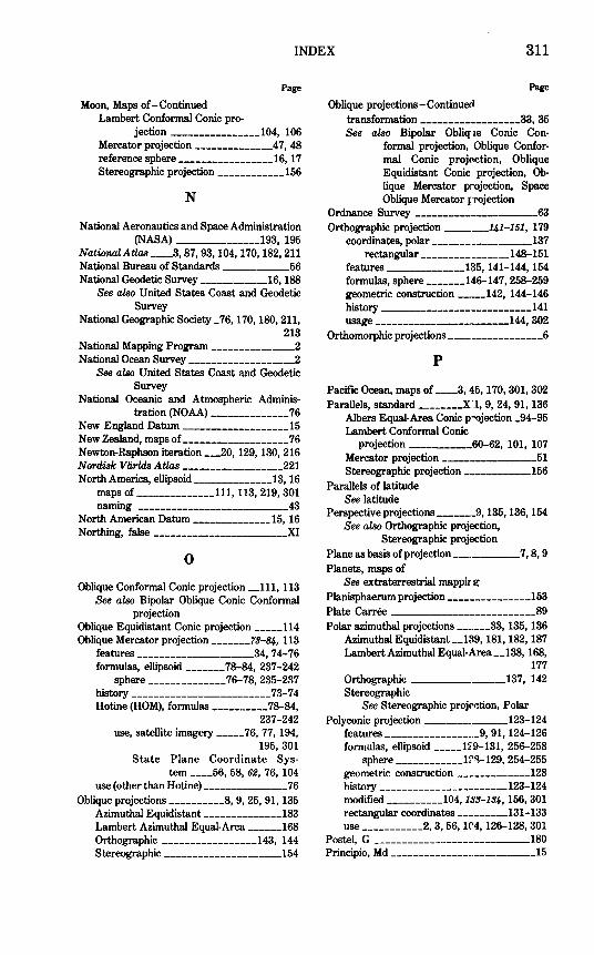
INDEX 311
Moon, Maps of-Continued Lambert Conformal Conic pro-
Page
jection ________________ 104, 106 Mercator projection ______________ 47, 48 reference sphere _________________ 16, 17 Stereographic projection ____________ 156
N
National Aeronautics and Space Administration (NASA) _______________ 193, 195
National Atlas ____ 8, 87, 93, 104, 170, 182, 211 National Bureau of Standards ____________ 56 National Geodetic Survey ____________ 16, 188
See also United States Coast and Geodetic Survey
National Geographic Society _76, 170, 180, 211, 213
National Mapping Program ---------------2 National Ocean Survey -------------------2
See also United States Coast and Geodetic Survey
National Oceanic and Atmospheric Adminis-tration (NOAA) --------------76
New England Datum ___________________ 15 New Zealand, maps of ___________________ 76 Newton-Raphson iteration ___ 20, 129, 130, 216 Nrmiisk Viirlds Atlas __________________ 221 North America, ellipsoid ______________ 13, 16
maps of ______________ 111, 113, 219, 301
naming ---------------------------43 North American Datum ______________ 15, 16 Northing, false ________________________ XI
0
Oblique Conformal Conic projection __ 111, 113 See also Bipolar Oblique Conic Conformal
projection Oblique Equidistant Conic projection _____ 114 Oblique Mercator projection _______ 79-81,, 113
features _____________________ 34,74-76
formulas, ellipsoid _______ 78-84, 237-242 sphere ______________ 76-78, 235-237
history -------------------------73-7 4 Hotine (HOM), formulas ----------78-84,
237-242 use, satellite imagery _____ 76, 77, 194,
195, 301 State Plane Coordinate Sys-
tem ____ 56, 58,62, 76,104 use(otherthanHotine) _______________ 76
Oblique projections __________ 8, 9, 25, 91, 135 Azimuthal Equidistant ______________ 183 Lambert Azimuthal Equal-Area ______ 168 Orthographic _________________ 143, 144 Stereographic _____________________ 154
Page
Oblique projections-Continue<\ transformation __________________ 33, 35 See also Bipolar Oblique Conic Con
formal projection, Oblique Conformal Conic projElction, Oblique Equidistant Conic projection, Oblique Mercator projection, Space Oblique Mercator rrojection
Ordnance Survey ----------------------63 Orthographic projection ________ 11,1-151, 179
coordinates,polar __________________ 137 rectangular ________________ 148-151
features ______________ l35,141-144,154 formulas, sphere _______ 146-147, 258-259 geometric construction _____ 142, 144-146 history ___________________________ 141 usage ________________________ l44,302
Orthomorphic projections -----------------6
p
Pacific Ocean, maps of ____ 3, 45, 170, 301, 302 Parallels, standard ________ X~I, 9, 24, 91, 136
Albers Equal-Area Conic p~ojection _94-95 Lambert Conformal Conic
projection ___________ 60-62, 101, 107 Mercator projection _________________ 51 Stereographic projection __________ 156
Parallels of latitude See latitude
Perspective projections _______ 9, 135, 136, 154 See also Orthographic projection,
Stereographic projection Plane as basis of projection ____________ 7, 8, 9
Planets, maps of See extraterrestrial mappire;
Planisphaerum projection _______________ 153
Plate Carree --------------------------89 Polar azimuthal projections ______ 33, 135, 136
Azimuthal Equidistant __ 139, 181, 182, 187 Lambert Azimuthal Equal-Area __ 138, 168,
177 Orthographic _________________ 137, 142
Stereographic See Stereographic proj('ction, Polar
Polyconic projection _______________ 123-124 features _________________ 9,91,124-126 formulas, ellipsoid _____ 129-131, 256-258
sphere ____________ lr~129, 254-255 geometric construction _____________ 128 history _______________________ 123-124 modified __________ 104, 199-191,, 156, 301 rectangular coordinates _________ 131-133 use ___________ 2,3,56,1r4, 126-128,301
Postel, G ----------------------------180 Principio, Md --------------------------15
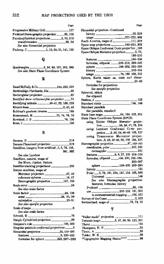
312 MAP PROJECTIONS USED BY THE USGS
Page
Progressive Military Grid _______________ 127 Prolated Stereographic projecti~n _____ 85, 156 Pseudocylindrical projections _______ 9, 39, 219
transformation __________________ 33, 34
See also Sinusoidal projection Ptolemy, C ____________ 1, 12, 89, 91, 141, 153
Q
~rangles _________ 3, 56, 63,157,301,302 See also State Plane Coordinate System
R
Rand McNally & Co ____________ 144, 219, 221 Rechteckige Plattkarte, Die ______________ 89 Rectangular projection __________________ 89 Rectified skew orthomorphic projection ____ 73 Rec~glatitude _______ _2Q-21,22, 188,228
Rhumb lines ----------------------6, 43, 45 Robbins's geodesic inverse ---------~----189 Rosenmund, M _______________ 73, 7 4, 76, 79 Rowland, J. B _____________________ 76, 195
Roze, J -----------------------------153
s Sanson, N ---------------------------219 Sanson-Flamsteed projection ____________ 219 Satellites, imagery from artificial_3, 6, 76, 193,
See also Landsat Satellites, natural, maps of
See Moon, Jupiter, Saturn
301, 302
Satellite-tracking projections ____________ 193
Saturn satellites, maps of Mercator projection ______________ 47, 49 reference spheres ________________ 16, 17 Stereographic projection ________ 157, 158
Scale error --------------------------24 See also scale factor
Scale factor -----------------------24, 136 areal -----------------------28, 30, 50 calculation _____________________ 23-31
See also specijw projection Scale of maps ---------------------------6
See also scale factor
Schmid, E ----------------------------76 Simple Cylindrical projection _____________ 89 Simpson's rule ____________________ 199, 282 Singular points in conformal projections _____ 6 Sinusoidal projection ____________ 34, 219-222
features ____________________ 9,220-222
formulas for sphere _______ 222, 297-298
Page
Sinusoidal projection-Continued h~tory ________________________ 53,219
usage ____________________ 221 ~222, 302 South America, maps of ____________ 111, 219 Space map projections _________ 193-210, 302 Space Oblique Conformal Conic projec~on _193 Space Oblique Mercator projection ______ 3, 79,
193-210 features ----------------------194-198 formulas, ellipsoid _____ 203-210, 289-295 sphere _______________ 198-202, 281-289 ~tory _______________________ 193-194 usage _________________ 76, 195,. 198, 302
Sphere, Earth taken as, scale an1 d~tor-tion _____________________ 25-28
formulas for projections See specific pro}ection
Spheroid, oblate See ellipsoid
Stabius, J ---------------------------153 Standard circle ___________________ 156, 160
Standard parallels See parallels, standard
State base maps ___________ 64, 104, 128, 301 State Plane Coordinate System (SPCS)
using Hotine Oblique Mercato:w projec-tion ___________ 56, 58, 6.'?, 76, 104
using Lambert Conformal Cc nic pro-jection ___ 3, 56, 58, 60-62. 103, 127
using Transverse Mercator projection _3, 56, 58-60, 68, 103 104, 127
Stereographic projection _________ 6'1, 158-16/'i
coordinates, polar ---~----------137, 165 rectangular ____________________ 161
features ___________ 6,9,27,135 154-156 formulas, ellipsoid _____ 156, 160, 162-164,
260-267 sphere ____________ 158-160.259-260
history ___________________________ 153
Polar ___ 3, 79, 101, 134, 137, 154. 165, 302 Universal ---------------------156 See also Stereographic p·ojection: features; formulas; history
Prolated ----------------------85, 156 use __________________ 156-158 181,302
in extraterrestrial mapping ___ 156, 157 Survey of the Coast __________________ 2, 123 Switzerland, maps of _____________ 73, 74, 76
T
"Tailor-made" projection _______________ 111 Tectonic maps _________ 3, 47, 56, 93. 113,301 Theon _______________________________ 153 Thompson, E. H _______________________ 55
Tissot, A -----------------------------23 Tobler, W. R --------------------------39 "Topographic Mapping Status•••" ________ 90
INDEX 313
Page
Topographic maps ----------------------25 See also quadrangles
Transformation of graticules __________ 33-38 See also specific projectioo
Transverse Equidistant Cylindrical projec-
tion ------------------------63 Transverse Mercator projection _17, 33,59-72,
73, 79 features _____________________ 26,55,57
formulas, ellipsoid __ 54, 55, 67-69, 232-235 sphere ______________ 64, 67,231-232
hffitory _______________________ 2,53-55
"Modified" ____________ 69, 71-72, 92, 301 rectangular coordinates ___________ 70, 71 Universal (UTM) _56, 69-61,., 65, 66, 71, 104,
127, 156, 301 use ________________ 55-64, 113,127,301
in State Plane Coordinate System __________________ 3, 56,
58-60,68,103,104,127 Transverse projections ___________ 8, 9, 33, 36
See also Transverse Mercator projection Two-Point Azimuthal projection _________ 180 Two-Point Equidistant projection ________ 180
u United Nations (UN} _______________ 134, 156
United States, maps of ____ 73, 93, 95, 128, 301 United States Coast and Geodetic Survey _2, 3,
13, 76, 93, 103, 123, 130 United States Standard Datum ___________ 15
Universal Polar Stereographic projection __ 156
Page
Universal Transverse Mercator (UTM) projection
See Transverse Mercator projection, Universal
v Van der Grinten, A. J ______________ 211, 213 Vander Grinten projection _________ ..211-218
features ______________________ 211-213
formulas, sphere _______ 214-216, 295-299 geometric construction _____________ 213
history -------------------------2, 211 rectangular coordinates _________ 216-218 use ______________________ 211-213,302
Vaulx,J. de __________________________ 153 Venus, maps of, Mercator proje<'tion ____ 4 7, 48
reference sphere _________________ 16, 17
w Washington, D.C., meridian --------------11
Universal Transverse Mercator (UTM)
zone -----------------------64 Werner, J ---------------------------153 Westlndies,mapsof ____________________ 76
World, maps of _45, 85, 179, 211, 221, 301, 302 World Geodetic System(WGS) ______ 14, 15, 16
W~ht, E ----------------------------45
z Zenithal Equal-Area projection __________ 167 Zenithal projections _________________ 6, 135
Zinger, N. J ---------------------------95
*U.S. GOVERNMENT PRINTING OFFICE : 1983 0 - 408-476 : QL 3


