Kinds of unpredictability in deterministic systems

Kinds of Unpredictability in Deterministic Systems

G. Schurz

Universit/it Salzburg, Austria

1 I n t r o d u c t i o n

Deterministic chaos is often explained in terms of the unpredictability of certain deterministic systems. For the traditional viewpoint of determinism, as expressed in the idea of Laplace (Weingartner (these proceedings), ch. 1.1), this is rather strange: how can a system obey deterministic laws and still be unpredictable? So there is an obvious lession which philosophy of science has to learn from chaos theory: that determinism does not imply predictability. But besides this obvious point, there is much conceptual unclarity in chaos theory. There are several different and nonequivalent concepts of predictability, and accordingly, different concepts of chaos. In this paper I will differentiate several different concepts of predictability. I will discuss their significance and their interrelations and finally, their relation to the concept of chaos. I will focus on very simple examples of graphically displayed trajectories of particles (usually in a one-dimensional space), without going into the mathematical details of the dynamical genera- tion of these trajectories from fundamental equations. I think that all major conceptual problems can already be discussed at hand of these simple examples.

A dynamical system is defined by its state space (or phase space) S. The state space of systems of classical mechanics has to contain, for each particle, its position and its velocity - - or in the Hamiltonian description its position and its momentum - - in the 3-dimensional Euclidean space (cf. Bat terman (1993), p. 46). Classical dynamics is interested in determining the temporal development of such a system from some fundamental equations - - usually differential equations - - describing the forces which act on the particle(s) of that system. The solutions of these differential equations are functions s : T -~ S which describe the possible movements of particles in S in dependence on time and are called (time-dependent) trajectories. In the example of planetary systems, the possible trajectories are either periodic orbits or collapse trajectories where a planet col- lapses into the sun, or escape trajectories where a planet escapes the attraction of the sun. Note that the understanding of notion of trajectory among physicists is not unique: besides the t ime-dependent notion of t rajectory there is also a time-independent notion of t rajectory (cfi fig. 9). 1 In the normal case we under-

I Chirikov understands "trajectory" in a time-dependent sense (Chirikov (these proceedings), ch. 2.1), Batterman in a time-independent sense (Batterman (1993), p. 47)

thphil

Schreibmaschinentext

"Kinds of Unpredicatability in Deterministic Systems", in: P. Weingartner/G. Schurz (Hg.), "Law and Prediction in the Light of Chaos Research", Springer, Berlin 1996, S. 123-141.

124 Gerhard Schurz

stand the t ime t and position s in S to be continuous real-valued parameters; exceptions where a discrete modeling is assumed will be explicitly mentioned.

2 The Concept of Determinism

Usually a mechanical system is called determinist ic if its s ta te S(to) at some arbitrari ly chosen intial t ime to determines its state s(t) for each future t ime point t > to - - this is forward d e t e r m i n i s m - and also, for each past t ime point t < to - - this is backward determinism. Of course, the fundamental equations governing the system do not determine the actual t ra jectory of the particle of the system (assume it is a one-particle system). But if the particle 's s ta te S(to) is given for only one t ime point to, then its entire t ra jectory is determined. In other words, a mechanical system is deterministic if its trajectories never branch, neither forward nor backward in time. 2 For practical purposes, forward determinism is more important . But classical dynamical systems are forward as well as backward deterministic - - something which is obvious from their well-known t ime-reversibi l i ty . If the t ime is assumed to be discrete instead of real-valued, there exists an equivalent incremental definition of a deterministic system re- quiring tha t for any given t ime-point tn, the system's state s(tn) determines the immediate successor s tate s( tn+l) - - forward determinism - - and its immediate predecessor s tate S(tn-1) (backward determinism). By induction on n, this definition implies the earlier one.

A central feature of all these characterizations of a deterministic system is the (implicit) modal or eounterfaetual element which they involve. For the definition of determinism says tha t if the given system is in s ta te So at t ime to, it mus t be in s tate sl at t ime tl > to - - in other words, if s ( t l ) ~ s l were true, then S(to) ~ so would have been true. Also the physicist's ta lk of trajectories is modal talk, since a t ra jectory is a possible movement of the system's particle - - possible relative to the fundamental equations of the underlying theory. Actually a particular system moves along only one trajectory; the other trajectories are movements under possible but non-actual circumstances. When Russell (1953), p. 398 suggested his functional definition of determinism - - a system is deterministic if there exists a func t ion of the mentioned kind s : T --* S specifying the system's s tate in dependence on t ime - - he seemingly tried to escape the modal element in the definition of determinism, but without success: he himself noticed tha t this definition is too weak, because the movement of every particle - - be it deterministic or random movement - - can be described as some function of time, though sometimes a rather complex one. 3 So the definition of a deterministic system has always to contain the modal concept of possible trajectories, where in physics, this notion of possibility is of course not understood

as primitive but as relative to the underlying theory.

and Haken in a more complicated sense (Haken (1983), p. 124). The understanding of trajectory used here coincides with that of Chirikov.

2 This was added as a result of my discussion with Robert Batterman. a Cf. the discussion in Stone (1989), p. 124.

Kinds of Unpredictability in Deterministic Systems 125

How can we empirically test whether a given system is deterministic? As always, via empirical generality - - we have to realize a situation of the same kind more than once. One possibility is tha t the underlying theory describes systems of a given kind A, e.g. two particle gravitational systems, and we are able to prepare several systems xi of kind A in a way tha t they all are in the same state s(xi, to) at t ime to. Then we just have to look whether their future development is the same; if so, we have confirmed the hypothesis tha t systems of kind A are deterministic (w.r.t. the parameters of their s tate space S). Of course, it is impossible to definitely verify this hypothesis by finitely many observations (which has been stressed in Popper ' s Logik der Forschung). But note tha t if (and only if) the parameters describing the system's s tate space are continuous, the hypothesis of determinism can also never be falsified by finitely many observations. The reason is our limited measurement accuracy: we can measure the states only up to a certain acccuracy level, say e. If we observe tha t two states s(x, t) and s(y, t) are the same up to ~, s(x, t) =~ s(y, t), but they cause different future developments, then this does not necessarily imply tha t the system is indeterministic, because the true s ta te of x and y at t ime t may be different, and the system may exhibit what is called sensitive dependence on initial states: small and unmeasurable differences in intitial states may cause great differences in future states (see figure 1 below). So for continuous systems the hypothesis of determinism is neither definitively verifiable nor definitively falsifiable, but of course, it is confirmable or disconfirmable via (dis)confirming the global physical background theory.

In cosmology one is unable to prepare systems and it almost never happens tha t two different systems are in the same state at the same time. Wha t happens is tha t one or two systems of the same kind are in the same state at two different times. In this case the hypothesis of determinism seems to imply tha t the future development start ing from tl has to be the same as tha t start ing from t2. This means tha t the fundamental laws describing the possible trajectories have to be invariant with respect to (w.r.t.) time: t ime is 'causally inefficient', nothing changes if the entire system is shifted in time. If this is true, then the notion of determinism would be intimately connected with the well-known symmet ry principle of invariance w.r.t translation in time. Is it true?

In my talk I suggested a positive answer. 4 Based on what I have learned from the discussion I want to defend here a more differentiated point of view. Clas- sical mechanical systems which are not invariant w.r.t, translation in t ime are those where their fundamental differential equation - - their Hamil ton operator - - involves an explicit t ime dependence. An example is given if the gravitational constant V would change in t ime (which was Dirac's conjecture). Can also such a t ime-dependent dynamical system be regarded as deterministic? I am inclined to think tha t this depends on the complexity of the function describing the dependence of 3' on t ime (which now is understood as a fundamental law, not being

4 This paragraph was added to the original version presented in my talk.

126 Gerhard Schurz

derivable from some 'super'-differential equation). Not just any function can be admit ted here, for then even if the gravitational constant would change in a random way, the corresponding dynamical system would count as deterministic. If there were some fundamental t ime-dependent laws of cosmology, they must exhibit a strong regularity to count as deterministic, e.g. a continuous periodic oscillation. Wha t would count as a resonable 'minimal ' condition for such a regularity? I do not know. One suggestion would be to require tha t such a function has to be analytic in the mathemat ical sense, which implies that if the value of the function and all of its derivatives are given for just one t ime point, then its values are determined for all other t ime points. 5 If this is the case, invariance w.r.t, translation in t ime will hold again, provided we include the t ime-dependent parameter(s) in the description of our state space. If we shift the actual value of 3' and its derivatives in time, then the physical behaviour of the system will still remain unchanged. So on a deeper level there still seems to be a connection between determinism and translation invariance in time.

The following considerations will be independent from tha t question. I will consider systems without explicit time-dependence; they are deterministic in an unproblematic sense. My main question will be what it means for such a system to be unpredictable. The second question will be how being chaotic is related to being unpredictable. I will be only concerned with deterministic predictions - tha t is, predictions of the actual t ra jectory up to some accuracy level (cL Schurz (1989) for a definition of this notion). I will not be concerned with statistical predictions of t ra jectory distributions. Tha t one cannot make deterministic predictions does not imply than one cannot predict something about the statistical distributions of trajectories. 6

Given a deterministic system, two things are necessary for making predictions. First, one must be able to calculate the function determining future states s(t) from intitial states S(to) in some reasonable time, and second, one must be able to measure the initial s tate s(to) with some reasonable accuracy, sufficient for keeping the error in the prediction small. Consequently, there are two main approaches to unpredictability, one where the first condition is not met (ch. 3-4) and one where the second condition is not met (ch. 5-6). I will end up with the conclusion tha t in all of the different notions of unpredictability, limited measurement accuracy and sensitive dependency on initial conditions play a (if not: the) key role.

5 This follows from the fact that all analytic functions can be expanded by a Taylor series with vanishing residual (cf. Zachmann (1973), p. 399, p. 262). Strictly speaking, the notion of an analytic function is defined only for complex valued functions. For real valued functions, we must require expandability by a Taylor series directly.

6 The last two sentences where added after the talk, in reaction to a critical comment of Patrick Suppes.


3 T h e O p e n F o r m C o n c e p t o f U n p r e d i c t a b i l i t y

The following conception of unpredictability has been suggested, among others, by Stone (1989). It is concerned with the complexity of the computation which calculates the future state s(t) from a given initial state S(to) - - more pre- cisely, with the dependency of this complexity on the prediction distance t - to, the temporal distance between the initial and the predicted state. Some of the differential equations describing dynamical systems are integrable: they admit so- called closed form solutions. For instance, the differential equation ds/d t = k.s has the class of closed form solutions s(t) = so.e kt which describe exponential growth or decay (depending on whether k is positive or negative). Several differential equations, for instance the three body problem of mechanics, are not integrable. Some of them may be solved in an approximate way, but some others admit even not an approximative closed form solution. They can only be solved pointwise- which means that there is an algorithm which calculates s(tn+l) from S( tn ) , for a given partit ion of the continuous time into discrete time intervals. Pictorially speaking, such an algorithm simulates the evolution of the system by moving incrementally along its trajectories. Such a pointwise solution is always an approximation in the case of a continuous time, but it may be exact in the case of functions depending on a discrete (time) parameter. An example is the well-known logistic function sn+l = 4As~(1 - s~), where s~ := s(t, O, which describes the so-called "Verhulst-dynamics" of the growth of a population with a dampered growth rate.

The crucial difference between closed form and open form solutions is not adequately captured by saying that the former admit solutions of the form s = f (so, t), while the latter only admit point-to-point solutions of the form sn+l = f ( sn) . From a mathematical viewpoint one can define also in the latter case a function g such that s~ = g(So, n), just by defining g(So, n) = fn(So), where f~ means f n times iterated. The crucial difference is that in closed form solutions the complexity of the computation of the function s = f ( t ) is independent or at least almost independent from the prediction distance t - to. In contrast, in open form solutions the complexity of the computation increases proportionally, and significantly, with the prediction distance. Hence I suggest to define a solution as having a closed form if there exists an algorithm for its computation for which the time of computation is almost independent from the prediction t ime and significantly shorter than it; otherwise it has an open form.

Assume a solution has an open form. If we observe the system's initial state at t ime to and then start our predictive algorithm, we will never be able to predict the system's future state at times t > to because the algorithm is not faster than the system itself and hence will terminate not earlier than t. This effect has moti- vated several authors, like Stone (1989), to see here the crux of unpredictability. Therefore I call this the open form concept of unpredictability. Let us ask: under which condition do open form solutions really lead to unpredictability? In order to eliminate other sources of unpredictability we assume that the system does not exhibit sensitive dependency on initial conditions: the error of the predicted

128 Gerhard Schurz

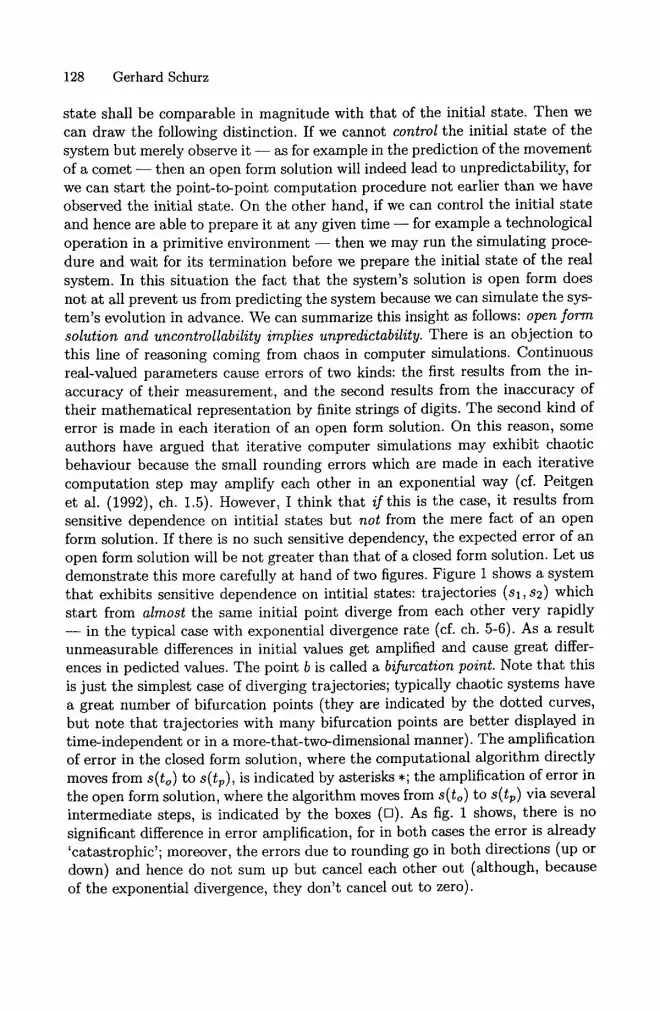
s ta te shall be comparable in magnitude with that of the initial state. Then we can draw the following distinction. If we cannot control the initial s ta te of the system but merely observe it - - as for example in the prediction of the movement of a comet - - then an open form solution wilt indeed lead to unpredictability, for we can s tar t the point-to-point computat ion procedure not earlier than we have observed the initial state. On the other hand, if we can control the initial s ta te and hence are able to prepare it at any given time - - for example a technological operat ion in a primitive environment - - then we may run the simulating procedure and wait for its termination before we prepare the initial s ta te of the real system. In this situation the fact that the system's solution is open form does not at all prevent us from predicting the system because we can simulate the sys- t em ' s evolution in advance. We can summarize this insight as follows: open form solution and uncontrolIability implies unpredictability. There is an objection to this line of reasoning coming from chaos in computer simulations. Continuous real-valued parameters cause errors of two kinds: the first results from the inaccuracy of their measurement, and the second results from the inaccuracy of their mathemat ica l representation by finite strings of digits. The second kind of error is made in each iteration of an open form solution. On this reason, some authors have argued tha t iterative computer simulations may exhibit chaotic behaviour because the small rounding errors which are made in each iterative computa t ion step may amplify each other in an exponential way (cf. Peitgen et al. (1992), ch. 1.5). However, I think tha t if this is the case, it results from sensitive dependence on intitial states but not from the mere fact of an open form solution. If there is no such sensitive dependency, the expected error of an open form solution will be not greater than tha t of a closed form solution. Let us demonst ra te this more carefully at hand of two figures. Figure 1 shows a system tha t exhibits sensitive dependence on intitial states: trajectories (sl, s2) which s tar t from almost the same initial point diverge from each other very rapidly - - in the typical case with exponential divergence rate (cf. ch. 5-6). As a result unmeasurable differences in initial values get amplified and cause great differences in pedicted values. The point b is called a bifurcation point. Note tha t this is just the simplest case of diverging trajectories; typically chaotic systems have a great number of bifurcation points (they are indicated by the dotted curves, but note tha t trajectories with many bifurcation points are bet ter displayed in t ime-independent or in a more-that-two-dimensional manner). The amplification of error in the closed form solution, where the computational algorithm directly moves from S(to) to s(tp), is indicated by asterisks *; the amplification of error in the open form solution, where the algorithm moves from S(to) to S(tp) via several intermediate steps, is indicated by the boxes ([:]). As fig. 1 shows, there is no significant difference in error amplification, for in both cases the error is already 'catastrophic ' ; moreover, the errors due to rounding go in both directions (up or down) and hence do not sum up but cancel each other out (although, because of the exponential divergence, they don' t cancel out to zero).


e I b ,

sjj

' ~ p red ic t ion t i m e v I I to t o sz

Fig. 1: Sensit ive dependence on initial condit ions because of exponen- t ia l ly diverging t rajector ies . ~ -- measurement accuracy level. * = closed form, [] = open form.

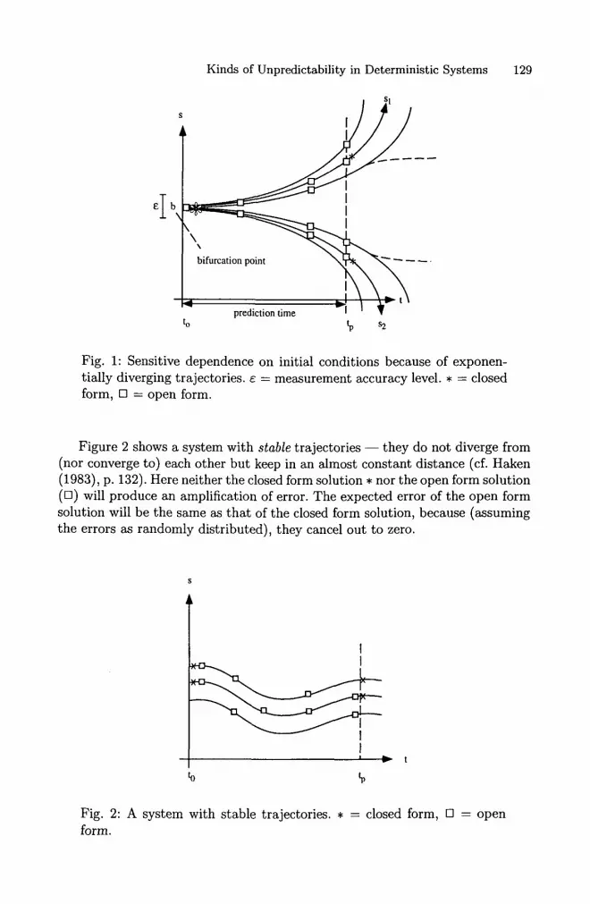
F igure 2 shows a sys tem wi th stable t ra jector ies - - they do not diverge f rom (nor converge to) each other but keep in an a lmost cons tant d is tance (cfi Haken (1983), p. 132). Here nei ther the closed form solution �9 nor the open form solut ion ([::]) will p roduce an amplif icat ion of error. The expec ted error of the open form solut ion will be the same as t h a t of the closed form solution, because (assuming the errors as r andomly dis t r ibuted) , they cancel out to zero.

$

l I

I

to

Fig. 2: A sys tem with s table trajectories. �9 = closed form, f o r m .

[] = open

130 Gerhard Schurz

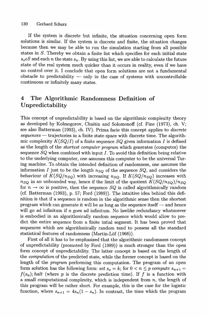
If the system is discrete but infinite, the situation concerning open form solutions is similar. If the system is discrete and finite, the situation changes because then we may be able to run the simulation starting from all possible states in S. Thereby we obtain a finite list which specifies for each initial state soeS and each n the state sn. By using this list, we are able to calculate the future state of the real system much quicker than it occurs in reality, even if we have no control over it. I conclude that open form solutions are not a fundamental obstacle to predictability - - only in the case of systems with uncontrollable continuous or infinitely many states.

4 T h e A l g o r i t h m i c R a n d o m n e s s D e f i n i t i o n o f

U n p r e d i c t a b i l i t y

This concept of unpredictability is based on the algorithmic complexity theory as developed by Kolmogorov, Chaitin and Solomonoff (cf. Fine (1973), ch. V; see also Bat terman (1993), ch. IV). Prima facie this concept applies to discrete sequences - - trajectories in a finite state space with discrete time. The algorithmic complexity K(SQ/ I ) of a finite sequence SQ given information I is defined as the length of the shortest computer program which generates (computes) the sequence SQ when combined with input I. To avoid this definition being relative to the underlying computer, one assumes this computer to be the universal Tur- ing machine. To obtain the intended definition of randomness, one assumes the information I just to be the length nsQ of the sequence SQ, and considers the behaviour of K(SQ/nsQ) with increasing nsQ. If K(SQ/nsQ) increases with nsQ in an unbounded way, hence if the limit of the quotient K(SQ/nSQ)/nSQ for n --~ cx~ is positive, then the sequence SQ is called algorithmically random (cf. Bat terman (1993), p. 57; Ford (1989)). The intuitive idea behind this definition is that if a sequence is random in the algorithmic sense then the shortest program which can generate it will be as long as the sequence i t s e l f - and hence will go ad infinitum if n goes ad infinitum. No lawlike redundancy whatsoever is embodied in an algorithmically random sequence which would allow to predict the entire sequence from a finite intial segment. It has been proved that sequences which are algorithmically random tend to possess all the standard statistical features of randomness (Martin-LSf (1966)).

First of all it has to be emphasized that the algorithmic randomness concept of unpredictability (promoted by Ford (1989)) is much stronger than the open form concept of unpredictability. The latter concept is based on the length of the computation of the predicted state, while the former concept is based on the length of the program performing this computation. The program of an open form solution has the following form: set So = k; for 0 < n <_ p compute Sn+l :

f ( sn) ; halt (where p is the discrete prediction time). If f is a function with a small computational complexity, which is independent from n, the length of this program will be rather short. For example, this is the case for the logistic function, where sn+l = 4s~(1 - s~). In contrast, the time which the program


needs to compute sn from so (via n steps) - in other words, its halting time - - may be very long, (simply because recursive commands of unit length may cause iterations of any number). In other words, that a sequence SQ is algorithmically random does not only imply that there exists no closed form solution, but also that there exists no open form solution generated by an iterative function f(s, 0 with a complexity which does not increase with n. Many open form functions do not create algorithmically random sequences. For instance, the logistic function does not produce random numbers, if it is projected on a partit ion of the unit interval into three subintervals of equal length. In this case, certain combinations of the numbers 1, 2 and 3 will never be produced by the logistic function (cf. Peitgen et al. (1992), p. 396), and hence the sequence is not random, although the function is essentially of open form, not equivalent with any closed form function.

The interesting question is how algorithmic randomness is related to sensitive dependence on initial conditons. To answer this question one first has to find a way to apply the concept of algorithmic complexity, which is defined for discrete sequences, to continuous trajectories. This is done by partitioning the continuous state space S as well as the continuous time T into a finite number of 'cells', and by considering the projection of the t rajectory on this parti t ion - - this projection is called a symbolic t rajectory (this notion was first intro- duced by Hadamard; cf. Chirikov (these proceedings), ch. 2.2). Of course the algorithmic complexity of such a symbolic t rajectory will depend on the underlying partition, but by making the partit ion finer and finer one obtains a limit algorithmic complexity which is partition-independent. It follows from theorems proved by Brudno (1983), White (1993) and Pesin (1977) that for almost all trajectories satisfying certain mathematical preconditions, their algorithmic complexity equals their metric entropy which in turn equals the sum of their positive Lyapunov exponents. 7 Thereby the Lyapunov exponents of a t ra jectory express the mean exponential rate of divergence of its nearby trajectories. If they are positive (negative), the trajecories are exponentially diverging (converging).

The Brudno-White-Pesin theorems establish a mathematical connection between algorithmic randomness and sensitive dependence on initial conditions. These theorems as well as their preconditions are highly complicated. Therefore it seems appropriate to t ry to explain the relation between algorithmic randomness (AR) and (exponentially) diverging trajectories (DT) from a purely qualitative point of view. The one direction, from DT to AR, seems to have an easy qualitative explanation. For given the trajectories are everywhere rapidly diverging from each other, then for every finite parti ton P(S) of the state space S, the information that the position of the particle at given discrete times t l , . . . , tn falls into certain cells c l , . . . , c~ of P(S) will not be sufficient tO determine its

7 Cf. Batterman (these proceedings), ch. 2; Chirikov (these proceedings), ch. 2.4. I have simplified matters: the discrete partitioning of S is needed for the definition of metric entropy, while for the definition of algorithmic complexity it suffices to consider a discrete open cover of S.

132 Gerhard Schurz

position at the next time point tn+l - two trajectories coinciding in all these cells may spread between tn and tn+l into two distinct cells. Therefore the shortest computer program which can generate the symbolic trajectory c l , . . . , c ~ will always have to contain explicit information about all the discrete position values and hence will increase with increasing n in an unbounded way. So it will be algorithmically random.

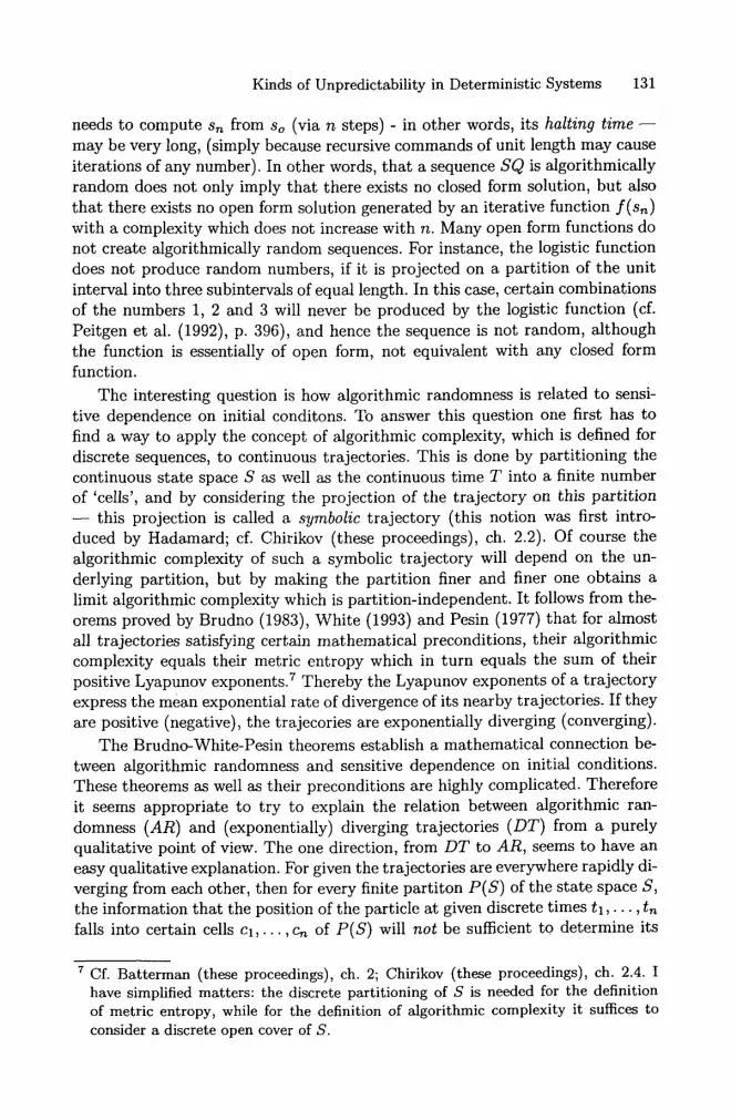
The other direction, however, cannot be explained in such a straightforward qualitative manner. It is clear tha t if we are allowed to take as our t ra jectory any function, then A R will not imply DT. As an example, assume the trajectories to be functions mapping integers (Int) into themselves - hence both state space and time are discrete and infinite. Take any noncomputable function f ( x ) and define the set of trajecories to be the set of all functions differing from f ( x ) by an integer, {g(x) [ g(x) = f ( x ) + m for some integer m}. These trajectories will be algorithmically complex, because they are not computable, although their trajectories are stable. See fig. 3.

I t I I t

Fig. 3: Algorithmically complex but stable trajectories with discrete S and T.

But recall what was said in ch. 2 concerning time-dependent Hamilton op- erators. Not just any function can count as deterministic - only one which is sufficiently 'regular'. The functions of fig. 3 are totally irregular and hence cannot constitute a violation of the claim that every deterministic function which is algorithmically random must have diverging trajectories. Indeed, the preconditions of the Brudno-White-Pesin-theorems seem to be rather strong - they require the trajectories to be a continuous, inversely continuous, twice differen- tiable and measure-preserving mapping of a compact metrizable space into itself (cf. Bat terman (these proceedings), ch. 2). I conjecture that these conditions are similar to the conditions for analytic functions, or functions representable by a Taylor series, which have been mentioned in ch. 2. For such a function f the


Brudno-White-Pesin-theorem has an easy qualitative explanation: if we let the values fn(to) of all the finitely many derivatives of f be the initial conditions, then these values determine the entire function. Hence if these values are given with some finite accuracy E, then given the trajectories are stable, the values of f for all times t will be determined up to some given ~; and so, the expression KSQ/nsQ/nsQ will go to zero for increasing nsv.

Let us finally consider the question of algorithmic randomness for systems with a discrete state space. If the state space is discrete and finite, algorithmic randomness is impossible. For then there exists a finite list C_ S • S specifying for each state in S which next state is determined by it. This list gives us a finite program which together with the given initial condition will generate the correct temporal evolution for a prediction time of arbitary length. So with increasing length of this temporal evolution (coded as a sequence), the algorithmic complexity will converge towards zero. Since every computer program is a finite and discrete system, it follows that no computer simulation can generate algorithmically random sequences, and hence that computer generated random numbers do not exist. This is important because there exist several computer algorithms for producing ' random' numbers. These computer generated 'random' numbers will always be pseudo-random, but not really random in the algorithmic sense. For similar reasons, computer generated chaos will always be pseudo-chaos in the sense explained by Chirikov (these proceedings), ch. 3.4.

Of course, if the state space is infinite, then algorithmic randomness is possible via uncomputable functions. But as was argued above, such functions can hardly be called 'deterministic'. So it seems that the only way for deterministic systems to produce random trajectories is via sensitive dependence on initial conditions because of diverging trajectories. If this is true, then deterministic unpredictability is a typical feature of continuous systems, because diverging trajectories lead to unpredictability only on the condition of limited measurement accuracy, and this condition is typical for continuous systems. In the following sections I turn to this latter concept of unpredictability. Also here we will have to face the problem that there are several different and nonequivalent concepts of trajectory divergence and, hence, of unpredictability. In ch. 5 I discuss some standard explications of t rajectory divergence. Their common feature is tha t they are based on limit considerations. In ch. 6 I will suggest some pragmatic definitions of unpredictability in order to overcome certain problems of the limit conceptions.

5 Limiting Trajectory Divergence Concepts of Unpredictability

These concepts consider the limit behaviour of trajectories - their behaviour when the difference in initial conditions goes to zero and the prediction distance goes ad infinitum.

134 Gerhard Schurz

5.1 T h e S imple T r a j e c t o r y Dive rgence C o n c e p t

This concept has been suggested by Suppes (1985), p. 192, in terms of Lyapunov- stability. A system is Lyapunov stable if two different trajectories keep arbitrarily close together, ad infinitum, provided their difference in initial conditions is sufficiently small. Let S denote the space of all possible trajectories, i.e. functions s : S --* T. Then the formal definiton of Lyapunov-stability and that of its logical contrary - (simple) trajecory divergence - are as follows. Note that the negation of (1) is logically equivalent with a condition, call it (2'), which is like (2) except that "Ve" is replaced by "3~"; but diverging trajectories will always satisfy the stronger condition (2).

(1) Lyapunov-stability: v r 3 6 > 0 Vs, s ' ~ s vt>_to: I s o - s ' l < 6 -~ I s ( t ) - s ' ( t ) l < ~ .

(2) Trajectory-divergence: w > o v~ > o 3s , s' c s 3t > to : I so - s" I< ~ A I s ( t ) - s ' ( t ) 1>>_ ~.

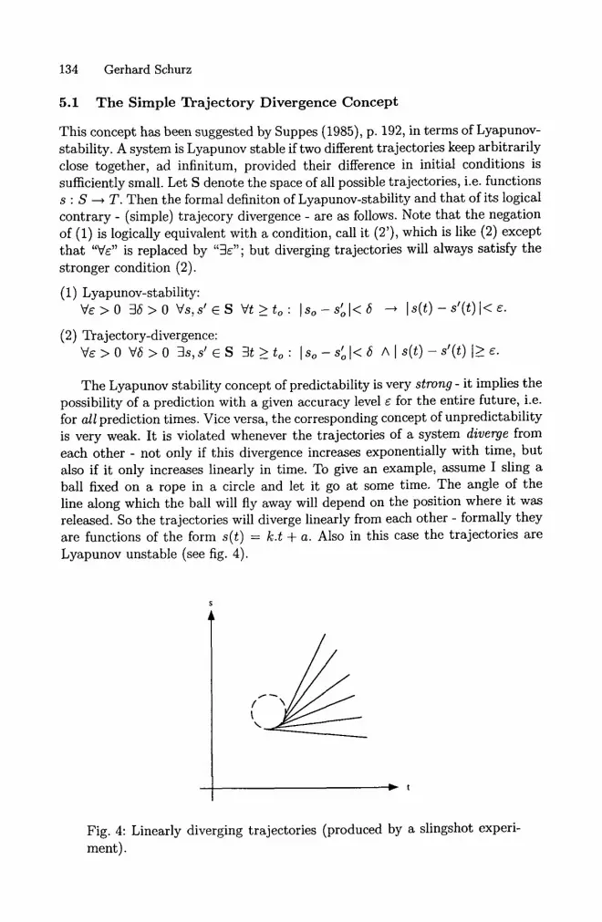
The Lyapunov stability concept of predictability is very s t r o n g - it implies the possibility of a prediction with a given accuracy level ~ for the entire future, i.e. for a l l prediction times. Vice versa, the corresponding concept of unpredictability is very weak. It is violated whenever the trajectories of a system d i v e r g e from each other - not only if this divergence increases exponentially with time, but also if it only increases linearly in time. To give an example, assume I sling a ball fixed on a rope in a circle and let it go at some time. The angle of the line along which the ball will fly away will depend on the position where it was released. So the trajectories will diverge linearly from each other - formally they are functions of the form s ( t ) = k . t + a. Also in this case the trajectories are Lyapunov unstable (see fig. 4).

t

Fig. 4: Linearly diverging trajectories (produced by a slingshot experiment).


The trajectories of fig. 4 are Lyapunov unstable and hence unpredictable according to the trajectory divergence concept. Since measurement of the release time has finite accuracy, it will not be possible to predict the ball's position with a certain accuracy c for all future times. Intuitively, however, I think one would not speak in this case of an unpredictable system. It seems that the condition is too weak.

5.2 T h e E x p o n e n t i a l D ive rgence C o n c e p t

This is a stronger concept which identifies unpredictability with exponential divergence of trajectories. It is connected with the Lyapunov coefficients which have been mentioned in ch. 4 and express the mean exponential rate of divergence of two nearby trajectories. If the trajectories diverge exponentially from each other, the Lyapunov coeffficients are positive (if they converge exponentially, the Lyapunov exponents are negative, and otherwise they are zero). Hence, this concept of unpredictability is equivalent with that of positive Lyapunov exponents. It is the concept of unpredictability which underlies the Brudno-White- Pesin theorems of explained in ch. 4.

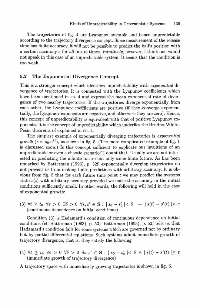
The simplest example of exponentially diverging trajectories is exponential growth (s = so.ekt), as shown in fig. 5. (The more complicated example of fig. 1 is discussed soon.) Is this concept sufficient to explicate our intuitions of an unpredictable or even a chaotic szenario? I doubt that. Usually we are not interested in predicting the infinite future but only some finite future. As has been remarked by Batterman (1993), p. 52f, exponentially diverging trajectories do not prevent us from making finite predictions with arbitrary accuracy. It is obvious from fig. 5 that for each future time point t we may predict the systems state s(t) with arbitrary accuracy provided we make the accuracy in the initial conditions sufficiently small. In other words, the following will hold in the case of exponential growth:

(3) v t > to w > o 36 > o Vs, s' c s : I so - sS I< 6 -~ Is ( t ) - s'(t ) I< (continuous dependence on initial conditions)

Condition (3) is Hadamard's condition of continuous dependence on initial conditions (cf. Batterman (1993), p. 53). Batterman (1993), p. 53f tells us that Hadamard's condition fails for some systems which are governed not by ordinary but by partial differential equations. Such systems admit immediate growth of trajectory divergence, that is, they satisfy the following

(4) vt_>to w > 0 v 6 > O 3 s , s ' ~ S : [ s o - s ~ l < 6 AIs(t)-s'(t)l_> (immediate growth of trajectory divergence)

A trajectory space with immediately growing trajectories is shown in fig. 6.

Gerhard Schurz 136

b

Fig. 5: Exponential growth. Fig. 6: Immediately growing

trajectories - condition (4).

t

Note that (4) is much stronger than the negation of (3), which is

(5) 3 t > t 0 3 , > 0 v ~ > 0 3s, s ' e S : I s 0 - s ~ l < ~ A I s ( t ) - s ' ( t ) l > E (negation of Hadamard's condition)

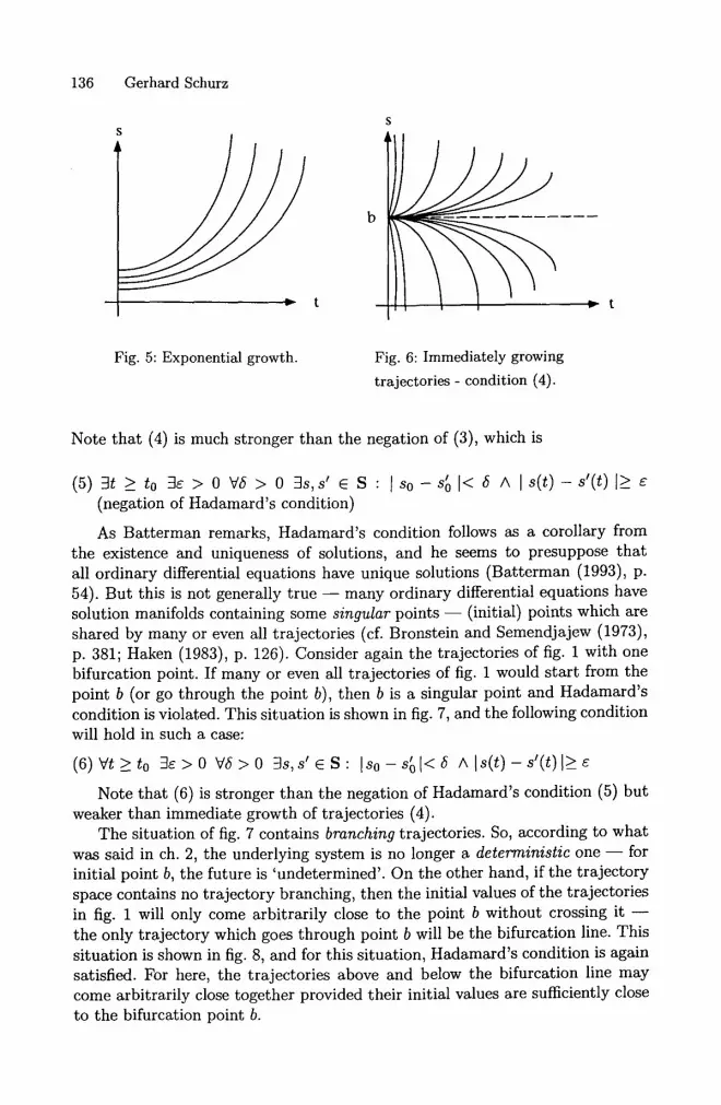
As Batterman remarks, Hadamard's condition follows as a corollary from the existence and uniqueness of solutions, and he seems to presuppose that all ordinary differential equations have unique solutions (Batterman (1993), p. 54). But this is not generally true - - many ordinary differential equations have solution manifolds containing some singular points - - (initial) points which are shared by many or even all trajectories (cf. Bronstein and Semendjajew (1973), p. 381; Haken (1983), p. 126). Consider again the trajectories of fig. 1 with one bifurcation point. If many or even all trajectories of fig. 1 would start from the point b (or go through the point b), then b is a singular point and Hadamard's condition is violated. This situation is shown in fig. 7, and the following condition will hold in such a case:

(6) V t > t 0 3 ~ > 0 V S > 0 3s, s 'ES : [so-Jol<5 AIs(t)-s'(t)l>_~

Note that (6) is stronger than the negation of Hadamard's condition (5) but weaker than immediate growth of trajectories (4).

The situation of fig. 7 contains branching trajectories. So, according to what was said in ch. 2, the underlying system is no longer a deterministic one - - for initial point b, the future is 'undetermined'. On the other hand, if the trajectory space contains no trajectory branching, then the initial values of the trajectories in fig. 1 will only come arbitrarily close to the point b without crossing it - - the only trajectory which goes through point b will be the bifurcation line. This situation is shown in fig. 8, and for this situation, Hadamard's condition is again satisfied. For here, the trajectories above and below the bifurcation line may come arbitrarily close together provided their initial values are sufficiently close to the bifurcation point b.


" t

Fig. 7: A singular point without

unique solutions - condition (6).

Fig. 8: Bifurcation without

violation of condition (3).

Hunt (1987), p. 130, has argued that whenever the t rajectory space contains a bifurcation point, Hadamard's condition will be violated. I do not know whether there exists a unique definition of the notion of a bifurcation point and what it is. However, if both figures 7 and 8 are examples of bifurcations, then Hunt 's claim cannot be generally true - it holds only for fig. 7 but not for fig. 8.

It seems to me that Batterman's claim that Hadamard's condition is generally satisfied for all ordinary differential equations is true if it is restricted to those which produce deterministic t rajectory spaces. However tha t may be, many systems usually subsumed under the rubric 'chaotic systems' satisfy Hadamard's continuity condition. Therefore, as a general condition for unpredictability the negation of Hadamard's continuity condition seems to be too strong. Hence we are confronted with a kind of dilemma. We have three explications of unpredictability in the sense of sensitive dependency on initial conditions. The first two are too weak and the third is too strong. Is there something in between which fits our intuitions better? I think that every limit concept of unpredictability will be unsatisfactory in this respect, because our intuitions of unpredictability and chaos are essentially pragmatic. We are not interested in predictions about the limit behaviour but about a finite prediction distance, and we cannot measure the initial conditions with arbitrarily high precision but only with finite precision. Also, the error in our predictions need not be made arbitrarily small, but only if it exceeds a certain relevant degree, it will be practically harmful. Based on these considerations I will suggest in the next chapter some pragmatic definitions of unpredictability.

6 Pragmatic Trajectory Divergence Concepts of Unpredictability

I make three pragmatic assumptions. First, there exists a smallest measurement accuracy ~0 of the initial conditions relative to the given background of theoreti- cal knowledge as well as the given technical possibilities. Let me emphasize that

138 Gerhard Schurz

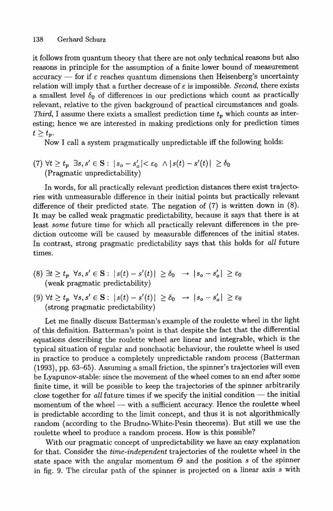
it follows from quantum theory that there are not only technical reasons but also reasons in principle for the assumption of a finite lower bound of measurement accuracy - - for if ~ reaches quantum dimensions then Heisenberg's uncertainty relation will imply that a further decrease of E is impossible. Second, there exists a smallest level s̀o of differences in our predictions which count as practically relevant, relative to the given background of practical circumstances and goals. Third, I assume there exists a smallest prediction time tp which counts as interesting; hence we are interested in making predictions only for prediction times t ~ t p .

Now I call a system pragmatically unpredictable iff the following holds:

(7) vt>tp 9s, s ' c S : Iso-S'ol<~o AIs ( t ) - s ' ( t ) l >_,So (Pragmatic unpredictability)

In words, for all practically relevant prediction distances there exist trajectories with unmeasurable difference in their initial points but practically relevant difference of their predicted state. The negation of (7) is written down in (8). It may be called weak pragmatic predictability, because it says that there is at least some future t ime for which all practically relevant differences in the prediction outcome will be caused by measurable differences of the initial states. In contrast, strong pragmatic predictability says that this holds for all future times.

(8) 3 t > tp v , , s' e s : Is ( t ) - s ' ( t ) >_ `so --* I so - s'ol >_ ~o (weak pragmatic predictability)

(9) Vt>_tp Vs, s ' c S : I s ( t ) - s ' ( t ) l _`so ~ I so-s'ol >_~o (strong pragmatic predictability)

Let me finally discuss Bat terman's example of the roulette wheel in the light of this definition. Bat terman's point is that despite the fact that the differential equations describing the roulette wheel are linear and integrable, which is the typical situation of regular and nonchaotic behaviour, the roulette wheel is used in practice to produce a completely unpredictable random process (Bat terman (1993), pp. 63-65). Assuming a small friction, the spinner's trajectories will even be Lyapunov-stable: since the movement of the wheel comes to an end after some finite time, it will be possible to keep the trajectories of the spinner arbitrarily close together for all future times if we specify the initial condition - - the initial momentum of the wheel - - with a sufficient accuracy. Hence the roulette wheel is predictable according to the limit concept, and thus it is not algorithmically random (according to the Brudno-White-Pesin theorems). But still we use the roulette wheel to produce a random process. How is this possible?

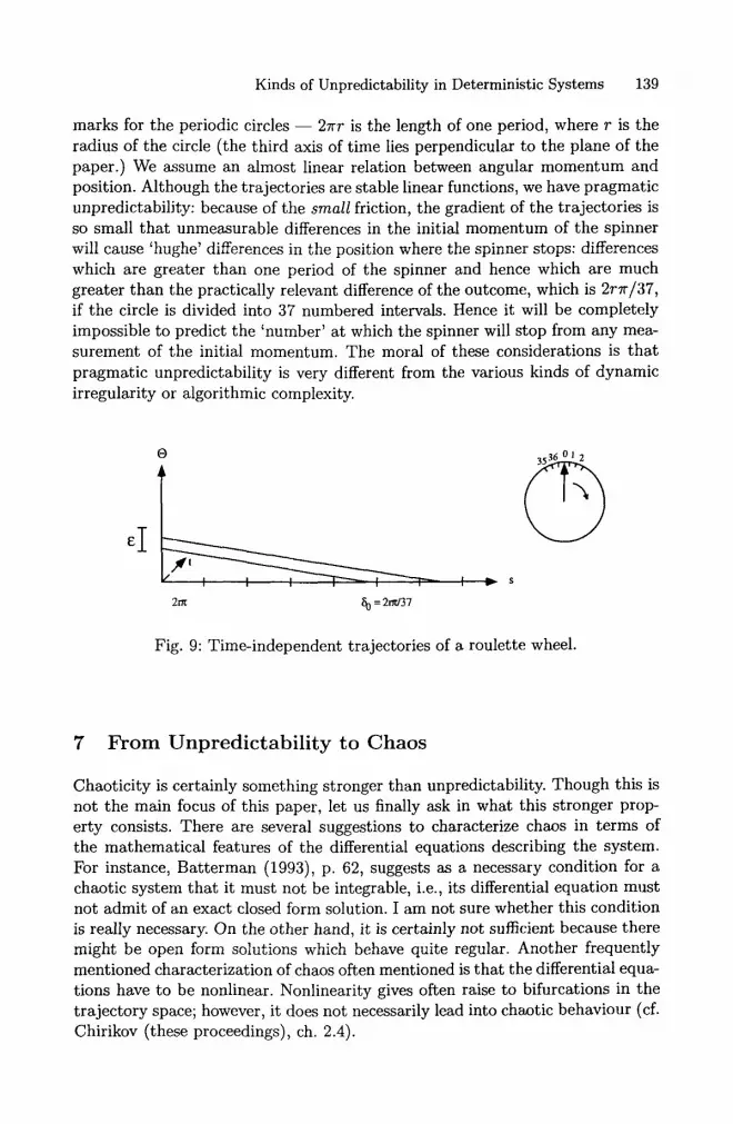
With our pragmatic concept of unpredictability we have an easy explanation for that. Consider the time-independent trajectories of the roulette wheel in the state space with the angular momentum ~ and the position s of the spinner in fig. 9. The circular path of the spinner is projected on a linear axis s with


marks for the periodic circles - - 27rr is the length of one period, where r is the radius of the circle (the third axis of time lies perpendicular to the plane of the paper.) We assume an almost linear relation between angular momentum and position. Although the trajectories are stable linear functions, we have pragmatic unpredictability: because of the small friction, the gradient of the trajectories is so small that unmeasurable differences in the initial momentum of the spinner will cause 'hughe' differences in the position where the spinner stops: differences which are greater than one period of the spinner and hence which are much greater than the practically relevant difference of the outcome, which is 2r~r/37, if the circle is divided into 37 numbered intervals. Hence it will be completely impossible to predict the 'number' at which the spinner will stop from any measurement of the initial momentum. The moral of these considerations is that pragmatic unpredictability is very different from the various kinds of dynamic irregularity or algorithmic complexity.

o

2 ~ ~0 = 2~d37

~ s

6 01 2

Fig. 9: Time-independent trajectories of a roulette wheel.

7 F r o m U n p r e d i c t a b i l i t y t o C h a o s

Chaoticity is certainly something stronger than unpredictability. Though this is not the main focus of this paper, let us finally ask in what this stronger prop- erty consists. There are several suggestions to characterize chaos in terms of the mathematical features of the differential equations describing the system. For instance, Batterman (1993), p. 62, suggests as a necessary condition for a chaotic system that it must not be integrable, i.e., its differential equation must not admit of an exact closed form solution. I am not sure whether this condition is really necessary. On the other hand, it is certainly not sufficient because there might be open form solutions which behave quite regular. Another frequently mentioned characterization of chaos often mentioned is that the differential equations have to be nonlinear. Nonlinearity gives often raise to bifurcations in the trajectory space; however, it does not necessarily lead into chaotic behaviour (cf. Chirikov (these proceedings), ch. 2.4).

140 Gerhard Schurz

I want to propose that there are three conditions which are necessary and taken together sufficient for chaos. One condition is pragmatic unpredictability. For according to the limit concept of unpredictability, i.e. the trajectory divergence concept, even our solar system is unstable and chaotic (cf. Chirikov (these proceedings), ch. 2.5), but the time after which it becomes unstable is of the same dimension as the cosmological time and hence without practical relevance. I think it makes no sense to call our solar system chaotic if we want to avaoid making the concept of chaos almost empty; therefore I think that pragmatic unpredictability is a necessary condition for chaos. But pragmatic unpredictability is not enough for chaos, as is seen from the roulette wheel: though it is pragmatically unpredictable, its trajectories are regular and stable and thus not at all chaotic. So I think that a second condition for chaos is exponential trajectory divergence, and thus, by the Brudno-White-Pesin theorems, algorithmic randomness. But also this is not enough, for intuitively we want to distinguish chaotic behaviour from exponential growth (or exponential 'explosion') - - and the trajectories describing exponential growth satisfy the second condition, and with a suitably chosen relevant outcome interval 60 also the first condition. As emphasized by Chirikov (these proceedings), ch. 2.4, the important third condition of chaos is the boundedness of the trajectories: in distinction to exponential growth, the (time-independent) trajectories remain within a finite region of the state space. This third condition explains several further characteristic features of chaotic trajectory spaces. First, the boundedness of trajectories is usually produced by adding a nonlinear term to a linear differential equation; hence the importance of nonlinearity. Second, boundedness together with algorithmic randomness implies that the (time-independent) trajectories will oscillate in a finite region of the state space without being periodic, i.e. recurrent in time (cf. Wein- gartner 1995, ch. 1.3.4); for if they were periodic, they could not be exponentially diverging from each other. This implies, third, that the 'symbolic' trajectories mentioned in ch. 4 will contain all possible sequences (Chirikov (these proceedings), ch. 2.2) and thus simulate a statistical random experiment; and fourth, that the set of trajectories starting from one finite cell will, after some time, have filled the entire state space (cf. Weingartner 1995, ch. 1.3.4).

Let me conclude with a conceptual problem. It seems to me that the third condition of boundedness is - not in conflict with the first condition of pragmatic unpredictability, but - in conflict with the second condition of trajectory divergence. For if the trajectories remain within a finite region S/ of the state space S, then it is impossible that the mean distance of neighbouring trajectories increases - linearly or exponentially - with time in an unrestricted way: the distance will never exceed the 'diameter' I Sf I of the finite region Sf. So strictly speaking, the limit definition (2) of trajectory divergence cannot be satisfied if the trajectories are bounded.

I do not know what the best solution of this problem will be. Maybe we should drop the second condition and only work with the first and the third. Alternatively, we could restrict the second condition of exponential divergence to some finite initial segment of time. However, these considerations lie beyond the scope of this paper.

References


Batterman, R. (19937: Defining Chaos. Philosophy of Science 60, 43 - 66 Batterman, R. (these proceedings): Chaos: Algorithmic Complexity versus Dynamical

Instability Bronstein, I. N., Semendjajew, K. A. (1973): Tasehenbuch der Mathematik (Verlag

Harri Deutsch, Ziirich) Brudno, A. A. (1983): Entropy and the Complexity of the Trajectories of a Dynamical

System. Transactions of the Moscow Mathematical Society 2, 127-151 Chirikov, B. (these proceedings): Natural Laws and Human Prediction Fine, T. (1973): Theories of Probability (New York, Academic Press) Ford, J. (1989): What is Chaos, That We Should be Mindful of It? In: P. Davies (ed.),

The New Physics, Cambridge Univ. Press, Cambridge, pp. 348-371 Haken, H. (1983): Synergetik. Eine Einfiihrung (Springer, Berlin) Hunt, G. M. K. (1987): Determinism, Predictability and Chaos. Analysis 47, 129-132 Martin-LSf, P. (1966): The Definition of a Random Sequence. Information and Control

9, 602-619 Peitgen, H.-O. et al. (1992): Bausteine des Chaos - Fraktale (Springer und Klett-Cotta,

Berlin and Stuttgart) Pesin, Ya. B. (1977): Characteristic Lyapunov Exponents and Smooth Ergodic Theory.

Russian Mathematical Surveys 32, 55-114 Russell, B. (1953): On the Notion of Cause In: H. Feigl and M. Brodbeck (Eds.),

Readings in the Philosophy of Science (AppletomCentury-Crofts, New York) Schurz, G. (1989): Different Relations between Explanation and Prediction in Stable,

Unstable and Indifferent Systems. In: P.Weingartner/G. Schurz (eds.), Philosophy of the Natural Sciences (Proceedings of the 13th International Wittgenstein Sympo- sium), HSlder-Pichler-Tempsky, Vienna, pp. 250-258

Stone, M. (I989): Chaos, Prediction and Laplacean Determinism. American Philosoph- ical Quarterly 26 (2), 123-131

Suppes, P. (1985): Explaining the Unpredictable. Erkenntnis 22, 187-195 Weingartner, P. (these proceedings): Under what Transformations are Laws invariant? White, H. (1993): Algorithmic Complexity of Points in Dynamical Systems. Ergodic

Theory and Dynamical Systems 13, 807-830 Zachmann, H. G. (1973): Mathematik fiir Chemiker (Verlag Chemie, Weinheim, 3rd

edition)

Documents

Kinds of unpredictability in deterministic systems