arX

iv:1

104.

3421

v1 [

cs.C

C]

18

Apr

201

1

April 19, 2011 0:12 WSPC/INSTRUCTION FILE Irreducibility

International Journal of Foundations of Computer Sciencec© World Scientific Publishing Company

EMPIRICAL ENCOUNTERS WITH COMPUTATIONAL

IRREDUCIBILITY AND UNPREDICTABILITY

HECTOR ZENIL∗

IHPST (Paris 1/CNRS/ENS Ulm)hector.zenil-chavez@malix.univ-paris1.fr

FERNANDO SOLER-TOSCANO

Grupo de Logica, Lenguaje e InformacionDepartamento de Filosofıa, Logica, y Filosofıa de la Ciencia

Universidad de Sevillafsoler@us.es

JOOST J. JOOSTEN

Departament de Logica, Historia i Filosofia de la CienciaUniversitat de Barcelona

jjoosten@us.es

Received (31 December 2010)

There are several forms of irreducibility in computing systems, ranging from undecid-ability to intractability to nonlinearity. This paper is an exploration of the conceptualissues that have arisen in the course of investigation speed-up and slowdown phenomenain small Turing machines. We present the results of a basic test that may spur othersto further explore experimental approaches to theoretical results. The test involves anattempt to shortcut the computations of a (relatively) large set of small Turing machinesby means of sequence prediction using a specialized function finder program. Among theresults, the experiment prompts an investigation into rates of convergence of decisionprocedures, the problem of extensionality and the definability of computable sets.

Keywords: Computational irreducibility; Wolfram’s PCE; problem of induction; empiri-cal predictability; halting problem; partial functions; definable sets; decision problems.

2010 Mathematics Subject Classification: 68Q01, 68Q17, 68Q15

1. Introduction

Formal uncertainty has interested thinkers for centuries. The mechanistic paradigm,

consolidated in the works of Boyle, Hooke, Newton, Laplace, among others, domi-

nated modern science replacing previous teleological explanations. Popper, however,

∗H. Zenil is also affiliated to Wolfram Research.

1

April 19, 2011 0:12 WSPC/INSTRUCTION FILE Irreducibility

2 H. Zenil, F. Soler-Toscano and J.J. Joosten

in making his case against scientific determinism[18], made an empirical distinction

between clocks and clouds with regard to their (un)predictability.

With the development of quantum mechanics and the discovery of the phe-

nomenon of hypersensitivity to initial conditions of certain (nonlinear) systems, the

fragility of the mechanistic approach–emphasizing the clockwork worldview of un-

bounded predictability–began to be apparent. While quantum mechanics (under

the standard Copenhagen interpretation), bases its unpredictability on uncertainty

at the level of the intrinsic properties of elementary particles[4], the study of non-

linear phenomena has disconnected determinism from predictability. With the help

of computer simulations, Edward Lorenz[17] found that some physical systems were

unstable with respect to small modifications. That is, after a short period of time

their behavior was unpredictable for very small changes in the initial conditions,

even if finite and fully deterministic.

Various arguments and results have been advanced as to the scope and origin of

all kinds of limits, and computer related forms of irreducibility exist that are quite

independent of physical interpretations, e.g. interpretations centered on the extent

of the resources that a system may need to carry out a computation. Indeed, some

of these irreducibility results are inherent to computing systems, as epitomized by

the undecidability of the halting problem. Turing’s Halting Problem[22] states that

there is no algorithm to determine whether a given Turing Machine on a given input

halts or keeps on calculating indefinitely.

There is another kind of irreducibility presented by Wolfram which seems to

capture a phenomenon intrinsic to the unfolding computation of a deterministic

system, and which is apparently of a type not covered by other irreducibility mea-

sures. Wolfram’s principle of irreducibility asserts that while trivial systems may

allow shortcuts in the number of steps carried out by other systems of equivalent

sophistication, most non-trivial computations cannot be sped up other than by per-

forming (nearly) every step at a faster rate. As with other principles or guiding

theses (e.g. Church’s thesis), part of this principle remains intuitive in order to be

meaningful.

1.1. The behavior of finite deterministic systems

As a result of carrying out experiments, enumerating and generating an entire sub-

class of systems in order to systematically compare their executions, Wolfram pro-

posed a heuristic classification[23, 24] of cellular automata based on observations of

typical behaviors. The classification comprises four classes given an input: evolution

leads to trivial configurations, evolution leads to periodic configurations, evolution

is chaotic, evolution leads to complicated, persistent structures. As Wolfram points

out, his classes admit different levels of prediction, while some systems may be easily

foreseeable, most non-trivial computations are hard, if not impossible, to predict.

Many systems quickly settle into simple patterns while some others generate com-

plex patterns that look computationally irreducible, meaning there are no obvious

April 19, 2011 0:12 WSPC/INSTRUCTION FILE Irreducibility

Empirical Encounters with Computational Irreducibility and Unpredictability 3

shortcuts to predict how they unfold. Unlike planet movement or electronic cir-

cuits, one can’t find the outcome by plugging numbers into equations, one seems

to be forced to run the program to see how it evolves. Wolfram suggests that rules

like these govern much of the natural world, looking apparently complex because

they reach a maximum sophistication equivalent among all complex systems, so

predictions are very difficult, if not impossible for most of them.

2. Overview of Concepts

2.1. The problem of extensionality and undefinability of sets

When describing complicated emulations of a system one issue immediately arises.

How does one know whether the evolution is actually performing the computation

that it is supposed to be emulating? When a complicated process must be used

to encode and decode the information between the two systems, how does one

ensure that the computation is not being performed by the encoding and decoding

procedures instead?

Even simple questions about the behavior of a deterministic computing system

like a cellular automaton or a Turing machine turn out to be computationally

undecidable, as proven by Turing himself through the undecidability of the halting

problem.

Partial recursive functions are a central feature of the theory of computation.

Formally, a function f : N → N ∪ (↑) is called a (partial) computable function if

there exists a Turing machine T that implements f. This means that T outputs f(x)

for x or never halts in which case f is undefined for x. The question of whether two

functions are actually the same is undecidable.

Since we are interested in investigating the average runtime impact of Turing

machines with different resources (number states) computing the same function, we

will consider a function f computed by a Turing machine T1 the equivalent of the

function g computed by T2, if the sequences of the outputs of T1 and T2 are the

same up to a certain runtime and a certain number of inputs.

2.2. Predictability in computing systems

The phase transition measure presented in [25] implies that one may, within limits,

be able to predict (using a natural Gray-code based enumeration of initial condi-

tions) the overall behavior of a system from a segment of initial inputs based on the

prior variability of the system. Will looking at the behavior of a system for certain

times and in certain cases tell you anything about the behavior of the system at a

later time and in the general case? Experience tells us we would do well to predict

future behavior on the basis of prior behavior (a Bayesian hypothesis), yet we know

this is impossible in the general case due to the halting problem.

This may also be related to Israeli and Goldenfeld’s[9] findings. They showed

that some computationally irreducible Elementary Cellular Automata (ECA) have

April 19, 2011 0:12 WSPC/INSTRUCTION FILE Irreducibility

4 H. Zenil, F. Soler-Toscano and J.J. Joosten

properties that are predictable at certain coarse-grained levels. They did so by fol-

lowing a renormalization group technique, a mathematical apparatus that allows

one to investigate the changes in a physical system as one views it at different dis-

tance scales. They sought ways to replace several cells of an automaton with a single

cell. Their prediction capabilities are, however, also bedeviled by the unavoidable

(and ultimately undecidable) induction problem of whether one can keep on pre-

dicting for all initial conditions and for any number of steps, without having to run

the system for all possible initial conditions and for an arbitrary number of steps.

The question is then under what circumstances this large-scale prediction is

possible. For Wolfram’s elementary cellular automaton (ECA) with Rule 30, for

example, this large-scale approach doesn’t seem to say that much. For many cases,

the approach may tell at most a few steps forward, meaning the behavior is not

completely chaotic, yet unpredictable in the sense that one cannot predict in gen-

eral an arbitrary number of steps ahead other than having to run step by step the

entire computation. For many, including the most random looking, overall behavior

cannot be expected to change much. One of the main features of systems in Wol-

fram’s class 4 is precisely the existence of pervasive structures that one can predict

up to a certain point. What is surprising is that in all these fully deterministic and

extremely simple systems, such as ECA, not every aspect of their evolution is triv-

ially predictable, not because of a problem of measurement or hypersensitivity but

because we don’t know whether there are any shortcuts or how to systematically

find them, if any. And some of these questions are reducible to the halting problem.

Fig. 1. In this simulation of the ECA Rule 30, each row of pixels is derived from the one above.No shortcut is known to compute all bit values of any column and row without having to run thesystem despite the extreme simplicity of the fully deterministic rule that generates it (icon on thetop).

2.3. Irreducibility measures

To understand better the content of Wolfram’s principle of computational irre-

ducibility it is necessary to introduce his principle of computational equivalence[24]

April 19, 2011 0:12 WSPC/INSTRUCTION FILE Irreducibility

Empirical Encounters with Computational Irreducibility and Unpredictability 5

(PCE for short). As set forth in [24], PCE implies that while many computations

may admit shortcuts that allow them to be performed more rapidly, most cannot

be sped up because a simulation would require roughly the same number of steps as

that of the simulated system. In other words, other than by performing every step

at a faster speed, say with a faster computer, speed up (in the number of steps)

is, in general, not possible. Wolfram’s principle of computational irreducibility then

follows because PCE asserts that while the evolution of a simple system will al-

ways be computationally reducible, the evolution of computationally sophisticated

systems will not.

In [13], Wolfram’s PCE is described in terms of Turing degrees. The problem is

to construct a natural semi-decidable intermediate set or to rule out the existence

of any such set. Sutner concludes that no natural examples of intermediate semi-

decidable sets are known to date, suggesting that if they are not engineered, one

may effectively end up with two different cases: either a system is maximally sophis-

ticated (universal) or it is too simple (and not universal), strengthening Wolfram’s

PCE. Notice that this approach does not (necessarily) make the distinction between

universal and non-universal, but stresses that in practice it may be the case that

one always ends up with one or the other. As Sutner points out, it remains to be

seen if natural examples of intermediate sets can be found.

To place Wolfram’s principle of irreducibility in the context of other computa-

tional constraints, one can think of a partial order of degrees of irreducibility, with

the strongest one imposed by the undecidability of the halting problem, followed

by finer and less constraining limitations, such as those defined by the concept

of (in)tractability, the general hierarchy of computational complexity (that is, the

computational time of a machine). Although both Wolfram’s principle and time

complexity classes are concerned with time, Wolfram’s principle is intrinsic to the

computer system in that it is independent of any external resource such as the input

of the system, unlike time complexity. Time complexity is an asymptotical measure

dependent on the length of the inputs. One cannot say, however, whether a machine

with empty input belongs to a particular time complexity class, while Wolfram’s

irreducibility question does still apply. It is also worth noting that while Wolfram’s

principle is intrinsic, in the sense that it does not depend on the length of the in-

put, it does depend on an extrinsic resource, that is, on an observer (e.g. another

machine) looking at the original system and trying to shortcut its computation.

While the concept of universality is precisely a machine capable of carrying out

the computation of another machine by reading the latter’s transition rules table,

the universal machine is passive in the sense that it does nothing but emulate the

program it was supplied with. Wolfram’s principle, however, introduces a subjec-

tive third element, that of an active observer (even if the observer is just another

machine) that, instead of carrying out a computation, tries to outrun it.

April 19, 2011 0:12 WSPC/INSTRUCTION FILE Irreducibility

6 H. Zenil, F. Soler-Toscano and J.J. Joosten

2.4. An epistemic principle: unpredictability vs. empirical

unpredictability

An example of a predictability result that may turn out to be meaningless in practice

is Shor’s algorithm for factorization of primes in polynomial time (in quantum

computation), which according to Levin[15] may require physical precision up to

hundreds of decimals in order to work. While in theoretical computer science this is

one of many results that one may assume to be meaningful (e.g. the prediction that

RSA encryption would be jeopardized by quantum computers), there seems to be a

gap between what may be predictable in theory and what is predictable in practice.

As another illustration, one can think of the open question P=NP? Whether a

positive answer provides the actual P algorithm to solve any NP problem may

depend on the kind of proof supplied for P = NP . If the proof is constructive, it

may provide the means to find/construct the P algorithm, whereas if the proof is

axiomatic only, it may suffer from a lack of correspondence with the real world.

There have been attempts to address epistemological questions using informa-

tion theory and computer experiments to explain a theoretical result. The underly-

ing idea is not new and comes from Hume, Leibniz and Hobbes, to name but three.

The principle on which all these endeavors are based is that one really understands

something if one is able to write a computer program. By writing a program one

has first to find a precise way to describe the problem and then devise an algorithm

to carry out the computation towards the solution. To arrive to the solution one

has then to run a machine on the written program.

In the case of a computation that does halt, one can always verify that this is so

by actually performing the computation (assuming the availability of as much time

as may be needed), and then waiting for it to halt (of course, if the computation

never halts, then one will wait forever). On the other hand, if a computational

system is irreducible, one cannot say whether it will halt, whereas if it is reducible,

one may know whether it will halt without running the entire computation.

Finding a shortcut of a computation does not falsify Wolfram’s principle, because

in order to falsify the principle one would need to show that there is a shortcut for

every computation. Yet we already know that this is not true because of the halting

problem.

By solving the halting problem (for a given machineM , let’s say one can know in

advance whether M will halt or not) one may expect to be able to solve Wolfram’s

irreducibility, because one can encode the input/output pair of a system in a halting

question through its characteristic function (a function that returns “yes” or “no”).

However, the decidability of the halting problem does not tell, independently of its

time complexity, whether the system allows shortcuts in the number of computing

steps.

One can devise a test using a characteristic function of M in order to decide

whether a machine M ′ can output s from i in fewer steps. One has still to propose

s in advance in order to know, through its characteristic function, whether M

April 19, 2011 0:12 WSPC/INSTRUCTION FILE Irreducibility

Empirical Encounters with Computational Irreducibility and Unpredictability 7

produces s from i. In other words, there may not be a way to compute the function

f (f(M(i) = s) = “yes” or f(M(i) 6= s) = “no”) without having to run M at least

once. But Wolfram’s irreducibility principle tells not only that this will be often the

case, but that even knowing s devising M ′ to reduce the number of steps for any

arbitrary number of steps of M is hard (if not impossible).

For example, after years of investigation, whether a formula for predicting the

evolution of the central column of the elementary cellular automata with Rule 30

for any given time exists, is still an open problem. And even if Rule 30 does have

a formula that without having to run most steps of the automaton can provide the

state of the evolution of the rule at any given state, the principle suggests that there

will always be many more systems than known formulas to outrun thema.

2.4.1. Connections to Bennett’s logical depth and Solomonoff’s induction

problem

The connection to predictability by way of algorithmic complexity is interesting and

opportune if we are to place Wolfram’s principle of irreducibility in the context of

complexity measures. The first obvious connection is that between a reducible com-

putation and predictability, since for a computation to be predictable it has to be

reducible and vice versa. By way of algorithmic (program-size) complexity, one can

formally relate the reducible to the algorithmically predictable and algorithmically

compressible, and likewise irreducibility to unpredictability and incompressibility

in the algorithmic sense.

Let’s say that one finds a shortcut in a computation. The shortcut does not

necessarily imply that a shorter program can be devised to perform the same com-

putation; it only means that the history of the computation may be shorter. In

this sense Wolfram’s measure is closer to Bennett’s concept of logical depth[2, 3].

Bennett’s logical depth was intended to define a complexity measure by taking into

account the history of a computation from its plausible origin–assuming that its

plausible origin is likely to be the simplest (shortest) possible program (this is how

Bennett’s measure of logical depth is related to program-size complexity).

Algorithmic probability was introduced by Solomonoff[21], independently sug-

gested by Putnam[19] in relation to the problem of inductive inference, and later

formalized in Levin’s semi-measure. Levin’s m(s) is the probability of producing a

string s with a random program p when running on a universal (prefix-freeb) Tur-

ing machine. Formally, m(s) = Σp:M(p)=s2−|p|, i.e. the sum over all the programs

aAn example of a computation that turned out, after all and by serendipity, to have a shortcut isthe calculation of the digits of the constant π for which formulas from computer experiments arenow known as BPP-type formulas[1]. These require no calculation of previous digits to retrieveany digit of π in any 2n base. It is unknown today if a formula exists for the general arbitrarybase, or whether independent formulas exist for other bases.bThat is, a machine for which a valid program is never the beginning of any other program, sothat one can define a convergent probability the sum of which is at most 1.

April 19, 2011 0:12 WSPC/INSTRUCTION FILE Irreducibility

8 H. Zenil, F. Soler-Toscano and J.J. Joosten

for which M with p outputs the string s and halts. As p is itself a binary string,

m(s) is the probability that the output of M is s when provided with a sequence of

fair coin flip inputs as a programc. The algorithmic complexity CM (s) of a string

s with respect to a universal Turing machine M , measured in bits, is defined as

the length in bits of the shortest Turing machine M that produces the string s and

halts[21, 11, 14, 6].

In Wolfram’s PCE, a non-trivial computation cannot be associated with a mea-

sure of program-size complexity because objects may have low algorithmic com-

plexity (a short program that produces a complex output) yet have a complicated

evolution which is difficult to outrun, as found by Wolfram himself. In this sense,

Wolfram disconnects what algorithmic information theory succeeds in connecting

by way of infinite sequences, viz. incompressibility and unpredictability[20]. What

Wolfram’s principle would assert is that a short program yielding a long output

does not guarantee practical predictability, because either the program will require

that most of the 0 to t − 1 previous steps be performed before the state of the

system at a time t can be known, or else one would be unable, in practice, to come

up with any means to predict more than a few steps ahead in the general case.

One may, however, associate a non-trivial computation with the algorithmic

probability of its output, and attempt to formalize the concept of computational

(non) triviality. Let’s say that a computation keeps producing an output of alternat-

ing 1s and 0s. Solomonoff’s algorithmic induction would indicate that, if no other

information about the system is available, the best possible bet after n repetitions

of (01)n is that the computation will continue in the same fashion. Therefore it will

produce another “01” segment. In other words, patterns are favored, and this is how

the concept is related to algorithmic complexity–because a computation with low

algorithmic randomness will present more patterns. And according to algorithmic

probability, a machine will more likely produce and keep (re)producing the same

pattern. However, the noncalculability of the algorithmic probability of a string im-

poses another irreducibility result related to the halting problem, but extending to

the output of a Turing machine. It states that no Turing machine can compute, with

total certainty, the i-th bit of a random string based on its first i − 1 bits. Hence

in a way this is an upper bound of Wolfram’s irreducibility principle, meaning that

one cannot, even in theory, outrun any system for any arbitrary number of steps.

What Wolfram’s principle adds is that in general there will be no practical means

to outrun the system except by a few steps.

This is the question of practical predictability. Some programs, such as Wol-

fram’s Rule 30, for example, are very simple in their description–the upper limit of

the program-size complexity of Rule 30 is 8 bits (what it takes to write down the

encoding of the automaton rule in binary). Yet no formula is known to outrun the

output of the central column of Rule 30 at any time t without having to compute

cm is related to the concept of algorithmic complexity in that m(s) is at least the maximum termin the summation of programs, which is 2−C(s).

April 19, 2011 0:12 WSPC/INSTRUCTION FILE Irreducibility

Empirical Encounters with Computational Irreducibility and Unpredictability 9

most of the t − 1 previous steps. Which doesn’t mean that such a formula does

not exist. But the fact that Wolfram’s principle remains epistemological in nature

suggests that if such a formula exists it may be very hard to find. Even if it were to

be found, one could easily find another program producing similar random-looking

behavior that has no known formula to shortcut its evolution.

3. The experiment

We devised an experimental approach consisting of a battery of basic tests that

may stimulate further empirical investigation into this kind of computational irre-

ducibility. The tests shed light on concepts ultimately related to empirical versions

of the rate of convergence of decision procedures, the problem of extensionality and

undefinability, and other empirically irreducible properties of systems in general.

The tests consist of having an algorithm try to foresee a computation, given a

certain computational history. By Levin’s semi-measurem(s), we know that one can

construct a prior distribution based on this computational history, and that there

is no better way (with no other information available) to predict an output than

by using m(s). But m(s) is not computabled. The alternative option is therefore

to apply a battery of known algorithms to a sequence of outputs to see whether

the next output can be predicted. The obvious thing to do is to try to capture the

behavior of various systems and see whether one can say something about their

future evolution. This is the approach we adopt.

We will often refer to the collection of Turing machines with n states and 2

symbols as a Turing machine space denoted by (n,2). We run all the one-sided

Turing machines in (2,2) and (3,2) for 1000 steps for the first 21 input values

0, 1, . . . , 20. If a Turing machine does not halt by 1000 steps we say that it diverges

(the computation doesn’t reach a value upon halting).

Clearly, at the outset of this project we needed to decide on at least the following

issues:

(1) How to represent numbers on a Turing machine.

(2) How to decide which function is computed by a particular Turing machine.

(3) How to decide when a computation is to be considered finished.

We collect all the functions for the 21 inputs and compare the time complexity

classes, the number of outputs and the number of different functions computed

between (2,2) and (3,2), as well as the number of outputs to determine what function

a machine is computing.

3.1. Formalism

In our experiment we have chosen to work with deterministic one-sided single-tape

Turing machines, as we have done before[10] for experiments on trade-offs between

dAlthough it is approachable for some cases of limited size, as shown in [8]

April 19, 2011 0:12 WSPC/INSTRUCTION FILE Irreducibility

10 H. Zenil, F. Soler-Toscano and J.J. Joosten

time and program-size complexity. That is to say, we work with Turing machines

with a tape that is unlimited to the left but limited on the right-hand side. One-

sided Turing machines are a common convention in the literature, perhaps second

only after the other common two-sided convention. The following considerations

led us to work with one-sided Turing machines, which we found more suitable than

other configurations for our experiment.

There are (2sk)sk s-state k-symbol one-sided tape Turing machines. That means

4 096 in (2,2) and 2 985 984 in (3,2). The number of Turing machines grows expo-

nentially when adding states. For representing the data without having to store

the actual outputs that were likely to rapidly exceed our hardware capabilities, we

needed to devise a representation scheme that was efficient with regard to optimiz-

ing space (hence non-unary). On a one-sided tape which is unlimited to the left,

but limited on the right, interpreting a tape content that is almost uniformly zero

is straightforward. For example, the tape . . . 00101 would be interpreted as a binary

string read as 5 in base 10. The interpretation of a digit depends on its position

in the number. e.g. in the decimal number 121, the leftmost 1 corresponds to the

hundredths, the 2 to the tenths, and the rightmost 1 to the units. For a two-sided

infinite tape one can think of many ways to come up with a representation, but all

seem rather arbitrary.

With a one-sided tape there is no need for an extra halting state. We say that

a computation simply halts whenever the head “drops off” the right hand side of

the tape. That is, when the head is on the cell on the extreme right and receives

the instruction to move right. A two-way unbounded tape would require an extra

halting state, which in light of these considerations is undesirable. By exploring a

whole finite class, one avoids the choice of an enumeration that is always arbitrary or

hard to justify otherwise. This is because the actual enumeration in our exhaustive

approach is not relevant, thereby ensuring that we go through each of the machines

in the given space once and only once. Of course this is feasible because every (n,2)

space is finite.

On the basis of these considerations, and the fact that work has been done along

the lines of this experiment[24], we decided to fix this Turing machine formalism

and choose the one-way tape model.

3.2. Input/output representation

Once we had chosen to work with one-way single-tape Turing machines, the next

choice concerned how to represent the input values of the function. When working

with two symbol machines, there are basically two choices to be made: unary or

binary. However, there is a very subtle difference if the input is represented in binary.

If we choose a binary representation of the input, the class of functions that can be

computed is rather unnatural and very limited.

Suppose that a Turing machine on input x performs a certain computation.

Then the Turing machine will perform the very same computation for any input

April 19, 2011 0:12 WSPC/INSTRUCTION FILE Irreducibility

Empirical Encounters with Computational Irreducibility and Unpredictability 11

that is the same as x on all the cells that were re-visited by the computation. That

is, the computation will be the same for an infinitude of other inputs, thus limiting

the class of functions very severely. Hence it will be unlikely that some universal

function can be computed for any natural notion of universality.

On the basis of these considerations, we decided to represent the input in unary.

Moreover, from a theoretical standpoint it is desirable that the empty tape input

be different from the zero input. Thus the final choice for our input representation

was to represent the number x by x + 1 consecutive 1s. This way of representing

the input has two serious draw-backs:

(1) The input is very homogeneous. Thus it may happen that Turing machines that

otherwise manifest very rich and interesting behavior do not do so when the

input consists of a consecutive block of 1’s.

(2) The input is lengthy, so that runtimes can grow seriously out of hand.

None of the considerations for the input conventions applies to the output con-

vention. It is wise to adhere to an output convention that reflects as much infor-

mation about the final tape-configuration as possible. Clearly, by interpreting the

output as a binary string, the output tape configuration can be reconstructed from

the input value. Thus our outputs, for the purposes of the experiment generally and

so as to enable the use of the predictor program, will be read as binary numbers

and will be represented in decimals. The process is reversible and no information is

lost between different output transformations.

3.3. Halting condition and defining the computed function

The general question of whether a function is defined by the computation of partic-

ular Turing machine is undecidable because there is no general finite procedure to

verify that M(x) = f(x) for all x. Whether two Turing machines define the same

function is undecidable for the same reason. As convention we say then that a Tur-

ing machine M computes a function f if M(x) = f(x) for a finite number of inputs

x, with M(x) the output written on the tape by M upon halting. One also has to

impose some restrictions on the number of steps allowed and weaken the definition

of a function computed by a Turing machine. As mentioned before, we simply say

that if a machine does not halt by 1000 steps, then it diverges (meaning only that it

has not converged to any value by this number of steps). Theory tells us that when

we let the machine run further the probability of halting drops exponentially[5]. As

a result of proceeding in this way, we may see that certain functions grow fast and

regularly up to a certain point and then begin to diverge, because after some initial

values the computations were meant to halt after the imposed limit of 1000 steps.

We decided to complete these obvious non-genuine divergers manually. While for

the theoretical reasons explained above one cannot guarantee that this completion

process is flawless, error was reduced by comparing the manual completion with

the confirmation of the results by running the system for a few more steps. We

April 19, 2011 0:12 WSPC/INSTRUCTION FILE Irreducibility

12 H. Zenil, F. Soler-Toscano and J.J. Joosten

are fully aware that errors may have occurred in the completion, and they can-

not be excluded. However, the approximation we arrive at by deciding the halting

problem and running all machines upon halting is better than doing nothing and

making comparisons among incomplete data. By “manually completing” we mean

the formal method we describe in Section 3.4.

As explained before, will consider two Turing machines to have calculated the

same function if, (after completion) they compute the same outputs (even if diver-

gent in some value points) on the first 21 inputs, 0 through 20 in unary, with a

runtime bound and after completion. The result is a sequence of 21 values, one for

each of the 21 unary inputs. For 21 inputs this means that 86 016 and 62 705 664

machines run up to 1000 steps each for (2,2) and (3,2), for which a program written

in C running on a supercomputer with 24 cpu’s was used, taking about 3 hours

each for a total of 70 cpu hours.

Interestingly, we found that only a few values were needed for determining a

sequence; we did not actually have to compute all 21 values in both the space

(2,2) and the space (3,2), although we did because there was no way to know this

beforehand.

Table 1. Definability of sets in (2,2).

Sequence type total cases definable byfirst n inputs

functions 74 3runtimes 49 3

space usages 24 3

all 236 4

Table 2. Definability of sets in (3,2).

Sequence type total cases definable byfirst n inputs

functions 3886 8runtimes 3676 10

space usages 763 11

all 8222 11

Tables 1 and 2 show that algorithms (that is, output sequences together with

runtimes and tape space usages) in (2,2) and (3,2) are completely determined by

the first 4 and 11 values out of 21, which means that it suffices to compute 4 and

11 inputs to know what function in (2,2) and (3,2) is being computed. Likewise,

functions (that is output sequences only) are defined by the first 3 and 8 sequence

April 19, 2011 0:12 WSPC/INSTRUCTION FILE Irreducibility

Empirical Encounters with Computational Irreducibility and Unpredictability 13

values only.

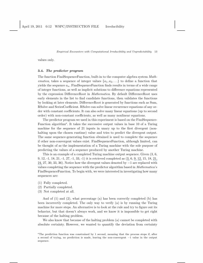
3.4. The predictor program

The function FindSequenceFunction, built-in to the computer algebra system Math-

ematica, takes a sequence of integer values {a1, a2, . . .} to define a function that

yields the sequence an. FindSequenceFunction finds results in terms of a wide range

of integer functions, as well as implicit solutions to difference equations represented

by the expression DifferenceRoot in Mathematica. By default DifferenceRoot uses

early elements in the list to find candidate functions, then validates the functions

by looking at later elements. DifferenceRoot is generated by functions such as Sum,

RSolve and SeriesCoefficient. RSolve can solve linear recurrence equations of any or-

der with constant coefficients. It can also solve many linear equations (up to second

order) with non-constant coefficients, as well as many nonlinear equations.

The predictor program we used in this experiment is based on the FindSequence-

Function algorithme. It takes the successive output values in base 10 of a Turing

machine for the sequence of 21 inputs in unary up to the first divergent (non-

halting upon the chosen runtime) value and tries to predict the divergent output.

The same sequence-generating function obtained is used to complete the sequence

if other non-convergent values exist. FindSequenceFunction, although limited, can

be thought of as the implementation of a Turing machine with the sole purpose of

predicting the values of a sequence produced by another Turing machine.

This is an example of a completed Turing machine output sequence. Given (3, 6,

9, 12, -1, 18, 21, -1, 27, -1, 33, -1) it is retrieved completed as (3, 6, 9, 12, 15, 18, 21,

24, 27, 30, 33, 36). Notice how the divergent values denoted by −1 are replaced with

values completing the sequence with the predictor algorithm based inMathematica’s

FindSequenceFunction. To begin with, we were interested in investigating how many

sequences are:

(1) Fully completed.

(2) Partially completed.

(3) Not completed at all.

And of (1) and (2), what percentage (a) has been correctly completed (b) has

been incorrectly completed. The only way to verify (a) is by running the Turing

machine for more steps. An alternative is to look at the rule and try to figure out its

behavior, but that doesn’t always work, and we know it is impossible to get right

because of the halting problem.

We also know that because of the halting problem (a) cannot be completed with

absolute certainty. However, we wanted to quantify the deviation from certainty

eThe prediction function was constrained by 1 second, meaning that the process stops if, aftera second of trying, no prediction is made, leaving the non-convergent −1 value in the outputsequence.

April 19, 2011 0:12 WSPC/INSTRUCTION FILE Irreducibility

14 H. Zenil, F. Soler-Toscano and J.J. Joosten

and ascertain whether the process managed to partially complete some divergent

values of some sequences. We ran the Turing machines up to 20 000, and for some

cases more steps, to see whether we had managed to shortcut the computation.

An objection that may be raised here is that the function design may favor

certain sequences over others. This is certainly the case, and it could be that the

particular set of algorithms is such that they are unable to partially complete a

sequence. The objection would thus not be entirely invalid and would seem to ap-

ply to any prediction procedure devised. Let’s see, however, what we mean by a

partially completed sequence. The predictor function is defined in such a way that

it either finds the sequence-generating function or it does not. If it does, nothing

prevents it from calculating any value, other than perhaps constraints on the hard-

ware (Mathematica is machine-precision dependent only). If the function does not

find the sequence-generating function, then it won’t calculate any value, leaving no

room for partial completion. To work around this problem, we also focused on the

sequences completed incorrectly. To this end, we ran the machines for further steps

and compared them, then fed the predictor once again with more values. It may also

be that machines in (3,2) are all computationally too simple even for non-empty

inputs, in which case we would like to instigate further experiments. However, even

if too simple, there were eight cases in (3,2) in which the predictor program could

not complete the sequences. These were cases in which Turing machines used the

greatest amount of resources among all, with the greatest runtimes and space usages

as shown in Table 3. The predictor program, however, allowed us to identify these

cases by failing to completing them.

Table 3. Maximum runtimes andspace usages in the sequences pro-duced by (3,2).

machine spaceno. runtime usage

582 281 8 400 889 4116

582 263 1 687 273 2068599 063 894 481 409 27 3041 031 019 2 621 435 561 233 829 2 103 293 20681 241 010 774 333 15241 233 815 1 687 273 20681 716 199 260 615 886

The authors are also currently undertaking an investigation of a sample from

(4,2)f . This work may serve as a basis for further experiments on larger spaces.

fAn exhaustive investigation is no longer possible because the space is too large even by currentcomputing standards.

April 19, 2011 0:12 WSPC/INSTRUCTION FILE Irreducibility

Empirical Encounters with Computational Irreducibility and Unpredictability 15

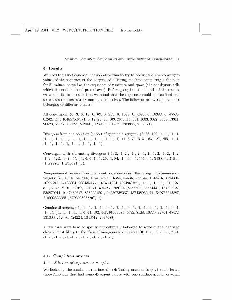
4. Results

We used the FindSequenceFunction algorithm to try to predict the non-convergent

values of the sequence of the outputs of a Turing machine computing a function

for 21 values, as well as the sequences of runtimes and space (the contiguous cells

which the machine head passed over). Before going into the details of the results,

we would like to mention that we found that the sequences could be classified into

six classes (not necessarily mutually exclusive). The following are typical examples

belonging to different classes:

All-convergent: (0, 3, 0, 15, 0, 63, 0, 255, 0, 1023, 0, 4095, 0, 16383, 0, 65535,

0,262143, 0,1048575,0), (1, 6, 12, 25, 51, 103, 207, 415, 831, 1663, 3327, 6655, 13311,

26623, 53247, 106495, 212991, 425983, 851967, 1703935, 3407871).

Divergers from one point on (subset of genuine divergers): (6, 63, 126, -1, -1, -1, -1,

-1, -1, -1, -1, -1, - 1, -1, -1, -1, -1, -1, -1, -1, -1), (1, 3, 7, 15, 31, 63, 127, 255, -1, -1,

-1, -1, -1, -1, -1, -1, -1, -1, -1, -1, -1).

Convergers with alternating divergers: (-1, 2, -1, 2 , -1 , 2, -1, 2, -1, 2, -1, 2, -1, 2,

-1, 2, -1, 2, -1, 2, -1), (-1, 0, 0, 4, -1, 20, -1, 84, -1, 340, -1, 1364, -1, 5460, -1, 21844,

-1 ,87380, -1 ,349524, -1).

Non-genuine divergers from one point on, sometimes alternating with genuine di-

vergers: (-1, 4, 16, 64, 256, 1024, 4096, 16384, 65536, 262144, 1048576, 4194304,

16777216, 67108864, 268435456, 1073741824, 4294967296, -1, -1, -1, -1), (31, 127,

511, 2047, 8191, 32767, 131071, 524287, 2097151,8388607, 33554431, 134217727,

536870911, 2147483647, 8589934591, 34359738367, 137438953471, 549755813887,

2199023255551, 8796093022207, -1).

Genuine divergers: (-1, -1, -1, -1, -1, -1, -1, -1, -1, -1, -1, -1, -1, -1, -1, -1, -1, -1, -1,

-1, -1), (-1, -1, -1, -1, -1, 0, 64, 192, 448, 960, 1984, 4032, 8128, 16320, 32704, 65472,

131008, 262080, 524224, 1048512, 2097088).

A few cases were hard to specify but definitely belonged to some of the identified

classes, most likely to the class of non-genuine divergers: (0, 1, -1, 3, -1, -1, 7, -1,

-1, -1, -1, -1, -1, -1, -1, -1, -1, -1, -1, -1, -1).

4.1. Completion process

4.1.1. Selection of sequences to complete

We looked at the maximum runtime of each Turing machine in (3,2) and selected

those functions that had some divergent values with one runtime greater or equal

April 19, 2011 0:12 WSPC/INSTRUCTION FILE Irreducibility

16 H. Zenil, F. Soler-Toscano and J.J. Joosten

Table 4. Summary of detected cases (not necessarily mutually exclusive) offunctions computed by all (3,2) Turing machines.

Computation type No. of cases fraction

All-convergent 2500 0.62Alternating convergent/divergent 383 0.095

Genuine diverger 1276 0.32Alternating non-genuine diverger/true diverger 236 0.059

Among all non-genuine divergers, 0.81%

of them converged after 20 000 steps,

which means we most likely identified

all non-genuine divergers. In the end,

among the completed Turing machines

only eight didn’t match the second pre-

diction (were not completed) and needed

to run as many as 109 steps to halt,

with the exact greatest halting times

894 481 409< 109.

Fig. 2. Breakdown of cases after manual in-spection of output sequences of Turing ma-chines with runtime bound of 1000 steps be-fore completion process (alternating means di-vergent and convergent values combined).

to 480 steps. Among the 3368 Turing machines computed in (3,2) after 1000 steps,

there are 248 divergent sequences (i.e. Turing machines that did not halt up to that

runtime for at least one of the 21 inputs defining the function) and had at least

one convergent value taking at least 480 steps. We chose this runtime to explore

because we found that computations with close to maximal runtimes (1000 steps)

were likely to be trivial (e.g. computations that go straight over the tape printing

the same symbol) and therefore less interesting (and easy) to complete (something

that we verified by sampling a subset of these machines). Moreover, after further

calculation, these computations were found to be likely true divergers, because we

ran them for 4000 steps with no new values produced.

We call a prediction the process of completing the sequences of function outputs,

runtimes and space usages of a Turing machine over the 21 inputs as described in

3. The process of predicting all the sequences (output, runtime, space usage) of a

Turing machine for 21 inputs is obviously a greater requirement than predicting a

single of these sequences (e.g. the output). Predicting the three sequences of a Turing

machine for the 21 values is equivalent to predicting the exact path to compute an

outcome, in other words, the exact algorithm.

April 19, 2011 0:12 WSPC/INSTRUCTION FILE Irreducibility

Empirical Encounters with Computational Irreducibility and Unpredictability 17

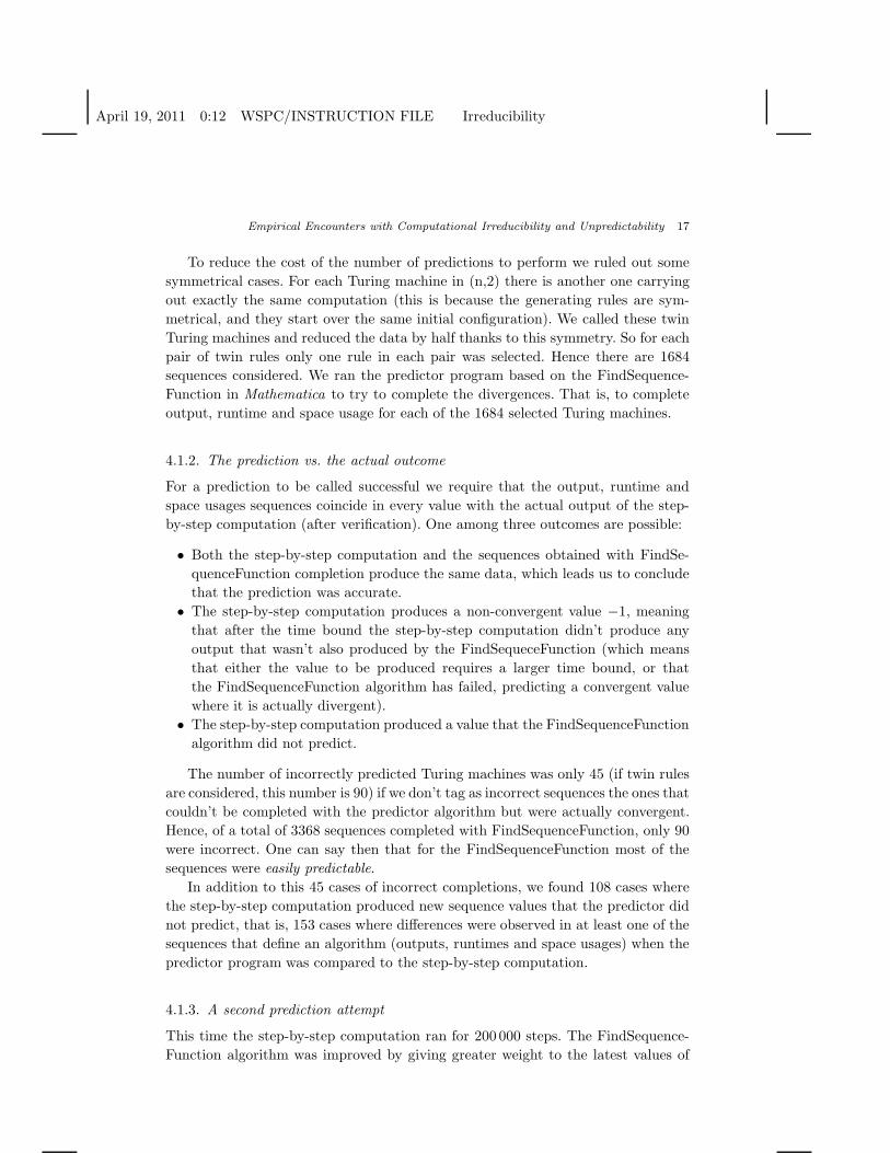
To reduce the cost of the number of predictions to perform we ruled out some

symmetrical cases. For each Turing machine in (n,2) there is another one carrying

out exactly the same computation (this is because the generating rules are sym-

metrical, and they start over the same initial configuration). We called these twin

Turing machines and reduced the data by half thanks to this symmetry. So for each

pair of twin rules only one rule in each pair was selected. Hence there are 1684

sequences considered. We ran the predictor program based on the FindSequence-

Function in Mathematica to try to complete the divergences. That is, to complete

output, runtime and space usage for each of the 1684 selected Turing machines.

4.1.2. The prediction vs. the actual outcome

For a prediction to be called successful we require that the output, runtime and

space usages sequences coincide in every value with the actual output of the step-

by-step computation (after verification). One among three outcomes are possible:

• Both the step-by-step computation and the sequences obtained with FindSe-

quenceFunction completion produce the same data, which leads us to conclude

that the prediction was accurate.

• The step-by-step computation produces a non-convergent value −1, meaning

that after the time bound the step-by-step computation didn’t produce any

output that wasn’t also produced by the FindSequeceFunction (which means

that either the value to be produced requires a larger time bound, or that

the FindSequenceFunction algorithm has failed, predicting a convergent value

where it is actually divergent).

• The step-by-step computation produced a value that the FindSequenceFunction

algorithm did not predict.

The number of incorrectly predicted Turing machines was only 45 (if twin rules

are considered, this number is 90) if we don’t tag as incorrect sequences the ones that

couldn’t be completed with the predictor algorithm but were actually convergent.

Hence, of a total of 3368 sequences completed with FindSequenceFunction, only 90

were incorrect. One can say then that for the FindSequenceFunction most of the

sequences were easily predictable.

In addition to this 45 cases of incorrect completions, we found 108 cases where

the step-by-step computation produced new sequence values that the predictor did

not predict, that is, 153 cases where differences were observed in at least one of the

sequences that define an algorithm (outputs, runtimes and space usages) when the

predictor program was compared to the step-by-step computation.

4.1.3. A second prediction attempt

This time the step-by-step computation ran for 200 000 steps. The FindSequence-

Function algorithm was improved by giving greater weight to the latest values of

April 19, 2011 0:12 WSPC/INSTRUCTION FILE Irreducibility

18 H. Zenil, F. Soler-Toscano and J.J. Joosten

the sequences and less to the earliest. That is, the closer to the prediction time the

greater relevance the values of the sequence have, excepting the first 2 or 3 values

in the sequence. Now we consider a prediction successful only if for each of the

21-values:

• Both the sequences obtained with FindSequenceFunction and the step-by-step

computation converge with the same output, runtime and space sequences.

• Neither the sequences obtained with FindSequenceFunction nor through step-

by-step computation converge.

• The step-by-step computation diverges but the sequences obtained with Find-

SequenceFunction have completed everything with runtime > 200 000

There were only eight cases of failures and non-completed sequences (not count-

ing twin rules). That is, 0.47% of the Turing machines couldn’t be completed, which

is to say that no shortcut was found for them. These Turing machines that could not

be completed had the greatest usage of space and time and the largest outputs, and

they behaved like Busy Beaver machines[12] in the space we were looking at. Table

4 summarizes our findings on the completion process of the computed sequences in

(3,2). These eight sequences were finally completed by running the Turing machine

for up to 109 steps.

Only eight cases couldn’t be completed after the last test, and none

were incorrectly completed sequences. For example, the predictor couldn’t

find the generating function for the output sequence: 21, 43, 1367,

2735, 1398111, 2796223, 366503875967, 733007751935, 6296488643826193618431,

12592977287652387236863, 464598858302721315448660797346840864708607 . . .

and therefore couldn’t complete the sequence. The obvious reason for this is the

rate of growth of the sequence. All eight cases were computations with super fast

growing values.

4.2. Output encoding discussion

Among the drawbacks of the output convention is that many functions will display

(at least) exponential growth. For example, the tape-identity, i.e. a Turing machine

that outputs the same tape configuration as the input tape configuration, will define

the function 2n+1 − 1. In particular, the Turing machine that halts immediately by

running off the tape while leaving the first cell black also computes the function

2n+1−1. This is slightly undesirable, but as we shall see, in our current set-up there

will be few occasions where we actually wish to interpret the output as a number.

For an output representation it does not suffice to only use encodings and de-

codings that always halt (any reasonable encoding or decoding should always halt,

anyway), because this restriction not only ensures that the encoding and decod-

ing cannot be performing all the computations of the system we are attempting to

outrun, but also that the representation is not erasing or adding complexity to the

computation in the representation chosen. One may say then that the representation

April 19, 2011 0:12 WSPC/INSTRUCTION FILE Irreducibility

Empirical Encounters with Computational Irreducibility and Unpredictability 19

must be easily computable, which may be the case with a change of base. However,

we were at a loss to find a single easy way to represent the output of a Turing

machine, since even for the simplest format compatible with the sequence predic-

tor, the encoding turned out to hide some of the structure of the computations of

certain machines, thus impeding the predictor and keeping it from truncating the

computation even for some simple (in the original unary or binary sense) cases.

We found it interesting and worth reporting that the encoding process in which

the output is interpreted in binary and converted into a decimal number in sev-

eral cases actually managed to inject an apparent complexity into the evolution of

the original computation, making the predictor function miss the sequence genera-

tor (the mathematical formula generating the sequence) and therefore outrun the

computation.

Fig. 3. A computation of a 3-state 2-symbol Turing machine that seems easy to predict whenlooking at it in its original binary representation. Each row n is the n output of the n = 0, . . . , 20inputs.

As an illustration, the computation in Figure 3 can easily be outrun just by look-

ing at it. Each new input produces an alternation of 1 and 0, yet the sequence of out-

puts converted to decimals looks more complicated due to the encoding process: s =

1, 2, 5, 10, 21, 42, 85, 170, 341, 682, 1365, 2730, 10 922, 21 845, 43 690, 87 381, 174 762,

349 525, 699 050, 1 398 101, 2 796 202. While in binary mod2(0 + n) produces the se-

quence, the generating function found by the predictor program for the sequence of

decimal numbers is 1/6(−3− (−1)n+22+n). A simpler representation is possible in

the form of a recursive piecewise function:

f(ni) =

1 : ni = 1

2(ni−1) + 1 : ni even

2ni−1 : ni odd

Notice that the recursive function f itself requires the calculation of the previous

ni−1 values in order to calculate the ni value. By definition, recursive functions are

irreducible, but they may allow shortcuts–like the formula 1/6(−3− (−1)n +22+n)

found when FindSequenceFunction outran the recursive function f– because they

permit the calculation of the i element of the sequence s without having to calculate

April 19, 2011 0:12 WSPC/INSTRUCTION FILE Irreducibility

20 H. Zenil, F. Soler-Toscano and J.J. Joosten

any other. The recursive function, in this case, is not a shortcut to s, as it retrieves

the i value of s without having to run the actual Turing machine producing ni. But

because of the simplicity of the sequence, the computation of ni requires about n

steps, and the recursive function f requires n calculations. On the contrary, both

mod2(0+n) and 1/6(−3− (−1)n+22+n) are actual shortcuts of s, even though the

latter may hide the simplicity of the sequence in binary, whereas in the case of the

recursive function the simplicity is somehow preserved despite its transformation

into decimals.

The sequence of decimals is a sort of compiler between the output language of

the Turing machine (base 2) and the language of the predictor program (base 10).

Given the way the predictor program works, based on the Mathematica function

FindSequenceFunction, it can only take as input a sequence of integers as argument.

One may inject or hide apparent complexity when transforming one numerical

representation into another. For the outrunner to see patterns it should be capable

of reading the output in the language of the original system (in this case binary)

without translating it. It is not clear whether exploring patterns in other bases

would tell us anything about patterns in the original sequence.

We think that in light of such interesting findings, these questions merit further

discussion. For example, we found other artificial phenomena such as phase tran-

sitions in the distribution of halting times[10], due more to these conventions than

to actual properties of the systems studied.

5. Concluding remarks

An exhaustive yet basic experiment was performed to find possible shortcuts to

outrun computations of 3-state 2-symbol Turing machines by means of predicting

the values of a sequence of otcomes for a sequence of inputs. This is generally an

ill-fated approach due to the halting problem, but the actual ratio of correct pre-

dictions and the rate at which this was achieved was worth studying and reporting

in connection with computational irreducibility, in particular Wolfram’s principle.

We think Wolfram’s irreducibility is essentially epistemological in nature, and is

therefore deeply connected to a form of practical (un)predictability, which is dis-

tinct from the type of unpredictability more frequently encountered in the theory

of computation, such as the halting problem or problems related to traditional time

complexity theory.

We found that despite the fact that sequences were sometimes left incomplete

in our attempt to outrun all 3-state 2-symbol Turing machines, no sequence was

ever partially completed. The process of completing sequences of outputs, runtimes

and space usages of a sample of Turing machines also gave us an opportunity to

discuss interesting aspects of the theory of computation, including rates of con-

vergence, the concept of definable sets and the problem of extensionality, as they

relate to the concepts of irreducibility, inductive inference and unpredictability in

deterministic systems. We hope this approach will stimulate further discussion and

April 19, 2011 0:12 WSPC/INSTRUCTION FILE Irreducibility

Empirical Encounters with Computational Irreducibility and Unpredictability 21

more experiments.

References

[1] D.H. Bailey, P.B. Borwein, & S. Plouffe, S. On the Rapid Computation of Various

Polylogarithmic Constants, Math. Comput. 66, 903–913, 1997.[2] C.H. Bennett, Logical Depth and Physical Complexity in Rolf Herken (ed) The

Universal Turing Machine–a Half-Century Survey, Oxford University Press 227-257,1988.

[3] C.H. Bennett, How to define complexity in physics and why. In Complexity, entropy

and the physics of information. Zurek, W. H.; Addison-Wesley, Eds.; SFI studies inthe sciences of complexity, p 137-148, 1990.

[4] M. Born, Zur Quantenmechanik der Stossvorgaunge, Zeitschrift fur Physik, 37, 863–867, 1926.

[5] C.S. Calude, M.A. Stay, Most programs stop quickly or never halt, Advances in Ap-plied Mathematics, 40 295-308, 2005.

[6] G.J. Chaitin, Information, Randomness and Incompleteness, 2nd ed. (World Scien-tific, Singapore, 1990) this is a collection of G. Chaitin’s early publications.

[7] M. Cook, Universality in Elementary Cellular Automata, Complex Systems, 2004.[8] J-P. Delahaye & H. Zenil, A Glance into the Structure of Algorithmic Complexity:

Numerical Evaluations of the Complexity of Short Strings, manuscript.[9] N. Israeli and N. Goldenfeld, Computational Irreducibility and the Predictability of

Complex Physical Systems, Phys. Rev. Lett. 92, 2004.[10] J. Joosten, F. Soler & H. Zenil. Time vs. Program-size Complexity: Investigation of

tradeoff and speed up phenomena in small Turing machines, Proceedings of Physicsand Computation, Egypt, 2010.

[11] A. N. Kolmogorov. Three approaches to the quantitative definition of information.Problems of Information and Transmission, 1(1): 1–7, 1965.

[12] S. Lin and T. Rado. Computer Studies of Turing Machine Problems. J. ACM. 12,196-212, 1965.

[13] K. Sutner, Cellular automata and intermediate degrees. Theoretical Computer Sci-ence, 296:365–375, 2003.

[14] L. Levin, On a Concrete Method of Assigning Complexity Measures, DokladyAkademii nauk SSSR, vol.18(3), pp. 727–731, 1977.

[15] L. Levin, The Tale of One-Way Functions, Problems of Information Transmission(Problemy Peredachi Informatsii), 39(1):92–103, 2003 (arXiv:cs/0012023v5 [cs.CR]).

[16] S. Lloyd, Programming the Universe, Random House, 2006.[17] E.N. Lorenz, Deterministic non-periodic flow, Journal of the ATuring machineo-

spheric Sciences, vol. 20, pages 130–141, 1963.[18] K. Popper, The Open Universe: An Argument for Indeterminism,

[19] H. Putnam, “Degree of Confirmation” and Inductive Logic, in P.A. Schilpp (ed.), ThePhilosophy of Rudolf Carnap, La Salle, Ill: The Open Curt Publishing Co.: 761–784,1963.

[20] C-P. Schnorr, Zufalligkeit und Wahrscheinlichkeit. Eine algorithmische Begrundung

der Wahrscheinlichkeitstheorie, Springer, Berlin, 1971.[21] R. Solomonoff, A Preliminary Report on a General Theory of Inductive Inference.

(Revision of Report V-131), Contract AF 49(639)-376, Report ZTB–138, Zator Co.,Cambridge, Mass., Nov, 1960.

[22] A. Turing, On Computable Numbers, with an application to the Entscheidungsprob-

lem. Proceedings of the Mathematical Society 42:2: 230–65, 1936.

April 19, 2011 0:12 WSPC/INSTRUCTION FILE Irreducibility

22 H. Zenil, F. Soler-Toscano and J.J. Joosten

[23] S. Wolfram, Computation theory of cellular automata. Comm. Math. Physics,96(1):15–57, 1984.

[24] S. Wolfram, A New Kind of Science., Wolfram Media, 2002.[25] H. Zenil. Compression-based investigation of the dynamical properties of cellular au-

tomata and other systems. Complex Systems, 2010.