Embed Size (px)
Citation preview
Asymmetric exclusion model with several kinds of
impurities.
Matheus J. Lazo1 and Anderson A. Ferreira2
1 Instituto de Matematica, Estatıstica e Fısica - FURG, Rio Grande, RS, Brazil.
E-mail: [email protected] Instituto de Fısica e Matematica - Ufpel, Pelotas, RS, Brazil.
Abstract.
We formulate a new integrable asymmetric exclusion process with N−1 = 0, 1, 2, . . .
kinds of impurities and with hierarchically ordered dynamics. The model we proposed
displays the full spectrum of the simple asymmetric exclusion model plus new levels.
The first excited state belongs to these new levels and displays unusual scaling
exponents. We conjecture that, while the simple asymmetric exclusion process without
impurities belongs to the KPZ universality class with dynamical exponent 32 , our model
has a scaling exponent 32 +N−1. In order to check the conjecture, we solve numerically
the Bethe equation with N = 3 and N = 4 for the totally asymmetric diffusion and
found the dynamical exponents 72 and 9
2 in these cases.
PACS numbers: 02.30.Ik; 02.50.Ey; 75.10.Pq
Keywords: spin chains, stochastic process, matrix product ansatz, Bethe ansatz
arX
iv:1
205.
0471
v1 [
cond
-mat
.sta
t-m
ech]
2 M
ay 2
012
Asymmetric exclusion model with several kinds of impurities. 2
1. Introduction
The simple asymmetric exclusion model (ASEP) is a stochastic model that describes
the dynamics of hard-core particles diffusing asymmetrically on the lattice. This model
became a paradigm in non-equilibrium statistical physics in the same way that the Ising
model in the equilibrium statistic mechanics. Due to its intrinsic nontrivial many-body
behavior, the ASEP is used to modeling a wide range of complex systems, like traffic flow
[1], biopolymerization [2], interface growth [3], etc (see [4] for a review). Remarkably,
the ASEP in one-dimension is exactly solvable, what enable us to use the Bethe Ansatz
[5] to obtain spectral information about its evolution operator [6, 7, 8, 9]. The relaxation
time to the stationary state depends on the system size L and satisfies a scaling relation
T ∼ Lz, where z = 32
is the ASEP dynamical exponent. This dynamic exponent was
first obtained by the Bethe Ansatz [6, 8, 10] and shows that the ASEP belongs to the
Kardar-Parizi-Zhang (KPZ) universality class [11]. The scaling property of the model
can be understood by mapping the ASEP into the particle height interface model, whose
fluctuations in the continuum limit are governed by the KPZ model [11].
On the other hand, the generalization of the simple exclusion problem by including
more than one kind of particles (N = 1, 2, ...) has displayed exciting new physics,
including spontaneous symmetry breaking and phase separation phenomena [12]. The
introduction of a second class of particle is a useful tool to study the microscopic
structure of shocks [13], and the case with three distinct classes of particles was first
considered in [14]. However, the critical phenomena and universal dynamics of these
one-dimensional driven diffusive systems with several kinds of particles are largely
unexplored. Another motivation for studying these models stems from the connection
between interacting stochastic particle dynamics and quantum spin systems. This
connection follows from the similarity between the master equation describing the
time fluctuations of these models and the Schrodinger equation in Euclidean time.
This relationship enables us to identify a quantum Hamiltonian associated for these
stochastic models. The simplest example is the mapping between the ASEP and
the exact integrable anisotropic Heisenberg chain, or the so called, XXZ quantum
chain [4]. Furthermore, N -state quantum Hamiltonians have played an important role
in describing strongly correlated electrons in the last decades. Remarkably, in one
dimension several models in this category are exactly solvable, as for example, the spin-
1 Sutherland [15] and t-J [16] models, and the spin-32
Perk-Schultz model [17], the
Essler-Korepin-Schoutens model [18], the Hubbard model [19] and the two-parameter
integrable model introduced in [20]. These quantum models can be related to the
asymmetric diffusion of two (spin-1) and three (spin-32) kinds of particles [4], respectively.
In its formulation in terms of particles with two and three global conservation laws, these
models describe the dynamics of different kinds of particles on the lattice, where the
total number of particles of each type is conserved separately.
In order to ensure integrability, all known models of this class satisfy some particle-
particle exchange symmetries [21, 22]. Recently, we introduced a new class of 3-state
Asymmetric exclusion model with several kinds of impurities. 3
model that is integrable despite it do not have particle-particle exchange symmetry [22].
In [23] we extend the model [22] and formulate an one-dimensional asymmetric exclusion
process with one kind of impurities (ASEPI). This model describes the dynamics of two
types of particles (type 1 and 2) on a lattice of L sites, where each lattice site can be
occupied by at most one particle. While particles of type 1 can jump to neighbors sites
if they are empty, like in ASEP, particles of type 2 (called impurities) do not jump to
empty sites but exchange positions with neighbor particles of type 1. We show that this
model has a relaxation time longer than the ones for the ASEP, and displays a scaling
exponent of z = 52
[23] (of order L32×L = L
52 [23]). We obtained this result by solving the
Bethe Ansatz equation for the half-filling sector and in the totally asymmetric diffusion
process [23].
In the present work we show how this model can be easily generalized to obtain
models with relaxation times even larger. We formulate an asymmetrical diffusion model
of N = 1, 2, 3, ... kinds of particles with impurities (N-ASEPI), where particles of kind 1
can jump to neighboring sites if they are empty and particles of kind α = 2, 3, ..., N
(called impurities) only exchange positions with particles if satisfy a well defined
dynamics. Different from the ASEPI [23], our generalized model can have more than
one particle on each site (multiple site occupation). Although our model can be solved
by the coordinate Bethe ansatz, we are going to formulate a new matrix product ansatz
(MPA) [24, 21] due its simplicity and unifying implementation for arbitrary systems.
This new MPA introduced in [24, 21] can be seen as a matrix product formulation of
the coordinate Bethe Ansatz and it is suited to describe all eigenstates of integrable
models. We solve this model with periodic boundary condition through the MPA and
we analyze the spectral gap for some special cases. Our N-ASEPI model displays the full
spectrum of the ASEP [6] plus new levels. The first excited state belongs to these new
levels and displays unusual scaling exponents. Although the ASEP belongs to the KPZ
universality class, characterized by the dynamical exponent z = 32
[11], we conjecture
that our model displays a scaling exponent 32
+ N − 1, where N − 1 is the number of
kinds of impurities. In order to check our conjecture, we solve numerically the Bethe
equation with N = 3 and N = 4 for the totally asymmetric diffusion and found that
the gap for the first excited state scales with L−72 and L−
92 in these cases. Furthermore,
we also generalize the model [23] to include quantum spin chain and solve the Bethe
Ansatz equation for symmetric and asymmetric diffusion.
Our paper is organized as follows. In section 2 we generalize the model [23] to
include quantum spin chain and solve the Bethe Ansatz equation for the symmetric
and asymmetric diffusion. The generalization for several kinds of impurities is done in
section 3. Finally, our conclusions are presented in Section 4.
2. The asymmetric exclusion model with one kind of impurities
Recently, we propose an exactly solvable asymmetric exclusion process with impurities
[23] (ASEPI) and found its dynamic exponent z = 52. The exponent z in [23] was
Asymmetric exclusion model with several kinds of impurities. 4
obtained, from the spectral gap of the model, for the totally asymmetric exclusion
process (TASEPI) and at half-filling. It is important to notice that although the ASEP
without impurities belongs to the KPZ universality class [11] (dynamic exponent 32),
our new model displays an unusual scaling exponent 52. In this section we extend our
previous analysis [23] and obtain the spectral gap for the symmetric and asymmetric
exclusions process. Furthermore, we generalize both the models [22] and [23] in order to
include quantum spin chains, and we found analytically the spectral gap of the quantum
model in the special case where we have free fermions.
The model in [23] describes the dynamics of two kinds of particles (type 1 and
2) on an one-dimensional lattice of L sites, where each lattice site can be occupied by
at most one particle. Furthermore, the total numbers n1, n2 of particles of each type
is conserved. In this model if the neighbor sites are empty, particles of type 1 can
jump to the right or to the left with rate Γ1 00 1 and Γ0 1
1 0, respectively. Particles of type
2 (impurities) do not jump to neighboring sites if they are empty, but can exchange
positions with neighbor particles of type 1 with rates Γ1 22 1 and Γ2 1
1 2 if the the particle 1
is on the left or on the right, respectively. To describe the occupancy of a given site i
(i = 1, 2, ..., L), we attach on it a variable αi taking values αi = 0, 1, 2. If αi = 0, the
site is vacant. If αi = 1, 2, we have on the site a particle of kind 1 or 2, respectively. The
allowed configurations can be denoted by the set {α} = {α1, α2, ..., αL} of L integers
αi = 0, 1, 2. The master equation for the probability distribution at a given time t,
P ({α}, t), can be written in general as
∂P ({α}, t)∂t
= Γ({α′} → {α})P ({α′}, t)− Γ({α} → {α′})P ({α}, t) (1)
where Γ({α} → {α′}) is the transition rate where the configuration {α} changes to {α′}.The master equation (1) can be written as a Schrodinger equation in Euclidean
time (see [4] for general applications for two-body processes)
∂|P 〉∂t
= −H|P 〉, (2)
where we represent a configuration αi on site i by the vector |αi〉i, and we interpret
|P 〉 = P ({α}, t)|α1〉 ⊗ |α2〉 ⊗ · · · ⊗ |αL〉 as the associated wave function. In order
to generalize our model [23] and to include quantum chains solutions, the general
Hamiltonian we consider on a ring of perimeter L is given by:
H =L∑j=1
Γ1 00 1E
0,1j E1,0
j+1 + Γ0 11 0E
1,0j E0,1
j+1 +2∑
α 6=β=1
Γα ββ αEβ,αj Eα,β
j+1
+2∑
α,β=0
Γα βα βEα,αj Eβ,β
j+1
, (3)
with Eα,βL+1 ≡ Eα,β
1 due to the periodic boundary condition, and where Eα,βk (α, β =
0, 1, 2) are the 3× 3 Weyl matrix acting on site k with i, j elements(El,mk
)i,j
= δl,iδm,j,
and Γl mn o are the coupling constants. The last sum in (3) accounts for the static
interactions while the first and second sums are the kinetic terms representing the motion
Asymmetric exclusion model with several kinds of impurities. 5
and interchange of particles, respectively. The U(1) ⊗ U(1) symmetry supplemented
by the periodic boundary condition of (3) imply that the total number of particles
n1, n2 = 0, 1, 2..., L (with n1 + n2 ≤ L) on class 1 and 2 as well the momentum P = 2πlL
(l = 0, 1, . . . , L − 1) are good quantum numbers. Furthermore, the Hamiltonian (3)
also preserves the numbers of vacant sites between the impurities. This conservation
plays a fundamental role in the spectrum properties of the model [23]. As we shall
show, for the stochastic model the Bethe equation do not depends on the number of
impurities (n2 6= 0). Consequently, the roots of Bethe equation and the eigenvalues
of the Hamiltonian are independent of n2 6= 0 (but the wave function depends on n2).
This huge spectrum degeneracy follows directly from the conservation of the numbers
of vacant sites between the impurities by the Hamiltonian (3). Let us explain with
the following example. Suppose we start with a given configuration 0120220 with one
particle (1), 3 impurities (2) and 3 vacant sites (0). We can make a surjective map
between all possible configuration of these particles to all possible configurations of a
new chain with just impurities and vacant sites. For example 0120220 =⇒ 020220. On
this new chain, we are looking only for the effective movement of impurities on the
chain. For simplicity, let us consider the totally asymmetric model (TASEP) where
Γ1 00 1 = 1 and Γ0 1
1 0 = 0. When the particle jumps over the impurities, nothing changes
in the effective chain since we also have 0210220 =⇒ 020220, then 0201220 =⇒ 020220,
then 0202120 =⇒ 020220, then 0202210 =⇒ 020220, then 0202201 =⇒ 020220, and
finally a change in the mapped configuration 1202200 =⇒ 202200. On other words,
the impurities move on the mapped chain as they are just one ”object” due to the
conservation of vacant sites between impurities. Moreover, this ”object” only moves
when the particle complete a turn over the chain. As a consequence, the time for the
particle to complete one revolution is the time scale for the movements of the this
”object”. For an arbitrary number of particles in a chain of length L, the time for the
particles to complete one revolution is of order L32 (L2 in the symmetrical diffusion).
As the ”object” formed by the impurities need to move of order L times to span all
possible configurations, it will takes a time of order L32 ×L = L
52 (L3 in the symmetrical
diffusion) to reach the stationary state.
2.1. The exact solution of the model
We want to formulate a matrix product ansatz for the eigenvectors |Ψn1,n2,P 〉 of the
eigenvalue equation
H|Ψn1,n2,P 〉 = εn1,n2|Ψn1,n2,P 〉 (4)
belonging to the eigensector labeled by (n1, n2, P ). These eigenvectors are given by
|Ψn1,n2,P 〉 =∑{α}
∑{x}
f(x1, α1; . . . ;xn, αn)|x1, α1; . . . ;xn, αn〉, (5)
where the kets |x1, α1; . . . ; sn, αn〉 ≡ (|0〉⊗)x1−1 |α1〉 ⊗ (|0〉⊗)x2−x1−1 |α2〉 ⊗ · · · ⊗(|0〉⊗)xn−xn−1−1 |αn〉 ⊗ (|0〉⊗)L−xn denote the configurations with particles of type αi

Asymmetric exclusion model with several kinds of impurities. 6
(αi = 1, 2) located at the positions xi (xi = 1, . . . , L), and the total number of particles
is n = n1 + n2. The summation {α} = {α1, . . . , αn} extends over all the permutations
of n integers numbers {1, 2} in which n1 terms have value 1 and n2 terms the value 2,
while the summation {x} = {x1, . . . , xn} extends, for each permutation {α}, into the
set of the non-decreasing integers satisfying xi+1 ≥ xi + 1.
The MPA [24] is constructed by making a one-to-one correspondence between the
configurations of particles and a product of matrices
f(x1, α1; . . . ;xn, αn)⇐⇒ Ex1−1A(α1)Ex2−x1−1A(α2) · · · (6)
· · ·Exn−xn−1−1A(αn)EL−xn ,
where for this map we can choose any operation on the matrix products that give
a non-zero scalar. In the original formulation of the MPA with periodic boundary
conditions [24] the trace operation was chosen to produce this scalar. The matrices
A(α) are associated to the particles of type α = 1, 2, respectively, and the matrix E
is associated to the vacant sites. Actually E and A(α) are abstract operators with an
associative product. A well defined eigenfunction is obtained, apart from a normalization
factor, if all the amplitudes are related uniquely, due to the algebraic relations (to be
fixed) among the matrices E and A(α). Equivalently, the correspondence (6) implies
that, in the subset of words (products of matrices) of the algebra containing n matrices
A(α) and L− n matrices E there exists only a single independent word (”normalization
constant”). The relation between any two words is a c number that gives the ratio
between the corresponding amplitudes in (5).
As the Hamiltonian (3) commutes with the momentum operator due to the periodic
boundary condition, the amplitudes f(x1, α1; . . . ;xn, αn) should satisfy the following
relations:
f(x1, α1; . . . ;xn, αn) = e−iPf(x1 + 1, α1; . . . ;xn + 1, αn), (7)
where
P =2πl
L, l = 0, 1, ..., L− 1. (8)
Let us consider initially the simpler cases where n = 1 and n = 2.
n = 1. We have distinct equations depending on the type α = 1, 2 of the particle.
The eigenvalue equation (4) give us
ε(1)Ex−1A(1)EL−x = Γ1 00 1E
x−2A(1)EL−x+1 + Γ0 11 0E
xA(1)EL−x−1
+(Γ0 1
0 1 + Γ1 01 0
)Ex−1A(1)EL−x, (9)
if the particle is of type 1 and
ε(2)Ex−1A(2)EL−x =(Γ0 2
0 2 + Γ2 02 0
)Ex−1A(2)EL−x, (10)
if the particle is of type 2. In these last two equations ε(1) ≡ ε1,0 and ε(2) ≡ ε0,1 are the
eigenvalues, and we choose Γ0 00 0 = 0 without loss of generality. A convenient solution is
obtained by introducing the spectral parameter dependent matrices
A(α) = EA(α)k (α = 1, 2), (11)
Asymmetric exclusion model with several kinds of impurities. 7
with complex k parameter, that satisfy the commutation relation with the matrix E
EA(α)k = eikA
(α)k E (α = 1, 2). (12)
Inserting (11) and (12) into (9) and (10) we obtain
ε(1)(k) = Γ1 00 1e−ik + Γ0 1
1 0eik + Γ0 1
0 1 + Γ1 01 0,
ε(2)(k) = Γ0 20 2 + Γ2 0
2 0. (13)
The up to now free spectral parameter k is fixed by imposing the boundary condition.
This will be done only for general n.
n = 2. For two particles of types α1 and α2 (α1, α2 = 1, 2) on the lattice we have
two kinds of relations coming from the eigenvalue equation. The configurations where
the particles are at positions (x1, x2) with x2 > x1 + 1 give us the generalization of (9)
εn1,n2Ex1−1A(α1)Ex2−x1−1A(α2)EL−x2 =
Γα1 00 α1
Ex1−2A(α1)Ex2−x1A(α2)EL−x2 + Γ0 α1α1 0E
x1A(α1)Ex2−x1−2A(α2)EL−x2
+ Γα2 00 α2
Ex1−1A(α1)Ex2−x1−2A(α2)EL−x2+1
+ Γ0 α2α2 0E
x1−1A(α1)Ex2−x1A(α2)EL−x2−1
+(Γ0 α1
0 α1+ Γα1 0
α1 0 + Γ0 α20 α2
+ Γα2 0α2 0
)Ex1−1A(α1)Ex2−x1−1A(α2)EL−x2 , (14)
and the configurations where the particles are at the colliding positions (x1 = x,
x2 = x+ 1) give us
εn1,n2Ex−1A(α1)A(α2)EL−x−1 = Γα1 00 α1
Ex−2A(α1)EA(α2)EL−x−1
+ Γ0 α2α2 0E
x−1A(α1)EA(α2)EL−x−2 + Γα2 α1α1 α2
Ex−1A(α2)A(α1)EL−x−1
+(Γ0 α1
0 α1+ Γα2 0
α2 0 + Γα1 α2α1 α2
)Ex−1A(α1)A(α2)EL−x−1, (15)
where we introduced Γ2 00 2 = Γ0 2
2 0 = 0, and Γα2 α1α1 α2
= 0 if α1 = α2. The Hamiltonian (3)
do not have a standard solution as in [24] where each of the matrices A(α) (α = 1, 2)
are composed by two spectral parameter matrices, with the same value of the spectral
parameters k1, k2 (case a in [24]). In order to obtain a solution for (14)-(15) we now
need to consider the A(α) as composed by nα spectral parameter dependent matrices
A(α)
k(α)j
belonging to two distinct sets of spectral parameters [22, 23], i. e.,
A(α) =nα∑j=1
EA(α)
k(α)j
with EA(α)
k(α)j
= eik(α)j A
(α)
k(α)j
E,(A
(α)
k(α)j
)2
= 0, (16)
for α = 1, 2 and n1 + n2 = n. These last relations when inserted in (14) give us the
energy in terms of the spectral parameters k(α)j (α = 1, 2)
εn1,n2 =n1∑j=1
ε(1)(k(1)j ) +
n2∑j=1
ε(2)(k(2)j ), (17)
where ε(α)(k) is given by (13).
Asymmetric exclusion model with several kinds of impurities. 8
Let us consider now (15) in the case where the particles are of the same type. For
two particles, when α1 = α2 = 1, the equations (16), (17) and (15) implies that the
matrices {A(1)
k(1)j
} should obey the Zamolodchikov algebra [25]
A(1)
k(1)j
A(1)
k(1)l
= S1 11 1(k
(1)j , k
(1)l )A
(1)
k(1)l
A(1)
k(1)j
(j 6= l),(A
(1)
k(1)j
)2
= 0, (18)
where j, l = 1, ..., n1, and the algebraic constants S1 11 1(k
(1)j , k
(1)l ) are given by:
S1 11 1(k
(1)j , k
(1)l ) = −Γ1 0
0 1 + Γ0 11 0e
i(k(1)j +k
(1)l
) − (Γ1 11 1 − Γ1 0
1 0 − Γ0 10 1) eik
(1)j
Γ1 00 1 + Γ0 1
1 0ei(k
(1)j +k
(1)l
) − (Γ1 11 1 − Γ1 0
1 0 − Γ0 10 1) eik
(1)l
. (19)
For two impurities (α1 = α2 = 2) at ”colliding” positions, the eigenvalue equation does
not fix a commutation relation among the matrices A(2)
k(2)j
since (15) is automatically
satisfied in this case. On the other hand, the sum2∑
j,l=1
A(2)
k(2)j
EdA(2)
k(2)l
6= 0, (20)
where the number of vacant sites between the impurities d = y − x is a conserved
charge of the Hamiltonian (3), should be different from zero or the MPA will produces
an eigenfunction with null norm. Moreover, the algebraic expression in (16) assures
that any matrix product defining our ansatz (6) can be expressed in terms of two single
matrix products A(2)
k(2)1
A(2)
k(2)2
EL and A(2)
k(2)2
A(2)
k(2)1
EL. Using (16) we have, from the periodic
boundary condition,
A(2)
k(2)j
A(2)
k(2)l
EL = e−ik(2)j Le−ik
(2)lLA
(2)
k(2)j
A(2)
k(2)l
EL, (21)
To satisfy this equation we should have k(2)2 = −k(2)
1 + 2πj/L (j = 0, 1, ..., L− 1). Con-
sequently, the most general commutation relation A(2)
k(2)1
A(2)
k(2)2
= S2 22 2(k
(2)j , k
(2)l )A
(2)
k(2)2
A(2)
k(2)1
among the matrices A(2)
k(2)1
and A(2)
k(2)2
can be reduced to A(2)
k(2)1
A(2)
k(2)2
= A(2)
k(2)2
A(2)
k(2)1
(S2 22 2(k
(2)j , k
(2)l ) = 1) by an appropriate change of variable in the spectral parameter
k(2)1 . By choosing S2 2
2 2(k(2)j , k
(2)l ) = 1 and imposing that the sum (20) is not zero, we
obtain (j, l, v = 1, ..., n2)
k(2)l 6= k
(2)j +
π(2m+ 1)
dv(m = 0, 1, ...), (22)
where {dv} is the set of all numbers of vacant sites between the impurities.
Let us consider now the case where the particles are of distinct kinds. From (13),
(16) and (17), equation (15) give us two independent relations:[Γα2 0
0 α2+ Γ0 α1
α1 0ei(k(1)+k(2)) −
(Γα1 α2α1 α2
− Γα1 0α1 0 − Γ0 α2
0 α2
)eik
(α2)]A
(α1)
k(α1)A
(α2)
k(α2)
− Γα2 α1α1 α2
eik(α2)A
(α2)
k(α2)A
(α1)
k(α1)= 0 (α1 6= α2 = 1, 2). (23)
This two relations need to be identically satisfied, and since at this level we want to
keep k(1) and k(2) as free complex parameters, (23) imply special choices of the coupling
constants Γm nk l [22, 23]:
Γ0 22 0 = Γ2 0
0 2 = 0, Γ2 11 2Γ1 2
2 1 = Γ0 11 0Γ1 0
0 1, t12 = t21 = t22 = 0, (24)
Asymmetric exclusion model with several kinds of impurities. 9
where tα1α2 = Γα1 α2α1 α2
− Γα1 0α1 0 − Γ0 α2
0 α2(α1, α2 = 1, 2). We also obtain the structural
constants:
S2 12 1(k(2), k(1)) =
1
S1 21 2(k(1), k(2))
=Γ2 1
1 2
Γ0 11 0
eik(2)
. (25)
The integrability conditions (24) generalizes the result obtained for the stochastic
process with one kind of impurities [23] to include quantum chains [22]. Let us consider
now the case of general n.
General n. We now consider the case of arbitrary numbers n1, n2 of particles of
type 1 and 2. The eigenvalue equation gives us generalizations of (14) and (15). To
solve these equations we identify the matrices A(α) as composed by nα spectral dependent
matrices (16). The configurations where xi+1 > xi + 1 give us the energy (17). The
amplitudes in (15) where a pair of particles of types α1 and α2 are located at the closest
positions give us the algebraic relations
A(α1)
k(α1)j
A(α2)
k(α2)
l
= Sα1 α2α1 α2
(k(α1)j , k
(α2)l )A
(α2)
k(α2)
l
A(α1)
k(α1)j
, (26)
where the algebraic structure constants are the diagonal S-matrix defined by (19), (25),
S2 22 2(k
(2)j , k
(2)l ) = 1, with coupling constants (24).
In order to complete our solutions we should fix the spectral parameters
k(1)1 , . . . , k(1)
n1and k
(2)1 , . . . , k(2)
n2. The algebraic expression in (16) assures that any matrix
product defining our ansatz (6) can be expressed in terms of the matrix product
A(1)
k(1)1
· · ·A(1)
k(1)n1
A(2)
k(2)1
· · ·A(2)
k(2)n2
EL. From the periodic boundary condition we obtain:
eik(1)j L = −e−i
∑n2l=1
k(2)l
(Γ2 1
1 2
Γ0 11 0
)−n2 n1∏l=1
S1 11 1(k
(1)j , k
(1)l ) (j = 1, ..., n1),
eik(2)j (L−n1) =
(Γ2 1
1 2
Γ0 11 0
)n1
(j = 1, ..., n2), (27)
where the spectral parameters {k(2)j } should satisfy the restrictions (22). We can write
the Bethe equation (27) in a more convenient way. From the second expression on (27)
we have
ei∑n2
j=1k(2)j (L−n1) =
(Γ2 1
1 2
Γ0 11 0
)n1n2
⇒ ei∑n2
j=1k(2)j =
(Γ2 1
1 2
Γ0 11 0
) n1n2L−n1
ei2π
L−n1m, (28)
with m = 0, 1, ..., L − n1 − 1. By inserting (28) and using (19) in the first equation in
(27) we obtain
eik(1)j L = (−)n1−1φn1,n2(m)
n1∏l=1
Γ1 00 1 + Γ0 1
1 0ei(k
(1)j +k
(1)l
) − 2∆eik(1)j
Γ1 00 1 + Γ0 1
1 0ei(k
(1)j +k
(1)l
) − 2∆eik(1)l
, (29)
where j = 1, ..., n1, 2∆ = Γ0 00 0 + Γ1 1
1 1 − Γ1 01 0 − Γ0 1
0 1, and the phase factor φn1,n2(m) is
defined by:
φn1,n2(m) =
(Γ2 1
1 2
Γ0 11 0
)−n1(n2)2L−n1
e−i 2π
L−n1m
(m = 0, 1, ..., L− n1 − 1). (30)
Asymmetric exclusion model with several kinds of impurities. 10
The Bethe equation (29) generalizes our results [22, 23]. Furthermore, it is important
to notice that (30) differs from the ones related to asymmetric XXZ chain [6] by the
phase factor φn1,n2(m) (30). As we shall see, this phase factor will play a fundamental
role in the spectral properties of the model.
Finally, the eigenstate momentum is given by inserting the ansatz (16) into the
relation (7):
P =n1∑j=1
k(1)j +
n2∑j=1
k(2)j =
2πl
L(l = 0, 1, . . . , L− 1). (31)
The Bethe equation (30) plus the momentum equation (31) completely fix the spectral
parameters {k(1)j } and {k(2)
j } and the eigenvalues (17). Let us consider some special
cases:
2.2. Stochastic Model
For stochastic models we should have Γα ββ α = −Γα βα β (α, β = 0, 1, 2). Let set, without loss
of generality, Γ1 00 1 + Γ0 1
1 0 = 1, Γ2 11 2 = Γ0 1
1 0 and ∆ = 12. In this case our model describes an
asymmetric exclusion process with impurities [23]. The Bethe equation (29) with the
phase factor (30) reduces now to
eik(1)j L = (−)n1−1e
−i 2πL−n1
mn1∏l=1
Γ1 00 1 + Γ0 1
1 0ei(k
(1)j +k
(1)l
) − eik(1)j
Γ1 00 1 + Γ0 1
1 0ei(k
(1)j +k
(1)l
) − eik(1)l
, (32)
where j = 1, ..., n1, and m = 0, 1, ..., L− n1 − 1.
In our previous work [23] we consider the TASEPI (when Γ1 00 1 = 1 and Γ0 1
1 0 = 0, or
Γ1 00 1 = 0 and Γ0 1
1 0 = 1). In this case we solve (32) numerically up to L = 1024 in the half-
filling sector n1 = L/2 and we obtain the scaling exponent z = 52
for the TASEPI. Now,
we generalize our previous results by solving the Bethe equation (27) for the asymmetric
ASEPI and symmetric SEPI exclusion process. We also checked the eigenvalues obtained
from exact diagonalization of the Hamiltonian with the Bethe Ansatz solution for a small
chain with L = 6, n1 = 2, n2 = 1 and Γ1 00 1 = 0.75 (see Appendix A). The eigenvalue
with the largest real part is εn1,n2 = 0 corresponding to the stationary state (it is
provided by choosing m = 0 and P = 0 in the Bethe equation (32) giving us the n1
fugacities eik(1)j = 1). Others eigenvalues contribute to the relaxation behavior to the
stationary state. In special, the eigenvalue with the second largest real part determines
the relaxation time and the dynamical exponent z. This eigenvalue is obtained from
the Bethe equation (32) by choosing m = 1 and P = 2πL
(see Appendix A for a detailed
discussion for a small chain). In Table (1) we show the dynamical exponent z versus Γ1 00 1
obtained from the numerical solution of the Bethe equation (27) for several values of L
in the half-filling sector n1 = L/2. The errors displayed are computed from the linear
regression for the logarithm of the real part of the energy gap versus the logarithm of
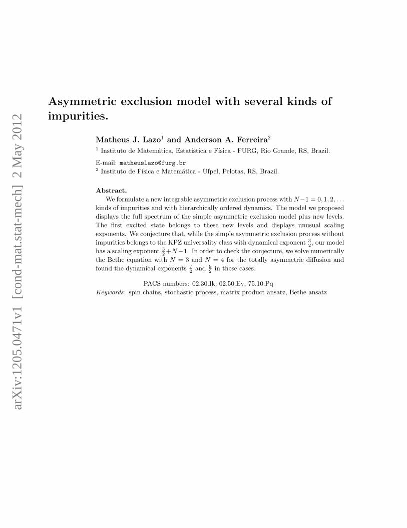
L (see Figure (1) for the cases where Γ1 00 1 = 0.7 and Γ1 0
0 1 = 0.5). In the ASEPI, we
consider the cases where Γ1 00 1 = 0.9, 0.8, 0.7, 0.6 with L = 20, 40, 80, 160, 200, 300, 400,
and we found that the energy gap has a leading behavior of KPZ L−32 and a sub-leading
Asymmetric exclusion model with several kinds of impurities. 11
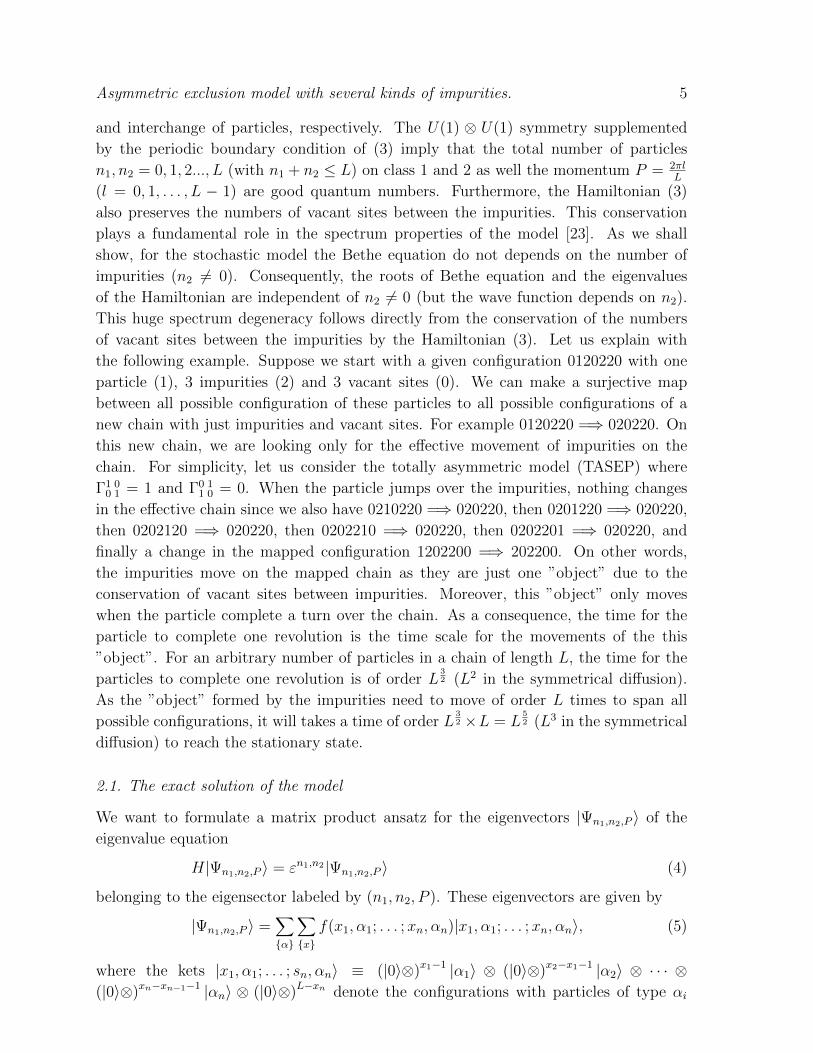
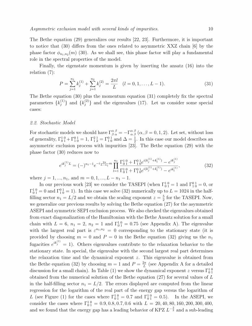
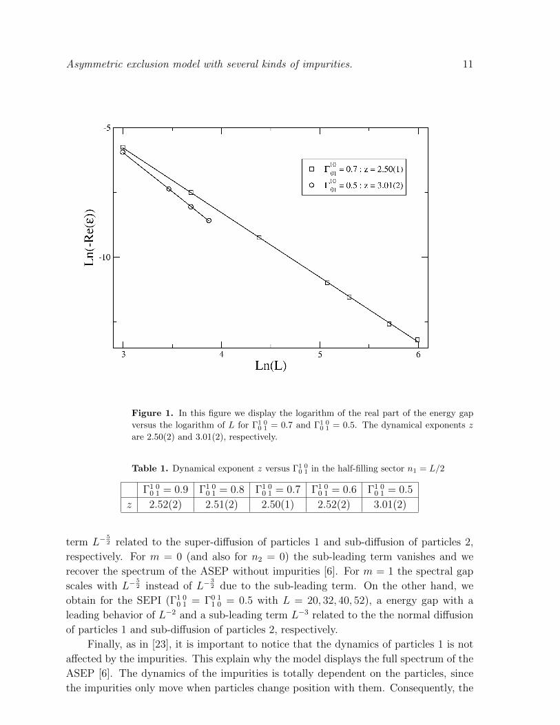
Figure 1. In this figure we display the logarithm of the real part of the energy gap
versus the logarithm of L for Γ1 00 1 = 0.7 and Γ1 0
0 1 = 0.5. The dynamical exponents z
are 2.50(2) and 3.01(2), respectively.
Table 1. Dynamical exponent z versus Γ1 00 1 in the half-filling sector n1 = L/2
Γ1 00 1 = 0.9 Γ1 0
0 1 = 0.8 Γ1 00 1 = 0.7 Γ1 0
0 1 = 0.6 Γ1 00 1 = 0.5
z 2.52(2) 2.51(2) 2.50(1) 2.52(2) 3.01(2)
term L−52 related to the super-diffusion of particles 1 and sub-diffusion of particles 2,
respectively. For m = 0 (and also for n2 = 0) the sub-leading term vanishes and we
recover the spectrum of the ASEP without impurities [6]. For m = 1 the spectral gap
scales with L−52 instead of L−
32 due to the sub-leading term. On the other hand, we
obtain for the SEPI (Γ1 00 1 = Γ0 1
1 0 = 0.5 with L = 20, 32, 40, 52), a energy gap with a
leading behavior of L−2 and a sub-leading term L−3 related to the the normal diffusion
of particles 1 and sub-diffusion of particles 2, respectively.
Finally, as in [23], it is important to notice that the dynamics of particles 1 is not
affected by the impurities. This explain why the model displays the full spectrum of the
ASEP [6]. The dynamics of the impurities is totally dependent on the particles, since
the impurities only move when particles change position with them. Consequently, the
Asymmetric exclusion model with several kinds of impurities. 12
time to vanish the fluctuations on the densities of particles acts as a time scale for the
diffusion of the impurities, resulting in a relaxation time greater than the one for the
standard ASEP and SEP (reflected in the L−32 × L−1 = L−
52 gap for the ASEPI and
L−2 × L−1 = L−3 gap for the SEPI).
Eigenstates: The stationary state is the eigenstate associated to the eigenvalue
εn1,n2 = 0 (it is in the sector with m = 0 and P = 0). In this case, the Bethe equation
(32) has the unique solution ek(α)j = 1 for all α = 1, 2 and j = 1, ..., nα. As a consequence,
the S-matrix reduces to the identity Sα1 α2α1 α2
(k(α1)j , k
(α2)l ) = 1, and all amplitudes in the
eigenfunction (5) becomes equals to a normalization constant f(x1, α1; . . . ;xn, αn) = f0,
since we have from (6) and (16):
Ex1A(α1)
kα11Ex2−x1A
(α2)
kα22· · ·Exn−xn−1A
(αn)kαnn
EL−xn (33)
= A(1)
k(1)1
· · ·A(1)
k(1)n1
A(2)
k(2)1
· · ·A(2)
k(2)n2
EL.
The eigenfunction |Ψ0〉 corresponding to the stationary state is given by a simple
combination of all possible configurations of particles, where each particle configuration
has the same weight given by the normalization constant f0. We have from (5):
|Ψ0〉 = f0
∑{α}
∑{x}|x1, α1; . . . ;xn, αn〉. (34)
Consequently, at the stationary state, all configurations that satisfy the hard-core
constraints imposed by the definition of the model occur with equal probabilities given
by f0. Furthermore, in this case each site is occupied by a particle α with probability
ρα = nα/L.
Finally, the MPA (6) enable us to write all eigenstates of (3) in a matrix product
form. For a given solution k(1)j and k
(2)j , the matrices E and A
(α)
k(α)j
have the following
finite-dimensional representation:
E =n1⊗l=1
1 0
0 eik(1)l
n2⊗l=1
1 0
0 eik(2)l
, (35)
A(2)
k(2)j
=n1⊗l=1
1 0
0Γ2 11 2
Γ0 11 0eik
(2)l
j−1⊗l=1
I2
⊗(0 0
1 0
)n2⊗
l=j+1
I2,
A(1)
k(1)j
=j−1⊗l=1
(S1 1
1 1(k(1)j , k
(1)l ) 0
0 1
)⊗(0 0
1 0
)n1+n2⊗j=j+1
I2,
where n = n1+n2, I2 is the 2×2 identity matrix, and the dimension of the representation
is 2n. The matrix product form of the eigenstates are given by inserting the matrices
(16) defining the MPA (6) with the spectral parameters (29) into equation (5). As
showed in [27], our MPA generalizes the steady-state Matrix Product introduced by
Derrida et al [28]. For the stochastic model the stationary state is obtained by choosing
k(1)j = 0 and k
(2)j = 0 in (35). However, a relation between our matrix product form for
the steady-state and the standard Matrix Product form for open boundary condition is
not trivial [27, 28].
Asymmetric exclusion model with several kinds of impurities. 13
2.3. Quantum model
We consider here only the simplest case of free fermions, when ∆ = 0 and Γ2 11 2 =
Γ1 00 1 = Γ0 1
1 0 = 1, in this particular case, the Bethe equation (29) reduces to roots of unit.
The simplicity of Bethe equation enable us to calculate analytically the eigenvalues by
following [6]. As in the stochastic model, the ground state is obtained by choosing m = 0
and the first excited state is given by m = 1. Due to the L−1 term in the phase factor,
the energy gap
∆ε =4απ
(1− ρ1)2sin
(απρ1
2
)1
L3+ O(L−4), (36)
with α = 1(2) for n1 even (odd), scales with L−3 instead of L−1 for the case of only
one kind of particle. The boundary condition plays a fundamental role in the scaling
behavior of the model. In the quantum sector our model is related to the strong regime
of the t-U Hubbard model introduced in [26] and solved with diagonal open boundary
condition. Although the open chain t-U Hubbard model has a scaling gap of L−1, since
its spectrum coincides with the spectrum of the anisotropic XXZ model [26] at ∆ = 0,
our model with periodic boundary condition displays a scaling gap of L−3.
3. The asymmetric exclusion model with N − 1 kinds of impurities
We generalize the model discussed in the previous section by adding more types of
impurities. Although we can formulate a general model including both stochastic
process and quantum spin chains, we will consider for simplicity only stochastic process.
The model introduced describes the dynamics of N types of particles on an one-
dimensional lattice of L sites, where the total number n1, n2, ..., nN of particles of
each type is conserved. Different from the case with just one kind of impurity [23],
discussed in the previous section, in our generalized model we can have more than one
particle on each site (multiple site occupation). In order to describe the occupancy
of a given site i (i = 1, 2, ..., L) we attach on site i a set {α}i = {α1, ..., αn}, where
αj = 1, ..., N (j = 1, ..., n) denotes a particle of kind αj. If {α}i = ∅, the site is
vacant. If {α}i = {α1, ..., αn}, we have on the site n particles of kinds α1, α2,...,
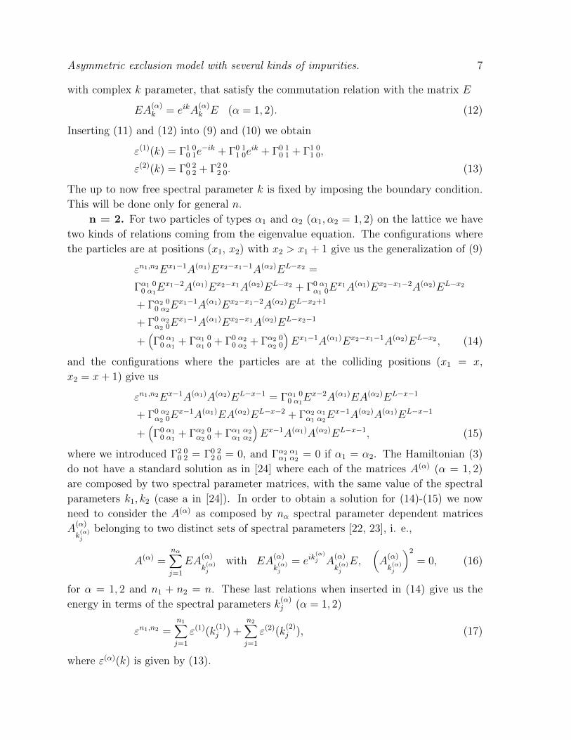
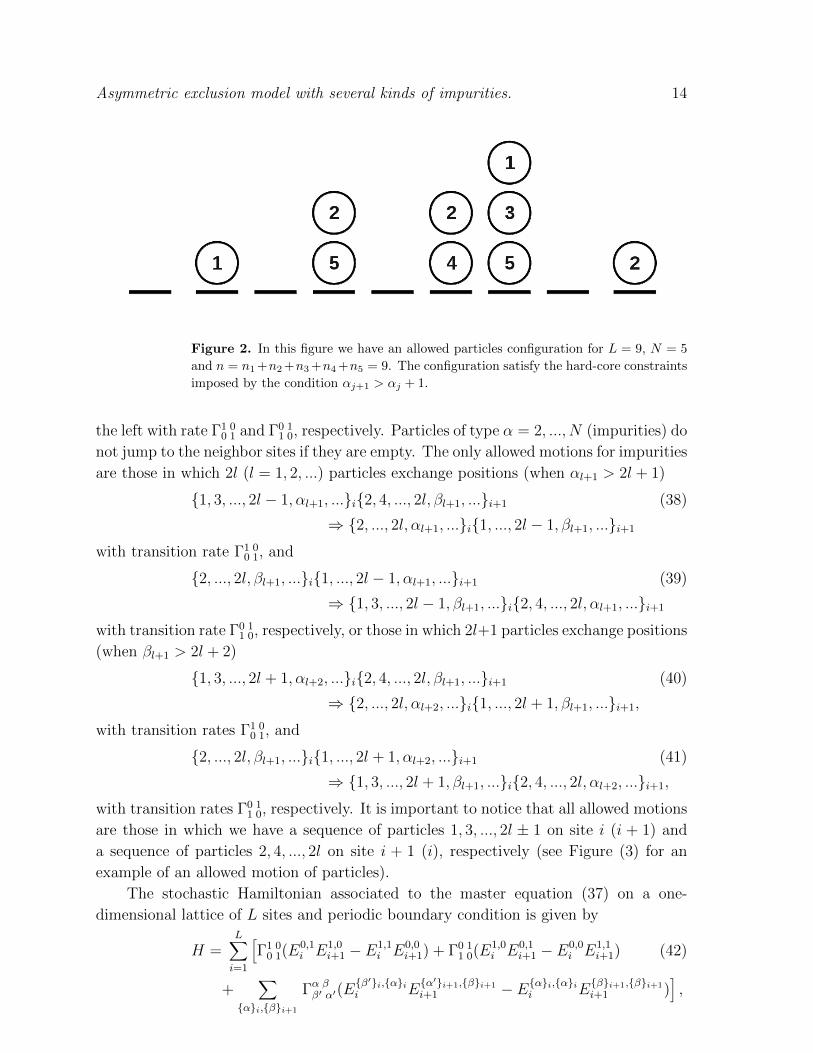
αn with αj+1 > αj + 1 (j = 1, ..., n − 1). The allowed configurations, denoted by
{α} = {{α}1, {α}2, ..., {α}L} are those satisfying the hard-core constraints imposed by
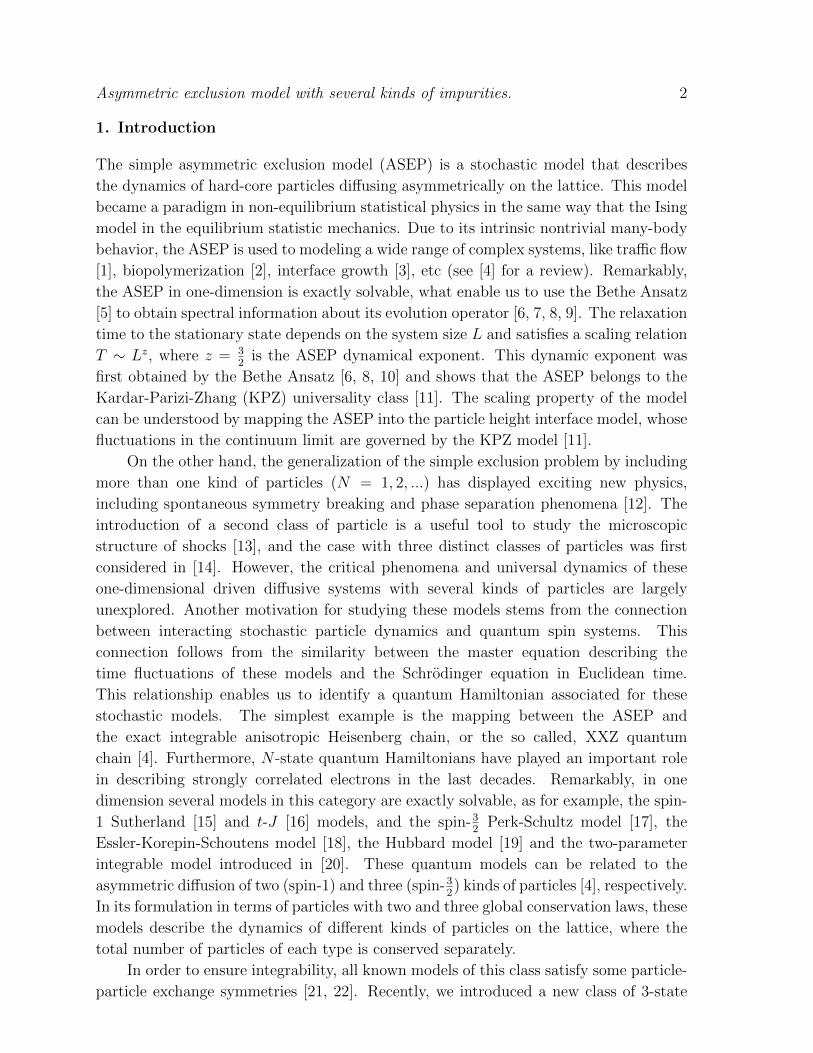
the condition αj+1 > αj + 1 for particles on the same site (see Figure (2) for an example
of an allowed configuration).
The master equation for the probability distribution at a given time t, P ({α}, t),can be written in general as
∂P ({α}, t)∂t
= −Γ({α} → {α′})P ({α}, t) + Γ({α′} → {α})P ({α′}, t) (37)
where Γ({α} → {α′}) is the transition rate where a configuration {α} changes to {α′}.In the model proposed there are only diffusion processes. As in [23], and in the last
section, if the neighbor sites are empty, particles of type α = 1 can jump to the right or to
Asymmetric exclusion model with several kinds of impurities. 14
Figure 2. In this figure we have an allowed particles configuration for L = 9, N = 5
and n = n1+n2+n3+n4+n5 = 9. The configuration satisfy the hard-core constraints
imposed by the condition αj+1 > αj + 1.
the left with rate Γ1 00 1 and Γ0 1
1 0, respectively. Particles of type α = 2, ..., N (impurities) do
not jump to the neighbor sites if they are empty. The only allowed motions for impurities
are those in which 2l (l = 1, 2, ...) particles exchange positions (when αl+1 > 2l + 1)
{1, 3, ..., 2l − 1, αl+1, ...}i{2, 4, ..., 2l, βl+1, ...}i+1 (38)
⇒ {2, ..., 2l, αl+1, ...}i{1, ..., 2l − 1, βl+1, ...}i+1
with transition rate Γ1 00 1, and
{2, ..., 2l, βl+1, ...}i{1, ..., 2l − 1, αl+1, ...}i+1 (39)
⇒ {1, 3, ..., 2l − 1, βl+1, ...}i{2, 4, ..., 2l, αl+1, ...}i+1
with transition rate Γ0 11 0, respectively, or those in which 2l+1 particles exchange positions
(when βl+1 > 2l + 2)
{1, 3, ..., 2l + 1, αl+2, ...}i{2, 4, ..., 2l, βl+1, ...}i+1 (40)
⇒ {2, ..., 2l, αl+2, ...}i{1, ..., 2l + 1, βl+1, ...}i+1,
with transition rates Γ1 00 1, and
{2, ..., 2l, βl+1, ...}i{1, ..., 2l + 1, αl+2, ...}i+1 (41)
⇒ {1, 3, ..., 2l + 1, βl+1, ...}i{2, 4, ..., 2l, αl+2, ...}i+1,
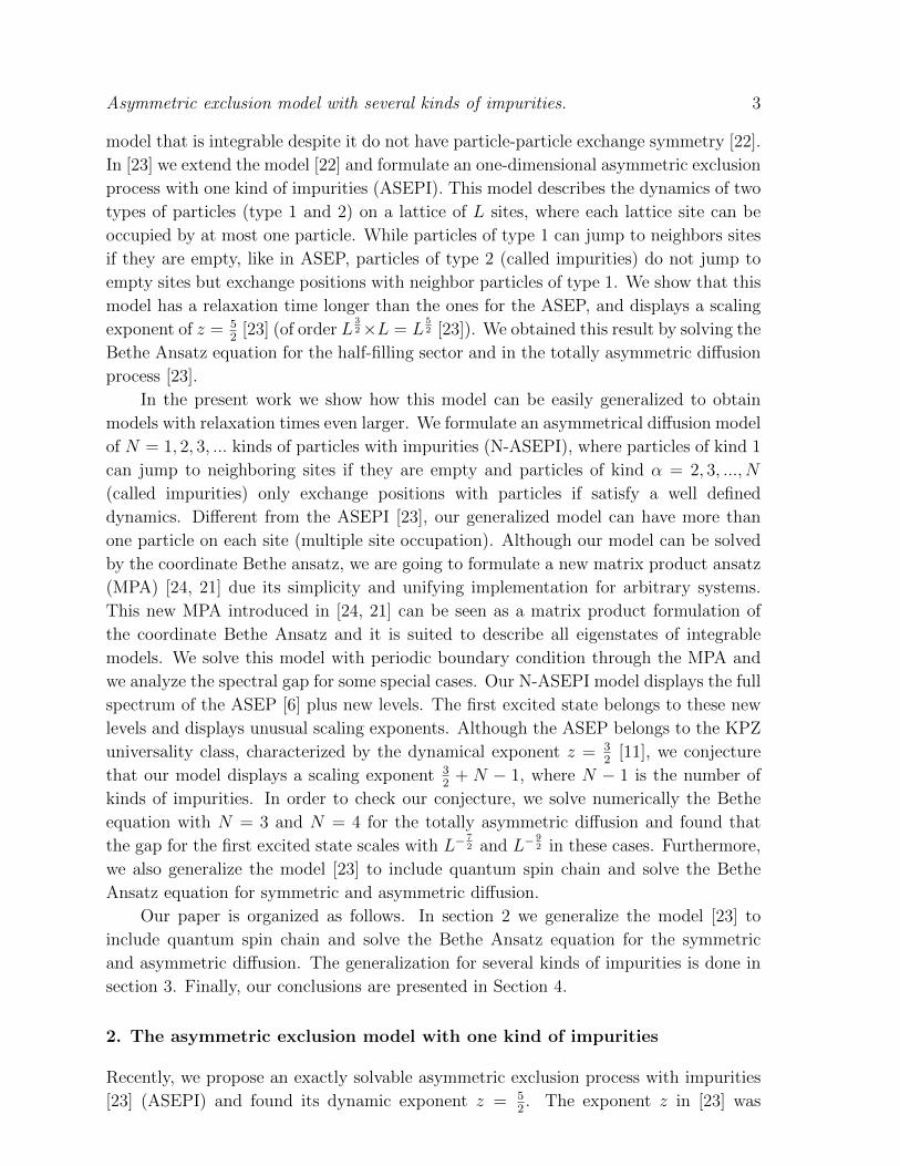
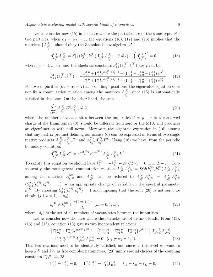
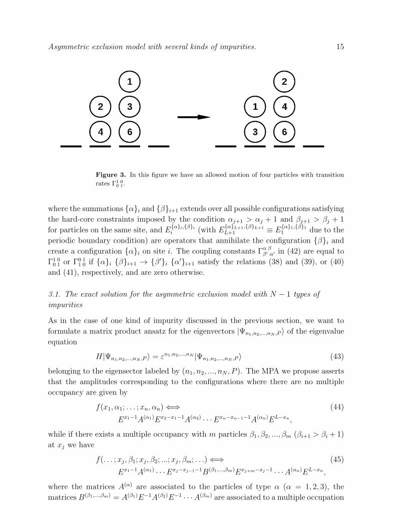
with transition rates Γ0 11 0, respectively. It is important to notice that all allowed motions
are those in which we have a sequence of particles 1, 3, ..., 2l ± 1 on site i (i + 1) and
a sequence of particles 2, 4, ..., 2l on site i + 1 (i), respectively (see Figure (3) for an
example of an allowed motion of particles).
The stochastic Hamiltonian associated to the master equation (37) on a one-
dimensional lattice of L sites and periodic boundary condition is given by
H =L∑i=1
[Γ1 0
0 1(E0,1i E1,0
i+1 − E1,1i E0,0
i+1) + Γ0 11 0(E1,0
i E0,1i+1 − E
0,0i E1,1
i+1) (42)
+∑
{α}i,{β}i+1
Γα ββ′ α′(E{β′}i,{α}ii E
{α′}i+1,{β}i+1
i+1 − E{α}i,{α}ii E{β}i+1,{β}i+1
i+1 )],
Asymmetric exclusion model with several kinds of impurities. 15
Figure 3. In this figure we have an allowed motion of four particles with transition
rates Γ1 00 1.
where the summations {α}i and {β}i+1 extends over all possible configurations satisfying
the hard-core constraints imposed by the condition αj+1 > αj + 1 and βj+1 > βj + 1
for particles on the same site, and E{α}i,{β}ii (with E
{α}L+1,{β}L+1
L+1 ≡ E{α}1,{β}11 due to the
periodic boundary condition) are operators that annihilate the configuration {β}i and
create a configuration {α}i on site i. The coupling constants Γα ββ′ α′ in (42) are equal to
Γ1 00 1 or Γ0 1
1 0 if {α}i {β}i+1 → {β′}i {α′}i+1 satisfy the relations (38) and (39), or (40)
and (41), respectively, and are zero otherwise.
3.1. The exact solution for the asymmetric exclusion model with N − 1 types of
impurities
As in the case of one kind of impurity discussed in the previous section, we want to
formulate a matrix product ansatz for the eigenvectors |Ψn1,n2,...,nN ,P 〉 of the eigenvalue
equation
H|Ψn1,n2,...,nN ,P 〉 = εn1,n2,...,nN |Ψn1,n2,...,nN ,P 〉 (43)
belonging to the eigensector labeled by (n1, n2, ..., nN , P ). The MPA we propose asserts
that the amplitudes corresponding to the configurations where there are no multiple
occupancy are given by
f(x1, α1; . . . ;xn, αn)⇐⇒ (44)
Ex1−1A(α1)Ex2−x1−1A(α2) · · ·Exn−xn−1−1A(αn)EL−xn ,
while if there exists a multiple occupancy with m particles β1, β2, ..., βm (βi+1 > βi + 1)
at xj we have
f(. . . ;xj, β1;xj, β2; ...;xj, βm; . . .)⇐⇒ (45)
Ex1−1A(α1) · · ·Exj−xj−1−1B(β1,...,βm)Exj+m−xj−1 · · ·A(αn)EL−xn ,
where the matrices A(α) are associated to the particles of type α (α = 1, 2, 3), the
matrices B(β1,...,βm) = A(β1)E−1A(β2)E−1 · · ·A(βm) are associated to a multiple occupation
Asymmetric exclusion model with several kinds of impurities. 16
of m particles β1, β2, ..., βm at same site, and the matrix E is associated to vacant sites.
Furthermore, as the Hamiltonian (42) commutes with the momentum operator due to
the periodic boundary condition, the amplitudes f(x1, α1; . . . ;xn, αn) should satisfy the
following relations:
f(x1, α1; . . . ;xn, αn) = e−iPf(x1 + 1, α1; . . . ;xn + 1, αn), (46)
where
P =2πl
L, l = 0, 1, ..., L− 1. (47)
The eigenvalue equation (43) give us two kinds of relations for the amplitudes (44)
and (45). The first kind is related to those amplitudes without multiple occupancy, and
the second type is related to those amplitudes with multiple occupancy. Let us consider
separated each case:
Without multiple occupancy: In this case, we have from the eigenvalue equation
(43) relations for amplitudes without collisions (particles of kind 1 have only empty
neighboring sites) and with collisions. For configuration without collision the amplitudes
should satisfy the following constraints:
εn1,n2,...,nNf(x1, α1; ...;xn, αn) (48)
=n∑i=1
[Γαi 0
0 αif(...;xi − 1, αi; ...) + Γ0 αiαi 0f(...;xi + 1, αi; ...)
]− n1f(x1, α1; ...;xn, αn),
where we introduced Γ0 αα 0 = Γα 0
0 α = 0 for α 6= 1. In order to obtain a solution for
(48) we need to generalize (16) for N kinds of particles. We consider the matrices A(α)
(α = 1, ..., N) as composed by nα spectral parameter dependent matrices A(α)
k(α)j
belonging
to N distinct sets of spectral parameters, i. e.,
A(α) =nα∑j=1
EA(α)
k(α)j
with EA(α)
k(α)j
= eik(α)j A
(α)
k(α)j
E,(A
(α)
k(α)j
)2
= 0, (49)
for α = 1, 2, ..., N and n1 + n2 + · · · + nN = n. These expressions when inserted into
relations without collisions (48) give us the energy in terms of the spectral parameters
{k(1)j }
εn1,n2,...,nN =n1∑j=1
ε(k(1)j ), (50)
where
ε(k) = Γ1 00 1e−ik + Γ0 1
1 0eik − 1. (51)
It is important to notice that, like in the previous section, the eigenvalues of the model
depend only on the spectral parameters of particles of kind 1. On the other hand, for
amplitudes without multiple occupancy and particles of kind α and β at the colliding
Asymmetric exclusion model with several kinds of impurities. 17
positions (xj+1 = xj + 1), the eigenvalue equation (43) give us the generalizations of
(26) with α, β = 1, 2, where the S-matrix elements are given by
S1 11 1(k
(1)j , k
(1)l ) = − Γ1 0
0 1 + Γ0 11 0e
i(k(1)j +k
(1)l
) − eik(1)j
Γ1 00 1 + Γ0 1
1 0ei(k
(1)j +k
(1)l
) − eik(1)l
, (52)
S2 12 1(k(2), k(1)) =
1
S1 21 2(k(1), k(2))
= eik(2)
.
We do not consider here the cases where we have one particle of kind 1 and other particle
of kind greater than 2 since the eigenvalue equation in this case will relates amplitudes
with multiple occupancy. For α, β ≥ 2 the relations coming from the eigenvalue equation
are identically satisfied. In this case, as in the previous section, we can choose without
loss of generality
Sα αα α(k(α)j , k
(α)l ) = 1 (α ≥ 2). (53)
Furthermore, in order to have amplitudes with non null norm, the spectral parameters
{k(α)j } (α ≥ 2) should satisfy the constraints
k(α)l 6= k
(α)j +
π(2m+ 1)
d(α)v
(m = 0, 1, ...) (α ≥ 2), (54)
where {d(α)v } is the set of all numbers of vacant sites between particles of type α ≥ 2.
With multiple occupancy: Let us consider first the relations coming from the
eigenvalue equation (43) where we have only one site with multiple occupancy of m
particles β1, β2, ..., βm (βi+1 > βi + 1) at position xj ≡ x. We have from the eigenvalue
equation (43) the following relations:
εn1,n2,...,nNf(...;x, β1;x, β2; ...;x, βm; ...) (55)
=n∑
i=1,xi 6=x
[Γαi 0
0 αif(...;xi − 1, αi; ...) + Γ0 αiαi 0f(...;xi + 1, αi; ...)
]+ Γβ1 0
0 β1f(...;x− 1, β1;x, β2; ..., x, βm; ...)
+ Γ0 β1β1 0f(...;x, β2; ..., x, βm;x+ 1, β1; ...)
− n1f(...;x, β1;x, β2; ...;x, βm; ...),
for empty neighboring sites, and
εn1,n2,...,nNf(...;x− 1, β1;x, β2; ...;x, βm; ...) (56)
=n∑
i=1,xi 6=x−1,x
[Γαi 0
0 αif(...;xi − 1, αi; ...) + Γ0 αiαi 0f(...;xi + 1, αi; ...)
]+ Γβ1 0
0 β1f(...;x− 2, β1;x, β2; ..., x, βm; ...)
+ Γ0 β1β1 0f(...;x, β1;x, β2; ..., x, βm; ...)
− n1f(...;x, β1;x, β2; ...;x, βm; ...),
and
εn1,n2,...,nNf(...;x, β2; ...;x, βm;x+ 1, β1...) (57)
Asymmetric exclusion model with several kinds of impurities. 18
=n∑
i=1,xi 6=x,x+1
[Γαi 0
0 αif(...;xi − 1, αi; ...) + Γ0 αiαi 0f(...;xi + 1, αi; ...)
]+ Γβ1 0
0 β1f(...;x, β1;x, β2; ..., x, βm; ...)
+ Γ0 β1β1 0f(...;x, β2; ..., x, βm;x+ 2, β1; ...)
− n1f(...;x, β1;x, β2; ...;x, βm; ...),
for neighboring sites occupied by one particle of kind β1. In (55), (56) and (57) we
have β1 = 1, 2, ..., N and Γβ1 00 β1
= Γ0 β1β1 0 = 0 if β1 6= 1, and without loss of generality we
also choose no collisions of particles 1. Equations (55), (56) and (57) are automatically
satisfied if β1 6= 1. On the other hand, for β1 = 1, while (56) is again automatically
satisfied, the equations (55) and (57) will impose algebraic constraints for the matrices
defining the ansatz. By inserting the ansatz (45) with (49) and (50) into equations (55)
and (57) we obtain, after some algebraic manipulations, the following constraints among
the matrices:
A(1)
k(1)A
(β2)
k(β2)· · ·A(βm)
k(βm) = A(β2)
k(β2)· · ·A(βm)
k(βm)A(1)
k(1), (58)
where β2 = 3, 4, ..., N and m = 2, 3, ... with βi+1 > βi + 1. In order to satisfy (58) the
for any set {β2, ..., βm} we should impose the following commutation relations among
matrices A(1)
k(1)j
and A(α)
k(α)j
(α ≥ 3):
A(1)
k(1)j
A(α)
k(α)j
= A(α)
k(α)j
A(1)
k(1)j
(α ≥ 3). (59)
Let us consider now the configurations where we have neighbors sites at positions
x and x + 1 with multiple particle occupations. For those configurations in which
2l (l = 1, 2, ...) particles exchange positions the eigenvalue equation (43) give us the
following relations:
εn1,n2,...,nNf(...;x, 1; ...;x, 2l − 1;x, βl+1; ...;x, βm; (60)
x+ 1, 2; ...;x+ 1, 2l;x+ 1, β′l+1; ...;x+ 1, β′m′ ; ...)
=n∑
i=1,xi 6=x,x+1
[Γαi 0
0 αif(...;xi − 1, αi; ...) + Γ0 αiαi 0f(...;xi + 1, αi; ...)
]+ Γ1 0
0 1f(...;x− 1, 1;x, 3; ...;x, βm; ...)
+ Γ0 11 0f(...;x, 2; ...;x, 2l;x, βl+1; ...;x, βm;
x+ 1, 1; ...;x+ 1, 2l − 1;x+ 1, β′l+1; ...;x+ 1, β′m′ ; ...)
− n1f(...;x, 1; ...;x, 2l − 1;x, βl+1; ...;x, βm;
x+ 1, 2; ...;x+ 1, 2l;x+ 1, β′l+1; ...;x+ 1, β′m′ ; ...)
and
εn1,n2,...,nNf(...;x, 2; ...;x, 2l;x, β′l+1; ...;x, β′m′ ; (61)
x+ 1, 1; ...;x+ 1, 2l − 1;x+ 1, βl+1; ...;x+ 1, βm; ...)
=n∑
i=1,xi 6=x,x+1
[Γαi 0
0 αif(...;xi − 1, αi; ...) + Γ0 αiαi 0f(...;xi + 1, αi; ...)
]
Asymmetric exclusion model with several kinds of impurities. 19
+ Γ0 11 0f(...;x+ 1, 3; ...;x+ 1, β′m′ ;x+ 2, 1; ...)
+ Γ1 00 1f(...;x, 1; ...;x, 2l − 1;x, β′l+1; ...;x, β′m′ ;
x+ 1, 2; ...;x+ 1, 2l;x+ 1, βl+1; ...;x+ 1, βm; ...)
− n1f(...;x, 2; ...;x, 2l;x, β′l+1; ...;x, β′m′ ;
x+ 1, 1; ...;x+ 1, 2l − 1;x+ 1, βl+1; ...;x+ 1, βm; ...),
where βl+1 > 2l + 1. Furthermore, for those configurations in which 2l + 1 (l = 0, 1, ...)
particles exchange positions the eigenvalue equation (43) give us
εn1,n2,...,nNf(...;x, 1; ...;x, 2l + 1;x, βl+2; ...;x, βm; (62)
x+ 1, 2; ...;x+ 1, 2l;x+ 1, β′l+1; ...;x+ 1, β′m′ ; ...)
=n∑
i=1,xi 6=x,x+1
[Γαi 0
0 αif(...;xi − 1, αi; ...) + Γ0 αiαi 0f(...;xi + 1, αi; ...)
]+ Γ1 0
0 1f(...;x− 1, 1;x, 3; ...;x, βm; ...)
+ Γ0 11 0f(...;x, 2; ...;x, 2l;x, βl+2; ...;x, βm;
x+ 1, 1; ...;x+ 1, 2l + 1;x+ 1, β′l+1; ...;x+ 1, β′m′ ; ...)
− n1f(...;x, 1; ...;x, 2l + 1;x, βl+2; ...;x, βm;
x+ 1, 2; ...;x+ 1, 2l;x+ 1, β′l+1; ...;x+ 1, β′m′ ; ...)
and
εn1,n2,...,nNf(...;x, 2; ...;x, 2l;x, β′l+1; ...;x, β′m′ ; (63)
x+ 1, 1; ...;x+ 1, 2l + 1;x+ 1, βl+2; ...;x+ 1, βm; ...)
=n∑
i=1,xi 6=x,x+1
[Γαi 0
0 αif(...;xi − 1, αi; ...) + Γ0 αiαi 0f(...;xi + 1, αi; ...)
]+ Γ0 1
1 0f(...;x+ 1, 3; ...;x+ 1, βm;x+ 2, 1; ...)
+ Γ1 00 1f(...;x, 1; ...;x, 2l + 1;x, β′l+1; ...;x, β′m′ ;
x+ 1, 2; ...;x+ 1, 2l;x+ 1, βl+2; ...;x+ 1, βm; ...)
− n1f(...;x, 2; ...;x, 2l;x, β′l+1; ...;x, β′m′ ;
x+ 1, 1; ...;x+ 1, 2l + 1;x+ 1, βl+2; ...;x+ 1, βm; ...),
where β′l+1 > 2l+2. By inserting the ansatz (45) with (49), (50) and (59) into equations
(60)-(63) we obtain, after some algebraic manipulations, the following constraints among
the matrices:
ei(k(2)+···+k(2l))A
(1)
k(1)· · ·A(2l−1)
k(2l−1)A(βl+1)
k(βl+1)· · ·A(βm)
k(βm)A(2)
k(2)· · ·A(2l)
k(2l)= (64)
ei(k(3)+···+k(2l−1))A
(2)
k(2)· · ·A(2l)
k(2l)A
(βl+1)
k(βl+1)· · ·A(βm)
k(βm)A(1)
k(1)· · ·A(2l−1)
k(2l−1) ,
and
ei(k(2)+···+k(2l))A
(1)
k(1)· · ·A(2l+1)
k(2l+1)A(βl+1)
k(βl+1)· · ·A(βm)
k(βm)A(2)
k(2)· · ·A(2l)
k(2l)= (65)
ei(k(3)+···+k(2l+1))A
(2)
k(2)· · ·A(2l)
k(2l)A
(βl+1)
k(βl+1)· · ·A(βm)
k(βm)A(1)
k(1)· · ·A(2l+1)
k(2l+1) .
Asymmetric exclusion model with several kinds of impurities. 20
In order to satisfy equations (64) and (65) for all l = 0, 1, ... and m = 2, 3, ... with
βi+1 > βi + 1, the matrices defining the ansatz should satisfy the algebraic relations:
A(α+1)
k(α+1)A(α)
k(α)= eik
(α+1)
A(α)
k(α)A
(α+1)
k(α+1) (α = 1, ..., N − 1) (66)
A(α)
k(α)A
(β)
k(β)= A
(β)
k(β)A
(α)
k(α)(β > α + 1).
Equations (66) with (49), (52), (53) and (59) completely fix the commutation relations
among the matrices defining the ansatz:
EA(α)
k(α)j
= eik(α)j A
(α)
k(α)j
E,(A
(α)
k(α)j
)2
= 0, (67)
A(α)
k(α)j
A(β)
k(β)l
= Sα βα β (k(α)j , k
(β)l )A
(β)
k(β)l
A(α)
k(α)j
(α, β = 1, 2, ..., N),
where the coupling constants Sα βα β (k(α)j , k
(β)l ) are given by:
S1 11 1(k
(1)j , k
(1)l ) = −Γ1 0
0 1 + Γ0 11 0e
i(k(1)j +k
(1)l
) − eik(1)j
Γ1 00 1 + Γ0 1
1 0ei(k
(1)j +k
(1)l
) − eik(1)l
, (68)
Sα αα α(k(α)j , k
(α)l ) = 1 (2 ≤ α ≤ N),
Sα+1 αα+1 α(k
(α+1)j , k
(α)l ) =
1
Sα α+1α α+1(k
(α)l , k
(α+1)j )
= eik(α+1)j (1 ≤ α ≤ N − 1),
Sα βα β (k(α)j , k
(β)l ) = Sβ αβ α(k
(β)l , k
(α)j ) = 1 (α = 1, ..., N − 1, α + 1 < β ≤ N).
Finally, all other relations coming from the eigenvalue equation (43) containing
amplitudes with arbitrary number of particles on neighbors sites are automatically
satisfied by the ansatz (44) and (45) with (49) and the algebraic relations (67).
Furthermore, the associativity of the algebra (67) provides a well-defined value
for any product of matrices and it follows from the fact that the algebra (67)
is diagonal and the structure constants (68) are c-numbers with the property
Sα βα β (k(α)j , k
(β)l )Sβ αβ α(k
(β)l , k
(α)j ) = 1 (α, β = 1, ..., N).
In order to complete our solution we should fix the spectral parameters {k(α)j }
(α = 1, ..., N). Like in previous section, the algebraic expression in (67) assures that
any matrix product defining our ansatz can be expressed in terms of a simple matrix
product A(1)
k(1)1
· · ·A(1)
k(1)n1
A(2)
k(2)1
· · ·A(2)
k(2)n2
· · ·A(N)
k(N)1
· · ·A(N)
k(N)nN
EL. From the periodic boundary
condition we obtain:
A(1)
k(1)1
· · ·A(1)
k(1)j−1
A(1)
k(1)j
A(1)
k(1)j+1
· · ·A(N)
k(N)nN
EL (69)
=n1∏l>j
S1 11 1(k
(1)j , k
(1)l )e−i
∑n2q=1
k(2)q e−ik
(1)j LA
(1)
k(1)1
· · ·A(1)
k(1)j−1
A(1)
k(1)j+1
· · ·A(N)
k(N)nN
ELA(1)
k(1)j
=n1∏l>j
S1 11 1(k
(1)j , k
(1)l )e−i
∑n2q=1
k(2)q e−ik
(1)j LA
(1)
k(1)j
A(1)
k(1)1
· · ·A(1)
k(1)j−1
A(1)
k(1)j+1
· · ·A(N)
k(N)nN
EL
= −n1∏l=1
S1 11 1(k
(1)j , k
(1)l )e−i
∑n2q=1
k(2)q e−ik
(1)j L
×A(1)
k(1)1
· · ·A(1)
k(1)j−1
A(1)
k(1)j
A(1)
k(1)j+1
· · ·A(N)
k(N)nN
EL,
Asymmetric exclusion model with several kinds of impurities. 21
and
A(1)
k(1)1
· · ·A(α)
k(α)j−1
A(α)
k(α)j
A(α)
k(α)j+1
· · ·A(N)
k(N)nN
EL (70)
= e−i∑nα+1
q=1 k(α+1)q e−ik
(α)j LA
(1)
k(1)1
· · ·A(α)
k(α)j−1
A(α)
k(α)j+1
· · ·A(N)
k(N)nN
ELA(α)
k(α)j
= e−i∑nα+1
q=1 k(α+1)q e−ik
(α)j LA
(α)
k(α)j
A(1)
k(1)1
· · ·A(α)
k(α)j−1
A(α)
k(α)j+1
· · ·A(N)
k(N)nN
EL
= e−i∑nα+1
q=1 k(α+1)q e−ik
(α)j (L−nα−1)A
(1)
k(1)1
· · ·A(α)
k(α)j−1
A(α)
k(α)j
A(α)
k(α)j+1
· · ·A(N)
k(N)nN
EL,
for α = 2, ..., N − 1, and
A(1)
k(1)1
· · ·A(N)
k(N)j−1
A(N)
k(N)j
A(N)
k(N)j+1
· · ·A(N)
k(N)nN
EL (71)
= e−ik(N)j LA
(1)
k(1)1
· · ·A(N)
k(N)j−1
A(N)
k(N)j+1
· · ·A(N)
k(N)nN
ELA(N)
k(N)j
= e−ik(N)j LA
(N)
k(N)j
A(1)
k(1)1
· · ·A(N)
k(N)j−1
A(N)
k(N)j+1
· · ·A(N)
k(N)nN
EL
= e−ik(N)j (L−nN−1)A
(1)
k(1)1
· · ·A(N)
k(N)j−1
A(N)
k(N)j
A(N)
k(N)j+1
· · ·A(N)
k(N)nN
EL,
where in (69), (69) and (71) we used the algebraic relations (67) with (68) and we
introduced S1 11 1(k
(1)j , k
(1)j ) = −1. From (69), (69) and (71) we obtain the Bethe equations
for our model:
eik(1)j L = (−)n1−1e−i
∑n2q=1
k(2)q
n1∏l=1
Γ1 00 1 + Γ0 1
1 0ei(k
(1)j +k
(1)l
) − eik(1)j
Γ1 00 1 + Γ0 1
1 0ei(k
(1)j +k
(1)l
) − eik(1)l
, (72)
eik(α)j (L−nα−1) = e−i
∑nα+1q=1 k
(α+1)q (α = 2, ..., N − 1), (73)
eik(N)j (L−nN−1) = 1, (74)
where equations should be satisfied for all k(α)j (α = 1, ..., N) with j = 1, ..., nα. On the
other hand, the momentum of the eigenstate is given by inserting the ansatz (44) and
(45) into relation (46) and (47):
P =n1∑j=1
k(1)j +
n2∑j=1
k(2)j + · · ·+
nN∑j=1
k(N)j =
2πl
L(l = 0, 1, . . . , L− 1). (75)
where the spectral parameters satisfy the Bethe equation (72), (73) and (74).
The Bethe equations (72), (73) and (74) are more complicated than the case of
previous section since the spectral parameters, and the eigenvalues of our model, depend
on the densities of impurities. We compare the Bethe equation solution (78) for N = 3
with the eigenvalues obtained from direct diagonalization of the Hamiltonian (42) with
L = 5, n1 = 2, n2 = 1 and n3 = 1 (see Appendix B). The model displays the full
spectrum of the ASEP and additional eigenvalues. The spectrum of the ASEP is
obtained when∑nαj=1 k
(α)j = 0 for all α = 2, ..., N . The stationary state belongs to
this case and has the eigenvalue with the largest real part εn1,n2 = 0. In order to obtain
the second largest real part eigenvalue, we can rewritten the Bethe equations in a more
Asymmetric exclusion model with several kinds of impurities. 22
convenient way by eliminating the the spectral parameters k(2)j in equation (72). The
first excited state is obtained when we havenα∑j=1
k(α)j =
2π
(L− nN−1)(L− nN−2) · · · (L− nα−1)(76)
for all α = 2, ..., N (see Appendix B for a detailed discussion for a small system). Hence,
by using (76) we can relate the sum over spectral parameters k(2)j for the first excited
state with roots of unity:n2∑q=1
k(2)q =
2π
LN−1
N−1∏l=1
(1− ρl)−1, (77)
where ρl = nlL
are the densities of particles of kind l = 1, ..., N . Finally, inserting (77)
into (72) we obtain the following Bethe equation:
eik(1)j L = (−)n1−1e−i
2π
LN−1
∏N−1
l=1(1−ρl)−1
n1∏l=1
Γ1 00 1 + Γ0 1
1 0ei(k
(1)j +k
(1)l
) − eik(1)j
Γ1 00 1 + Γ0 1
1 0ei(k
(1)j +k
(1)l
) − eik(1)l
. (78)
The Bethe equation (78) generalizes [22, 23] and (29) to the case of N − 1 kinds of
impurities. As in the case of one kind of impurities (N = 2), the phase factor on (78)
plays a fundamental role in the spectral properties of the model. The eigenvalue with
the second largest real part determines the relaxation time and the dynamical exponent
z. This eigenvalue is provided by selecting n1 fugacities from (78) with momentum
P = 2πL
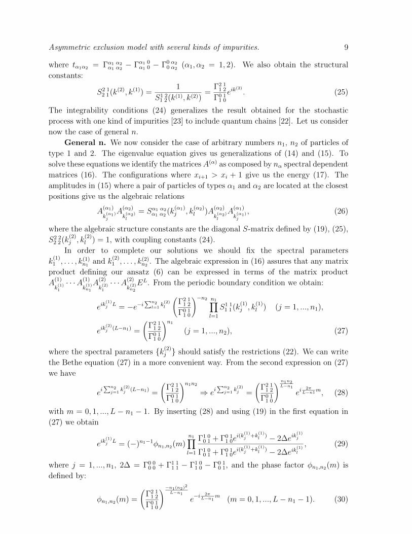
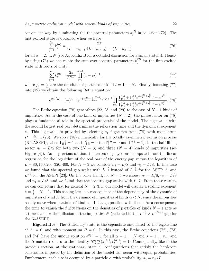
in (75). We solve (78) numerically for the totally asymmetric exclusion process
(N-TASEPI), when Γ1 00 1 = 1 and Γ0 1
1 0 = 0 (or Γ1 00 1 = 0 and Γ0 1
1 0 = 1), in the half-filling
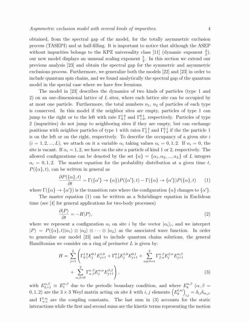
sector n1 = L/2 for both two (N = 3) and three (N = 4) kinds of impurities (see
Figure (4)). As in previous section, the errors displayed are computed from the linear
regression for the logarithm of the real part of the energy gap versus the logarithm of
L = 80, 160, 200, 320, 400. For N = 3 we consider n2 = L/8 and n3 = L/8. In this case
we found that the spectral gap scales with L−72 instead of L−
32 for the ASEP [6] and
L−52 for the ASEPI [23]. On the other hand, for N = 4 we choose n2 = L/8, n3 = L/8
and n4 = L/8, and we found that the spectral gap scales with L−92 . From these results,
we can conjecture that for general N = 2, 3, ... our model will display a scaling exponent
z = 32
+N − 1. This scaling law is a consequence of the dependency of the dynamic of
impurities of kind N from the dynamic of impurities of kinds α < N , since the impurities
α only move when particles of kind α−1 change position with them. As a consequence,
the time to vanish the fluctuations on the densities of particles of kinds N − 1 acts as
a time scale for the diffusion of the impurities N (reflected in the L−32 ×L−N+1 gap for
the N-ASEPI).
Eigenstates: The stationary state is the eigenstate associated to the eigenvalue
εn1,n2 = 0, and with momentum P = 0. In this case, the Bethe equations (72), (73)
and (74) have the unique solution ek(α)j = 1 for all α = 1, ..., N and j = 1, ..., nα, and
the S-matrix reduces to the identity Sα1 α2α1 α2
(k(α1)j , k
(α2)l ) = 1. Consequently, like in the
previous section, at the stationary state all configurations that satisfy the hard-core
constraints imposed by the definition of the model can occur with equal probabilities.
Furthermore, each site is occupied by a particle α with probability ρα = nα/L.
Asymmetric exclusion model with several kinds of impurities. 23
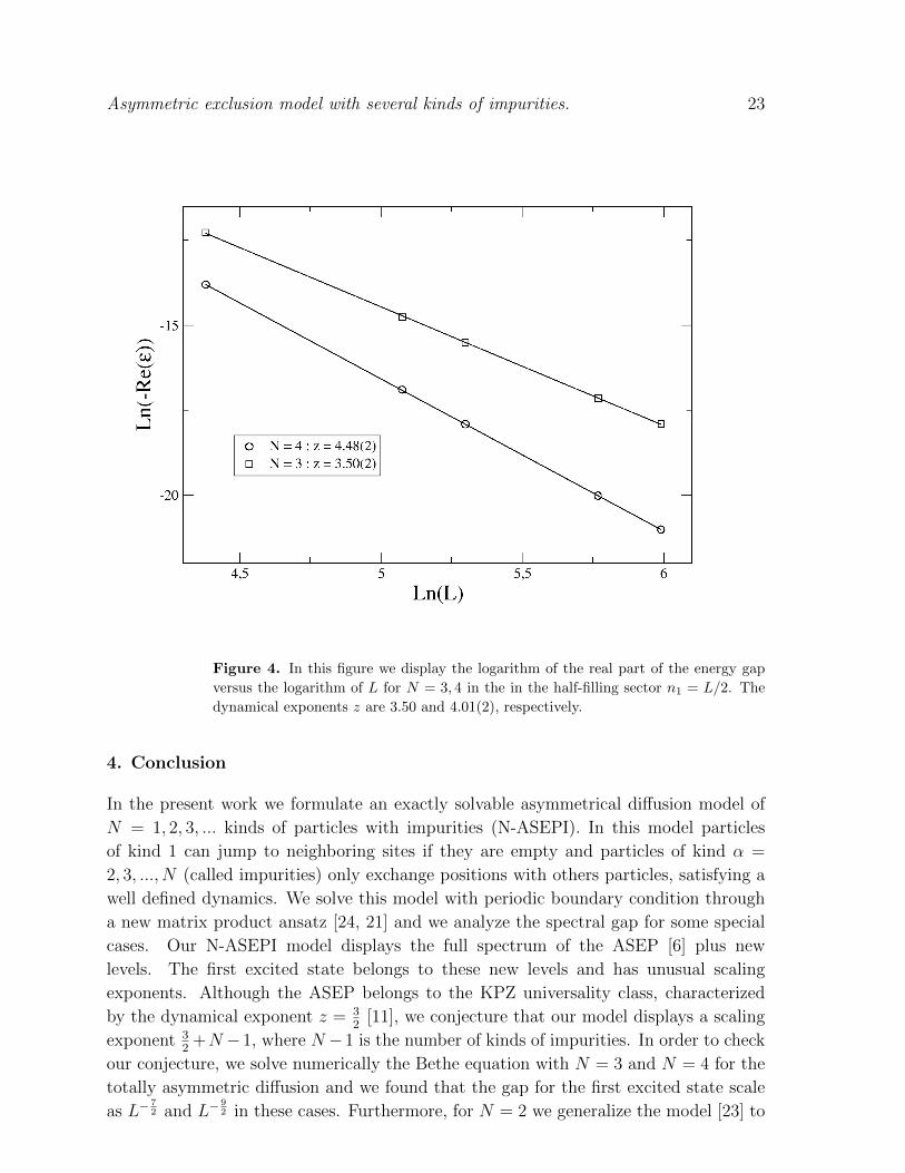
Figure 4. In this figure we display the logarithm of the real part of the energy gap
versus the logarithm of L for N = 3, 4 in the in the half-filling sector n1 = L/2. The
dynamical exponents z are 3.50 and 4.01(2), respectively.
4. Conclusion
In the present work we formulate an exactly solvable asymmetrical diffusion model of
N = 1, 2, 3, ... kinds of particles with impurities (N-ASEPI). In this model particles
of kind 1 can jump to neighboring sites if they are empty and particles of kind α =
2, 3, ..., N (called impurities) only exchange positions with others particles, satisfying a
well defined dynamics. We solve this model with periodic boundary condition through
a new matrix product ansatz [24, 21] and we analyze the spectral gap for some special
cases. Our N-ASEPI model displays the full spectrum of the ASEP [6] plus new
levels. The first excited state belongs to these new levels and has unusual scaling
exponents. Although the ASEP belongs to the KPZ universality class, characterized
by the dynamical exponent z = 32
[11], we conjecture that our model displays a scaling
exponent 32
+N −1, where N −1 is the number of kinds of impurities. In order to check
our conjecture, we solve numerically the Bethe equation with N = 3 and N = 4 for the
totally asymmetric diffusion and we found that the gap for the first excited state scale
as L−72 and L−
92 in these cases. Furthermore, for N = 2 we generalize the model [23] to
Asymmetric exclusion model with several kinds of impurities. 24
include quantum spin chain Hamiltonians and we analyze the Bethe Ansatz equation
for the symmetric and asymmetric diffusions. A quite interesting problem for the future
concerns the formulation of the model with open boundary conditions instead periodic
ones. In this case we expect the critical behavior of the model will display the same
scaling exponent 32
+N − 1.
Acknowledgments
This work has been partly supported by CNPq, CAPES and FAPERGS (Brazilian
agencies).
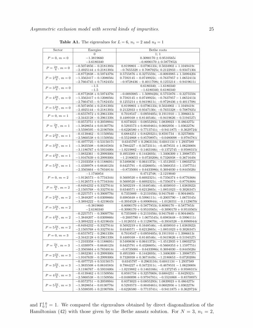
Appendix A. Eigenvalues and Bethe roots for N = 2, n1 = 2, n2 = 1, and
L = 6
In this appendix we list the full spectrum of the Hamiltonian (3) for the asymmetric
exclusion model with one kind of impurity for N = 2, n1 = 2, n2 = 1, L = 6, and
Γ1 00 1 = 0.75. We compared the eigenvalues obtained by direct diagonalization of the
Hamiltonian (3) with those given by the Bethe ansatz solution. For N = 2, n1 = 2,
n2 = 1, L = 6, and Γ1 00 1 = 0.75 the Bethe equations (32) reduces to
x6 = −e−i2π4m0.75 + 0.25xy − x
0.75 + 0.25xy − y, (A.1)
where m = 0, 1, 2, 3 and x = eik(1)1 and y = eik
(1)2 are the fugacities. Equation (A.1) can
be reduced to a simple polynomial equation by inserting the relation for the momentum
P = 2πl6
(31)
xy = ei2πl6
+i 2π4m, (A.2)
where l = 0, 1, 2, 3, 4, 5 and we have used (28). In table (A1) we display the full spectrum
of the Hamiltonian (3) and the associated Bethe roots x and y. The eigenvalue with the
largest real part is zero, it is provided by choosing m = 0 and P = 0 (l = 0) in (A.1) and
(A.2). In this case all spectral parameters are zero and we have eik(1)1 = eik
(1)2 = eik
(2)1 = 1.
It is also important to note that for m = 0 our model reproduces the full spectrum of
the ASEP. For m = 1, 2, 3 our model displays additionals energy levels. In special, the
eigenvalues with the second largest real part, that determine the relaxation time and the
dynamical exponent z, belong to these new levels. Actually, these eigenvalues are given
by a complex conjugated pair by choosing m = 1 and P = 2πL
= 2π6
and by choosing
m = L− n1 − 1 = 3 and P = (L− 1)2πL
= 52π6
.
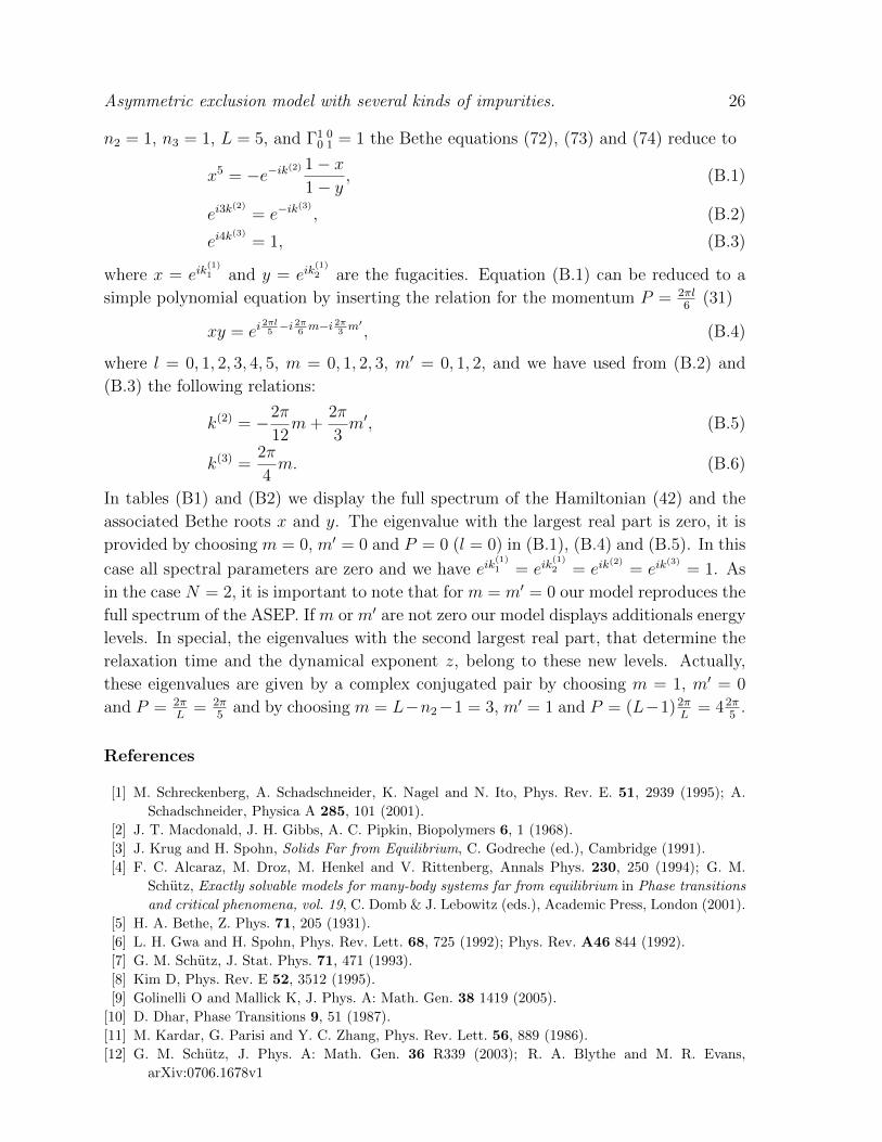
Appendix B. Eigenvalues and Bethe roots for N = 3, n1 = 2, n2 = 1, n3 = 1
and L = 5
In this appendix we list the full spectrum of the Hamiltonian (42) for the asymmetric
exclusion model with one kind of impurities for N = 3, n1 = 2, n2 = 1, n3 = 1, L = 5,
Asymmetric exclusion model with several kinds of impurities. 25
Table A1. The eigenvalues for L = 6, n1 = 2 and n2 = 1
Sector Energies Bethe roots
P = 0, m = 00 1; 1
−1.3819660 0.3090170± 0.9510565i−3.6180340 −0.8090170± 0.5877852i
P = 2π6
, m = 0−0.5074856− 0.2181393i 0.8199801− 0.0796133i; 0.5024902 + 1.1049419i−2.4925144 + 0.2181393i −0.7655328 + 0.7087925i; 0.2122933− 0.9347130i
P = 2 2π6
, m = 0−0.8772838− 0.5974379i 0.5755876 + 0.3275559i; −0.0093985 + 1.5099420i−1.3562417− 0.1208056i 0.7592145− 0.0749922i; −0.7637957 + 1.0652413i−2.7664745 + 0.7182435i −0.9728436− 0.4011708i; 0.1255214− 0.9419611i
P = 3 2π6
, m = 0−1.5 0.6180340; −1.6180340−1.5 −1.6180340; 0.6180340
P = 4 2π6
, m = 0−0.8772838 + 0.5974379i −0.0093985− 1.5099420i; 0.5755876− 0.3275559i−1.3562417 + 0.1208056i 0.7592145 + 0.0749922i; −0.7637957− 1.0652413i−2.7664745− 0.7182435i 0.1255214 + 0.9419611i; −0.9728436 + 0.4011708i
P = 5 2π6
, m = 0−0.5074856 + 0.2181393i 0.8199801 + 0.0796133i; 0.5024902− 1.1049419i−2.4925144− 0.2181393i 0.2122933 + 0.9347130i; −0.7655328− 0.7087925i
P = 0, m = 1−0.6557872 + 0.2961339i 0.7018547− 0.0959405i; 0.1911910− 1.3986613i−2.3442128− 0.2961339i 0.4489168 + 0.8140546i; −0.9419626− 0.5194527i
P = 2π6
, m = 1−0.0572751 + 0.2059994i 0.8373023− 0.0855293i; 1.0839923− 0.4864275i−1.3828654 + 0.0130776i 0.5293573 + 0.8049461i; 0.0602956− 1.0362278i−3.5598595− 0.2190769i −0.6226580 + 0.7713741i; −0.9411875− 0.3629724i
P = 2 2π6
, m = 1−0.4139462− 0.1150956i 0.6884251 + 0.8429321i; 0.8591734− 0.3257069i−2.5860538 + 0.1150956i −0.5524868 + 0.8570897i; −0.0480098− 0.9794781i
P = 3 2π6
, m = 1−0.4977725− 0.5315017i 0.6345797 + 0.2963134i; 0.6041134 + 1.2937589−1.3835508− 0.0616583i 0.7884227− 0.3472311i; −0.4678531 + 1.0623069i−3.1186767 + 0.5931600i −1.0219882− 0.1463166i; −0.1372745− 0.9588315i
P = 4 2π6
, m = 1−1.0832361− 0.2999300i 0.4953389 + 0.1442693i; −1.3406309 + 1.3998737i−1.9167639 + 0.2999300i −1.2180653 + 0.0720208i; 0.7326938− 0.3671649i
P = 5 2π6
, m = 1−1.2103358 + 0.1188691i 0.5489836− 0.0641372i; −1.4512935− 1.0803272i−1.4330978 + 0.6646123i 0.6425791− 0.4326605i; −0.5668353− 1.1597751i−2.3565664− 0.7834814i −0.8735004 + 0.6433986i; 0.3694030 + 0.8445026i
P = 0, m = 2−1.1746854 0.4712748; −2.1219040
−1.9126573− 0.7734344i 0.5609520 + 0.6692321i; −0.7356374 + 0.8776368i−1.9126573 + 0.7734344i 0.5609520− 0.6692321i; −0.7356374− 0.8776368i
P = 2π6
, m = 2−0.8494232 + 0.3327914i 0.5692219− 0.1648546i; −0.4038910− 1.6383922i−2.1505768− 0.3327914i 0.6340571 + 0.6212665i; −1.0851023− 0.3026347i
P = 2 2π6
, m = 2−0.2257571 + 0.3909776i 0.7355889− 0.2131056i; 0.9417640− 0.9044865i−1.3848207 + 0.0309866i 0.6985648 + 0.5996111i; −0.2005790− 1.0675545i−3.3894222− 0.4219643i −0.3934528 + 0.8990944i; −1.0126551− 0.1129670i
P = 3 2π6
, m = 2−0.3819660 0.8090170 + 0.5877853i; 0.8090170− 0.5877853i−2.6180340 −0.3090170 + 0.9510565i; −0.3090170 + 0.9510565i
P = 4 2π6
, m = 2−0.2257571− 0.3909776i 0.7355889 + 0.2131056i; 0.9417640 + 0.9044865i−1.3848207− 0.0309866i −0.2005790 + 1.0675545i; 0.6985648− 0.5996111i−3.3894222 + 0.4219643i −1.0126551 + 0.1129670i; −0.3934528− 0.8990944i
P = 5 2π6
, m = 2−0.8494232− 0.3327914i 0.5692219 + 0.1648546i; −0.4038910 + 1.6383922i−2.1505768 + 0.3327914i 0.6340571− 0.6212665i; −1.0851023 + 0.3026347i
P = 0, m = 3−0.6557872− 0.2961339i 0.7018547 + 0.0959405i; 0.1911910 + 1.3986613i−2.3442128 + 0.2961339i 0.4489168− 0.8140546i; −0.9419626 + 0.5194527i
P = 2π6
, m = 3−1.2103358− 0.1188691i 0.5489836 + 0.0641372i; −1.4512935 + 1.0803272i−1.4330978− 0.6646123i 0.6425791 + 0.4326605i; −0.5668353 + 1.1597751i−2.3565664 + 0.7834814i −0.8735004− 0.6433986i; 0.3694030− 0.8445026i
P = 2 2π6
, m = 3−1.0832361 + 0.2999300i 0.4953389− 0.1442693i; −1.3406309− 1.3998737i−1.9167639− 0.2999300i 0.7326938 + 0.3671649i; −1.2180653− 0.0720208i
P = 3 2π6
, m = 3−0.4977725 + 0.5315017i 0.6345797− 0.2963134i; 0.6041134− 1.2937589−1.3835508 + 0.0616583i 0.7884227 + 0.3472311i; −0.4678531− 1.0623069i−3.1186767− 0.5931600i −1.0219882 + 0.1463166i; −0.1372745 + 0.9588315i
P = 4 2π6
, m = 3−0.4139462 + 0.1150956i 0.8591734 + 0.3257069i; 0.6884251− 0.8429321i−2.5860538− 0.1150956i −0.0480098 + 0.9794781i; −0.5524868− 0.8570897i
P = 5 2π6
, m = 3−0.0572751− 0.2059994i 0.8373023 + 0.0855293i; 1.0839923 + 0.4864275i−1.3828654− 0.0130776i 0.5293573− 0.8049461i; 0.0602956 + 1.0362278i−3.5598595 + 0.2190769i −0.6226580− 0.7713741i; −0.9411875 + 0.3629724i
and Γ1 00 1 = 1. We compared the eigenvalues obtained by direct diagonalization of the
Hamiltonian (42) with those given by the Bethe ansatz solution. For N = 3, n1 = 2,
Asymmetric exclusion model with several kinds of impurities. 26
n2 = 1, n3 = 1, L = 5, and Γ1 00 1 = 1 the Bethe equations (72), (73) and (74) reduce to
x5 = −e−ik(2) 1− x1− y
, (B.1)
ei3k(2)
= e−ik(3)
, (B.2)
ei4k(3)
= 1, (B.3)
where x = eik(1)1 and y = eik
(1)2 are the fugacities. Equation (B.1) can be reduced to a
simple polynomial equation by inserting the relation for the momentum P = 2πl6
(31)
xy = ei2πl5−i 2π
6m−i 2π
3m′ , (B.4)
where l = 0, 1, 2, 3, 4, 5, m = 0, 1, 2, 3, m′ = 0, 1, 2, and we have used from (B.2) and
(B.3) the following relations:
k(2) = −2π
12m+
2π
3m′, (B.5)
k(3) =2π
4m. (B.6)
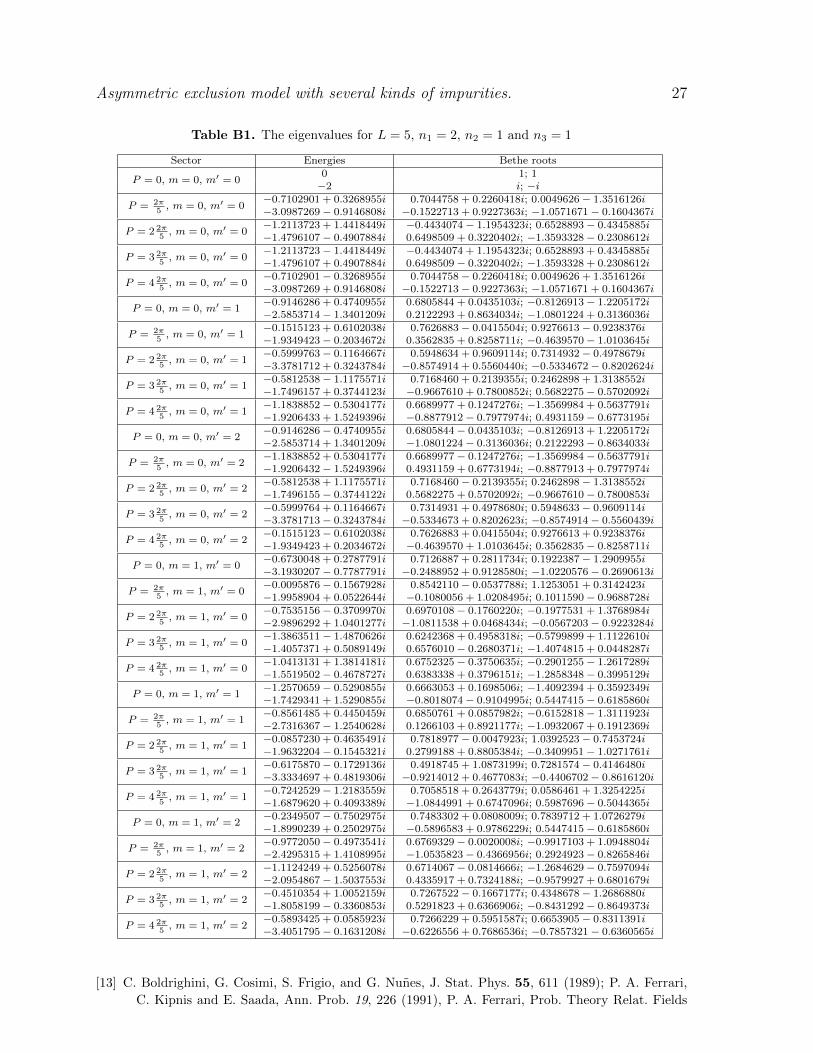
In tables (B1) and (B2) we display the full spectrum of the Hamiltonian (42) and the
associated Bethe roots x and y. The eigenvalue with the largest real part is zero, it is
provided by choosing m = 0, m′ = 0 and P = 0 (l = 0) in (B.1), (B.4) and (B.5). In this
case all spectral parameters are zero and we have eik(1)1 = eik
(1)2 = eik
(2)= eik
(3)= 1. As
in the case N = 2, it is important to note that for m = m′ = 0 our model reproduces the
full spectrum of the ASEP. If m or m′ are not zero our model displays additionals energy
levels. In special, the eigenvalues with the second largest real part, that determine the
relaxation time and the dynamical exponent z, belong to these new levels. Actually,
these eigenvalues are given by a complex conjugated pair by choosing m = 1, m′ = 0
and P = 2πL
= 2π5
and by choosing m = L−n2−1 = 3, m′ = 1 and P = (L−1)2πL
= 42π5
.
References
[1] M. Schreckenberg, A. Schadschneider, K. Nagel and N. Ito, Phys. Rev. E. 51, 2939 (1995); A.
Schadschneider, Physica A 285, 101 (2001).
[2] J. T. Macdonald, J. H. Gibbs, A. C. Pipkin, Biopolymers 6, 1 (1968).
[3] J. Krug and H. Spohn, Solids Far from Equilibrium, C. Godreche (ed.), Cambridge (1991).
[4] F. C. Alcaraz, M. Droz, M. Henkel and V. Rittenberg, Annals Phys. 230, 250 (1994); G. M.
Schutz, Exactly solvable models for many-body systems far from equilibrium in Phase transitions
and critical phenomena, vol. 19, C. Domb & J. Lebowitz (eds.), Academic Press, London (2001).
[5] H. A. Bethe, Z. Phys. 71, 205 (1931).
[6] L. H. Gwa and H. Spohn, Phys. Rev. Lett. 68, 725 (1992); Phys. Rev. A46 844 (1992).
[7] G. M. Schutz, J. Stat. Phys. 71, 471 (1993).
[8] Kim D, Phys. Rev. E 52, 3512 (1995).
[9] Golinelli O and Mallick K, J. Phys. A: Math. Gen. 38 1419 (2005).
[10] D. Dhar, Phase Transitions 9, 51 (1987).
[11] M. Kardar, G. Parisi and Y. C. Zhang, Phys. Rev. Lett. 56, 889 (1986).
[12] G. M. Schutz, J. Phys. A: Math. Gen. 36 R339 (2003); R. A. Blythe and M. R. Evans,
arXiv:0706.1678v1
Asymmetric exclusion model with several kinds of impurities. 27
Table B1. The eigenvalues for L = 5, n1 = 2, n2 = 1 and n3 = 1
Sector Energies Bethe roots
P = 0, m = 0, m′ = 00 1; 1−2 i; −i
P = 2π5
, m = 0, m′ = 0−0.7102901 + 0.3268955i 0.7044758 + 0.2260418i; 0.0049626− 1.3516126i−3.0987269− 0.9146808i −0.1522713 + 0.9227363i; −1.0571671− 0.1604367i
P = 2 2π5
, m = 0, m′ = 0−1.2113723 + 1.4418449i −0.4434074− 1.1954323i; 0.6528893− 0.4345885i−1.4796107− 0.4907884i 0.6498509 + 0.3220402i; −1.3593328− 0.2308612i
P = 3 2π5
, m = 0, m′ = 0−1.2113723− 1.4418449i −0.4434074 + 1.1954323i; 0.6528893 + 0.4345885i−1.4796107 + 0.4907884i 0.6498509− 0.3220402i; −1.3593328 + 0.2308612i
P = 4 2π5
, m = 0, m′ = 0−0.7102901− 0.3268955i 0.7044758− 0.2260418i; 0.0049626 + 1.3516126i−3.0987269 + 0.9146808i −0.1522713− 0.9227363i; −1.0571671 + 0.1604367i
P = 0, m = 0, m′ = 1−0.9146286 + 0.4740955i 0.6805844 + 0.0435103i; −0.8126913− 1.2205172i−2.5853714− 1.3401209i 0.2122293 + 0.8634034i; −1.0801224 + 0.3136036i
P = 2π5
, m = 0, m′ = 1−0.1515123 + 0.6102038i 0.7626883− 0.0415504i; 0.9276613− 0.9238376i−1.9349423− 0.2034672i 0.3562835 + 0.8258711i; −0.4639570− 1.0103645i
P = 2 2π5
, m = 0, m′ = 1−0.5999763− 0.1164667i 0.5948634 + 0.9609114i; 0.7314932− 0.4978679i−3.3781712 + 0.3243784i −0.8574914 + 0.5560440i; −0.5334672− 0.8202624i
P = 3 2π5
, m = 0, m′ = 1−0.5812538− 1.1175571i 0.7168460 + 0.2139355i; 0.2462898 + 1.3138552i−1.7496157 + 0.3744123i −0.9667610 + 0.7800852i; 0.5682275− 0.5702092i
P = 4 2π5
, m = 0, m′ = 1−1.1838852− 0.5304177i 0.6689977 + 0.1247276i; −1.3569984 + 0.5637791i−1.9206433 + 1.5249396i −0.8877912− 0.7977974i; 0.4931159− 0.6773195i
P = 0, m = 0, m′ = 2−0.9146286− 0.4740955i 0.6805844− 0.0435103i; −0.8126913 + 1.2205172i−2.5853714 + 1.3401209i −1.0801224− 0.3136036i; 0.2122293− 0.8634033i
P = 2π5
, m = 0, m′ = 2−1.1838852 + 0.5304177i 0.6689977− 0.1247276i; −1.3569984− 0.5637791i−1.9206432− 1.5249396i 0.4931159 + 0.6773194i; −0.8877913 + 0.7977974i
P = 2 2π5
, m = 0, m′ = 2−0.5812538 + 1.1175571i 0.7168460− 0.2139355i; 0.2462898− 1.3138552i−1.7496155− 0.3744122i 0.5682275 + 0.5702092i; −0.9667610− 0.7800853i
P = 3 2π5
, m = 0, m′ = 2−0.5999764 + 0.1164667i 0.7314931 + 0.4978680i; 0.5948633− 0.9609114i−3.3781713− 0.3243784i −0.5334673 + 0.8202623i; −0.8574914− 0.5560439i
P = 4 2π5
, m = 0, m′ = 2−0.1515123− 0.6102038i 0.7626883 + 0.0415504i; 0.9276613 + 0.9238376i−1.9349423 + 0.2034672i −0.4639570 + 1.0103645i; 0.3562835− 0.8258711i
P = 0, m = 1, m′ = 0−0.6730048 + 0.2787791i 0.7126887 + 0.2811734i; 0.1922387− 1.2909955i−3.1930207− 0.7787791i −0.2488952 + 0.9128580i; −1.0220576− 0.2690613i
P = 2π5
, m = 1, m′ = 0−0.0095876− 0.1567928i 0.8542110− 0.0537788i; 1.1253051 + 0.3142423i−1.9958904 + 0.0522644i −0.1080056 + 1.0208495i; 0.1011590− 0.9688728i
P = 2 2π5
, m = 1, m′ = 0−0.7535156− 0.3709970i 0.6970108− 0.1760220i; −0.1977531 + 1.3768984i−2.9896292 + 1.0401277i −1.0811538 + 0.0468434i; −0.0567203− 0.9223284i
P = 3 2π5
, m = 1, m′ = 0−1.3863511− 1.4870626i 0.6242368 + 0.4958318i; −0.5799899 + 1.1122610i−1.4057371 + 0.5089149i 0.6576010− 0.2680371i; −1.4074815 + 0.0448287i
P = 4 2π5
, m = 1, m′ = 0−1.0413131 + 1.3814181i 0.6752325− 0.3750635i; −0.2901255− 1.2617289i−1.5519502− 0.4678727i 0.6383338 + 0.3796151i; −1.2858348− 0.3995129i
P = 0, m = 1, m′ = 1−1.2570659− 0.5290855i 0.6663053 + 0.1698506i; −1.4092394 + 0.3592349i−1.7429341 + 1.5290855i −0.8018074− 0.9104995i; 0.5447415− 0.6185860i
P = 2π5
, m = 1, m′ = 1−0.8561485 + 0.4450459i 0.6850761 + 0.0857982i; −0.6152818− 1.3111923i−2.7316367− 1.2540628i 0.1266103 + 0.8921177i; −1.0932067 + 0.1912369i
P = 2 2π5
, m = 1, m′ = 1−0.0857230 + 0.4635491i 0.7818977− 0.0047923i; 1.0392523− 0.7453724i−1.9632204− 0.1545321i 0.2799188 + 0.8805384i; −0.3409951− 1.0271761i
P = 3 2π5
, m = 1, m′ = 1−0.6175870− 0.1729136i 0.4918745 + 1.0873199i; 0.7281574− 0.4146480i−3.3334697 + 0.4819306i −0.9214012 + 0.4677083i; −0.4406702− 0.8616120i
P = 4 2π5
, m = 1, m′ = 1−0.7242529− 1.2183559i 0.7058518 + 0.2643779i; 0.0586461 + 1.3254225i−1.6879620 + 0.4093389i −1.0844991 + 0.6747096i; 0.5987696− 0.5044365i
P = 0, m = 1, m′ = 2−0.2349507− 0.7502975i 0.7483302 + 0.0808009i; 0.7839712 + 1.0726279i−1.8990239 + 0.2502975i −0.5896583 + 0.9786229i; 0.5447415− 0.6185860i
P = 2π5
, m = 1, m′ = 2−0.9772050− 0.4973541i 0.6769329− 0.0020008i; −0.9917103 + 1.0948804i−2.4295315 + 1.4108995i −1.0535823− 0.4366956i; 0.2924923− 0.8265846i
P = 2 2π5
, m = 1, m′ = 2−1.1124249 + 0.5256078i 0.6714067− 0.0814666i; −1.2684629− 0.7597094i−2.0954867− 1.5037553i 0.4335917 + 0.7324188i; −0.9579927 + 0.6801679i
P = 3 2π5
, m = 1, m′ = 2−0.4510354 + 1.0052159i 0.7267522− 0.1667177i; 0.4348678− 1.2686880i−1.8058199− 0.3360853i 0.5291823 + 0.6366906i; −0.8431292− 0.8649373i
P = 4 2π5
, m = 1, m′ = 2−0.5893425 + 0.0585923i 0.7266229 + 0.5951587i; 0.6653905− 0.8311391i−3.4051795− 0.1631208i −0.6226556 + 0.7686536i; −0.7857321− 0.6360565i
[13] C. Boldrighini, G. Cosimi, S. Frigio, and G. Nunes, J. Stat. Phys. 55, 611 (1989); P. A. Ferrari,
C. Kipnis and E. Saada, Ann. Prob. 19, 226 (1991), P. A. Ferrari, Prob. Theory Relat. Fields
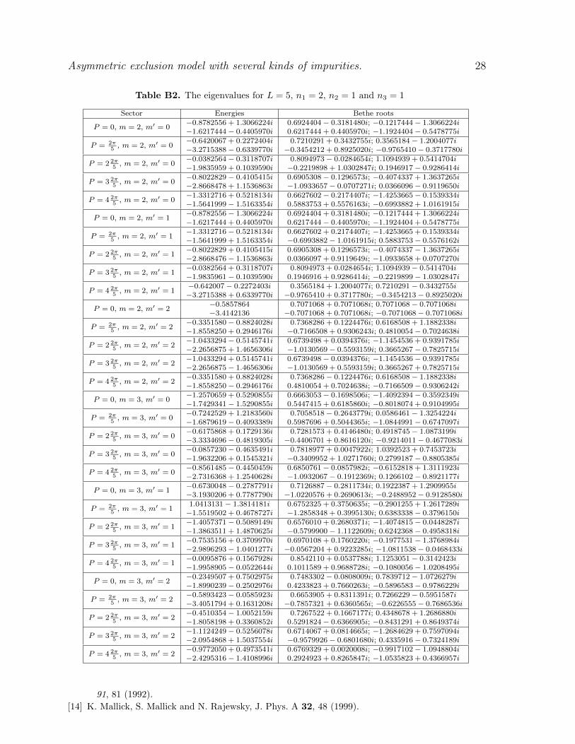
Asymmetric exclusion model with several kinds of impurities. 28
Table B2. The eigenvalues for L = 5, n1 = 2, n2 = 1 and n3 = 1
Sector Energies Bethe roots
P = 0, m = 2, m′ = 0−0.8782556 + 1.3066224i 0.6924404− 0.3181480i; −0.1217444− 1.3066224i−1.6217444− 0.4405970i 0.6217444 + 0.4405970i; −1.1924404− 0.5478775i
P = 2π5
, m = 2, m′ = 0−0.6420067 + 0.2272404i 0.7210291 + 0.3432755i; 0.3565184− 1.2004077i−3.2715388− 0.6339770i −0.3454212 + 0.8925020i; −0.9765410− 0.3717780i
P = 2 2π5
, m = 2, m′ = 0−0.0382564− 0.3118707i 0.8094973− 0.0284654i; 1.1094939 + 0.5414704i−1.9835959 + 0.1039590i −0.2219898 + 1.0302847i; 0.1946917− 0.9286414i
P = 3 2π5
, m = 2, m′ = 0−0.8022829− 0.4105415i 0.6905308− 0.1296573i; −0.4074337 + 1.3637265i−2.8668478 + 1.1536863i −1.0933657− 0.0707271i; 0.0366096− 0.9119650i
P = 4 2π5
, m = 2, m′ = 0−1.3312716 + 0.5218134i 0.6627602− 0.2174407i; −1.4253665− 0.1539334i−1.5641999− 1.5163354i 0.5883753 + 0.5576163i; −0.6993882 + 1.0161915i
P = 0, m = 2, m′ = 1−0.8782556− 1.3066224i 0.6924404 + 0.3181480i; −0.1217444 + 1.3066224i−1.6217444 + 0.4405970i 0.6217444− 0.4405970i; −1.1924404 + 0.5478775i
P = 2π5
, m = 2, m′ = 1−1.3312716− 0.5218134i 0.6627602 + 0.2174407i; −1.4253665 + 0.1539334i−1.5641999 + 1.5163354i −0.6993882− 1.0161915i; 0.5883753− 0.5576162i
P = 2 2π5
, m = 2, m′ = 1−0.8022829 + 0.4105415i 0.6905308 + 0.1296573i; −0.4074337− 1.3637265i−2.8668476− 1.1536863i 0.0366097 + 0.9119649i; −1.0933658 + 0.0707270i
P = 3 2π5
, m = 2, m′ = 1−0.0382564 + 0.3118707i 0.8094973 + 0.0284654i; 1.1094939− 0.5414704i−1.9835961− 0.1039590i 0.1946916 + 0.9286414i; −0.2219899− 1.0302847i
P = 4 2π5
, m = 2, m′ = 1−0.642007− 0.2272403i 0.3565184 + 1.2004077i; 0.7210291− 0.3432755i−3.2715388 + 0.6339770i −0.9765410 + 0.3717780i; −0.3454213− 0.8925020i
P = 0, m = 2, m′ = 2−0.5857864 0.7071068 + 0.7071068i; 0.7071068− 0.7071068i−3.4142136 −0.7071068 + 0.7071068i; −0.7071068− 0.7071068i
P = 2π5
, m = 2, m′ = 2−0.3351580− 0.8824028i 0.7368286 + 0.1224476i; 0.6168508 + 1.1882338i−1.8558250 + 0.2946176i −0.7166508 + 0.9306243i; 0.4810054− 0.7024638i
P = 2 2π5
, m = 2, m′ = 2−1.0433294− 0.5145741i 0.6739498 + 0.0394376i; −1.1454536 + 0.9391785i−2.2656875 + 1.4656306i −1.0130569− 0.5593159i; 0.3665267− 0.7825715i
P = 3 2π5
, m = 2, m′ = 2−1.0433294 + 0.5145741i 0.6739498− 0.0394376i; −1.1454536− 0.9391785i−2.2656875− 1.4656306i −1.0130569 + 0.5593159i; 0.3665267 + 0.7825715i
P = 4 2π5
, m = 2, m′ = 2−0.3351580 + 0.8824028i 0.7368286− 0.1224476i; 0.6168508− 1.1882338i−1.8558250− 0.2946176i 0.4810054 + 0.7024638i; −0.7166509− 0.9306242i
P = 0, m = 3, m′ = 0−1.2570659 + 0.5290855i 0.6663053− 0.1698506i; −1.4092394− 0.3592349i−1.7429341− 1.5290855i 0.5447415 + 0.6185860i; −0.8018074 + 0.9104995i
P = 2π5
, m = 3, m′ = 0−0.7242529 + 1.2183560i 0.7058518− 0.2643779i; 0.0586461− 1.3254224i−1.6879619− 0.4093389i 0.5987696 + 0.5044365i; −1.0844991− 0.6747097i
P = 2 2π5
, m = 3, m′ = 0−0.6175868 + 0.1729136i 0.7281573 + 0.4146480i; 0.4918745− 1.0873199i−3.3334696− 0.4819305i −0.4406701 + 0.8616120i; −0.9214011− 0.4677083i
P = 3 2π5
, m = 3, m′ = 0−0.0857230− 0.4635491i 0.7818977 + 0.0047922i; 1.0392523 + 0.7453723i−1.9632206 + 0.1545321i −0.3409952 + 1.0271760i; 0.2799187− 0.8805385i
P = 4 2π5
, m = 3, m′ = 0−0.8561485− 0.4450459i 0.6850761− 0.0857982i; −0.6152818 + 1.3111923i−2.7316368 + 1.2540628i −1.0932067− 0.1912369i; 0.1266102− 0.8921177i
P = 0, m = 3, m′ = 1−0.6730048− 0.2787791i 0.7126887− 0.2811734i; 0.1922387 + 1.2909955i−3.1930206 + 0.7787790i −1.0220576 + 0.2690613i; −0.2488952− 0.9128580i
P = 2π5
, m = 3, m′ = 11.0413131− 1.3814181i 0.6752325 + 0.3750635i; −0.2901255 + 1.2617289i−1.5519502 + 0.4678727i −1.2858348 + 0.3995130i; 0.6383338− 0.3796150i
P = 2 2π5
, m = 3, m′ = 1−1.4057371− 0.5089149i 0.6576010 + 0.2680371i; −1.4074815− 0.0448287i−1.3863511 + 1.4870625i −0.5799900− 1.1122609i; 0.6242368− 0.4958318i
P = 3 2π5
, m = 3, m′ = 1−0.7535156 + 0.3709970i 0.6970108 + 0.1760220i; −0.1977531− 1.3768984i−2.9896293− 1.0401277i −0.0567204 + 0.9223285i; −1.0811538− 0.0468433i
P = 4 2π5
, m = 3, m′ = 1−0.0095876 + 0.1567928i 0.8542110 + 0.0537788i; 1.1253051− 0.3142423i−1.9958905− 0.0522644i 0.1011589 + 0.9688728i; −0.1080056− 1.0208495i
P = 0, m = 3, m′ = 2−0.2349507 + 0.7502975i 0.7483302− 0.0808009i; 0.7839712− 1.0726279i−1.8990239− 0.2502976i 0.4233823 + 0.7660263i; −0.5896583− 0.9786229i
P = 2π5
, m = 3, m′ = 2−0.5893423− 0.0585923i 0.6653905 + 0.8311391i; 0.7266229− 0.5951587i−3.4051794 + 0.1631208i −0.7857321 + 0.6360565i; −0.6226555− 0.7686536i
P = 2 2π5
, m = 3, m′ = 2−0.4510354− 1.0052159i 0.7267522 + 0.1667177i; 0.4348678 + 1.2686880i−1.8058198 + 0.3360852i 0.5291824− 0.6366905i; −0.8431291 + 0.8649374i
P = 3 2π5
, m = 3, m′ = 2−1.1124249− 0.5256078i 0.6714067 + 0.0814665i; −1.2684629 + 0.7597094i−2.0954868 + 1.5037554i −0.9579926− 0.6801680i; 0.4335916− 0.7324189i
P = 4 2π5
, m = 3, m′ = 2−0.9772050 + 0.4973541i 0.6769329 + 0.0020008i; −0.9917102− 1.0948804i−2.4295316− 1.4108996i 0.2924923 + 0.8265847i; −1.0535823 + 0.4366957i
91, 81 (1992).
[14] K. Mallick, S. Mallick and N. Rajewsky, J. Phys. A 32, 48 (1999).
Asymmetric exclusion model with several kinds of impurities. 29
[15] B. Sutherland, Phys. Rev. B20, 3795 (1975).
[16] P. Schlottmann, Phys. Rev. B36, 5177 (1987).
[17] J. H. H. Perk and C. L. Schultz, Phys. Lett. A 84, 407 (1981).
[18] F. H. L. Essler, V. E. Korepin and K. Schoutens, Phys. Rev. Lett. 68 2960 (1992); Phys. Rev.
Lett. 70 73 (1993).
[19] E. H. Lieb and F. Y. Wu, Phys. Rev. Lett. 20 1445 (1968).
[20] F. C. Alcaraz and R. Z. Bariev, J. Phys. A: Math. Gen. 32 L483 (1999).
[21] V. Popkov, M. E. Fouladvand and G. M. Schutz, J. Phys. A: Math. Gen 35, 7187 (2002);
[22] M. J. Lazo, Braz. J. Phys. 38 237 (2008).
[23] Lazo M J and Ferreira A A, Phys. Rev. E 81 050104 (2010).
[24] F. C. Alcaraz and M. J. Lazo, J. Phys. A: Math. Gen. 39 11335 (2006); J. Phys. A: Math. Gen.
37 L1 (2004); J. Phys. A: Math. Gen. 37 4149 (2004); Braz. J. Phys. 33 533 (2003).
[25] Zamolodchikov A B Commun. Math. Phys. 69 165 (1979); Zamolodchikov A B and Zamolodchikov
Al B Ann. Phys. 120 253 (1979).
[26] F. C. Alcaraz, D. Arnaudon, V. Rittenberg and M. Scheunert, Int. J. of Mod. Phys. A9 3473
(1994).
[27] O. Golinelli and K. Mallick, J. Phys. A: Math. Gen. 39 10647 (2006).
[28] B. Derrida, M. R. Evans, V. Hakim and V. Pasquier, J. Phys. A: Math. Gen. 26 1493 (1993).


![(2016) Two kinds of 'and' [26/2/2016]](https://img.dokumen.tips/doc/110x75/6353f0329ef77da538047641/2016-two-kinds-of-and-2622016.jpg)


