Deterministic chaos in atmospheric radon dynamics

(half-life of 3.8 days),and 220Rn, called thoron (half-life of 55 s),

17,962 CUCULEANU AND LUPU: CHAOS IN ATMOSPHERIC RADON DYNAMICS

methods to determine the geometrical and dynamical characteristics of their attractors in order to see whether these

isotopes could trace the chaotic behavior of the atmosphere as well. In addition to a noninteger (correlation) dimension for the attractor, positive Lyapunov exponents and positive, finite Kolmogorov entropy are basic quantities highlighting the deterministic chaos in a time series of a physical observ- able. The purpose of this paper is to study the geometrical and dynamical characteristics of the atmospheric radon attractors by using 5-hour average concentration time series measured at the Atmospheric Physics Laboratory of the Na- tional Institute of Meteorology and Hydrology located near Bucharest. These characteristics may be related to the turbulence features within the lower atmosphere subsystems. Such findings may contribute to a better understanding of the atmospheric dynamics within the layer near the ground and, consequently, of aerosol and trace gas transport. In this re-

tions describing the accumulation and decay of nuclei during the air filtering, the decay when filtering ceases, and an appropriate sequence of measurements for each filter. By taking into account the radioactive equilibrium assumption, the 222Rn activity concentration can be deduced. A number of activity concentration values (5832) of 22øRn and 222Rn daughters have been obtained from four daily measurements during a 4-year period (1993-1996) at the Observatory for Atmospheric Physics located near Bucharest. Four aerosol samplings of 5 hours were carried out daily at 0200-0700, 0800-1300, 1400-1900, and 2000-0100 UT. The 5-hour as- piration is related to the fact that the measuring program was intended for the determination of artificial radioactiv-

ity as well. From the point of view of our analysis, the four measurements provide an adequate sampling of the boundary layer, covering the whole range of atmospheric stability states in their diurnal variation [Beck and Gogolak, 1979].

spect, the relevant results refer to the number of independent The statistical errors range between 0.5 and 2%. Owing to variables necessary to describe the diffusion of the atmospheric constituents as well as to estimate the atmospheric predictability (error doubling) time.

In section 2, considerations on the time series of 222Rn and 22øRn daughter concentrations are presented. A discussion regarding the characteristics used to reveal the deterministic chaos is given in section 3. The results obtained are presented in section 4, and their interpretation and conclusions are discussed in section 5.

this very low value, the stochastic nature of the radioactive decay does not affect the geometrical and dynamical characteristics of the analyzed systems, the prevailing factor being the atmospheric variability, and the classical theory of dynamical systems can be safely applied. The errors due to the reference standard, to the air flow rate determination, and to

filter efficiency have a maximum estimated value of 20% for some measured concentrations. More details on the mea-

surement technique are given by Cuculeanu et al. [ 1992].

2. Time Series of Radon and Thoron

Concentrations

Under most meteorological conditions, the short-lived 222Rn daughters are in secular radioactive equilibrium with atmospheric 222Rn [Schmidt et al., 1996; PorstendO'rfer, 1993]. Therefore the atmospheric 222Rn (gas) activity can be determined via the activity of its short-lived aerosol-attached daughters. In the case of 22øRn daughters, according to Ja- cobi and Andrd's [ 1963] model, irrespective of turbulence conditions, there is no equilibrium with 22øR• except at a point whose altitude varies from 1 m (strong inversion) to •100 m (strong mixing). But an approximate radioactive equilibrium can be considered for 2•2Bi relative to 2•2pb within the surface layer [United Nations Scientific Commit- tee on the Effects of Atomic Radiation, 1982]. Even if a cer- tain disequilibrium exists between 22øRn and its daughters, the bulk concentration of the main daughter (2•2pb) is found in the immediate vicinity of the precursor (22øRn); therefore one may assume that the daughter dynamics reflects the precursor dynamics. The measuring method of the daughter activity concentrations is based on aerosol collection on filters by means of an air-filtering device having the aspi- ration head at 2 m above the ground. Th• filter activity has been determined by using low background beta global measuring equipment manufactured by Nuclear Enterprises, with G-M counter tubes with 2 counts min -• background in anticoincidence. Strontium 90/yttrium 90 was used as a reference standard. In order to obtain the daughter activity concentrations, a model for processing the filter activ- ities has been developed by taking into account the equa-

3. Characteristics Indicating Chaotic Behavior

In order to reveal the presence of the chaos in the dynamics of a time series, the correlation dimension, the Lyapunov exponents, and the entropy have to be determined. A quali- tative indication upon the dynamics underlying a time series is provided by the power spectrum which has to be broadband in the case of a chaotic system. There may be peaks sitting on the top of the broadband noise, which highlight different periods embedded in the chaotic signal. On the other hand, the onset of the broadband spectrum cannot al- ways serve as confirmation of chaos because noisy periodic or quasiperiodic signals can be characterized by a broadband power spectrum, too.

3.1. Phase Space Reconstruction

Let {:ri = 2(ti)}i=l,N represent the time series of atmospheric radon concentrations, where ti = ti-1 + p + At, tl is starting time of the measurements, p is the time interval between the end of filter sampling and the beginning of the next measurement, At is the sampling time, and N is the total number of measurements. It has been shown by Takens [ 1981 ] that from a single time series one can properly recon- struct an m-dimensional phase space by taking the original time series .•(ti) and its successive time shifts (delays) as coordinates of a vector time series given by

Xi: {x(ti),x(ti + •-),...,x[ti + (m- 1)7-]}, (1)

where m is the dimension of the vector Xi, often referred to as the embedding dimension, and v- is the time delay. If v-

CUCULEANU AND LUPU' CHAOS IN ATMOSPHERIC RADON DYNAMICS 17,963

6000 , , 100000

5000 80000

4000

60000 , I, 3000 • ' '

:• 40000 2000 •'

20000 1000

0 0 0 200 400 600 800 1000 0 200 400 600 800 1000

Time (units of 6 h) Time (units of 6 h)

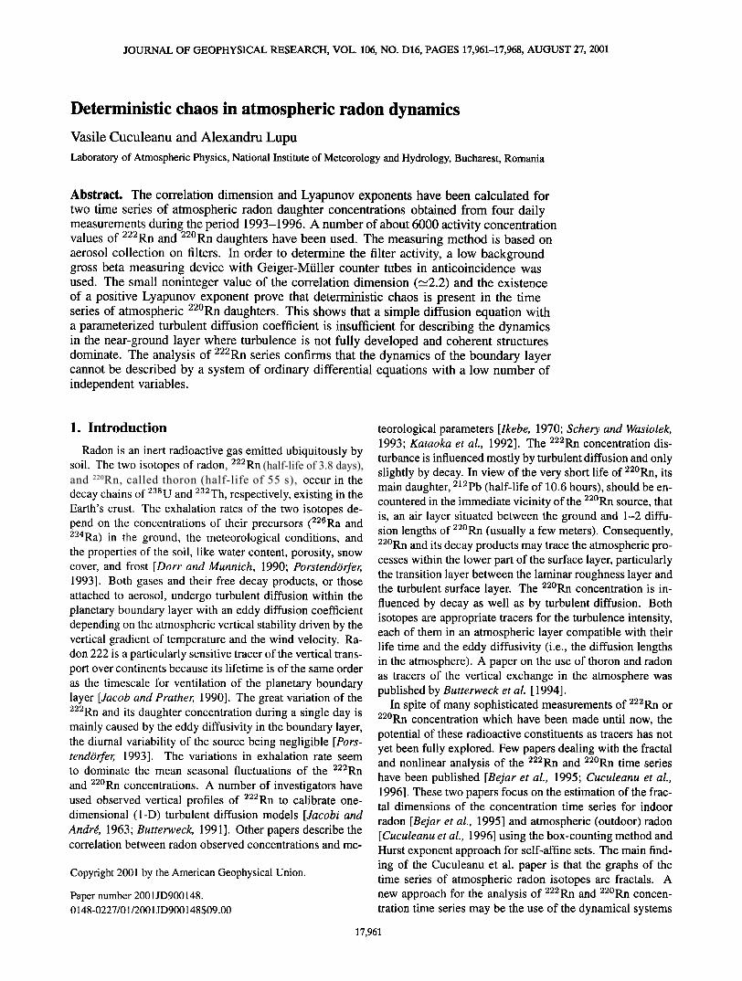
Figure 1. Time series of (left) 22øRn and (right) 222Rn.

is properly chosen, the variables x(t•), x(ti q- r), ..., x[ti q- (m - 1)r] will be independent, this being all one needs to define a phase space. The typical choice of r is based on the decorrelation time of the time series under study. We define r as the lag time at which the autocorrelation function first falls below a threshold value which is commonly taken as e -• in meteorology [Zeng et al., 1992]. A quite reasonable objection to this procedure is that it is based on linear statistics. That is why the mutual information, which takes into account nonlinear dynamical correlations, has been used as an additional procedure to determine r. Thus a good candi- date for a reasonable time delay is the value of r at which the time-delayed mutual information exhibits the first minimum [Fraser and Swinney, 1986].

3.2. Correlation Dimension

For a fixed embedding dimension m, the time series of vectors X, in the embedding space is used to calculate the correlation sum defined as the fraction of all possible pairs of points (Xj, Xi•) which are closer than a given distance e in a particular norm [Kantz and Schreiber, 1997]:

N

Crn(e) -- ]Vpair s • Z {•)(• -IIx,- x11), (2) 3=m k <j-w

where l•pairs -- (X- //g q- 1)(X-//g- w q- 1)/2, {•)is the Heaviside step function, and w is the Theiler window [Theiler, 1986].

For values of the scale e much smaller than the linear size

of the attractor but larger than scales where measurement error or noise are important, it can be shown that the depen- dence of Urn(e) upon e is given by [Grassberger and Pro- caccia, 1983]

(3) Temporally correlated points have been excluded by discard- ing the pairs of points closer together in time than Theiler's window w. To estimate a safe value for Theiler's window,

a space-time separation plot was used [Provenzale et al., 1992]. Proper handling of temporal correlations certifies that the scaling, if present, is genuine. For each embedding dimension m, the exponent d is estimated from the slope of the linear region of the plot of In Cm (e) versus Ine. If d ap- proaches a value D, independent of m, this value D is called the correlation dimension of the attractor. The dimension M

1

0.8

0.6

0.4 0.2

0

-0.2 0 5o

1

0.8

• 0.6

o 0.4 o

• 0.2

0

-0.2 200 0

i i i i

100 150 50 100 150 200

Time (units of 6 h) Time (units of 6 h)

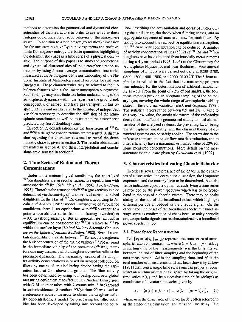
Figure 2. Autocorrelation function for (left) 22øRn and (right) 222Rn time series.


le+06. le+08 .....

100000

E

• 10000

o

lOOO

lOO i I I I I I

0 0.2 0.4 0.6 0.8 I 1.2 1.4 1.6 1.8

Frequency (1/d)

le+07

E

• le+06

o

100000

10000 • • • • • • • • ' 2 0 0.2 0.4 0.6 0.8 1 1.2 1.4 1.6 1.8

Frequency (1/d)

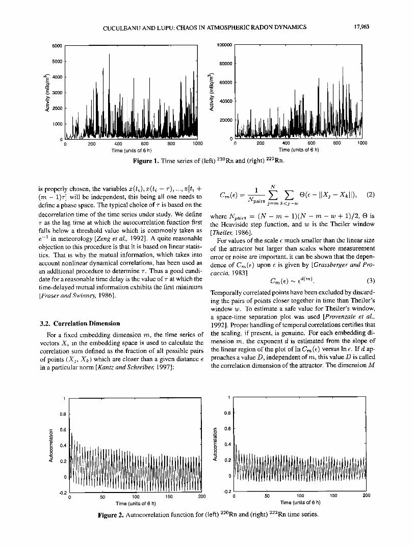
Figure 3. Power spectrum for (left) 22øRn and (right) 222Rn time series.

of m above which d no longer changes is the (minimum) embedding dimension.

3.3. Lyapunov Exponents

A quantitative measure of the sensitivity to the initial conditions is provided by the Lyapunov exponents. There exists as many Lyapunov exponents as phase space dimensions. If the dynamical system is chaotic, there will be at least one positive Lyapunov exponent. In addition, for any continuous chaotic process, there must be at least one exponent identical

to zero. In this paper only the largest positive exponent has been calculated by using the algorithm proposed by Kantz and Schreiber [ 1997], which allows the calculation of this exponent for separations of nearby trajectories in the recon- structed space lying in the linear region with saturated slope. The algorithm consists of choosing a point X,• o of the time series in embedding space and selecting all neighbors with distance smaller than •. The average over the distances of all neighbors to the reference part of the trajectory as a function of the relative time has been computed. The average over no of the logarithm of the average distance at time An -- n-no is the expansion rate S(•, m, An) over the time span An (plus the logarithm of the initial distance). If for some range

of An the function $ exhibits a robust linear increase, its slope is an estimate of the maximal Lyapunov exponent •. The sum of the positive exponents gives an estimate of the Kolmogorov entropy.

4. Results

4.1. Autocorrelation Function

Figure 1 shows the time series of 22øRn daughters and 222Rn, and Figure 2 shows the corresponding autocorrelation functions. Both series exhibit similar patterns. As was stated in section 3.1, two procedures have been used to determine the time delay. The procedure based on the autocorrelation function gives r = 1.1 (units of 6 hours) for the 22øRn time series and r = 0.95 (units of 6 hours) for the 222Rn time series. None of the autocorrelation functions falls to zero

within a very short time. This is an indication that neither of the time series displays the signs of a completely random behavior, because for the Gaussian white noise, the zero of the autocorrelation function is immediately attained (for r = 1 the autocorrelation function is already equal to -0.02). On the other hand, the mutual information for both time series exhibits a minimum at r = 2. Since both procedures yield

i 1

0.1 0.1

0.01 = 0.01

0.001

0.001

0.0001 le-05

I e-05 1 e-06

I e-06 I e-07

le-07 le-08 10 100 1000 10 100 1000 10000 100000

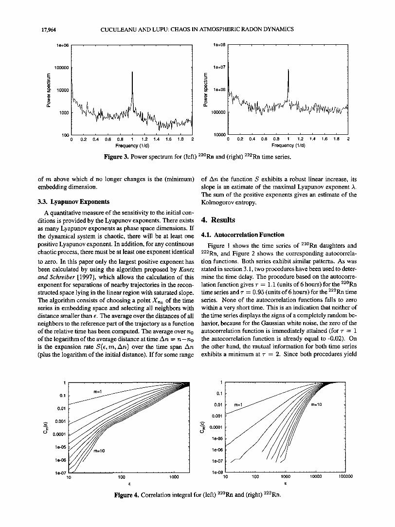
Figure 4. Correlation integral for (left) 22øRn and (right) 222Rn.

CUCULEANU AND LUPU: CHAOS IN ATMOSPHERIC RADON DYNAMICS 17,965

10

•x m=l 0

10 1 O0 1000

m=10

i

0 1 O0 1000 10000 100000

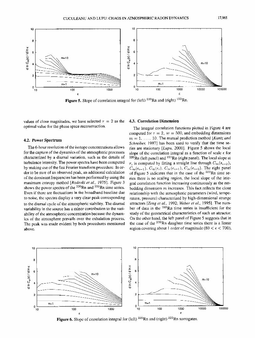
Figure 5. Slope of correlation integral for (left) 22øRn and (right) 222Rn.

values of close magnitudes, we have selected 7- - 2 as the optimal value for the phase space reconstruction.

4.2. Power Spectrum

The 6-hour resolution of the isotope concentrations allows for the capture of the dynamics of the atmospheric processes characterized by a diurnal variation, such as the details of turbulence intensity. The power spectra have been computed by making use of the fast Fourier transform procedure. In order to be sure of an observed peak, an additional calculation of the dominant frequencies has been performed by using the maximum entropy inethod [Rodoski et al., 1975]. Figure 3 shows the power spectra of the 22øRn and 222Rn time series. Even if there arc fluctuations in the broadband baseline due

to noise, the spectra display a very clear peak corresponding to the diurnal cycle of the atmospheric stability. The diurnal variability in the source has a minor contribution to the variability of the atmospheric concentration because the dynamics of the atmosphere prevails over the exhalation process. The peak was made evident by both procedures mentioned above.

4.3. Correlation Dimension

The integral correlation functions plotted in Figure 4 are computed for 7- - 2, w - 500, and embedding dimensions m = 1 ..... 10. The mutual prediction method [Kantz and Schreiber, 1997] has been used to verify that the time series are stationary [Lupu, 2000]. Figure 5 shows the local slope of the correlation integral as a function of scale • for 22øRn (left panel) and 222Rn (right panel). The local slope at ri is computed by fitting a straight line through Cm(•i-2), Cm(e•-l), Cm(6•), Cm(•i+l), Cm(6i42). The right panel of Figure 5 indicates that in the case of the 222Rn time series there is no scaling region, the local slope of the integral correlation function increasing continuously as the embedding dimension m increases. This fact reflects the close relationship with the atmospheric parameters (wind, temperature, pressure) characterized by high-dimensional strange attractors [Zeng et al., 1992; Weber et al., 1995]. The number of data in the 222Rn time series is insufficient for the

study of the geometrical characteristics of such an attractor. On the other hand, the left panel of Figure 5 suggests that in the case of the •øRn daughter time series there is a linear region covering about 1 order of magnitude (80 < • < 700),

"xx%•%.,. m=10

_-

i

o 1 oo 1 ooo 1 o 1 oo 1 ooo 1 oooo 1 ooooo

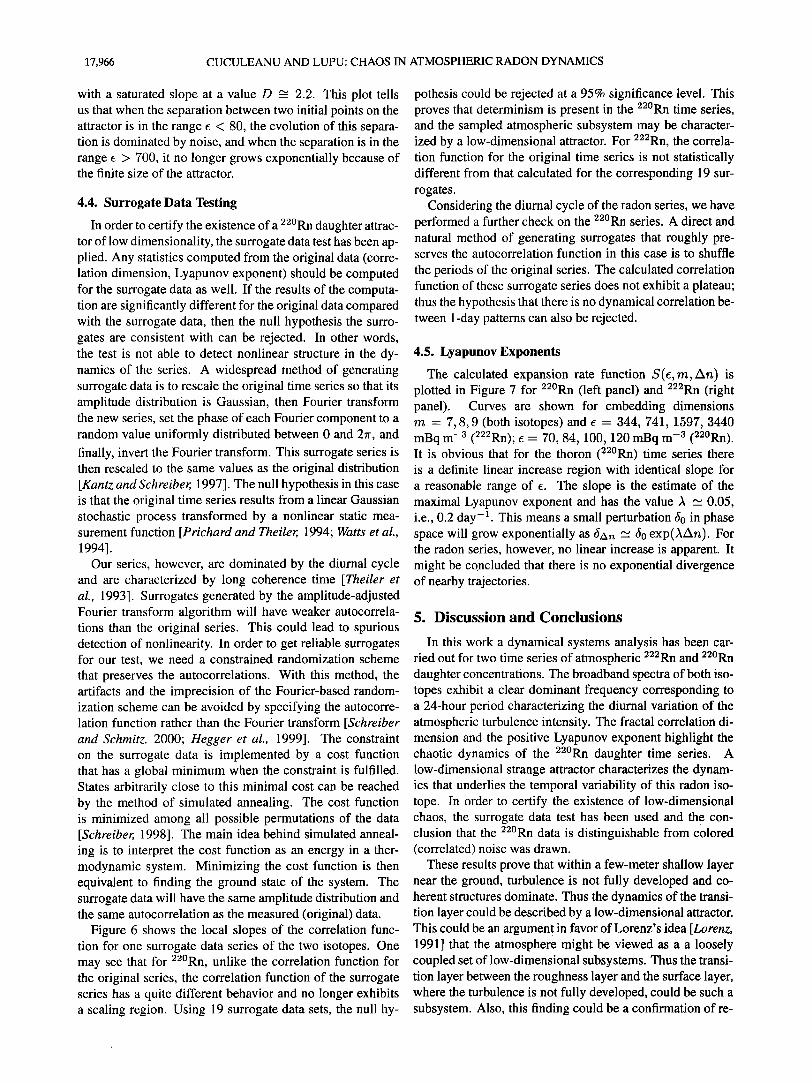
Figure 6. Slope of correlation integral for (left) 22øRn and (right) 222Rn surrogates.


with a saturated slope at a value D --- 2.2. This plot tells us that when the separation between two initial points on the attractor is in the range • < 80, the evolution of this separation is dominated by noise, and when the separation is in the range • > 700, it no longer grows exponentially because of the finite size of the attractor.

4.4. Surrogate Data Testing

In order to certify the existence of a 22øRn daughter attractor of low dimensionality, the surrogate data test has been applied. Any statistics computed from the original data (correlation dimension, Lyapunov exponent) should be computed for the surrogate data as well. If the results of the computa- tion are significantly different for the original data compared with the surrogate data, then the null hypothesis the surrogates are consistent with can be rejected. In other words, the test is not able to detect nonlinear structure in the dynamics of the series. A widespread method of generating surrogate data is to rescale the original time series so that its amplitude distribution is Gaussian, then Fourier transform the new series, set the phase of each Fourier component to a random value uniformly distributed between 0 and 2•r, and

finally, invert the Fourier transform. This surrogate series is then rescaled to the same values as the original distribution [Kantz and Schreiber, 1997]. The null hypothesis in this case is that the original time series results from a linear Gaussian stochastic process transformed by a nonlinear static measurement function [Prichard and Theiler, 1994; Watts et al., 1994].

Our series, however, are dominated by the diurnal cycle and are characterized by long coherence time [Theiler et al., 1993]. Surrogates generated by the amplitude-adjusted Fourier transform algorithm will have weaker autocorrelations than the original series. This could lead to spurious detection of nonlinearity. In order to get reliable surrogates for our test, we need a constrained randomization scheme

that preserves the autocorrelations. With this method, the artifacts and the imprecision of the Fourier-based randomization scheme can be avoided by specifying the autocorrelation function rather than the Fourier transform [Schreiber and Schmitz, 2000; Hegger et al., 1999]. The constraint on the surrogate data is implemented by a cost function that has a global minimum when the constraint is fulfilled. States arbitrarily close to this minimal cost can be reached by the method of simulated annealing. The cost function is minimized among all possible permutations of the data [Schreiber, 1998]. The main idea behind simulated annealing is to interpret the cost function as an energy in a ther- modynamic system. Minimizing the cost function is then equivalent to finding the ground state of the system. The surrogate data will have the same amplitude distribution and the same autocorrelation as the measured (original) data.

Figure 6 shows the local slopes of the correlation function for one surrogate data series of the two isotopes. One may see that for 22øRn, unlike the correlation function for the original series, the correlation function of the surrogate series has a quite different behavior and no longer exhibits a scaling region. Using 19 surrogate data sets, the null hy-

pothesis could be rejected at a 95% significance level. This proves that determinism is present in the 22øRn time series, and the sampled atmospheric subsystem may be characterized by a low-dimensional attractor. For 222Rn, the correlation function for the original time series is not statistically different from that calculated for the corresponding 19 surrogates.

Considering the diurnal cycle of the radon series, we have performed a further check on the 22øRn series. A direct and natural method of generating surrogates that roughly preserves the autocorrelation function in this case is to shuffle

the periods of the original series. The calculated correlation function of these surrogate series does not exhibit a plateau; thus the hypothesis that there is no dynamical correlation between 1-day patterns can also be rejected.

4.5. Lyapunov Exponents

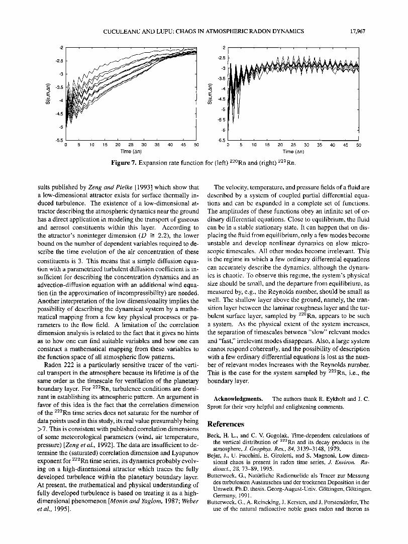
The calculated expansion rate function S(e,m, An) is plotted in Figure 7 for 22øRn (left panel) and 222Rn (right panel). Curves are shown for embedding dimensions m = 7, 8, 9 (both isotopes) and e = 344, 741, 1597, 3440 mBq m -3 (222Rn); e = 70, $4, 100,120 mBq m -3 (22øRn). It is obvious that for the thoron (22øRn) time series there is a definite linear increase region with identical slope for a reasonable range of e. The slope is the estimate of the maximal Lyapunov exponent and has the value A _• 0.05, i.e., 0.2 day -1. This means a small perturbation t•0 in phase space will grow exponentially as t•/xn -• t•0 exp(•An). For the radon series, however, no linear increase is apparent. It might be concluded that there is no exponential divergence of nearby trajectories.

5. Discussion and Conclusions

In this work a dynamical systems analysis has been carried out for two time series of atmospheric 222Rn and 22øRn daughter concentrations. The broadband spectra of both isotopes exhibit a clear dominant frequency corresponding to a 24-hour period characterizing the diurnal variation of the atmospheric turbulence intensity. The fractal correlation dimension and the positive Lyapunov exponent highlight the chaotic dynamics of the 22øRn daughter time series. A low-dimensional strange attractor characterizes the dynamics that underlies the temporal variability of this radon isotope. In order to certify the existence of low-dimensional chaos, the surrogate data test has been used and the con- clusion that the 22øRn data is distinguishable from colored (correlated) noise was drawn.

These results prove that within a few-meter shallow layer near the ground, turbulence is not fully developed and co- herent structures dominate. Thus the dynamics of the transi- tion layer could be described by a low-dimensional attractor. This could be an argument in favor of Lorenz's idea [Lorenz, 1991] that the atmosphere might be viewed as a a loosely coupled set of low-dimensional subsystems. Thus the transi- tion layer between the roughness layer and the surface layer, where the turbulence is not fully developed, could be such a subsystem. Also, this finding could be a confirmation of re-

CUCULEANU AND LUPU: CHAOS IN ATMOSPHERIC RADON DYNAMICS 17,967

-2.5

c -3.5

• -4

-4.5

-5.5

-2 [ , , -2.5

-3

-3.5

•' -4

•. -4.5 -5

-5.5

' • ' ' ' ' -6.5 ' ' • ' ' ' ' 20 25 30 35 40 45 50 0 5 10 15 20 25 30 35 40 45

Time (An) Time (An)

Figure 7. Expansion rate function for (left) 22øRn and (right) 222Rn.

sults published by Zeng and Pielke [1993] which show that a low-dimensional attractor exists for surface thermally in- duced turbulence. The existence of a low-dimensional at-

tractor describing the atmospheric dynamics near the ground has a direct application in modeling the transport of gaseous and aerosol constituents within this layer. According to the attractor's noninteger dimension (D - 2.2), the lower bound on the number of dependent variables required to describe the time evolution of the air concentration of these

constituents is 3. This means that a simple diffusion equation with a parametrized turbulent diffusion coefficient is insufficient for describing the concentration dynamics and an advection-diffusion equation with an additional wind equation (in the approximation of incompressibility) are needed. Another interpretation of the low dimensionality implies the possibility of describing the dynamical system by a mathematical mapping from a few key physical processes or parameters to the flow field. A limitation of the correlation

dimension analysis is related to the fact that it gives no hints as to how one can find suitable variables and how one can

construct a mathematical mapping from these variables to the function space of all atmospheric flow patterns.

Radon 222 is a particularly sensitive tracer of the vertical transport in the atmosphere because its lifetime is of the same order as the timescale for ventilation of the planetary boundary layer. For 2'2'2'Rn, turbulence conditions are dominant in establishing its atmospheric pattern. An argument in favor of this idea is the fact that the correlation dimension

of the 2'2'2Rn time series does not saturate for the number of

data points used in this study, its real value presumably being > 7. This is consistent with published correlation dimensions of some meteorological parameters (wind, air temperature, pressure) [Zeng et al., 1992]. The data are insufficient to determine the (saturated) correlation dimension and Lyapunov exponent for 22'2Rn time series, its dynamics probably evolv- ing on a high-dimensional attractor which traces the fully developed turbulence within the planetary boundary layer. At present, the mathematical and physical understanding of fully developed turbulence is based on treating it as a high- dimensional phenomenon [Monin and Yaglom, 1987; Weber et al., 1995].

The velocity, temperature, and pressure fields of a fluid are described by a system of coupled partial differential equations and can be expanded in a complete set of functions. The amplitudes of these functions obey an infinite set of ordinary differential equations. Close to equilibrium, the fluid can be in a stable stationary state. It can happen that on dis- placing the fluid from equilibrium, only a few modes become unstable and develop nonlinear dynamics on slow micro- scopic timescales. All other modes become irrelevant. This is the regime in which a few ordinary differential equations can accurately describe the dynamics, although the dynamics is chaotic. To observe this regime, the system's physical size should be small, and the departure from equilibrium, as measured by, e.g., the Reynolds number, should be small as well. The shallow layer above the ground, namely, the tran- sition layer between the laminar roughness layer and the turbulent surface layer, sampled by 22øRn, appears to be such a system. As the physical extent of the system increases, the separation of timescales between "slow" relevant modes and "fast," irrelevant modes disappears. Also, a large system cannot respond coherently, and the possibility of description with a few ordinary differential equations is lost as the number of relevant modes increases with the Reynolds number. This is the case for the system sampled by 222Rn, i.e., the boundary layer.

Acknowledgments. The authors thank R. Eykholt and J. C. Sprott for their very helpful and enlightening comments.

References

Beck, H. L., and C. V. Gogolak, Time-dependent calculations of the vertical distribution of 222Rn and its decay products in the atmosphere, J. Geophys. Res., 84, 3139-3148, 1979.

Bejar, J., U. Facchini, E. Giroletti, and S. Magnoni, Low dimensional chaos is present in radon time series, J. Environ. Ra- dioact., 28, 73-89, 1995.

Butterweck, G., Nattirliche Radionuclide als Tracer zur Messung des turbulenten Austausches und der trockenen Deposition in der Umwelt, Ph.D. thesis, Georg-August-Univ. GiSttingen, GiSttingen, Germany, 1991.

Butterweck, G., A. Reineking, J. Kersten, and J. PorstendiSrfer, The use of the natural radioactive noble gases radon and thoron as


tracers for the study of turbulent exchange in the atmospheric boundary lager- Case study in and above a wheat field, Atmos. Environ., 28, 1963-1969, 1994.

Cuculeanu, V., S. Sonoc, and M. Georgescu, Radioactivity of radon and thoron daughters in Romania, Radiat. Prot. Dosim., 45, 483-485, 1992.

Cuculeanu, V., A. Lupu, and E. Silt6, Fractal dimensions of the outdoor radon isotopes time series, Environ. Int., 22, suppl. 1, S171-S179, 1996o

Dom H., and K. O. Munnich, 222Rn flux and soil air concentration profiles in West-Germany. Soil 222Rn as tracer for gas transport in the unsaturated soil zone, Tellus, Set. B, 42, 20-28, 1990.

Fraser, A.M., and H. L. Swinney, Independent coordinates for strange attractors l•¾om mutual information, Phys. Rev. A, 33, 1134-1140, 1986.

Grassberger, P., and I. Procaccia, Characterization of strange attractors, Phys. Rev. Lett., 50, 346-349, 1983.

Hegger, R., H. Kantz and T Schreiber, Practical implementation of nonlinear time series methods: The TISEAN package, Chaos, 9, 413-435, 1999.

Ikebe, Y., Variation of radon and thoron concentrations in relation to the wind speed, J. Meteorol. Soc. Jpn., 48, 461-467, 1970.

Jacob, D. J., and M. J. Prather, Radon-222 as a test of convective transport in a general circulation model, Tellus, Set. B, 42, 118- 134, 1990.

Jacobi, W., and K. Andrd, The vertical distribution of radon 222, radon 220, and their decay products in the atmosphere, J. Geo- phys. Res., 68, 3799-3814, 1963.

Kantz, H., and T. Schreiber, Nonlinear Time Series Analysis, Cam- bridge Univ. Press, New York, 1997.

Kataoka, T., O. Tsukamoto, E. Yunoki, K. Michihiro, H. Sugiyama, M. Shimizu, T Mori, K. Sahashi, and S. Fuiji, Variation of 222Rn concentration in outdoor air due to variation of the atmospheric boundary layer, Radiat. Prot. Dosim., 45, 403-406, 1992.

Lorenz, E. N., Dimension of weather and climate attractors, Nature, 353, 241-244, 1991.

Lupu, A., Radon diffusion in the atmosphere, Ph.D. thesis, Univ. of Bucharest, Bucharest, Romania, 2000.

Monin, A. S., and A.M. Yaglom, Statistical Fluid Mechanics: Me- chanics of Turbulence, MIT Press, Cambridge, Mass., 1987.

Porstend6rfer, J., Properties and behavior of radon and thoron and their decay products in the air, J. Aerosol Sci., 25, 219-263, 1993.

Prichard, D., and J. Theiler, Generating surrogate data for time series with several simultaneously measured variables, Phys. Rev. Lett., 73, 951-954, 1994.

Provenzale, A., L. A. Smith, R. Vio, and G. Murante, Distinguish- ing between low-dimensional dynamics and randomness in measured time series, Physica D, 58, 31-49, 1992.

Rodoski, H. P., P. F. Fougere, and E. I. Zawalik, A comparison of power spectral estimates and application of the maximum entropy method, J. Geophys. Res., 80, 619-625, 1975.

Schery, S. D., and P. T. Wasiolek, A two-particle-size model and measurements of radon progeny near the Earth's surface, J. Geo- phys. Res., 98, 22,915-22,923, 1993.

Schmidt, M., M. R. Graul, H. Santorius, and I. Levin, Carbon dioxide and methane in continental Europe: A climatology, and 222Rn-based emission estimates, Tellus, Set. B, 48, 457-473, 1996.

Schreiber, T., Constrained randomization of time series data, Phys. Rev. Lett., 80. 2105-2108, 1998.

Schreiber, T., and A. Schmitz, Surrogate time series, Physica D, 142, 346-382, 2000.

Takens, F., Detecting strange attractors in turbulence, in Dynamical Systems and Turbulence, edited by D. A. Rand and L. S. Young, pp. 366-381, Springer-Verlag, New York, 1981.

Theiler, J., Spurious dimension l¾om correlation algorithms applied to limited time series data, Phys. Rev. A, 34, 2427-2432, 1986.

Theiler, J., P.S. Linsay, and D. M. Rubin, Detecting nonlinearity in data with long coherence times, in Time Series Prediction: Fore- casting the Future and Understanding the Past, vol. 17, edited by A. S. Weigend and N. A. Gershenfeld, pp. 429-455, Addison- Wesley-Longman, Reading, Mass., 1993.

United Nations Scientific Committee on the Effects of Atomic Ra-

diation, Sources and Biological Effects of Ionizing Radiation, 143 pp., New York, 1982.

Watts, C., D. E. Newman, and J. C. Sprott, Chaos in reversed- field-pinch plasma simulation and experiment, Phys. Rev. E, 49, 2291-2301, 1994.

Weber, R. O., P. Talkner, G. Stefanicki, and L. Arvisais, Search for finite dimensional attractors in atmospheric turbulence, Bound- a .rv Layer Meteorol., 73, 1-14, 1995.

Zeng, X., and R. A. Pielke, What does a low-dimensional weather attractor mean?, Phys. Lett. A, 175, 299-304, 1993.

Zeng, X., R. A. Pielke, and R. Eykholt, Estimating the fractal dimensions and the predictability of the atmosphere, J. Atmos. Sci., 49, 649-659, 1992.

V. Cuculeanu and A. Lupu, Laboratory of Atmospheric Physics, National Institute of Meteorology and Hydrology, •os. Bucure•ti-Ploie•ti 97, Bucharest 71552, Romania. (cuculeanu @meteo.inmh.ro; alex @meteo.inmh.ro)

(Received July 31, 2000; revised February 7, 2001; accepted February 20, 2001.)

Documents

Deterministic chaos in atmospheric radon dynamics