Job scheduling and management of wearing tools with stochastic tool lifetimes

Job scheduling and management of wearing toolswith stochastic tool lifetimes

Mika Hirvikorpi Æ Timo Knuutila Æ Timo Leipala ÆOlli S. Nevalainen

Published online: 25 March 2008

� Springer Science+Business Media, LLC 2008

Abstract The problem of scheduling jobs using wearing tools is studied. Tool

wearing is assumed to be stochastic and the jobs are processed in one machining

centre provided with a limited capacity tool magazine. The aim is to minimize the

expected average completion time of the jobs by choosing their processing order

and tool management decisions wisely. All jobs are available at the beginning of the

planning period. This kind of situation is met in production planning of CNC-

machines. Previous studies concerning this problem have either assumed deter-

ministic wearing for the tools or omitted the wearing completely. In our formulation

of the problem, tool wearing is stochastic and the problem becomes very hard to

solve analytically. A heuristic based on genetic algorithms is therefore given for the

joint problem of job scheduling and tool management. The algorithm searches the

most beneficial job sequence when the tool management decisions are made by a

removal rule taking into account the future planned usage of the tools. The cost of

each job sequence is evaluated by simulating the job processing. Empirical tests

with heuristics indicate that by taking the stochastic information into account, one

can reduce the average job processing time considerably.

Keywords CNC manufacturing � Job scheduling � Tool wear �Stochastic tool lifetimes � Heuristic algorithms

M. Hirvikorpi � T. Knuutila (&) � O. S. Nevalainen

Department of Information Technology, University of Turku, Turku Centre for Computer Science

(TUCS), Turku 20014, Finland

e-mail: [email protected]

T. Leipala

Department of Mathematical Sciences, University of Turku, Turku 20014, Finland

123

Int J Flex Manuf Syst (2007) 19:443–462

DOI 10.1007/s10696-008-9043-y

1 Introduction

This paper studies Job Scheduling with Stochastic Tool Lifetimes (JSSTL). The

JSSTL-problem arises in an environment which consists of a single machiningcentre (see Gibbs and Crandell 1991) to process jobs (also called parts) with a set of

tools that are subject to wearing as a result of their usage. The job set is known in

advance and the problem is to select their processing order and make such a tool

management decisions that the expected average processing time of the jobs is

minimal. While the processing order is free, it is supposed that the order of using

different tools on a given job is specific to the particular job. It is further assumed

that the manufacturing process is stochastic in the sense that the wearing of the tools

follows some known probability distributions which are specific to the processing

steps. These steps are atomic processing phases of a job and the processing time of

each step is deterministic because the so-called machining parameters (see for

example Turkcan et al. 2003; Billatos and Kendall 1991; Iakovou et al. 1996) are

assumed to be fixed. The capacity of the machining centre’s tool magazine is limited

and it can be reconfigured between the jobs, only. Tools which are not in the

magazine are kept in a secondary storage in the vicinity of the machine. A time cost

is associated with each tool change (called also tool switch) which is a load (unload)

operation of a tool to (from) the magazine. Tool changes made during the

processing of a job are not allowed in our problem formulation. When a tool breaks

down during the processing of a job, the unfinished job must be discarded and

processed again from the beginning. It is assumed that each time a tool is loaded

into the tool magazine it is ‘‘new,’’ i.e. no partially worn tools are reloaded. No

magazine reorganization (see Hirvikorpi et al. 2006) is needed because the tools use

uniform amount of space from the magazine.

In scheduling and tool management research the variables are usually divided to

machining and non-machining parameters. The machining parameters, for example

cut speed and depth, affect indirectly the non-machining parameters by changing the

rate of tool wear. As said before we assume that the machining parameters are fixed

and therefore the processing times of the job steps are known in advance. The non-

machining parameters in our problem setting are for example the processing order

of the jobs and the tool management decisions.

Tool management literature considers mostly tool changing to occur due to the

demands of the job mix. The objective there is to minimize the total number of toolchanges (for a fixed order of jobs) or to minimize the number of change instants by

grouping the jobs, see Knuutila et al. (2001). For infinite tool lifetimes (wearing

does not occur) the KTNS-rule developed by Tang and Denardo (1988) minimizes

the number of tool changes when the order of the jobs is fixed and each tool uses the

same amount of space from the tool magazine, see Crama et al. (1994) for proof.

The study of Gray et al. (1993) reported, however, that tool changes occurring due

to the tool wear may be ten times more frequent than those occurring due to the job

mix.

Stochastic tool management was considered by Billatos and Kendall (1991) in a

study which calculated the optimal machining parameters and tool replacement

times when the processing order of the jobs is fixed. Their model does not consider

444 M. Hirvikorpi et al.

123

the tool changes made between the secondary storage and the machine magazine,

i.e. they assumed that all the tools needed by the jobs fit to the magazine

simultaneously. Jianqiang and Keow (1997) also studied a similar problem of

finding optimal tool replacement intervals and machining parameters when the tool

wear is stochastic. Several other studies which consider the problem of finding

optimal machining parameters exist, see for example Iawata et al. (1972).

The Bernstein reliability model (Ahmad and Sheikh 1984) has been used in many

studies on stochastic tool management and scheduling problems. Ahmad and Sheikh

(1984) studied the properties of this model from mathematical point of view. Our

study, on the other hand, uses the well-known Weibull distribution (see Murthy

et al. 2004) in modelling the tool wear. The Weibull distribution is more complex to

handle in theoretical sense than the Bernstein model but it is flexible.

In scheduling research the tool changes have usually been omitted completely.

The simplest form of scheduling is the case where a set of jobs with certain fixed

processing times is given and the problem is to choose such a processing order

that the average completion time of the jobs is minimal. This problem can be

solved exactly for the single machine case (with uniform tool capacity demands)

by using the shortest-processing-time-order (SPT-rule). Adiri et al. (1989) studied

a more complex scheduling model including machine breakdowns with stochastic

repair times. They proved that the SPT-rule minimizes the expected total flow

time if the breakdown times are negative exponentially distributed. Lee and

Liman (1992) studied this same kind of model with deterministic repair times and

proved that the SPT-order lies always within the factor of 9/7 of the optimal flow

time.

Lee (1996, 1997) studies also a two-machine model in which it was assumed that

a breakdown or maintenance period occurs only once during the processing of the

jobs. Turkcan et al. (2003) considered a problem where multiple non-identical CNC

machines are working in parallel. Their objective was to minimize the manufac-

turing costs and total weighted tardiness by choosing the machining parameters and

part scheduling intelligently. Their study assumed deterministic lifetimes for the

tools.

Qi et al. (1999) considered a single machine scheduling problem with multiple

maintenance intervals of variable duration. Their model is equivalent to the one

considered by Akturk et al. (2002) who seem to be the first authors to study the tool

wear in scheduling. The model of Akturk et al. allows the use of one tool type which

has a deterministic lifetime. Although quite simple, this kind of formulation is

relevant because it is not unusual that only one tool is used to process several

different jobs, for example in a cutting application.

Hirvikorpi et al. (2006) gave a general formulation of the wearing tools’ problem

by modelling the use of several tool types and supposing that the capacity of the tool

magazine is limited. This formulation assumes deterministic tool wear and uniform

tool sizes. The present paper extends the model of Hirvikorpi et al. (2006) by

relaxing the assumption on deterministic tool wear but still keeping the sizes

uniform. This leads to a situation where the tool wear is stochastic and specific to

each processing step. A natural question then arises—how to plan the tool

management and the processing order in such a way that the processing of the jobs

Job scheduling and management 445

123

is as efficient as possible (in the sense of the expected average completion time of

the jobs).

There are several approaches to solving stochastic optimization problems. Birge

and Louveaux (1997) considered at least three different approaches. The scenario

approach categorizes the possible outcome of the random events and an integer

programming formulation is created from this categorization. For the JSSTL-

problem this approach is somewhat limited because there are only weak

dependencies between the wear of different tools. There would be an exhaustive

number of scenarios if one would like the solution to be at least somewhat accurate.

Analytical approach is something that works for simple problems, i.e. solving the

objective function in closed form. The JSSTL-problem contains a large number of

NP-hard problems within it and therefore it is hard to believe that the problem can

be solved analytically. The third approach would be to define the JSSTL-problem as

a multi-stage stochastic optimization problem in which case one could use the

nested L-shape method (see Birge and Louveaux 1997). However, the JSSTL-

problem does not have a fixed number of stages and the number of possible

outcomes after each stage is very large, thus leading to an exhaustively large integer

programming formulation. The approach of the present paper is to formulate the

problem mathematically to define its theoretical properties like the optimal solution

and feasibility. However, the actual solution algorithms rely on simulation when

calculating an approximate value for the objective function.

The rest of the paper is organized as follows. Section 2 defines the JSSTL-

problem. Section 3 introduces a heuristic cost evaluation algorithm when the order

of jobs is predefined. This algorithm is used to guide the search process in the

genetic algorithm (GA) designed for solving the joint problem of scheduling and

tool management, as presented later in the same section. Section 4 presents a

summary of empirical results computed using the proposed GA and the well-known

SPT-rule. The paper is concluded in Sect. 5.

2 Job scheduling with stochastic tool lifetimes-problem

Consider a manufacturing situation where there are several jobs to be scheduled for

one machining centre (machine from now on). The jobs have no fixed deadlines but

the customers are waiting for their completion so we need to process all of them as

quickly as possible. The machine can process one job at a time and each job requires

several consecutive processing steps from the same machine. Once all steps have

been completed successfully for a single job it can be delivered to the customer. To

maximize the customer satisfaction, the Job Scheduling with Stochastic Tool

Lifetime (JSSTL) problem calls for minimizing the average waiting time of the

customers which is the sum of the completion times (=total time) of the jobs divided

by the number of jobs. The contingency in the machine operations forces us to

minimize the expected average processing time.

The contingency of the machine operation is caused by the tools which the

machine uses to process the jobs. The machine holds the tools in a magazine and

one tool is associated with each processing step of each job. The tools wear out and


123

we do not know exactly when a certain tool is going to break down, thus we must

make pre-emptive tool loads/unloads (changes) to the magazine to avoid interrup-

tions in the processing. Tool changes can be made only between the jobs because

the machine operation cannot be interrupted between the processing steps of a single

job.

The only case where the machine is interrupted during the processing of a job is

when some tool breaks down. In this case, the unfinished job must be discarded and

restarted from the beginning with a blank job. The other type of tool change is

caused by the limited capacity of the tool magazine which cannot hold all the tools

needed by the jobs simultaneously. These changes (due to job mix) are made

between jobs along with the changes of the worn-out tools. The following

subsections formalize the problem and concepts presented above.

2.1 Tool modelling

It is important to make a separation between a tool and tool type. We say that a

tool is a physical instantiation of a tool type. A tool type on the other hand

describes the general properties for all tools of the same type. The amount that a

tool wears during a processing step of a job is stochastic and the parameters of the

probability distribution are specific to each processing step. The used probability

distribution on the other hand depends on the tool type. The distribution

parameters are derived from the machining parameter values. We assume that the

machining parameters are decided before solving the JSSTL-problem. For studies

considering the optimal selection of the machining parameter values with respect

to the cost minimization, see for example Turkcan et al. (2003), Billatos and

Kendall (1991).

The parameters of the probability distribution of tool wearing depend on several

factors some of which are deterministic and others stochastic. For example, in

cutting application the minor differences and inequalities in the processed material

and in the tool quality change the tool-wearing rate. These are clearly stochastic

factors. The machining parameters change the shape of the step-specific probability

distribution and possibly the processing time of the step. In Fig. 1 we have

demonstrated the tool wear during several processing steps which have varying

material and machining parameters.

The total tool wear value is calculated as the cumulative sum of the wear values

of the previous steps and the realized wear value on the current step. There is a fixed

tool type specific level of total tool wear after which the tool cannot be used

anymore, see Fig. 1.

Let T be the set of all tool types used by the jobs. It is assumed that there is an

unlimited supply of tools of each type. For all tool types t [ T the following

properties and functions are defined:

(1) f ðt; Ls; k; aÞ 2 < is the probability density function for tool type t that it

will wear a units when it is used for time k with set Ls of probability

distribution parameters,


123

(2) P� ðt; Ls; k; aÞ 2 < gives the probability that tool type t will wear more

than a units when it is used for time k with set Ls of probability distribution

parameters,

(3) w(t) is the threshold wear value for the tool type t when it can no longer be

used,

(4) s(t) is the time required to load (unload) the tool type t to (from) the magazine.

The time cost of changing the tool type t is assumed to be 2s(t).

2.2 Job modelling

The jobs are modelled as a sequence of (tool, operation time, set of density function

parameters)-triplets which we call the processing steps. The operations are carried

out by the machine in this order and it is not possible to interrupt the operation of the

machine between the steps for two reasons. First, it may be that certain operations

must be done very quickly one after another because otherwise the quality of the

processed job deteriorates. Second, machine interruption is a time-consuming

operation that may require reloading the machine NC-program if changes are made

to the machine state.

Let us define the set J of N jobs formally. Each job j [ J has the following

properties:

Fig. 1 Incurred tool wear as a piecewise linear function of processing time for a tool of type t; the effectof the machining parameters and the stochastic factors to the additive tool wear. Each of the fiveprocessing steps has its own machining parameters which affect the tool wear. For example in the secondstep the wearing rate has been quite slow which could be caused by shallow cutting depth (deterministicparameter). It could also be that material’s temperature in the processed position is increased which weconsider a stochastic factor. During the last step the tool breaks down because the threshold wear valuew(t) has been exceeded


123

(1) n(j) is the number of processing steps,

(2) t(j, i) is the tool type needed in the ith step,

(3) p(j, i) is the processing time of the ith step and

(4) L(j, i) is the set of parameters of the tool-type probability distribution for the

tool type j of the ith step.

2.3 Machine model

The machine is composed of four major parts as shown in Fig. 2. The part (job) is

fixated on the processing table, the processing head moves around the processing

table and processes the job with the tool attached to the head. Once the current

processing step is completed the processing head returns the current tool to the

magazine and switches to another one. Finally, when the job is ready, i.e. all steps

are finished, the machine is interrupted and the job is replaced with a new one.

During this interruption the machine operator can make tool changes to the

magazine. These changes (from an off-line storage to the magazine) should not be

mixed with the tool changes the machine makes automatically (from the magazine

to the processing head) during the processing of a job. Tools are changed in the

magazine because different jobs may require different sets of tools and also due to

tool wearing.

It is assumed that each tool type uses the same amount of space in the magazine.

Because of this, the magazine is modelled as a single number, the capacity, which

indicates the number of tools the magazine can hold simultaneously.

Fig. 2 The general working principle of a numerically controlled machining centre. The processing headmoves in six directions and can make tool changes between processing steps. A tool change is performedas a two-phase operation by first returning the current tool to its position in the magazine and thenfetching a new one. Tool changes are made automatically and they are not modelled in our problemsetting. Tool changes to the magazine from outside are made only between jobs because they require achange of the machine’s control program and the reconfiguration of the tool magazine


123

2.4 Processing plan

Because of the stochastic nature of the JSSTL-problem an optimal processing plan

should be fully dynamic in the sense that the ordering of the jobs and the tool

management decisions should depend on the history of the processing which may

vary from case to case due to unexpected tool breaks. Because this kind of

processing plan seems to be rather complicated to implement in practice, we

simplify the solution space by supposing that the order of jobs remains fixed and

independent from the previous tool breaks that are observed while executing the

schedule. A benefit of this is that it becomes possible to give an estimate of the

expected finishing time of each job in the schedule. Processing plan C is therefore

defined to be a static permutation of the job set J.

2.5 Feasibility of a problem instance

Assume that a set of jobs J, tool-type set T and magazine capacity K are given. This

problem instance is feasible if two conditions hold:

(1) For each job j [ J the number of different tool types needed in processing is

less than the capacity K;

(2) For each job the probability that it can be processed with the tools is greater

than 0.

The first condition is trivial to check. The second condition is hard to verify in a

general case. The reason for this is that each individual processing step has its own

set of probability distribution parameters for tool wear. Thus, to check whether

some particular tool type is able to process a job so that the tool does not wear more

than its allowed limit would require solving a sum of random variables in which

each variable has its own set of distribution parameters (one random variable

originates from one processing step). There are methods for doing this for some

distributions when the steps have equal parameters. However, in a general case it

seems to be difficult to check the condition 2. In the special case where each tool

type is used at most once for each job it suffices to know the mass function of each

tool type’s probability distribution to check the feasibility. To simplify the

discussion, condition 2 is therefore replaced from now on with a more stringent

condition.

(20) For each job j [ J and each tool type t used in j, the expected wear-out value

caused by j does not exceed the wear-out limit w(t). This condition means that for a

newly changed tool one has a ‘‘good change’’ that the next operation can be finished

successfully.

2.6 Problem definition

Consider a particular permutation p of the jobs J and rename the jobs in order of this

permutation. Without loss of generality we can therefore consider an execution

sequence 1, 2,…, N of the N jobs. For this sequence the total cost Ctotal of processing


123

can be expressed as a sum of the time costs Cj for different jobs j [ J. As the first

approximation, the main time factor here is the sumPnðjÞ

i¼1 pðj; iÞ of the actual tool

usage steps for each job j. A complicating factor here is that, in addition to this sum,

Cj depends on the setting of the tools in the magazine originating from the previous

job of the processing sequence, the wear-out state of each tool used by the current

job and the possible unplanned tool breakdowns caused by unexpected fast wearing

of the tools.

To formulate the JSSTL-problem, let Toolsj={(tj,1, wj,1), (tj,2, wj,2), …, (tj,n(j),

wj,n(j))} give at the moment of finishing the job j the cumulative wear-out status of

the tools used by j. Here tj,i stands for the tool used at the ith step of j and wj,i gives

the amount of wear out of the ith tool at finishing the job j.As described before the wear-out states of the tools depend strongly on the

previous processing steps so that the usage of a tool increases and replacement

decreases the wear-out value.

One can then express the total processing time of the permutation p as

Ctotal ¼C1ðTools1jTools0Þ þ C2ðTools2jTools01; Tools0Þþ C3ðTools3jTools02; Tools01; Tools0Þ þ � � �CNðToolsN jTools0N�1; . . .; Tools01; Tools0Þ

The job processing time is therefore a function of the initial status of the tools used

by it. Some of them are ready in the magazine and their status depends on the

previous jobs. The remaining tools should be inserted into the magazine (Either they

have never been used or they have been removed to make room for some new tools).

It seems to be rather difficult to write a mathematical form of the expected value of

Ctotal for most density functions of tool wearing.

One possibility to deal with the JSSTL-problem is to state the solution by the

means of a job sequencing and tool management policy R. The idea is then to fix the

tool management policy (in several alternative ways) and search for the most

profitable order of jobs for this policy. While this method yields suboptimal

manufacturing processes the solutions are realizable in practice. To the determin-

istic case without any tool breaks one can calculate the total tool change cost Cchange

by the formula

Cchange ¼XjJj

j¼1

changeðj� 1; jÞ; ð1Þ

where change(j - 1, j) stands for the costs when moving from j - 1 to j. These

terms are obtained by counting the number of required tool change operations and

charging each operation by a proper multiple of change costs s(t). While the above

looks straightforward there are still complicating factors in it. First, even in the

deterministic tool management, the optimal politics of changing tools between jobs

are hard to find and stochastic tool wearing complicates the situation essentially.

Finding a proper rule for avoiding tool breaks is a hard problem. One way here is to

base the tool change decisions on the worst case scenarios. Let, therefore g(t, p) be a

function that upperbounds (with a great probability) the stochastic tool wear of an


123

operation of the length p and wcurr(t) the cumulated tool wear obtained from pre-

vious usages of tool t by the upperbound function g. A tool break of t is then very

unprobable during its next usage of length p(j, t) on job j if

wcurrðtÞ\wðtÞ � gðt; pðj; tÞÞ: ð2Þ

The problem in this approach is the selection of an efficient g for tailed tool-wear

distributions.

The concept of machine state is useful in the calculation of the tool change costs

(1). Let Sj = {(tj,1, wj,1), (tj,2, wj,2),..., (tj,k, wj,k)} be the set of tools and their wear-

out values that are stored in the magazine at the beginning of the jth job, and T(Sj)

be the set of tools in the magazine at the beginning of job j. One can operate

possibly with several different settings for T(Sj) as far as the tools in Toolsj are

included in them.

The cost of switching from machine state j - 1 to j is with the above notations

changeðj� 1; jÞ ¼X

ðt;wðtÞÞ2Sj�1�Sj

sðtÞ þX

t2Sj�1\Sj and wcurrðtÞ[ wðtÞ�gðt;pðj;tÞÞ2sðtÞ ð3Þ

One should remember that using (3) in formula (1) is an over simplification of the

problem while it trusts on the crude condition (2) in tool changes.

The job scheduling with stochastic tool lives (JSSTL)-problem is stated as

follows: When given job set J, tool-type set T, magazine capacity K and initial

machine state S0, define a processing order p* and a tool replacement strategy R*

for which the total processing cost Ctotal is minimal. Note that R* deals with two

decisions: selection of the tools to be removed from the magazine when starting a

new job and selection of the tools to be changed due to partial wear out when

restarting a job. R* has in this way an effect on machine states.

3 Heuristics for the JSSTL-problem

From the discussion of the previous section we find it hard to algorithmically

determine simultaneously the optimal sequence of the jobs and the way of managing

the tools of the JSSTL-problem. We therefore content ourselves to fix the tool

management heuristics and for each of these to optimize the job processing ordering

(job sequence) by the means of local search methods, see Reeves (1995). The

solution presented here uses a genetic algorithm (GA) which searches an

(sub)optimal processing order for the jobs. The goodness of the ordering (fitness

of the individual in GA terms) is evaluated with stochastic cost evaluation algorithm

(SCEA) that relies on simulation.

The general structure of the cost evaluation algorithm is given in Fig. 3. The

algorithm applies a given tool management policy between the jobs by making

loading, removal and replacement decisions for the tools. The simulation part of the

algorithm updates the wear status of the tools when simulating the manufacturing

process step by step. When a tool breakdown occurs the algorithm reapplies the tool

management policy and processes the job again. The algorithm proceeds to the next

job if the processing was successful.


123

3.1 Tool management policy

The tool management policy consists of three parts: loading rule, removal rule and

replacement rule. The loading rule is simple because the tools are loaded just before

they are needed in case they are not already in the magazine. When the magazine is

full the loading rule applies a removal rule which selects one tool at a time to be

removed from the magazine.

A replacement rule determines whether tool has worn out so much that it should

be replaced to avoid breaking when used next time. In the deterministic case this is a

simple check because tool replacements should be left to the last possible moment

SCEA(J, K, R, P) : average cost -- J is the sequence of jobs,let totaltime = 0; -- K the capacity of the magazine,let lineartime = 0; -- R the removal rule andlet S = empty machine state; -- P the replacement rule For all jobs j in order of J do

removals = 0For all tools t in T(j) - T(S) do

if |T(S)| = K thentr = R(j,J,S);

S = r(S,tr);

lineartime = lineartime + s(tr)

S = S ∪ {(t,0)}; lineartime = lineartime + s(t);

-- simulate the processing of the job Repeat

-- check the tools which need to be replaced For all tools t in T(S) do

if P(j,t,J,S) thenlineartime = lineartime + 2s(t);S = r(S,t) ∪ {(t,0)};

-- simulate processing of the job success = true;For i = 1 to j(n) do

lineartime = lineartime + p(j,i);-- the implementation of the random function depends on the

-- used distributionr = random(l(j,i));

-- u updates the machine state according to wearing occursS = u(S,t,r);-- check if a tool break-down occurredif w(S,t) > w(t) then

success = false;Until success = true;totaltime = totaltime + lineartime;

return totaltime /|J|

Fig. 3 Stochastic cost evaluation algorithm. The tool management policy is given as a parameter(removal rule R and replacement rule P) to this algorithm


123

as shown by Hirvikorpi et al. (2006). For the stochastic case this moment is not

known exactly and we therefore propose two new replacement rules.

3.1.1 Removal rules

Hirvikorpi et al. (2006) have found out that the traditional KTNS-rule performs

quite poorly for the deterministic wearing tools problem. They proposed the Keep

Tool which Wears out Last (KTWL)—rule (where instead of the next time of using,

the moment of next future wear out is observed) and a hybrid of the KTNS- and

KTWL-rule. They show that the KTWL-rule performs well on the deterministic

wearing tools problem, but there are some issues it does not consider, see Fig. 4

where it is assumed that the remaining processing times of all tools are long. When

ordering the three tools into a reversed order of keeping preferences by the KTWL-

rule (giving the removal order of this rule) the tool to be removed first is tool 1 (it

wears out soonest). This may be unfavourable because tool 1 is needed in two next

jobs and after that not any more. The KTNS-rule might perform better in this case.

The HYBRID-rule calculates therefore the sum of KTNS and KTWL rules but

results with this rule have not been promising.

We propose here a new removal rule (SUM) which calculates for each tool a sum

of terms 1/xi, where xi stands for the distance (relative to the position of the current

job in the sequence) to the ith future job using this same tool in the rest of the job

sequence, see Fig. 4. This means that jobs closer in the sequence will get higher

weights. The KTNS- and KTWL-rule make their decisions based on one factor,

only. This can be problematic in situations where a tool is needed in the next job and

in some other job a lot later. The KTNS- and KTWL-rule would keep this tool

because it is needed very soon and it will last a long time. The SUM-rule gives

benefit of both features and may thus favour some other tools.

KTWL KTNS SUMTool type 1 3 1 1/2+1/3Tool type 2 5 1 1/2+1/3+1/4+1/5Tool type 3 10 1 1/2+1/10Keep tool (1.) 3 any 3Keep tool (2.) 2 any 1

Fig. 4 Operation of KTWL, KTNS and SUM rules before processing job 1. Job sequence is assumed tobe given and ‘‘9’’ marks the jobs in which the tool type is needed. The example shows a situation wherethe tool to be removed should be chosen among the tools 1, 2 and 3; the current job (1) does not use any ofthem but it needs space in the magazine for a new fourth tool (for which the future usage is not shown inthe figure). Numbers in the table indicate for KTWL the last moment (or wear-out time) of using the tooland the tool to be kept in the magazine (1. and 2. choice). The selection is purely random for KTNS.SUM-rule calculates the sum of the inverses of the distances to the future usage moments and tools withsmall sum values should be kept in the magazine


123

3.1.2 Replacement rules

In the deterministic case, a tool is replaced when it is known to be too worn out to

process the next job in the sequence. In the stochastic case, there is no simple way to

calculate even the probability for a tool breakdown during the next job. The problem

is that each of the processing steps has its own probability distribution and we do not

know an analytical approach to solve the probability that a tool will break out.

The simplest possible replacement rule is the Do Nothing (DN-rule), i.e. a tool is

changed only if it has broken down. This will of course lead to the largest number of

tool breakdowns. A little bit smarter rule uses the expected wearing out values of the

processing steps (EV-rule), i.e. if the cumulative wear-out value is larger than the

breakdown limit of the tool, the tool is changed before performing the next job in

question.

Finding a balance between tool breakdowns and excessive tool changes is

essential in seeking a good tool replacement policy. The number of tool breakdowns

can be controlled by setting a factor r to the EV—rule. Let us assume that the

expected tool wear for certain tool type t in the next job is e and that the tool in

question has worn out w0 units before the current step. Then, the replacement EV(r)-

rule is as follows: if e/(w(t) - w0) [ r then tool is replaced. By setting r to 1.0 this

becomes the EV-rule. If r is very large then this rule is the same as DN-rule and when

r is 0.0 this rule changes always all the tools needed by the next job to new ones.

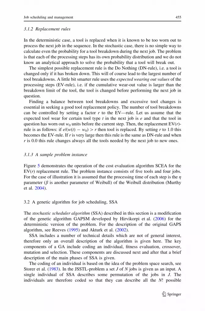
3.1.3 A sample problem instance

Figure 5 demonstrates the operation of the cost evaluation algorithm SCEA for the

EV(r) replacement rule. The problem instance consists of five tools and four jobs.

For the case of illustration it is assumed that the processing time of each step is the gparameter (b is another parameter of Weibull) of the Weibull distribution (Murthy

et al. 2004).

3.2 A genetic algorithm for job scheduling, SSA

The stochastic scheduler algorithm (SSA) described in this section is a modification

of the genetic algorithm GAPSM developed by Hirvikorpi et al. (2006) for the

deterministic version of the problem. For the description of the original GAPS

algorithm, see Reeves (1995) and Akturk et al. (2002).

SSA includes a number of technical details which are not of general interest,

therefore only an overall description of the algorithm is given here. The key

components of a GA include coding an individual, fitness evaluation, crossover,

mutation and selection. These components are discussed next and after that a brief

description of the main phases of SSA is given.

The coding of an individual is based on the idea of the problem space search, see

Storer et al. (1983). In the JSSTL-problem a set J of N jobs is given as an input. A

single individual of SSA describes some permutation of the jobs in J. The

individuals are therefore coded so that they can describe all the N! possible


123

permutations; an individual of the GA population is here expressed as a vector of

perturbation factors, which are real numbers from interval (0,1]. Each job in J is

associated with its perturbation factor which is used as a multiplier to the processing

time of the job in question. It is then possible to use a deterministic base heuristic to

calculate an order for the jobs from these perturbed processing times. The heuristic

Tool data:

Tools Wear-out limit w(t) Change time s(t)Tool 1 64 7 Tool 2 60 12 Tool 3 96 13 Tool 4 56 12 Tool 5 98 7

Job data:

Steps Job 1 Job 2 Job 3 Job 4Step 1 Tool 1 Tool 1 Tool 5 Tool 1β 1.073 1.028 1.026 1.074η 20.15 19.36 41.22 20.15Step 2 Tool 3 Tool 3 Tool 2 Tool 2β 0.799 0.966 1.063 0.764η 21.16 34.46 25.89 15.03Step 3 Tool 1 Tool 5 - Tool 3β 0.896 1.128 0.799η 18.90 15.65 21.16Step 4 Tool 4 - - - β 0.990η 20.24

Processing of the jobs: Job: 4 Add tool: 1Add tool: 2Add tool: 3Step 1 cost(1) : 21.274 ; the amount of wear on the first stepStep 2 cost(2) : 18.362 ; “” on the second stepStep 3 cost(3) : 26.582Job: 3 Add tool: 5Step 1 cost(5) : 45.105Step 2 cost(2) : 26.894 --> break-down -5.256725 ; tool wears more than five units over the wear-out limitStep 1 cost(5) : 45.467Step 2 cost(2) : 28.650Job: 2 Replace tool: 5 Step 1 cost(1) : 22.448Step 2 cost(3) : 40.556Step 3 cost(5) : 19.349Job: 1 Add tool: 3Replace tool: 1 Step 1 cost(1) : 23.290Step 2 cost(3) : 22.474Step 3 cost(1) : 22.587Step 4 cost(4) : 21.781

Fig. 5 A simple problem instance and the flow of a single simulation run with the stochastic costevaluation algorithm (SCEA). Magazine size is 3 tools and the jobs are processed in SPT-order (job 4, job3, job 2 and last job 1). In this flow the EV(1.2)-rule is used as the replacement rule and the removal ruleis SUM. The tool wear is modelled with Weibull distribution and the parameters for each step are given inthe job data. Symbols g and b are parameters of the Weibull distribution. The processing history includesone tool breakdown (tool 1, job 3) and in total 2 tool replacements


123

must be deterministic in the sense that when it is given certain processing times, it

produces always the same order. SSA uses the SPT-rule which sorts the jobs to an

order of increasing processing times. It is now easy to see that by choosing the

perturbation factors for the jobs properly, one can generate any of the permutations

of the jobs by applying the SPT-rule to these perturbed processing times. In this

way, an individual which is an ordering of the jobs is described fully by two

components: a perturbation vector and the fixed base heuristic.

The fitness of an individual is evaluated in two steps. In the first step SSA uses

the SPT-heuristic (our base heuristic) to create an ordered sequence of the jobs. The

processing times which have been perturbed (multiplied) with the perturbation

vector of the individual are used in this step. The result of the first step is then used

as an input to the cost evaluation algorithm SCEA. The result given by the cost

evaluation algorithm, which is an approximate of the average processing cost for the

given order, is the fitness of the individual (This is the major difference between

GAPSM and SSA, since GAPSM uses a deterministic cost evaluation algorithm due

to the different nature of the problem it solves).

In the crossover, parents are chosen by the tournament selection method. During

each tournament round candidate parents are selected randomly from the population

and compared against the current ones. The number of tournament rounds is

selected randomly from an interval which is given as a parameter. For example, if

the number of tournament rounds is 0 then the selection of the parents is purely

random. After the selection of the parents, the algorithm performs one-point

crossover by taking the first half of the perturbation factors from the other parent

and the rest from the other. These halves are then concatenated to form an offspring.

Each individual in the population is allowed to mutate with a small probability

during an iteration. When mutation event occurs, the algorithm selects one random

position in the perturbation vector of the individual in question and replaces it with

new random number from interval (0,1].

One offspring is created in a manner described earlier. This offspring then

replaces the worst individual in the current population (i.e. the individual with the

highest average processing cost). All the other individuals are directly transferred to

the next iteration.

The SSA algorithm begins by creating an initial population of certain size (given as

a parameter). This population is created purely random so that for each individual

every perturbation factor is chosen from a uniform distribution of (0,1]. In the

evolution phase SSA selects the individuals for the next generation through direct

transfer and crossover. After the selection, each individual of the next generation is

allowed to go through a mutation with a given probability (a parameter). The

evolution phase is repeated a predefined number of iterations and the result of the SSA

is the order described by the individual with the best fitness after the last iteration.

4 Empirical results

The number of tools and jobs varies greatly depending on the size of manufacturing

facility and the type of parts processed. For example a manufacturer producing large


123

engines may use a flexible machine for which the capacity of the tool magazine is

several hundreds of tools. In contrast to this, small workshops may have machines

for which the capacity of the tool magazine is less than 20 tools.

The data generation process first created the tool types. The maximum wear-out

value for tools was selected from a uniform distribution as well as the change time.

Once the tool types had been created, the process generated a large number of jobs.

For a job the number of steps is selected from uniform distribution. After this, the

process created a Weibull distribution for each tool-wearing step. The parameters of

this Weibull distribution (b and g) were taken from normal distributions, and the

processing step time was simply the expected value of the Weibull distribution. The

problem instances were created finally by selecting random jobs without replace-

ment from the large job set created earlier.

The selection of parameters for the data generation is a difficult task because

there is a certain realm in which the algorithms we presented are useful. For

example if the tool changes dominate over the job processing times then it is more

useful to minimize the number of tool changes. On the other hand if job processing

times dominate over the tool change times the SPT-rule will most likely be an

effective solution method. In Fig. 6 we give the parameters used in the data

generation.

4.1 Estimating the variance

In the first set of test runs we measured the standard deviation of the processing

costs when evaluated by SCEA. The primary objective was to find out how many

simulation runs are needed for small enough standard deviation (\1%). Another

objective was to determine how the problem size and replacement rule affect the

standard deviation. The results of these tests are summarized in Table 1 from which

Number of tool types: 50• Change time: UD(5, 15)• Wear out value: UD(40, 100)• Distribution: Weibull

Number of jobs: 200• Number of steps: UD(4,20) • Steps:

o Distribution: Weibull (depends on the tool type)β ND(1,0.2)η ND(0.3 * tool lifetime, 0.1)

Number of problem instances: 90 • Created with random sampling from the whole set of jobs:

o 1) 30 problem instances with 20 jobs;o 2) 30 instances with 60 jobs;o 3) 30 instances with 100 jobs

Fig. 6 Parameters of the test data generation process. In feasibility checks some of the jobs werereplaced because they did not fulfil the feasibility conditions 1 and 20 set for the problem instances


123

one can see that the standard deviation diminishes rapidly as the number of

simulation runs increases.

For small problem instances the number of simulation runs needed was greater

than for larger problem instances. One reason for this is that a single tool breakdown

in them causes larger proportional variation in the costs. Another observation is that

without any replacement rule (i.e. ‘‘change when breaks’’) the variance is large

because there are various tool breakdowns which makes the evaluated cost more

dependent on the random events. This must be taken into account when comparing

the replacement and removal rules.

4.2 Tuning the cost evaluation algorithm

In the second set of test runs the objective was to determine the best combination of

the removal/replacement rules for tool management and the parameters of this

combination. The best value for the r-parameter of the EV(r)-replacement rule was

searched first and after this, five different removal rules KTNS, KTWL,

HYBRID(0.5), SUM and TI were compared. The TI-rule has been proposed by

Turkcan et al. (2003) and it calculates the number of operations the tool can still

perform and multiplies it with the tool’s remaining lifetime.

Figure 7 shows for the EV(r)-rule the effect of the r-parameter on the average job

processing costs for the sample problems of Fig. 6. One can see that the optimal

value for both small and large problem instances is 0.8 for the EV(r)-rule. However,

one may not conclude that this value is best for all types of problem instances,

instead of that it should always be tuned for the particular problem type in question.

The shape of the curve in Fig. 7 can be explained as follows. Small r-values lead to

excessive number of tool replacements and large r to large number of tool

breakdowns. The optimal ‘‘risk’’ of tool breakdowns is somewhere between these

values. The problem size affects on how large proportional effect the excessive tool

changes have, i.e. for small problem instances the effect is larger as it can be seen

from Fig. 7 (r [ 1.3).

The combination of removal and replacement rules should work on all possible

orderings of the jobs and therefore we used 30 random sequences when determining

the best combination of these rules. From Table 2 one can see that the SUM-rule

Table 1 Standard deviation of the total processing costs using SCEA for DN and EV-replacement rules

Number of simulation

runs

20 jobs, DN

(%)

20 jobs, EV(0.5)

(%)

100 jobs, DN

(%)

100 jobs EV(0.5)

(%)

1 54 0.61 69 0.28

10 15 0.39 20 0.18

50 8.4 0.19 7.8 0.09

100 6.2 0.12 5.9 0.07

200 4.1 0.08 4.0 0.02

Standard deviation of processing cost is calculated from 30 cost evaluations for single problem instance.

The deviation is then normalized by the mean of the processing cost


123

was slightly better than the other removal rules. Surprisingly the KTWL-rule did not

perform very well. Also the TI-rule was significantly worse than the new SUM-rule.

4.3 Comparison of SSA against traditional methods

The results of SSA with the proposed stochastic cost evaluation algorithm were

compared against the SPT-rule. We also compared various rule combinations

against each other. The results in Table 3 show that the SSA with SCEA using the

new removal rules is significantly better than the previous methods.

Prop

ortio

nal p

roce

ssin

g co

st

0

0,5

1

1,5

2

2,5

3

3,5

0 0,5 1 1,5 2

20 jobs

60 jobs

100 jobs

r-value

Fig. 7 The effect of parameter r to the average processing cost. The average cost was estimated from 30random job sequences. Because these values are in different scale for different sized problems the valueswere calculated proportional to the EV(0.0)-value. The number of simulation runs was 200 and the toolremoval rule was random selection

Table 2 The effect of removal rules on the average processing cost

20 jobs 60 jobs 100 jobs

Best values Average-% Best values Average-% Best values Average-%

KTNS 2 0.00 2 0.00 2 0.00

KTWL 0 1.81 0 1.91 0 1.94

RANDOM 0 4.21 0 3.72 0 4.15

TI 0 1.71 0 1.31 0 1.67

SUM 28 -0.74 28 -0.72 28 -0.63

The average processing cost was calculated for 30 random job permutations and their results were

averaged. The ‘‘average-%’’ values are calculated as proportional difference to the KTNS-rule. ‘‘Best

values’’ give the number of times out of 30 tests the rule has found the best solution among the five rules


123

5 Conclusions

Stochastic scheduling and tool management were considered in this work. The

complexity of the problem prohibited us from using standard stochastic optimiza-

tion methods, like scenarios and analytical approaches. This complexity originated

from the recursive nature of the problem which requires, in a case of tool

breakdown, returning to the earlier stages of the processing. The feasibility and

optimality of the solutions were also discussed. We concluded that an accurate

feasibility check is difficult to do in a general case.

We proposed a cost evaluation algorithm which approximates the processing cost

as an average of several hundreds of realizations of the simulated manufacturing

process. The cost evaluation algorithm was parameterized for different removal and

replacement rules. The new tool removal rule, EV(r), turned out to be superior in

comparison to other rules tested here.

A genetic algorithm (SSA) was given for solving the stochastic scheduling and

tool management problem. The empirical tests indicate that SSA gives considerably

better results than processing with the traditional SPT-rule. The running times of

SSA were acceptable for practical applications.

The mathematical formulation of the JSSTL-problem is complex and it cannot be

solved with the existing optimization packages. Simplifying the problem to a form

which enables one to use traditional (i.e. analytical or scenario) approaches requires

more research. The cost function also includes only the time cost; material costs

incurring from discarded jobs are not yet included to the model. Taking these into

account requires the use of multi-objective optimization which would complicate

the situation even further.

Acknowledgement This work has been partially financed by the Graduate School, Turku Centre for

Computer Science (TUCS).

References

Adiri IJ, Bruno E, Frostig AHG, Rinnooy K (1989) Single machine flow-time scheduling with a single

breakdown. Acta Inform 26:679–696

Table 3 Comparison of the SPT-rule and the SSA-rule using different removal methods

20 jobs 60 jobs 100 jobs

Best Average Best Average Best Average

SPT(SUM, EV(0.8)) 3 62,440 2 536,900 8 1452,000

SPT(TI, EV(0.8)) 0 63,810 0 552,200 0 1512,000

SPT(KTWL,

EV(0.8))

0 65,100 0 552,600 0 1508,000

SSA(SUM, EV(0.8)) 21 61,490 21 526,500 21 1437,000

SSA(TI, EV(0.8)) 5 61,850 4 534,400 0 1467,000

SSA(KTWL,

EV(0.8))

1 63,240 3 534,700 1 1465,000


123

Ahmad M, Sheikh AK (1984) Berstein reliability model: derivation and estimation of parameters. Rel

Eng 8:131–148

Akturk MS, Ghosh JB, Gunes ED (2002) Scheduling with tool changes to minimize total completion

time: a study of heuristics and their performance. Naval Res Logist 50:15–30

Billatos SB, Kendall LAA (1991) General optimization model for multi-tool manufacturing systems.

Trans ASME 113(10):10–16

Birge JR, Louveaux F (1997) Introduction to stochastic programming. Springer Verlag

Crama Y, Kolen AWJ, Oerlemans AG, Spieksma FCR (1994) Minimizing the number of tool switches on

a flexible machine. Int J Flex Manuf Syst 6:33–53

Gibbs D, Crandell TM (1991) An introduction to CNC machining and programming. Industrial Press

Gray E, Seidmann A, Stecke KE (1993) A synthesis of decision models for tool management in

automated manufacturing. Manage Sci 39:549–567

Hirvikorpi M, Knuutila T, Nevalainen O (2006) Job ordering and management of wearing tools in flexible

manufacturing. Eng Optimiz 38(2):227–244

Iakovou E, Ip CM, Koulamas C (1996) Optimal solutions for the machining economics problem with

stochastically distributed tool lives. Eur J Oper Res 92(1):63–68

Iawata K, Murostu Y, Iwatsubo T, Fujii S (1972) A probabilistic approach to the determination of the

optimum cutting conditions. J Eng Ind Ser B 94(4):1099–1107

Jianqiang M, Keow LM (1997) Economical optimization of tool replacement intervals. Int Manuf Syst

8(1): 59–62

Knuutila T, Puranen M, Johnsson M, Nevalainen O (2001) Three perspectives for solving the job

grouping problem. Int J Prod Res 39(18):4261–4280

Lee CY, Liman SD (1992) Single machine flow-time scheduling with scheduled maintenance. Acta

Inform 29:375–382

Lee CY (1996) Machine scheduling with an availability constraint. J Glob Optim 9:395–416

Lee CY (1997) Minimizing the makespan in two-machine flowshop scheduling problem with an

availability constraint. Oper Res Lett 20:129–139

Murthy DNP, Xie M, Jiang R (2004) Weibull models. Wiley

Qi X, Chen T, Tu F (1999) Scheduling the maintenance on a single machine. J Oper Res Soc 50:1071–

1078

Reeves CR (1995) Modern heuristic techniques for combinatorial problems. McGraw-Hill International

Storer RH, Wu DS, Vaccari R (1983) New search spaces for sequencing problems with application to job

shop scheduling. Manage Sci 29:273–288

Tang CS, Denardo EV (1988) Models arising from a flexible manufacturing machine. Oper Res

36(5):767–784

Turkcan A, Akturk MS, Storer RH (2003) Non-identical parallel CNC machine scheduling. Int J Prod Res

41(10):2143–2168


123

Documents

Job scheduling and management of wearing tools with stochastic tool lifetimes