Interactions among vegetation and ozone, water and nitrogen fluxes in a coastal Mediterranean maquis ecosystem

BGD6, 1453–1495, 2009

Ozone, water andnitrogen fluxes in amaquis ecosystem

G. Gerosa et al.

Title Page

Abstract Introduction

Conclusions References

Tables Figures

J I

J I

Back Close

Full Screen / Esc

Printer-friendly Version

Interactive Discussion

Biogeosciences Discuss., 6, 1453–1495, 2009www.biogeosciences-discuss.net/6/1453/2009/© Author(s) 2009. This work is distributed underthe Creative Commons Attribution 3.0 License.

BiogeosciencesDiscussions

Biogeosciences Discussions is the access reviewed discussion forum of Biogeosciences

Interactions among vegetation and ozone,water and nitrogen fluxes in a coastalMediterranean maquis ecosystemG. Gerosa1, A. Finco1, S. Mereu3, R. Marzuoli2, and A. Ballarin-Denti1

1Dip.to di Matematica e Fisica, Universita Cattolica del S.C., via Musei 41, 25121 Brescia, Italy2CRINES, via Galilei 2, Curno, Italy3Dip.to di Biologia Vegetale, Universita La Sapienza, via Fermi 1, Roma, Italy

Received: 3 December 2008 – Accepted: 18 December 2008 – Published: 29 January 2009

Correspondence to: G. Gerosa ([email protected])

Published by Copernicus Publications on behalf of the European Geosciences Union.

1453

http://www.biogeosciences-discuss.net

http://www.biogeosciences-discuss.net/6/1453/2009/bgd-6-1453-2009-print.pdf

http://www.biogeosciences-discuss.net/6/1453/2009/bgd-6-1453-2009-discussion.html

http://creativecommons.org/licenses/by/3.0/

BGD6, 1453–1495, 2009


G. Gerosa et al.

Title Page



Tables Figures

J I

J I

Back Close

Full Screen / Esc



Abstract

Ozone, water and energy fluxes were measured over a Mediterranean maquis ecosys-tem from 5 May until 31 July by means of the eddy covariance technique. Additionalmeasurements of NOx fluxes were performed by the aerodynamic gradient technique.Stomatal ozone fluxes were obtained from water fluxes by a Dry Deposition Inferential5

Method based on a big leaf concept.The maquis ecosystem acted as a net sink for ozone. The different water availability

between late spring and summer was the major cause of the changes observed instomatal fluxes, which decreased, together with evapotranspiration, when the seasonbecame drier.10

NOx concentrations were significantly dependent on the local meteorology. NOxfluxes resulted less intense than the ozone fluxes. However an average upward flux ofboth NO and NO2 was measured.

The non-stomatal pathways of ozone deposition were investigated. A correlation ofnon-stomatal deposition with air humidity and, in a minor way, with NO2 fluxes was15

found.Ozone risk assessment was performed by comparing the exposure and the dose

metrics: AOT40 (Accumulated dose over a threshold of 40 ppb) and AFst1.6 (Accumu-lated stomatal flux of ozone over a threshold of 1.6 nmol m−2 s−1). AOT40, both at themeasurement height and at canopy height was greater than the Critical Level (500020

ppb·h) adopted by UN-ECE. Also the AFst1.6 value (12.6 mmol m−2 PLA, ProjectedLeaf Area) was higher than the provisional critical dose of 4 mmol m−2 PLA. The cumu-lated dose grew more regularly than the exposure but it showed two different growthrates in the spring and in the summer periods.

1454





BGD6, 1453–1495, 2009


G. Gerosa et al.

Title Page



Tables Figures

J I

J I

Back Close

Full Screen / Esc



1 Introduction

The toxicity of ozone for plants has been widely documented over the past twentyyears (Benton et al., 2000; Skarby et al., 1998). Once in the substomatal cavities ofthe leaves, ozone dissolves in the water film that covers the apoplast and sparks thegeneration of reactive oxygen species (ROS) which are considered to be responsible5

for biological damages (Baier et al., 2005; Iriti and Faoro, 2008, Heath, 2008) Amongthese injuries it is worth reminding the peroxidative destruction of membranes, theoxidation of the thiolic groups of proteins with a consequent alteration of enzymaticactivity, the degradation of chlorophylls and the interference with the electron transportsystems on which photosynthesis and respiration processes rely upon (Heath, 1996;10

Reichenauer et al., 1997; Bussotti et al., 2007a). These effects eventually lead to avisible damage on the leaf lamina (Bermejo et al., 2003; Novak et al., 2008; Marzuoliet al., 2008) Even if in most cases the effects remain latent they cause physiologicalalterations and a general loss in Net Primary Productivity (NPP) (Felzer et al., 2004;King et al., 2005).15

Mediterranean ecosystems, because of their climatic conditions and their proximityto anthropic sources of ozone precursors, are among the most exposed ecosystemsto this pollutant (Paoletti et al., 2006). The EMEP model estimated (Simpson et al.,2007) for the Mediterranean areas an exposure between 40 000 and 60 000 ppb·h (ona six months basis, April–September) for the year 2000, a value exceeding from 8 to20

12 times the critical level of 5000 ppb·h set by UN-ECE for the protection of forests andseminatural vegetation.

Nevertheless field observations never reported a particularly strong plant injury (Bus-sotti and Gerosa, 2002; Bussotti et al., 2006, Paoletti et al., 2006), thus questioningthe soundness of the exposure concept applied to ozone risk assessment. However,25

the lack of visible injuries in the Mediterranean vegetation could be due to extremelyefficient physiological and biochemical defense mechanisms of these plants to oxida-tive stress as some experiments in controlled environments revealed (Nali et al., 2004;Elvira et al., 2004).

1455





BGD6, 1453–1495, 2009


G. Gerosa et al.

Title Page



Tables Figures

J I

J I

Back Close

Full Screen / Esc



Among the physiological responses, stomatal regulation plays an important role. Fol-lowing the seasonal decrease of water availability typical of the Mediterranean summer,stomata close to reduce transpiration and water losses, thus limiting the dose of pol-lutant effectively absorbed and hence its effects. Because of the crucial role of stom-ata in regulating the dose absorption process, the cumulative ozone flux (AFstY) has5

been chosen by UN-ECE as a more reliable ozone risk index then AOT40 (Mussel-mann et al., 2006; Karlsson et al., 2007, Matyssek et al., 2007). This index is basedon the accumulation of stomatal fluxes over a threshold (Y) which accounts for thebiochemical detoxification mechanisms. This threshold value has been provisionallyset to 1.6 nmol m−2 s−1 (Karlsson et al., 2004) for forests and 6 nmol m−2 s−1 for crops10

(Pleijel et al., 2004), however the meaning and usefulness of Y is still debated anddiscussed in the UN-ECE effects-based community. Despite the acknowledged bet-ter biological soundness of AFstY over AOT40 (Matyssek et al., 2007, Karlsson et al.,2007) AOT40 is still widely used since field measurements of AFstY are difficult. Infact direct measurements of ozone flux can be performed only by micrometeorological15

techniques such as Eddy Covariance (EC) (Keronen et al., 2003), which requires theuse of not completely standardized complex equipment. As a consequence, flux basedrisk assessments is mostly performed with the aid of models, such as the depositionmodule DO3SE (Emberson et al., 2007; Ashmore et al., 2007) included in the EMEPmodel.20

Unfortunately, DO3SE has been validated mostly with observations of total O3 fluxand stomatal conductance (gs) in ecosystem types which are representative of theCentral and Northern Europe (e.g. Tuovinen et al., 2001). In Mediterranean conditionsonly one comparative study on wheat (Tuovinen et al., 2004) has been conducted inItaly and, to date, validation and comparison are still missing for an evergreen Mediter-25

ranean forest or the Mediterranean maquis. In fact it is important to test the model inconditions where high ozone concentrations can occur with high soil and atmosphericwater deficits (Emberson et al., 2005).

1456





BGD6, 1453–1495, 2009


G. Gerosa et al.

Title Page



Tables Figures

J I

J I

Back Close

Full Screen / Esc



This article is aimed to the analysis of the ozone flux dynamics and their interactionwith NOx in a water limited environment during the dry season, and to offer a datasetof measurements suitable for model calibration and validation. It is also aimed at as-sessing the ozone risk for a Mediterranean maquis ecosystem, by the measurement ofthe effective dose absorbed by the vegetation through stomata and its comparison with5

AOT40.

2 Materials and methods

Measurements were performed from 5 June to 31 July 2007 in a coastal Mediterraneanmaquis at Castelporziano, Italy. Details on the measuring site can be found in Fareset al. (2009). Two different techniques were used to measure turbulent fluxes of en-10

ergy and matter: the eddy covariance technique and the gradient approach. A DryDeposition Inferential Method approach (Wesely and Hicks, 2000; Gerosa et al., 2003,2005) was then applied to calculate the ozone stomatal fluxes and the toxicologicaldose absorbed by the ecosystem.

2.1 Instrumentation15

Sensible and latent heat fluxes as well as ozone fluxes were measured using theeddy covariance technique (Swinbank 1951; Hicks and Matt, 1988). An ultrasonicanemometer (USA-1, Metek, Elmshorn, Germany), a CO2/H2O open path fast sensor(LI-7500, LI-COR, Lincoln, Neb., USA) and a fast ozone analyser (COFA, Ecometrics,Italy) were mounted on the top of a 3.8 m tall scaffold.20

One net radiometer (NR lite, Kipp&Zonen, Holland), one PAR meter (190SA, LI-COR, Lincoln, Neb., USA) and a temperature and relative humidity probe (50Y, Camp-bell Scientific, Shepshed, United Kingdom) were placed at the same height than theanemometer.

An additional reference O3 analyzer (SIR S-5014, DASIBIE, Spain), sampling air at25

the top of the scaffold near the fast ozone sensor, was also used.1457





BGD6, 1453–1495, 2009


G. Gerosa et al.

Title Page



Tables Figures

J I

J I

Back Close

Full Screen / Esc



NO and NO2 fluxes were measured by a NOx analyzer (SIR 2308, DASIBIE, Spain)using the gradient approach, measuring the nitrogen oxides concentrations alterna-tively at two different heights by means of an electro-valve switching system controlledby a computer with a LabView (National Instruments, Austin, Tx, USA) software. Thetwo sampling points were chosen at 3.8 m and 1.3 m.5

The measuring site was equipped with additional instrumentation to better describethe temperature and humidity profile, the soil water status, the energy fluxes and themicroclimate of the area: two additional temperature and relative humidity probes (50Y,Campbell Scientific, Shepshed, United Kingdom) at 1 m and 0.1 m; three soil heat fluxplates, (HFP01SC, Hukseflux, Delft, Holland); three TDR reflectometers (C616, Camp-10

bell Scientific, Shepshed, United Kingdom); three leaf temperature probes (Pt100,DeltaT, United Kingdom); two surrogate leaves (237, Campbell Scientific, United King-dom) to measure leaf wetness, one rain gauge (52202, Young/Campbell Scientific,Cambridge, United Kingdom) and one barometer (PTB101B,Vaisala, Finland).

Fast sensors were sampled at 20 Hz by a computer with a customised software writ-15

ten in Delphi 5.0 (Borland). Slow sensors were sampled every 15 s and data werecollected by a datalogger (CR10x, Campbell Scientific, Shepshed, United Kingdom)equipped with a signal multiplexer device (AM16/32, Campbell Sci., United Kingdom),and data were averaged every 30 min.

2.2 Eddy-covariance20

Eddy covariance is a turbulence based technique which states that fluxes are equalto the covariance between the vertical component of the wind (w) and the measuredscalar quantity. Originally developed by Swinbank (1951), it has been accurately de-scribed and widely used for gas exchange measurements (e.g. Stull, 1988; Kaimal andFinnigan, 1994; Foken, 2008).25

Under some condition that have to be fulfilled (stationarity of the variables for whichvertical fluxes are calculated, horizontal homogeneity, absence of chemical sourcesand sinks between the measuring height and the exchanging surface, and average

1458





BGD6, 1453–1495, 2009


G. Gerosa et al.

Title Page



Tables Figures

J I

J I

Back Close

Full Screen / Esc



vertical wind component equal to zero; Grunhage et al., 2000) vertical fluxes are con-stant with height and ozone, sensible and latent heat fluxes can be calculated as follows

FO3= w ′C

′(1)

H = ρcpw ′T′

(2)

λE = λρw ′q′

(3)5

where C is the ozone concentration, T the air temperature, q the specific humidity ofthe air, ρ the air density, λ the constant of water vaporization, and cp the specific heat ofthe air. The primes (′) indicate fluctuations of each variable around their mean and theoverbars represent averages over a chosen time period, in our case a 30 min averagingperiod. This period is short enough to separate synoptic and diurnal variations from10

the turbulent data (van der Hoven, 1957), and long enough to include all turbulentfluctuations occurring in the atmospheric surface layer.

At the end of each 30 min averaging period, the fluctuations around the means werecalculated after linear detrending of the data series and a covariance matrix was cal-culated, i.e. the covariances between every considered parameter and each other.15

Then the covariance matrix was rotated following the three rotation suggested byMcMillen (1988) in order to eliminate the advective components resulting from smallnon-homogeneities of the exchanging surface and an eventual slight vertical tilt of theinstrumentation.

In order to ensure a perfect synchronization of the data series and to account for20

different instrumental delays, the data series of the variables acquired by fast sensorswere lagged with successive steps of 0.05 s, with respect to the wind data series,until the calculated fluxes reached their maximum value. When a maximum flux valuewas not found within the 60th lag, the sample was recognized as not stationary anddiscarded.25

1459





BGD6, 1453–1495, 2009


G. Gerosa et al.

Title Page



Tables Figures

J I

J I

Back Close

Full Screen / Esc



2.2.1 Data selection

In addition to the previous method, the fulfillment of the stationarity requirement hasbeen checked by using the selection criterion proposed by Dutaur et al. (1999). Thiscriterion requires that fluctuations are calculated in two different ways: as the differenceof the linear detrended series with the 30-min average, and as the difference with an5

instantaneous local running mean obtained by passing a mathematical R-C recursivefilter (analougous of an electric circuit of a resistor and a capacitor in series) over theoriginal time series.

If the normalized absolute difference between the covariances calculated with thefluctuations obtained with the two methods is below 1, the sample was considered as10

stationary and reliable. On the contrary, the sample was discarded.Other data selection criteria were that the data capturing efficiency of each sample

had to be greater than 85%, and that the canopy had to be completely dry. Only thedata that passed these selections were used for successive analysis.

2.2.2 Dry Deposition Inferential Method (resistive analysis)15

The deposition of a gas depends on many variables such as wind velocity, frictionvelocity, incoming radiation, temperature, surface type, etc. In the Dry Deposition Infer-ential Method approach (DDIM) the deposition surface is treated as a “big leaf” locatedat a height d+z0 over the soil, where d is the displacement height accounting for thecanopy height h (set to 2/3 of the h) and z0 is the roughness length which accounts20

for the canopy roughness. Three main phases are considered in the deposition pro-cess: first of all the gas must overcome the aerodynamic resistance (Ra) existing inthe turbulent layers of the atmosphere above the studied surface; then the gas mustmove across the quasi-laminar sub-layer which is characterized by a molecular diffu-sion against the so-called sub-laminar resistance (Rb); finally, in order to reach the25

surface, the gas must overcome the resistance of the surface itself (Rc). The deposi-tion flux of a gas is hence considered as the analogous of a current flowing through a

1460





BGD6, 1453–1495, 2009


G. Gerosa et al.

Title Page



Tables Figures

J I

J I

Back Close

Full Screen / Esc



electric circuit composed by these three resistances in series. Their equivalent resis-tance is called total resistance (Rtot) and it is equal to the concentration of the gas atthe measuring point divided by the flux:

Rtot = Ra + Rb + Rc = Czm/FO3(4)

The aerodynamic resistance Ra was calculated using the well known similarity rela-5

tion introduced by Monin and Obukhov (1954), while the sub-laminar resistance Rbfor ozone was calculated following the general purpose parameterization proposed byHicks et al. (1987). The surface resistance Rc is hence obtained as a residual sinceRtot is known, because it is derived from directly measured entities (Czm and FO3

).In order to estimate the fraction of gas penetrating through the stomata of plants, the10

surface resistance Rc (also called the canopy resistance in ecology) is broken downinto a stomatal resistance and a non-stomatal one mounted in parallel.

The stomatal resistance to ozone, RST , has been calculated from the stomatal resis-tance to water evaporation Rw by inverting the Penmann-Monteith equation (Monteith,1981) – i.e. by solving this equation for Rw since all the other entities are directly known15

from measurements – and by considering the relative diffusivity ratio of ozone in air tothat of water vapour.

The non-stomatal resistance was calculated as a residual from Rc and RST , followingthe rules of the parallel resistances.

The stomatal ozone flux was hence obtained as20

FST =Rc

(Ra + Rb + Rc)RSTCzm (5)

Further details can be found in Gerosa et al. (2005).The inferred resistances that showed values exceeding 10 000 s m−1 were rejected,

because of being unrealistic and causing numerical problems when used. The samehappened for samples where Rc resulted lower than 0 or RST was not computable25

because the Penman-Monteith equation could not be inverted.

1461





BGD6, 1453–1495, 2009


G. Gerosa et al.

Title Page



Tables Figures

J I

J I

Back Close

Full Screen / Esc



2.2.3 Ozone dose and exposure

In this work both exposure and dose approaches were compared. The exposure wascalculated as AOT40 for daylight hours only:

AOT40 =∑

∀GlobRad≥50W/m2

max(0;Cd+z0− 40)∆t (6)

where ∆t is the averaging period for the ozone concentration measurements (1 h).5

The concentration at d+z0, recommended by the ICP modelling and mapping manual(2004), was calculated with the Dry Deposition Inferential Method (Gerosa et al., 2005):

Cd+z0= Czm(1 − Ra/Rtot)

The ozone dose received by the ecosystem in the whole measuring period (May - July)was calculated as AFst0 by summing up all the 30-min ozone stomatal fluxes Fst of the10

period

AFst0 =∑

max(0; Fst)∆t (7)

where ∆t is the averaging period chosen for eddy covariance measurements.The dose was also calculated as AFst1.6:

AFst1.6 =∑

max(0; Fst − 1.6)∆t. (8)15

where Fst is the stomatal ozone flux obtained by the DDIM, 1.6 nmol m−2 s−1 is the UN-ECE detoxification threshold and ∆t is the averaging period of the flux measurements.

2.2.4 Data selection and data gap-filling

The results presented in this paper rely on the measured data that fulfilled all the selec-tion criteria. One unique exception has been made for the assessment of the exposure20

and the dose.1462





BGD6, 1453–1495, 2009


G. Gerosa et al.

Title Page



Tables Figures

J I

J I

Back Close

Full Screen / Esc



In fact, since both AOT40 and the ozone dose are cumulative metrics, a gap in ozoneconcentrations and ozone fluxes will result in an unavoidable underestimation of theirvalues.

To reduce such underestimation a gap-filling was performed. Gaps of no more than3 consecutive 30-min averages were linearly interpolated, while large gaps were gap-5

filled with time series reconstructed by multiple linear regression based on availablepredictors as local meteorological parameters and ozone concentrations from a nearbymeasuring station.

Gaps in stomatal fluxes could result also as a consequence from data rejection atthe output of the DDIM process. In these cases stomatal fluxes were estimated by10

taking the average stomatal fraction (the ratio between Fst and Ftot, based solely onmeasured data) at the corresponding half an hour, and by multiplying it by the availabletotal ozone flux .

2.3 Gradient approach

The aerodynamic gradient has been widely used to estimate surface fluxes (Grunhage15

et al., 2000; Foken, 2008) since, unlike eddy covariance, it does not require fast ana-lyzers. Here the turbulent diffusion coefficient for heat KH , that takes into account alsothe vertical stability of the atmosphere, was easily available from eddy covariance dataand applied to both nitric oxide and nitrogen dioxide fluxes, following the similarity ofthe transport of each scalar entity found by Monin and Obhukhov (1954) (Stull, 1988;20

Monteith and Unsworth, 1990; Pal Arya, 1988). Nitrogen oxides fluxes were hencecalculated for each semi-hour as follows:

FNOx= −KH ·∆[NOx]/∆z (9)

where NOx indicates alternatively NO and NO2, ∆[NOx] is the mean difference of NOand NO2concentrations between the two measuring heights z2 and z1, and ∆z is z2-z1,25

equal to 2.5 m in our case.

1463





BGD6, 1453–1495, 2009


G. Gerosa et al.

Title Page



Tables Figures

J I

J I

Back Close

Full Screen / Esc



3 Results

A total of 4176 semi-hourly samples were gathered during the whole measuring period.The samples referred to completely dry canopy conditions were 1894 (45.3%), becausenearly all the samples between 08:00 p.m. and 08:30 a.m. were excluded due to thepresence of dew on the leaves.5

This sub-dataset was further reduced by 16% because instrumental drawbacks (e.g.shut down, instrument breakings and substitutions), and by another 33.2% followingthe exclusion of the data which did not fulfill the stationarity conditions.

Hence the output of the DDIM analysis is based on the 50.8% of the data gatheredfrom 08:30 a.m. to 08:00 p.m., except when explicitly indicated.10

In order to highlight different meteorological and physiological traits, most of the re-sults are split in two different periods: the first one from 5 May to 12 June (late spring)and the second one from 13 June to 31 July (summer).

3.1 Ozone concentrations and fluxes

The average ozone concentration at the measuring height was 32.6 ppb in the first15

period and 38.6 ppb in the second one. The overall average was 35.9 ppb and themaximum peak concentration was 107 ppb. Ozone concentrations were strongly in-fluenced by the local meteorology: higher concentrations were observed when thewind was blowing from the sea and lower concentrations downwind to the city ofRome. Ozone concentrations usually began to increase early in the morning, around20

08:00 a.m. reaching their daily maximum in the first afternoon, and decreased to thelower nighttime values afterwards (Fig. 1). With the only exception of some days withhigh nighttime values, ozone concentrations showed a typical bell-shaped behavior.

On the contrary, the total ozone fluxes appear more irregular because of their intrin-sic link to the atmospheric turbulence. Substantial differences in the daily maximum25

absolute values (Fig. 1), which are usually reached in the first hours of the afternoon,are evident. A significant reduction of the average total ozone fluxes occurred in the

1464





BGD6, 1453–1495, 2009


G. Gerosa et al.

Title Page



Tables Figures

J I

J I

Back Close

Full Screen / Esc



second period: in the first period total fluxes were between 15 and 20 nmol m−2 s−1 fora large part of the day (08:00 a.m. to 07:00 p.m.), while in the second period they werearound 10 to 12 nmol m−2 s−1 (Fig. 2). Also nighttime values of the total fluxes wereslightly greater in the first period (about 7 nmol m−2 s−1) than the second one (about5 nmol m−2 s−1).5

The stomatal component of the ozone flux decreased as a consequence of stomatalresponse to a decreased water availability in the soil and an increased VPD in air(Mereu et al., 2009).

Figure 3 highlights the reduction in evapotranspiration that follows the decrease insoil water content (SWC hereafter). In the late spring the ecosystem could rely on a10

relatively high SWC, especially from the lower soil strata. In summer, the ecosystemexperienced dryer conditions, since water depletion involved the deeper soil layers andthe water table itself became shallower. Consequently, an increasing fraction of theavailable energy was thermically dissipated, while the fraction used for evapotranspira-tion decreased by more than 60%, from 105 W m−2 to 45 W m−2 in the central hours of15

the second period (Fig. 4).Also stomatal fluxes decreased their absolute diurnal mean value by 44% between

the first and the second period. Moreover their diurnal behavior changed too, as de-scribed in Fig. 2. In the first period ozone stomatal uptake showed a slight increasefrom the morning hours to the first hours of the afternoon (from 5 to 8 nmol m−2 s−1),20

and afterwards it decreased back to 5 nmol m−2 s−1 in the evening. In the second periodstomatal fluxes were about 4 nmol m−2 s−1 around 09:00 a.m. and slightly decreased toa constant value reached at midday (around 2.5 nmol m−2 s−1), then remained unvarieduntil sunset.

These stomatal fluxes were compared with the ozone stomatal uptake derived from25

sap flow measurements performed simultaneously on three species at the same site(Mereu et al., 2009) In Fig. 5 the sap flow uptake is obtained by summing up eachspecies uptake, upscaled by the species specific LAI and percentage cover as reportedby (Fares et al., 2009). The ozone flux attributed to these species shows a similar trend

1465





BGD6, 1453–1495, 2009


G. Gerosa et al.

Title Page



Tables Figures

J I

J I

Back Close

Full Screen / Esc



to that estimated from EC. In the first period, fluxes rapidly increased in the morninghours from values of less than 1 nmol m−2 s−1 to values of about 7 nmol m−2 s−1 around11:30 a.m. and gradually decrease afterwards. In the second period, the morning in-crement was significantly lower and fluxes reached a value of 2.5 nmol m−2 s−1 alreadyat 10:30 and remained steady for most of the day.5

As a consequence of the different water availability, the stomatal fraction of the ozoneflux absorbed by vegetation varied from a range of 40 to 50% of the total flux in the firstperiod, to a range of 20–30% in the second period. In the latter case, it is interesting tonote that the stomatal fraction was higher in the morning (45% around 09:00 a.m.), itrapidly decreased to a lower percentage for most of the day (Fig. 6 and slightly recov-10

ered to a 30% in the late afternoon.

3.2 Ozone exposure and dose

During the whole experimental period the ecosystem experienced an ozone exposure,expressed in terms of AOT40 for daylight hours of 20 650 ppb·h (Fig. 7). Such a valueis computed using ozone concentrations at zm=3.8 m a.s.l., but if it is computed with15

the concentrations at top canopy height, i.e. at d + z0, total exposure lowers to 8600ppb·h.

In the same period the stomatal dose, computed as a cumulative stomatal flux with-out any cutting threshold (AFst0), was 22.8 mmol m−2 PLA.

The exposure at zm during the measuring period shows an irregular growth which20

reflects the alternation of photochemical episodes with meteorological perturbations.The exposure at d + z0, after the initial increment between 20 May and 25 May, grewmore regularly due to the lower ozone concentrations at leaf level.

Dose development (AFst0), instead, was less variable, but a more careful analysisreveals two distinct periods with two different ozone assimilation rates, periods corre-25

sponding to late spring and summer (Fig. 7). In both periods the dose grew almostlinearly, at a rate of 0.17 mmol m−2 day−1 in the first period and of 0.11 mmol m−2 day−1

in the second. The two different rates clearly reflect the lower stomatal response in the1466





BGD6, 1453–1495, 2009


G. Gerosa et al.

Title Page



Tables Figures

J I

J I

Back Close

Full Screen / Esc



second period. Also AFst1.6 showed a similar trait, but with a lower growth rate duringsummer. The AFst1.6 dose at the end of the measured period was 12.6 mmol m−2 PLA,about the half of the AFst0 (55.3%).

3.3 Nitrogen oxides concentrations and fluxes

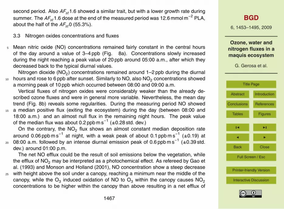
Mean nitric oxide (NO) concentrations remained fairly constant in the central hours5

of the day around a value of 3–4 ppb (Fig. 8a). Concentrations slowly increasedduring the night reaching a peak value of 20 ppb around 05:00 a.m., after which theydecreased back to the typical diurnal values.

Nitrogen dioxide (NO2) concentrations remained around 1–2 ppb during the diurnalhours and rose to 6 ppb after sunset. Similarly to NO, also NO2 concentrations showed10

a morning peak of 10 ppb which occurred between 08:00 and 09:00 a.m.Vertical fluxes of nitrogen oxides were considerably weaker than the already de-

scribed ozone fluxes and were in general more variable. Nevertheless, the mean daytrend (Fig. 8b) reveals some regularities. During the measuring period NO showeda median positive flux (exiting the ecosystem) during the day (between 08:00 and15

18:00 a.m.) and an almost null flux in the remaining night hours. The peak valueof the median flux was about 0.2 ppb m s−1 (±0.28 std. dev.)

On the contrary, the NO2 flux shows an almost constant median deposition ratearound 0.06 ppb m s−1 at night, with a weak peak of about 0.1 ppb m s−1 (±0.19) at08:00 a.m. followed by an intense diurnal emission peak of 0.6 ppb m s−1 (±0.39 std.20

dev.) around 01:00 p.m.The net NO efflux could be the result of soil emissions below the vegetation, while

the efflux of NO2 may be interpreted as a photochemical effect. As refereed by Gao etal. (1993) and Monson and Holland (2001), NO concentration show a steep decreasewith height above the soil under a canopy, reaching a minimum near the middle of the25

canopy, while the O3 induced oxidation of NO to O3 within the canopy causes NO2concentrations to be higher within the canopy than above resulting in a net efflux of

1467





BGD6, 1453–1495, 2009


G. Gerosa et al.

Title Page



Tables Figures

J I

J I

Back Close

Full Screen / Esc



NO2. The origin of such imbalance is not completely clear and could be attributed toadvection, deposition and transformation by nighttime chemistry of nitrogen speciestransported from Rome by the city plume.

4 Discussion

The order of magnitude of the ozone dose received by the maquis ecosystem is compa-5

rable to the dose received by the Holm Oak forest positioned just 0.8 km inland (Gerosaet al., 2008a) and it is also similar to the amount absorbed by barley and wheat crops(Gerosa et al., 2003, 2005). Apparently, the dose does not vary greatly despite theevident structural differences of these ecosystems and the different leaf and canopystomatal conductance. In all these cases, only a small portion of the ozone received10

by the ecosystem is effectively absorbed by the stomata. The greatest part of ozone,instead, is depleted in chemical-physical processes that altogether are termed non-stomatal deposition

4.1 Stomatal uptake

It is important to notice that night time hours are frequently characterized by thermal15

inversions, which determine the accumulation of dew over the canopy and soil (Ciesliket al., 2009; Mereu et al., 2009). The formation of dew between 02:00 and 06:00 a.m.,as well as the immediate drying of the leaf lamina and the evaporation of dew immedi-ately after 06:00 a.m., are confirmed by the leaf wetness sensors (Fig. 9). When thisevent takes place, the morning flux due to evaporation from the stand surfaces could20

be erroneously attributed solely to a stomatal activity. It is for this reason that the pre-sented results were filtered in order to exclude fluxes measured when the canopy waswet or in the following hour. However it cannot be excluded that the evaporation of dewhides a prominent stomatal opening (Fig. 10). In fact, light intensity is sufficient to cuestomatal aperture already from the first hours of the morning (PPFD at 07:00 a.m. was25

1468





BGD6, 1453–1495, 2009


G. Gerosa et al.

Title Page



Tables Figures

J I

J I

Back Close

Full Screen / Esc



around 300µE m−2 s−1) and it could be that after the evaporation of dew and as theVPD increases, guard cells adjust in order to reduce gs to the lower values of the day.

However, the sap flux measurements performed on three species, (Mereu et al.,2009) contradict this hypothesis. With the only exception of the driest period (late July),sap flux showed a bell shaped trend and a peak in sap flux never occurred in the morn-5

ing (Fig. 11). However, the measured species only represent 38% of the total cover(Fares et al., 2009), hence if a morning transpiration peak is really taking place, it couldbe attributed to the other species. But this eventuality has to be excluded by the factthat also the unmeasured species (Q. ilex, P. latifolia, C. incanus) are known to behavein a similar way for the transpiration rate (Bombelli and Gratani, 2003). The only ex-10

ception could be Rosmarinus officinalis (17% of the cover), but the SWC (Ψs<−1 MPa)was low enough to ensure a reduction of its stomatal conductance of more than 80%(Clary et al., 2004). It is hence most likely that the observed morning peak is an artifactattributable simply to dew evaporation.

This underline the importance of verifying dry canopy conditions in EC based flux15

measurements, even in xeric environments, and the potential advantage of couplingEC measurements with sap flow gauges.

4.2 Non-stomatal deposition

The nature of the non-stomatal deposition (Fnstom), more than 50% percent in this study,is still not understood and different hypothesis have been made to explain it. Van20

Pul and Jacobs (1994), after observing that the Fnstom increased with the efficiencyof ozone transport inside the canopy, suggested the cause to be the destruction ofozone over the plant and soil surfaces, since they observed that the ozone transportefficiency is proportional to u∗ and inversely related to the Leaf Area Index (LAI) andto the vegetation height. Instead, in a laboratory experiment Rondon (1993) showed25

that cuticular uptake by leaf waxes increased from a negligible rate at low levels oflight intensity, to rates comparable with stomatal uptake at light levels equivalent tostrong sunlight conditions, thus suggesting an important role of solar radiation. Fowler

1469





BGD6, 1453–1495, 2009


G. Gerosa et al.

Title Page



Tables Figures

J I

J I

Back Close

Full Screen / Esc



et al. (2001) suggested that the relationship between Fnstom and radiation reportedby Rondon (1993) and by Coe et al. (1995) could be explained as thermal decompo-sition of the ozone molecules intercepting the surfaces heated by radiation; they alsoestimated the energy of activation of this reaction to be 36 KJ mol−1. Kurpius and Gold-stein (2003), instead, observed that the exponential form of the relationship between5

Fnstom and temperature was similar to the relationship between temperature and theemission rate of Volatile Organic Compounds (VOC). Based on this similarity, they ad-vanced the hypothesis the a great fraction of the daytime ozone deposition could be aconsequence of gas-phase reactions with biogenic hydrocarbons and estimated that45 to 55% of the total ozone flux could depend on such reactions. However Mikkelsen10

et al. (2000) estimated from concurrently measured α- and β-pinene fluxes a maximumdestruction potential of monoterpene emissions corresponding only to 10% of the totalozone flux.

A role in non-stomatal ozone depletion has been also attributed to gas-phase tri-tration reactions with biogenic emissions of NO. The measurements of Dorsey et15

al. (2004) and of Pilegaard et al. (1999), and the precedent models of Duyzer etal. (1995) and Walton et al. (1997), highlighted that NO emissions from forest soilsnot only affect the magnitude and the direction of the NO2 fluxes, but also the intensityof ozone fluxes. Nevertheless, the influence on the latter is usually weak, but not negli-gible, and can become relevant in case of a high soil NO efflux (Pilegaard et al., 1999),20

when a substantial (∼30%) amount of the total ozone flux could be accounted for bychemical reactions, especially at night (Pilegaard, 2001; Walton et al., 1997). Finally,Altimir et al. (2004) found an influence of the atmospheric humidity on non-stomataldeposition at night, with an hyperbolic increase of surface conductance to ozone withsaturating RH %.25

In this study, the analysis of the data presented in Fig. 12 allow to support only thehypothesis of a direct influence of atmospheric humidity on non-stomatal deposition. Agas-phase reaction with NO of biogenic and antropic origin could be observed but onlyat high efflux rates as reported by Pilegaard et al. (1999).

1470





BGD6, 1453–1495, 2009


G. Gerosa et al.

Title Page



Tables Figures

J I

J I

Back Close

Full Screen / Esc



The occurrence of this reaction is revealed by the hyperbolic dependence (R2=0.95)of Fnstom on the NO2 fluxes observed over the canopy (Fig. 12f).

The dependence on RH, instead, is revealed by the median values of non-stomatalconductance, that, increased linearly together with the absolute humidity of air(R2=0.63) when the canopy wais completely dry (Fig. 12d). When the canopy was5

wet (mostly at night in our site) the relationship became hyperbolic (R2=0.60) (Fig. 13)as already found by Altimir et al. (2004). In this last case, ozone is not only removed byreactions with atmospheric water, but also dissolved in the water film deposited overthe colder surfaces, i.e. leaves, stems and soil. The chemical process of ozone decom-position and reaction with air water vapour and droplets has been described by Seinfeld10

and Pandis (1997) and de Paula and Atkins (2006). Nevertheless, the proximity of thecoastline could bring to suppose a contribution of marine aerosols which can modifythe chemical properties of the water films and consequently enhance ozone solubilityand its removal. Recent findings on the chemistry of halogen compounds (Br, I, Cl)in marine boundary layers MBL (Monks, 2005), suggest a possible role of these gas15

compounds in the removal of ozone in our coastal site. In fact, bromine and chlorine inthe MBL are emitted through the production of sea salt aerosol, with a smaller fractionreleased from biogenic organic halogens. Iodine compounds on the other hand arelargely released as organic compounds and molecular iodine from micro and macroalgae that accumulate iodine from the sea water (von Glasow, 2008). Chemical and20

photochemical reactions rapidly convert these compounds in halogenated monoxides(Monks, 2005). It is these latter compounds that are directly responsible for the catalyticremoval through one principal and simple mechanism (von Glasow et al., 2002):

XO + YO → X + Y + O2 with X and Y=Br, I,Cl (10)

X + O3 → XO + O2 (11)25

Model calculations have indicated that the presence of only 0.5–4 pmol mol−1 BrOcan significantly impact the O3 budget in the MBL (von Glasow et al., 2002; von Glasowand Crutzen, 2004).

1471





BGD6, 1453–1495, 2009


G. Gerosa et al.

Title Page



Tables Figures

J I

J I

Back Close

Full Screen / Esc



Recently, BrO and IO measurements in Green Cape, not only confirmed the occur-rence of such mechanism but also brought to the conclusion that the ozone photo-chemistry is largely dominated by halogen chemistry (Read et al., 2008). Interestingly,the daily profile reported for BrO and IO concentrations is similar to the ozone depo-sition found in this study. Concentrations of both gasses reach a maximum around5

10:00 a.m., remain constant until 14:00 p.m. for IO and until 07:00 p.m. for BrO, anddecrease to 0 afterwards. In the coastal site subject to a considerable external sourceof NOx at night, as in this case, the formation of halogenated nitrates – as BrONO2 –can take place. At sunrise, these compounds photolyse freeing NO2 and halogenatedoxides that may trigger and amplify the catalytic destruction of ozone. Such a process10

is what is suggested by the so-called “sunrise ozone destruction” reported by differentauthors (Nagao et al., 1999, Galbally et al., 2000, Watanabe et al., 2005). Such amorning peak of ozone depletion was already reported for a close site (Gerosa et al.,2005, 2008) and it occurred again during this campaign. The morning peak, especiallyin the first period, can be inferred from Figs. 2 and 6, where a rise in total ozone depo-15

sition is not supported by a concomitant rise in ozone stomatal uptake. This hypothesiswould also explain the NO2 efflux in excess observed in the maquis during the day. Infact, the air masses of the city plume rich in nitrate species, would first be transportedoffshore from the night breeze and return to land during the day under the form of or-ganic and halogenated nitrous compounds. Hence, if the hypothesis of the role of the20

chemistry of halogenated compounds should be confirmed also for this site, the corre-lation found with humidity could simply be an indicator of the transport of halogenatedspecies from the sea when the wind was blowing from offshore.

4.3 Ozone risk assessment

Ozone exposure was calculated as AOT40 using ozone concentrations both at the25

measuring point and at canopy level, calculating the latter ones by means of the DDIM.In both cases the ozone exposure exceeded the critical level (CL) of 5000 ppb·h

established for plants protection, revealing a potentially ozone hazard condition for the1472





BGD6, 1453–1495, 2009


G. Gerosa et al.

Title Page



Tables Figures

J I

J I

Back Close

Full Screen / Esc



maquis ecosystem. Considering that the vegetative period of maquis is much longerthan our measuring period, it can be reasonably supposed that the exposure to whichthese ecosystems are usually subject to is very high.

It is worth noticing that the CL was exceeded very soon by the AOT40 evaluated atthe measuring height (23 May), and only one month and half later (5 July) at the canopy5

height d+z0. The two metrics gave very different results, highlighting the importanceof following the indications of the Mapping Manual (ICP Modelling and Mapping, 2004),the disrespect of which may bring to considerable overestimation of the risks – a threefold higher in this case – and to erroneous conclusions. The risk of overestimating thenegative effects of ozone on the vegetation is particularly high in the Mediterranean10

area, where the concentrations of this pollutant are usually high (Paoletti, 2006).The failure to estimate ozone concentrations at top canopy height is not necessarily

due to negligence, but to the lack of the necessary information to infer the ozone gradi-ent above the canopy when using data from monitoring network stations, which usuallysample at a height of 3m. The determination of such gradient, in fact, requires knowl-15

edge of the aerodynamic state of the atmospheric surface layer (turbulence/stability)and the conductance to ozone of the ecosystem, which is known to vary rapidly as aresponse to the environmental conditions and to the physiological state of the plant.Ultimately, ozone exposure at top canopy height can be determined only through directflux measurements. Measurements that, as in this case, can be more profitably used20

to determine the stomatal ozone uptake, the only toxicological significant parameter.The dose of ozone absorbed by the vegetation during the measuring period, appears

well above the provisional critical flux level of 4 mmol m−2, expressed as AFst1.6, for thereduction of 5% of biomass growing in beech and birch (ICP Modelling and Mapping,2004; Karlsson et al., 2004)25

This dose, however, is below the critical dose for the appearance of visible injurysymptoms on leaves (30 mmol m−2 ) of beech and poplar found in recent OTC exper-iments (Gerosa et al., 2008b). These experiments reported also that even at lowerdoses, even asymptomatic species such as Q. robur showed a marked reduction in

1473





BGD6, 1453–1495, 2009


G. Gerosa et al.

Title Page



Tables Figures

J I

J I

Back Close

Full Screen / Esc



the photosynthetic efficiency (Bussotti et al., 2007). So, even if leaf injuries were notreported in this study, it cannot be excluded that photosynthetic assimilation was nega-tively influenced by ozone and ozone activated antioxidant systems capable of protect-ing the vegetation from photo-oxidative stress (Nali et al., 2004; Paoletti, 2006).

In any case, in a multi specific ecosystem the ozone risk assessment might to be5

more precise and take into account the specific physiology of each specie. Somespecies, in fact, can largely account for the dose of ozone absorbed by the ecosystemand hence may be relatively more effected by this pollutant and trigger future changesin ecosystem composition. This is what happened, for example, for the three speciesA. unedo, Q. ilex, E. arborea considered in drawing the Fig. 4.10

Finally, the measured dose is very close to the 24 mmol m−2 estimated for genericforests, in the same area and for the year 2000, by the renovated deposition moduleDO3SE-EMEP (Simpson et al., 2007). But it should be noted that the model estimationcovered 6 months of the entire growing season and not only the central three months,as in our case.15

In any case model parameterizations for this ecosystem are still necessary.

5 Conclusions

The maquis ecosystem acted as a net sink for ozone and the ozone deposition wasquite high. Nevertheless, only a minor part of the ozone flux (32.8%) was absorbed byvegetation through the stomata. The stomatal uptake was influenced by water avail-20

ability and decreased throughout the measuring period as the season became dryer.The remaining part of the ozone deposition, the so called non-stomatal one, was

positively influenced by air humidity and by nitrogen oxides. Nevertheless the influenceof these latter was weak, and was evident only when nitrogen fluxes were particularlyhigh. No influence with other measured factors, such as temperature, solar radiation25

and turbulence intensity were found. Moreover, due to the coastal location of the mea-suring site, a possible role on ozone depletion of halogenated species avvected from

1474





BGD6, 1453–1495, 2009


G. Gerosa et al.

Title Page



Tables Figures

J I

J I

Back Close

Full Screen / Esc



the sea was also suggested as a working hypothesis, even if it should be confirmed bynew measurements.

The maquis ecosystem resulted at high risk for ozone considering both AOT40and AFst1.6 approaches, just on a three months base instead of six months as sug-gested by UN-ECE. Hence, negative effects on the vegetation community cannot be ex-5

cluded for this particular ecosystem, and more in general for the Mediterranean maquisecosystems. However the different behaviors shown by the exposure and the dosemetrics highlighted the need for field measurements in order to realize a better riskassessment.

Finally a significant dataset is now available for testing, refining and validating depo-10

sition models on this type of ecosystems and Mediterranean climatic conditions

Acknowledgements. The field campaign was supported by the VOCBAS and AC-CENT/BIAFLUX programs. We’re also grateful to the Exchange of Staff funding Program ofthe ACCENT/BIAFLUX Network of Excellence for its support.

A special thank to the Scientific Committee of the Presidential Estate of Castelporziano and to15

its staff who allowed this work.

References

Altimir, N., Tuovinen, J., Vesala, T., Kulmala, M., and Hari, P.: Measurements of ozone removalby Scots pine shoots: calibration of a stomatal uptake model including the non-stomatalcomponent, Atmos. Environ., 38, 2387–2398, 2004.20

Ashmore, M., Buker, P., Emberson, L., Terry, A. C., and Toet, S.: Modelling stomatal ozoneflux and deposition to grassland communities across Europe, Environ. Pollut., 146, 659–670,2007.

Baier, M., Kandlbinder, A., Golldack, D., and Dietz, K. J.: Oxidative stress and ozone: percep-tion, signalling and response, Plant Cell Environ., 28, 1012–1020, 2005.25

Benton, J., Fuhrer, J., Gimeno, B. S., Skarby, L., Palmer-Brown, D., Ball, G. R., Roadknight, C.,and Mills, G.: An international cooperative programme indicates the widespread occurrenceof ozone injury on crops, Agr. Ecosyst. Environ., 78, 19–30, 2000.

1475





BGD6, 1453–1495, 2009


G. Gerosa et al.

Title Page



Tables Figures

J I

J I

Back Close

Full Screen / Esc



Bermejo, V., Gimeno, B. S., Sanz, M. J., De La Torre, D., and Gil, J. M.: Assessment of theozone sensitivity of 22 native plant species from Mediterranean annual pastures based onvisible injury, Atmos. Environ., 37, 4667–4677, 2003.

Bussotti, F. and Gerosa, G.: Are the Mediterranean forests in Southern Europe threatened fromozone?, J. Medit. Ecol., 3, 23–34, 2002.5

Bombelli, A. and Gratani, L.: Interspecific Differences of Leaf Gas Exchange and Water Re-lations of Three Evergreen Mediterranean Shrub Species, Photosynthetica, 41, 619–625,2003.

Bussotti, F., Cozzi, A., and Ferretti, M.: Field Surveys of Ozone Symptoms on SpontaneousVegetation. Limitations and Potentialities of the European programme, Environ. Monit. As-10

sess., 115, 335–348, 2006.Bussotti, F., Strasser, R. J., and Schaub, M.: Photosynthetic behavior of woody species under

high ozone exposure probed with the JIP-test: A review, Environ. Pollut., 147, 430–437,2007a.

Bussotti, F., Desotgiu, R., Cascio, C., Strasser, R. J., Gerosa, G., and Marzuoli, R.: Photo-15

synthesis responses to ozone in young trees of three species with different sensitivities, ina 2-year open-top chamber experiment (Curno, Italy), Physiol. Plantarum, 130, 122–135,2007b.

Cieslik, S., Gerosa, G., Finco, A., Cape, N., Misztal, P., and Matteucci, G.: Turbulence ina coastal Mediterranean area: Surface fluxes and related parameters at Castel Porziano,20

Biogeosciences Discuss., accepted, 2009.Clary, J., Save, R., Biel, C., and Herralde, F.: Water relations in competitive interactions of

Mediterranean grasses and shrubs, Ann. Appl. Biol., 144, 149–155, 2004.Coe, H., Gallagher, M., Choularton, T., and Dore, C.: Canopy scale measurements of stomatal

and cuticular O∼3 uptake by Sitka Spruce, Atmos. Environ., 29, 1413–1413, 1995.25

De Paula, J. and Atkins, P.: Explorations in Physical Chemistry, Oxford University Press, 2006.Dorsey, J. R., Duyzer, J. H., Gallagher, M. W., Coe, H., Pilegaard, K., Weststrate, J. H., Jensen,

N. O., and Walton, S.: Oxidized nitrogen and ozone interaction with forests. I: Experimentalobservations and analysis of exchange with Douglas fir, Q. J. Roy. Meteor. Soc., 130, 1941–1955, 2004.30

Dutaur, L., Carrara, S., and Lopez, A.: The detection of nonstationarity in the determination ofdeposition fluxes, Proceedings of EUROTRAC Symposium’98, 171–176, 1999.

1476





BGD6, 1453–1495, 2009


G. Gerosa et al.

Title Page



Tables Figures

J I

J I

Back Close

Full Screen / Esc



Duyzer, J., Weststrate, H., and Walton, S.: Exchange of ozone and nitrogen oxides betweenthe atmosphere and coniferous forest, Water Air Soil Poll., 85, 2065–2070, 1995.

Elvira, S., Bermejo, V., Manrique, E., and Gimeno, B. S.: On the response of two populationsof Quercus coccifera to ozone and its relationship with ozone uptake, Atmos. Environ., 38,2305–2311, 2004.5

Emberson, L., Buker, P., and Ashmore, M.: Assessing the risk caused by ground level ozone toEuropean forest trees: A case study in pine, beech and oak across different climate regions,Environ. Pollut., 147, 454–466, 2007.

Emberson, L. D., Massman, W. J., Buker, P., Soja, G., van de Sand, I., Mills, G., and Jacobs,C.: The development, evaluation and application of O 3 flux and flux-response models for10

additional agricultural crops, Critical Levels for Ozone: Further Applying and Developing theFlux-based Concept, Innsbruck, Austria, 2005.

Fares, S., Mereu, S., Scarascia Mugnozza, G., Vitale, M., Frattoni, M., Ciccioli, P., Tinelli, A.,and Loreto, F.: The ACCENT-VOCBAS field campaign on biosphere-atmosphere interactionsin a Mediterranean ecosystem of Castelporziano (Rome): site characteristics, climatic and15

meteorological conditions, and eco-physiology of vegetation, Biogeosciences Discuss., 6,1185–1227, 2009,http://www.biogeosciences-discuss.net/6/1185/2009/.

Felzer, B., Kicklighter, D., Melillo, J., Wang, C., Zhuang, Q., and Prinn, R.: Effects of ozone onnet primary production and carbon sequestration in the conterminous United States using a20

biogeochemistry model, Tellus B, 56, 230–248, 2004.Foken, T.: Micrometeorology, Springer, 2008.Fowler, D., Flechard, C., Cape, J. N., Storeton-West, R. L., and Coyle, M.: Measurements

of Ozone Deposition to Vegetation Quantifying the Flux, the Stomatal and Non-StomatalComponents, Water Air Soil Poll., 130, 63–74, 2001.25

Galbally, I. E., Bentley, S. T., and Meyer, C. P. M.: Mid-latitude marine boundary-layer ozonedestruction at visible sunrise observed at Cape Grim, Tasmania, 41 S, Geophys. Res. Lett.,27, 3841–3844, 2000.

Gao, W., Wesely, M., and Doskey, P.: Numerical modeling of the turbulent diffusion and chem-istry of NO x, O 3, isoprene, and other reactive trace gases in and above a forest canopy, J.30

Geophys. Res., 98, 18 339–18 354, 1993.

1477





http://www.biogeosciences-discuss.net/6/1185/2009/

BGD6, 1453–1495, 2009


G. Gerosa et al.

Title Page



Tables Figures

J I

J I

Back Close

Full Screen / Esc



Gerosa, G., Cieslik, S., and Ballarin-Denti, A.: Micrometeorological determination of time-integrated stomatal ozone fluxes over wheat: a case study in Northern Italy, Atmos. Environ.,37, 777–788, 2003.

Gerosa, G., Marzuoli, R., Cieslik, S., and Ballarin-Denti, A.: Stomatal ozone fluxes over abarley field in Italy. “Effective exposure” as a possible link between exposure-and flux-based5

approaches, Atmos. Environ., 38, 2421–2432, 2004.Gerosa, G., Vitale, M., Finco, A., Manes, F., Ballarin-Denti, A., and Cieslik, S. A.: Ozone uptake

by an evergreen Mediterranean Forest (Quercus ilex) in Italy. Part I: Micrometeorological fluxmeasurements and flux partitioning, Atmos. Environ., 39, 3255–3266, 2005.

Gerosa, G., Finco, A., Mereu, S., Vitale, M., Manes, F., and Ballarin Denti, A.: Com-10

parison of seasonal variations of ozone exposure and fluxes in a Mediterranean Holmoak forest between the exceptionally dry 2003 and the following year, Environ. Pollut.,doi:10.1016/j.envpol.2007.11.025, in press, 2008a.

Gerosa, G., Marzuoli, R., Desotgiu, R., Bussotti, F., and Ballarin-Denti, A.: Validation of thestomatal flux approach for the assessment of ozone effects on young forest trees. A sum-15

mary report of the TOP (Transboundary Ozone Pollution) experiment at Curno, Italy, Environ.Pollut., doi:10.1016/j.envpol.2008.09.042, in press, 2008b.

Grunhage, L., Haenel, H., and Jager, H.: The exchange of ozone between vegetation andatmosphere: micrometeorological measurement techniques and models, Environ. Pollut.,109, 373–392, 2000.20

Heath, R. L.: The modification of photosynthetic capacity induced by ozone exposure, Photo-synthesis and the Environment, Kluwer Academic Publishers, Dordrecht, 409–433, 1996.

Heath, R. L.: Modification of the biochemical pathways of plants induced by ozone: What arethe varied routes to change?, Environ. Pollut., 2008.

Hicks, B., Baldocchi, D., Meyers, T., Hosker, R., and Matt, D.: A preliminary multiple resistance25

routine for deriving dry deposition velocities from measured quantities, Water Air Soil Poll.,36, 311–330, 1987.

Hicks, B. B. and Matt, D. R.: Combining biology, chemistry, and meteorology in modeling andmeasuring dry deposition, J. Atmos. Chem., 6, 117–131, 1988.

ICP Modelling and Mapping: Manual on Methodologies and Criteria for Modelling and Mapping30

Critical Loads and Levels and Air Pollution Effects, Risks and Trends, Federal EnvironmentalAgency (Umweltbundesamt), Berlin, UBA-Texte52/04, www.icpmapping.org, 2004.

1478





www.icpmapping.org

BGD6, 1453–1495, 2009


G. Gerosa et al.

Title Page



Tables Figures

J I

J I

Back Close

Full Screen / Esc



Iriti, M. and Faoro, F.: Oxidative Stress, the Paradigm of Ozone Toxicity in Plants and Animals,Water Air Soil Poll., 187, 285–301, 2008.

Kaimal, J. and Finnigan, J.: Atmospheric Boundary Layer Flows: Their Structure and Measure-ment, Oxford University Press, USA, 1994.

Karlsson, P. E., Braun, S., Broadmeadow, M., Elvira, S., Emberson, L., Gimeno, B., Thiec, D. L.,5

Novak, K., Oksanen, E., Schaub, M., Uddling, J., and Wilkinson, M.: Risk assessments forforest trees: The performance of the ozone flux versus the AOT concepts, Environ. Pollut.,146, 608–616, 2007.

Karlsson, P., Uddling, J., Braun, S., Broadmeadow, M., Elvira, S., Gimeno, B., Le Thiec, D.,Oksanen, E., Vandermeiren, K., and Wilkinson, M.: New critical levels for ozone effects10

on young trees based on AOT40 and simulated cumulative leaf uptake of ozone, Atmos.Environ., 38, 2283–2294, 2004.

Keronen, P., Reissell, A., Rannik, U., Pohja, T., Siivola, E., Hiltunen, V., Hari, P., Kulmala, M.,and Vesala, T.: Ozone flux measurements over a Scots pine forest using eddy covariancemethod: performance evaluation and comparison with flux-profile method, Boreal Environ.15

Res., 8, 425-444, 2003.King, J. S., Kubiske, M. E., Pregitzer, K. S., Hendrey, G. R., McDonald, E. P., Giardina, C. P.,

Quinn, V. S., and Karnosky, D. F.: Tropospheric O3 compromises net primary productionin young stands of trembling aspen, paper birch and sugar maple in response to elevatedatmospheric CO2, New Phytol., 168, 623–636, 2005.20

Kurpius, M. and Goldstein, A.: Gas-phase chemistry dominates O3 loss to a forest, implying asource of aerosols and hydroxyl radicals to the atmosphere, Geophys. Res. Lett., 30, 1371,doi:10.1029/2002GLO16785, 2003.

Marzuoli, R., Gerosa, G., Desotgiu, R., Bussotti, F., and Ballarin-Denti, A.: Ozonefluxes and foliar injury development in the ozone-sensitive poplar clone Oxford (Pop-25

ulus maximowiczii x Populus berolinensis): a dose–response analysis, Tree Physiol.,doi:10.1093/treephys/tpn012, in press, 2008.

Matyssek, R., Bytnerowicz, A., Karlsson, P. E., Paoletti, E., Sanz, M. J., Schaub, M., andWieser, G.: Promoting the O3 flux concept for European forest trees, Environ. Pollut., 146,587–607, 2007.30

McMillen, R.: An eddy correlation technique with extended applicability to non-simple terrain,Bound.-Lay. Meteorol., 43, 231–245, 1988.

Mereu, S., Salvatori, E., Fusaro, L., Gerosa, G., Muys, B., and Manes, F.: A whole plant

1479





BGD6, 1453–1495, 2009


G. Gerosa et al.

Title Page



Tables Figures

J I

J I

Back Close

Full Screen / Esc



approach to evaluate the water use of Mediterranean maquis species in a coastal duneecosystem, Biogesciences Discuss., accepted, 2009.

Mikkelsen, T. N., Ro-Poulsen, H., Pilegaard, K., Hovmand, M. F., Jensen, N. O., Christensen, C.S., and Hummelshoej, P.: Ozone uptake by an evergreen forest canopy: temporal variationand possible mechanisms, Environ. Pollut., 109, 423–429, 2000.5

Monin, A. S. and Obukhov, A. M.: Basic laws of turbulent mixing in the atmosphere near theground, (Translation in Aerophysics of Air Pollution, in: AIAA, New York, 90–119, 1969),edited by: Fay, J. A. and Hoult, D. P., Akademija Nauk CCCP, Leningrad, Trudy Geofizich-eskowo Instituta, 151(24), 163–187, 1954.

Monks, P. S.: Gas-phase radical chemistry in the troposphere, Chem. Soc. Rev., 34, 376–395,10

2005.Monson, R. and Holland, E.: Biospheric trace gas fluxes and their control over tropospheric

chemistry, Annu. Rev. Ecol. Syst., 32, 547–576, 2001.Monteith, J.: Evaporation and surface temperature, Q. J. Roy. Meteor. Soc., 107, 1–27, 1981.Monteith, J. and Unsworth, M.: Principles of Environmental Physics, Edward Arnold, London,15

291 pp., 1990.Musselman, R. C., Lefohn, A. S., Massman, W. J., and Heath, R. L.: A critical review and anal-

ysis of the use of exposure-and flux-based ozone indices for predicting vegetation effects,Atmos. Environ., 40, 1869–1888, 2006.

Nagao, I., Matsumoto, K., and Tanaka, H.: Sunrise ozone destruction found in the sub-tropical20

marine boundary layer, Geophys. Res. Lett., 26, 3377–3380, 1999.Nali, C., Paoletti, E., Marabottini, R., Della Rocca, G., Lorenzini, G., Paolacci, A. R., Ciaffi,

M., and Badiani, M.: Ecophysiological and biochemical strategies of response to ozone inMediterranean evergreen broadleaf species, Atmos. Environ., 38, 2247–2257, 2004.

Novak, K., Schaub, M., Fuhrer, J., Skelly, J., and Frey, B.: Ozone effects on visible foliar injury25

and growth of Fagus sylvatica and Viburnum lantana seedlings grown in monocolture r inmixture, Environ. Exp. Bot., 62, 212–220, 2008.

Paoletti, E.: Impact of ozone on Mediterranean forests: A review, Environ. Pollut., 144, 463–474, 2006.

Pilegaard, K.: Air–Soil Exchange of NO, NO2 and O3 in Forests, Water Air Soil Poll., 1, 79–88,30

2001.Pilegaard, K., Hummelshoj, P., and Jensen, N. O.: Nitric oxide emission from a Norway spruce

forest floor, J. Geophys. Res., 104, 3433–3445, 1999.

1480





BGD6, 1453–1495, 2009


G. Gerosa et al.

Title Page



Tables Figures

J I

J I

Back Close

Full Screen / Esc



Pleijel, H., Danielsson, H., Ojanpera, K., De Temmerman, L., Hogy, P., Badiani, M., and Karls-son, P. E.: Relationships between ozone exposure and yield loss in European wheat andpotato – a comparison of concentration- and flux-based exposure indices, Atmos. Environ.,38, 2259–2269, 2004.

Read, K., Mahajan, A., Carpenter, L., Evans, M., Faria, B., Heard, D., Hopkins, J., Lee, J.,5

Moller, S., and Lewis, A.: Extensive halogen-mediated ozone destruction over the tropicalAtlantic Ocean, Nature, 453, 1232–1235, doi:10.1038/nature07035, 2008.

Reichenauer, T., Bolhar-Nordenkampf, H. R., Ehrlich, U., Soja, G., Postl, W. F., and Halbwachs,F.: The influence of ambient and elevated ozone concentrations on photosynthesis in Popu-lus nigra, Plant Cell Environ., 20, 1061–1069, 1997.10

Rondon, A.: Photoinduced deposition of ozone on the plant leaf cuticle, in: “Atmosphere-surface exchange of nitrogen oxides and ozone”, PhD thesis, Department of Meteorology,Stockholm University, 2003.

Seinfeld, J. and Pandis, S.: Atmospheric Chemistry and Physics: From Air Pollution to ClimateChange, John Wiley & Sons, Inc., New York, USA, 1998.15

Simpson, D., Ashmore, M., Emberson, L., and Tuovinen, J. P.: A comparison of two differentapproaches for mapping potential ozone damage to vegetation. A model study, Environ.Pollut., 146, 715–725, 2007.

Skarby, L., Ro-Poulsen, H., AM Wellburn, F., and Sheppard, L. J.: Impacts of ozone on forests:a European perspective, New Phytol., 139, 109–122, 1998.20

Stull, R.: An Introduction to Boundary Layer Meteorology, Springer, 1988.Swinbank, W. C.: The measurement of vertical transfer of heat and water vapor by eddies in

the lower atmosphere, J. Atmos. Sci., 8, 135–145, 1951.Tuovinen, J. P., Ashmore, M. R., Emberson, L. D., and Simpson, D.: Testing and improving the

EMEP ozone deposition module, Atmos. Environ., 38, 2373–2385, 2004.25

Tuovinen, J. P., Simpson, D., Mikkelsen, T. N., Emberson, L. D., Ashmore, M. R., Aurela, M.,Cambridge, H. M., Hovmand, M. F., Jensen, N. O., and Laurila, T.: Comparisons of Measuredand Modelled Ozone Deposition to Forests in Northern Europe, Water Air Soil Poll., 1, 263–274, 2001.

Van der Hoven, I.: Power spectrum of horizontal wind speed in the frequency range from 0.000730

to 900 cycles per hour, J. Atmos. Sci., 14, 160–164, 1957.van Pul, W., and Jacobs, A.: The conductance of a maize crop and the underlying soil to ozone

under various environmental conditions. Bound.-Lay. Meteorol., 69, 83–99, 1994.

1481





BGD6, 1453–1495, 2009


G. Gerosa et al.

Title Page



Tables Figures

J I

J I

Back Close

Full Screen / Esc



von Glasow, R. and Crutzen, P.: Model study of multiphase DMS oxidation with a focus onhalogens, Atmos. Chem. Phys., 4, 589–608, 2004,http://www.atmos-chem-phys.net/4/589/2004/.

von Glasow, R.: Tropospheric Halogen Chemistry. IGACtivities, Newsletter of the InternationalGlobal Atmospheric Chemistry Project, 39, 2–10, 2008.5

von Glasow, R., Sander, R., Bott, A., and Crutzen, P.: Modeling halogen chemistryin the marine boundary layer. 1. Cloud-free MBL, J. Geophys. Res., 107(D17), 4341,doi:10.1029/2001JD000942, 2002.

Walton, S., Gallagher, M. W., and Duyzer, J. H.: Use of a detailed model to study the exchangeof NOx and O3 above and below a deciduous canopy, Atmos. Environ., 31, 2915–2931,10

1997.Watanabe, A., Nojiria, Y., and Kariyab, S.: Measurement on a commercial vessel of the ozone

concentration in the marine boundary layer over the northern North Pacific Ocean, J. Geo-phys. Res, 110, D11310, doi:10.1029/2004JD005514, 2005.

Wesely, M. and Hicks, B.: A review of the current status of knowledge on dry deposition, Atmos.15

Environ., 34, 2261–2282, 2000.

1482





http://www.atmos-chem-phys.net/4/589/2004/

BGD6, 1453–1495, 2009


G. Gerosa et al.

Title Page



Tables Figures

J I

J I

Back Close

Full Screen / Esc



(a)

-40-30-20-10

010203040

1/5 6/5 11/5 16/5 21/5 26/5 31/5 5/6 10/6

date

nmol

m-2

s-1

-140-100

-60-20

2060

100140

ppb

F TOT F TOT Gap filled F STOM F STOM Gap filled [O3]

(b)

-40-30-20-10

010203040

15/6 20/6 25/6 30/6 5/7 10/7 15/7 20/7 25/7 30/7

date

nmol

m-2

s-1

-140

-100

-60

-20

20

60

100

140

ppb

1

Fig. 1. Ozone concentration and ozone fluxes. The dark line is the total ozone flux to theecosystem and the gray line is the stomatal flux (left axis), i.e. the amount of ozone taken upby vegetation through stomata. Circles represent ozone concentrations (right axis) and dasheddark and gray lines are gap-filled values.

1483





BGD6, 1453–1495, 2009


G. Gerosa et al.

Title Page



Tables Figures

J I

J I

Back Close

Full Screen / Esc



(a)

0

5

10

15

20

25

30

0.00 3.00 6.00 9.00 12.00 15.00 18.00 21.00 0.00

Time (GMT +2)

[nm

ol m

-2 s

-1]

FtotFstomFtotDEWFstomDEW

(b)

0

5

10

15

20

25

30

0.00 3.00 6.00 9.00 12.00 15.00 18.00 21.00 0.00

Time (GMT +2)[n

mol

m-2

s-1

]

FtotFstomFtotDEWFstomDEW

.

1

Fig. 2. Mean daily course of total and stomatal ozone fluxes. (a) Spring period (6 May–12 June). (b) Summer period (13 June–31 July). Deposition fluxes are here indicated withpositive values. Ftot and Fstom are the total and the stomatal ozone fluxes when the canopywere completely dry, i.e. excluding the periods where dew was found on the leaves; FtotDEWand FstomDEW are the same fluxes but obtained including also the periods where canopy werewet. Vertical bars are the standard deviations.

1484





BGD6, 1453–1495, 2009


G. Gerosa et al.

Title Page



Tables Figures

J I

J I

Back Close

Full Screen / Esc



-2

0

2

4

6

8

10

12

14

05/0

5/07

12/0

5/07

19/0

5/07

26/0

5/07

02/0

6/07

09/0

6/07

16/0

6/07

23/0

6/07

30/0

6/07

07/0

7/07

14/0

7/07

21/0

7/07

28/0

7/07

Date

ET [

mm

H2O

m-2

],

SW

C [ %

vol ]

, R

ain

[ mm

]

Rain ET SWC 30 SWC 60 SWC 100

1

Fig. 3. Daily averages of evapotranspiration, rain and soil water content (v/v) during the wholemeasuring period. Soil water was measured at three different levels: 30 cm, 60 cm, 100 cm.Vertical dotted line is the separation between the two periods.

1485





BGD6, 1453–1495, 2009


G. Gerosa et al.

Title Page



Tables Figures

J I

J I

Back Close

Full Screen / Esc



(a)

-100

0

100

200

300

400

500

600

700

0.00 3.00 6.00 9.00 12.00 15.00 18.00 21.00 0.00

Time (GMT +2)

[W m

-2]

H

LE

Net Rad

(b)

-100

0

100

200

300

400

500

600

700

0.00 3.00 6.00 9.00 12.00 15.00 18.00 21.00 0.00

Time (GMT +2)

[W m

-2]

H

LE

Net Rad

1

Fig. 4. Energy fluxes: available energy (net-radiation), sensible heat and latent heat. Meandaily course in (a) the spring period and (b) the summer period. Vertical bars are the standarddeviations.

1486





BGD6, 1453–1495, 2009


G. Gerosa et al.

Title Page



Tables Figures

J I

J I

Back Close

Full Screen / Esc



0

1

2

3

4

5

6

7

8

9

0.00 6.00 12.00 18.00 0.00

Time (GMT +2)

nmol

m-2

s-1

Sap flow derivedEC, dry canopyEC, wet canopy

0

1

2

3

4

5

6

7

8

9

0.00 6.00 12.00 18.00 0.00

Time (GMT +2)

nmol

m-2

s-1

Sap flow derivedEC, dry canopyEC, wet canopy

1

Fig. 5. Comparison of the ozone uptake (stomatal fluxes) obtained from the sap flow measure-ments and the eddy covariance (EC) measurements in the late spring and summer period.

1487





BGD6, 1453–1495, 2009


G. Gerosa et al.

Title Page



Tables Figures

J I

J I

Back Close

Full Screen / Esc



(a)

0

0.1

0.2

0.3

0.4

0.5

0.6

0.7

0.8

0.9

1

0.00 3.00 6.00 9.00 12.00 15.00 18.00 21.00 0.00

Time (GMT +2)

Fstom/Ftot

FStom/FcDEW

(b)

0

0.1

0.2

0.3

0.4

0.5

0.6

0.7

0.8

0.9

1

0.00 3.00 6.00 9.00 12.00 15.00 18.00 21.00 0.00

Time (GMT +2)

Fstom/Ftot

Fstom/FtotDEW

1

Fig. 6. Average stomatal fraction in the two periods (a) and (b). Fstom/Ftot is the ratio of thestomatal flux to the total flux when the canopy were completely dry, i.e. excluding the periodswhere dew was found on the leaves; Fstom/FtotDEW is the same ratio but obtained including alsothe periods where canopy were wet. Vertical bars are the standard deviations.

1488





BGD6, 1453–1495, 2009


G. Gerosa et al.

Title Page



Tables Figures

J I

J I

Back Close

Full Screen / Esc



0

5000

10000

15000

20000

25000

1/5 11/5 21/5 31/5 10/6 20/6 30/6 10/7 20/7 30/7

date

AO

T40

(ppb

h)

0

5

10

15

20

25

Stom

atal

dos

e (m

mol

m-2

)

AOT40 at zmAOT40 at d+z0' AFst0AFst1.6

1

Fig. 7. Evolution of Ozone exposure and stomatal dose during the measuring period. The ex-posure is expressed as AOT40 calculated at measurement height and at canopy height (d+z0).The dose is expressed as cumulated stomatal flux AFst0, without any flux threshold, and asAFst1.6 after the application of the instantaneous flux threshold of 1.6 nmol m−2 s−1.

1489





BGD6, 1453–1495, 2009


G. Gerosa et al.

Title Page



Tables Figures

J I

J I

Back Close

Full Screen / Esc



(a)

-10

-5

0

5

10

15

20

25

30

35

0.3 2

3.3 5

6.3 8

9.3 11

12.3 14

15.3 17

18.3 20

21.3 23

Time (GMT+2)

ppb

m s

-1

NO topNO bottomNO2 topNO2 bottom

(b)

-1.1

-0.9

-0.7

-0.5

-0.3

-0.1

0.1

0.3

0.5

0.7

0.9

1.1

0.3 2

3.3 5

6.3 8

9.3 11

12.3 14

15.3 17

18.3 20

21.3 23

Time (GMT+2)

ppb

m s

-1

F_NOF_NO2

1

Fig. 8. (a) Mean daily course of NO and NO2 concentrations; (b) Median daily course ofvertical fluxes. Positive values are efflux and negative values are depositions. Vertical bars arethe standard deviations.

1490





BGD6, 1453–1495, 2009


G. Gerosa et al.

Title Page



Tables Figures

J I

J I

Back Close

Full Screen / Esc



(a)

0

0.2

0.4

0.6

0.8

1

1.2

0.00 3.00 6.00 9.00 12.00 15.00 18.00 21.00 0.00

Time (GMT +2)

Can

opy

wet

ness

rela

tive

frequ

enci

es

(b)

0

0.2

0.4

0.6

0.8

1

1.2

0.00 3.00 6.00 9.00 12.00 15.00 18.00 21.00 0.00

Time (GMT +2)

Can

opy

wet

ness

rela

tive

frequ

enci

es

1

Fig. 9. Canopy wetness as measured by surrogate leaves. Frequency of canopy wetness inthe different hours of (a) first and (b) second period.

1491





BGD6, 1453–1495, 2009


G. Gerosa et al.

Title Page



Tables Figures

J I

J I

Back Close

Full Screen / Esc



(a)

0

2

4

6

8

10

12

14

16

0.00 3.00 6.00 9.00 12.00 15.00 18.00 21.00 0.00

Time (GMT +2)

[mm

s-1

]

Gstom

GStomDEW

(b)

0

2

4

6

8

10

12

14

16

0.00 3.00 6.00 9.00 12.00 15.00 18.00 21.00 0.00

Time (GMT +2)[m

m s

-1]

Gstom

GStomDEW

1

Fig. 10. Stomatal conductance of the ecosystem canopy. Median daily course in (a) the springperiod and (b) the summer period. Gstom is the stomatal conductance to ozone when thecanopy were completely dry, i.e. excluding the periods where dew was found on the leaves;GstomDEW is the same conductance but obtained including also the periods where canopy werewet. Vertical bars are the standard deviations.

1492





BGD6, 1453–1495, 2009


G. Gerosa et al.

Title Page



Tables Figures

J I

J I

Back Close

Full Screen / Esc



0

0.2

0.4

0.6

0.8

1

1.2

1.4

1.6

0.00 3.00 6.00 9.00 12.00 15.00 18.00 21.00 0.00

time (GMT+2)

Sap

flow

(m

mol

m-2

s-1

)

A. unedoQ. ilexE. arborea

0

0.2

0.4

0.6

0.8

1

1.2

1.4

1.6

0.00 3.00 6.00 9.00 12.00 15.00 18.00 21.00 0.00

time (GMT+2)Sa

p flo

w (m

mol

m-2

s-1

)

A. unedoQ. ilexE. arborea

1

Fig. 11. Average days of sap flow for three species (A. unedo, Q. ilex, E. arborea). (a) mid May–12 June (b) 13 June–end July (data from Mereu et al., 2009). Vertical bars are the standarddeviations.

1493





BGD6, 1453–1495, 2009


G. Gerosa et al.

Title Page



Tables Figures

J I

J I

Back Close

Full Screen / Esc



(a)

y = -0.0019x + 0.0056R2 = 0.126

-0.01

-0.005

0

0.005

0.01

0.015

0.02

0 0.2 0.4 0.6 0.8 1

u* (m/s)

Gno

nSto

m (m

s-1

)

(b)

y = -1E-05x + 0.0049R2 = 0.0004

-0.01

-0.005

0

0.005

0.01

0.015

0.02

15 20 25 30 35

T (°C)

Gno

nSto

m (m

s-1

)

(c)

y = 5E-07x + 0.0037R2 = 0.1001

-0.01

-0.005

0

0.005

0.01

0.015

0.02

0 500 1000 1500 2000

PPFD (umol m-2 s-1)

Gno

nsto

m (M

S-1

)

(d)

y = 0.0003x + 0.0002R2 = 0.6266

-0.01

-0.005

0

0.005

0.01

0.015

0.02

0 5 10 15 20 25

χ (g m-3)

Gno

nSto

m (m

s-1

)

(e)

y = 3E-05x + 0.0044R2 = 0.0003

-0.01

-0.005

0

0.005

0.01

0.015

0.02

-1 -0.5 0 0.5 1

F_NO (ppb m/s)

Gno

nSto

m (m

s-1

)

(f)

-0.02

0

0.02

0.04

0.06

0.08

-0.5 0 0.5 1

F_NO2 (ppb m/s)

Gno

nSto

m (m

s-1

) y = 1 / (-287.2 x + 303.7) R2=0.95648

1

Fig. 12. Non-stomatal deposition (GnonStom) versus air turbulence (u∗), air temperature (T),solar radiation (PPFD) and absolute air humidity (χ ), NO and NO2 fluxes (F NO and F NO2).Points are median values of non-stomatal conductance for each bin of the variable in x-axisand vertical bars represent standard deviations. Note than the y-axis in the F NO2 graph has adifferent scale. Positive flux values indicate efflux and negative values depositions.

1494





BGD6, 1453–1495, 2009


G. Gerosa et al.

Title Page



Tables Figures

J I

J I

Back Close

Full Screen / Esc



(a)

y = 7E-05x + 0.0007R2 = 0.5539

-0.01

-0.005

0

0.005

0.01

0.015

0.02

0 20 40 60 80 1

Relative humidity (%)

Gno

nSto

m (m

s-1

)

00

(b)

-0.01

-0.005

0

0.005

0.01

0.015

0.02

0 20 40 60 80 1

Relative humidity (%)

Gno

nSto

m (n

mol

m-2

s-1

)

y = 1 / (-8.4296 x + 841.651)R2=0.6001

00

.

1

Fig. 13. Non-stomatal deposition and relative air humidity in (a) dry canopy and (b) wet canopyconditions. Vertical bars are the standard deviations.

1495





Documents

Interactions among vegetation and ozone, water and nitrogen fluxes in a coastal Mediterranean maquis ecosystem