Embed Size (px)
Citation preview
49
3Remote Sensing of Surface Turbulent Energy Fluxes
George P. Petropoulos
3.1 Introduction
Understanding natural processes of the Earth system as well as the interactions of its dif-ferent components with man-made activities—especially in the context of global climate change—has been recognized by the global scientific community as a very urgent and important research direction requiring attention for further investigation (e.g., Battrick et al. 2006). In this framework, being able to accurately estimate parameters such as the fluxes of latent (LE) and sensible (H) heat is of great importance, given their relevance to a number of physical processes of the Earth system, their central role to the global energy
CONTENTS
3.1 Introduction .......................................................................................................................... 493.2 Remote Sensing of Turbulent Energy Fluxes ...................................................................50
3.2.1 Residual Methods of Surface Energy Balance ..................................................... 513.2.1.1 One-Layer Models .....................................................................................533.2.1.2 Two-Source Models .................................................................................. 57
3.2.2 Methods Based on the Ts/VI Scatterplot .............................................................. 593.2.2.1 Methods Based on the Ts and Simple VI Scatterplot ............................603.2.2.2 Methods Based on the Ts and Albedo Scatterplot ................................ 613.2.2.3 Methods Based on (Ts − Tair) and VI Scatterplot ................................... 623.2.2.4 Methods Based on Day and Night Ts Difference and VI Scatterplot ...643.2.2.5 Methods Based on Coupling the Ts/VI Scatterplot with a Soil
Vegetation Atmosphere Transfer Model ................................................643.2.3 Data Assimilation Methods ...................................................................................653.2.4 Microwave-Based Methods .................................................................................... 67
3.3 Extrapolation Methods of the Instantaneous Estimates ................................................ 693.3.1 Extrapolation to Daytime Average Fluxes ............................................................ 703.3.2 Extrapolation to Daily Energy Fluxes ................................................................... 71
3.3.2.1 Simplified Empirical Regression Methods (or Direct Simplified Methods) ................................................................................. 71
3.3.2.2 EF-Based Methods ....................................................................................723.3.2.3 Sinusoid Relationship ............................................................................... 74
3.4 Conclusions and Future Outlook ...................................................................................... 76Acknowledgments ........................................................................................................................77References .......................................................................................................................................77
50 Remote Sensing of Energy Fluxes and Soil Moisture Content
and water cycle, as well as their significant practical value in a large number of regional and global scale applications (see Chapter 1).
In view of the importance of information on the spatial distribution of surface heat fluxes, their measurement has attracted the attention of scientists from many disciplines, and decades of effort have been dedicated to their estimation. As seen in Chapter 1, a number of approaches have been developed for measuring directly heat and moisture fluxes using ground instrumentation. Clearly, use of ground instrumentation has certain advantages, including the ability to provide a relatively direct measurement, as well as the easy installation operation and maintenance of the equipment involved. However, those techniques are often rather complex and labor-intensive to operate and can be destructive to the area in which measurements are conducted. In addition, their use often requires extensive and at times expensive equipment to be deployed in the field to provide only localized measurements. Thus, although use of ground instrumentation can provide accu-rate estimates of the energy fluxes, it appears to be an impractical solution when informa-tion on the spatiotemporal variation of those parameters is required.
Nowadays, Earth Observation (EO) technology is recognized as the only viable solution for obtaining estimates of both LE and H fluxes at the spatiotemporal scales and accuracy levels required by many applications (Glenn et al. 2007; Li et al. 2009b). This chapter aims to provide the reader with an overview of the range of techniques available for estimat-ing LE and H fluxes from EO data. In this framework, the key methods for temporally extrapolating the instantaneous flux estimates to daytime or daily average values are also considered. Part II of the book presents in more detail the workings of some of the algo-rithms reviewed herein providing also examples of case studies in which those have been implemented at different places of the world.
3.2 Remote Sensing of Turbulent Energy Fluxes
The prospect and capability of EO technology in estimating the turbulent fluxes of LE and H using initially handheld and airborne thermometers was recognized in the 1970s. The potential of spaceborne remote sensing technology in deriving regional maps of LE and H fluxes became available first in 1972 with the launch of the Landsat MSS, and later on, in 1978 with the HCMM (Heat Capacity Mapping Mission) and TIROS-N satellites.
In comparison to other approaches such as ground instrumentation or the use of simula-tion process models, the use of EO technology offers a number of advantages in estimat-ing the LE and H fluxes. One of the most significant is that it makes possible to assess the spatial and temporal variability of surface fluxes over large areas. Besides, EO technology permits monitoring repeatedly various biophysical parameters at a variety of scales rang-ing from local to even continental. The latter is rather important as examining the same area of study at multiple scales has enabled the scientific community to investigate some of the previously insoluble problems, such as that of spatial variability and scale of observa-tion of the energy fluxes. What is more, the use of remote sensing allows deriving directly the water consumed by the soil-water vegetation system without the need to quantify or model often very complex hydrological processes.
Given the advantages of EO technology, a plethora of methods have been proposed for estimating energy fluxes from space utilizing spectral information acquired in all regions of the electromagnetic radiation (EMR) spectrum. A nonexhaustive list of EO systems and
Dow
nloa
ded
by [
Geo
rge
Petr
opou
los]
at 1
2:36
21
Janu
ary
2014
51Remote Sensing of Surface Turbulent Energy Fluxes
of their technical specifications providing at present data suitable for the retrieval of sur-face energy fluxes and SMC is summarized in Table 3.1.
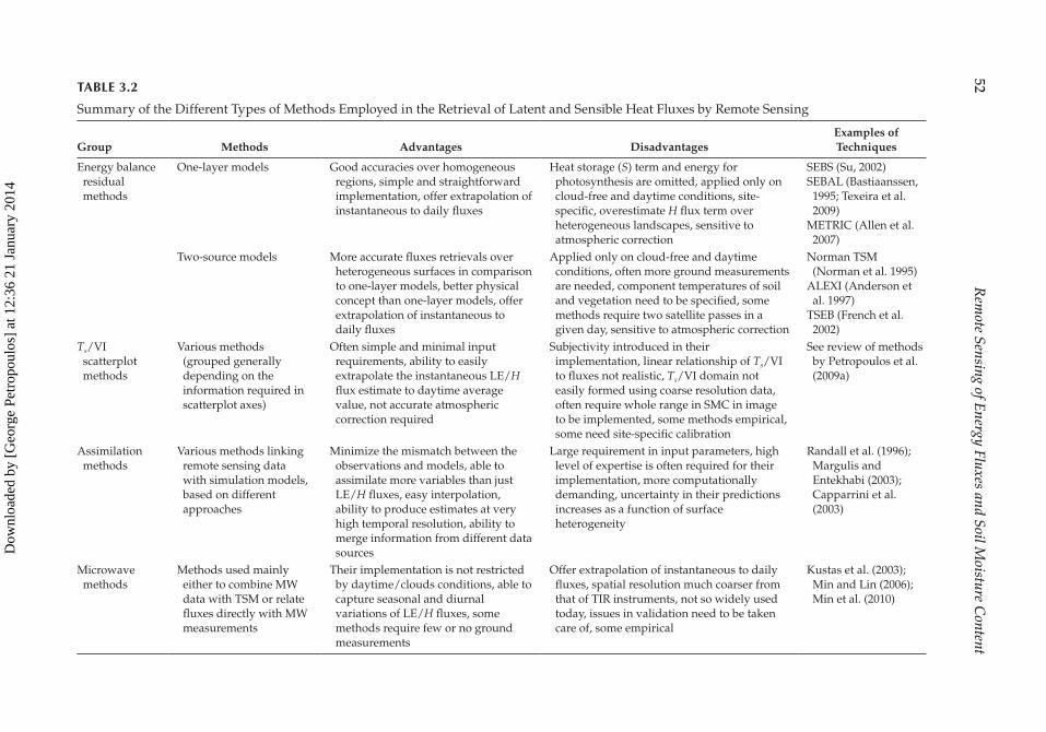
An overview of the remote sensing–based estimation of LE and H turbulent fluxes is provided next, following largely the classification of the techniques proposed by other investigators (e.g., Glenn et al. 2007; Gowda et al. 2008; Li et al. 2009b; Petropoulos et al. 2009a). A summary of the relative strengths and limitations of the techniques reviewed is also made available in Table 3.2.
3.2.1 Residual Methods of Surface Energy Balance
Development of residual methods is traced back to the early 1970s (Sone and Horton 1974; Verma et al. 1976). The vast majority of these approaches are fundamentally based on the principles of energy conservation. In those techniques, generally land surface character-istics such as albedo, leaf area index (LAI), vegetation indices (VIs), surface roughness, surface emissivity, and surface temperature (Ts) are derived from satellite observations. Those parameters are subsequently combined with ground observations to produce spa-tially distributed maps of fluxes of net radiation (Rn), soil heat (G), and H fluxes. Then, the LE flux is computed as a residual of the energy balance equation.
In mathematical terms, for a typical vegetated land surface the energy balance equation is expressed as
Rn − G − S − H − LE = 0 (3.1)
where Rn is the net radiation (net short and net longwave), G is the soil heat flux, and S is the rate of heat storage in the plant canopy due to photosynthesis (W m–2). The quantity (Rn – G) is commonly called the “available energy” (e.g., Diak et al. 2004).
TABLE 3.1
Examples of Spaceborne Sensors Currently in Orbit Providing Observations Appropriate to Derive Surface Heat Fluxes
Sensor Manufacturer Platform Spatial ResolutionSpectral
ResolutionTemporal
Resolution
ASTER NASA/ERSDAC
Terra VNIR: 15 mSWIR: 30 mTIR: 90 m
VNIR: 4SWIR: 6TIR: 5
16 days
Landsat TM/ETM+
NASA/U.S. Department of Defense
Landsat VNIR: 30 mSWIR: 30 m
TIR: 120 m (TM)/60 m (ETM+)
VNIR: 4SWIR: 2TIR: 1
16 days
MODIS NASA Terra and Aqua
VNIR: 250 m/500 mSWIR: 500 m
TIR: 1 km
VNIR: 18SWIR: 2TIR: 16
2 daytime/2 nighttime
AVHRR/3 NASA NOAA VNIR: 1.1 kmSWIR: 1.1 kmTIR: 1.1 km
VNIR: 2SWIR: 1TIR: 2/3
2 daytime/2 nighttime
AATSR ESA ENVISAT VNIR: 1 kmSWIR: 1 kmTIR: 1 km
VNIR: 3SWIR: 1TIR: 3
2 daytime/2 nighttime
SEVIRI EUMETSAT/ESA
Meteosat-2 VNIR: 1.1 and 3.0 km SWIR: 3 km
TIR: 3 km
VNIR: 4TIR: 8
96 scenesper day
(every 15’)
Dow
nloa
ded
by [
Geo
rge
Petr
opou
los]
at 1
2:36
21
Janu
ary
2014
52R
emote Sensing of Energy Fluxes and Soil M
oisture Content
TABLE 3.2
Summary of the Different Types of Methods Employed in the Retrieval of Latent and Sensible Heat Fluxes by Remote Sensing
Group Methods Advantages DisadvantagesExamples of Techniques
Energy balance residual methods
One-layer models Good accuracies over homogeneous regions, simple and straightforward implementation, offer extrapolation of instantaneous to daily fluxes
Heat storage (S) term and energy for photosynthesis are omitted, applied only on cloud-free and daytime conditions, site-specific, overestimate H flux term over heterogeneous landscapes, sensitive to atmospheric correction
SEBS (Su, 2002)SEBAL (Bastiaanssen, 1995; Texeira et al. 2009)
METRIC (Allen et al. 2007)
Two-source models More accurate fluxes retrievals over heterogeneous surfaces in comparison to one-layer models, better physical concept than one-layer models, offer extrapolation of instantaneous to daily fluxes
Applied only on cloud-free and daytime conditions, often more ground measurements are needed, component temperatures of soil and vegetation need to be specified, some methods require two satellite passes in a given day, sensitive to atmospheric correction
Norman TSM (Norman et al. 1995)
ALEXI (Anderson et al. 1997)
TSEB (French et al. 2002)
Ts/VI scatterplot methods
Various methods (grouped generally depending on the information required in scatterplot axes)
Often simple and minimal input requirements, ability to easily extrapolate the instantaneous LE/H flux estimate to daytime average value, not accurate atmospheric correction required
Subjectivity introduced in their implementation, linear relationship of Ts/VI to fluxes not realistic, Ts/VI domain not easily formed using coarse resolution data, often require whole range in SMC in image to be implemented, some methods empirical, some need site-specific calibration
See review of methods by Petropoulos et al. (2009a)
Assimilation methods
Various methods linking remote sensing data with simulation models, based on different approaches
Minimize the mismatch between the observations and models, able to assimilate more variables than just LE/H fluxes, easy interpolation, ability to produce estimates at very high temporal resolution, ability to merge information from different data sources
Large requirement in input parameters, high level of expertise is often required for their implementation, more computationally demanding, uncertainty in their predictions increases as a function of surface heterogeneity
Randall et al. (1996); Margulis and Entekhabi (2003); Capparrini et al. (2003)
Microwave methods
Methods used mainly either to combine MW data with TSM or relate fluxes directly with MW measurements
Their implementation is not restricted by daytime/clouds conditions, able to capture seasonal and diurnal variations of LE/H fluxes, some methods require few or no ground measurements
Offer extrapolation of instantaneous to daily fluxes, spatial resolution much coarser from that of TIR instruments, not so widely used today, issues in validation need to be taken care of, some empirical
Kustas et al. (2003); Min and Lin (2006); Min et al. (2010)
Dow
nloa
ded
by [
Geo
rge
Petr
opou
los]
at 1
2:36
21
Janu
ary
2014
53Remote Sensing of Surface Turbulent Energy Fluxes
The S term in Equation 3.1 generally is less than a few percent of Rn (Meyers and Hollinger 2004). It is also a parameter that quantitatively is not easy to be measured even by ground instrumentation (Wilson et al. 2001). As a result, in most remote sensing energy balance–based approaches for the computation of LE flux, this term is generally omitted. Nevertheless, it should be noted that in the case of vegetation types with a significant can-opy amount (e.g., as forests), S can become high particularly so over instantaneous periods (Meyers and Hollinger 2004; Sanchez et al. 2008).
The Rn term represents the total heat energy partitioned into G, H, and LE fluxes. Rn is generally modeled as the sum of the incoming and outgoing radiation components of the shortwave and longwave portions. Previous research has demonstrated that Rn can be calculated from well-established approaches based on primarily remotely sensed data. Generally, comparisons between modeled and ground-based measurements of Rn have shown an uncertainty in the estimation of Rn by remote sensing in the range of 5%–10% in comparison to ground observations (e.g., Sanchez et al. 2008; Yang et al. 2010). An over-view of the EO-based methods employed in deriving all the components of Rn including relevant operational products currently available can be found in Chapter 5.
The G flux is defined as the heat energy responsible for changing the temperature of the substrate soil volume. When Equation 3.1 above is evaluated over a 24-h time period, G flux is commonly assumed to be negligible. However, when Equation 3.1 is applied on an instan-taneous basis as is the case when satellite observations are used, the assumption of neglect-ing G is not valid. Hence, in such cases, evaluation of the instantaneous LE flux as a residual term from the energy balance equation makes indispensable the computation of the G flux component. Remote sensing approaches for the G flux estimation have been largely based on assumptions developed around relationships between the ratio of G/Rn and satellite-derived vegetation indices (VIs). Comparison studies specifically of G flux predicted by such simpli-fied techniques versus in situ observations have shown an uncertainty of 20%–30% in the estimation of G flux alone (Kustas and Norman 1996; Li et al. 2009b; Ma et al. 2011).
Yet, remote sensing–based estimation of H flux is the most difficult and also challeng-ing to be derived. The main difficulties relate essentially to the uncertainty introduced in the estimation of the aerodynamic and surface resistances. This is because those vary considerably spatially, particularly as a function of surface heterogeneity (e.g., Schmugge et al. 2002; Verstraeten et al. 2008). Thus, as H flux essentially introduces the largest uncer-tainty in the LE flux estimation, the methods in which LE flux is computed as a residual from the energy balance equation differ essentially on the way the H flux term is mod-eled. Generally, H flux prediction accuracy has been found to be largely dependent on the complexity by which the soil and vegetation components are modeled (Norman et al. 2003; Courault et al. 2005; Li et al. 2009b). Thus the remote sensing–based methods employed are generally divided into two broad categories, depending on whether or not the land surface is modeled as a single land surface or is separated into bare soil and vegetation layers, so-called “one-layer” and “two-source (or dual layer)” models, respectively.
The remainder of this section provides an overview of the use of the most widely used one- and two-layer modeling schemes by the remote sensing community. A detailed account to some of these modeling schemes including examples from case studies is pro-vided in Part II of the volume.
3.2.1.1 One-Layer Models
In the case of one-layer approaches, the most commonly applied method to estimate region-ally H flux from EO data is by the use of remotely derived radiometric surface temperature
Dow
nloa
ded
by [
Geo
rge
Petr
opou
los]
at 1
2:36
21
Janu
ary
2014
54 Remote Sensing of Energy Fluxes and Soil Moisture Content
(Ts). The physical concept for the use of temperature measurements in the estimation of H flux originates from Monteith and Szeicz (1962) and Monteith (1963) and is based in the following expression:
H C
T TRp
o A
A
= −ρ (3.2)
where ρ is the air density (kg m–3), Cp is the specific heat of air at constant pressure (J kg–1 K–1) [the component ρCp is called the volumetric heat capacity (J m–3 °C–1)], T0 is the aerodynamic temperature (°C, this parameter relates to the efficiency of heat exchange between the land surface and overlying atmosphere), TA is the air temperature (°C) at a reference height, and RA is the aerodynamic resistance between canopy height and the ambient environment above the canopy (s m–1).
Equation 3.2 is a one-layer bulk transfer equation and is based on the assumption that the radiometric surface temperature (TR(θ)) measured by a thermal radiometer is identical or very close to the aerodynamic temperature (To) (e.g., Asrar 1989; Bastiaanssen 2000). Yet, although the surface brightness temperature is approximately the same as aerodynamic temperature over non-vegetated surfaces, it is not the same over most naturally vegetated surfaces. Estimation errors in the H flux even of the order of 100 W m–2 have been reported when (TR(θ)) is simply used to replace To and if atmospheric effects and surface emissivity are not properly considered (Chavez and Neale 2003; Gowda et al. 2008). Thus, to account for this difference, in the one-layer modeling schemes an extra resistance (REX) is added to RA in Equation 3.2, which takes the following form:
H C
T TR RpR A
A EX
= −+
ρ θ( ) (3.3)
where REX is the so-called excess resistance, which accounts for the non-equivalence of To and TR(θ).
RA is usually estimated using local data on wind speed, stability conditions, and rough-ness length, even though area averaging of roughness lengths is considered to be highly nonlinear (Hasager and Jensen 1999). A number of one-layer models have been developed so far based on the above concept. Some of the most widely used ones by the remote sens-ing community are reviewed below.
3.2.1.1.1 Surface Energy Balance System
Surface Energy Balance System (SEBS) is a one-layer model developed by Su (2002) for the estimation of surface energy balance parameters including the LE and H fluxes. Briefly, SEBS consists of three components: (1) a set of algorithms used for the estima-tion of different components of energy balance and relevant land surface parameters; (2) an extended model to establish the roughness length for heat transfer (Su 2002); and (3) a formulation to extrapolate the instantaneous flux estimates to daytime aver-age and daily totals based on the energy balance at limiting wet and dry cases. SEBS generally requires input parameters derived by both remote sensing (e.g., albedo, emis-sivity, temperature, vegetation cover, and LAI) and ground observations (air pressure, humidity, and wind speed at a reference height). A more detailed description of SEBS with results from its implementation in different case studies is furnished in Chapter 7,
Dow
nloa
ded
by [
Geo
rge
Petr
opou
los]
at 1
2:36
21
Janu
ary
2014
55Remote Sensing of Surface Turbulent Energy Fluxes
whereas reference to this model from an operational perspective is made as well in Chapter 10.
SEBS ability to compute LE and H fluxes has been generally evaluated over a range of land cover types using different types of EO data. For example, Su et al. (2005) evalu-ated SEBS with Landsat ETM+ imagery over an agricultural area in Iowa, United States, using ground observations from a SMACEX field experiment. Authors reported the SEBS-derived LE fluxes to be ~90% to the corresponding ground measurements of LE acquired over different crop types. In another study, McCabe and Wood (2006) showed the LE flux retrievals from Landsat exhibiting closer agreement to ground measurements (RMSD = 61.94 W m–2) in comparison to when SEBS was combined with ASTER-derived data (RMSD = 82.04 W m–2). Yang et al. (2010) evaluated SEBS using coarser resolution MODIS data acquired over a mainly cropland area in north China. Comparisons of the LE and H fluxes predicted by SEBS versus concurrent eddy covariance in situ measurements showed a sig-nificant underestimation of the H fluxes by SEBS and an overestimation of the LE fluxes with biases of –28 and 103 W m–2, respectively. Ma et al. (2011) using ASTER data acquired over a region in China evaluated SEBS ability to predict different components of the energy balance. Energy flux components estimated from SEBS were predicted in their study with acceptable accuracy over partially vegetated areas such as their test region.
Some of SEBS advantages include the following: (1) the uncertainty from the surface temperature or meteorological variable estimation in SEBS can be limited with consider-ation of the energy balance at the limiting cases; (2) formulation of the roughness height for heat transfer in SEBS is not based on using fixed values; and (3) a priori knowledge of the actual turbulent heat fluxes is not required by the model. However, SEBS opera-tion is possible only on clear sky days. Yet, perhaps the main limitation of SEBS is that it requires aerodynamic roughness height to be estimated, a parameter of which estimation by remote sensing actually remains a challenge until today (Gowda et al. 2008).
3.2.1.1.2 Surface Energy Balance Algorithm for Land (SEBAL)
Surface energy balance algorithm for land (SEBAL) is exploiting both empirical relation-ships and physical parameterizations for computing the energy partitioning at the regional scale based primarily on EO data and a small number of ground observations. A full description of the SEBAL can be found in Bastiaanssen (1995) and Bastiaanssen et al. (1998). Briefly, key remote sensing input parameters to the model include the incoming radiation, Ts, Normalised Difference Vegetation Index (NDVI, Rouse et al. 1973), and albedo maps, whereas different semi empirical relationships are used for estimating variables such as emissivity and roughness length. First, the Rn and G fluxes are computed based on a series of parameters (e.g., surface temperature Ts, reflectance-derived albedo values, VIs, Leaf Area Index (LAI), and surface emissivity). H flux is subsequently estimated from a bulk aerodynamic resistance formulation and the temperature difference between the land sur-face and air computed from extreme (i.e., wet and dry) image pixels. Those are used to develop a linear relationship between temperature difference and surface temperature. Then, LE flux is solved as a residual from the energy balance equation. Chapter 6 pres-ents the workings of SEBAL implementation in more detail, providing results from case studies.
SEBAL ability to provide regional estimates of the different components of the energy balance equation has been extensively examined by many investigators using different types of EO data. For example, Bastiaanssen et al. (2005) evaluated SEBAL over different climatic conditions and spatial scales. An accuracy of 85% was reported by the authors in the estimation of LE fluxes at field scale, of 95% at seasonal scale, and of 96% at annual
Dow
nloa
ded
by [
Geo
rge
Petr
opou
los]
at 1
2:36
21
Janu
ary
2014
56 Remote Sensing of Energy Fluxes and Soil Moisture Content
scale. Bashir et al. (2008) using both Landsat ETM+ and MODIS image data acquired over a region in Sudan showed a mean absolute error in LE fluxes of approximately 0.9 mm day–1 for MODIS and of 0.9 mm day–1 for the Landsat images. Kongo et al. (2011) examined the combined use of SEBAL with MODIS imagery for deriving spatially distributed LE fluxes for a region in Africa analyzing in total 28 MODIS images. LE fluxes predicted by SEBAL showed a difference ranging from –14% to +26% in comparison to corresponding measurements derived from a large scintillometer. Recently, Sun et al. (2011) evaluated SEBAL using Landsat ETM+ data acquired over a wetland area in China. Authors reported an overestimation of the predicted daily LE estimates on the order of 10% in comparison to ground measurements from evaporation pans.
A key advantage of SEBAL is that the LE and H fluxes derived from this technique are not sensitive to accurate retrievals of Ts. This is because SEBAL accommodates an auto-matic internal calibration, which can be done separately for each image analyzed. Also, similar to SEBS, SEBAL implementation is based largely on EO-based inputs and a small number only of ground observations, which potentially make its implementation easy and cost-effective. Yet, it is dependent on the selection of representative pixels in an image for dry and wet conditions, which might include some degree of user subjectivity. Also, as underlined by Li et al. (2009b), SEBAL application over nonflat terrain sites requires mak-ing adjustments to certain input variables of the model (e.g., Ts), as otherwise prediction of the H and LE fluxes can be dramatically affected. Last but not least, SEBAL also requires cloud-free conditions and heterogeneity in moisture conditions to be implemented.
3.2.1.1.3 METRIC
METRIC (Allen et al. 2007) is essentially based on the SEBAL with the main difference being in the way of determining the wet and dry pixels. In particular, in contrast to SEBAL, METRIC does not make assumptions of zero H flux, neither that H = Rn – G at the wet image pixel; instead of that, a soil water budget is applied for the hot pixel to verify that LE flux is indeed zero. What is more, in METRIC the extreme pixels are selected in an agricultural setting in which cold pixels should have biophysical characteristics similar to the reference crop (alfalfa). Besides, another difference in comparison to SEBAL is that in METRIC the alfalfa reference evapotranspiration fraction (ETrF) mechanism is used to extrapolate instantaneous LE flux to daily flux rates. ETrF is defined as the ratio of the remotely sensed instantaneous LE flux (LE) to the reference LE flux (ETr, e.g., mm h–1), where the latter is derived at the time of the satellite overpass from ground data.
A number of experiments have been conducted attempting to appraise the use of METRIC for predicting the LE and H fluxes. Allen et al. (2007) evaluated METRIC in two agricultural areas in the Idaho area, United States, using in situ estimates from lysimeters and reported differences in LE ranging between 1% and 4%. Gowda et al. (2008) applied METRIC with Landsat TM acquired over an agricultural area located in Texas High Plains, United States. Comparisons of the daily LE fluxes predicted by the model versus predic-tions from a soil moisture budget showed a low error for the case of well-irrigated and high biomass corn vegetation [2.0 mm day–1 (17.1%) and 0.5 mm day–1 (6.0%) for each day]. Chavez et al. (2009) combined METRIC with Landsat TM for the Texas High Plains, United States. Authors reported a generally close agreement of METRIC-predicted daily LE fluxes in comparison to those derived from the lysimeters, with a mean bias error ±RMSD of 0.4 ± 0.7 mm day–1. Khan et al. (2010) compared LE fluxes predicted from METRIC using MODIS data acquired over several Ameriflux sites versus eddy covariance in situ reference measurements. A mean bias from the ground observations lower than 15% and a seasonal bias lower than 8% in the daily LE fluxes agreement was reported.
Dow
nloa
ded
by [
Geo
rge
Petr
opou
los]
at 1
2:36
21
Janu
ary
2014
57Remote Sensing of Surface Turbulent Energy Fluxes
Generally, METRIC is largely characterized by similar types of advantages and dis-advantages as the other one-layer models reviewed previously, specifically those of the SEBAL model. However, in comparison to SEBAL, various studies have indicated that METRIC appears to have an advantage over SEBAL in providing more accurate estimates of energy fluxes under advective conditions (e.g., Chavez et al. 2009).
3.2.1.2 Two-Source Models
Essentially, the development of the early two-source modeling (TSM) schemes can be traced back to the end of the 1980s. Shuttleworth and Wallace (1985) and Shuttleworth and Gurney (1990) were among the first to introduce the idea. Generally, in comparison to the one-layer models, in TSM schemes energy fluxes are partitioned between the soil and veg-etation allowing the estimation of the LE and H fluxes over incomplete canopies. A num-ber of TSMs have been proposed over the years. A review of some of the most widely used ones is provided in the remainder of this section, underlying their comparative advantages and disadvantages in respect to their practical implementation.
3.2.1.2.1 Norman et al. (1995) Model
A significant contribution to the TSM techniques development was made by Norman et al. (1995). Briefly, their TSM was based on the assumption that the contribution of the canopy and soil layers to H fluxes depends on the temperature differences between each layer and the atmosphere and on the coupling that is assumed to be between layers. Retrievals of the LE and H fluxes from the Normal et al. (1995) model have also been the subject of many stud-ies conducted in different regions. Norman et al. (1995) first evaluated their TSM using data from FIFE (Sellers et al. 1992) and MONSOON 90 (Kustas et al. 1991) field campaigns. Authors reported Root Mean Square Difference (RMSD) between the model predictions and corre-sponding in situ measurements between 35 and 60 W m–2 for G, H, and LE fluxes, respectively. French et al. (2000) evaluated independently the Norman et al. (1995) model using airborne remote sensing data from the Thermal Infrared Multispectral Scanner (TIMS) acquired in the SMACEX and SMEX02 field experiments in the United States. Their results showed H fluxes predictions close to in situ eddy covariance with average differences of 43 W m–2.
Gonzalez-Dugo et al. (2009) using Landsat TM imagery examined the model of Norman et al. (1995) and a one-layer model in terms of their ability to estimate the surface fluxes. The Norman et al. (1995) model returned slightly more accurate predictions of the H and LE fluxes, in comparison to the one-layer model, with an RMSD lower than 31 W m–2 in the estimation of the H fluxes. Li et al. (2008) evaluated the effect of pixel resolution to the energy fluxes computed from the model of Norman et al. (1995) using Landsat TM images and in situ data collected in 2004 during the Soil Moisture Field Experiment (SMEX) con-ducted in Arizona, United States. In their study, the Norman et al. (1995) TSM was imple-mented at three spatial resolutions, namely, 30, 120, and 960 m. A generally satisfactory agreement was found between predicted and in situ measurements in the heat fluxes for the case of the 30 and 120 m spatial resolution, with RMSDs between 20 and 35 W m−2 and a mean RMSD of 33 W m–2. However, for the comparisons at 960 m, agreement between the compared LE fluxes was comparatively lower, with a mean RMSD of 40 W m–2. The latter was attributed by the authors to the inferior representation of the land surface heterogene-ity, which was not possible to be depicted at this coarse spatial resolution.
In contrast to the one-layer models reviewed in the previous section, the Norman et al. (1995) TSM has the advantage that it contains the difference between radiometric tem-perature and aerodynamic temperature. The latter overcomes the problem of an empirical
Dow
nloa
ded
by [
Geo
rge
Petr
opou
los]
at 1
2:36
21
Janu
ary
2014
58 Remote Sensing of Energy Fluxes and Soil Moisture Content
resistance depending on the radiometer view angle. In addition, the model offers the advantage that can account for variation in surface resistances due to variation in vegeta-tion cover and surface roughness, without requiring redefinition of “excess” resistance without any additional ground observations.
3.2.1.2.2 ALEXI/DISALEXI Model
Another TSM scheme was developed by Anderson et al. (1997). Their model was initially named Two-Source Time Integrated Model (TSTIM) and was later renamed by Mecikalski et al. (1999) as Atmosphere-Land Exchange Inverse (ALEXI). In comparison to the Norman et al. (1995) TSM, ALEXI’s main difference is that it includes a scheme where the growth of the atmospheric boundary layer (ABL) is coupled to the temporal changes in surface radiometric temperature from the Geosynchronous Operational Environmental Satellite (GOES). Detailed description of the model can be found in the work of Anderson et al. (1997) and also in Chapter 8, which also presents case studies of practical applications of the model outputs in monitoring drought and crop condition.
Validation of ALEXI by Anderson et al. (1997) and later by Mecikalski et al. (1999) with ground data from the FIFE (Sellers et al. 1992) and MONSOON’90 (Kustas et al. 1991) field campaigns confirmed the model’s ability to estimate LE and H fluxes with uncertainty at least comparable to other modeling schemes. Later, Kustas et al. (2003) and Norman et al. (2003) developed a scheme that they called the Disaggregated Atmosphere Land Exchange Inverse model (DisALEXI). That allowed deriving spatially distributed estimates of the energy fluxes by combining low- and high-resolution satellite observations without the need of local observations. Authors demonstrated the use of DisALEXI from Southern Great Plains, United States. Their comparisons showed an agreement between the pre-dicted surface fluxes and corresponding ground-based measurements within 10%–12%. An overview of the ALEXI/DISALEXI model including results from the model use in vari-ous locations of the world was provided recently by Anderson et al. (2010).
All in all, a key advantage of ALEXI in comparison to other TSMs including the Norman et al. (1999) model reviewed earlier is that it allows taking into consideration the temporal changes of brightness temperatures and relates the rise in air temperature above the can-opy and the growth of the Atmosphere Boundary Layer (ABL) to the time-integrated fluxes from the surface. This, as argued by the model developers, dramatically reduces the errors in the conversion to radiometric surface temperatures due to uncertainties associated to emissivity and atmospheric correction. Besides, ALEXI is able to take under consideration the viewing angle effects in the calculation of vegetation fraction. Also, in comparison to other one-layer and TSMs, ALEXI is able to offer a scheme for disaggregating the predicted fluxes at spatial resolutions of moderate and fine resolution thermal infrared imagery from polar-orbiting systems. The latter allows generating daily maps of surface heat fluxes at very high spatial resolution (Anderson et al. 2010).
3.2.1.2.3 TSEB Model
The Two-Source Energy Balance (TSEB) model developed by French et al. (2002) consisted essentially of a refinement of the original Norman et al. (1995) model that was conducted, where Ts was derived by employing the temperature emissivity separation (TES) algorithm (Gillespie et al. 1998) using the ASTER thermal bands. Thus TSEB was particularly suitable for computing LE fluxes from high spatial resolution multispectral data such as those from the ASTER sensor. French et al. (2002) compared surface heat fluxes by TSEB against corre-sponding in situ observations from the Bowen ratio. TSEB returned a nearly ideal estimate of LE fluxes in their study. However, significant discrepancies with respect to the ground
Dow
nloa
ded
by [
Geo
rge
Petr
opou
los]
at 1
2:36
21
Janu
ary
2014
59Remote Sensing of Surface Turbulent Energy Fluxes
measurements were reported in the remaining flux components, with the most significant one being the H flux overestimated by TSEB by 90 W m–2. Anderson et al. (2008) investi-gated the use of a canopy light use efficiency based model within TSEB, using as a case study the SGP97 field experiment data from the El Reno experimental site in the United States. Authors showed that this replacement resulted in a reduction in the predicted error in LE fluxes estimation by TSEB from 15% to 9% for LE flux and from 16% to 12% for all the other energy balance components combined. Sanchez et al. (2008) introduced a sim-plified version of TSEB, called the Simplified Two-Source Energy Balance (STSEB) model. Their model was aimed for use specifically with the dual-angle instrument ATSR. Authors evaluated STSEB for a test site in Maryland, United States, using input data acquired from ground instrumentation rather than remote sensing radiometers. An RMSD ranging from 15 to 50 W m–2 in the prediction of the Rn, G, LE, and H fluxes by their model was reported in comparisons performed versus eddy covariance ground measurements.
3.2.2 Methods Based on the Ts/VI Scatterplot
A different group of techniques employed for the estimation of hydrometeorological fluxes from remote sensing data has its basis on the relationships between a satellite-derived VI and surface temperature (Ts), when these are plotted in a scatterplot. An overview of the theoretical basis of these methods including the biophysical properties encapsulated on a Ts/VI scatterplot can be found in Petropoulos et al. (2009a).
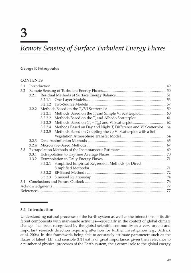
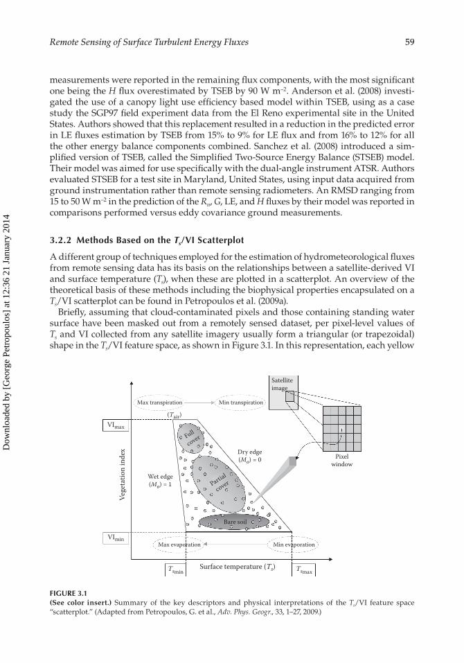
Briefly, assuming that cloud-contaminated pixels and those containing standing water surface have been masked out from a remotely sensed dataset, per pixel-level values of Ts and VI collected from any satellite imagery usually form a triangular (or trapezoidal) shape in the Ts/VI feature space, as shown in Figure 3.1. In this representation, each yellow
Max transpiration Min transpiration
Satelliteimage
Pixelwindow
Full
cover
Partial
cover
Surface temperature (Ts)
Vege
tatio
n in
dex Dry edge
(Mo) = 0
VImax
VImin
Tsmin Tsmax
Wet edge(Mo) = 1
(Tair)
Max evaporation Min evaporation
Bare soil
FIGURE 3.1(See color insert.) Summary of the key descriptors and physical interpretations of the Ts/VI feature space “scatterplot.” (Adapted from Petropoulos, G. et al., Adv. Phys. Geogr., 33, 1–27, 2009.)
Dow
nloa
ded
by [
Geo
rge
Petr
opou
los]
at 1
2:36
21
Janu
ary
2014
60 Remote Sensing of Energy Fluxes and Soil Moisture Content
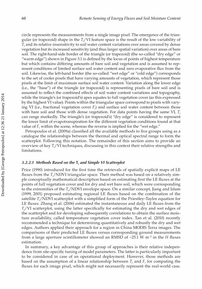
circle represents the measurements from a single image pixel. The emergence of the trian-gular (or trapezoid) shape in the Ts/VI feature space is the result of the low variability of Ts and its relative insensitivity to soil water content variations over areas covered by dense vegetation but its increased sensitivity (and thus larger spatial variation) over areas of bare soil. The right-hand-side border of the triangle (or trapezoid) (the so-called “dry edge” or “warm edge”) shown in Figure 3.1 is defined by the locus of points of highest temperature but which contains differing amounts of bare soil and vegetation and is assumed to rep-resent conditions of limited surface soil water content and zero evaporative flux from the soil. Likewise, the left-hand border (the so-called “wet edge” or “cold edge”) corresponds to the set of cooler pixels that have varying amounts of vegetation, which represent those pixels at the limit of maximum surface soil water content. Variation along the lower edge (i.e., the “base”) of the triangle (or trapezoid) is representing pixels of bare soil and is assumed to reflect the combined effects of soil water content variations and topography, while the triangle’s (or trapezoid’s) apex equates to full vegetation cover (as this expressed by the highest VI value). Points within the triangular space correspond to pixels with vary-ing VI (i.e., fractional vegetation cover Fr) and surface soil water content between those with bare soil and those with dense vegetation. For data points having the same VI, Ts can range markedly. The triangle’s (or trapezoid’s) “dry edge” is considered to represent the lower limit of evapotranspiration for the different vegetation conditions found at that value of Fr within the scene, whereas the reverse is implied for the “wet edge.”
Petropoulos et al. (2009a) classified all the available methods to five groups using as a catalogue the relationships between the thermal and optical spectral range to form the scatterplot. Following this notation. The remainder of this section aims to provide an overview of key Ts/VI techniques, discussing in this context their relative strengths and limitations.
3.2.2.1 Methods Based on the Ts and Simple VI Scatterplot
Price (1990) introduced for the first time the retrievals of spatially explicit maps of LE fluxes from the Ts/NDVI triangular space. Their method was based on a relatively sim-ple conceptually mathematical description based on estimating first the LE fluxes at the points of full vegetation cover and for dry and wet bare soil, which were corresponding to the extremities of the Ts/NDVI envelope space. On a similar concept, Jiang and Islam (1999, 2001) proposed estimating regional LE fluxes based on the combination of the satellite Ts/NDVI scatterplot with a simplified form of the Priestley–Taylor equation for LE fluxes. Zhang et al. (2006) estimated the instantaneous and daily LE fluxes from the Ts/VI scatterplot, using the latter specifically for estimating the dry and wet edges of the scatterplot and for developing subsequently correlations to obtain the surface mois-ture availability, called temperature vegetation cover index. Tan et al. (2010) recently recommended a technique for determining quantitatively and robustly the dry and wet edges. Authors applied their approach for a region in China MODIS Terra images. The comparisons of their predicted LE fluxes versus corresponding ground measurements from a large aperture scintillometer showed an RMSD of ~25.1 W m–2 in the H fluxes estimation.
In summary, a key advantage of this group of approaches is their relative indepen-dence from site-specific tuning of model parameters. The latter is particularly important to be considered in case of an operational deployment. However, those methods are based on the assumption of a linear relationship between Ts and Fr for computing the fluxes for each image pixel, which might not necessarily represent the real-world case.
Dow
nloa
ded
by [
Geo
rge
Petr
opou
los]
at 1
2:36
21
Janu
ary
2014
61Remote Sensing of Surface Turbulent Energy Fluxes
Last but not least, for a wider application of those methods, special attention should be paid to considering the impact of clouds, standing water, and sloping terrain, particu-larly on Ts estimation.
3.2.2.2 Methods Based on the Ts and Albedo Scatterplot
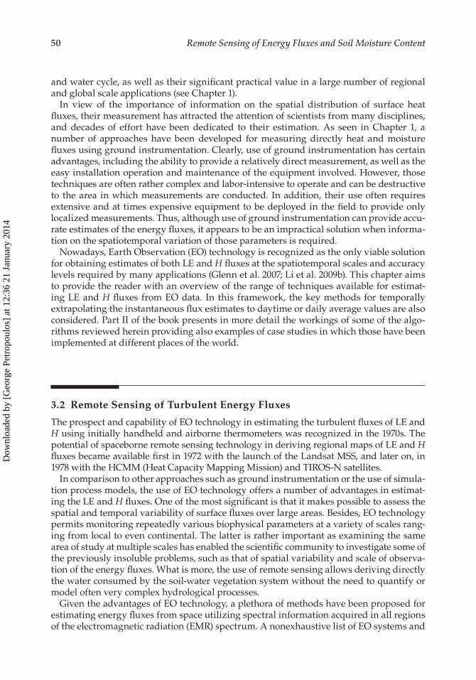
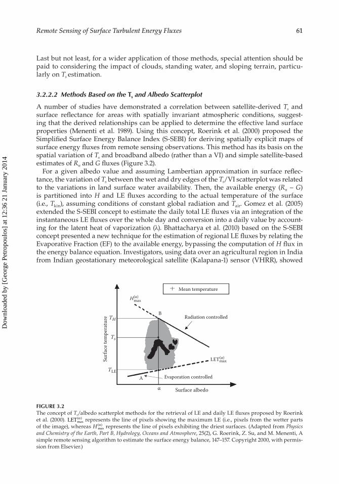
A number of studies have demonstrated a correlation between satellite-derived Ts and surface reflectance for areas with spatially invariant atmospheric conditions, suggest-ing that the derived relationships can be applied to determine the effective land surface properties (Menenti et al. 1989). Using this concept, Roerink et al. (2000) proposed the Simplified Surface Energy Balance Index (S-SEBI) for deriving spatially explicit maps of surface energy fluxes from remote sensing observations. This method has its basis on the spatial variation of Ts and broadband albedo (rather than a VI) and simple satellite-based estimates of Rn and G fluxes (Figure 3.2).
For a given albedo value and assuming Lambertian approximation in surface reflec-tance, the variation of Ts between the wet and dry edges of the Ts/VI scatterplot was related to the variations in land surface water availability. Then, the available energy (Rn – G) is partitioned into H and LE fluxes according to the actual temperature of the surface (i.e., Tkin), assuming conditions of constant global radiation and Tair. Gomez et al. (2005) extended the S-SEBI concept to estimate the daily total LE fluxes via an integration of the instantaneous LE fluxes over the whole day and conversion into a daily value by account-ing for the latent heat of vaporization (λ). Bhattacharya et al. (2010) based on the S-SEBI concept presented a new technique for the estimation of regional LE fluxes by relating the Evaporative Fraction (EF) to the available energy, bypassing the computation of H flux in the energy balance equation. Investigators, using data over an agricultural region in India from Indian geostationary meteorological satellite (Kalapana-1) sensor (VHRR), showed
Surface albedo
Evaporation controlled
Radiation controlled
Mean temperature
A
B
α
LET(α)
H(α)
Surfa
ce te
mpe
ratu
re TH
Ts
TLE
max
max
FIGURE 3.2The concept of Ts/albedo scatterplot methods for the retrieval of LE and daily LE fluxes proposed by Roerink et al. (2000). LETmax
( )α represents the line of pixels showing the maximum LE (i.e., pixels from the wetter parts of the image), whereas H max
( )α represents the line of pixels exhibiting the driest surfaces. (Adapted from Physics and Chemistry of the Earth, Part B, Hydrology, Oceans and Atmosphere, 25(2), G. Roerink, Z. Su, and M. Menenti, A simple remote sensing algorithm to estimate the surface energy balance, 147–157. Copyright 2000, with permis-sion from Elsevier.)
Dow
nloa
ded
by [
Geo
rge
Petr
opou
los]
at 1
2:36
21
Janu
ary
2014
62 Remote Sensing of Energy Fluxes and Soil Moisture Content
that predicted daily ET fluxes by their method were within the range of 25%–32% of the in situ observations. Various studies have evaluated S-SEBI in deriving spatially distrib-uted maps of energy fluxes at different environmental conditions (e.g., Roerink et al. 2000; Sobrino et al. 2007; Zahira et al. 2009). It generally appears that instantaneous and daily LE fluxes can be derived with accuracy of about 50 W m–2 and 1 mm day–1, respectively.
A key advantage of this group of approaches is their independence from additional meteorological data, provided that surface hydrological extremes are present in the image. What is more, in contrast to other Ts/VI methods reviewed thus far that attempt to deter-mine a fixed temperature for wet and dry conditions representative of the entire area of interest and/or for each land use class, this type of method assumes that the extreme tem-peratures for the wet and dry conditions vary with changing surface reflectance; the latter might appear a more realistic assumption. An important advantage of the Bhattacharya et al. (2010) technique, in particular, is that it can be implemented without the need of any ground observations. This is making potentially their method a very good choice for operational use. Also, their method avoids computation of H flux. Yet, generally speaking, between the key limitations of those approaches is their applicability on cloud-free days only and their requirement of identifying extreme points in the scatterplot domain. Also, the method proposed by Gomez et al. (2005) requires Ts measurements for both bare soil and full vegetation cover and the assumption of constant atmospheric conditions (mainly global radiation, wind speed, and Tair) over the entire studied region. Thus large prediction errors in LE flux can be returned when applied over areas of highly varying atmospheric conditions.
3.2.2.3 Methods Based on (Ts − Tair) and VI Scatterplot
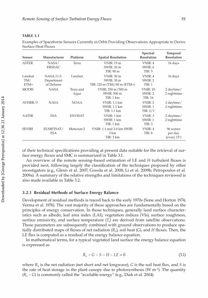
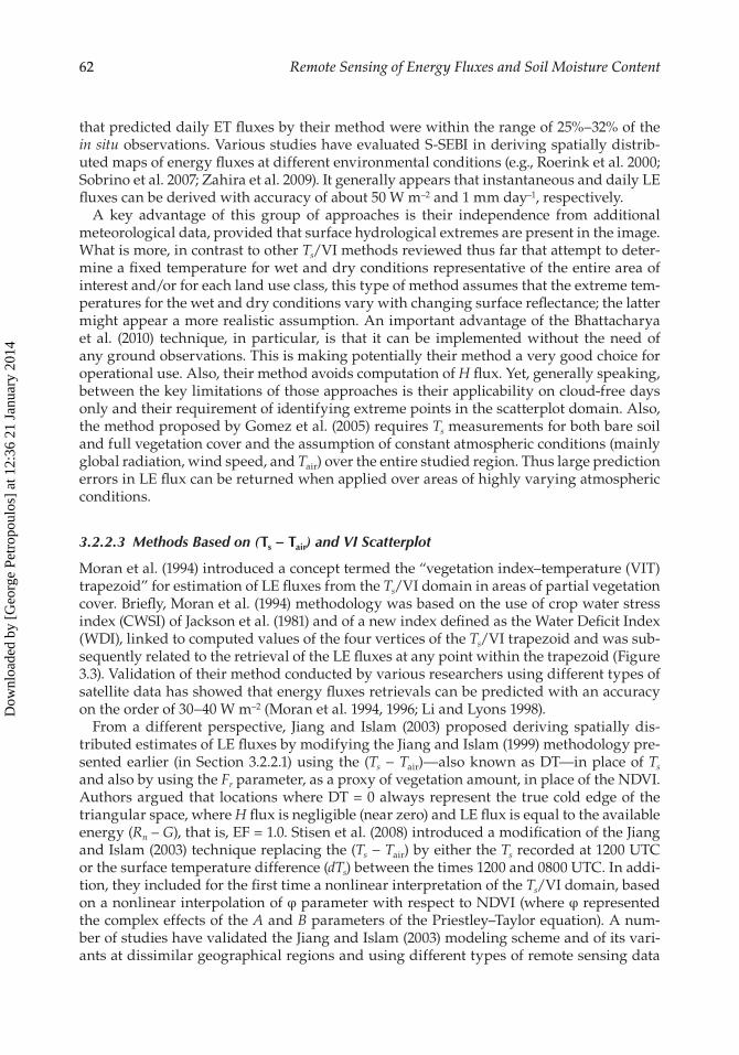
Moran et al. (1994) introduced a concept termed the “vegetation index–temperature (VIT) trapezoid” for estimation of LE fluxes from the Ts/VI domain in areas of partial vegetation cover. Briefly, Moran et al. (1994) methodology was based on the use of crop water stress index (CWSI) of Jackson et al. (1981) and of a new index defined as the Water Deficit Index (WDI), linked to computed values of the four vertices of the Ts/VI trapezoid and was sub-sequently related to the retrieval of the LE fluxes at any point within the trapezoid (Figure 3.3). Validation of their method conducted by various researchers using different types of satellite data has showed that energy fluxes retrievals can be predicted with an accuracy on the order of 30–40 W m–2 (Moran et al. 1994, 1996; Li and Lyons 1998).
From a different perspective, Jiang and Islam (2003) proposed deriving spatially dis-tributed estimates of LE fluxes by modifying the Jiang and Islam (1999) methodology pre-sented earlier (in Section 3.2.2.1) using the (Ts − Tair)—also known as DT—in place of Ts and also by using the Fr parameter, as a proxy of vegetation amount, in place of the NDVI. Authors argued that locations where DT = 0 always represent the true cold edge of the triangular space, where H flux is negligible (near zero) and LE flux is equal to the available energy (Rn – G), that is, EF = 1.0. Stisen et al. (2008) introduced a modification of the Jiang and Islam (2003) technique replacing the (Ts − Tair) by either the Ts recorded at 1200 UTC or the surface temperature difference (dTs) between the times 1200 and 0800 UTC. In addi-tion, they included for the first time a nonlinear interpretation of the Ts/VI domain, based on a nonlinear interpolation of φ parameter with respect to NDVI (where φ represented the complex effects of the A and B parameters of the Priestley–Taylor equation). A num-ber of studies have validated the Jiang and Islam (2003) modeling scheme and of its vari-ants at dissimilar geographical regions and using different types of remote sensing data
Dow
nloa
ded
by [
Geo
rge
Petr
opou
los]
at 1
2:36
21
Janu
ary
2014
63Remote Sensing of Surface Turbulent Energy Fluxes
(Jiang and Islam 2003; Venturini et al. 2004; Batra et al. 2006; Stisen et al. 2008; Shu et al. 2011). Such studies have shown that this group of methods are able to often provide esti-mates of instantaneous energy fluxes at an accuracy of about 50 W m–2 and daytime fluxes (expressed by the term evaporative fraction E which will be discussed later on) from 0.08 to 0.19, respectively.
Overall, a very important advantage of this group of methods is their independence from absolute accuracy of the Ts measures. This is because DT equal to zero always repre-sented the true cold edge of the triangle/trapezoidal domain where EF equals zero. Also, all methods were dependent on a very small number of in situ observations, for example, the Moran et al. (1996) method was dependent only on Rn, vapor pressure deficit, wind speed, and Tair. Clearly, the most important advantage of the latter approach in particular was the use of the WDI, which allowed a relatively straightforward computation of the instantaneous LE fluxes within the trapezoidal domain for both heterogeneous and homo-geneous surfaces, in contrast with the CWSI that was applicable only for homogeneous areas. Specifically the technique proposed by Stisen et al. (2008) has the advantage that included the utilization of the high temporal resolution geostationary MSG SEVIRI data, which allows the monitoring of the temperature diurnal variation. A further advantage of this is that it provides a nonlinear assumption of the triangular/trapezoid domain of (Fr, DT) feature space in solving for the energy fluxes, which might be a more realistic approxi-mation of reality. Yet, the Stisen et al. (2008) technique does not allow for the presence of water stress over full Fr where EF is zero along the observed dry edge.
1
0.8
0.6
0.4
0.2
0–10 0
3: Saturated bare soil
1: Well-watered vegetation
2: Water-stressed vegetation
4: Dry baresoil
10 20
A C
Ts – Ta (C)
Soil-
adju
sted
veg.
inde
x (S
AVI)
B
FIGURE 3.3Illustration of the principles of the trapezoidal method of Moran et al. (1994) for the estimation of the instan-taneous LE fluxes from the (Ts – Tair)/VI domain. Ts is the land surface temperature and Ta is the surface air temperature. According to the authors, having a measurement of (Ts – Ta) at any point C inside the trapezoid allows one to equate the ratio of actual to potential LE with the ratio of the distances CB and AB. (Adapted from Remote Sensing Environment, 49, M. S. Moran, T. R. Clarke, Y. Inoue, and A. Vidal, Estimating crop water deficit using the relation between surface-air temperature and spectral vegetation index, 246–263. Copyright 1994, with permission from Elsevier.)
Dow
nloa
ded
by [
Geo
rge
Petr
opou
los]
at 1
2:36
21
Janu
ary
2014
64 Remote Sensing of Energy Fluxes and Soil Moisture Content
3.2.2.4 Methods Based on Day and Night Ts Difference and VI Scatterplot
Briefly, implementation of this group of methods has been based on the existence of a strong relationship between the daytime and nighttime Ts and soil moisture and thermal inertia (van de Griend 1985; Jordan and Shih 2000). Tan (1998) and Chen et al. (2002) first proposed the idea of the LE fluxes retrieval from the difference between the day and night Ts versus the radiometric VI via a modeling scheme they called diurnal surface tempera-ture variation (DSTV). DSTV has been based on implementing firstly a simple linear mix-ture model on the DSTV/VI domain to determine the fractional contributions of the values for each pixel from vegetation, dry soil, and wet soil surfaces. Then, an index is computed termed “vegetation and moisture coefficient,” which for each image pixel was expressed as the sum of the weighted components from vegetation cover, dry soil, and wet soil. The latter is used to determine the actual LE flux, following the procedure detailed by Chen et al. (2002). Wang et al. (2006) proposed a variant of the Jiang and Islam (2003) method, in which the daytime Ts was replaced by the day – night Ts difference and NDVI (ΔTs – NDVI).
Validation studies on techniques belonging to this group of approaches have generally showed errors in the prediction of daily evapotranspiration between 2.8% and 23.9% and RMSDs varying from 3.08 to 5.74 mm day–1 (Tan 1998; Chen et al. 2002; Wang et al. 2006). Although their implementation appears to be dependent of only a very small number of ground measurements, those techniques have certain shortcomings. First of all, those methods are based on the assumption of three dominant land cover types in the mixture modeling scheme, which cannot always be found in a satellite scene. Also, the method requires for its implementation two satellite derived Ts observations, one acquired during daytime and one during nighttime conditions. Evidently, this condition cannot be satis-fied by all remote sensing sensors currently in orbit that are otherwise capable of being implemented by those methods.
3.2.2.5 Methods Based on Coupling the Ts / VI Scatterplot with a Soil Vegetation Atmosphere Transfer Model
An alternative approach for deriving spatially distributed maps of LE and H fluxes, termed the “triangle” method, is based on the coupling of the Ts/VI feature space with a land bio-sphere model, namely, a Soil Vegetation Atmosphere Transfer (SVAT) model. SVAT models are essentially vertical views of hydrological processes that consider the transport of water and energy just below the surface across the interface and within and through the vegeta-tion canopy. This type of method aims to combine the horizontal coverage and spectral resolution of EO data with the vertical coverage and fine temporal continuity of SVAT models. At present, the “triangle” has been implemented with the SimSphere model (see Petropoulos et al. 2009b for a review of the model use); yet, any other SVAT model with similar functionalities can be used.
Overviews of the triangle method implementation can be found in the works of Carlson (2007) and Petropoulos and Carlson (2011). Briefly, this approach is based on a quantitative interpretation of the Ts/Fr scatterplot using a one-dimensional SVAT model the latest ver-sion of which is called SimSphere (distributed from Aberystwtyh University, UK, http://www.aber.ac.uk/simsphere), with constraints imposed by the warm edge and the extreme values of the Ts/Fr scatterplot for bare soil and full vegetation, respectively. The SVAT model is first initialized using representative test site data. Then, at the time of the sensor overpass the model is iterated for all possible combinations of Fr and Mo and the simulated outputs of Ts and the surface energy fluxes are recorded at each iteration. As the next step, a
Dow
nloa
ded
by [
Geo
rge
Petr
opou
los]
at 1
2:36
21
Janu
ary
2014
65Remote Sensing of Surface Turbulent Energy Fluxes
third-order polynomial equation is derived linking the modeled soil surface moisture (Mo) to the values of Ts and Fr, along with similar equations linking each of the LE and H fluxes to Mo and Fr. Although these equations are empirically derived, they are based on physical representations of the biophysical processes operating within the SVAT model simulation. Thus the technique can be used to provide estimates of Mo simultaneous to the retrievals of the surface heat fluxes.
Gillies et al. (1997) extended the method by proposing and the computation of the ratios of LE or H to Rn (LE/Rn or H/Rn) inside the triangle domain, along with the instantaneous energy fluxes and Mo derived at the time of satellite overpass. Brunsell and Gillies (2003) using the SVAT model within the “triangle” demonstrated a procedure to interpolate the satellite-derived temperatures at different times from that of the satellite overpass time. This allowed the authors to perform comparisons of the energy fluxes acquired at different overpass times. Petropoulos et al. (2009b, 2010, 2013) performed detailed sensitivity analysis to SimSphere, providing for the first time a detailed insight into its architecture and discuss-ing important implications of the model use within the “triangle” approach. A number of studies have evaluated the ability of this group of methods in deriving spatially distributed estimates of energy fluxes and Mo. It appears that the technique can predict instantaneous LE and H fluxes with a standard error in the order of ±10% and ±30%, respectively, and the daytime fluxes with an RMSD of around 0.15. Also, Mo prediction error can be about 16% (Gillies et al. 1997; Brunsell and Gillies 2003; Petropoulos and Carlson 2011).
In comparison to other Ts/VI techniques reviewed so far, the triangle group of methods has some noticeable advantages. First of all, contrary to all other Ts/VI techniques (except the recent study by Stisen et al. 2008), the “triangle” provides a nonlinear interpretation of the Ts/VI space and thus a solution for the computation of the spatially distributed estimates of the turbulent fluxes and Mo, which, in general, seems to be a more realistic assumption. Furthermore, the technique offers the potential of deriving additional param-eters, namely, the soil surface moisture and the daytime average LE and H fluxes via a relatively simple and straightforward way. Furthermore, the triangle puts forward the prospect to construct similar Ts/VI triangles on successive days with a virtually identical configuration of isopleths over the entire Ts/VI space, allowing to monitor land surface processes that can be linked to other phenomena (such as urbanization; e.g., Owen et al. 1998; Arthur-Hartanft et al. 2003). Last but not least, it offers the possibility to extrapolate the instantaneous estimates of the energy fluxes from one time of day to another as was recently demonstrated by Brunsell and Gillies (2003). Yet, potential downsides related to this method of implementation include the requirement of a large number of input param-eters in the SVAT model initialization and user expertise and familiarity that might be required with such type of model operation.
3.2.3 Data Assimilation Methods
Another approach in the regional estimation of surface heat fluxes includes the combined use of information derived from remote sensing with deterministic land surface process models, in some cases SVAT models. Models have some very important advantages, which justify their development and continuous use to contemporary modeling schemes together with EO data. Those are able to often provide access to a detailed description of soil and vegetation canopy processes and not only to a limited number of final variables such as evapotranspiration, soil moisture, or net primary production. Another important advan-tage is that their time resolution, which usually is less than 1 h, is in good agreement with the dynamic of atmospheric and surface processes. Because of their fine vertical coverage
Dow
nloa
ded
by [
Geo
rge
Petr
opou
los]
at 1
2:36
21
Janu
ary
2014
66 Remote Sensing of Energy Fluxes and Soil Moisture Content
and fine temporal continuity, land surface models have become attractive for applications combined with EO data, acquired instantaneously (Olioso 1992). This has led to a number of studies attempting to combine those models with EO data for obtaining spatially distrib-uted parameters characterizing land surface interaction processes, including surface heat fluxes. Overviews of assimilation approaches in remote sensing can be found for example in Kalma et al. (2008) and Li et al. (2009b). Generally, two types of approaches can be distin-guished: (1) the so-called forcing methods and (2) the assimilation methods.
Forcing methods are based on forcing the model input with the remote sensing mea-surement. Briefly, those methods consist of setting some of the input quantities in the model at values estimated from remote sensing measurements. Models’ parameterization usually requires an extensive amount of parameters, including information on vegeta-tion structure (e.g., LAI and height), optical properties of soil and vegetation, physiological properties of vegetation (e.g., stomatal conductance description, water transfer from soil to plants), thermal and hydraulic properties of the soil, and atmospheric conditions (e.g., air temperature and humidity, wind speed, incident radiation). Some of these parameters are derived from remote sensing. Various relevant studies have shown that the most adequate variables to be estimated from remote sensing are vegetation fraction (Fr), LAI, albedo, and emissivity (Courault et al. 2005). For example, the multilayer canopy–surface–layer terrestrial biosphere–atmosphere model Advanced Canopy–Atmosphere–Soil Algorithm (ACASA; Pyles et al. 2000) is an example of a forcing type of model developed to calculate face energy, mass, and momentum exchanges, as well as the microclimatic conditions, trace gas exchanges, and associated turbulence statistics, over vegetated regimes.
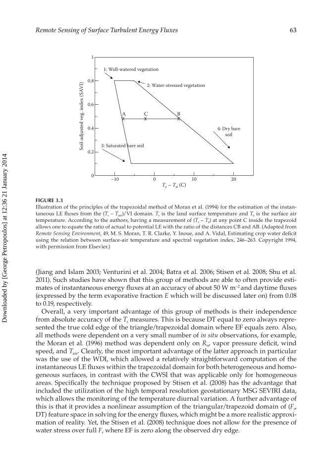
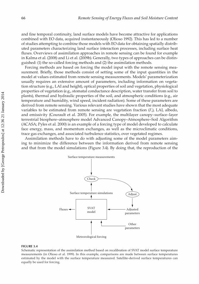
Assimilation methods have to do with adjusting some of the model parameters aim-ing to minimize the difference between the information derived from remote sensing and that from the model simulations (Figure 3.4). By doing that, the reproduction of the
Check
Adjust
Adjustedparameters
Otherparameters
SVATmodel
Fluxes
Meteorological forcing
Surface temperature simulations
Surface temperature measurements
FIGURE 3.4Schematic representation of the assimilation method based on recalibration of SVAT model surface temperature measurements (in Olioso et al. 1999). In this example, comparisons are made between surface temperatures estimated by the model with the surface temperature measured. Satellite-derived surface temperatures can equally be used for forcing.
Dow
nloa
ded
by [
Geo
rge
Petr
opou
los]
at 1
2:36
21
Janu
ary
2014
67Remote Sensing of Surface Turbulent Energy Fluxes
diurnal courses of canopy fluxes from instantaneous measurements is then possible (e.g., Soer 1980; Ottle and Vidal-Madjar 1994). Assimilation methods are generally divided into two subcategories, namely, (1) the sequential methods (e.g., Ensemble Kalman Filter and optimal interpolation) (Caparrini et al. 2003; Crow and Kustas 2005; Margulis et al. 2005), in which the course of state variables in the model is corrected at each time remote sens-ing data are available; and (2) the variational methods (e.g., four-dimensional variational assimilation, e.g., Margulis and Entekhabi 2003), where re-initialization or change of unknown parameters in the model is performed using data sets acquired over temporal windows of several days/weeks. In sequential assimilation, each individual observation influences the estimated state of the flow only at later times and not at previous times, whereas variational assimilation aims to adjust the model solution globally to all the observations available over the assimilation period (Talagrand 1997).
The principle of any data assimilation scheme is essential to minimize the mismatch between the observations and models by adjusting components under the fundamental physical constraints. More often, SVAT models are used to estimate variables directly in relation with hydrological or meteorological models and drive these models from remote sensing, such as in the approaches of Ottle and Vidal-Madjar (1994) and Calvet et al. (1998). Then, a correction of possible temporal drift of the variable that is dynamically predicted by SVAT models may be done. This method is also found in the literature as “re-initialization” instead of “recalibration,” as an initial value of a variable is adjusted instead of a model parameter (Moulin et al. 1998). It is perhaps worthwhile to note that Olioso et al. (1999) in an overview of the data assimilation methods in remote sensing included the “tri-angle” method discussed previously (Section 2.2.5) in this group of assimilation methods.
Important advantages of the data assimilation approaches to mapping surface energy fluxes over traditional retrieval methods include the following (see Li et al. 2009b): (1) the assimilation procedure estimates not only LE or H fluxes but also the various intermedi-ate variables related to the turbulent heat fluxes in a numerical model; (2) estimates of the turbulent heat fluxes are continuous in time and space since the dynamic models used in the assimilation procedure interpolate the measurements taken at discrete sampling times; (3) the data assimilation procedure can produce estimates at a much finer resolution; (4) data assimilation schemes can merge spatially distributed information obtained from many data sources with different resolutions, coverage, and uncertainties (Margulis et al. 2002). A main downside of data assimilation techniques to retrieve regional LE/H fluxes is that they are relatively more computationally demanding in comparison to methods utilizing EO data alone. As noted, for example, by Courault et al. (2005), one of the main problems arising when using SVAT model is the spatial resolution of EO data. Indeed, the detailed process descriptions provided by these models are based on local parameters that are not system-atically adequate with the information collected with several meter size pixels. These dif-ficulties yield to the development of approaches aiming in defining “effective” parameters corresponding to these composite surfaces (Noilhan and Lacarrere 1995) or at disaggregat-ing the pixel content into elementary responses for each land use class (Courault et al. 1998). Some parameters like LAI can, for example, be effortlessly averaged using arithmetic laws, in comparison to some other (e.g., Ts) in which aggregation schemes can be more complex.
3.2.4 Microwave-Based Methods
A different group of approaches for estimating the surface heat and moisture fluxes from EO data has been based on the exploitation of microwave (MW) remote sensing data. Such methods frequently work synergistically with other types of remote sensing radiometers
Dow
nloa
ded
by [
Geo
rge
Petr
opou
los]
at 1
2:36
21
Janu
ary
2014
68 Remote Sensing of Energy Fluxes and Soil Moisture Content
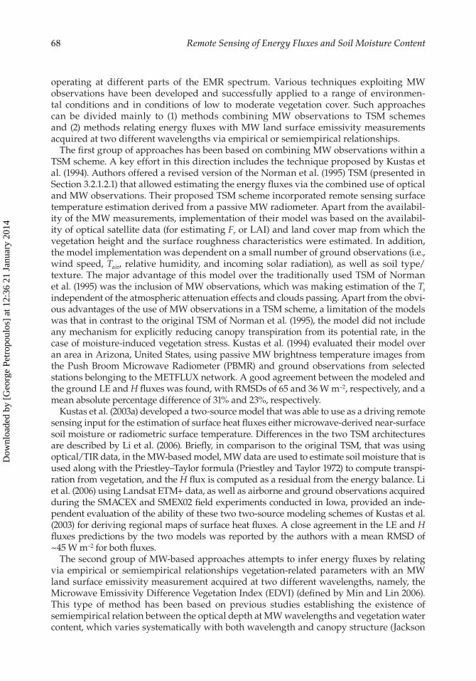
operating at different parts of the EMR spectrum. Various techniques exploiting MW observations have been developed and successfully applied to a range of environmen-tal conditions and in conditions of low to moderate vegetation cover. Such approaches can be divided mainly to (1) methods combining MW observations to TSM schemes and (2) methods relating energy fluxes with MW land surface emissivity measurements acquired at two different wavelengths via empirical or semiempirical relationships.
The first group of approaches has been based on combining MW observations within a TSM scheme. A key effort in this direction includes the technique proposed by Kustas et al. (1994). Authors offered a revised version of the Norman et al. (1995) TSM (presented in Section 3.2.1.2.1) that allowed estimating the energy fluxes via the combined use of optical and MW observations. Their proposed TSM scheme incorporated remote sensing surface temperature estimation derived from a passive MW radiometer. Apart from the availabil-ity of the MW measurements, implementation of their model was based on the availabil-ity of optical satellite data (for estimating Fr or LAI) and land cover map from which the vegetation height and the surface roughness characteristics were estimated. In addition, the model implementation was dependent on a small number of ground observations (i.e., wind speed, Tair, relative humidity, and incoming solar radiation), as well as soil type/ texture. The major advantage of this model over the traditionally used TSM of Norman et al. (1995) was the inclusion of MW observations, which was making estimation of the Ts independent of the atmospheric attenuation effects and clouds passing. Apart from the obvi-ous advantages of the use of MW observations in a TSM scheme, a limitation of the models was that in contrast to the original TSM of Norman et al. (1995), the model did not include any mechanism for explicitly reducing canopy transpiration from its potential rate, in the case of moisture-induced vegetation stress. Kustas et al. (1994) evaluated their model over an area in Arizona, United States, using passive MW brightness temperature images from the Push Broom Microwave Radiometer (PBMR) and ground observations from selected stations belonging to the METFLUX network. A good agreement between the modeled and the ground LE and H fluxes was found, with RMSDs of 65 and 36 W m–2, respectively, and a mean absolute percentage difference of 31% and 23%, respectively.
Kustas et al. (2003a) developed a two-source model that was able to use as a driving remote sensing input for the estimation of surface heat fluxes either microwave-derived near-surface soil moisture or radiometric surface temperature. Differences in the two TSM architectures are described by Li et al. (2006). Briefly, in comparison to the original TSM, that was using optical/TIR data, in the MW-based model, MW data are used to estimate soil moisture that is used along with the Priestley–Taylor formula (Priestley and Taylor 1972) to compute transpi-ration from vegetation, and the H flux is computed as a residual from the energy balance. Li et al. (2006) using Landsat ETM+ data, as well as airborne and ground observations acquired during the SMACEX and SMEX02 field experiments conducted in Iowa, provided an inde-pendent evaluation of the ability of these two two-source modeling schemes of Kustas et al. (2003) for deriving regional maps of surface heat fluxes. A close agreement in the LE and H fluxes predictions by the two models was reported by the authors with a mean RMSD of ~45 W m–2 for both fluxes.
The second group of MW-based approaches attempts to infer energy fluxes by relating via empirical or semiempirical relationships vegetation-related parameters with an MW land surface emissivity measurement acquired at two different wavelengths, namely, the Microwave Emissivity Difference Vegetation Index (EDVI) (defined by Min and Lin 2006). This type of method has been based on previous studies establishing the existence of semiempirical relation between the optical depth at MW wavelengths and vegetation water content, which varies systematically with both wavelength and canopy structure (Jackson
Dow
nloa
ded
by [
Geo
rge
Petr
opou
los]
at 1
2:36
21
Janu
ary
2014
69Remote Sensing of Surface Turbulent Energy Fluxes
and Schmugge 1991). As EDVI is directly linked to volumetric soil moisture content, the fast changes of EDVI represent canopy response to the changes of environmental condi-tions, such as water potential. EDVI values are derived from a combination of satellite MW measurements and optical as well as TIR observations. Min and Lin (2006) estimated the EDVI based on MW observations from the SSM/I sensor acquired over a forested region in the eastern United States and attempted to develop an empirical relationship relating EDVI to surface heat flux measurements acquired over the region concurrently to the satellite overpass. EDVI was found sensitive to EF fluxes, with a correlation coefficient (R) higher than 0.79 for cloudless conditions and higher than when NDVI was used in place of EDVI.
Li et al. (2009a) based on EDVI developed another algorithm for estimating EF and instantaneous LE fluxes from dense vegetation cover, by using the high temporal resolu-tion of EDVI. Investigators linked the seasonal trend of EDVI to the variance of canopy resistance due to the interrelationship among leaf development, environmental condition, and MW radiation. Li et al. (2009b) evaluated their algorithm using data from the same test site used by Min and Lin (2006) using also SSM/I satellite data. They reported a correlation coefficient (R) of 0.83 between the predicted and observed LE fluxes and bias and standard deviation of 3.31 and 79.63 W m–2, respectively. Authors pointed out as a key advantage of their approach that all key inputs required for its implementation could be replaced by satellite remote sensing and reanalysis data, which highlighted it as an important charac-teristic for a potential operational use of their method.
Min et al. (2010) developed and subsequently applied the EDVI for a region in the Amazon using satellite observations from the MW AMSR-E radiometers in combination with MODIS cloud products and reanalysis meteorological data from NCEP. Authors performed compari-sons for cloud-free days and reported that EDVI was able to capture vegetation variation from dense vegetation of the Amazon rainforest to the short/sparse vegetation of the savannah, under all-weather conditions. Also, in agreement to the previous findings by Min and Lin (2006), good correlations were found in their study between EDVI computed from the MW data and the optical indices such as the DVI and the Enhanced Vegetation Index (EVI), with an important advantage of EDVI being that it did not saturate in comparison to other indices.
All in all, MW-based remote sensing approaches are able to be applied under all-weather conditions, including cloudy days, which is an important advantage in comparison to other modeling schemes. Nevertheless, it should be noted that at present available passive MW imag-ing systems suitable for retrievals of soil moisture have spatial resolutions in the range of 35–65 km, which is much coarser than that of TIR radiometers that varies from 60 m with ASTER and Landsat to 5 km with the Geostationary Operational Environmental Satellite (GOES). Perhaps this is the main reason that explains their not so wide use and growth today in comparison to other approaches for modeling the surface fluxes from remote sensing observations.
3.3 Extrapolation Methods of the Instantaneous Estimates
Retrieval of regional estimates of surface heat fluxes from remote sensing has been largely based on deriving instantaneous estimates of those parameters at the time of satellite over-pass each time. However, for many practical applications (e.g., irrigation planning and water needs assessment), these instantaneous estimates can be indeed of very small use. A daytime or daily average LE or H flux estimate would be more interesting and simulta-neously useful in practice for use in hydrological and meteorological studies. This section
Dow
nloa
ded
by [
Geo
rge
Petr
opou
los]
at 1
2:36
21
Janu
ary
2014
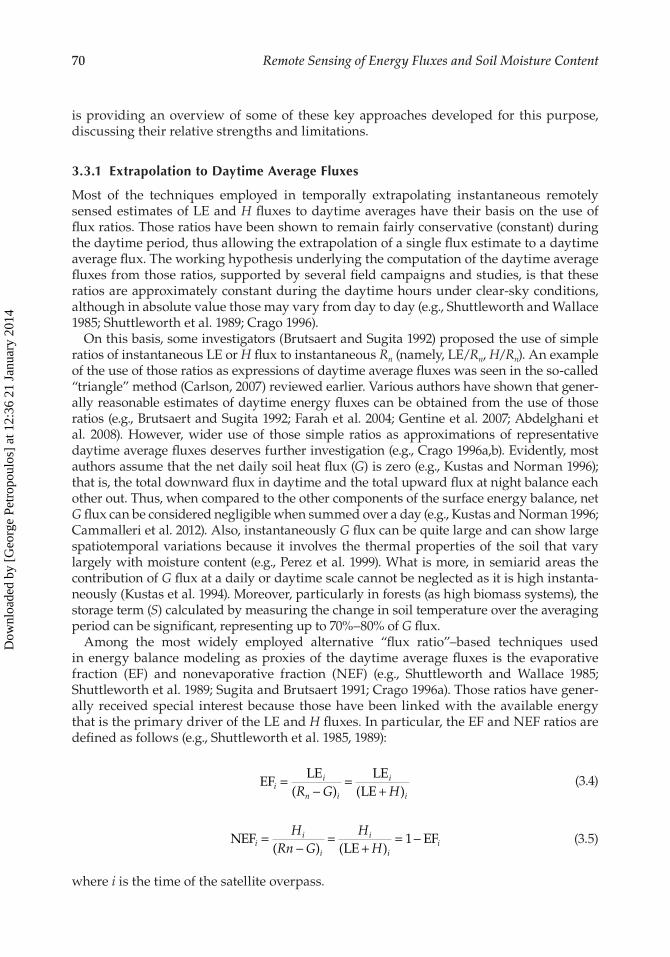
70 Remote Sensing of Energy Fluxes and Soil Moisture Content
is providing an overview of some of these key approaches developed for this purpose, discussing their relative strengths and limitations.
3.3.1 Extrapolation to Daytime Average Fluxes
Most of the techniques employed in temporally extrapolating instantaneous remotely sensed estimates of LE and H fluxes to daytime averages have their basis on the use of flux ratios. Those ratios have been shown to remain fairly conservative (constant) during the daytime period, thus allowing the extrapolation of a single flux estimate to a daytime average flux. The working hypothesis underlying the computation of the daytime average fluxes from those ratios, supported by several field campaigns and studies, is that these ratios are approximately constant during the daytime hours under clear-sky conditions, although in absolute value those may vary from day to day (e.g., Shuttleworth and Wallace 1985; Shuttleworth et al. 1989; Crago 1996).
On this basis, some investigators (Brutsaert and Sugita 1992) proposed the use of simple ratios of instantaneous LE or H flux to instantaneous Rn (namely, LE/Rn, H/Rn). An example of the use of those ratios as expressions of daytime average fluxes was seen in the so-called “triangle” method (Carlson, 2007) reviewed earlier. Various authors have shown that gener-ally reasonable estimates of daytime energy fluxes can be obtained from the use of those ratios (e.g., Brutsaert and Sugita 1992; Farah et al. 2004; Gentine et al. 2007; Abdelghani et al. 2008). However, wider use of those simple ratios as approximations of representative daytime average fluxes deserves further investigation (e.g., Crago 1996a,b). Evidently, most authors assume that the net daily soil heat flux (G) is zero (e.g., Kustas and Norman 1996); that is, the total downward flux in daytime and the total upward flux at night balance each other out. Thus, when compared to the other components of the surface energy balance, net G flux can be considered negligible when summed over a day (e.g., Kustas and Norman 1996; Cammalleri et al. 2012). Also, instantaneously G flux can be quite large and can show large spatiotemporal variations because it involves the thermal properties of the soil that vary largely with moisture content (e.g., Perez et al. 1999). What is more, in semiarid areas the contribution of G flux at a daily or daytime scale cannot be neglected as it is high instanta-neously (Kustas et al. 1994). Moreover, particularly in forests (as high biomass systems), the storage term (S) calculated by measuring the change in soil temperature over the averaging period can be significant, representing up to 70%–80% of G flux.
Among the most widely employed alternative “flux ratio”–based techniques used in energy balance modeling as proxies of the daytime average fluxes is the evaporative fraction (EF) and nonevaporative fraction (NEF) (e.g., Shuttleworth and Wallace 1985; Shuttleworth et al. 1989; Sugita and Brutsaert 1991; Crago 1996a). Those ratios have gener-ally received special interest because those have been linked with the available energy that is the primary driver of the LE and H fluxes. In particular, the EF and NEF ratios are defined as follows (e.g., Shuttleworth et al. 1985, 1989):
EF
LE LELEi
i
n i
i
iR G H=
−=
+( ) ( ) (3.4)
NEF
LEEFi
i
i
i
ii
HRn G
HH
=−
=+
= −( ) ( )
1 (3.5)
where i is the time of the satellite overpass.
Dow
nloa
ded
by [
Geo
rge
Petr
opou
los]
at 1
2:36
21
Janu
ary
2014
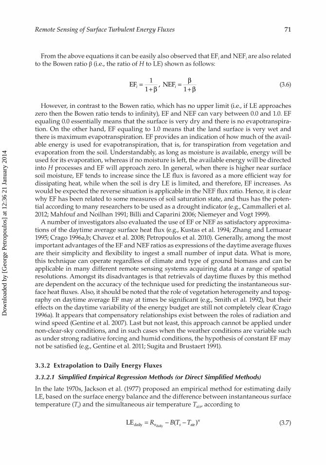
71Remote Sensing of Surface Turbulent Energy Fluxes
From the above equations it can be easily also observed that EFi and NEFi are also related to the Bowen ratio β (i.e., the ratio of H to LE) shown as follows:
EF NEFi i=
+=
+1
1 1ββ
β, (3.6)
However, in contrast to the Bowen ratio, which has no upper limit (i.e., if LE approaches zero then the Bowen ratio tends to infinity), EF and NEF can vary between 0.0 and 1.0. EF equaling 0.0 essentially means that the surface is very dry and there is no evapotranspira-tion. On the other hand, EF equaling to 1.0 means that the land surface is very wet and there is maximum evapotranspiration. EF provides an indication of how much of the avail-able energy is used for evapotranspiration, that is, for transpiration from vegetation and evaporation from the soil. Understandably, as long as moisture is available, energy will be used for its evaporation, whereas if no moisture is left, the available energy will be directed into H processes and EF will approach zero. In general, when there is higher near surface soil moisture, EF tends to increase since the LE flux is favored as a more efficient way for dissipating heat, while when the soil is dry LE is limited, and therefore, EF increases. As would be expected the reverse situation is applicable in the NEF flux ratio. Hence, it is clear why EF has been related to some measures of soil saturation state, and thus has the poten-tial according to many researchers to be used as a drought indicator (e.g., Cammalleri et al. 2012; Mahfouf and Noilhan 1991; Billi and Caparini 2006; Niemeyer and Vogt 1999).
A number of investigators also evaluated the use of EF or NEF as satisfactory approxima-tions of the daytime average surface heat flux (e.g., Kustas et al. 1994; Zhang and Lemuear 1995; Crago 1996a,b; Chavez et al. 2008; Petropoulos et al. 2010). Generally, among the most important advantages of the EF and NEF ratios as expressions of the daytime average fluxes are their simplicity and flexibility to ingest a small number of input data. What is more, this technique can operate regardless of climate and type of ground biomass and can be applicable in many different remote sensing systems acquiring data at a range of spatial resolutions. Amongst its disadvantages is that retrievals of daytime fluxes by this method are dependent on the accuracy of the technique used for predicting the instantaneous sur-face heat fluxes. Also, it should be noted that the role of vegetation heterogeneity and topog-raphy on daytime average EF may at times be significant (e.g., Smith et al. 1992), but their effects on the daytime variability of the energy budget are still not completely clear (Crago 1996a). It appears that compensatory relationships exist between the roles of radiation and wind speed (Gentine et al. 2007). Last but not least, this approach cannot be applied under non-clear-sky conditions, and in such cases when the weather conditions are variable such as under strong radiative forcing and humid conditions, the hypothesis of constant EF may not be satisfied (e.g., Gentine et al. 2011; Sugita and Brustaert 1991).
3.3.2 Extrapolation to Daily Energy Fluxes
3.3.2.1 Simplified Empirical Regression Methods (or Direct Simplified Methods)
In the late 1970s, Jackson et al. (1977) proposed an empirical method for estimating daily LE, based on the surface energy balance and the difference between instantaneous surface temperature (Ts) and the simultaneous air temperature Tair, according to
LEdaily airdaily
= − −R B T Tn sn( ) (3.7)
Dow
nloa
ded
by [
Geo
rge
Petr
opou
los]
at 1
2:36
21
Janu
ary
2014
72 Remote Sensing of Energy Fluxes and Soil Moisture Content
where B and n are the site-specific regression coefficients dependent on surface roughness, wind speed, atmospheric stability, etc. (Li et al. 2009b), which are determined either by lin-ear least squares fit to data or by simulations based on a SVAT model (Carlson and Buffum 1989; Carlson et al. 1995).
The principal assumptions on which the method of operation is based include the fact that G flux is negligible when considering the daily estimation of LE fluxes, and also that the ratio of H/Rn is also constant during daytime. Details on this method foundation can be found, for example, in the work of Seguin and Itier (1983), whereas the implications of the regression coefficients in the simplified equation are discussed by Carlson et al. (1995). In Equation 3.7, Rn and Ts are computed in a relatively straightforward way from optical and thermal data, whereas the estimation of Tair is perhaps the most problematic to be acquired. The latter can be estimated in different ways, including geostatistical interpola-tion methods of meteorological observations or using empirical relationships with VIs (see review by Courault et al. 2005).
Various studies have evaluated the above equation, confirming its potential use as a simple method for deriving coarse estimates of daily LE fluxes under a variety of atmospheric conditions and vegetation covers (Carlson and Buffum 1989; Carlson et al. 1995; Tsouni et al. 2008; Delogu et al. 2012). Generally, those studies have shown that error in the predicted daily LE fluxes by the Jackson et al. (1977) method is about 1 mm day–1. Also, a number of refinements of the Jackson et al. (1977) equation have been proposed over the years. Some schemes have been based on parameterizations of the B and n coefficients as a function of wind speed, roughness, and criterions of atmospheric stability (Vidal and Perrier 1989; Lagouarde and McAneney 1992). For example, Carlson and Buffum (1989) used the simplified equation that might be more applicable to regional-scale ET estimations if the air temperature and wind speed were measured or evaluated at a level of 50 m, owing to the fact that at this height varia-tion of the meteorological parameters, they are assumed to be insensitive to surface characteristics.
Generally, key advantages of the simplified empirical regression methods include their ease and straightforward implementation along with their low demand in data provision. Also, these methods are offering relatively sufficient accuracy in the estimation of daily evapotranspiration values from a very small number of ground-measured variables. What is more, those modeling approaches do not require estimates of instantaneous energy fluxes to be computed previously and thus are not affected by the accuracy of the instantaneous LE and H flux estimation (as is the case with other approaches discussed next). The need for local calibration of the empirical coefficients is perhaps the single most important disadvantage to be taken under consideration in using those practically. Parameters such as the surface roughness and wind speed cannot be directly provided by remote sensing, and this perhaps is the main reason limiting their use so far (see Li et al. 2009b). Besides, most of these methods are based on the assumption that the Tair and Rn are not spatially varying, which can be valid only if canopy albedo and surface temperature do not vary significantly, which is not always the case especially under very heterogeneous surfaces.
3.3.2.2 EF-Based Methods
A widely used approach employed for the temporal extrapolation of instantaneous LE fluxes to daily values has been related to the EF introduced earlier in Section 3.1. On the basis of the EF concept of Shuttleworth et al. (Shuttleworth and Wallace 1985; Shuttleworth
Dow
nloa
ded
by [
Geo
rge
Petr
opou
los]
at 1
2:36
21
Janu
ary
2014
73Remote Sensing of Surface Turbulent Energy Fluxes
et al. 1989), Sugita and Brutsaert (1991) introduced the idea of the use of this ratio for deriv-ing daily totals of evapotranspiration rates from corresponding instantaneous estimates. In particular, the authors suggested that the daytime evapotranspiration could be calcu-lated from
LEd = EFeQd (3.8)
where EFe is the evaporative fraction determined from one or more instantaneous flux values and Qd is the total daytime available energy, determined as
Q R G td n
t
t
= −∫ ( )d
2
1
(3.9)
where Rn is the net radiation and G is the ground heat flux, (t2 − t1) represents the time daylight period defined as the time of day when (Rn − G) is greater than or equal to zero. EF is computed as
EF
LE
LEe
i
i
n
i i
i
n
H
=
+
∑∑( )
(3.10)
where the subscript i refers to the ith measurement and n is the total number of daytime measurements.
Therefore, to calculate daily total LE from Equation 3.7, it is necessary to determine the EF term, which can be obtained using remote sensing data and the daytime total available energy, as described earlier (Section 3.1). This method is very easy and straightforward to be applied, and these are its key advantages. The main downsides are the requirement for more than one instantaneous EF estimate and that of daytime total available energy. Also, the accuracy of the daily evapotranspiration fluxes will depend on the accuracy of the instantaneous LE and H fluxes and the method cannot be applied on cloudy days.
Others (e.g., Kustas et al. 1994; Sarwar and Bill 2007) have proposed the retrievals of daily LE fluxes from the midday EF based on the following equation:
LE EFdaily midday daily
= ⋅ +0 0345. Rn (3.11)
where Rndaily is the daily net radiation (W m–2) and 0.0345 is a conversion factor. The daily net radiation is computed, using standard meteorological data as follows:
R K
KKndaily
exo
= − ↓ − ↓↓
( )1 110α (3.12)
where α is the surface albedo, K↓ is the global radiation at the surface level, and Kexo↓ is the theoretical extraterrestrial radiation.
Dow
nloa
ded
by [
Geo
rge
Petr
opou
los]
at 1
2:36
21
Janu
ary
2014
74 Remote Sensing of Energy Fluxes and Soil Moisture Content
Another variant of the EF-based method in temporally extrapolating the instantaneous energy fluxes to daily total energy fluxes is employed in the SEBS model reviewed earlier (see Section 3.2.1.1), in which the daily LE flux can be determined as
LE EFdaily = ⋅ ⋅ ⋅ −
8 64 107.R Gn
wλρ (3.13)
where LEdaily is the actual LE flux on a daily basis (mm day–1), EF is the daily average EF, which is approximated by SEBS, Rn
and G are the daily net radiation and soil heat flux, respec-tively, λ is the latent heat of vaporization (J kg–1), and ρw is the density of water (kg m–3). In SEBS, since the daily G flux is close to zero because the downward flux in the daytime and the upward flux at night balance each other approximately, the daily LE flux depends only on the total net radiation flux, which in SEBS is computed as
R K Ln = − ⋅ + ⋅↓( )1 24 24α ε (3.14)
where K24↓ is the daily incoming global radiation, L24 is the daily net longwave radiation, α
is the daily average albedo, and ε is the emissivity.In SEBAL, estimation of the daily LE fluxes is also based on the EF concept, where the
daily LE flux is also linked to EF, as follows:
LE EFdaily daily
= ⋅ ⋅ ⋅86400 103
λρwnR (3.15)
where Rndaily is the 24 h averaged daily Rn, λ is the latent heat of vaporization (J kg–1), ρw is
the density of water (kg m–3), and LEdaily is expressed in mm day–1.
3.3.2.3 Sinusoid Relationship
On the basis of the assumption that the diurnal course of LE generally follows the course of solar radiation throughout the daylight period, Jackson et al. (1983) demonstrated that the ratio of total solar radiation to an instantaneous value taken during midday could be approximated by a sine function. On the basis of this finding, the authors proposed the computation of the daily total LE flux from an instantaneous LE estimate and a conversion coefficient given as a function of latitude, day of year, and time of day. More specifically, according to Jackson et al. (1983), the instantaneous solar irradiance (Si) on a clear day can be approximated as
S S
tNi m=
sinπ (3.16)
where Sm is the maximum irradiance at solar noon, t is the time beginning at sunrise, and N is the time period between sunrise and sunset in units of t. Integration of Equation 3.16 yields the daily total irradiance Sd:
Dow
nloa
ded
by [
Geo
rge
Petr
opou
los]
at 1
2:36
21
Janu
ary
2014
75Remote Sensing of Surface Turbulent Energy Fluxes
S St
Nt N Sd m m
N
=
= ( )∫ sinπ
πd 2
0
(3.17)
Therefore the ratio of total daily irradiance to the instantaneous irradiance at time t is given by
J S
SN
t Nd
i= = 2
[ sin( )]π π / (3.18)
where t and N in the argument of the sine function must have the same units. The daylight period N can be expressed by
N = 0.945 ⋅ [α + b sin2[π(D + 10)/365]] (3.19)
where a and b are latitude-dependent constants; the constant a represents the shortest day-light period of the year and the constant b is the amount that must be added to a in order to obtain the longest daylight of the year; and D is the day of the year. The constants a and b can be calculated as a function of latitude (Jackson et al. 1983):
α = 12.0 − 5.69 ⋅ 10−2 L − 2.02 ⋅ 10−4 L2 + 8.25 ⋅ 10−6 L3 − 3.15 ⋅ 10−7 L4 (3.20)
b = 0.123 ⋅ L − 3.10 ⋅ 10−4 L2 + 8.00 ⋅ 10−7 L3 + 4.99 ⋅ 10−7 L4 (3.21)
where L is the latitude in degrees.Using the similarity between the diurnal course of evapotranspiration and the one of
solar irradiance, daytime LE can be estimated as
LE LE
/d id
iiE S
SN
t N=
=
2π πsin(
(3.22)
where LEd is the daytime evapotranspiration in MJ m2 day–1 and LEi is the instantaneous evapotranspiration in W m–2, which can be obtained from the energy balance equation using EO data. The method also requires the conversion coefficient (J), which is a simple function of latitude, day of year, and time of day.
Jackson et al. (1983) evaluated the above approach and showed a strong correlation between measured and estimated daily LE fluxes. For example, Zhang and Lemeur (1995), in a comparison of different methods for the daily estimation of LE fluxes for cloud free days using data from the HAPEX-MOBIHLY experiment in France, reported comparable results in the predicted daily LE fluxes between the method of Jackson et al. (1983) and the EF method of Sugita and Brutsaert (1991). An important advantage of the Jackson et al. (1983) method for potential operational implementation is that it requires only one instan-taneous value of evapotranspiration and the conversion coefficient, which is a function of latitude and the day of year. In contrast, the Sugita and Brutsaert (1991) method requires more than one instantaneous EF fraction and daytime total available energy values in deriving the daily LE fluxes.
Dow
nloa
ded
by [
Geo
rge
Petr
opou
los]
at 1
2:36
21
Janu
ary
2014
76 Remote Sensing of Energy Fluxes and Soil Moisture Content
On the basis of the same concept, Xie (1999) suggested the transformation of the instan-taneous LE flux to daily LE fluxes based on the sinusoid relationship between daily and instantaneous LE fluxes, as follows:
LELE /
d E
E
Nt N
= 2π πsin( )
(3.23)
where LEd is the daily LE flux, LE is the instantaneous LE flux, t is the time of satellite sen-sor overpass, and NE is the daily hours, which can be calculated by minus two from the daily sunshine hours.
Various investigators have applied the above method in arid and semiarid regions using different types of remote sensing data, reporting generally satisfactory results in daily LE predictions. For example, Yunhao et al. (2003) compared daily LE fluxes derived by the Xie (1999) method for a region in China derived from Advanced Very High Resolution Radiometer (AVHRR) observations and reported a generally satisfactory agreement with the corresponding ground measurements with an average relative error of 16% and R2 of 0.77. The latter scheme or variants of it has been widely applied today by many in deriving daily LE flux estimates (e.g., Zhang et al. 2006; Liu et al. 2010).
3.4 Conclusions and Future Outlook
This chapter presented an overview of the most widely approaches employed key meth-odologies employed in deriving spatiotemporal estimates of LE and H fluxes from remote sensing. It can be concluded that remote sensing–based estimation of energy fluxes is per-formed in quite diverse, unconnected ways. Our review showed that an average RMSD value of about 50 W m–2 and relative error of 15%–30% in the estimation of LE and H fluxes by remote sensing is expected to be found by many techniques. Taking into account that an absolute accuracy of ~50 W m–2 in energy fluxes is generally considered satisfactory for a large range of applications, it is clear that EO technology is showing a promising poten-tial in this direction.
From an algorithmic point of view, nearly all available methods in deriving estimates of LE and H fluxes have been developed essentially for cloud-free conditions. What is more, for the majority of the techniques employed, thermal remote sensing data consist of one of the most crucial inputs required, together with optical data. Also, interestingly, a survey of the different methods showed that more multifaceted physical and analytical model-ing approaches do not necessarily provide more accurate energy fluxes retrievals than, for example, more empirically based techniques. Indeed, the different groups of meth-ods reviewed are characterized by different strengths and limitations. Evidently, more work is required to address some of the key limitations imposed in obtaining more accu-rate retrievals of energy fluxes from space and even more to put forward an operational implementation scenario in the retrievals of those parameters at a global scale. Actually, several approaches at present investigate the perspective of global operational estimation of energy fluxes by remote sensing. Along these lines are, for example, the ESA-funded WACMOS and PROgRESSIon (European Space Agency 2012) projects, which explore the
Dow
nloa
ded
by [
Geo
rge
Petr
opou
los]
at 1
2:36
21
Janu
ary
2014
77Remote Sensing of Surface Turbulent Energy Fluxes
development of a series of prototype products from the synergy of remote sensing observa-tions acquired from different ESA-funded missions.
Given the limitations inherent to both sensing systems and modeling approaches, it is clear that it will be necessary to direct efforts toward the investigation of the potential added value from the exploitation of the synergistic use of remote sensing systems and/or modeling approaches. The data and technique complementarity (independent infor-mation) and interchangeability (similar information) will assist in developing approaches that better address aspects currently unsolved, such as the spatial and temporal resolu-tion or land surface heterogeneity. In addition, intercomparison studies between different modeling approaches at dissimilar ecosystem conditions, such as those currently imple-mented in the framework of the LandFLux GEOWEX project, should be further fostered. Such initiatives will allow one to not only appreciate the relative strengths and limitations between the models but also appreciate their prediction accuracy under different eco-system conditions globally. To this end, the availability of relevant ground observations from global networks such as the FLUXNET and CarboEurope, which are able to provide systematically long-term measurements of relevant land surface parameters, should be continuously supported. This is important, as such data assist not only in validating sat-ellite-derived and modeling results but also in better understanding the relevant physical processes that occurred at different scales of observation using EO data.
Last but not least, the recent launch of remote sensing radiometers such as that of Landsat 8 and the forthcoming launch of SENTINELS 2/3 will continue the heritage of thermal infrared observations from space. It is also expected to foster the development of new modeling techniques for improving the retrieval accuracy of energy fluxes from EO technology. Yet, this prospect remains to be seen in years to come.
Acknowledgments
This work was produced in the framework of the PROgRESSIon (Prototyping the Retrievals of Energy Fluxes and Soil Moisture Content) project implementation, funded by the European Space Agency (ESA) Support to Science Element (STSE) under contract STSE-TEBM-EOPG-TN-08-0005. Dr. Petropoulos gratefully acknowledges the financial support provided by the Agency.
References
Abdelghani, C., J. C. B. Hoedjes, J.-C. Rodriquez, C. J. Watts, J. Gatatuza, F. Jacob, and Y. H. Kerr (2008): Using remotely sensed data to estimate area-averaged daily surface fluxes over a semi-arid mixed agricultural land, Agric. For. Meteorol., 148, 330–342.
Allen, R. G., M. Tasumi, A. Morse, R. Trezza, J. L. Wright, W. Bastiaanssen, W. Kramber, I. J. Lorite, and C.W. Robison (2007): Satellite-based energy balance for mapping evapotranspiration with internalized calibration (METRIC)—Applications, J. Irrig. Drain. Eng., 133(4), 395–406.
Anderson, M. C., J. M. Norman, G. R. Diak, and W. P. Kustas (1997): A two-source time Integrated model for estimating surface fluxes for thermal infrared satellite observations, Remote Sens. Environ., 60, 195–216.
Dow
nloa
ded
by [
Geo
rge
Petr
opou
los]
at 1
2:36
21
Janu
ary
2014
78 Remote Sensing of Energy Fluxes and Soil Moisture Content
Anderson, M. C., J. M. Norman, W. P. Kustas, R. Houborg, P. J. Starks, and N. Agam (2008): A thermal-based remote sensing technique for routine mapping of land surface carbon, water and energy fluxes from field to regional scales, Remote Sens. Environ., 112, 4227–4241.
Anderson, M. C., W. P. Kustas, J. M. Noorman, C. R. Hain, J. R. Mecikalski, L. Schultz, M. P. Gonzalez-Dugo et al. (2010): Mapping daily evapotranspiration at field to global scales using geostation-ary and polar orbiting satellite imagery, Hydrol. Earth Syst. Sci. Discuss., 7, 5957–5990.
Arthur-Hartanft, T., T. N. Carlson, and K. C. Clarke (2003): Satellite and ground-based microclimate and hydrologic analyses coupled with a regional urban growth model, Remote Sens. Environ., 86, 385–400.
Asrar, G. (1989): Theory and Applications of Optical Remote Sensing, John Wiley, New York.Bashir, M. A., T. Hata, H. Tanakamaru, A. W. Abdelhadi, and A. Tada (2008): Satellite-based energy
balance model to estimate seasonal evapotranspiration for irrigated sorgum: A case study from the Gezira scheme, Sudan, Hydrol. Earth Syst. Sci., 12, 1129–1139.
Bastiaanssen, M. D. (2000): SEBAL-land based sensible and latent heat fluxes in the irrigated Gediz Basin, Turkey, J. Hydrol., 229, 87–100.
Bastiaanssen, W. G. M. (1995): Regionalisation of surface flux densities and moisture indicators in composite terrain. PhD Thesis, Wageningen, Agricultural University, the Netherlands: 273 pp.
Bastiaanssen, W. G. M., E. J. M. Noordman, H. Pelgrum, G. Davids, B. P. Thoreson, and R. G. Allen (2005): SEBAL model with remotely sensed data to improve water-resources management under actual field conditions, J. Irrig. Drain. Eng., 131(1), 85–93.
Bastiaanssen, W. G. M., M. Menenti, R. A. Feddes, and A. A. M. Holstag (1998): A remote sensing surface energy balance algorithm for land (SEBAL): 1. Formulation, J. Hydrol., 198–212.
Batra, N., S. Islam, V. Venturini, G. Bisht, and L. Jiang (2006): Estimation and comparison of evapo-transpiration from MODIS and AVHRR for clear sky days over the Southern Great Plains, Remote Sens. Environ., 103, 1–15.
Battrick, B. (2006): The changing Earth: New scientific challenges for ESA’s Living Planet Programme, Eur. Space Agency Spec. Publ., ESA SP-1304.
Bhattacharya, B. K., K. Mallick, and J. S. Parihar (2010): Regional clear sky evapotranspiration over agricultural land using remote sensing data from Indian geostationary meteorological satellite, J. Hydrol., 387, 65–80.
Billi, P., and F. Caparrini (2006): Estimating land cover effects on evapotranspiration with remote sensing: a case study in Ethiopian Rift valley, Hydrol. Sci., 51(4), 655–668.
Brunsell, N. A., and R. R. Gillies (2003): Scale issues in land-atmosphere interactions: Implications for remote sensing of the surface energy balance, Agric. For. Meteorol., 117, 203–221.
Brutsaert, W., and M. Sugita (1992): Application of self-preservation in the diurnal evolution of the surface energy budget to determine daily evaporation, J. Geophys. Res., 97, D17, 18377–18382.
Calvet, J. C., J. Noilhan, and P. Bessemoulin (1998): Retrieving the root zone soil moisture from sur-face soil moisture or temperature estimates: A feasibility study based on field measurements, J. Appl. Meteorol., 37, 371–386.
Cammalleri, C., G. Ciraolo, G. La Loggia, and A. Maltese (2012): Daily evapotranspiration assess-ment by means of residual surface energy balance modeling: A critical analysis under a wide range of water availability, J. Hydrol., 452–453(C), 119–129.
Caparrini, F., F. Castelli, and D. Entekhabi (2003): Mapping of land-atmosphere heat fluxes and sur-face parameters with remote sensing data, J. Hydrometeorol., 5, 145−159.
Carlson, T. N. (2007): An overview of the “triangle method” for estimating surface evapotranspira-tion and soil moisture from satellite imagery, Sensors, 7, 1612–1629.
Carlson, T. N., and M. J. Buffum (1989): On estimating total daily evapotranspiration from remote surface temperature measurements, Remote Sens. Environ., 29, 197–207.
Carlson, T. N., W. J. Capehart, and R. R. Gilies (1995): A new look at the simplified method for remote sensing of daily evapotranspiration, Remote Sens. Environ., 54, 161–167.
Chavez, J. L., and C. M. U. Neale (2003): Validating airborne multispectral remotely sensed heat fluxes with ground energy balance tower and heat flux source area (footprint) functions. ASAE Paper No. 033128. St. Joseph, Michigan.
Dow
nloa
ded
by [
Geo
rge
Petr
opou
los]
at 1
2:36
21
Janu
ary
2014
79Remote Sensing of Surface Turbulent Energy Fluxes
Chavez, J. L., C. M. U. Neale, L. E. Hipps, J. H. Prueger, and W. P. Kustas (2005): Comparing aircraft-based remotely sensed energy balance fluxes with eddy covariance tower data using heat flux source area functions, J. Hydrometeorol., 6, 923–940.
Chavez, J. L., C. M. U. Neale, J. H. Prueger, and W. P. Kustas (2008): Daily evapotranspiration esti-mates from extrapolating instantaneous airborne remote sensing ET values, Irrig. Sci., 27, 67–81.
Chavez, J. L., P. H. Gowda, T. A. Howell, and K. Copeland (2009): Radiometric surface temperature calibration effects on satellite based evapotranspiration estimation, Int. J. Remote Sens., 30(9), 2337–2354.
Chen, J.-H., C.-E. Kan, C.-H. Tan, and S.-F. Shih (2002): Use of spectral information for wetland evapotranspiration assessment, Agric. Water Manag., 55, 239–248.
Courault, D., P. Clastre, P. Cauchi, and R. Del´ecolle (1998): Analysis of spatial variability of air tem-perature at regional scale using remote sensing data and a SVAT model, In Proceedings of the First International Conference on Geospatial Information in Agriculture and Forestry, vol. II, ERIM International, Ann Arbor, Mich.
Courault, D., B. Sequin, and A. Olioso (2005): Review on estimation of evapotranspiration from remote sensing data: From empirical to numerical modeling approaches, Irrig. Drain. Syst., 19, 223–249.
Courtier, P., E. Andersson, W. Heckley, J. Pailleux, D. Vasiljevic, M. Hamrud, A. Hollingsworth et al. (1998): The ECMWF implementation of three-dimensional variational assimilation (3D-Var). I: Formulation, Q. J. R. Meteorol. Soc., 124, 1783–1807.
Crago, R. D. (1996a): Conservation and variability of the evaporative fraction during the daytime, J. Hydrol., 180, 173–194.
Crago, R. D. (1996b): Daytime evaporation from conservation of surface flux ratios. In Scaling Up in Hydrology Using Remote Sensing, Chapter 16. John Wiley, New York.
Crow, W. T., and W. P. Kustas (2005): Utility of assimilating surface radiometric temperature observa-tions for evaporative fraction and heat transfer coefficient retrieval, Boundary Layer Meteorol., 115, 105–130.
Delogu, E., G. Boulet, A. Olioso, B. Coudert, J. Chirouze, E. Ceschia, V. Le Dantec et al. (2012): Reconstruction of temporal variations of evapotranspiration using instantaneous estimates at the time of satellite overpass, Hydrol. Earth Syst. Sci., 16(8), 2995–3010.
Diak, G., J. R. Mecikalski, M. C. Anderson, J. M. Norman, W. P. Kustas, R. D. Torn, and R. L. Dewolf (2004): Estimating land surface energy budgets from space: Review and current efforts at the University of Wisconsin-Madison and USDA-ARS, Bull. Am. Meteorol. Soc., 65–78, doi: 10.1175/BAMS-85-1-65.
European Space Agency (2012): Prototyping the retrievals of energy fluxes and soil surface mois-ture. Available at http://due.esrin.esa.int/stse/projects/stse_project.php?id=148 (Accessed on November 24, 2012).
Farah, H. O., W. G. M. Bastiaanssen, and R. A. Feddes (2004): Evaluation of the temporal variability of the evaporative fraction in a tropical watershed, Int. J. Appl. Earth Obs. Geoinf., 5, 129–140.
French, A., T. Schmugge, and W. P. Kustas (2002): Estimating evapotranspiration over El-Reno, Oklahoma with ASTER imagery, Agronomie, 22, 105–106.
Gentine, P., D. Entekhabi, A. Chehbouni, G. Boulet, and B. Duchemin (2007): Analysis of evaporative fraction diurnal behaviour, Agric. For. Meteorol., 143, 13–29.
Gentine, P., D. Entekhabi, and J. Polcher (2011), The diurnal behavior of evaporative fraction in the soil-vegetation-atmospheric boundary layer continuum, J. Hydrometeorol., 12(6), 1530–1546, doi:10.1175/2011JHM1261.1.
Gillespie, A., S. Rokugawa, T. Mantsunaga, J. S. Cothern, S. Hook, and A. Kahle (1998): A temper-ature and emissivity separation algorithm for Advanced Spaceborne Thermal Emission and Reflection Radioemeter (ASTER) images, IEEE Trans. Geosci. Remote Sens., 36, 1113–1126.
Gillies, R. R., T. N. Carlson, J. Cui, W. P. Kustas, and K. S. Humes, (1997): Verification of the “triangle” method for obtaining surface soil water content and energy fluxes from remote measurements of the Normalized Difference Vegetation Index NDVI and surface radiant temperature, Int. J. Remote Sens., 18, 3145–3166.
Dow
nloa
ded
by [
Geo
rge
Petr
opou
los]
at 1
2:36
21
Janu
ary
2014
80 Remote Sensing of Energy Fluxes and Soil Moisture Content
Glenn, E., A. R. Huete, P. L. Nagler, K. K. Hirschboeck, and P. Brown (2007): Integrating remote sens-ing and ground methods to estimate evapotranspiration, Crit. Rev. Plant Sci., 26, 139–168.
Gomez, M., A. Olioso, J. A. Sobrino, and F. Jacob (2005): Retrieval of evapotranspiration over the Aplilles/ReSeDA experimental site using airborne POLDER sensor and a thermal camera, Remote Sens. Environ., 96, 399–408.
Gonzalez-Dugo, M. P., C. M. U. Neale, L. Mateos, W. P. Kustas, J. H. Prueger, M. C. Anderson, and F. Li (2009): A comparison of operational remote sensing-based models for estimating crop evapo-transpiration, Agric. Forest. Meteorol., 149, 1843–1853.
Gowda, P. H., J. L. Chavez, T. A. Howell, T. H. Marek, and L. L. New (2008): Surface energy balance based evapotranspiration mapping in the Texas High plains, Sensors, 8, 5186–5201.
Hasager, C., and N. O. Jensen (1999): Surface-flux aggregation in heterogeneous terrain, Q. J. R. Meteorol. Soc., 125, 267–284.
Jackson A. C., J. P. Butler, E. J. Millet, F. G. Hoppin, and S. V. Dawson (1977): Airway geometry by analysis of acoustic pulse response measurements, J. Appl. Physiol., 43(3), 523–536.
Jackson, R. D., J. L. Hatfield, R. J. Reginato, S. B. Idso, and P. J. Pinter (1983): Estimation of daily evapotranspiration from one time-of-day measurements, Agric. Water Manage., 7, 351–362.
Jackson, R. D., D. B. Idso, R. J. Reginato, and P. J. Pinter (1981): Canopy temperature as a crop water stress indicator, Water Resour. Res., 17, 1133–1138.
Jackson, T., and T. Schmugge (1991): Vegetation effects on the microwave emission of soils, Remote Sens. Environ., 36, 203–212.
Jiang, L., and S. Islam (1999): A methodology for estimation of surface evapotranspiration over large areas using remote sensing observations, Geophys. Res. Lett., 26, 2773–2776.
Jiang, L., and S. Islam (2001): Estimation of surface evaporation map over Southern Great Plains using remote sensing data, Water Resour. Res., 37, 329–340.
Jiang, L., and S. Islam (2003): An intercomparison of regional heat flux estimation using remote sens-ing data, Int. J. Remote Sens., 24, 2221–2236.
Jordan, J. D. and S. F. Shih (2000): Satellite-based diurnal and seasonal thermal patterns of natu-ral, agricultural, and urban land-cover vs. soil type in Florida. In Proceedings of the 2nd International Conference on Geospatial Information in Agriculture and Forestry (ICGIAF), vol. I. ERIM International, Ann Arbor, Mich., pp. 489–495.
Kalma, J. D., T. R. McVicar, and M. F. McCabe (2008): Estimating land surface evaporation: A review of methods using remotely sensed surface temperature data, Surv. Geophys., 29(4–5), 421–469.
Khan, S. I., Y. Hong, B. Vieux, and W. Liu (2010): Development and evaluation of an actual evapo-transpiration estimation algorithm using satellite remote sensing and meteorological observa-tional network in Oklahoma, Int. J. Remote Sens., 31(14), 3799–3819.
Kongo, M. V., G. W. P. Gewitt, and S. A. Lorentz (2011): Evaporative water use of different land uses in the upper-Thukela river basin assessed from satellite imagery, Agric. Water Manage., 98(11), 1727–1739.
Kustas, W. P., A. N. French, J. L. Hatfield, T. J. Jackson, M. S. Moran, A. Rango, J. C. Ritchie et al. (2003) Remote sensing research in hydrometeorology, Photogramm. Eng. Remote Sens., 69(6), 631–646.
Kustas, W. P., D. C. Goodrich, M. S. Moran, S. A. Amer, L. B. Bach, J. H. Blanford, A. Chehbouni et al. (1991): An interdisciplinary field study of the energy and water fluxes in the atmosphere-biosphere system over semi-arid rangelands: Description and some preliminary results, Bull. Am. Meteorol. Soc., 72, 1683–1705.
Kustas, W. P., J. Hatfield, and J. H. Prueger (2005): The Soil Moisture–Atmosphere Coupling Experiment (SMACEX): Background, hydrometerological conditions, and preliminary find-ings, J. Hydrometerol., 6, 791–804.
Kustas, W. P., M. S. Moran, K. S. Humes, D. I. Stannard, P. J. Pinter, Jr., L. E. Hipps, E. Swiatek, and D. C. Goodrich (1994): Surface energy balance estimates at local and regional scales using opti-cal remote sensing from an aircraft platform and atmospheric data collected over semiarid rangelands, Water Resour. Res., 30(5), 1241–1259.
Kustas, W., J. M. Norman, M. C. Anderson, and A. N. French (2003): Estimating subpixel surface tem-peratures and energy fluxes from the vegetation index–radiometric temperature relationship, Remote Sens. Environ., 85, 429–440.
Dow
nloa
ded
by [
Geo
rge
Petr
opou
los]
at 1
2:36
21
Janu
ary
2014
81Remote Sensing of Surface Turbulent Energy Fluxes
Kustas, W. P., and J. M. Norman (1996): Use of remote sensing for evapotranspiration monitoring over land surfaces, Hydrol. Sci. J., 41, 495–516.
Lagouarde, J. P., and K. J. McAneney (1992): Daily sensible heat flux estimation from a single mea-surement of surface temperature and maximum air temperature, Boundary Layer Meteorol., 59(4), 341–362.
Li, F., and T. J. Lyons (1998): Estimation of regional evapotranspiration through remote sensing, J. Appl. Meteorol., 38, 1644–1654.
Li, F., W. P. Kustas, M. C. Anderson, T. J. Jackson, R. Bindlish, and J. H. Prueger (2006): Comparing the utility of microwave and thermal remote sensing constrains in two-source energy balance modelling over an agricultural landscape, Remote Sens. Environ., 101, 315–328.
Li, F., W. P. Kustas, M. C. Anderson, J. H. Prueger, and R. L. Scott (2008): Effect of remote sensing spa-tial resolution on interpreting tower-based flux observations, Remote Sens. Environ., 112, 337–349.
Li, R., Q. Min, and B. Lin (2009a): Estimation of evapotranspiration in a mid-latitude forest using the Microwave Emissivity Difference Vegetation Index (EDVI), Remote Sens. Environ., 113, 2011–2018.
Li, Z.-L., R. Tang, Z. Wan, Y. Bi, C. Zou, B. Tang, G. Yan, and X. Zhang (2009b): A review of current methodologies for regional evapotranspiration estimation from remotely sensed data, Sensors, 9, 3801–3852.
Liu, R., J. Wen, X. Wang, L. Wang, H. Tian, T. T. Zhang, X. K. Shi., J. H. Zhang, and S. H. N. Lv (2010): Actual daily evapotranspiration estimated from MERIS and AATSR data over the Chinese Loess Plateau, Hydrol. Earth Syst. Sci., 14, 47–58.
Ma, W., Y. Ma, Z. Su, J. Wang, and H. Ishikawa (2011): Estimating surface fluxes over middle and upper streams of the Heihe river basin with ASTER imagery, Hydrol. Earth Sci., 15, 1403–1413.
Mahfouf, J. F., and J. Noilhan (1991): Comparative study of various formulations of evaporation from bare soil using in situ data, J. Appl. Meteorol., 30, 1354–1365.
Margulis, S. A., and D. Entekhabi (2003): Variational assimilation of radiometric surface temperature and reference-level micrometeorology into a model of the atmospheric boundary layer and land surface, Mon. Weather Rev., 131, 1272–1288.
Margulis, S., J. Kim, and T. Hogue (2005): A comparison of the Triangle retrieval and variational data assimilation methods for surface turbulent flux estimation, J. Hydrometeorol., 6, 1063–1072.
Margulis, S. A., D. McLaughlin, D. Entekhabi, and S. Dunne (2002): Land data assimilation and estimation of soil moisture using measurements from the Southern Great Plains 1997 Field Experiment, Water Resour. Res., 38, 1–18.
McCabe, M., and E. F. Wood (2006): Scale influences on the remote estimation of evapotranspiration using multiple satellite sensors, Remote Sens. Environ., 105, 271–285.
Mecikalski, J. R., G. R. Diak, M. C. Anderson, and J. M. Norman (1999): Estimating fluxes on con-tinental scales using remotely-sensed data in an atmospheric-land exchange model, J. Appl. Meteorol., 38, 1352–1369.
Menenti, M., W. Bastiaanssen, D. van Eick, and M. A. Karim (1989): Linear relationships between surface reflectance and temperature and their application to map evaporation of groundwater, Adv. Space Res., 9, 165–176.
Meyers, T. P., and S. E. Hollinger (2004): An assessment of storage terms in the surface energy balance of maize and soybean, Agric. For. Meteorol., 125, 105−115.
Min, Q., and B. Lin (2006): Remote sensing of evapotranspiration and carbon update at Harvard Forest, Remote Sens. Environ., 100, 379–387.
Min, Q., B. Lin, and R. Li (2010): Remote sensing vegetation hydrological states using passive micro-wave measurements, IEEE J. Selected Topics Appl. Earth Obs. Remote Sens., 3(1), 124–131.
Monteith, J. L. (1963): Gas exchange in plant communities. In Environmental Control of Plant Growth (L. T. Evans, Ed.), Academic Press, New York, pp. 95–112.
Monteith, J. L., and G. Szeicz (1962): Radiative temperature in the heat balance of natural surfaces, Q. J. R. Meteorol. Soc., 88, 496–507.
Moran, M. S., T. R. Clarke, Y. Inoue, and A. Vidal (1994): Estimating crop water deficit using the relation between surface-air temperature and spectral vegetation index, Remote Sens. Environ., 49, 246–263.
Dow
nloa
ded
by [
Geo
rge
Petr
opou
los]
at 1
2:36
21
Janu
ary
2014
82 Remote Sensing of Energy Fluxes and Soil Moisture Content
Moran, M. S., A. F. Rahman, J. C. Washburne, D. C. Goodrich, M. A. Weltz, and W. P. Kustas (1996): Combining the Penman-Monteith equation with measurements of surface temperature and reflectance to estimate evaporation rates of semi-arid grassland, Agric. For. Meteorol., 80, 87–109.
Moulin, S., A. Bondeau, and R. Delecolle (1998): Combining agricultural crop models and satellite observations: from field to regional scales, Int. J. Remote Sens., 19, 1021–1036.
Noilhan, J., and P. Lacarrere (1995): GCM gridscale evaporation from mesoscale modelling, J. Climate, 8, 206–223.
Norman, J. M., M. C. Anderson, W. P. Kustas, A. N. French, J. Mecikalski, R. Torn, G. R. Diak et al. (2003): Remote sensing of surface energy fluxes at 101-m pixel resolutions, Water Resour. Res., 39(8), 1221.
Norman, J. M., W. P. Kustas, and K. S. Humes (1995): A two-source approach for estimating soil and vegetation energy fluxes in observations of directional radiometric surface temperature, Agric. For. Meteorol., 77, 263–293.
Olioso, A. (1992): Simulation des changes d’6nergie et de masse d’un convert v6g&al, dans le but de relier ia transpiration et la photosynthese anx mesures de reflectance et de temp6rature de surface, Doctorate thesis, Universite de Montpellier II, 260 pp.
Olioso, A., H. Chauki, D. Courault, and J.-P. Wigneron (1999): Estimation of evapotranspiration and photosynthesis by assimilation of remote sensing data into SVAT models, Remote Sens. Environ., 68, 341–356.
Olioso, A., Y. Inoue, J. Demarty, J. P. Wigneron, I. Braud, S. Ortega-Farias, P. Lecharpentier et al. (2002): Assimilation of remote sensing data into crop simulation models and SVAT models. In: Sobrino (Ed.), Proceedings of the 1st International Symposium on Recent Advances in Quantitative Remote Sensing, Universitat de València, Valencia, France, September 16–18, 2002, pp. 329–338.
Ottle, C., and D. Vidal-Madjar (1994): Assimilation of soil moisture inferred from infrared remote sensing in a hydrological model over the HAPEX-MOBILHY region, J. Hydrol., 158, 241–264.
Owen, T. W., T. N. Carlson, and R. R. Gillies (1998): Remotely sensed surface parameters governing urban climate change, Int. J. Remote Sens., 19, 1663–1681.
Perez, P. J., F. Castellvi, M. Ibanez, and J. I. Rosell (1999): Assessment of reliability of Bowen ratio method for partitioning fluxes, Agric. For. Meteorol., 97, 141–150.
Petropoulos G., and T. N. Carlson (2011): Retrievals of turbulent heat fluxes and soil moisture con-tent by Remote Sensing. In Advances in Environmental Remote Sensing: Sensors, Algorithms, and Applications, CRC Press, Boca Raton, FL, 469–501.
Petropoulos, G., T. N. Carlson, M. J. Wooster, and S. Islam (2009a): A review of Ts/VI remote sensing based methods for the retrieval of land surface fluxes and soil surface moisture content, Adv. Phys. Geogr., 33(2), 1–27.
Petropoulos, G., M. J. Wooster, M. Kennedy, T. N. Carlson, and M. Scholze (2009b): A global sensitiv-ity analysis study of the 1d SimSphere SVAT model using the GEM SA software, Ecol. Modell., 220(19), 2427–2440.
Petropoulos, G., M. J. Wooster, T. N. Carlson, and N. Drake (2010): Synergy of the SimSphere land surface process model with ASTER imagery for the retrieval of spatially distributed estimates of surface turbulent heat fluxes and soil moisture content, paper presented at European Geosciences Union 2010, May 2–7, Vienna, Austria.
Petropoulos, G., M. Ratto, and S. Tarantola (2010): A comparative analysis of emulators for the sensi-tivity analysis of a land surface process model. 6th International Conference on Sensitivity Analysis of Model Output, July 19–22nd, 2010, Milan, Italy, on Procedia-Social and Behavioral Sciences, vol. 2 (6), 7716–7717, doi:10.1016/j.sbspro.2010.05.194.
Petropoulos G., H. Griffiths, and P. Ioannou-Katidis (2013): Sensitivity Exploration of SimSphere Land Surface Model Towards its Use for Operational Products Development from Earth Observation Data, Chapter 14, 21 pages. To appear in book titled as “Advancement in Remote Sensing for Environmental Applications”, edited by S. Mukherjee, M. Gupta, P. K. Srivastava and T. Islam, Springer [accepted].
Price, J. C. (1990): Using spatial context in satellite data to infer regional scale evapotranspiration, IEEE Trans. Geosci. Remote Sens., 28, 940–948.
Dow
nloa
ded
by [
Geo
rge
Petr
opou
los]
at 1
2:36
21
Janu
ary
2014
83Remote Sensing of Surface Turbulent Energy Fluxes
Priestley, C. H. B., and R. J. Taylor (1972): On the assessment of surface heat flux and evaporation using large scale parameters, Mon. Weather Rev., 100, 81–92.
Pyles, R. D., B. C. Weare, and K. T. Pawu (2000): The UCD Advanced-Canopy-Atmosphere-Soil Algorithm (ACASA): Comparisons with observations from different climate and vegetation regimes, Q. J. R. Meteorol. Soc., 126, 2951–2980.
Roerink, G., Z. Su, and M. Menenti (2000): S-SEBI: A simple remote sensing algorithm to estimate the surface energy balance, Phys. Chem. Earth, Part B, 25(2), 147–157.
Rouse, J. W., R. H. Haas, J. A. Schell, and D. W. Deering (1973): Monitoring vegetation systems in the Great Plains with ERTS. In 3rd ERTS Symposium, NASA SP-351 I, pp. 309–317.
Sanchez, J. M., W. P. Kustas, V. Caselles, and M. C. Anderson (2008): Modelling surface energy fluxes over maize using a two-source patch model and radiometric soil and canopy temperature observations, Remote Sens. Environ., 112, 1130–1143.
Sarwar, A., and R. Bill (2007), Mapping evapotranspiration in the Indus Basin using ASTER data, Int. J. Remote Sens., 28(22), 5037–5046.
Schmugge, T. J., W. P. Kustas, J. C. Ritchie, T. J. Jackson, and A. Rango (2002): Remote sensing in hydrology, Adv. Water Resour., 25, 1367–1385.
Sellers, P. J., F. Hall, G. Asrar, D. E. Strebel, and R. E. Murphy (1992): An overview of the First International Satellite Land Surface Climatology project (ISLSCP) Field Experiment (FIFE), J. Geophys. Res., 97, 18,345–18,371.
Sequin, B., and B. Itier (1983): Using midday surface temperature to estimate daily evaporation from satellite thermal IR data, Intern. J. Rem. Sens., 4, 371–383
Shu, Y., S. Stisen, K. H. Jensen, and I. Sandholt (2011): Estimation of regional evapotranspiration over the North China Plain using geostationary data, Int. J. Appl. Earth Obs. Geoinf., 13, 192–206.
Shuttleworth, W., and R. Gurney (1990): The theoretical relationship between foliage temperature and canopy resistance in sparse crops, Q. J. R. Meteorol. Soc., 116, 497–519.
Shuttleworth, W., and J. Wallace (1985): Evaporation from sparse crops: an energy combination the-ory, Q. J. R. Meteorol. Soc., 111, 1143–1162.
Shuttleworth, W. J., R. J. Gurney, A. Y. Hsu, and J. P. Ormsby (1989): FIFE: The variation in energy partition at surface flux sites. IAHS Publ., 186, 67–74.
Smith, E. A., A. Y. Hsu, W. L. Crosson, R. T. Field, L. J. Fritchen, R. J. Gurney, and E. Kanemasu et al. (1992): Area-averaged surface fluxes and their time-space variability over the FIFE experimen-tal domain, J. Geophys. Res., 97, 18,599–18,622.
Sobrino, J. A., M. Gómez, J. C. Jiménez-Muñoz, and A. Olioso (2007): Application of a simple algo-rithm to estimate daily evapotranspiration from NOAA–AVHRR images for the Iberian Peninsula, Remote Sens. Environ., 110(2), 139–148.
Soer, G. J. R. (1980): Estimation of regional evapotranspiration and soil moisture conditions using remotely sensed crop surface temperature, Remote Sens. Environ., 9, 27–45.
Sone, L., and M. Horton (1974): Estimating evapotranspiration using canopy temperatures: Field evaluation, Agron J., 66, 450–454.
Stisen, S., I. Sandholt, A. Norgaard, R. Fensholt, and K. H. Jensen (2008): Combining the triangle method with thermal inertia to estimate regional evapotranspiration—Applied to MSG SEVIRI data in the Senegal River basin, Remote Sens. Environ., 112, 1242–1255.
Su, H., M. F. McCabe, E. F. Wood, Z. Su, and J. H. Prueger (2005): Modeling evapotranspiration dur-ing SMACEX: Comparing two approaches local- and regional-scale prediction, J. Hydrometerol., 6(6), 910–922.
Su, Z. (2002): The Surface Energy Balance System (SEBS) for estimation of turbulent heat fluxes, Hydrol. Earth Syst. Sci., 6(1), 85–89.
Sugita, M., and M. Brutsaert (1991): Daily evaporation over a region from lower boundary layer pro-files, Water. Resour. Res., 27, 747–752.
Sun, Z., B. Wei, W. Su, W. Shen, C. Wang, D. You, and Z. Liu (2011): Evapotranspiration estimation based on the SEBAL model in the Nansi Lake Wetland of China, Math. Comput. Modell., 54(3–4), 1086–1092.
Talagrand, O. (1997): Assimilation of observations, an introduction, J. Meteorol. Soc., 75, 191–209.
Dow
nloa
ded
by [
Geo
rge
Petr
opou
los]
at 1
2:36
21
Janu
ary
2014
84 Remote Sensing of Energy Fluxes and Soil Moisture Content
Tan, C.-H. (1998): Regional scale evapotranspiration estimation using vegetation index and surface tem-perature from NOAA AVHRR satellite data, PhD thesis, University of Florida, Tallahassee, p. 244.
Tan, R., Z.-L. Li, and B. Tang (2010): An application of the Ts/VI triangle method with enhanced edges determination for evapotranspiration estimation from MODIS data in arid and semi-arid regions: implementation and validation, Remote Sens. Environ., 114, 540–551.
Tsouni, A., C. Kontoes, D. Koutsoyiannis, P. Elias, and N. Mamassis (2008): Estimation of actual evapo-transpiration by remote sensing: Application in Thessaly Plain, Greece, Sensors, 8, 3586–3600.
Van de Griend, A., P. J. Camil]o, and R. J. Gurney (1985): Discrimination of soil physical parameters, thermal inertia and soil moisture from diurnal surface temperature fluctuations, Water Resour. Res., 21(7), 997–1009.
Venturini, V., G. Bisht, S. Islam, and L. Jiang (2004): Comparison of evaporative fractions estimated from AVHRR and MODIS sensors over South Florida, Remote Sens. Environ., 93, 77–86.
Verma, S., N. Rosenburg, B. Blad, and M. Baradas (1976): Resistance energy balance method for predicting evapotranspiration, determination of boundary layer resistance, and evaluation of error effects, Agric J., 68, 776–782.
Verstraeten, W. W., F. Veroustraete, and J. Feyen (2008): Assessment of evapotranspiration and soil moisture content across different scales of observation, Sensors, 8(1), 70–117.
Vidal, A., and A. Perrier (1989): Analysis of a simplified relation for estimating daily evapotranspira-tion from satellite thermal IR data, Int. J. Remote Sens., 10(8), 1327–1337.
Wang, K., Z. Li, and M. Cribb (2006): Estimation of evaporative fraction form a combination of day and night land surface temperatures and NDVI: A new method to determine the Priestley-Taylor parameter, Remote Sens. Environ., 102, 293–305.
Wilson, K. B., P. J. Hanson, P. J. Mulholland, D. D. Baldocchi, and S. D. Wullschleger (2001): A com-parison of methods for determining forest evapotranspiration and its components: Sapflow, soil water budget, eddy covariance and catchment water balance, Agric. For. Meteorol., 106, 153–168.
Xie, X. Q. (1999): Estimation of daily evapotranspiration from one-time of day remotely sensed can-opy temperature, Remote Sens. Environ. China, 6, 253–259.
Yang, H., Z. Cong, Z. Liu, and Z. Lei (2010): Estimating sub-pixel temperatures using the triangle algorithm, Int. J. Remote Sens., 31(23), 6-47-6060.
Yunhao, C., L. Xiaobing, J. Guiffei, and S. Peijun (2003): An estimation model for daily regional evapotranspiration, Int. J. Remote Sens., 24(1), 199–205.
Zahira, S., H. Abderrahmane, K. Mederbal, and D. Frederic (2009): Mapping latent heat flux in the western forest covered regions of Algeria using remote sensing data and a spatialised model, Remote Sens., 1, 795–817.
Zhang, L., and R. Lemeur (1995): Evaluation of daily evapotranspiration estimates from instanta-neous measurements, Agric. For. Meteorol., 74, 139–154.
Zhang, Y., C. Liu, Y. Lei, Y. Tang, Q. Yu, Y. Shen, and H. Sun (2006): An integrated algorithm for esti-mating regional latent heat flux and daily evapotranspiration, Int. J. Remote Sens., 27(1), 129–152.
Dow
nloa
ded
by [
Geo
rge
Petr
opou
los]
at 1
2:36
21
Janu
ary
2014