ARTICLE IN PRESS

AE International – Europe

1352-2310/$ - se

doi:10.1016/j.at

�Correspond12090602.

E-mail addr

Atmospheric Environment 38 (2004) 6211–6222

www.elsevier.com/locate/atmosenv

Modelling ozone fluxes over Hungary

Istvan Lagzia,�, Robert Meszarosb, Laszlo Horvathc, Alison Tomlind,Tamas Weidingerb, Tamas Turanyia, Ferenc Acsb, Laszlo Haszprac

aDepartment of Physical Chemistry, Eotvos Lorand University, Pazmany P. stny 1.A, P.O. Box 32, H-1518 Budapest, HungarybDepartment of Meteorology, Eotvos Lorand University, P.O. Box 32, H-1518 Budapest, Hungary

cHungarian Meteorological Service, P.O. Box 39, H-1675 Budapest, HungarydDepartment of Fuel and Energy, University of Leeds, Leeds, LS2 9JT, UK

Received 26 January 2004; received in revised form 25 June 2004; accepted 12 July 2004

Abstract

This paper presents and utilises a coupled Eulerian photochemical reaction–transport model and a detailed ozone

dry-deposition model for the investigation of ozone fluxes over Hungary. The reaction–diffusion–advection equations

relating to ozone formation, transport and deposition are solved on an unstructured triangular grid using the

SPRINT2D code. The model domain covers Central Europe including Hungary, which is located at the centre of the

domain and is covered by a high-resolution nested grid. The sophisticated dry-deposition model estimates the dry-

deposition velocity of ozone by calculating the aerodynamic, the quasi-laminar boundary layer and the canopy

resistance. The meteorological data utilised in the model were generated by the ALADIN meso-scale limited area

numerical weather prediction model used by the Hungarian Meteorological Service. The ozone fluxes were simulated

for three soil wetness states, corresponding to wet, moderate and dry conditions. The work demonstrates that the

spatial distribution of ozone concentration is a less accurate measure of effective ozone load, than the spatial

distribution of ozone fluxes. The fluxes obtained show characteristic spatial patterns, which depend on the soil wetness,

the meteorological conditions, the ozone concentration and the underlying land use.

r 2004 Elsevier Ltd. All rights reserved.

Keywords: Dry-deposition model; Photochemical air pollution model; Ozone; Soil wetness conditions; Stomatal fluxes

1. Introduction

The phytotoxic nature of ozone has been known for

decades (for a review see Krupa and Manning, 1988).

Because of high emissions of ozone precursor sub-

stances, elevated ozone concentrations may cover large

areas in Europe for both shorter episodes or longer

e front matter r 2004 Elsevier Ltd. All rights reserve

mosenv.2004.07.018

ing author. Tel.: +36-2090555; fax: +36-

ess: lagzi@vuk.chem.elte.hu (I. Lagzi).

periods (Hjellbrekke and Solberg, 2002) under certain

meteorological conditions. These elevated concentra-

tions can be potentially damaging to agricultural and

natural vegetation. Occasional extreme concentrations

may cause visible injury to the vegetation while the long-

term, growing season averaged exposure can result in

decreased productivity and crop yield (Fuhrer et al.,

1997). This characteristic has led to the development of

the accumulated exposure over a threshold (AOT)

concept through a series of UN-ECE workshops

(Fuhrer et al., 1997). Based on experimental data,

d.

ARTICLE IN PRESSI. Lagzi et al. / Atmospheric Environment 38 (2004) 6211–62226212

40 ppb was accepted as the threshold (AOT40) below

which significant damage was unlikely (Karenlampi and

Skarby, 1996). This concept was accepted by the UN-

ECE convention on long-range transboundary air

pollution (LRTAP) and by the new directive of

European Union (2002/3/EC) relating to ozone in

ambient air.

It was already clear in the development phase of the

AOT concept that there was no direct relationship

between the AOT values and the actual vegetation

damage, crop loss, etc. (Fuhrer et al., 1997). Since ozone

enters the plant through the stomata, the plant response

is more closely related to the ozone flux than to

atmospheric concentrations. The damage depends not

only on the plant species, but also on its growing phase

and the environmental conditions that influence the

ozone transfer from the atmosphere into the plant

(Sofiev and Tuovinen, 2001). Application of a universal

AOT40 critical level may drive countries with less

sensitive vegetation into economically undue environ-

mental investments (De Santis, 1999).

The threshold value of 40 ppb is rather close to the

mean ozone-mixing ratio. Consequently, any uncer-

tainty, or imprecision of monitored values may cause

significant bias in the calculated AOT40 values. Because

of the strong gradient in the ozone-mixing ratio close to

the surface, the sampling elevation is also critical

(Tuovinen, 2000). The spatial coverage of the ozone-

monitoring network has improved in recent years, and

approaches an acceptable level in Northern Europe and

parts of Central Europe. However, the network is still

fairly sparse in the eastern and southern regions of the

continent, implying that the use of measurements alone

gives a snapshot of concentration gradients, and

potentially fluxes, but does not allow the study of fluxes

across a wide range of land use conditions, particularly

in regions of steep ozone concentration gradients.

Hungary also belongs to the poorly covered region of

Europe where there is only one ozone-monitoring

station reporting data to the international databases.

Taking into account the above weaknesses and

considering the advantages of contemporary microme-

teorological measuring techniques, there is a potential

advantage in directly measuring or modelling the ozone

deposition onto the surface and therefore the ozone flux

into the plants. Such measures may be more closely

related to plant damage and therefore economical losses

and as such might be a more appropriate basis for future

regulations (e.g. Emberson et al., 2000a). Because of the

lack of spatial coverage of available monitoring equip-

ment, the development of an appropriate computational

tool for modelling ozone fluxes is desirable.

In this paper high spatial resolution ozone flux

calculations are presented using an Eulerian chemical–-

transport model which includes chemical reactions,

transport and deposition processes. The calculated

pollutant concentrations have spatial resolution higher

than those obtained from former calculations based on

simulations with EMEP (Jonson et al., 2001) and

Danish Eulerian model (DEM) (Havasi and Zlatev,

2002). As an illustration, the performance of the model

is demonstrated for conditions that occurred in Hungary

during 22–23 July 1998, when elevated ozone concentra-

tion covered the whole Carpathian Basin.

2. The dispersion–deposition model

In order to achieve a detailed parameterisation of

ozone fluxes over Hungary, a high resolution dispersion

and a dry-deposition model have been coupled. The

structure of the model calculations is shown in Fig. 1.

Descriptions of the two models are presented in the

following subsections.

2.1. The dry-deposition model

Models for estimating the dry deposition of ozone are

based on the so-called inferential method (Baldocchi et

al., 1987; Hicks et al., 1987; Padro et al., 1991, 1998;

Kramm et al., 1995; Padro 1996; Walmsley and Wesely,

1996; Grunhage and Haenel, 1997; Meyers et al., 1998;

Brook et al., 1999; Emberson et al., 2000b; Klemm and

Mangold, 2001; Zhang et al., 2002). In these models the

ozone deposition velocity is estimated as the reciprocal

of the resistance. The models differ from each other in

terms of their input data and resistance parameterisa-

tions. According to Zhang et al. (2001), the accuracy of

the calculations is not in direct correlation with the

complexity of the models, since there are uncertainties in

the chemical, physical and biological processes govern-

ing the ozone flux. In contrast to complex, multi-layer

models, which contain significant uncertainties, single-

layer models or big-leaf models have been developed.

These models require less input data and are therefore

thought to be more suitable for operational modelling

(e.g. Grunhage and Haenel, 1997; Emberson et al.,

2000b; Zhang et al., 2002).

This paper reports the development of a single-layer

dry-deposition model for Hungary, for continental

climatic conditions characterised by hot and dry

summers. The dry-deposition velocity and the ozone

flux can be estimated at any arbitrary point and time

over different types of vegetation (grass, agricultural

field, orchard, coniferous, deciduous and mixed forest),

bare soil, urban area, water and snow-covered surface.

The land-cover map was generated based on a Hungar-

ian land-use map. For each grid cell the dominant

surface type was chosen.

The dry-deposition model was applied on the grid of

the meso-scale limited area numerical weather prediction

model ALADIN (Horanyi et al., 1996). The time and

ARTICLE IN PRESS

Fig. 1. The flowchart of the coupled dispersion–deposition model.

I. Lagzi et al. / Atmospheric Environment 38 (2004) 6211–6222 6213

space resolution of the data is 6 h and 0.10� 0.15 deg

(approximately 11 km� 11 km), respectively. In these

runs the atmospheric forcing data (air temperature,

relative humidity, wind speed, air pressure and cloudi-

ness) obtained by the ALADIN model are used.

The deposition velocity (vd) is defined as the inverse of

the sum of the atmospheric and surface resistances,

which retards the ozone flux:

vd ¼ ðRa þ Rb þ RcÞ�1; (1)

where Ra, Rb and Rc are the aerodynamic resistance, the

quasi-laminar boundary layer resistance and the canopy

resistance, respectively. Each resistance is parameterised

as simply as possible but not at the cost of accuracy.

The aerodynamic resistance is calculated using Mon-

in–Obukhov’s similarity theory, taking into account the

atmospheric stability (Acs and Szasz, 2002). The

boundary layer resistance is calculated by an empirical

relationship (Hicks et al., 1987). The canopy resistance

Rc is parameterised by equation

Rc ¼1

ðRst þ RmesÞ�1 þ ðRsÞ

�1 þ ðRcutÞ�1

; (2)

where Rst, Rmes, Rs and Rcut are the stomatal, mesophyll,

surface and cuticular resistances, respectively. The

mesophyll resistance for ozone in the model is taken as

Rmes=0. Cuticular resistance, Rcut, and surface resis-

tance, Rs, for ozone deposition were obtained from the

literature (Table 1).

Stomatal resistance of an individual leaf, rst, can be

calculated from the empirical formula of Jarvis (1976)

knowing soil and plant physiological characteristics:

rst ¼rst;min 1þ bst=PAR

� �f t tð Þf e eð Þf y yð Þf D;i

; (3)

where rst,min is the minimum stomatal resistance for

water vapour, bst is a plant species-dependent constant

and PAR is the photosynthetically active radiation. The

factors in the denominator range between 0 and 1, and

modify the stomatal resistance, ft(t), fe(e) and fy(y)describe the effect of temperature, the vapour pressure

deficit and plant water stress on stomata, while fD,i

modifies the stomatal resistance for the pollutant

gas of interest (for ozone, fD,i=0.625 after Wesely

(1989)).

Jarvis’ formula referring to a vegetation canopy is

Rst ¼1

Gst PARð Þf t tð Þf e eð Þf y yð Þf D;i

; (4)

where Gst(PAR) is the unstressed canopy stomatal

conductance, a function of PAR. This term is estimated

ARTICLE IN PRESS

Table 2

Hungarian soil characteristics

Soil

texture

Wilting point soil

moisture content yw(m3m�3)

Field capacity soil

moisture content yf(m3m�3)

Sand 0.03 0.15

Sandy

loam

0.11 0.29

Loam 0.14 0.33

Clay loam 0.18 0.36

Clay 0.25 0.41

Table 1

Vegetation-specific parameters used in the dry-deposition model

Land use category

Parameter Grasslanda Agricultural landb Orchard, vineyardc Deciduous forestd Mixed forestd

rst,min (sm�1) 50 125 130 150 200

Rcut (sm�1) 2000 2000 4000 2000 2000

Rsoil (sm�1) 300 300 550 300 300

bst (Wm–2) 20 45 30 43 44

LAI (m2m–2) 2 2 3 3.4 4.5

aSources: Meyers et al. (1998), Brook et al. (1999), Zhang et al. (2002).bSources: Baldocchi et al. (1987), Hicks et al. (1987), Meyers et al. (1998), Brook et al. (1999).cSources: Padro (1996), Zhang et al. (1996), Brook et al. (1999).dSources: Brook et al. (1999).

I. Lagzi et al. / Atmospheric Environment 38 (2004) 6211–62226214

by Zhang et al. (2001). In this parameterisation, the

canopy is divided into sunlit leaves and shaded leaves,

and Gst is calculated with the following form

Gst PARð Þ ¼LAIs

rst PARsð Þþ

LAIsh

rst PARshð Þ; (5)

rst PARð Þ ¼ rst;min 1þ bst=PAR� �

; (6)

where LAIs and LAIsh are the total sunlit and shaded

leaf area indexes, respectively, and PARs and PARsh are

PAR received by sunlit and shaded leaves, respectively.

LAIs, LAIsh, PARs and PARsh terms are parame-

terised by Zhang et al. (2001). The vegetation-specific

terms rst,min, bst and LAI are presented in Table 1.

The dimensionless functions ft(t) and fe(e) in Eq. (4)

are the same as used in Brook et al. (1999). The water

stress function fy(y) is parameterised using soil water

content (y):

f y ¼

1 if y4yf

max y�ywyf�yw

; 0:05n o

if ywoypyf

0:05 if ypyw

;

8><>:

(7)

where yw and yf are the wilting point and the field

capacity soil moisture contents, respectively. These

terms depend on the soil texture of the grid cell. The

soil texture was determined by Varallyay et al. (1980).

The grid cell soil texture is represented by the dominant

soil texture. The yw and yf values for several soil texturesare provided in Table 2 using data from Acs (2003). In

Hungary, under continental climate conditions, deposi-

tion is frequently obstructed by soil water deficiency.

Soil water content, y, can be modelled by a simple

bucket model (Mintz and Walker, 1993). However, in

this application y is prescribed. Three y-values are used

which represent two extreme (a dry and a wet condi-

tions) and a moderate wetness conditions. In the dry

case y=yw, while in the wet case y=yf. For moderate

wetness condition y=(yw+yf)/2.

2.2. The dispersion model

The horizontal dispersion of species is described

within an unstructured triangular Eulerian grid frame-

work (Lagzi et al., 2001, 2002). The modelled area is a

980 km� 920 km region of Central Europe with Hun-

gary at the centre. The atmospheric transport–reac-

tion–diffusion equation is the following in two space

dimensions:

qcs

qt¼ �

qðucsÞqx

�qðvcsÞqy

þqqx

ðKxqcs

qxÞ þ

qqy

ðKyqcs

qyÞ

þ Rsðc1; c2; :::; cnÞ þ Es � kscs; ð8Þ

where cs is the concentration of the sth compound, u and

v are the horizontal wind speeds, Kx and Ky are the eddy

diffusivity coefficients and ks is the dry-deposition rate

constant. Es describes the distribution of the emission

sources for the sth compound and Rs is the chemical

ARTICLE IN PRESSI. Lagzi et al. / Atmospheric Environment 38 (2004) 6211–6222 6215

reaction term, which may contain non-linear terms in cs.

For n chemical species, an n-dimensional set of partial

differential equations is formed describing the rates of

change of species concentrations over time and space,

and these concentrations are coupled through the non-

linear chemical reaction term (Tomlin et al., 1997; Hart

et al., 1998).

The four vertical layers of the model are the surface

layer (extending to 50m), the mixing layer, the reservoir

layer and the free troposphere layer. At night, the

mixing layer extends to the height determined by the

midnight radiosonde data. During the day, the height of

the mixing layer is assumed to rise smoothly from

sunrise to the height determined by the noon radiosonde

measurement. In the evening, it goes back to the night-

time level. The reservoir layer extends from the top of

the mixing layer to an altitude of 1000m. This layer may

vanish if the mixing height exceeds the top of the

reservoir layer. The vertical mixing of pollutants is

approximated by a parameterised description of mixing

between the layers. This is achieved by parameterisation

of the vertical eddy diffusion between the surface and

mixing layers, and fumigation between the mixing layer,

and either the reservoir or upper layer above it. The

eddy diffusivity coefficients for the x and y directions

were set to 50m2 s�1 for all species (Van Loon,

1996). Detailed description of the vertical eddy

diffusivity is presented by Lagzi et al. (2004). The

local wind speed and direction, relative

humidity, temperature and cloud coverage were deter-

mined by the meteorological model ALADIN for

each of the four layers. Meteorological data and the

dry-deposition velocity of ozone were interpolated in

order to obtain data relevant to a given point in

space on the unstructured grid using mass conservative

methods.

For Budapest, a 1 km� 1 km spatial resolution emis-

sion inventory was applied, which included the most

significant 63 emission point sources for NOx and

VOCs. For Hungary, the National Emission Inventory

of spatial resolution 20 km� 20 km was used, which

contains both area and point sources. Outside Hungary,

the emission inventories of EMEP for NOx and VOCs

were used, having a spatial resolution of 50 km� 50 km.

In the present simulations, the Gereric Reaction

Set (GRS) chemical scheme (Azzi et al., 1992) was

used.

The system of the partial differential equations is

discretised using a finite volume, method of lines based

approach (Tomlin et al., 1997) and integrated in time

using code SPRINT2D with a variable time-step method

(Berzins et al., 1989; Berzins and Ware, 1995). Operator

splitting is carried out at the level of the non-linear

equations by approximating the Jacobian matrix.

Further details of the method are presented in Tomlin

et al. (1997).

3. Results and discussion

The simulated period was from noon 22 July to

midnight 23 July, 1998. This period was chosen because

during the selected days, the high temperature, low

cloud cover and low wind speed resulted in high

photooxidant levels in Hungary. Three simulations,

corresponding to three different soil wetness conditions

(dry, wet and moderate), were carried out.

The grid structure during the simulations included a

fixed fine nested grid over Hungary, which had an edge

size of 12.5 km and a coarse grid outside of the rectangle

covering Hungary as shown in Fig. 2. This coarser grid

was characterised by an edge length of 100 km. The

initial concentrations of the major species were

0.4 ppb for NO2, 2.0 ppb for NO, 80 ppb for O3, and

4.1 ppb for VOC, which correspond to typical daytime

species concentrations. The initial concentrations

were equal in each layer across the whole simulated

domain.

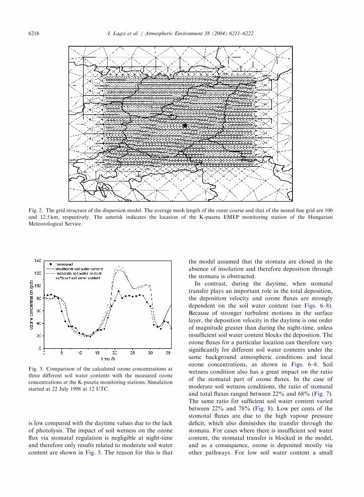
The simulated and measured ozone concentrations at

the K-puszta monitoring station of the Hungarian

Meteorological Service located about 80 km south of

Budapest (461580N, 191330E, 125m a.s.l.) are shown in

Fig. 3. The three simulated concentration data series

that correspond to the three assumed soil wetness states

are in accordance with the measured ones. According to

the results, the simulated ozone concentration practi-

cally does not depend on soil wetness conditions since

the greatest difference between the calculated data for

the three specified conditions is not higher than 5%.

These differences are higher during the daytime, but

lower in the night-time. In some cases the transport

model overestimated the measured ozone concentration.

No trivial source of these discrepancies has been found,

but these may be caused by uncertainties in the emisson

statistics, atmospheric data and also the local effects

around the monitoring station.

The simulated spatial distribution of ozone concen-

trations at 00 and 12UTC on 23 July 1998 are shown in

Fig. 4. Distribution of the deposition velocities and the

ozone fluxes at 00 UTC and for three different soil

wetness states (dry, moderately wet and wet) at 12UTC

on 23 July 1998 are presented in Figs. 5–8, respectively.

Additionally, for cases corresponding to moderately wet

and wet conditions, stomatal fluxes of ozone are also

plotted in Figs. 7 and 8, respectively.

Calculated deposition velocities of ozone over differ-

ent vegetation types were compared with observations

based on data from the literature (Table 3). The

modelled data are in good agreement with observed

ones.

The deposition velocity is low at night-time, because

stratification of the near surface layer is stable, and the

turbulence is weak. At this time, the ozone flux is mainly

controlled by the concentration of ozone, although this

ARTICLE IN PRESS

Fig. 3. Comparison of the calculated ozone concentrations at

three different soil water contents with the measured ozone

concentrations at the K-puszta monitoring stations. Simulation

started at 22 July 1998 at 12 UTC.

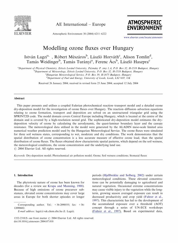
Fig. 2. The grid structure of the dispersion model. The average mesh length of the outer coarse and that of the nested fine grid are 100

and 12.5 km, respectively. The asterisk indicates the location of the K-puszta EMEP monitoring station of the Hungarian

Meteorological Service.

I. Lagzi et al. / Atmospheric Environment 38 (2004) 6211–62226216

is low compared with the daytime values due to the lack

of photolysis. The impact of soil wetness on the ozone

flux via stomatal regulation is negligible at night-time

and therefore only results related to moderate soil water

content are shown in Fig. 5. The reason for this is that

the model assumed that the stomata are closed in the

absence of insolation and therefore deposition through

the stomata is obstructed.

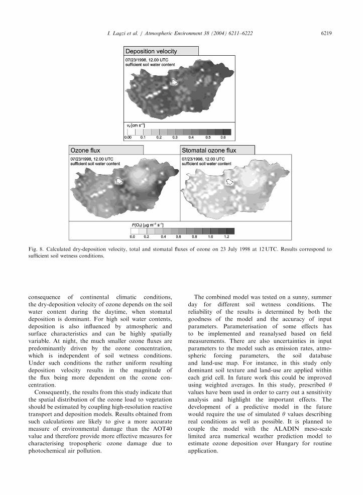
In contrast, during the daytime, when stomatal

transfer plays an important role in the total deposition,

the deposition velocity and ozone fluxes are strongly

dependent on the soil water content (see Figs. 6–8).

Because of stronger turbulent motions in the surface

layer, the deposition velocity in the daytime is one order

of magnitude greater than during the night-time, unless

insufficient soil water content blocks the deposition. The

ozone fluxes for a particular location can therefore vary

significantly for different soil water contents under the

same background atmospheric conditions and local

ozone concentrations, as shown in Figs. 6–8. Soil

wetness condition also has a great impact on the ratio

of the stomatal part of ozone fluxes. In the case of

moderate soil wetness conditions, the ratio of stomatal

and total fluxes ranged between 22% and 68% (Fig. 7).

The same ratio for sufficient soil water content varied

between 22% and 78% (Fig. 8). Low per cents of the

stomotal fluxes are due to the high vapour pressure

deficit, which also diminishes the transfer through the

stomata. For cases where there is insufficient soil water

content, the stomatal transfer is blocked in the model,

and as a consequence, ozone is deposited mostly via

other pathways. For low soil water content a small

ARTICLE IN PRESS

Fig. 4. Calculated ozone concentration on 23 July 1998 at 00 and 12UTC. Results correspond to moderate soil wetness conditions.

Fig. 5. Calculated dry-deposition velocity and flux of ozone on 23 July 1998 at 00UTC. Results correspond to moderate soil wetness

conditions.

Fig. 6. Calculated dry-deposition velocity and flux of ozone on 23 July 1998 at 12UTC. Results correspond to insufficient soil wetness

conditions.

I. Lagzi et al. / Atmospheric Environment 38 (2004) 6211–6222 6217

ARTICLE IN PRESS

Fig. 7. Calculated dry-deposition velocity, total and stomatal fluxes of ozone on 23 July 1998 at 12UTC. Results correspond to

moderate soil wetness conditions.

I. Lagzi et al. / Atmospheric Environment 38 (2004) 6211–62226218

dependency on local ozone concentrations is shown

during the daytime, where high ozone concentrations are

obtained in the region to the southeast of the city of

Budapest due to the formation of a plume from the city’s

emissions. Slightly higher ozone fluxes are predicted in

this region. In the city, the ozone concentration is much

lower due to the high local NO emission and the

reaction of NO with ozone to form NO2. In this region,

slightly lower ozone fluxes are observed. The differences

in ozone fluxes due to ozone concentrations are not,

however, as significant as those due to changes in soil

water content.

For higher soil wetness conditions a much greater

spatial variability in deposition velocity and ozone flux

than for low soil moisture conditions is seen. The soil

wetness stress for deposition is practically negligible for

wet soil conditions, and therefore ozone deposition is

mostly governed by atmospheric state variables (tem-

perature, relative humidity, etc.) and surface character-

istics (albedo, roughness length, etc.), which are

highly spatially variable. Again in this case, although

there is clearly some influence of local ozone concentra-

tions on ozone fluxes, other factors are also extremely

significant.

4. Conclusions

A chemical transport model and a dry-deposition

model were coupled for the purpose of simulating

ozone fluxes over Hungary. Flux calculations

without using a transport model are less precise,

because of the inaccurately known spatial distri-

bution of ozone concentrations estimated from

measurements at Hungarian monitoring stations. At

the same time, the spatial distribution of ozone

concentration is shown to be a less accurate

measure of effective ozone load than the spatial

distribution of ozone flux. This flux is determined by

the dry-deposition velocity of ozone, which has been

estimated for different surface types within the deposi-

tion model.

The main results from the simulation of the selected

scenario can be summarised as follows. In Hungary, as a

ARTICLE IN PRESS

Fig. 8. Calculated dry-deposition velocity, total and stomatal fluxes of ozone on 23 July 1998 at 12UTC. Results correspond to

sufficient soil wetness conditions.

I. Lagzi et al. / Atmospheric Environment 38 (2004) 6211–6222 6219

consequence of continental climatic conditions,

the dry-deposition velocity of ozone depends on the soil

water content during the daytime, when stomatal

deposition is dominant. For high soil water contents,

deposition is also influenced by atmospheric and

surface characteristics and can be highly spatially

variable. At night, the much smaller ozone fluxes are

predominantly driven by the ozone concentration,

which is independent of soil wetness conditions.

Under such conditions the rather uniform resulting

deposition velocity results in the magnitude of

the flux being more dependent on the ozone con-

centration.

Consequently, the results from this study indicate that

the spatial distribution of the ozone load to vegetation

should be estimated by coupling high-resolution reactive

transport and deposition models. Results obtained from

such calculations are likely to give a more accurate

measure of environmental damage than the AOT40

value and therefore provide more effective measures for

characterising tropospheric ozone damage due to

photochemical air pollution.

The combined model was tested on a sunny, summer

day for different soil wetness conditions. The

reliability of the results is determined by both the

goodness of the model and the accuracy of input

parameters. Parameterisation of some effects has

to be implemented and reanalysed based on field

measurements. There are also uncertainties in input

parameters to the model such as emission rates, atmo-

spheric forcing parameters, the soil database

and land-use map. For instance, in this study only

dominant soil texture and land-use are applied within

each grid cell. In future work this could be improved

using weighted averages. In this study, prescribed yvalues have been used in order to carry out a sensitivity

analysis and highlight the important effects. The

development of a predictive model in the future

would require the use of simulated y values describing

real conditions as well as possible. It is planned to

couple the model with the ALADIN meso-scale

limited area numerical weather prediction model to

estimate ozone deposition over Hungary for routine

application.

ARTICLE IN PRESS

Table 3

Comparison of observed and modelled dry-deposition velocities

Surface Summer observations Model calculation for Hungary Date: 23 July 1998

Mean Range Reference Condition Mean Range Condition

Grass 0.20 0.05–0.2 Padro (1996) Whole day 0.13 0.05–0.20 (1)

0.24 Meyers et al. (1998) Daytime 0.30 0.27–0.32 (2)

0.34 0.15–0.53 Zhang et al. (2002) Whole day 0.43 0.41–0.46 (3)

0.53 0.49–0.57 (4)

Agricultural

land

0.42 0.2–0.7 Baldocchi et al. (1987)—corn Daytime 0.15 0.05–0.30 (1)

0.32 Meyers et al. (1998)—corn Whole day 0.33 0.22–0.35 (2)

0.45 0.27–0.49 (3)

0.56 0.31–0.62 (4)

Orchard,

vineyard

0.3–0.5 Walton et al. (1997)––orchard Daytime 0.13 0.05–0.18 (1)

0.05–0.2 Night-time 0.21 0.20–0.22 (2)

0.33 0.15–0.51 Zhang et al. (2002)––vineyard Whole day 0.38 0.33–0.45 (3)

0.30 Zhang et al. (1996)––vineyard Whole day 0.54 0.46–0.65 (4)

Deciduous

forest

0.67 0.22–1.12 Zhang et al. (2002) Whole day 0.13 0.06–0.30 (1)

0.19–0.83 Meyers and Baldocchi (1988) Daytime 0.34 0.31–0.35 (2)

0.67 Zhang et al. (1996) Whole day 0.39 0.32–0.51 (3)

0.45 0.32–0.65 (4)

Mixed Forest 0.50 0.14–0.86 Zhang et al. (2002) Whole day 0.11 0.07–0.13 (1)

0.34 0.33–0.35 (2)

0.37 0.34–0.38 (3)

0.40 0.34–0.44 (4)

Lake 0.004–0.04 Wesely et al. (1981) 0.03 0.02–0.03 (1)

0.04 (2)–(3)–(4)

Conditions: (1) 00UTC; (2) 12UTC, insufficient soil water content; (3) 12UTC moderate soil water content; (4) 12UTC sufficient soil

water content.

I. Lagzi et al. / Atmospheric Environment 38 (2004) 6211–62226220

Acknowledgements

The authors acknowledge the support of OTKA grant

DO48673, T043770, F047242, OMFB grant 00585/2003

(IKTA5-137), UK-Hungarian cooperation grant GB50/

98 and the Bekesy Gyorgy Fellowship. The authors wish

to thank M. Berzins (University of Leeds), J. Gyorffy,

T. Perger (Eotvos Lorand University, Budapest),

A. Horanyi, G. Radnoti (Hungarian Meteorological

Service).

References

Acs, F., 2003. On the relationship between the spatial

variability of soil properties and transpiration. Ido+ jaras

107, 257–272.

Acs, F., Szasz, G., 2002. Characteristics of microscale

evapotranspiration: a comparative analysis. Theoretical

and Applied Climatology 73, 189–205.

Azzi, M., Johnson, G.J., Cope, M., 1992. An introduction to

the generic reaction set photochemical smog mechanism.

Proceedings of the 11th Clean Air Conference Fourth

Regional IUAPPA Conference, Brisbane, Australia, pp.

451–462.

Baldocchi, D.D., Hicks, B.B., Camara, P., 1987. A canopy

stomatal resistance model for gaseous deposition to

vegetated canopies. Atmospheric Environment 21,

91–101.

Berzins, M., Ware, J., 1995. Positive cell-centered finite volume

discretization methods for hyperbolic equations on irregular

meshes. Applied Numerical Mathematics 16, 417–438.

Berzins, M., Dew, P.M., Furzeland, R.M., 1989. Developing

software for time-dependent problems using the method of

lines and differential algebraic integrators. Applied Numer-

ical Mathematics 5, 375–390.

Brook, J.R., Zhang, L., Di-Giovanni, F., Padro, J., 1999.

Description and evaluation of a model of deposition

velocities for routine estimates of air pollutant dry deposi-

tion over North America. Part I: model development.

Atmospheric Environment 33, 5037–5051.

ARTICLE IN PRESSI. Lagzi et al. / Atmospheric Environment 38 (2004) 6211–6222 6221

De Santis, F., 1999. New directions: will a new European

vegetation ozone standard be fair to all European countries?

Atmospheric Environment 33, 3873–3874.

Emberson, L.D., Simpson, D., Tuovinen, J-P., Ashmore, M.R.

Cambridge, H.M., 2000a. Towards a model of ozone

deposition and stomatal uptake over Europe. EMEP

MSC-W Note 6/00.

Emberson, L.D., Ashmore, M.R., Cambridge, H.M., Simpson,

D., Touvinen, J.-P., 2000b. Modelling stomatal ozone flux

across Europe. Atmospheric Pollution 109, 403–413.

Fuhrer, J., Skarby, L., Ashmore, M.R., 1997. Critical levels for

ozone effects on vegetation in Europe. Environmental

Pollution 97, 91–106.

Grunhage, L., Haenel, H.-D., 1997. PLATIN (PLant-ATmo-

sphere INteraction) I: a model of plant-atmosphere inter-

action for estimating absorbed doses of gaseous air

pollutants. Environmental Pollution 98, 37–50.

Hart, G., Tomlin, A., Smith, J., Berzins, M., 1998. Multi-scale

atmospheric dispersion modelling by use of adaptive

gridding techniques. Environmental Monitoring and As-

sessment 52, 225–238.

Havasi, A., Zlatev, Z., 2002. Trends of Hungarian air pollution

levels on a long time-scale. Atmospheric Environment 36,

4145–4156.

Hicks, B.B., Baldocchi, D.D., Meyers, T.P., Hosker, R.P.,

Matt, D.R., 1987. A preliminary multiple resistance

routine for deriving dry deposition velocities from

measured quantities. Water, Air and Soil Pollution 36,

311–330.

Hjellbrekke, A-G., Solberg, S., 2002. Ozone measurments 2000.

EMEP/CCC-Report 5/2002.

Horanyi, A., Ihasz, I., Radnoti, G., 1996. ARPEGE/ALADIN:

a numerical Weather prediction model for Central-Europe

with the participation of the Hungarian Meteorological

Service. Issue Series Title: Ido+ jaras 100, 277–301.

Jarvis, P.G., 1976. The interpretation of the variations in leaf

water potential and stomatal conductance found in canopies

in the field. Philosophical Transactions of the Royal Society

of London Series B 273, 593–610.

Jonson, J.E., Sundet, J.K., Tarrason, L., 2001. Model calcula-

tions of present and future levels of ozone and ozone

precursors with a global and a regional model. Atmospheric

Environment 35, 525–537.

Karenlampi, L., Skarby, L. (Eds.), 1996. Critical levels for

ozone in Europe: Testing and finalizing the concepts.

UNECE Workshop Report. University of Kuopio, Depart-

ment of Ecology and Environmental Science, Kuopio,

Finland.

Klemm, O., Mangold, A., 2001. Ozone deposition at a forest

site in the Bavaria. Water, Air and Soil Pollution: Focus 1,

223–232.

Kramm, G., Dlugi, R., Dollard, G.J., Foken, Th., Molders, N.,

Muller, H., Seiler, W., Sievering, H., 1995. On the dry

deposition of ozone and reactive nitrogen species. Atmo-

spheric Environment 29, 3209–3231.

Krupa, S.V., Manning, W.J., 1988. Atmospheric ozone:

formation and effects on vegetation. Environmental Pollu-

tion 50, 101–137.

Lagzi, I., Tomlin, A.S., Turanyi, T., Haszpra, L., Meszaros, R.,

Berzins, M., 2001. The simulation of photochemical smog

episodes in Hungary and Central Europe using adaptive

gridding models. Lecture Notes in Computer Science 2074,

67–77.

Lagzi, I., Tomlin, A.S., Turanyi, T., Haszpra, L., Meszaros, R.,

Berzins, M., 2002. Modelling photochemical air pollution in

Hungary using an adaptive grid model. In: Sportisse, S.

(Ed.), Air Pollution Modelling and Simulation. Springer,

Berlin, pp. 264–273.

Lagzi, I., Karman, D., Turanyi, T., Tomlin, A.S., Haszpra, L.,

2004. Simulation of the dispersion of nuclear contamination

using an adaptive Eulerian grid model. Journal Environ-

mental Radioactivity 75, 59–82.

Meyers, T.P., Finkelstein, P., Clarke, J., Ellestad, T.G., Sims,

P.F., 1998. A multilayer model for inferring dry deposition

using standard meteorological measurements. Journal of

Geophysical Research 103, 22645–22661.

Mintz, Y., Walker, G.K., 1993. Global fields of soil moisture

and land surface evapotranspiration derived from observed

precipitation and surface air temperature. Journal of

Applied Meteorology 32, 1305–1334.

Padro, J., 1996. Summary of ozone dry deposition velocity

measurements and model estimates over vineyard, cotton,

grass and desciduous forest in summer. Atmospheric

Environment 30, 2363–2369.

Padro, J., den Hartog, G., Neumann, H.H., 1991. An

investigation of the ADOM dry deposition module using

summertime O3 measurements above a deciduous forest.

Atmospheric Environment 30, 339–345.

Padro, J., Zhang, L., Massman, W.J., 1998. An analysis of

mesurements and modelling of air-surface exchange of

NO–NO2–O3 over grass. Atmospheric Environment 32,

1167–1177.

Sofiev, M., Tuovinen, J-P., 2001. Factors determining the

robustness of AOT40 and other ozone exposure indices.

Atmospheric Environment 35, 3521–3528.

Tomlin, A., Berzins, M., Ware, J., Smith, J., Pilling, M.J., 1997.

On the use adaptive gridding methods for modelling

chemical transport from multi-scale sources. Atmospheric

Environment 31, 2945–2959.

Tuovinen, J-P., 2000. Assessing vegetation exposure to ozone:

properties of the AOT40 index and modifications by

deposition modelling. Environmental Pollution 109,

361–372.

Van Loon, M., 1996. Numerical methods in smog prediction.

Ph.D. Thesis, GWI Amsterdam.

Varallyay, Gy., Sz +ucs, L., Muranyi, A., Rajkai, K., Zilahy, P.,

1980. Map of soil factors determining the agro-ecological

potential of Hungary (1:100 000) II. Agrokemia es Talajtan

29, 35–76 (in Hungarian).

Walmsley, J.L., Wesely, M.L., 1996. Modification of coded

parameterizations of surface resistances to gaseous dry

deposition (Technical note). Atmospheric Environment 30,

1181–1188.

Walton, S., Gallagher, M.W., Choularton, T.W., Duyzer, J.,

1997. Ozone and NO2 exchange to fruit orchards. Atmo-

spheric Environment 31, 2767–2776.

Wesely, M.L., 1989. Parameterization of surface resistances to

gaseous dry deposition in regional-scale numerical models.

Atmospheric Environment 23, 1293–1304.

Wesely, M.L., Cook, D.R., Williams, R.M., 1981. Field

measurements of small ozone fluxes to snow, wet bare soil

and lake water. Boundary Layer Meteorology 20, 459–471.

ARTICLE IN PRESSI. Lagzi et al. / Atmospheric Environment 38 (2004) 6211–62226222

Zhang, L., Padro, J., Walmsley, J.L., 1996. A multi-layer model

vs. single-layer models and observed O3 dry

deposition velocities. Atmospheric Environment 25,

1689–1704.

Zhang, L., Moran, M.D., Brook, J.R., 2001. A comparison of

models to estimate in-canopy photosynthetically active

radiation and their influence on canopy stomatal resistance.

Atmospheric Environment 35, 4463–4470.

Zhang, L., Moran, M.D., Makar, P.A., Brook, R., Gong, S.,

2002. Modelling gaseous dry deposition in AURAMS: a

unified regional air-quality modelling system. Atmospheric

Environment 36, 537–560.