Intention-Aware Risk Estimation: Field Results

Stéphanie Lefèvre, Dizan Vasquez, Christian Laugier, Javier Ibañez-Guzmán

Abstract— This paper tackles the risk estimation problemfrom a new perspective: a framework is proposed for reasoningabout traffic situations and collision risk at a semantic level,while classic approaches typically reason at a trajectory level.Risk is assessed by estimating the intentions of drivers anddetecting conflicts between them, rather than by predictingthe future trajectories of the vehicles and detecting collisionsbetween them. More specifically, dangerous situations are iden-tified by comparing what drivers intend to do with what theyare expected to do according to the traffic rules. The reasoningis performed in a probabilistic manner, in order to take intoaccount sensor uncertainties and interpretation ambiguities.

This framework can in theory be applied to any type of trafficsituation; here we present its application to road intersections.The approach was validated with field trials using passenger ve-hicles equipped with Vehicle-to-Vehicle wireless communicationmodems. The results demonstrate that the algorithm is able todetect dangerous situations early and complies with real-timeconstraints.

I. INTRODUCTION

Active safety systems are increasingly present in commer-cial vehicles, as part of a global effort to make roads safer.The purpose of such systems is to avoid or mitigate accidentsthrough driver warnings or direct actions on the commands ofthe vehicles (braking, steering). At an algorithmic level, ac-tive safety functions rely on four processing steps: detect andtrack relevant entities in the environment (object assessmentstep), establish the relationship between these entities for abetter understanding of the situation (situation assessmentstep), estimate the level of danger of the current situation(risk assessment step), and decide on the best course of actionin order to promote safety (decision making step) [1].

The contribution of this paper concerns the second step.While classic approaches evaluate the risk of a traffic sit-uation by predicting the future trajectories of vehicles anddetecting collisions between them, we propose to reasonon risk at a semantic level. In the proposed framework,risk is assessed by estimating the intentions of drivers anddetecting conflicts between them. Traffic rules are explicitlyrepresented in our model, which makes it possible to estimateboth what drivers intend to do and what they are expected todo. Conflicts are then identified by comparing intentions andexpectations. This formulation of risk reflects the fact thatmost road accidents are caused by driver error [2], and hasthe advantage that it does not require to predict the futuretrajectories of vehicles.

S. Lefèvre, D. Vasquez, and C. Laugier are with Inria GrenobleRhône-Alpes, 655 av. de l’Europe - Montbonnot, 38334 Saint IsmierCedex, France, {stephanie.lefevre, alejandro-dizan.vasquez-govea, chris-tian.laugier}@inria.fr. J. Ibañez-Guzmán is with Renault S.A.S., 1 av. duGolf, 78288 Guyancourt, France, javier.ibanez-guzman@renault.com

The remainder of this paper is organized as follows.Section II reviews related work. Section III describes theproposed approach for risk assessment for general traffic sit-uations. Section IV describes the application of this generalframework to road intersections. Section V presents resultsobtained in field trials with passenger vehicles negotiating aT-shaped give-way intersection.

II. RELATED WORK

By far the most popular approaches to risk estimationare based on trajectory prediction [3]. The idea is to usea motion model to predict the possible future trajectories ofeach vehicle in the scene, and then to look for intersectionsbetween pairs of trajectories to detect future collisions.

Extensive research has been conducted on trajectory pre-diction. The most common solution is to rely on purelyphysical models (dynamic or kinematic) of the motion ofa vehicle [4], [5], [6], [7], [8], [9], however those cannotreason at a high level about the situation and thereforeare limited to short-term collision prediction. Long-termprediction can be improved by reasoning at a maneuverlevel instead of a purely physical level, and by taking intoaccount the constraints imposed by the road network onthe motion of vehicles. One strategy is to first identifythe maneuver intention of each driver and to then generatetrajectories corresponding to that maneuver intention onthe current road layout. For this purpose, Aoude et. al.[10] used a combination of Support Vector Machines andBayesian Filtering for maneuver intention estimation, andRapidly-exploring Random Trees for trajectory generation.As an alternative, Laugier et. al. [11] proposed to combineHidden Markov Models and Gaussian Processes. Anothersolution is to use Monte-Carlo simulation to explore thedifferent possible realizations of a maneuver by samplingon the input variables [12]. Other works propose integratedframeworks based on Markov State Space Models (MSSM)which explicitly represent the maneuver intention of driversand allow the prediction of future trajectories without theneed of a separate “maneuver intention estimation” step [13],[14], [15].

The main limitation of approaches based on trajectoryprediction is their high computational cost. For advancedmotion models, which take into account the local shape ofthe road layout and the dependencies between the motionof different vehicles, the cost of computing all the possiblefuture trajectories and the probability that they intersect isnot compatible with real-time safety applications. The classicsolution to reduce the complexity and the computation timeis to assume independence between vehicles. However this

leads to misinterpretations of traffic situations and to anoverestimation of the risk [16].

III. PROPOSED APPROACH FOR GENERAL TRAFFICSITUATIONS

To the best of our knowledge, only two motion modelshave been proposed in the literature which take into accountthe mutual dependencies between the vehicles [13], [14].Both are based on MSSMs and suffer from the limitationsmentioned in the previous section, i.e. the cost of predictingtrajectories using such models is prohibitive for real-timesafety applications. As an alternative we propose an approachto risk estimation which is also based on MSSMs but doesnot rely on trajectory prediction to estimate the risk of asituation.

A. Principle and examples

We propose to detect dangerous situations by comparingwhat drivers intend to do with what drivers are expected todo according to the traffic rules.

Example 1. Vehicle A is following vehicle B on thehighway, then vehicle B starts braking. In this situation thedriver of vehicle A is expected to either adapt its speedto the new speed of vehicle B, or to change lanes. If theintention of the driver does not match the expectation, e.g.if the driver intends to keep the same speed, the situationbecomes dangerous.

Example 2. Vehicle A is approaching a give-way inter-section, vehicle B is approaching the same intersection andhas the right-of-way. In this situation the driver of vehicleA is expected to yield to vehicle B if the time gap beforevehicle B reaches the intersection is too short for vehicle Ato execute its maneuver. If the intention of the driver does notmatch the expectation, e.g. if the driver intends to proceed inthe intersection while the time gap is too short, the situationbecomes dangerous.

This approach to risk assessment reflects the fact that mostroad accidents are caused by driver error [2], and matchesthe intuitive notion that “dangerous” situations are situationswhere drivers act differently from what is expected of them.

B. Implementation

As explained above, the proposed approach relies on theestimation of:

1) The maneuver that a driver intends to perform2) The maneuver that is expected of the driver

The former is already explicitly represented as a variablein the classic MSSM. The latter is implicitly encoded inthe classic MSSM, in the multi-vehicle dependencies. In theproposed MSSM, what is expected of the driver is madeexplicit by defining an additional variable. The differencesbetween the two models are illustrated graphically in Fig. 1and Fig. 2, and explained in more detail below.

In the classic MSSM (Fig. 1), the motion of a vehicle istypically modeled based on three layers of abstraction:

• The highest level corresponds to the maneuver per-formed by the vehicle (e.g. overtake, turn right at the

Fig. 1. Graphical representation of a classic MSSM. Bold arrows representmulti-vehicle dependencies, i.e. the influences of the other vehicles onvehicle n.

Fig. 2. Graphical representation of the proposed MSSM. Bold arrowsrepresent multi-vehicle dependencies, i.e. the influences of the other vehicleson vehicle n.

intersection). The variables at this level are discrete andhidden (not observable).We call I the conjunction of these variables. Int there-fore represents the maneuver being performed by vehi-cle n at time t. We call it I as “Intention”, since themaneuver performed by a vehicle reflects the intendedmaneuver of the driver.

• This level corresponds to the physical state of thevehicle (e.g. position, speed). The variables at this levelare hidden (not observable).We call Φ the conjunction of these variables. Φnt there-fore represents the physical state of vehicle n at timet.

• The lowest level corresponds to the measurementsavailable (e.g. measurement of the vehicle’s position).The variables at this level are observable. They oftencorrespond to a noisy version of a subset of the physicalvariables.We call Z the conjunction of these variables. Znttherefore represents the measurements of the state ofvehicle n at time t.

In this model, what a driver is expected to do is implicitlyencoded in the multi-vehicle dependencies: it is assumed thatthe current maneuver intention of the driver is dependenton the previous “situational context”, i.e. on the maneuverintention and physical state of the other vehicles (see boldarrows in Fig. 1). For example, it is assumed that a vehicledriving on the highway will - with a high probability -

slow down or change lanes if the vehicle in front startsbraking. Similarly, it is assumed that a driver approaching anintersection will - with a high probability - yield to vehicleswith right-of-way.

In the proposed MSSM (Fig. 2), what a driver is expectedto do is explicitly represented by the expected maneuverEnt . Ent is a conjunction of variables analogous to theintended maneuver Int : every variable in the conjunction Inthas an equivalent in the conjunction Ent . As can be seenin the graph, the expected maneuver Ent is derived fromthe previous situational context and has an influence on theintended maneuver Int .

In both the classic MSSM and the proposed MSSM, thedependencies between the vehicles are modeled by makingthe current intended maneuver Int dependent on the previous“situational context”. The difference is that the dependencyis not direct in the proposed MSSM: the expected maneuverEnt is inserted as an intermediate. The previous “situationalcontext” influences what the driver is expected to do, whichin turn influences what the driver intends to do.

C. Applications

Modeling explicitly what is expected of a vehicle attime t, as proposed above, creates new possibilities for theestimation of the risk of a situation. Instead of using theMSSM to predict the future trajectories of the vehicles, wepropose to use it to jointly infer what drivers currently intendto do (It) and what they are expected to do (Et). The risk of asituation is computed based on the probability that intentionand expectation do not match, given the measurements:

P ([Int 6= Ent ]|Z0:t) (1)

Based on Eq. 1, a variety of safety-oriented applications canbe derived.

1) Detection of hazardous vehicles: A “hazard probabil-ity” can be computed for every vehicle in the scene usingEq. 1. Subsequently, actions can be triggered depending onthe value of the risk. An example ADAS application wouldbe to warn all the drivers in the area when the risk is higherthan a predefined threshold, i.e. if:

∃n ∈ N : P ([Int 6= Ent ]|Z0:t) > λ (2)

The warning message could be adapted to the level of dan-ger, so that the driver is aware of the urgency of the situation.If autonomous braking is considered, the deceleration couldbe adapted to the risk value.

2) Risk of a specific maneuver: The risk of a specificmaneuver Int can be computed for a vehicle n:

P (

N⋃m=1

[Imt 6= Emt ]|Int Z0:t) (3)

This is an important feature for autonomous driving, butalso for ADAS. One application is to find the best escapemaneuver in a dangerous situation. Another one is to assistthe driver for tasks such as changing lanes on the highwayor negotiating an intersection by computing the risk of each

possible maneuver and informing the driver about how safeeach maneuver is.

3) Other applications: The proposed model can be usedto estimate the intended maneuver of a driver, or to predictfuture trajectories. These are useful features for numerousapplications which need to reason about traffic situations[17].

IV. APPLICATION TO ROAD INTERSECTIONS

The model presented in the previous section could intheory be applied to any traffic situations, by defining thevariables Int , Ent , Znt , and Φnt accordingly. This sectionpresents its application to unsignalized road intersections,i.e. intersections ruled by anything but traffic lights (stop,give-way, priority to the right). More specifically we addressaccidents caused by traffic sign violations. Driver error inthe lateral direction (such as hazardous lane changes) is notaddressed in this work.

The description of the algorithm follows the BayesianProgramming formalism [18]: first the variables are defined,then the proposed joint distribution, the parametric forms,and finally the calculation of risk. This algorithm has beendescribed in our previous publications [16], [19]; here theformulation has been modified to match the more generalrisk estimation framework presented in the previous section.

A. Variable definition

This section proposes definitions for the intended maneu-ver Int , the expected maneuver Ent , the physical state Φnt , andthe measurements Znt , in the context of road intersections.

1) Intended maneuver : As was mentioned above, thefocus of this work is on errors in the longitudinal executionof the maneuver. Since we want to be able to reason on thelateral motion and on the longitudinal motion separately, wemake a distinction between the lateral and longitudinal com-ponents of a maneuver in our specification of the intendedmaneuver Int .Lateral component: For the lateral component we exploit thefact that intersections are highly structured areas where thelateral motion of vehicles is constrained by the geometry andthe topology of the intersection. It is assumed that a digitalmap of the road network is available. From this digital mapwe extract a set of “courses”, where a course is defined foreach authorized maneuver at the intersection as the typicalpath that is followed by a vehicle when executing thatparticular maneuver. The concept of a course is illustrated inFig. 3. The variable representing the lateral component of amaneuver is defined as:

• Icnt ∈ {ci}i=1:NC: the driver’s intended lateral motion,

which will also be called the driver’s intended course inthe context of road intersections. It corresponds to thecourse followed by vehicle n at time t. {ci}i=1:NC

isthe set of possible courses at the intersection, extractedfrom the digital map.

Longitudinal component: For the longitudinal component weexploit the fact that intersections are highly structured areaswhere the longitudinal motion of vehicles is constrained by

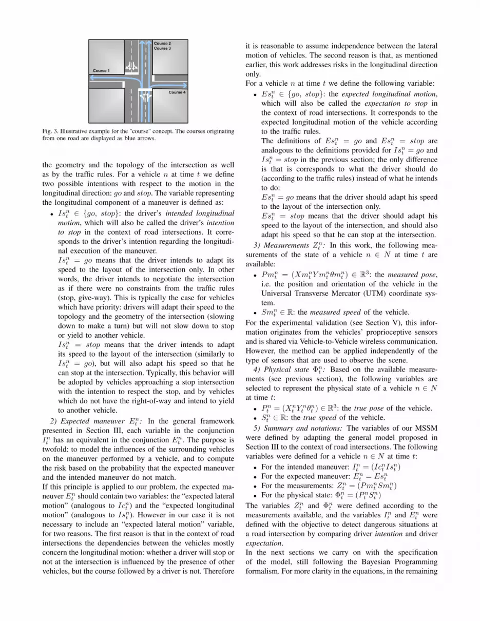
Fig. 3. Illustrative example for the "course" concept. The courses originatingfrom one road are displayed as blue arrows.

the geometry and the topology of the intersection as wellas by the traffic rules. For a vehicle n at time t we definetwo possible intentions with respect to the motion in thelongitudinal direction: go and stop. The variable representingthe longitudinal component of a maneuver is defined as:

• Isnt ∈ {go, stop}: the driver’s intended longitudinalmotion, which will also be called the driver’s intentionto stop in the context of road intersections. It corre-sponds to the driver’s intention regarding the longitudi-nal execution of the maneuver.Isnt = go means that the driver intends to adapt itsspeed to the layout of the intersection only. In otherwords, the driver intends to negotiate the intersectionas if there were no constraints from the traffic rules(stop, give-way). This is typically the case for vehicleswhich have priority: drivers will adapt their speed to thetopology and the geometry of the intersection (slowingdown to make a turn) but will not slow down to stopor yield to another vehicle.Isnt = stop means that the driver intends to adaptits speed to the layout of the intersection (similarly toIsnt = go), but will also adapt his speed so that hecan stop at the intersection. Typically, this behavior willbe adopted by vehicles approaching a stop intersectionwith the intention to respect the stop, and by vehicleswhich do not have the right-of-way and intend to yieldto another vehicle.

2) Expected maneuver Ent : In the general frameworkpresented in Section III, each variable in the conjunctionInt has an equivalent in the conjunction Ent . The purpose istwofold: to model the influences of the surrounding vehicleson the maneuver performed by a vehicle, and to computethe risk based on the probability that the expected maneuverand the intended maneuver do not match.If this principle is applied to our problem, the expected ma-neuver Ent should contain two variables: the “expected lateralmotion” (analogous to Icnt ) and the “expected longitudinalmotion” (analogous to Isnt ). However in our case it is notnecessary to include an “expected lateral motion” variable,for two reasons. The first reason is that in the context of roadintersections the dependencies between the vehicles mostlyconcern the longitudinal motion: whether a driver will stop ornot at the intersection is influenced by the presence of othervehicles, but the course followed by a driver is not. Therefore

it is reasonable to assume independence between the lateralmotion of vehicles. The second reason is that, as mentionedearlier, this work addresses risks in the longitudinal directiononly.For a vehicle n at time t we define the following variable:

• Esnt ∈ {go, stop}: the expected longitudinal motion,which will also be called the expectation to stop inthe context of road intersections. It corresponds to theexpected longitudinal motion of the vehicle accordingto the traffic rules.The definitions of Esnt = go and Esnt = stop areanalogous to the definitions provided for Isnt = go andIsnt = stop in the previous section; the only differenceis that is corresponds to what the driver should do(according to the traffic rules) instead of what he intendsto do:Esnt = go means that the driver should adapt his speedto the layout of the intersection only.Esnt = stop means that the driver should adapt hisspeed to the layout of the intersection, and should alsoadapt his speed so that he can stop at the intersection.

3) Measurements Znt : In this work, the following mea-surements of the state of a vehicle n ∈ N at time t areavailable:

• Pmnt = (Xmn

t Y mnt θm

nt ) ∈ R3: the measured pose,

i.e. the position and orientation of the vehicle in theUniversal Transverse Mercator (UTM) coordinate sys-tem.

• Smnt ∈ R: the measured speed of the vehicle.

For the experimental validation (see Section V), this infor-mation originates from the vehicles’ proprioceptive sensorsand is shared via Vehicle-to-Vehicle wireless communication.However, the method can be applied independently of thetype of sensors that are used to observe the scene.

4) Physical state Φnt : Based on the available measure-ments (see previous section), the following variables areselected to represent the physical state of a vehicle n ∈ Nat time t:

• Pnt = (Xnt Y

nt θ

nt ) ∈ R3: the true pose of the vehicle.

• Snt ∈ R: the true speed of the vehicle.5) Summary and notations: The variables of our MSSM

were defined by adapting the general model proposed inSection III to the context of road intersections. The followingvariables were defined for a vehicle n ∈ N at time t:

• For the intended maneuver: Int = (Icnt Isnt )

• For the expected maneuver: Ent = Esnt• For the measurements: Znt = (Pmn

t Smnt )

• For the physical state: Φnt = (Pnt Snt )

The variables Znt and Φnt were defined according to themeasurements available, and the variables Int and Ent weredefined with the objective to detect dangerous situations ata road intersection by comparing driver intention and driverexpectation.In the next sections we carry on with the specificationof the model, still following the Bayesian Programmingformalism. For more clarity in the equations, in the remaining

of this article a bold symbol will be used to represent theconjunction of variables for all the vehicles in the scene. Forexample, for a variable X:

X , (X1...XN ) (4)

with Xn the variable associated with vehicle n.

B. Joint distributionFor the general model proposed in Fig. 2, the joint

distribution over all the vehicles is as follows:

P (E0:TI0:TΦ0:TZ0:T) = P (E0I0Φ0Z0)

×T∏t=1

×N∏n=1

[P (Ent |It−1Φt−1)× P (Int |Φnt−1Int−1E

nt )

×P (Φnt |Φnt−1Int−1I

nt )× P (Znt |Φnt )] (5)

In this section we adapt this general model to road inter-section situations, with the variables defined in the previoussection. We start by making the following classic indepen-dence assumptions:

For the intended maneuver: The current intended lateralmotion and intended longitudinal motion are conditionallyindependent given (Φnt−1I

nt−1E

nt ). Therefore the following

simplification is obtained:

P (Int |Φnt−1Int−1E

nt ) = P (Icnt |Φnt−1I

nt−1E

nt )×P (Isnt |Φnt−1I

nt−1E

nt )

(6)For the physical state: The current pose and current speed

are conditionally independent given (Φnt−1Int−1I

nt ). There-

fore the following simplification is obtained:

P (Φnt |Φnt−1Int−1I

nt ) = P (Pnt |Φnt−1I

nt−1I

nt )×P (Snt |Φnt−1I

nt−1I

nt )(7)

For the measurements: A classic sensor model is used, i.e.the measurements are conditionally independent given thephysical quantities they are associated with. Therefore thefollowing simplification is obtained:

P (Znt |Φnt ) = P (Pmnt |Pnt )× P (Smn

t |Snt ) (8)

After applying these independence assumptions, and takinginto account that Ent = Esnt , the joint distribution (Eq. 5)becomes:

P (E0:TI0:TΦ0:TZ0:T) = P (E0I0Φ0Z0)

×T∏t=1

×N∏n=1

[P (Esnt |It−1Φt−1)

× P (Icnt |Φnt−1Int−1Es

nt )× P (Isnt |Φnt−1I

nt−1Es

nt )

× P (Pnt |Φnt−1Int−1I

nt )× P (Snt |Φnt−1I

nt−1I

nt )

×P (Pmnt |Pnt )× P (Smn

t |Snt )] (9)

C. Parametric forms

In this section the parametric forms of the conditionalprobability terms in Eq. 9 are described, along with thehypotheses they build on.

1) Expected longitudinal motion Esnt : The expected lon-gitudinal motion of a vehicle is derived from the previousintended course, pose and speed of all the vehicles in thescene:

P (Esnt |It−1Φt−1) = P (Esnt |Ict−1Pt−1St−1) (10)

What is expected of vehicles on the road is regulated bytraffic rules, but a lot is left to the judgment of drivers. Ifwe take as an example give-way intersections in France, therules specify that the driver which does not have the right-of-way must “yield to vehicles driving on the other road(s) andmake sure there is no danger before entering the intersection”[20]. There exists no formula to calculate whether it is legalor not for a driver to enter an intersection at time t in aspecific context. Instead, our expectation model is based ontypical driver behavior, i.e. on a statistical analysis of whatdrivers consider to be acceptable. The necessity for a vehicleto stop given the context is derived using probabilistic gapacceptance models [21], [22]:

P ([Esnt = stop]|[Ict−1 = ct−1][Pt−1 = pt−1][St−1 = st−1])

= f(ct−1, pt−1, st−1) (11)

with ct−1 the conjunction of courses for the N vehiclesin the scene, pt−1 the conjunction of positions for the Nvehicles in the scene, st−1 the conjunction of speeds for theN vehicles in the scene, and f a function which computes theprobability that the gap available for vehicle n to execute itsmaneuver is sufficient given the previous situational context(ct−1, pt−1, st−1). For a vehicle n heading towards a give-way intersection, the calculation is detailed below:

i. Project forward (or backward) the position of vehiclen until the time tn when it reaches the intersection,using the vehicle’s previous state (cnt−1, p

nt−1, s

nt−1)

and a constant speed model.ii. Let VROW be the set of vehicles whose maneuvers

have the right-of-way w.r.t. the maneuver of vehiclen. For each vehicle m ∈ VROW project forward (orbackward) the position of vehicle m until the time tm

when it reaches the intersection, using the vehicle’sprevious state (cmt−1, p

mt−1, s

mt−1) and a constant speed

model.iii. Find the vehicle k ∈ VROW which is the most likely

to cause vehicle n to stop, by finding the smallestpositive time gap available for vehicle n to executeits maneuver:k = arg min

m∈VROW

(tm − tn), for tm − tn ≥ 0

gmin = tk − tn(12)

iv. The necessity for vehicle n to stop at the intersectionis calculated as the probability that the gap gmin is notsufficient, using a probabilistic gap acceptance model([21] for merging cases, [22] for left turn across pathcases).

For a vehicle approaching a stop intersection the calculationis similar, except the probability that the vehicle is expected

to stop is set to 1 until it reaches the intersection (i.e.P ([Esnt = stop]|Ict−1Pt−1St−1) = 1), and after that pointthe last two steps of the calculation above are used (i.e. steps3 and 4).This context-aware reasoning about the necessity for a vehi-cle to stop at the intersection will allow us to detect vehiclesrunning stop signs, or vehicles entering an intersection whenthey should have waited for another vehicle to pass.

2) Intended longitudinal motion Isnt : A number of differ-ent strategies could be applied for the intended longitudinalmotion model, to model drivers’ habits in terms of com-pliance with traffic rules. In this work, the evolution modelis based on the comparison between the previous intentionIsnt−1 and the current expectation Esnt :

P (Isnt |Φnt−1Int−1Es

nt ) = P (Isnt |Isnt−1Es

nt ) (13)

If the driver’s intention at time t − 1 coincides with whatis currently expected of him, it is assumed that the driverwill comply with a probability Pcomply. Otherwise a uniformprior (0.5) is assumed:

Isnt−1 Esnt P ([Isnt = go]|Isnt−1Esnt )

go go Pcomplygo stop 0.5

stop go 0.5

stop stop 1.0− Pcomply

The probability Pcomply is set to Pcomply = 0.9 to reflect ourassumption that chances are high that the driver will comply,but ideally it should be learned from data.

3) Intended lateral motion Icnt : In the general case of avehicle driving from point A to point B on the road network,the lateral motion will change with time as one maneuver isperformed after another. In this work the focus is on roadintersections, and the possible lateral motions were defined asa set of possible courses. Courses cover the entire maneuverat the intersection (approaching phase + execution inside theintersection + exit phase), and there is no reason to believethat a driver will change his mind about the course he wantsto follow. For this reason, it is assumed that the probabilityof a course at time t is dependent on the previous intendedcourse only (Eq. 14) and that drivers keep the same intentionbetween two timesteps with probability Psame, all the othercourses being equally probable (Eq. 15).

P (Isnt |Φnt−1Int−1Es

nt ) = P (Icnt |Icnt−1) (14)

P ([Icnt = cnt ]|[Icnt−1 = cnt−1]) =

{Psame if cnt = cnt−11.0−PsameNC−1

otherwise

(15)The value of Psame was set manually to Psame = 0.9 to

indicate that drivers rarely change their intended course, butshould ideally be learned from data.

4) Pose Pnt : It is assumed that a vehicle performinga maneuver will follow the course corresponding to thatmaneuver. The evolution of the pose of a vehicle is computed

from its previous pose, previous speed, and current intendedcourse:

P (Pnt |Φnt−1Int ) = P (Pnt |Pnt−1S

nt−1Ic

nt ) (16)

The likelihood of a pose is defined as a trivariate normaldistribution with no correlation between x, y and θ:

P (Pnt |[Pnt−1 = pnt−1][Snt−1 = snt−1][Icnt = cnt−1])

= N (µxyθ(pnt−1, s

nt−1, c

nt−1), σxyθ) (17)

where µxyθ(pnt−1, snt−1, c

nt−1) is a function which computes

the mean pose (µx, µy, µθ), and σxyθ = (σx, σy, σθ) is thestandard deviation.The mean pose of the vehicle is computed from the previouspose, the previous speed, and the current maneuver intentionas the average between two poses: the first one is obtainedthrough a constant velocity model, the second one is obtainedby projecting the first one orthogonally on the exemplar path.This average provides a compromise between the currentpose of the vehicle and the “ideal” pose that the vehiclewould have if following the exemplar path.

5) Speed Snt : It is assumed that drivers adapt their speedto their intentions and to the geometry of the road. The evo-lution of the speed of a vehicle is computed from its previousspeed, previous pose, and current intended maneuver:

P (Snt |Φnt−1Int ) = P (Snt |Snt−1P

nt−1Ic

nt Is

nt ) (18)

The distribution on Snt is assumed normal and defined as:

P (Snt |[Snt−1 = snt−1][Pnt−1 = pnt−1][Icnt = cnt ][Isnt = isnt ])

= N (µs(snt−1, p

nt−1, c

nt , is

nt ), σs(s

nt−1, p

nt−1, c

nt , is

nt )) (19)

where µs(snt−1, pnt−1, c

nt , is

nt ) is a function which computes

the mean speed and σs(snt−1, p

nt−1, c

nt , is

nt ) is a function

which computes the standard deviation.The mean speed is computed as a function of the previousspeed, the previous pose, the current course intention, andthe current intention to stop, using a set of typical speedprofiles. These speed profiles are created based on genericspeed profiles of vehicles negotiating intersections found inthe literature [23]. These generic speed profiles are automat-ically modified in our algorithm to match the speed limitand the geometry of the intersection of interest (e.g. thespeed is made dependent on the curvature of the course).Moreover the calculation of the mean speed accounts forsome variations in the driving styles, by taking into accountthe previous speed of the vehicle snt−1. The predicted speedprofile will therefore adapt to “sporty” drivers as well as tomore “relaxed” drivers.

6) Measured pose Pmnt : A classic sensor model is as-

sumed, with a trivariate normal distribution centered on thetrue state and with no correlation between x, y and θ:

P (Pmnt |[Pnt = pnt ]) = N (pnt , σxyθ) (20)

7) Measured speed Smnt : A classic sensor model is

assumed, with a normal distribution centered on the truestate:

P (Smnt |[Snt = snt ]) = N (snt , σs) (21)

8) Summary: Throughout this section a number of in-dependence assumptions were made. As a result the jointdistribution in Eq. 9 becomes:

P (E0:TI0:TΦ0:TZ0:T) = P (E0I0Φ0Z0)

×T∏t=1

×N∏n=1

[P (Esnt |Ict−1Pt−1St−1)

× P (Icnt |Icnt−1)× P (Isnt |Isnt−1Esnt )

× P (Pnt |Pnt−1Snt−1Ic

nt )× P (Snt |Snt−1P

nt−1Ic

nt Is

nt )

×P (Pmnt |Pnt )× P (Smn

t |Snt )] (22)

D. Bayesian risk estimation

The equation for risk estimation is given in Eq. 1 forgeneral traffic situations. When applied to our problem, theprinciple of comparing intention and expectation leads tocomputing the risk based on the probability that a driver doesnot intend to stop at the intersection while he is expected to:

P ([Isnt = go][Esnt = stop]|Pm0:tSm0:t) (23)

Exact inference on such a non-linear non-Gaussian modelis not tractable. Here, approximate inference is performedusing the classic bootstrap filter [24]. For two vehicles, wefound that a good compromise between computation timeand quality of the estimation was achieved for a number ofparticles Nparticles = 400.

V. FIELD TRIALS

A. Evaluation strategy

Evaluating the performance of risk assessment algorithmsis not straightforward: the ground truth of the risk of asituation is not available, therefore the evaluation cannot beconducted on the output of the algorithm directly. Instead itis generally conducted at the “application” level by applyinga threshold on the risk value to separate dangerous and non-dangerous situations. The algorithm is then evaluated basedon:

1. The rate of false alarms, i.e. non-dangerous situationsclassified as dangerous by the algorithm

2. The rate of missed detections, i.e. dangerous situationsclassified as non-dangerous by the algorithm

3. The collision prediction horizon, i.e. how early thealgorithm classifies the situation as dangerous

Throughout this section, dangerous and non-dangerous sit-uations are classified using the “hazard probability” crite-rion introduced in Section III-C.1. The idea is to computea “hazard probability” for every vehicle in the scene bycomparing the driver’s intention Isnt with the expectation

Fig. 4. Test scenarios for the field trials. For each scenario the maneuverof the Other Vehicle (OV) is shown in dotted red and the maneuver of thePriority Vehicle (PV) is shown in plain green.

Esnt . Subsequently a situation is classified as dangerous ifthe hazard probability is higher than a threshold for at leastone vehicle, i.e. iff:

∃n ∈ N : P ([Isnt = go][Esnt = stop]|Pm0:tSm0:t) > λ (24)

The threshold λ is set with the double objective to detectdangerous situations as early as possible and to avoid falsealarms in non-dangerous situations. After a recall and pre-cision analysis, λ = 0.3 was found to be the optimal valueand was used in all the experiments.

B. Experimental setup

Two passenger vehicles were equipped with off-the-shelfVehicle-to-Vehicle communication modems (802.11p) andshared their pose and speed information at a rate of 10 Hz.In each vehicle the pose and speed information was obtainedvia a GPS + IMU unit with a precision of σ = 2mfor the position. In its current non-optimized state the riskestimation algorithm runs at 10 Hz on a dedicated dual core2.26 GHz processor PC. The test vehicles were not equippedwith autonomous emergency braking functions. Instead, anauditory and a visual warning were triggered whenever thealgorithm detected a dangerous situation.

C. Scenarios

Experiments were conducted at a T-shaped give-way in-tersection for two collision scenarios. The scenarios areillustrated in Fig. 4. All of them involve a Priority Vehi-cle (PV) driving on the main road and an Other Vehicle(OV) performing a dangerous maneuver. In these scenarios,emergency braking is the only way to avoid an accident,therefore we expect the application to issue a warning asearly as possible.

Non-dangerous tests were also run, with the same config-urations as in Fig. 4 but this time following the traffic laws.

In total 90 dangerous and 20 non-dangerous tests wererun. We alternated between 6 different drivers both for thePV and the OV. In order to generate some diversity in thescenario instances, the drivers of the OV were not givenprecise instructions about the execution of the maneuvers;they were told to execute the maneuver in a manner thatthey felt was dangerous or non-dangerous. Out of the 90dangerous trials, 60 were performed with the warning systemrunning on the PV, and 30 running on the OV.

Fig. 5. Dangerous situation detected during the field trials (view from inside the Priority Vehicle).

D. Results

In the 20 non-dangerous tests there was no false alarm,i.e. no warning was ever triggered by the system.

For every of the 90 dangerous tests, the system was ableto issue a warning early enough that the driver avoided thecollision by braking. Fig. 5 shows a sample dangerous leftturn across path scenario during which we recorded the viewfrom inside the PV. The danger is detected as soon as the OVstarts to execute the left turn. The driver of the PV receivesa warning indicating that a dangerous situation was detectedand that the danger comes from a vehicle on the left side.

Since we did not create real collisions, we could notperform a statistical analysis about the collision predictionhorizon like was done in [16], [19]. However, the field trialsdemonstrated that our approach can operate with success inreal-life situations where passenger vehicles share data via aVehicle-to-Vehicle wireless link.

VI. CONCLUSIONS

In this paper a probabilistic framework was proposedto reason about the motion of vehicles and the associatedrisk in general traffic situations. The intentions of driversare explicitly modeled, as well as what the traffic rulesexpect of drivers in the current situation. Risk is thencomputed as the probability that intentions and expectationsdo not match, given the available observations. As opposedto classic approaches relying on trajectory prediction, theproposed approach reasons about risk at a semantic level.As a result it can run in real-time without having to assumeindependence between vehicles. Tests were conducted withpassenger vehicles equipped with off-the-shelf Vehicle-to-Vehicle communication modems at a T-shaped give-wayintersection. The results show that the algorithm is able todetect dangerous situations in real-time for different types ofcollision scenarios.

REFERENCES

[1] D. Hall and J. Llinas, “An introduction to multisensor data fusion,”Proceedings of the IEEE, vol. 85, no. 1, pp. 6–23, 1997.

[2] TRACE project, “Accident causation and pre-accidental driving situa-tions - In-depth accident causation analysis,” Deliverable D2.2, 2008.

[3] S. Lefèvre et al., “A survey on motion prediction and risk assessmentfor intelligent vehicles,” Robomech Journal, vol. 1, no. 1, 2014.

[4] S. Ammoun and F. Nashashibi, “Real time trajectory prediction forcollision risk estimation between vehicles,” in Proc. IEEE IntelligentComputer Communication and Processing, 2009, pp. 417–422.

[5] M. Brännström et al., “Model-based threat assessment for avoidingarbitrary vehicle collisions,” IEEE Transactions on Intelligent Trans-portation Systems, vol. 11, no. 3, pp. 658–669, 2010.

[6] T. Batz et al., “Recognition of dangerous situations within a coopera-tive group of vehicles,” in Proc. IEEE Intelligent Vehicles Symposium,2009, pp. 907–912.

[7] A. Eidehall and L. Petersson, “Statistical threat assessment for generalroad scenes using Monte Carlo sampling,” IEEE Transactions onIntelligent Transportation Systems, vol. 9, no. 1, pp. 137–147, 2008.

[8] J. Hillenbrand et al., “A multilevel collision mitigation approach:situation assessment, decision making, and performance tradeoffs,”IEEE Transactions on Intelligent Transportation Systems, vol. 7, no. 4,pp. 528–540, 2006.

[9] A. Polychronopoulos et al., “Sensor fusion for predicting vehicles’path for collision avoidance systems,” IEEE Transactions on IntelligentTransportation Systems, vol. 8, no. 3, pp. 549–562, 2007.

[10] G. S. Aoude et al., “Threat assessment design for driver assistancesystem at intersections,” in Proc. IEEE Intelligent TransportationSystems Conference, 2010, pp. 25–30.

[11] C. Laugier et al., “Probabilistic analysis of dynamic scenes andcollision risks assessment to improve driving safety,” IEEE IntelligentTransportation Systems Magazine, vol. 3, no. 4, pp. 4–19, 2011.

[12] M. Althoff and A. Mergel, “Comparison of Markov chain ab-straction and Monte Carlo simulation for the safety assessment ofautonomous cars,” IEEE Transactions on Intelligent TransportationSystems, vol. 12, no. 4, pp. 1237–1247, 2011.

[13] G. Agamennoni et al., “Estimation of multivehicle dynamics byconsidering contextual information,” IEEE Transactions on Robotics,vol. 28, no. 4, pp. 855–870, 2012.

[14] T. Gindele et al., “A probabilistic model for estimating driver behav-iors and vehicle trajectories in traffic environments,” in Proc. IEEEIntelligent Transportation Systems Conference, 2010, pp. 1625–1631.

[15] N. Oliver and A. P. Pentland, “Graphical models for driver behaviorrecognition in a SmartCar,” in Proc. IEEE Intelligent Vehicles Sympo-sium, 2000, pp. 7–12.

[16] S. Lefèvre et al., “Risk assessment at road intersections: comparingintention and expectation,” in Proc. IEEE Intelligent Vehicles Sympo-sium, 2012, pp. 165–171.

[17] L. Fletcher et al., “The MIT-Cornell collision and why it happened,”Journal of Field Robotics, vol. 25, pp. 775–807, 2008.

[18] O. Lebeltel et al., “Bayesian robot programming,” Autonomous Robots,vol. 16, no. 1, pp. 49–79, 2004.

[19] S. Lefèvre et al., “Evaluating risk at road intersections by detectingconflicting intentions,” in Proc. IEEE/RSJ International Conference onIntelligent Robots and Systems, 2012, pp. 4841–4846.

[20] “Code de la route français - Article R415-7,” available athttp://www.legifrance.gouv.fr.

[21] A. Spek et al., “Intersection approach speed and accident probability,”Transportation Research Part F: Traffic Psychology and Behaviour,vol. 9, no. 2, pp. 155–171, 2006.

[22] D. R. Ragland et al., “Gap acceptance for vehicles turning leftacross on-coming traffic: implications for intersection decision supportdesign,” in Proc. Transportation Research Board Annual Meeting,2006.

[23] H. Berndt et al., “Driver braking behavior during intersection ap-proaches and implications for warning strategies for driver assistantsystems,” in Proc. IEEE Intelligent Vehicles Symposium, 2007, pp.245–251.

[24] M. S. Arulampalam et al., “A tutorial on particle filters for onlinenonlinear/non-Gaussian Bayesian tracking,” IEEE Transactions onSignal Processing, vol. 50, no. 2, pp. 174–188, 2002.