Energy-Aware Process Design Optimization

Cinzia Cappiello, Pierluigi Plebani, and Monica VitaliDipartimento di Elettronica, Informazione e Bioingegneria - Politecnico di Milano

Piazza Leonardo da Vinci, 32 - 20133 Milan, ItalyEmail: cinzia.cappiello@polimi.it, pierluigi.plebani@polimi.it, vitali@elet.polimi.it

Abstract—Cloud computing has a big impact on the envi-ronment since the energy consumption and the resulting CO2emissions of data centers can be compared to the worldwideairlines traffic. Many researchers are addressing such issueby proposing methods and techniques to increase data centerenergy efficiency. Focusing at the application level, this paperproposes a method to support the process design by optimizingthe configuration and deployment. In particular, measuring andmonitoring suitable metrics, the presented approach provides asupport to the designer to select the way in which it is possible tomodify the process deployment in order to continuously guaranteegood performance and energy efficiency. The process adaptationcan be required when inefficiencies occur or when, although thesystem is efficient, there is still room for improvements.

I. INTRODUCTION

Nowadays, researchers are more and more analyzing theevolution and diffusion of cloud computing from a perspectiveon sustainability. Assessments of the environmental impact ofcloud computing reveal that data centers consume an extremelyhigh amount of electricity [1]. Many contributions show thatthe reduction of CO2 emissions, and energy consumption canbe achieved by considering several initiatives such as thereduction of the cooling power consumption, the utilization ofgreen energy sources, server consolidation and virtualization,and the utilization of greener machines. In the proposedapproaches, less attention has been paid to the analysis ofthe impact of the design and deployment of the runningapplications on energy efficiency.

Considering this application viewpoint, in this paper wepropose an approach for the optimization of the applicationdesign and deployment. The optimization is driven by threemain factors: energy consumption, CO2 emissions, and thesatisfaction of performance requirements measured by suitablemetrics. The idea is to follow a process design life-cyclewhere firstly, a business process (BP), i.e., a set of tasks, isdesigned and deployed on the basis of the characteristics ofthe system and of the designer expertise. Then, the systemcontinuously monitors the application in order to evaluateif the requirements are satisfied or if there is anyway roomfor improving the considered metrics. If changes are needed,the designer should enact appropriate adaptation actions, thatwill take place in the next execution of the BP and that areable to address the discovered inefficiencies, by modifyingthe workload distribution between different versions of theconsidered BP. The approach described in this paper aims tosupport the designer in the interpretation of the monitoringresults and in the selection of the adaptation action.

The paper is organized as follows. Section II discussesprevious contributions and highlights the innovative aspects of

the presented approach. Section III provides a general overviewof the approach that is formalized in the following sections:Section IV focuses on the process design and deploymentphases, Section V introduces the relevant metrics, Section VIdescribes the method that supports the designer in the selectionof the adaptation action able to optimize the process in termsof performance and energy efficiency. Finally, Section VIIvalidates the approach with an example and Section VIIIoutlines some possible future work.

II. RELATED WORKS

Energy efficiency and the control of CO2 emissions are aliving matter and, in the recent years, many researcher haveaddressed these aspects at very different granularity levels. Themain issue when dealing with energy efficiency and CO2 emis-sions consists in finding a direct or indirect way to measurethem. Moreover, the improvement in energy efficiency andthe CO2 emissions reduction cannot overlook the impact overperformance. A tradeoff between greenness and performancehas to be handled in order to respect functional requirementsof the provided services. Metrics for describing these twoaspects have been formalized in [2] and in [3]. In the formerwork, the well known Key Performance Indicators (KPIs) forevaluating Quality of Service (QoS) are integrated with a set ofenergy related metrics called Key Ecological Indicators (KEIs).The latter work introduces the concept of Green PerformanceIndicators (GPIs), with a role similar to the KEIs. In [4],authors put lights on the importance of considering also howthe available resources are used in the delivery of the service,introducing usage centric metrics to this extent. This concept isdeveloped also in [5], where usage centric metrics are definedat the server and the virtual machine level.

Measuring energy is not an easy task, especially when realtime data are required and when energy has to be measuredfor each single server separately. Several approaches considerCPU as the principal contributor to power usage in a serverand propose models for computing energy starting from theamount of CPU used on the server [6] [7] [8] [9] [10]. Thesemodels compute power usage using a linear relation betweenCPU usage and power consumption. Parameters of the modelare the power consumption values for the server when idleand when at the peak load. The only variable of the modelis the CPU load. It has been demonstrated that even a linearapproximation of this model is effective in estimating the realpower consumption [11]. An interesting aspect is that even inidle state a server consumes more than the 60% of its peak loadpower. This is why an optimization, even at the applicationlevel can significantly contribute to the improvement of energyefficiency and consequently to the reduction of CO2 emissions,by optimizing the way in which resources are used.

Step 4. Execution and MonitoringStep 2. Process Deployment

Step 1. Process Design

T1

T2

T3

T4

T1T2

T3T4

VM1 VM2 VM3 VM4

Step 3. VM Deployment

T1T2

T3T4

VM1 VM2 VM3 VM4

PH1 PH2 VM3

T1T2

T3T4

VM1 VM2 VM3 VM4

PH1 PH2 VM3 Mon

itorin

g sy

stem

Step 5. Optmization

Monitored data

Optimization function

Adaptation actions

VM configurations

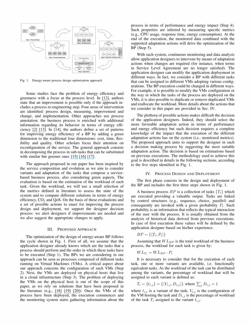
Fig. 1. Energy-aware process design optimization approach

Some studies face the problem of energy efficiency andgreenness with a focus at the process level. In [12], authorsstate that an improvement is possible only if the approach in-cludes a process re-engineering step. Four areas of interventionare identified: process design, measuring, improvement andchange, and implementation. Other approaches use processannotation: the business process is enriched with additionalinformation regarding its behavior in terms of energy effi-ciency [2] [13]. In [14], the authors define a set of patternsfor improving energy efficiency of a BP by adding a greendimension to the traditional four dimensions: cost, time, flex-ibility and quality. Other scholars focus their attention onreconfiguration of the service. The general approach consistsin decomposing the process in sub-tasks that can be substitutedwith similar but greener ones [15] [16] [17].

The approach proposed in our paper has been inspired bythe service composition and evolution as we aim to considervariants and adaptation of the tasks that compose a service-based business process, also considering green aspects. Theevaluation is based on the estimation of the workload of eachtask. Given the workload, we will use a small selection ofthe metrics defined in literature to assess the state of thesystem and to compare different solutions in terms of energyefficiency, CO2 and QoS. On the basis of these evaluations anda set of possible actions to enact for improving the processdesign and deployment, we support the designer decisionprocess: we alert designers if improvements are needed andwe also suggest the appropriate changes to apply.

III. PROPOSED APPROACH

The optimization of the design of energy-aware BP followsthe cycle shown in Fig. 1. First of all, we assume that theapplication designer already knows which are the tasks that aprocess should perform and the order in which these tasks haveto be executed (Step 1). The BPs we are considering in ourapproach can be seen as processes composed of different tasksrunning on Virtual Machines (VMs). A critical aspect aboutour approach concerns the configuration of such VMs (Step2). Next, the VMs are deployed on physical hosts that livein a cloud infrastructure (Step 3). The problem of deployingthe VMs on the physical host is out of the scope of thispaper, as we rely on solutions that have been proposed inthe literature (e.g., [18] [19] [20]). Once the VMs of theprocess have been deployed, the execution commences andthe monitoring system starts gathering information about the

process in terms of performance and energy impact (Step 4).Such properties are inferred by measuring specific metrics(e.g., CPU usage, response time, energy consumption). At theend of the execution, the monitored data combined with thesupported adaptation actions will drive the optimization of theBP (Step 5).

With such system, continuous monitoring and data analysisallow application designers to intervene by means of adaptationactions when changes are required (for instance, when termsin Service Level Agreement are no longer satisfied). Theapplication designer can modify the application deployment indifferent ways. In fact, we consider a BP with different tasksthat can be assigned to different VMs adopting various config-urations. The BP execution could be changed in different ways.For example, it is possible to modify the VMs configuration orthe way in which the tasks of the process are deployed on theVMs, it is also possible to duplicate or remove duplicated VMsand reallocate the workload. More details about the actions thatwe consider in this paper are provided in Sec. IV.

The plethora of possible actions makes difficult the decisionof the application designers. Indeed, they should select themore favorable adaptation action in terms of performanceand energy efficiency but such decision requires a completeknowledge of the impact that the execution of the differentadaptation actions has on the system (i.e., monitored metrics).The proposed approach aims to support the designer in sucha decision making process by suggesting the most suitableadaptation action. The decision is based on estimations basedon previous executions. The methodology used to achieve thisgoal is described in details in the following sections, accordingto the five steps identified in Fig. 1.

IV. PROCESS DESIGN AND DEPLOYMENT

The first phase consists in the design and deployment ofthe BP and includes the first three steps shown in Fig. 1.

A business process BP is a collection of tasks {Ti} whichare executed providing a valuable output. Tasks are linkedby control structures (e.g., sequence, choice, parallel) andconsequently are invoked with a given probability Pi. Suchprobability is an information that reflects the typical interactionof the user with the process. It is usually obtained from theanalysis of historical data derived from previous executions.In case of first execution these values will be defined by theapplication designer based on his/her experience.

BP = {hTi, Pii}Assuming that WLBP is the total workload of the business

process, the workload for each task is given by:

WLTi = WLBP · Pi

It is necessary to consider that for the execution of eachtask, one or more variants are available, i.e. functionallyequivalent tasks. As the workload of the task can be distributedamong the variants, the percentage of workload that will beassigned to each variant is defined as:

Ti = {ti,j} = {hVi,j , Di,ji} whereP

j Di,j = 1

where ti,j is a variant of the task, Vi,j is the configuration ofthe VM hosting the task and Di,j is the percentage of workloadof the task Ti assigned to the variant ti,j .

A configuration of a task variant consists of a specificconfiguration of the VM on which the task runs. This meansthat the same task can run on different VMs:

Vi,j = hqCPU, qRAM, qStorageiwhere qCPU , qRAM , and qStorage indicates the number

of CPUs, the amount of memory, and the amount of storageavailable for the VM on which the task runs.

In our approach, the distribution among the variants of thesame task, is supported by the optimization algorithm proposedSec. VI. This distribution will affect the workload submittedto each variant for a given task as:

WLti,j = WLTi ·Di,j

In the process deployment phase, each variant ti,j isassigned to a dedicated VMi,j , taking into account its con-figuration Vi,j :

ti,jassigned to�������! VMi,j

and each VM is than deployed on a physical server PHl:

VMi,jdeployed on��������! PHl

As a consequence of the adoption of variants at task level,also variants at business process level can be defined as theapplication of one or more adaptation actions Az . An action Az

is a complex action originated from the composition of one ormore atomic actions over the BP. An action can be expressedas Az = {az,v}, where az,v has an impact on a singletask belonging to the business process. We can define atomicactions as az,v 2 {Add(ti,x), Del(ti,x),Mod(ti,y, ti,x)} ,where:

Add(ti,x) : Ti ! T 0i where T 0

i = Ti [ ti,x ^P

j D0i,j = 1

Del(ti,x) : Ti ! T 0i where T 0

i = Ti � ti,x ^P

j D0i,j = 1

Mod(ti,y, ti,x) : Del(ti,y) +Add(ti,x)

In addition to these actions, also the Nop action has to beconsidered as the application designer can decide to avoid anymodifications.

Thus, applying a composite action Az to a business processBP we obtain a variant BP 0 consisting in a different set oftask variants and in a different workload distribution amongthem: i.e., BP

Az��! BP 0z . Thus, the goal of the optimization

described in Sec. VI is to identify the variant that betterimproves both the performances of the process and the en-ergy efficiency assessed by using the metrics introduced inSection V.

V. PROCESS EXECUTION AND MONITORING

Monitoring is fundamental to gather data about perfor-mance and energy efficiency of an application. Such propertiesare inferred by measuring specific metrics. In details, the setof metrics considered in this work includes:

• VM resource usage parameters: CPU and memoryutilization percentages for a running application overa run time interval are calculated by using the ratio be-tween the amount of used and allocated CPU/memory.The resource usage parameters also include IOPS that

is defined as the total number of I/O operations persecond.

• Throughput: number of performed transactions over aperiod of time.

• Energy consumption: refers to the energy consumedby the application in a specific period of time.

• CO2 emissions: quantity of CO2 emitted by executingthe specific application.

• Application performance: is the ratio between thethroughput of the VM in a certain time interval andthe energy consumed.

• Response time: refers to the time spent to serve asingle request.

More formally, each metric can be modeled as:

mh =< name, V > (1)

where the name identifies the metric and V corresponds to theset of admissible values. It is represented by its extremes, i.e.,V = [vmin, vmax].

Metrics can be collected at the BP level or at the VM/taskvariant level. For each of these levels, users can operate arestriction on the admissible range of values for each mh, in or-der to require a specific energy consumption, or performance.This restriction can be formalized as:

rh(c) =< mh, req, w > (2)

where c 2 {BP, {VMi,j}}, and req 2 mh.V . More precisely,req represents the restriction on the range of admissiblevalues for metric mh computed over the component c. Thisrestriction corresponds to the values required by the userfor the given metric. Finally w 2 [0, 1] is the weight thatdefines the relevance of the metric for the specific user (orapplication) and provides a prioritization of the requirements.Such requirements and constraints can be used to derive theinitial deployment of applications as well as provide impetusfor run-time adaptation of application deployment. Note thatthe constraints can be hard constraints if the user considersthat they must be satisfied or soft constraints if the user alsoaccepts a constraint violation. Note that for the hard constraintthe relevance weight will be rh(c).w = 1 while for the softconstraints rh(c).w 1.

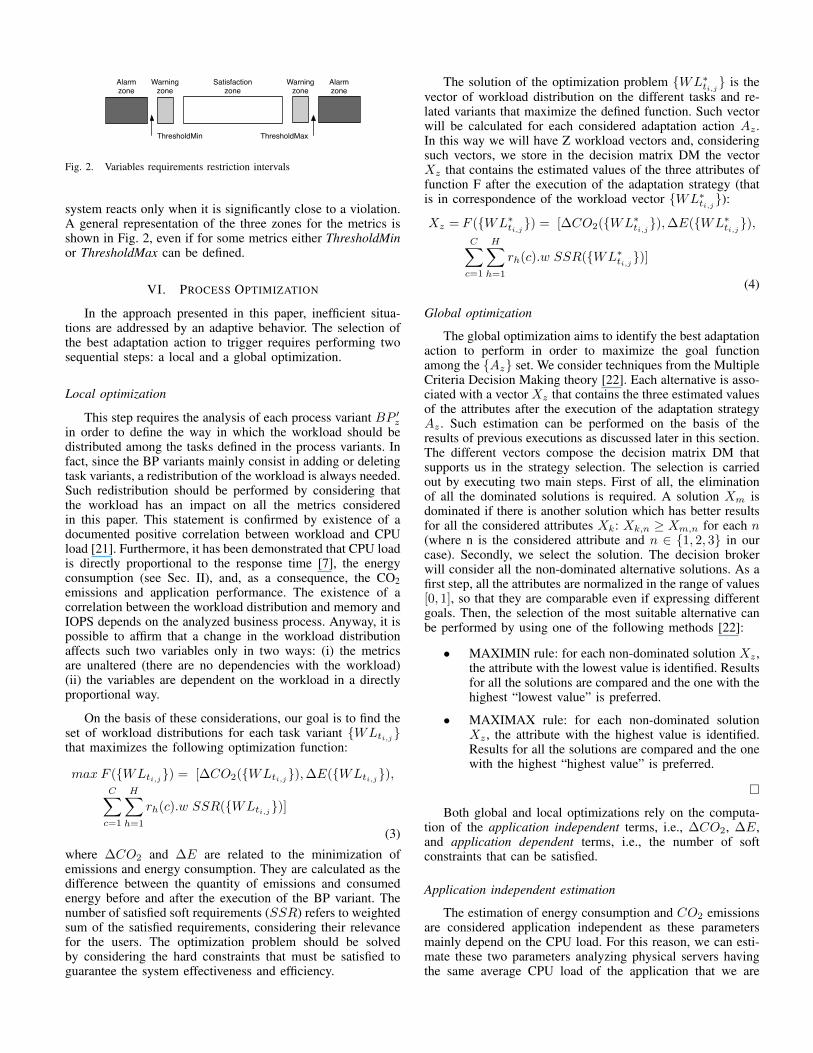
Setting the set of values mh(c).req, the users identifiesthe values related to desired (satisfaction zone) and undesired(alarm zone) behavior for each metric. Also a warning zoneis defined slightly before the alarm zone, and its range ofvalues is identified automatically on the basis of the designerrequirements. In fact, such a range of values depends onthe strategy that the designer wants to adopt for the systemimprovement. Two possible approaches are possible: proactiveand reactive. Adopting a proactive approach implies that awarning is triggered before reaching a real violation, so thatthe system can react in advance. It requires the usage of anextended warning zone between the satisfaction and the alarmzone. On the contrary, using a reactive approach implies awarning zone very close to the alarm threshold. In this case the

Alarmzone

Warningzone

Satisfactionzone

Alarmzone

Warningzone

ThresholdMin ThresholdMax

Fig. 2. Variables requirements restriction intervals

system reacts only when it is significantly close to a violation.A general representation of the three zones for the metrics isshown in Fig. 2, even if for some metrics either ThresholdMinor ThresholdMax can be defined.

VI. PROCESS OPTIMIZATION

In the approach presented in this paper, inefficient situa-tions are addressed by an adaptive behavior. The selection ofthe best adaptation action to trigger requires performing twosequential steps: a local and a global optimization.

Local optimization

This step requires the analysis of each process variant BP 0z

in order to define the way in which the workload should bedistributed among the tasks defined in the process variants. Infact, since the BP variants mainly consist in adding or deletingtask variants, a redistribution of the workload is always needed.Such redistribution should be performed by considering thatthe workload has an impact on all the metrics consideredin this paper. This statement is confirmed by existence of adocumented positive correlation between workload and CPUload [21]. Furthermore, it has been demonstrated that CPU loadis directly proportional to the response time [7], the energyconsumption (see Sec. II), and, as a consequence, the CO2emissions and application performance. The existence of acorrelation between the workload distribution and memory andIOPS depends on the analyzed business process. Anyway, it ispossible to affirm that a change in the workload distributionaffects such two variables only in two ways: (i) the metricsare unaltered (there are no dependencies with the workload)(ii) the variables are dependent on the workload in a directlyproportional way.

On the basis of these considerations, our goal is to find theset of workload distributions for each task variant {WLti,j}that maximizes the following optimization function:

max F ({WLti,j}) = [�CO2({WLti,j}),�E({WLti,j}),CX

c=1

HX

h=1

rh(c).w SSR({WLti,j})]

(3)where �CO2 and �E are related to the minimization ofemissions and energy consumption. They are calculated as thedifference between the quantity of emissions and consumedenergy before and after the execution of the BP variant. Thenumber of satisfied soft requirements (SSR) refers to weightedsum of the satisfied requirements, considering their relevancefor the users. The optimization problem should be solvedby considering the hard constraints that must be satisfied toguarantee the system effectiveness and efficiency.

The solution of the optimization problem {WL⇤ti,j} is the

vector of workload distribution on the different tasks and re-lated variants that maximize the defined function. Such vectorwill be calculated for each considered adaptation action Az .In this way we will have Z workload vectors and, consideringsuch vectors, we store in the decision matrix DM the vectorXz that contains the estimated values of the three attributes offunction F after the execution of the adaptation strategy (thatis in correspondence of the workload vector {WL⇤

ti,j}):

Xz = F ({WL⇤ti,j}) = [�CO2({WL⇤

ti,j}),�E({WL⇤ti,j}),

CX

c=1

HX

h=1

rh(c).w SSR({WL⇤ti,j})]

(4)

Global optimization

The global optimization aims to identify the best adaptationaction to perform in order to maximize the goal functionamong the {Az} set. We consider techniques from the MultipleCriteria Decision Making theory [22]. Each alternative is asso-ciated with a vector Xz that contains the three estimated valuesof the attributes after the execution of the adaptation strategyAz . Such estimation can be performed on the basis of theresults of previous executions as discussed later in this section.The different vectors compose the decision matrix DM thatsupports us in the strategy selection. The selection is carriedout by executing two main steps. First of all, the eliminationof all the dominated solutions is required. A solution Xm isdominated if there is another solution which has better resultsfor all the considered attributes Xk: Xk,n � Xm,n for each n(where n is the considered attribute and n 2 {1, 2, 3} in ourcase). Secondly, we select the solution. The decision brokerwill consider all the non-dominated alternative solutions. As afirst step, all the attributes are normalized in the range of values[0, 1], so that they are comparable even if expressing differentgoals. Then, the selection of the most suitable alternative canbe performed by using one of the following methods [22]:

• MAXIMIN rule: for each non-dominated solution Xz ,the attribute with the lowest value is identified. Resultsfor all the solutions are compared and the one with thehighest “lowest value” is preferred.

• MAXIMAX rule: for each non-dominated solutionXz , the attribute with the highest value is identified.Results for all the solutions are compared and the onewith the highest “highest value” is preferred.

⇤Both global and local optimizations rely on the computa-

tion of the application independent terms, i.e., �CO2, �E,and application dependent terms, i.e., the number of softconstraints that can be satisfied.

Application independent estimation

The estimation of energy consumption and CO2 emissionsare considered application independent as these parametersmainly depend on the CPU load. For this reason, we can esti-mate these two parameters analyzing physical servers havingthe same average CPU load of the application that we are

going to deploy, regardless of the applications that are actuallyrunning.

In order to evaluate the factor �E({WLti,j}), for eachWLti,j , first we consider logs of previous executions of thetask variant ti,j in order to find the relationships betweenworkload and CPU load. Thus, given a WLti,j we retrievethe correspondent CPULoad(ti,j). Once we have this valueand we know the characteristics of the physical host PHl (i.e.,peak power) on which the VMi,j is deployed, we estimate theenergy by gathering the power consumed by a similar taskdeployed on a similar host. Such a similarity is computedby comparing the CPU load of the analyzed task and thecharacteristics of the host where it runs, to the hystorical dataof the hosts usage, looking for hosts with similar characteristicsthat run applications with a similar CPU load.

The evaluation of the CO2 emissions is based on theemission factors (gCO2e/kWh) provided by the national grids.Considering the consumed energy E(ti,j) CO2 emissions iscomputed multiplying the energy consumed by the emissionfactor.

Application dependent estimation

In this section we estimate the last part of the objectivefunction described in Eq. 3, i.e., the number of metrics thatwill be satisfied SSR.

As before, we try to predict the trends of the state ofthe variables for a given distribution of the load between theavailable variants of each task. In this case we can not usethe similarity criteria introduced in the previous paragraph.In fact, the value of the variables is strictly dependent onthe application and it is very unlikely to find examples ofthe variables behaviors in historical data for all the possibleconfigurations of the process.

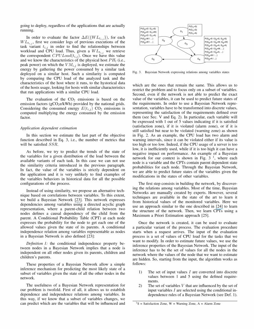
Instead of using similarity, we propose an alternative tech-nique based on correlations between variables. To this extent,we build a Bayesian Network [23]. This network expressesdependencies among variables using a directed acyclic graphrepresentation, where a parent-child relation between twonodes defines a causal dependency of the child from theparent. A Conditional Probability Table (CPT) at each nodeexpresses the probability for the node to get each one of theallowed values given the state of its parents. A conditionalindependence relation among variables representable as nodesin a Bayesian Network is also defined [23]:

Definition 1: the conditional independence property be-tween nodes in a Bayesian Network implies that a node isindependent on all other nodes given its parents, children andchildren’s parents.

These properties of a Bayesian Network allow a simpleinference mechanism for predicting the most likely state of asubset of variables given the state of all the other nodes in thenetwork.

The usefulness of a Bayesian Network representation forour problem is twofold. First of all, it allows us to establishdependence and independence relations among variables. Inthis way, if we know that a subset of variables changes, wecan predict which are the variables that will be influenced and

G1

G2G3

G5 G4

P(G4=S | G2=S, G3=S)P(G4=S | G2=W, G3=W)P(G4=S | G2=A, G3=A)P(G4=S | G2=W, …)P(G2=S | G2=A, ...)P(G4=W | …)P(G2=A | ...)

P(G1=S)P(G1=S)P(G1=A)

P(G2=S | G1=S)P(G2=S | G1=W)P(G2=S | G1=A)P(G2=W | …)P(G2=W | …)

Fig. 3. Bayesian Network expressing relations among variables states

which are the ones that remain the same. This allows us torestrict the problem and to focus only on a subset of variables.Second, even if the network is not able to predict the exactvalue of the variables, it can be used to predict future states ofthe requirements. In order to use a Bayesian Network repre-sentation, variables have to be transformed into discrete values,representing the satisfaction of the requirements defined overthem (see Sec. V and Eq. 2). In particular, each variable willbe expressed with 1 out of 5 values indicating if it is satisfied(satisfaction zone), if it is violated (alarm zone), or if it isstill satisfied but near to be violated (warning zone) as shownin Fig. 2. As an example, the CPU load has two alarm andwarning intervals, since it can be violated either if its value istoo high or too low. Indeed, if the CPU usage of a server is toolow, it is inefficiently used, while if it is too high it can have anegative impact on performance. An example of a Bayesiannetwork for our context is shown in Fig. 3 1, where eachnode is a variable and the CPTs contain parent dependent stateprobabilities for each node. Through the Bayesian Network,we are able to predict future states of the variables given themodifications in the states of other variables.

The first step consists in building the network, by discover-ing the relations among variables. Most of the time, BayesianNetworks are manually created by experts. However, severaltechniques are available in the state of the art to learn itfrom historical values of the monitored variables. Here weuse an approach similar to the one described in [24] to learnthe structure of the network. Then, we learn CPTs using aMaximum a Priori Estimation approach [25].

Once the network is created, it can be used to evaluatea particular variant of the process. The evaluation procedurestarts when a request arrives. The input of the evaluationprocess is a set of values of CPU load for the tasks that wewant to modify. In order to estimate future values, we use theinference properties of the Bayesian Network. The input of theinference has to be the set of values for all the nodes in thenetwork where the values of the node that we want to estimateare hidden. So, starting from the input, the algorithm works asfollows:

1) The set of input values I are converted into discretevalues between 1 and 5 using the defined require-ments.

2) The set of variables V that are influenced by the set ofinput variables I are selected using the conditional in-dependence rules of a Bayesian Network (see Def. 1).

1S = Satisfaction Zone, W = Warning Zone, A = Alarm Zone

3) An input vector InfInput for the inference proce-dure is defined as follows:

• take the vector with the state of the variablesobtained by the monitoring system.

• modify the values of the variables in I withthe values computed at step 1.

• hide the variables in V from the vector.4) Run inference with input vector InfInput obtaining

the most likely states for each variable in V associ-ated with a probability PV for the variable to get thatstate.

5) Return as output a binary vector InfInput0 obtainedfrom InfInput. A value equals to 1 means that therequirements upon the variable are satisfied, while avalue equals to 0 means that they are violated. Anadditional vector Conf of the same dimension isalso created with the values PV for each predictedvariable. The probability value for all the variablesthat do not belong to V will be 1, because they areconsidered as constant.

The probability value returned by the inference procedureis used as a confidence parameter in the estimation of the valuefor the third attribute of the optimization function.

VII. VALIDATION

To provide a validation of our approach, we consider asample BP (see Fig. 4), where a set of tasks are performed tobuy goods using an e-commerce Web site. This BP involvesseveral VMs where the tasks are installed and executed. Usingthe notation introduced in Sec. IV, our BP is defined as:

BP = {hBS, 1.0i, hRO, 0.90i, hV O, 0.95i, (5)hRP, 0.855i, hIP, 0.855i hCA, 0.045i}

To execute the business process and monitor the metrics intro-duced in Section III, we relied on the BonFIRE infrastructure2.For the sake of simplicity, and considering that the BonFIREplatform is not now able to monitor the energy related metricsand the I/O usage:

• As the memory usage does not change significantlyduring the experiment, in this validation we focus onthe CPU Usage.

• For the energy-related metrics, we rely on the resultspublished in [8] to estimate the power of a physicalhost based on the CPU load.

• We assume that each task of the BP lives on adedicated VM and that the resulting VMs are deployedon different physical hosts.

• Although on a physical host, in addition to our VMs,other VMs of other applications are running, weassume that the CPU load of these external VMsremains constant as we are interested in the variationof consumption of our business process.

• The VMs can be hosted on data centers sited in Franceand England where the average CO2 emission fac-

2http://www.bonfire-project.eu/

tors are, respectively, 146 gCO2e/kWh 3 and 567.17gCO2e/kWh 4.

The two possible configurations of the VM used for ourvalidation are:

• VM2,2 = h 2 cores, 2 GBytes, 10Gbytes i.• VM4,4 = h 4 cores, 4 GBytes, 10Gbytes i.

where a Linux Debian Squeeze v.5 distribution is installed,along with Oracle Glassfish v3.1 to run the activities compos-ing our BP.

Creating the Bayesian Network

The creation of the Bayesian Network requires a knowledgeabout previous executions of the BP. At least during the firstdesign of our BP this kind of information is not available.Nevertheless, as common behavior in case of service-basedbusiness processes, we can assume that other instances of thesame tasks composing our BP have been previously used inother processes.

Starting from the historical data collected from the moni-toring system, and using the procedure described in Sec. VI,we obtain a Bayesian Network describing the relations amongvariables in the system. We consider to have metrics at twolevels:

• Task Level: metrics at this level are CPU load (CPU)of the VM, throughput (TH) and response time (RT)of the task variant running on the VM.

• BP level: metrics at this level are response time (RT),throughput (TH), and application performance (AP) ofthe whole process.

The network obtained for the considered example is shownin Fig. 5, representing a simplified version of the real network.In the picture, only a general task is represented, while in thereal network the same structure is replicated for each of thetasks and their variants in the BP. In our example, we havesix tasks. The response time of all the tasks and their variantscontribute to the response time of the whole process, and thesame can be stated for the throughput.

Initial configuration

The application designer decides to initially run the sixtasks on six VMs having the same configuration (i.e., theVM2,2). For these VMs, the designer initially does not addany variant, so the workload of a given task is entirely sent tothe unique available VMs, thus:

BS = RO = V O = RP = IP = CA = hVM2,2, 1.0iAs hard constraint, we have RT (BP ) 25min. As soft

constraints, we have:• 8 Ti [70% CPU(Ti) 90% ; RT (Ti)]

• TH(BP ) � 5tpm

• AP (BP ) � 8.5tpKWh.

3http://www.eumayors.eu/IMG/pdf/seap guidelines en.pdf4http://www.defra.gov.uk/publications/

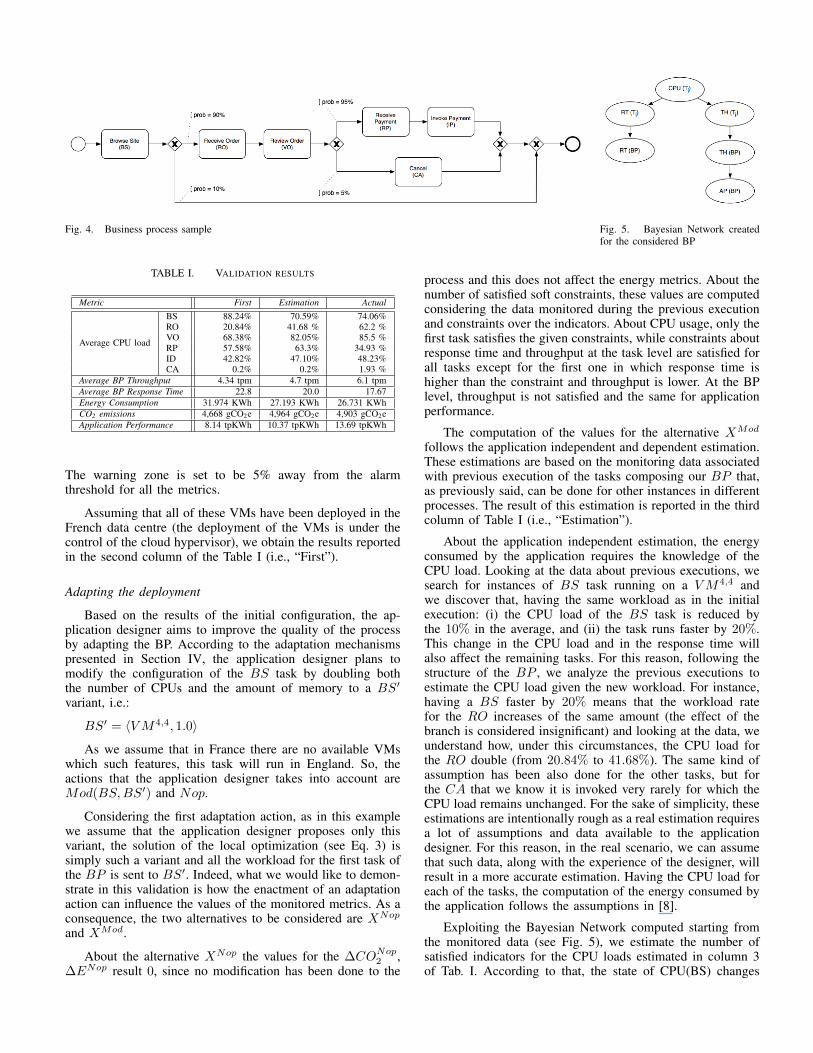
Fig. 4. Business process sample Fig. 5. Bayesian Network createdfor the considered BP

TABLE I. VALIDATION RESULTS

Metric First Estimation Actual

Average CPU load

BS 88.24% 70.59% 74.06%RO 20.84% 41.68 % 62.2 %VO 68.38% 82.05% 85.5 %RP 57.58% 63.3% 34.93 %ID 42.82% 47.10% 48.23%CA 0.2% 0.2% 1.93 %

Average BP Throughput 4.34 tpm 4.7 tpm 6.1 tpmAverage BP Response Time 22.8 20.0 17.67Energy Consumption 31.974 KWh 27.193 KWh 26.731 KWhCO2 emissions 4,668 gCO2e 4,964 gCO2e 4,903 gCO2eApplication Performance 8.14 tpKWh 10.37 tpKWh 13.69 tpKWh

The warning zone is set to be 5% away from the alarmthreshold for all the metrics.

Assuming that all of these VMs have been deployed in theFrench data centre (the deployment of the VMs is under thecontrol of the cloud hypervisor), we obtain the results reportedin the second column of the Table I (i.e., “First”).

Adapting the deployment

Based on the results of the initial configuration, the ap-plication designer aims to improve the quality of the processby adapting the BP. According to the adaptation mechanismspresented in Section IV, the application designer plans tomodify the configuration of the BS task by doubling boththe number of CPUs and the amount of memory to a BS0

variant, i.e.:

BS0 = hVM4,4, 1.0i

As we assume that in France there are no available VMswhich such features, this task will run in England. So, theactions that the application designer takes into account areMod(BS,BS0) and Nop.

Considering the first adaptation action, as in this examplewe assume that the application designer proposes only thisvariant, the solution of the local optimization (see Eq. 3) issimply such a variant and all the workload for the first task ofthe BP is sent to BS0. Indeed, what we would like to demon-strate in this validation is how the enactment of an adaptationaction can influence the values of the monitored metrics. As aconsequence, the two alternatives to be considered are XNop

and XMod.

About the alternative XNop the values for the �CONop2 ,

�ENop result 0, since no modification has been done to the

process and this does not affect the energy metrics. About thenumber of satisfied soft constraints, these values are computedconsidering the data monitored during the previous executionand constraints over the indicators. About CPU usage, only thefirst task satisfies the given constraints, while constraints aboutresponse time and throughput at the task level are satisfied forall tasks except for the first one in which response time ishigher than the constraint and throughput is lower. At the BPlevel, throughput is not satisfied and the same for applicationperformance.

The computation of the values for the alternative XMod

follows the application independent and dependent estimation.These estimations are based on the monitoring data associatedwith previous execution of the tasks composing our BP that,as previously said, can be done for other instances in differentprocesses. The result of this estimation is reported in the thirdcolumn of Table I (i.e., “Estimation”).

About the application independent estimation, the energyconsumed by the application requires the knowledge of theCPU load. Looking at the data about previous executions, wesearch for instances of BS task running on a VM4,4 andwe discover that, having the same workload as in the initialexecution: (i) the CPU load of the BS task is reduced bythe 10% in the average, and (ii) the task runs faster by 20%.This change in the CPU load and in the response time willalso affect the remaining tasks. For this reason, following thestructure of the BP , we analyze the previous executions toestimate the CPU load given the new workload. For instance,having a BS faster by 20% means that the workload ratefor the RO increases of the same amount (the effect of thebranch is considered insignificant) and looking at the data, weunderstand how, under this circumstances, the CPU load forthe RO double (from 20.84% to 41.68%). The same kind ofassumption has been also done for the other tasks, but forthe CA that we know it is invoked very rarely for which theCPU load remains unchanged. For the sake of simplicity, theseestimations are intentionally rough as a real estimation requiresa lot of assumptions and data available to the applicationdesigner. For this reason, in the real scenario, we can assumethat such data, along with the experience of the designer, willresult in a more accurate estimation. Having the CPU load foreach of the tasks, the computation of the energy consumed bythe application follows the assumptions in [8].

Exploiting the Bayesian Network computed starting fromthe monitored data (see Fig. 5), we estimate the number ofsatisfied indicators for the CPU loads estimated in column 3of Tab. I. According to that, the state of CPU(BS) changes

from warning to satisfied and CPU(VO) changes from alarmto warning. All other values for CPU(Ti) are not affected. Thisimpact RT(BS) and TH(BS), now having a high probabilityof being satisfied, while RT(VO) and TH(VO) were alreadysatisfied and the improvement of CPU(VO) does not changethis state. The modification of RT(BS) and TH(BS) affects pos-itively TH(BP) with a consequent improvement of AP(BP). Asa consequence, the total count of satisfied indicators increasesof 5, counting indicators in the warning state as satisfied.The hard requirements about RT(BP), already satisfied in theprevious configuration, is still satisfied.

As a consequence, the values of the objective function forthe two alternatives are:

XNop = (�CONop2 ,�ENop,#SSRNop) = (0, 0, 12)

XMod = (�COMod2 ,�EMod,#SSRMod) = (�296, 4.78, 17)

As can be observed, neither of the two solutions is dominant.In order to decide the best of the two, one of the techniquesdescribed in Sec. VI has to be applied. For example, usingthe MAXIMIN approach, firstly, for each alternative the min-imum value among the three attributes is considered, i.e., forXNop action min(0, 0, 12) = 0 while for the XMod actionmin(�296, 4.78, 17) = �296. Secondly, the solution to preferis the one that is associated with the highest number: in ourcase the maximum between 0 and �296 is 0 and then theXNop solution is considered as suitable (i.e., doing nothing).This reflects the higher importance given at the CO2 emissionswith respect to the performance and energy consumption.

VIII. FINAL REMARKS

In this paper we presented an approach for supporting theenergy-aware adaptation of business processes at design timedriven by an optimization problem that takes into account bothinfrastructural, applicative, and environmental standpoints. Inparticular, the adaptation actions available to the applicationdesigner rely on the definition of variants for the tasks com-posing the business process.

This approach is now heavily based on the assumption thatmonitored data about previous executions are available, andinformation able to give the values for the interesting metricsare all included in this knowledge base. For future developmentof our approach, we aim to relax this assumption, trying tounderstand if we can infer the values of the metrics in casethe data needed to compute them analytically are not present.

ACKNOWLEDGMENT

This work has been supported by the ECO2Clouds project(http://eco2clouds.eu/) and has been partly funded by theEuropean Commission’s IST activity of the 7th FrameworkProgramme under contract number 318048.

REFERENCES

[1] Greenpeace, “How Clean Is Your Cloud?,” tech. rep., 04 2012.[2] A. Nowak, F. Leymann, D. Schumm, and B. Wetzstein, “An architecture

and methodology for a four-phased approach to green business processreengineering,” in Proceedings of ICT-GLOW 2011, Toulouse, France,vol. 6868 of LNCS, pp. 150–164, Springer-Verlag, 2011.

[3] A. Kipp, T. Jiang, M. Fugini, and I. Salomie, “Layered green perfor-mance indicators,” Future Generation Computer Systems, vol. 28, no. 2,pp. 478–489, 2012.

[4] R. P. Larrick and K. W. Cameron, “Consumption-Based Metrics: FromAutos to IT,” Computer, pp. 97–99, 2011.

[5] D. Chen, E. Henis, C. Cappiello, et al., “Usage centric green perfor-mance indicators,” in Proceedings of the Green Metrics 2011 Workshop(in conjunction with ACM SIGMETRICS 2011), 2010.

[6] D. Meisner, B. T. Gold, and T. F. Wenisch, “Powernap: eliminatingserver idle power,” in Proc. of the 14th Int’l conference on Architecturalsupport for programming languages and operating systems, ASPLOSXIV, (New York, NY, USA), pp. 205–216, ACM, 2009.

[7] M. Pedram and I. Hwang, “Power and Performance Modeling in aVirtualized Server System,” in Parallel Processing Workshops (ICPPW),2010 39th International Conference on, pp. 520–526, 2010.

[8] D. Kliazovich, P. Bouvry, and S. U. Khan, “Greencloud: a packet-levelsimulator of energy-aware cloud computing data centers,” The Journalof Supercomputing, pp. 1–21, 2010.

[9] D. Borgetto, M. Maurer, G. Da-Costa, J.-M. Pierson, and I. Brandic,“Energy-efficient and sla-aware management of iaas clouds,” in Pro-ceedings of the 3rd International Conference on Future Energy Systems:Where Energy, Computing and Communication Meet, p. 25, 2012.

[10] G. Katsaros, J. Subirats, J. Oriol Fito, J. Guitart, P. Gilet, and D. Espling,“A service framework for energy-aware monitoring and VM manage-ment in Clouds,” Future Generation Computer Systems, 2012.

[11] A. Beloglazov, R. Buyya, Y. C. Lee, and A. Zomaya, “A taxonomy andsurvey of energy-efficient data centers and cloud computing systems,”Advances in Computers, vol. 82, no. 2, pp. 47–111, 2011.

[12] S. Seidel, J. vom Brocke, and J. C. Recker, “Call for Action: Investigat-ing the Role of Business Process Management in Green IS,” Sprouts:Working Papers on Information Systems, vol. 11, no. 4, 2011.

[13] C. Cappiello, M. G. Fugini, A. M. Ferreira, P. Plebani, and M. Vitali,“Business Process Co-Design for Energy-Aware Adaptation,” in Intel-ligent Computer Communication and Processing (ICCP), 2011 IEEEInternational Conference on, pp. 463–470, 2011.

[14] A. Nowak, F. Leymann, D. Schleicher, D. Schumm, and S. Wagner,“Green Business Process Patterns,” in Proceedings of the 18th Confer-ence on Pattern Languages of Programs, ACM, 2011.

[15] K. Hoesch-Klohe and A. Ghose, “Carbon-Aware Business ProcessDesign in Abnoba,” Service-Oriented Computing, pp. 551–556, 2010.

[16] A. Mello Ferreira, K. Kritikos, and B. Pernici, “Energy-Aware Designof Service-Based Applications,” Service-Oriented Computing, pp. 99–114, 2009.

[17] A. De Oliveira, G. Frederico, and T. Ledoux, “Self-optimisation of theenergy footprint in service-oriented architectures,” Proceedings of the1st Workshop on Green Computing (GCM’10), 2010.

[18] A. Beloglazov and R. Buyya, “Energy efficient resource managementin virtualized cloud data centers,” in Proceedings of the 2010 10thIEEE/ACM International Conference on Cluster, Cloud and Grid Com-puting, CCGRID ’10, pp. 826–831, 2010.

[19] G. Dhiman, G. Marchetti, and T. Rosing, “vgreen: a system for energyefficient computing in virtualized environments,” in Proceedings of the14th ACM/IEEE international symposium on Low power electronics anddesign, ISLPED ’09, pp. 243–248, 2009.

[20] A. Younge, G. von Laszewski, L. Wang, S. Lopez-Alarcon, andW. Carithers, “Efficient resource management for cloud computingenvironments,” in Green Computing Conference, 2010 International,pp. 357–364, 2010.

[21] A. Verma, G. Dasgupta, T. K. Nayak, P. De, and R. Kothari, “Serverworkload analysis for power minimization using consolidation,” inProceedings of the 2009 conference on USENIX Annual technicalconference, USENIX’09, (Berkeley, CA, USA), pp. 28–28, USENIXAssociation, 2009.

[22] E. Triantaphyllou, Multi-Criteria Decision Making Methods: A compar-ative Study. Springer, 2004.

[23] S. J. Russell, P. Norvig, and E. Davis, Artificial intelligence: a modernapproach, vol. 2. Prentice hall Englewood Cliffs, 2010.

[24] I. Tsamardinos, L. E. Brown, and C. F. Aliferis, “The max-minhill-climbing bayesian network structure learning algorithm,” Machinelearning, vol. 65, no. 1, pp. 31–78, 2006.

[25] R. E. Neapolitan, Learning bayesian networks. Pearson Prentice HallUpper Saddle River, 2004.