Import demand of bananas in the European Union

Authors

Chacón-Cascante, Adriana Ph.D. Student

Agricultural Economics Department Kansas State University

achacon@agecon.ksu.edu

Marsh, Thomas Lloyd, Ph.D. Associate Professor, School of Economic Sciences

Washington State University tl_marsh@wsu.edu

Crespi, John Associate Professor

Agricultural Economics Department Kansas State University jcrespi@agecon.ksu.edu

Selected Paper presented for presentation at the American Economics Asociation Annual

Meeting, Providence, Rhode Island, July 24-27. 2005

Copyright 2005by Adriana Chacón-Cascante, Thomas Marsh and John Crepi. Readers may make verbatim copies of this document for non-commercial purposes by any means, provided that this copyright notice appears on all such copies.

2

Import demand of bananas in the EU

The EU banana market has been of enormous interest for researchers for a long time. Prior to

the policy unification brought by the Common Market Organization for Bananas (CMOB),

many authors studied the implications of the multi policy scheme prevalent before 1993. This

interest derived from the distorting effects of those import policies not only within the EU but

also in the world banana market. The interest for studying the EU banana situation increased

with the CMOB. Several factors contributed to this but probably the main reason was the

adverse reactions generated by this policy in different sectors.

For example, some argue the EU protected certain low-income countries to the

detriment of other developing nations that were also highly dependent on banana trade.

Additionally, the aid system that accompanied the import regime was highly inefficient. Only a

small proportion of the money intended to compensate preferred suppliers for any loss derived

from the import system actually reached its target. The issue about the EU banana market

became even more complicated when the interests of US multinational fruit companies entered

the scenario. The interest for the European Union banana market resumed with the endorsement

of the banana agreement between the EU and the United States in 2002.

What is interesting about the many analyses of this market is that the conclusions

reached by them vary considerably. Divergences in the results are found not only in the

magnitude of the effects but also in the way the involved parties have been affected by the

alternative import policies. One of the main reasons for those discrepancies is that for each

evaluation, a different set of demand parameters has been used. A common denominator to the

estimations used is that the general demand restrictions necessary to make them consistent with

3

economic theory has not been incorporated. Table 1 summarizes a few of the demand elasticity

set ups and the welfare effects that some authors have estimated for the EU banana market.

It is obvious from those results that demand parameters highly affect the results

obtained from the welfare analysis. Now, that a new banana import agreement has emerged in

the EU, an adequate estimation of its import demand becomes relevant from a policy analysis

perspective. The objective of this project is to estimate a well-defined demand system to

generate reliable elasticities to facilitate future welfare analysis of the EU banana market.

Simulations to calculate preliminary welfare effects of the new import regime on Latin

American producers and on EU consumers of bananas from this region are also performed.

The paper is organized in two main sections. Section one presents the methodology

used to estimate the import demand elasticities for bananas in the EU. The results obtained are

summarized and discussed. Section two deals with the welfare estimations for the new import

regime that the EU intends to bring in January 2006. The welfare analysis centers on the Latin

American region, therefore, just changes in the wellbeing of producers from that region and in

EU consumers of Latin American bananas are estimated.

4

Table 1. Summary of some demand elasticities and welfare analysis of previous evaluations of the EU banana market.

Source Method for calculating elasticities Comparison period Welfare cost for EU consumers(a)

Borell and Yang (1990) Elasticities assumed Before 1993 693

Matthews (1992) Elasticities assumed based on prior

studies

Before 1993 579

Borell and Cuthbertson quoted

in Matthews 1992

Elasticities assumed Before 1993 1438

Borell and Yang (1992) Elasticities assumed Before 1993 1610

McInerney and Person (1992) Before 1993 1600

Read (1994) Unpublished Before 1993 642

Borell (1994) Elasticities assumed After 19993 2300

Euro PA (1995) Same as Borell (1994) After 19993 800-1000

Source: H. Kox,

(a) Million US$

5

Banana import demand elasticities in the European Union

Initially, two different models were estimated for determining whether a regular o an inverse

demand system better fitted the way the EU banana market behaves. The first corresponded to

the almost ideal demand system (AIDS), under the usual assumption that quantities imported

are determined by the import price. This is the demand definition used by most researchers.

The second model corresponded to the inverse almost ideal demand system (IAIDS) which

assumes that prices adjust to quantities. This assumption was reasonable under the current

import scheme, when imports are limited by quotas. However, with the forthcoming

elimination of all quotas in January 2006, that will not longer be the case.

Total supply of bananas en the EU is decomposed into four components, each

representing a different supplier region. The first corresponds to Latin America, the main

supplier of the EU. The second is composed of the countries from Africa, the Caribbean and

Pacific that has traditionally enjoyed preference access to the EU market. The third region

comprises the communitarian countries, which are mainly overseas territories of Greece, Spain,

France and Portugal. Finally, the last exporting region comprises all other countries (rest of the

world).

The almost ideal demand system can be obtained from an indirect utility function,

V(p,m), of the form shown in (1):

)(ln)(ln)ln(),(

pbpaIIpV −

= (1)

Where

∑ ∑∑= = =

++=n

i

n

i

n

jjiiji ppppa

1 1 1

*0 lnln5.0)ln()(ln γαα (2)

6

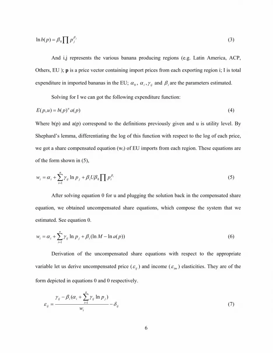
∏= jjppb ββ0)(ln (3)

And i,j represents the various banana producing regions (e.g. Latin America, ACP,

Others, EU ); p is a price vector containing import prices from each exporting region i; I is total

expenditure in imported bananas in the EU; 0α , iα , ijγ and iβ are the parameters estimated.

Solving for I we can got the following expenditure function:

)()(),( papbupE u= (4)

Where b(p) and a(p) correspond to the definitions previously given and u is utility level. By

Shephard’s lemma, differentiating the log of this function with respect to the log of each price,

we got a share compensated equation (wi) of EU imports from each region. These equations are

of the form shown in (5),

∑ ∏=

++=n

iiijijii

ipUpw1

0ln βββγα (5)

After solving equation 0 for u and plugging the solution back in the compensated share

equation, we obtained uncompensated share equations, which compose the system that we

estimated. See equation 0.

))(ln(lnln1∑=

−++=n

iijijii paMpw βγα (6)

Derivation of the uncompensated share equations with respect to the appropriate

variable let us derive uncompensated price ( ijε ) and income ( imε ) elasticities. They are of the

form depicted in equations 0 and 0 respectively.

iji

n

ijijiiij

ij w

pδ

γαβγε −

+−=

∑=1

)ln( (7)

7

1−=i

iim w

βε (8)

Where ijδ is the Kronecker delta, which takes a value of 1 when i=j and zero otherwise.

Compensated elasticities are derived from the above elasticities from the following

relationship:

iMjijcij w εεε −= (9)

These elasticities are meaningful since they are a pure representation of the substitution

relationships between exporting regions. They allows us to exactly determine whether imports

from the different regions are either complementary or substitutes. Finally, to be consistent

with the general demand restrictions, adding up, homogeneity and symmetry were imposed to

the system1.

Data

The data comprise annual observations for the period 1964 to 1999. Trade flows (value and

quantity) are decomposed by exporter country. These data were obtained from the World Trade

Annual of the United Nations. Due to the way the data are reported, it is not possible to

1 0,0,111

=== ∑∑∑==

n

iij

n

ii

n

ii γβα (adding up)

0=∑n

jijγ (homogeneity)

jiij γγ = (symmetry)

8

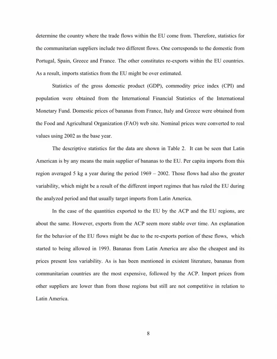
determine the country where the trade flows within the EU come from. Therefore, statistics for

the communitarian suppliers include two different flows. One corresponds to the domestic from

Portugal, Spain, Greece and France. The other constitutes re-exports within the EU countries.

As a result, imports statistics from the EU might be over estimated.

Statistics of the gross domestic product (GDP), commodity price index (CPI) and

population were obtained from the International Financial Statistics of the International

Monetary Fund. Domestic prices of bananas from France, Italy and Greece were obtained from

the Food and Agricultural Organization (FAO) web site. Nominal prices were converted to real

values using 2002 as the base year.

The descriptive statistics for the data are shown in Table 2. It can be seen that Latin

American is by any means the main supplier of bananas to the EU. Per capita imports from this

region averaged 5 kg a year during the period 1969 – 2002. Those flows had also the greater

variability, which might be a result of the different import regimes that has ruled the EU during

the analyzed period and that usually target imports from Latin America.

In the case of the quantities exported to the EU by the ACP and the EU regions, are

about the same. However, exports from the ACP seem more stable over time. An explanation

for the behavior of the EU flows might be due to the re-exports portion of these flows, which

started to being allowed in 1993. Bananas from Latin America are also the cheapest and its

prices present less variability. As is has been mentioned in existent literature, bananas from

communitarian countries are the most expensive, followed by the ACP. Import prices from

other suppliers are lower than from those regions but still are not competitive in relation to

Latin America.

9

Table 2. Data’s descriptive statistics

Variable Mean St. Deviation Variance Minimum MaximumPrices

Latin America 0.292 0.227 0.052 0.000 0.706ACP 0.321 0.269 0.072 0.000 0.725EU 0.356 0.289 0.084 0.026 0.884Others 0.299 0.280 0.078 0.006 0.912

Quantities Latin America 5.077 2.005 4.020 0.000 8.491ACP 1.429 0.456 0.208 0.000 2.348EU 1.352 0.647 0.418 0.048 2.864Others 0.206 0.228 0.052 0.009 0.702

Expenditure 3.038 3.057 9.342 0.007 8.601(1) Prices are US$/kg. (2) Quantities are expressed in per-capita kg

Results

Table 3 presents the parameters obtained from the estimation of the AIDS model. All the

parameters directly obtained from the model were significant at a 5% confidence level, which

makes the elasticity estimated highly reliable. Based on the demand restrictions previously

imposed to the system, values for the eliminated parameters were recovered. These are the

values for which the standard error and the T-ratios are not reported.

10

Table 3. Parameter estimated from the AIDS model for the EU import demand of

bananas

Parameter Coef. St. Error T-Ratio Parameter Coef. St.

Error

T-Ratio

α0 -4502.50 46.68 -96.45 γ23 0.81 0.17 4.80

α1 43.02 10.64 4.04 γ24 -0.52 0.07 -7.16

α2 24.79 1.73 14.33 γ34 2.89 0.61 4.75

α3 -151.30 19.03 -7.95 α4 84.49

β1 -0.01 0.00 -3.90 β4 -0.02

β2 -0.01 0.00 -13.52 γ11 -0.31

β3 0.03 0.00 7.65 γ22 -0.01

γ12 -0.28 0.08 -3.66 γ33 -5.06

γ13 1.37 0.56 2.46 γ 44 -1.59

γ14 -0.78 0.27 -2.86

Uncompensated and income elasticities are shown in Table 4. Income elasticities

indicate that bananas from the Latin America and the ACP regions can be considered normal

goods. However, demand for bananas from these regions increases less than proportionally than

the income of the EU population. Communitarian bananas on the other hand are luxury goods

since their consumption increases more than proportionally than increases in income. Finally,

the income elasticity for the demand from other sources is the close to zero, which makes

bananas from the rest of the world an inferior good for the EU consumers.

The four own price elasticities have the expected negative sign. An important

conclusion that can be drawn from them is that the EU demand for bananas from all regions is

relative inelastic. Import demand from ACP is the least elastic (-0.224), followed by the EU

11

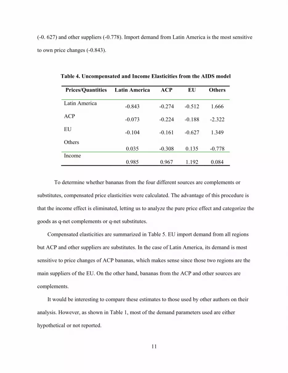
(-0. 627) and other suppliers (-0.778). Import demand from Latin America is the most sensitive

to own price changes (-0.843).

Table 4. Uncompensated and Income Elasticities from the AIDS model

Prices/Quantities Latin America ACP EU Others

Latin America -0.843 -0.274 -0.512 1.666

ACP -0.073 -0.224 -0.188 -2.322

EU -0.104 -0.161 -0.627 1.349

Others 0.035 -0.308 0.135 -0.778

Income 0.985 0.967 1.192 0.084

To determine whether bananas from the four different sources are complements or

substitutes, compensated price elasticities were calculated. The advantage of this procedure is

that the income effect is eliminated, letting us to analyze the pure price effect and categorize the

goods as q-net complements or q-net substitutes.

Compensated elasticities are summarized in Table 5. EU import demand from all regions

but ACP and other suppliers are substitutes. In the case of Latin America, its demand is most

sensitive to price changes of ACP bananas, which makes sense since those two regions are the

main suppliers of the EU. On the other hand, bananas from the ACP and other sources are

complements.

It would be interesting to compare these estimates to those used by other authors on their

analysis. However, as shown in Table 1, most of the demand parameters used are either

hypothetical or not reported.

12

Table 5. Compensated Elasticities from the AIDS model

Latin America ACP EU Others

Latin America -0.2261 0.3515 0.3212 1.5020

ACP 0.0898 -0.0077 -0.0331 -2.4184

EU 0.0874 -0.0352 -0.4653 1.4781

Others 0.0489 -0.3086 0.1771 -0.5617

II. Welfare Analysis

The new import policy proposed by the EU for the import of bananas corresponds to the second

stage of the signed agreement between the EU and the United States. In this stage, which will

come into effect in 2006, exporters will compete on the basis of differentiated tariffs and all

regional or country-specific quotas will be eliminated. The EU has proposed a new tariff level

of 230 euros for Latin America, for example.

At this point, it is uncertain whether the new tariff level of 230 euros will materialize as

Latin American countries consider the tax to be excessive and prohibitive. A panel formed by

Ecuador, Costa Rica, and Colombia opened a consultation process in the WTO alleging that

the new tariff violated GATT principles as it inhibits Latin American banana producers in their

ability to compete with the ACP region. The EU, on the other hand, maintains that the proposed

system is legal and, in fact, off the table for discussion as the tariff came about as a necessary

feature in the 2002 agreement with the US.

13

Figure 1 presents a simple supply and demand analysis of the potential effect of

tarrification. As shown in Figure 1, the analysis assumes that the initial EU market covered by

Latin America is characterized by an equilibrium that takes place at point E, with P1 and Q1

being the respective equilibrium price and quantity. The demand curve is D and the supply

curve is the line formed by the segments Q1E1S1. The portion Q1E1 corresponds to the inelastic

segment of the Latin American supply under the quota. That is, this is the price range where it

is not profitable to export any quantity above the quota level because of the high tariff applied

to those exports (680 euros per ton). Above P1, exporters would be willing to export more than

the 2.5 million-ton quota thus supply becomes upward sloping.

Once the new policy comes into effect, the inelastic portion of the supply curve

disappears, replaced by a traditional, upward-sloping curve, given by P0ES1. However, the

higher tariff will result in a decrease in the supply due to the portion of the tax assumed by the

exporters. This tariff translates into a leftward shift of the supply curve resulting in the new

equilibrium under the tariff, E2, with P2 and Q2 being the new price and quantity levels.

To simulate the market situation and changes depicted in Figure 1, the elasticities

estimated from the AIDS model are used to define a system of demand and supply equations.

From these, changes in producer and consumer surplus will be calculated for pre- and post-

tariff scenarios under hypothetical market parameters. We presume that over small changes,

the demand equations may be approximated using the function as the shown in equation 1.

NjiIpAQ iij

jjii ,...,1,

1

=∀= ∏=

εα (1)

Where i, j represent the various banana producing regions (e.g. Latin America, ACP,

Others, EU ); iQ is the EU import demand for bananas from region i; iA is a constant term for

14

Figure 1. EU Banana Market for the Latin American suppliers

f

a

E2

E1

P

Q

31

2

4

d c b

q1

p1

D

S1

S2

p2

q2

p2c

15

the demand for bananas from region i, pi represents the import price from region i; αij is the

elasticity of the demand from region i with respect to j’s import price; I represents the EU

income level, and εi stands for the income elasticity of demand for bananas from region i.

In the case of the supply functions, due to the lack of complete information on supply,

supply elasticities were not estimated. Instead, the welfare analysis was performed using

different scenarios based on four alternative elasticity values (0.5, 1.0, 2.0, and 3.0). Like the

demand equations, the supply curves are assumed to be of the constant-elasticity form shown in

Equation 2.

ii i iS B pβ= (2)

Where Si is the supply of bananas from region i to the EU; Bi represents a constant term

of region i’s supply equation; pi represents the export price from region i (same as import price)

and βi represents the price elasticity of region i’s supply.

The constant terms of both demand and supply curves are used to calibrate the system

to its initial values, where we have chosen the pre-tariff year of 2002 as the base year. Relevant

variables from the AIDS model are quantities, prices and income and we refer to these using

the following notation: Qio, pio and Io. Using those values and the estimated demand elasticities,

a constant term for each demand equation (Ai) is obtained by solving Equation 3.

NjiIpQA iio

jjoioi ,...1,

1

=∀= −

=

−∏ εα (3)

A similar procedure is used to calibrate the supply equation for each exporting region.

The value of the constant term, Bi, is obtained for each elasticity-value scenario by solving for

this variable as shown in (4).

iioioi pSB β−= (4)

16

Since it is unclear how much the exported quantity from Latin America is going to

decrease2 under the new tariff level, the welfare analyses were performed under different

scenarios with alternative quantity changes that range from -1% to -20%. Based on that new

quantity, a new constant term for the supply curve from this region (BLA’) is calculated under

each scenario. Then, the market clearing condition (Qi = Si) is imposed to solve for the new

optimal price that is,

iiiiiii pBMpA βα '= (5)

Where:

∏−

=

=1

1

n

jojoi

ii IpM τα (6)

Solving equation (5), the new equilibrium price is found as shown in Equation (7).

⎟⎟⎠

⎞⎜⎜⎝

⎛−

⎟⎟⎠

⎞⎜⎜⎝

⎛=

ii

i

iii B

MAp

αβ1

'

* (7)

In the case of Latin American producers, since their exports are taxed, this expression

represents the producer price. It is assumed that the cost of the tariff is completely transferred

to consumers. The way consumer and producer prices are related is shown in Equation (8):

)1( ς+= LAcLA pp

Based on the new price and quantity, one can integrate over the supply curve from the old

equilibrium price and quantity (pio and Qio) to the new equilibrium price and quantity ( 'ip

2 Latin American exporters argue that they are going to be entirely left out of the market (La Nación.

Economía en América. January 13, 1995) while EU authorities maintain that this region will keep its access

unaltered (La Nación. February 4, 1995).

17

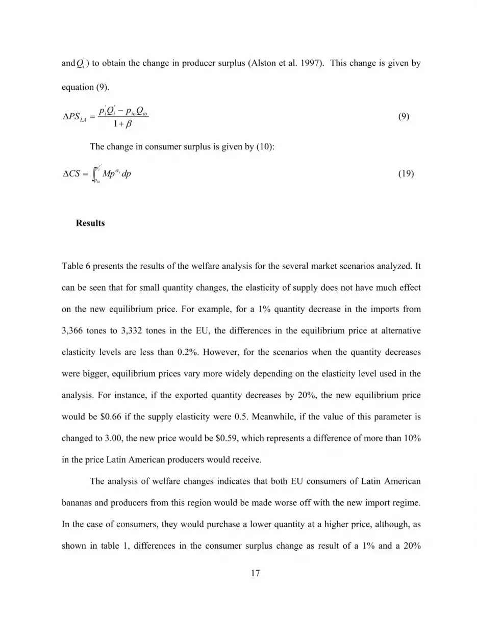
and 'iQ ) to obtain the change in producer surplus (Alston et al. 1997). This change is given by

equation (9).

β+−

=∆1

''ioioii

LAQpQp

PS (9)

The change in consumer surplus is given by (10):

∫=∆'c

i

io

ip

pdpMpCS α (19)

Results

Table 6 presents the results of the welfare analysis for the several market scenarios analyzed. It

can be seen that for small quantity changes, the elasticity of supply does not have much effect

on the new equilibrium price. For example, for a 1% quantity decrease in the imports from

3,366 tones to 3,332 tones in the EU, the differences in the equilibrium price at alternative

elasticity levels are less than 0.2%. However, for the scenarios when the quantity decreases

were bigger, equilibrium prices vary more widely depending on the elasticity level used in the

analysis. For instance, if the exported quantity decreases by 20%, the new equilibrium price

would be $0.66 if the supply elasticity were 0.5. Meanwhile, if the value of this parameter is

changed to 3.00, the new price would be $0.59, which represents a difference of more than 10%

in the price Latin American producers would receive.

The analysis of welfare changes indicates that both EU consumers of Latin American

bananas and producers from this region would be made worse off with the new import regime.

In the case of consumers, they would purchase a lower quantity at a higher price, although, as

shown in table 1, differences in the consumer surplus change as result of a 1% and a 20%

18

quantity decrease range from 12% and 23% depending on the supply elasticity. For example,

losses are of around $1,725 when the quantity imported decreases 1% from 2002 levels for an

elasticity of 1. If the quantity decrease were of 20%, those loses would rise to $2,067.

The same can not be said for producers’ welfare changes. The welfare lost for Latin

American producers would increase from $4,330 to $90,507 depending on whether quantity

decreases by 1% or 20%, respectively.

A sensitivity analysis to determine the behavior of consumer and producer surplus

changes with respect to elasticity values not only supports those findings but also gives other

interesting results. Figure 2 shows how the change in consumer surplus changes as the supply

elasticity increases. As supply becomes more elastic, the change in consumers’ surplus due to a

1% quantity decrease decreases at a decreasing rate. The same behavior is observed for any

quantity change.

In the case of producers, the degree of surplus loss from the supply being more elastic

depends on the magnitude of the elasticities. For low values, the change in welfare lost

increases as the supply becomes more elastic. However, after attaining a supply elasticity of

one, this relationship reverses and the change in producers’ surplus losses become lower as

their supply gets more elastic (note, these are changes in producer surplus, not the level of

surplus).

19

Table 6. Results from the Welfare Analysis of the EU import tariff to Latin American suppliers

Percentage change in LAT imports Latin American

supply -1.0% -3.0% -5.0% -7.5% -10.0% -15.0% -20.0% New producer price ($/kg)

0.50 0.564 0.573 0.582 0.593 0.606 0.632 0.661 1.00 0.563 0.569 0.576 0.584 0.593 0.612 0.632 2.00 0.562 0.566 0.570 0.575 0.581 0.593 0.606 3.00 0.561 0.564 0.567 0.571 0.575 0.584 0.593

New consumer price ($/kg) 0.50 0.809 0.8178 0.827 0.838 0.851 0.877 0.906 1.00 0.808 0.8143 0.821 0.829 0.838 0.857 0.877 2.00 0.807 0.8110 0.815 0.821 0.826 0.838 0.851 3.00 0.806 0.8094 0.812 0.816 0.821 0.829 0.838

Change in Consumer surplus from Latin American banana imports (2002 US$) 0.50 -1728.50 -1766.47 -1805.34 -1855.27 -1906.77 -2014.85 -2130.45 1.00 -1725.71 -1757.99 -1791.02 -1833.42 -1877.13 -1968.78 -2066.69 2.00 -1722.06 -1746.89 -1772.28 -1804.86 -1838.42 -1908.71 -1983.67 3.00 -1719.77 -1739.95 -1760.57 -1787.03 -1814.26 -1871.26 -1931.99

Change in LAT Producers surplus (2002 US$) 0.50 -4322.20 -13038.22 -21852.29 -33012.67 -44337.91 -67512.03 -91438.18 1.00 -4330.20 -13046.99 -21840.83 -32945.03 -44178.06 -67051.54 -90506.91 2.00 -3779.31 -11372.40 -19012.47 -28630.58 -38326.78 -57964.91 -77951.86 3.00 -3227.18 -9704.17 -16211.98 -24391.32 -32621.72 -49242.82 -66090.72

20

Figure 2. Change in consumer surplus at alternative supply elasticity values (Change in LA quantity=-1%)

-1755.00

-1750.00

-1745.00

-1740.00

-1735.00

-1730.00

-1725.00

-1720.00

-1715.00

0.50

0.70

0.90

1.10

1.30

1.50

1.70

2.00

2.20

2.40

2.60

2.80

3.00

3.20

3.40

3.60

3.80

4.00

4.20

4.40

4.60

Supply elasticity

Cha

nge

in C

S (2

002

US$

)

21

Figure 3. Change in producer surplus at alternative elasticity values (% change in LA quantity=-1%)

-4,600

-4,400

-4,200

-4,000

-3,800

-3,600

-3,400

-3,200

-3,000

-2,800

-2,600

0.50

0.70

0.90

1.10

1.30

1.50

1.70

2.00

2.20

2.40

2.60

2.80

3.00

3.20

3.40

3.60

3.80

4.00

4.20

4.40

4.60

Supply elasticity

Cha

nge

in P

S (2

002

US

$)

22

References

Alston, J, K. Foster and R. Gree. “Estimating elasticities with the Linear Approximate Almost

Ideal Demand System: Some Monte Carlo Results.” The Review of Economics and Statistics 76:2 (1994): 351-356

Borrell, B. and Y. Maw-Cheng. “EC Bananarama 1990.” The Developing Economies XXX-3

(1992): 259-283. Borrell, B. and Y. Maw-Cheng. “EC Bananarama 1992: The Sequeil.” The Developing

Economies XXX-3 (1992): 259-283. Borrell, B. “EC Bananarama III. Working Paper 1386, 1994. Borrell, B. “Policy Making in the EU: the bananarama story, the WTO and policy

transparency” The Australian Journal of Agricultural Economics 41:2 (1997): 263-276. Eales, J. “The Inverse Almost Ideal Demand System.” European Economic Review 38 (1994):

101-115 Hervé G., C. Loroche and C. Le Mouël. “Impacts of the Common Market Organization for

Bananas on European Union Markets, International Trade and Welfare” Journal of Policy Modeling 21(1999):619-631.

Hervé G., C. Loroche and C. Le Mouël. “An economic assessment of the Common Market

Organization for bananas in the European Union” Agricultural Economic 20 (1999):105-120.

Kox, H. “Welfare Gains from liberalized banana trade and new international banana

agreement.” Source unknown Lutz, K. “Impacts of the banana market regulation on international competition, trade and

welfare.” European Review of Agricultural Economics 22 (1955): 321-335. McCorriston, S. “Market Structure Issues and the Evaluation of the Reform of the EU Banana

Regime.” World Economy 23 (2000): 923-937. Read, R. “The EC Internal Banana Market: The Issues and the Dilemma.” World Economy 17

(1994): 219-235.