Embed Size (px)
Citation preview

MPRAMunich Personal RePEc Archive
Import Demand in Heterogeneous PanelSetting
Nasri Harb
United Arab Emirates University
2005
Online at http://mpra.ub.uni-muenchen.de/13622/MPRA Paper No. 13622, posted 26. February 2009 04:55 UTC
1
United Arab Emirates University
College of Business and Economics Department of Economics
Working Paper No. 04/05– 07
Import Demand in Heterogeneous Panel Setting*
Nasri HARB**
March 2005
*The author thanks Peter Pedroni for helpful comments. **Economics Department, UAE University, P.O. Box 17555, Al-Ain, United Arab Emirates, email: [email protected]

2
ABSTRACT To study the elasticities of import demand function, we build a heterogeneous panel
with data of 40 countries and use panel unit root tests (Im, Pesaran and Shin, 1997)
and panel cointegration tests (Pedroni, 2004). We test our model with two previously
used activity variables: GDP and GDP minus Export for a performance comparison.
To estimate our elasticities, we make use of two modified panel version of FMOLS
and DOLS developed by Pedroni (1996, 2000, 2001). Our tests prove that GDP
outperforms GDP minus Exports as an activity variable in the cointegration context.
FMOLS and DOLS give close results when we do individual estimates. When we
use between-dimension estimators, we get conflicting results. Then, we split our
sample into developed and developing countries and show that income elasticity in
developing countries are not different than unity on average and are higher than in
developed countries contradicting previous literature results.
Key words: Import Demand elasticities, Time series, Panel
cointegration, FMOLS, DOLS.
JEL Classification: C22, C23, F10.
*Economics Department, UAE University, P.O. Box 17555, Al-Ain, United Arab Emirates, email: [email protected]

3
I INTRODUCTION
Many attempts have been made to estimate the Import Demand Function (IDF,
hereafter) in different countries. The importance of this applied exercise stems from
the effect of foreign trade and trade policy on the local economy. Also, devaluation
in many countries is based on the negative effect it has on real exchange rate, which
in turn discourages imports and improves trade balance. Thus, the value of import
elasticity with respect to major macroeconomic factors reveals the degree to which
the local economy is subject to foreign countries’ disturbances and the effectiveness
of a devaluation policy.
Among the earliest papers in this field of applied research is Thursby and Thursby
(1984) where the authors estimated different specifications of the IDF for five
developed countries. They concluded that including lagged values of the dependent
variables improves the model specification. Goldstein and Khan (1985) presented a
detailed literature review on the Import and Export functions, their specifications,
estimation methodologies and the problems arising from the choice of variables and
simultaneity. Both papers however, are dated before the development of the
cointegration literature. Cointegration technique is important in the case of IDF
because of the presence of unit root in the related data series. Clarida (1994) used
these econometric advances to estimate the US import elasticity of non-durable
goods. Instead of an ad-hoc model, he estimated an IDF based on a simple rational
expectations general equilibrium model. To tackle the problem of simultaneity, he
applied a technique developed by Phillips and Loretan (1991), which consists of

4
including a lagged value of the deviation from the long run relationship. His results
showed that US income and price elasticities of imports are 2.20 and –0.94
respectively. Reinhart (1995) estimated price and income elasticities of imports for
12 developing countries with 25 observations each. Her model suggested that the
right scale variable is permanent income or a measure of wealth for which she used
GDP as a proxy. She applied a dynamic estimator proposed by Stock and Watson
(1990). Her estimates proved to be sensible. Moreover, she found evidence of
Houthakker and Magee (1969) results; that is, the developing countries' income
elasticity of imports is lower than developed countries' (which in her model are
equal to the exports of the developing countries). However, the data of some
countries in her sample did not show proper behavior in terms of cointegration.
Hence, she pooled the observations into regional blocks in order to highlight the
characteristics of each block. She found out that Houthakker and Magee (1969)
results re-emerged in Asian and Latin American countries, but not in Africa.
Senhadji (1997) used Philips and Hansen (1990) FMOLS technique to estimate the
IDF idiosyncratic parameters for a set of 77 countries. His simple model suggested
that the scale variable is GDP minus exports (GDPX). He included a lagged
adjustment term into his model as suggested by previous studies, and concluded that
the average long run income and price elasticities are 1.45 and –1.08 respectively.
The data span varied between 27 and 34 annual observations depending on the data
availability for each country.
A central point in IDF is the unitary elasticities. Reinhart's (1995) and Senhadji's
(1997) models assume that import elasticities with respect to price and income are

5
respectively equal to one and minus one respectively. This may not be true
(Reinhart, 1995) however, because of 1) the over simplified theoretical model, 2) the
noise introduced by the use of proxies, and 3) the assumption that imports consist of
final goods only, which is not too realistic.
In the context of panel studies like ours therefore, it is likely that these same factors
have varying effects across each country in the panel which strongly suggests that
the panel in our hand is heterogeneous. Accordingly, this paper calls upon recent
developments in heterogeneous panel econometrics, which have opened wide the
gate of applied research especially in developing countries where short time series
data are an important obstacle for empirical research. To overcome the heterogeneity
problem and reduce the small samples distortions, we build a heterogeneous panel to
study the characteristics of the IDF and estimate its elasticities. Specifically, after
pooling the data of 40 countries, we use the methodology proposed by Im, Pesaran,
and Shin (1997, IPS hereafter) to test for the existence of unit root in our data series
as predicted by the theory taking into account its heterogeneous characteristics in
terms of fixed effect and autocorrelation parameter. Then, we verify the null of no
cointegration hypothesis amongst our data series using Pedroni’s (2004)
cointegration tests. These tests take the heterogeneous dynamic features of the series
into account and do not constraint the cointegration vectors to be the same across the
members. Ignoring these series features will have serious effects as we are going to
see.
Other recent econometric techniques that we make use of are developed by Kao and
Chiang (1997) and Pedroni (1996, 2000). The former proposed a parametric DOLS

6
panel estimator that pools the data along the within-dimension. They showed that
this estimator has the same asymptotic distribution as the adjusted FMOLS within-
dimension panel estimator proposed by Pedroni (1996). Yet, both estimators show
relatively large distortions in small-size samples. Consequently, Pedroni (2000,
2001) showed that between-dimension (group-mean) panel FMOLS and DOLS
estimators demonstrate minor size distortions in small samples. The between-
dimension estimators have two advantages in heterogeneous panels. First, they allow
greater flexibility in hypothesis testing. Second, they provide an estimate of the
cointegrating vectors' mean. The details of those estimators are left to section (2).
Our results show that all our panel variables are non-stationary. The cointegration
analysis reveals that GDP outperforms GDPX as an activity variable. The individual
elasticities are in general conformed to the theory with few exceptions and most of
them are significantly different from unity. FMOLS and DOLS results are close to
each other. With panel estimators however, they provide contradicting results. To
further investigate the elasticities' characteristics, we split our sample into
developing and developed countries and found that income elasticities in developing
countries are equal to one on average, but unlike previous studies, are higher than
those of developed countries
The remaining of this paper is organized as follows: section (2) provides the
theoretical background, the specification of the IDF model, and discusses the
econometrical issues; section (3) presents the results of the tests and estimation
while section (4) concludes.

7
II THE MODEL AND THE METHODOLOGY
The following subsection (1) discusses the theoretical model behind our IDF. We
use a simple model developed by Reinhart (1995) and compare the equation she
used for estimation with the one used by Senhadji (1997). Even if her basic model is
not exactly the same as Senhadji's, we still can use it to compare both IDFs.
Subsection (2) discusses the econometric aspects of our paper.
1) THE THEORETICAL MODEL
We assume an infinitely lived representative rational agent in a small open economy.
At each period t, she consumes a non-traded home good ht and an imported good mt.
She has a stochastic endowment of the home good, qt, and of the export good, xt. At
each period, her total endowment (or GDP) is therefore, t
xtt p
pxq
+ where px is the
price of exports, p is the price of the home good or the numeraire, and the price ratio
t
x
pp
is the relative price of exports. She chooses quantities of the home good and
imported good that maximize an infinite utility function. In a discrete time setting,
her problem is presented as
Max
{ tt mh , }
( ) ( )( )
−+∑
∞
=0ln1)ln(
ttt
t mh ααβ (1)
subject to the following constraint:
8
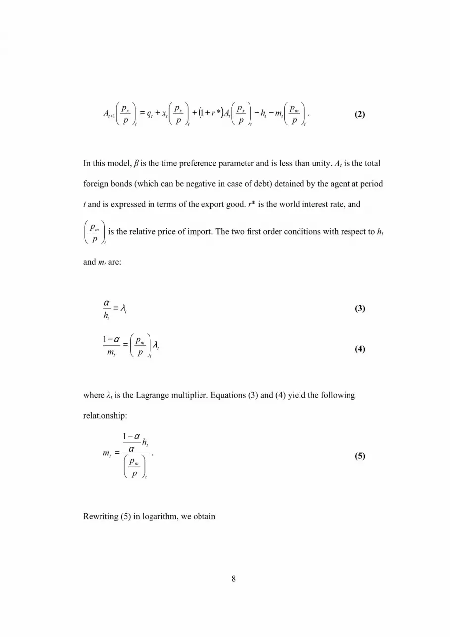
( )t
mtt
t
xt
t
xtt
t
xt p
pmhppAr
ppxq
ppA
−−
++
+=
+ *11 . (2)
In this model, β is the time preference parameter and is less than unity. At is the total
foreign bonds (which can be negative in case of debt) detained by the agent at period
t and is expressed in terms of the export good. r* is the world interest rate, and
t
m
pp
is the relative price of import. The two first order conditions with respect to ht
and mt are:
tth
λα =
tt
m
t pp
mλα
=−1
(3)
(4)
where λt is the Lagrange multiplier. Equations (3) and (4) yield the following
relationship:
t
m
t
t
pp
hm
−
= αα1
. (5)
Rewriting (5) in logarithm, we obtain

9
( ) ( )t
mtt p
phcm
−+= lnlnln (6)
where
−=
αα1lnc . Since GDP is equal to
t
xtt p
pxq
+ , and since tt hq = is a
clearing condition, it follows that
( )t
m
t
xtt p
pppxGDPcm
−
−+= lnlnln . (7)
On the other hand, since the major interest is to estimate the long run elasticities of
imports, Reinhart takes into account the steady state budget constraint, that is
( )
−−
++
+=
p
pmh
pp
Arpp
xqpp
A mxxx *1 . (8)
Rearranging (8) and taking into account the market clearing condition q=h, we
obtain
+
=p
pppAr
ppxm mxx /* . (9)
Rewriting (9) in log, we obtain

10
( ) ( )
−
+=
pp
ppArxm mx ln*lnln . (10)
Equation (10) states that, in the long run, imports have a positive relationship with
the wealth or permanent income and a negative relationship with their relative
prices. While Reinhart (1995) estimates (10) as the IDF, Senhadji (1997) uses (7).
But he added, on an ad hoc basis, a partial adjustment term as suggested by Thursby
and Thursby (1984) to add dynamics to his model.
The difference between both equations is reflected on the choice of the activity
variable. While (7) uses GDPX, (10) uses exports plus interests on net assets.
Reinhart used GDP as a proxy for wealth because of data limitations. In this paper,
we estimate IDF using both specifications of the activity variable and compare the
performance of each.
A common aspect to both models is that they predict that elasticities with respect to
the activity variable and price to be one and minus one respectively. As stated above,
this may not be true. There are many reasons to believe that those elasticities may
not be equal to one. For instance, if we use a utility function with constant elasticity
of substitution, we would have found that import elasticity will depend on the
intratemporal elasticity of substitution. Also, proxies such as GDP or relative price
of imports may introduce a measurement error which deviate those elasticities from
unity. Another argument against unit elasticity is the type of imported goods. In our
model, imports consist of final goods. In real data, imports include final and
intermediate goods and raw materials as well. It is plausible to think that those

11
factors have different effects in different countries, which leads us to assume that our
panel is heterogeneous.
2) THE ECONOMETRIC METHODOLOGY
As mentioned above, we use IPS (1997) unit root tests. Two tests have been
proposed, the LM-bar test and the t-bar test. Both allow for heterogeneity across
members and residuals serial correlation. Their null hypothesis assumes that λi=1
(where i indicates the cross sectional member) against the alternative that λi < 1 in
some or all "i"s in
tijti
p
jjitiitiiti xxx
i
,,1
,1,,, )1( υρλθµ +∆+−−+=∆ −=
− ∑ (11)
where xi,t is the time series to be tested, tix ,∆ is the first difference of xi,t and µi is the
fixed effect. θi allows for an idiosyncratic linear trend for each group while νi,t is
i.i.di. Monte Carlo experiments show that IPS (1997) tests outperform Levin and
Lin (1993) test. They have greater power and better small-sample properties.
Moreover, IPS (1997) showed that t-bar test has better performance over LM-bar
test when N and T are small.
While the same unit root test can be applied for both raw and residuals data in
conventional time series with proper adjustments to the critical values when applied
to residuals, Pedroni (2004) observed that testing for residuals' unit root in panel data
is not so straightforward. He proved that if the regressors are not strictly exogenous
and if the cointegrating relationship is not constrained to be homogeneous across
members, then proper adjustments should be made to the test statistics themselves.

12
Otherwise, the test becomes divergent asymptotically; that is, as the sample size
grows large, one is certain to reject the null of no cointegration regardless of the true
relationship. Moreover, he showed that imposing homogeneity falsely across
members generates an integrated component in the residuals making them non-
stationary leading an econometrician to conclude that her variables are not
cointegrated even if they truly are.
For these reasons, he defines two sets of statistics. The first one consists of three
statisticsNTNTNT tZZZ and ,
1ˆˆ −ρν. These statistics are based on pooling the residuals
along the within-dimension of the panel. They are respectively analogous to the
“panel variance ratio”, “panel rho”, and “panel t” statistics in Phillips and Ouliaris
(1990).
The second set of statistics NTNT tZZ ~,~
1ˆ −ρ is based on pooling the residuals along the
between-dimension of the panel. The basic of both statistics is to compute the group-
mean of the individual conventional time series statisticsii. The asymptotic
distribution of each of those five statistics can be expressed in the following form:
)1,0(, NNX TN ⇒
−
νµ
(12)
where XN,T is the corresponding form of the test statistic, while µ and ν are the mean
and variance of each test respectively. They are given in table (2) in Pedroni (1999).
Under the alternative hypothesis, Panel ν statistic diverges to positive infinity.
Therefore, it is a one sided test were large positive values reject the null of no
cointegration. The remaining statistics diverge to negative infinity, which means that
large negative values reject the null.
13
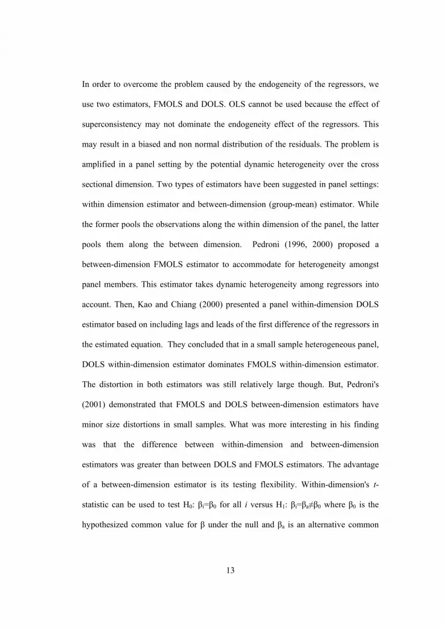
In order to overcome the problem caused by the endogeneity of the regressors, we
use two estimators, FMOLS and DOLS. OLS cannot be used because the effect of
superconsistency may not dominate the endogeneity effect of the regressors. This
may result in a biased and non normal distribution of the residuals. The problem is
amplified in a panel setting by the potential dynamic heterogeneity over the cross
sectional dimension. Two types of estimators have been suggested in panel settings:
within dimension estimator and between-dimension (group-mean) estimator. While
the former pools the observations along the within dimension of the panel, the latter
pools them along the between dimension. Pedroni (1996, 2000) proposed a
between-dimension FMOLS estimator to accommodate for heterogeneity amongst
panel members. This estimator takes dynamic heterogeneity among regressors into
account. Then, Kao and Chiang (2000) presented a panel within-dimension DOLS
estimator based on including lags and leads of the first difference of the regressors in
the estimated equation. They concluded that in a small sample heterogeneous panel,
DOLS within-dimension estimator dominates FMOLS within-dimension estimator.
The distortion in both estimators was still relatively large though. But, Pedroni's
(2001) demonstrated that FMOLS and DOLS between-dimension estimators have
minor size distortions in small samples. What was more interesting in his finding
was that the difference between within-dimension and between-dimension
estimators was greater than between DOLS and FMOLS estimators. The advantage
of a between-dimension estimator is its testing flexibility. Within-dimension's t-
statistic can be used to test H0: βi=β0 for all i versus H1: βi=βa≠β0 where β0 is the
hypothesized common value for β under the null and βa is an alternative common

14
value. But, the group-mean estimator allows to test H0: βi=β0 for all i versus H1:
βi≠β0 for all i, so that the value of β is not necessarily constrained to be the same
across the members under H1. Two more advantages are cited in favor of between-
dimension estimator: 1) when the true cointegrating vectors are heterogeneous, it
provides the mean value of the cointegrating vectors while the within-dimension
estimator provides the average regression coefficient, and 2) its t-statistic exhibits
relatively little distortions in small samples (Pedroni, 2000). We use both estimators
in our article for the sake of comparison.
III RESULTS
We got the data from IFS and UNCDB. The data starts at a different year in each
country depending of its availability. We choose to use 28 years of observations in
each country in order to maximize the cross sectional dimension of our panel to 40.
Nominal GDP, imports and exports are deflated using consumer price index. We
divide the unit value of imports by consumer price index to obtain relative price of
imports as in Reinhart (1995). Lag truncation has been set to a maximum of two for
all tests and kernels because we have annual data. We start by testing for the
existence of unit root in all our variables using both IPS tests: t-test and LM-bar test.
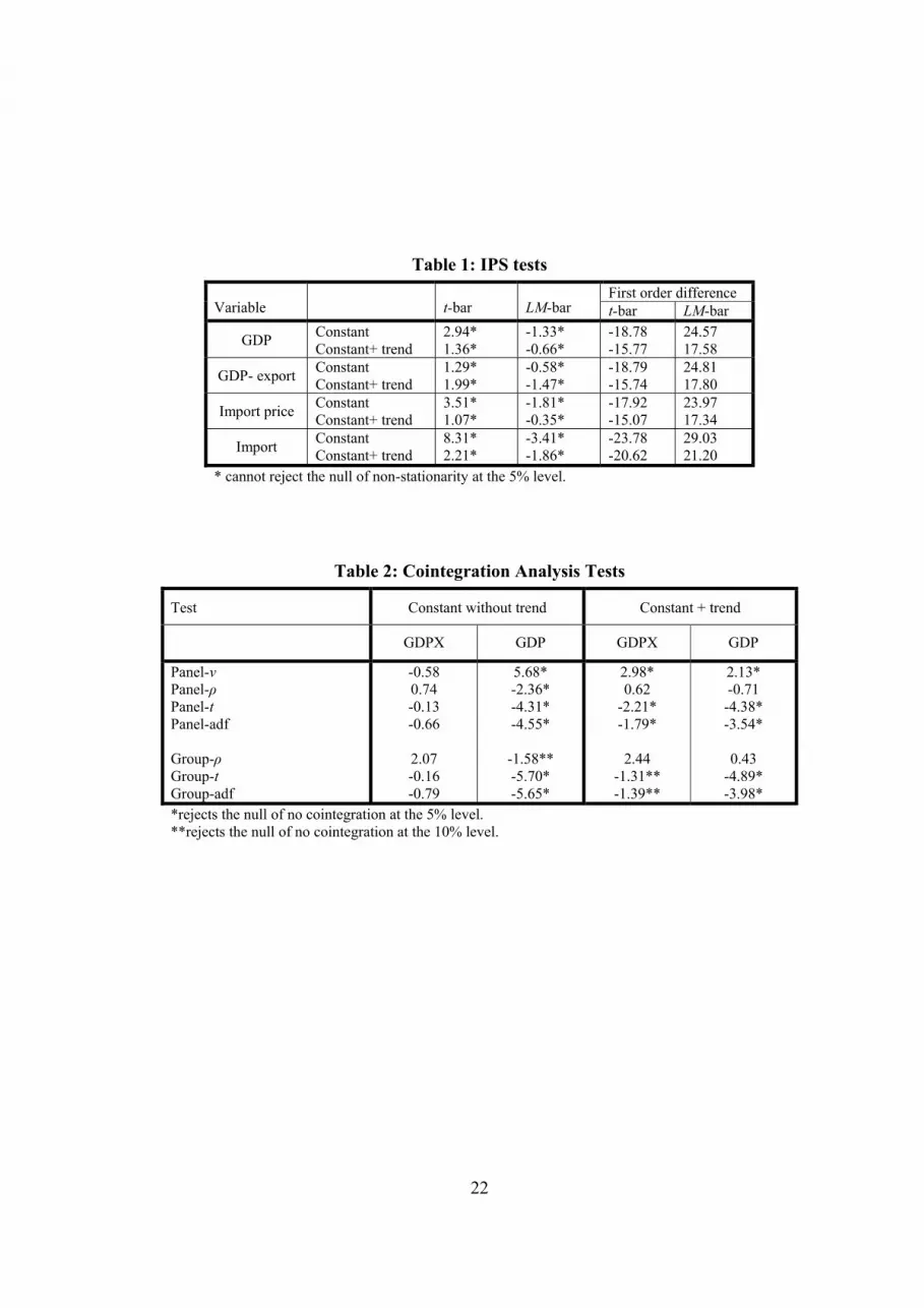
It is clear from table (1) that the four aggregates have unit root using either tests.
Moreover, when the tests are applied to the first order differences, the null of non-
stationarity is easily rejected indicating that our four variables are I(1).
Cointegration tests results using either scale variables, GDPX and GDP are shown in
table (2). The panel-adf and group-adf tests are shown for comparison only. We find

15
evidence of cointegration with both scale variables. With GDPX, the three variables
show some evidence of cointegration when we include a trend only. With GDP, we
find more evidence of cointegration when a trend is excluded. Since ν and ρ tests
tend to under-reject the null of no cointegration (Pedroni, 2004), we can conclude
that there is a strong evidence of cointegration amongst our variables using both
aggregates.
The normal next step would be to estimate the cointegrating vectors. A problem
arises here consisting on whether to estimate the cointegrating vectors with or
without the deterministic trend. So far, no test has been developed to verify the
significance of the heterogeneous deterministic trend in panel estimation. Moreover
and to our knowledge, all previous work on import demand function estimation have
not included a deterministic trend in the cointegration vector. Therefore, and in order
to keep in the same line of previous research, we estimate our model with no
deterministic trend. This allows us an easier comparison with other results. This
decision will make us discard GDPX as the activity variable at this stageiii. Another
motivation to estimate with no deterministic trend is that, in the case of GDP with no
trend, all our tests reject the null of no cointegration which suggests a better
performance.
We pursue our analysis therefore, and estimate the idiosyncratic cointegration
vectors using FMOLS and DOLS followed by the panel cointegration vector. We
test H0: income elasticity of imports = 1 and H0: price elasticity of imports = -1.
Results are shown in table (3) where the numbers in parenthesis are the t tests.

16
The elasticities with respect to income are close to each other using either FMOLS
or DOLS. Using FMOLS (DOLS), 29 countries (31 countries) out of 40 show long
run positive income elasticities significantly different from unity. They range
between 0.40 (Kenya and Norway) and 2.77 (New Zealand, Spain and US). This
compares to a wider range in Senhadji (1997) where the significant estimates ranged
between 0.34 and 5.48. This can be explained by different methodologies of
estimation and different data sets.
Regarding relative price, our estimates are negative, but significantly different from
minus one in 28 countries using FMOLS (23 countries using DOLS). They range
between -0.02 (Germany) and -2.08 (Mauritius). Again, this range is considerably
narrower than the results of Senhadji (1997) where the price elasticities ranged
between -0.01 and -6.66.
Even if we observe the large rejection rate of the null of a unitary elasticity, these
results may not be too conclusive because of the short spanned data in each country.
The last two rows to the right side in table (3) show the results of the panel estimates
which are conformed to the theory. Using the within-dimension estimator, we reject
the two null hypothesis using either FMOLS or DOLS. But as mentioned previously,
the regression on the pooled panel gives the average regression coefficients and has
therefore no economic meaning. The FMOLS and DOLS between-dimension
estimators -the average of the cointegrating vectors- with their t-statistics are
presented in the last row of table (3). They give conflicting results. While the DOLS
estimator rejects the null of unitary elasticity, FMOLS does not. Both estimators
exhibit minor distortions in small samples which mean that we cannot favor one

17
result over the other. On the other hand, both cases show that price elasticities are
significantly different from the unity.
In order to deepen our investigation and find a clearer answer to our task, we use the
United Nations classification to split our sample into two categories, developed and
developing countries. To compare between both groups, we use our heterogeneous
panel setting. The developed countries (19 countries) are indicated by the shaded
rows in table (3) while the remaining ones (21 countries) are the developing
countries. We have tried to include Cyprus and Israel in the developed countries
because they have higher per capita GDP than some developed countries. We
observed no difference in our results.
Testing different data series of developing and developed countries shows (table 4)
that they are all I(1). Turning to cointegration analysis in table (5), it is obvious that
developed and developing countries show contradicting (still weak though)
regarding the cointegration using GDPX. Since GDP demonstrates better
cointegration condition with no deterministic trend, we show the corresponding
panel cointegrating vectors in table (6) where some interesting results emerge. Using
within-dimension in both groups of countries, the income elasticity is significantly
greater than one. Also, income elasticity in developed countries (1.69, FMOLS; and
1.72, DOLS) are obviously higher than in developing countries (1.07, both FMOLS
and DOLS). These outcomes reflect Houthakker and Magee (1969) results and are in
accordance with Reinhart (1995) results. But unlike the between-dimension
estimator, these results cannot be interpreted as the average of the cointegrating
vectors but as the average regression. The between-dimension estimator shows that

18
the average income elasticity in developed countries is not significantly different
from the unity, and is higher than in developing countries'. This means, that as
income increases, balance of payments in developing countries deteriorates while the
reverse occurs in developing countries contradicting previous results.
On the other hand, table (6) shows that price elasticity is higher (in absolute values)
in developing than in developed countries and is significantly different than minus
one. This might be explained by the fact that a larger share of developed countries
import consists of raw materials while those of developing countries consist of a
larger variety of goods.

19
IV CONCLUSION
Our estimation methodology for the import demand function allows for
heterogeneity across members. Our results reveal that 1) GDP shows better
performance than GDP minus Exports and 2) income and price elasticities in
developing countries are higher (in absolute values) than in developed countries.
Our results invite international economists to investigate the difference observed in
both groups. That is, why the average elasticity is equal to unity and is higher in
developing countries than in developed countries?
Appendix
The following list shows the period covered by the data for each country in our
panel.
Australia 1972-1999 Burkina-Faso 1969-1996 Canada 1972-1999 Chile 1969-1996 Columbia 1972-1999 Costa-Rica 1966-1993 Cyprus 1960-1987 Denmark 1972-1999 Finland 1970-1997 France 1971-1999 Germany 1972-1999 Greece 1970-1997 Iceland 1970-1997 India 1971-1998 Ireland 1971-1998 Israel 1972-1999 Italy 1971-1998 Japan 1972-1999 Jordan 1971-1998 Kenya 1971-1998
Korea 1972-1999 Malaysia 1960-1987 Malta 1962-1989 Mauritius 1971-1998 Morocco 1972-1999 Netherlands 1971-1998 New Zealand 1971-1998 Norway 1972-1999 Pakistan 1972-1999 Philippines 1964-1991 Portugal 1965-1992 S. Africa 1969-1996 Spain 1971-1998 Sri Lanka 1970-1997 Sweden 1972-1999 Syria 1970-1997 Thailand 1972-1999 UK 1972-1999 USA 1972-1999 Venezuela 1971-1998

20
Acknowledgements
The author thanks Peter Pedroni for helpful comments.
Bibliography: Clarida, R. (1994) Cointegration, Aggregate Consumption, and the Demand for Imports: A Structural Econometric Investigation, The American Economic Review, vol. 84, No. 1, pp.298-308. Dutta, D., and Ahmed, N. (2001) An Aggregate Import Demand Function for India: A Cointegration Analysis, Internal Working Paper, the University of Sydney. Dutta, D., and Ahmed, N. (2001) An Aggregate Import Demand Function for India: A Cointegration Analysis, Internal Working Paper, the University of Sydney. Goldstein, M. and Khan, M. (1985) Income and Price Effect in Foreign Trade, in R. Jones and P. Kenen, EDS, Handbook of International Economics, Amsterdam, North-Holland, 1042-1099. Houthakker, H. S. and Magee, S. P. (1969): Income and Price Elasticities in World Trade, Review of Economics and Statistics, vol. 51, pp. 11-125. Im, K., Pesaran, H. and Shin, Y. (1997): Testing for Unit Roots in Heterogeneous Panels, University of Cambridge, DAE Working Paper, No. 9526.
Kao, C., and Chiang, M. (2000): On the Estimation and Inference of a Cointegrated Regression in Panel Data, Advances in Econometrics, vol. 15, pp. 179 -222. Pedroni, P. (1999): Critical Values for Cointegration Tests in Heterogeneous Panels with Multiple Regressors, Oxford Bulletin of Economics and Statistics, vol. 61, No. 4, 653-670. Pedroni, P. (1996): Fully Modified OLS for Heterogeneous Cointegrated Panels and The Case of Purchasing Power Parity, Indiana University Working Papers in Economics, No. 96-020. Pedroni, P. (2000): Fully Modified OLS for Heterogeneous Cointegrated Panels, Advances in Econometrics, vol. 15, pp. 93-130. Pedroni, P. (2001): Purchasing Power Parity Tests in Cointegrated Panels, The Review of Economics and Statistics, vol. 83, No. 4, pp. 727-731.

21
Pedroni, P. (2004): Panel Cointegration: Asymptotic and Finite Sample Properties of Pooled Time Series Tests with an Application to the PPP Hypothesis, Econometric Theory, vol. 20, No. 3, pp. 597-627. Philips, P. and Hansen, B. (1990) Statistical Inference in Instrumental Variables Regression with I(1) Processes, Review of Economic Studies, No. 57, pp. 99-125. Phillips, P. and Loretan, M. (1991) Estimating Long-Run Economic Equilibria, Review of Economic Studies, vol. 58, No. 3, pp. 407-436. Phillips, P. and Moon, H. (1999) Linear Regression Limit Theory for Nonstationary Panel Data, Econometrica, vol. 67, No. 5, pp. 1057-1111. Reinhart, C. (1995) Devaluation, Relative Prices, and International Trade: Evidence from Developing Countries, IMF Staff Papers, vol. 42, No. 2. Senhadji, A. (1997) Time-Series Estimation of Structural Import Demand Equations: A Cross-Country Analysis, IMF Working Paper, WP/97/132. Stock, J. and Watson, M. (1988) Testing for Common Trends, Journal of the American Statistical Association, No. 83, pp. 1097-1107. Stock, J. and Watson, M. (1990) A Simple MLE of Cointegrating Vectors in Higher Order Integrated Systems, NBER Technical Working Paper, No. 83. Thursby, J. and Thursby, M. (1984) How Reliable Are Simple, Single Equation Specifications of Import Demand? The Review of Economics and Statistics, Vol. 66, No. 1, pp.120-128
22
Table 1: IPS tests
First order difference Variable
t-bar LM-bar t-bar LM-bar
GDP Constant Constant+ trend
2.94* 1.36*
-1.33* -0.66*
-18.78 -15.77
24.57 17.58
GDP- export Constant Constant+ trend
1.29* 1.99*
-0.58* -1.47*
-18.79 -15.74
24.81 17.80
Import price Constant Constant+ trend
3.51* 1.07*
-1.81* -0.35*
-17.92 -15.07
23.97 17.34
Import Constant Constant+ trend
8.31* 2.21*
-3.41* -1.86*
-23.78 -20.62
29.03 21.20
* cannot reject the null of non-stationarity at the 5% level.
Table 2: Cointegration Analysis Tests
Test Constant without trend Constant + trend
GDPX GDP GDPX GDP
Panel-ν Panel-ρ Panel-t Panel-adf Group-ρ Group-t Group-adf
-0.58 0.74 -0.13 -0.66
2.07 -0.16 -0.79
5.68* -2.36* -4.31* -4.55*
-1.58** -5.70* -5.65*
2.98* 0.62
-2.21* -1.79*
2.44
-1.31** -1.39**
2.13* -0.71
-4.38* -3.54*
0.43
-4.89* -3.98*
*rejects the null of no cointegration at the 5% level. **rejects the null of no cointegration at the 10% level.

23
Table 3: Elasticities' Estimates
Elasticity with respect to Elasticity with respect to activity variable Relative Price activity variable Relative Price Country
FMOLS DOLS FMOLS DOLS Country
FMOLS DOLS FMOLS DOLS
Australia 1.54* (12.7)
1.83* (16.6)
-0.73* (3.5)
-0.37* (10.3) Malaysia 1.05
(0.65) 0.78* (-2.8)
-0.44** (1.91)
0.43* (5.0)
Burkina-Faso
0.64* (-2.1)
0.51* (-2.9)
-0.18** (1.7)
0.16 (1.1) Malta 0.97
(-0.5) 1.16* (4.3)
-0.53* (3.7)
-0.94 (0.8)
Canada 2.01* (5.46)
2.14* (13.0)
-1.02 (-0.1)
-0.87 (1.1) Mauritius 1.19*
(3.9) 0.96 (-0.2)
-1.02 (-0.09)
-2.08 (-1.2)
Chile 0.85 (-0.8)
1.12 (0.3)
-1.90* (-4.6)
-1.21 (-0.6) Morocco 0.79*
(-2.0) 0.66* (-5.8)
-1.03 (-0.2)
-1.23 (-
1.57)
Columbia 1.08 (0.91)
1.07 (1.55)
-1.59* (-4.2)
-1.68* (-5.8) Netherlands 1.49*
(8.8) 1.66* (15.8)
-0.29* (12.6)
-0.12* (19.4)
Costa Rica 1.15 (1.2)
1.38* (3.6)
-0.99 (0.2)
-0.90* (3.0)
New Zealand
2.77* (5.0)
2.76* (7.2)
-0.36* (4.9)
-0.26* (11.2)
Cyprus 1.23* (6.2)
1.20* (12.4)
0.20* (7.6)
0.40* (29.0) Norway 0.40*
(-3.2) -0.10* (-2.8)
-1.08 (-0.4)
-1.40 (-1.3)
Denmark 1.90* (6.4)
1.99* (12.4)
-0.26* (7.1)
-0.24* (15.2) Pakistan 1.02
(0.3) 1.12
(1.29) -0.78* (2.2)
-1.25 (-0.8)
Finland 1.23* (2.7)
1.22* (4.1)
-0.33* (4.8)
-0.39* (8.9) Philippines 1.80*
(6.0) 2.15* (3.5)
-1.20 (1.2)
-1.76* (-2.1)
France 2.04* (11.6)
2.48* (14.7)
-0.16* (9.7)
0.21 (16.1) Portugal 2.27*
(6.1) 2.55* (10.0)
0.07* (4.8)
0.40* (6.9)
Germany 1.51* (3.4)
1.47* (4.1)
-0.02* (4.7)
0.06* (7.2) S. Africa 0.58*
(-3.1) 0.75** (-1.85)
-0.61* (2.2)
-0.47* (4.4)
Greece 1.63* (3.9)
1.39 (1.52)
-0.56* (3.8)
-0.57* (3.7) Spain 2.77*
(7.7) 2.40* (11.1)
-0.31* (4.9)
-0.53* (6.1)
Iceland 0.74* (-4.5)
0.82* (-2.6)
-0.33* (3.0)
-0.43* (2.2) Sri Lanka 1.07
(0.7) 1.31* (2.7)
-0.70* (3.2)
-0.79* (2.10)
India 1.51* (-4.5)
1.45* (5.5)
-0.47* (3.7)
-0.34* (2.6) Sweden 1.66*
(4.9) 1.70* (12.0)
-0.50* (3.9)
-0.44* (11.1)
Ireland 1.56* (16.5)
1.58* (11.0)
-0.04* (13.5)
0.02* (12.3) Syria 1.34**
(1.87) 1.06
(0.33) -1.08 (-1.3)
-1.14* (-2.9)
Israel 0.82 (-1.4)
1.07 (1.1)
-0.98** (1.79)
-0.94* (10.2) Thailand 1.47*
(9.37) 1.45* (12.3)
-0.75 (1.1)
-0.77 (0.6)
Italy 1.22* (2.8)
1.38* (4.1)
-0.49* (5.8)
-0.37* (11.1) UK 1.79*
(4.3) 1.48** (1.89)
-0.25* (4.2)
-0.58** (1.66)
Japan 1.30 (1.0)
1.12** (1.95)
-0.37* (4.1)
-0.45* (16.0) USA 2.28*
(16.6) 2.77* (8.54)
-0.30* (7.6)
0.31* (5.8)
Jordan 1.37* (2.8)
1.29* (2.6)
-0.36* (2.1)
-0.87 (0.4) Venezuela 1.06
(0.2) 0.48 (-0.8)
-0.52 (1.3)
-0.30 (1.17)
Kenya 0.50* (-2.4)
0.40* (-5.6)
-1.14 (-0.8)
-1.37* (-5.3)
Within Dimension
1.37* (-22.5)
1.38* (27.9)
-0.60* (19.7)
-0.59* (33.0)
S. Korea 1.08 (0.8)
1.0 (0.2)
-0.51** (1.7)
-0.57* (3.5)
Between Dimension
1.06 (1.37)
1.20* (4.8)
-0.72* (14.9)
-0.81* (15.9)
*reject the null with 95% significance level. ** reject the null with 90% significance level.

24
Table 4: IPS tests-Developed & Developing countries
First order difference
Variable t-bar LM-bar
t-bar LM-bar
GDP Constant Constant+ trend
3.80* 0.33*
-1.10* 0.57*
-12.09 -9.67
15.94 11.03
GDP- export
Constant Constant+ trend
0.98* 0.58*
-0.20* -0.41*
-12.26 -9.69
16.17 11.08
Import price Constant Constant+ trend
4.00* -1.46*
-2.91* 1.82**
-13.10 -11.69
17.27 13.11
DEVELOPED
COUNTRIES
Import Constant Constant+ trend
8.16* 1.39*
-3.70* -1.10*
-16.36 -14.88
20.76 15.74
GDP Constant Constant+ trend
1.20* 1.56*
-0.80* -1.45*
-30.37 -28.00
33.20 24.94
GDP- export
Constant Constant+ trend
0.84* 2.20*
-0.61* -1.64*
-14.48 -12.78
18.66 13.86
Import price Constant Constant+ trend
1.03* 2.86*
0.27* -2.22*
-11.84 -10.61
15.58 11.93
DEVELOPING
COUNTRIES
Import Constant Constant+ trend
3.70* 1.73*
-1.19* -1.52*
-14.73 14.14
19.14 14.14
* cannot reject the null of non-stationarity at the 5% level
Table 5: Cointegration Analysis Tests-Developed & Developing countries
No trend Constant + trend Test
GDPX GDP GDPX GDP
DEVELOPED COUNTRIES
Panel-ν Panel-ρ Panel-t Panel-adf Group-ρ Group-t Group-adf
-1.05 1.09 0.94 0.29 2.21 1.60 1.08
4.02* -2.22* -3.25* -2.51* -1.72* -4.11* -2.85*
3.32* -0.33 -1.80* -1.09
1.19 -0.84 -0.66
1.58** -0.81
-3.00* -1.86*
-0.29
-3.78* -2.36*
DEVELOPING COUNTRIES
Panel-ν Panel-ρ Panel-t Panel-adf Group-ρ Group-t Group-adf
0.42 -0.22 -1.39** -1.42** 0.76 -1.74* -2.12*
3.70* -1.57** -3.33* -3.63* -0.65 -4.04* -4.48*
1.21 1.01
-1.44** -1.50**
2.23 -1.01
-1.29**
1.44** -0.21
-3.21* -3.11*
0.88
-3.17* -3.25*
*(**) rejects the null of no cointegration at the 5% (10%) level.

25
Table 6: Developed and Developing Countries'
Elasticities (no trend) GDP Relative Price FMOLS DOLS FMOLS DOLS Developed
Within Dimension 1.69* (25.71)
1.72* (33.18)
-0.39* (23.52)
-0.32* (37.87)
Between Dimension 0.75* (-2.56)
0.67* (-4.88)
-0.42* (15.57)
-0.48* (13.97)
Developing
Within Dimension 1.07* (6.52)
1.07* (6.95)
-0.79* (4.81)
-0.84* (9.49)
Between Dimension 1.04 (-1.09)
1.23 (-1.18)
-0.94* (5.47)
-0.92* (8.03)
The author thanks Peter Pedroni for helpful comments. i IPS (1997) presented a modified test to allow for serially correlated disturbances as well. ii A group-mean variance ratio statistics is not presented because it is dominated by the two other statistics. iii The estimation results of the corresponding cointegrating vectors are available from the author upon request.