Embed Size (px)
Citation preview

INEQUALITY AND THE US IMPORT DEMAND FUNCTION
MARGARITA KATSIMI THOMAS MOUTOS
CESIFO WORKING PAPER NO. 1827
CATEGORY 6: MONETARY POLICY AND INTERNATIONAL FINANCE OCTOBER 2006
An electronic version of the paper may be downloaded • from the SSRN website: www.SSRN.com • from the RePEc website: www.RePEc.org
• from the CESifo website: Twww.CESifo-group.deT

CESifo Working Paper No. 1827
INEQUALITY AND THE US IMPORT DEMAND FUNCTION
Abstract In this paper we build a model of trade in vertically differentiated products and find that income inequality can affect the demand for imports even in the presence of homothetic preferences. The empirical importance of changes in inequality on the demand for imports is then assessed by examining US data for the 1948-1996 period. Using the Johansen (1988) procedure we find that there is no evidence of a long run relationship of a standard imports equation (one including imports, income, and relative prices). However, once we include a measure of inequality in our VAR specification we find not only evidence for the existence of a cointegrating equation in imports, income, relative prices and inequality, but that the evolution of inequality has a large and positive influence on the demand for imports in the US. Moreover we find that our results are robust to alternative methods of estimating cointegration equations.
JEL Code: F13, H23, O24.
Keywords: inequality, US import demand, vertically differentiated products, cointegration.
Margarita Katsimi Athens University of Economics and
Business Department of International and European
Economic Studies Patission 76 Athens 10434
Greece [email protected]
Thomas Moutos Athens University of Economics and
Business Department of International and European
Economic Studies Patission 76 Athens 10434
Greece [email protected]
July, 2006 We wish to thank to Menzie Chinn, Jaime Marquez, Nikitas Pittis and Ekaterini Panopoulou for many helpful comments and suggestions.

1 Introduction
Standard speci�cations of import demand functions are usually based on the imperfect sub-
stitutes model, in which imports and domestically produced goods are not perfect substitutes
(see, for example, Armington (1969), Goldstein and Khan (1985), Rose (1991), Hooper and
Marquez (1995)). In this model, the demand for imports is usually thought of as the result
of a representative household�s maximization of utility (which depends on the consumption
of a�domestic� and an �imported� good) subject to a budget constraint.1 The(aggregate)
volume of imports is thus speci�ed as an increasing function of aggregate income and of the
ratio of domestic to imported goods prices.Implicit in this derivation of the import demand
function is the idea that the distribution of income is not an important determinant of the
demand for imports.
In the present paper we examine the -ceteris paribus- e¤ects of changes in income in-
equality on the demand for imports.2 We do this by using a model of trade in vertically-
di¤erentiated products in which household income determines the quality of goods demanded
(Linder (1961), Flam and Helpman (1987)).3 The domestic country is assumed to have
1 In the case that the imported goods are intermediates used in domestic production, the demand forimports arises from pro�t maximization and it depends on relative prices and gross domestic product (e.g.,Kohli (1982)).
2 Although the in�uence of income inequality on macroeconomic outcomes has not been an active area ofresearch in the �eld of open-economy macroeconomics, the same does not hold true for the �eld of internationaltrade. Indeed, there is a large theoretical and empirical literature examining the e¤ects of inequality on tradepatterns in the presence of non-homothetic preferences (e.g. Markusen (1986), Hunter (1991), Francois andKaplan (1996), Mitra and Trindade (2003). In addition to its focus, the present paper di¤ers from thisliterature in that we examine the e¤ects of inequality in a model with homothetic preferences in the presenceof vertically di¤erentiated products.
3 Schott (2003) presents evidence that testi�es to the importance of vertical intra-industry trade in theworld economy. He �nds that "... the relationship between unit values, exporter endowments and exporterproduction techniques supports the view that capital- and skill-abundant countries use their endowmentadvantage to produce vertically superior varieties, i.e. varieties that are relatively capital or skill intensiveand possess added features or higher quality, thereby commanding a relatively high price" (Schott (2003),
1

comparative advantage and to export to the rest of the world (ROW)), high-quality (and
high-price) varieties of the di¤erentiated product, whereas it imports low-quality (and low-
price) varieties that are consumed by low-income households. We show that mean-preserving
changes in income inequality have an ambiguous e¤ect on the demand for imports.
The �avour of the argument can be understood by the example of a hypothetical mean-
preserving increase in income inequality. Let there be an income level such that all households
with income up to this level (call it �) maximize their utility (which depends on the quality
of the vertically-di¤erentiated product and the quantity of a homogeneous non-traded good)
by purchasing low-quality, low-price imported varieties; similarly, households with incomes
greater than � consume the high-quality domestically produced varieties. Consider now a
case in which the income of some households which intially had incomes greater than � drops
to a level below �, whereas the incomes of some households (which initially were far greater
than �) rise further, so that the average income remains intact. The e¤ect of these changes
will be an increase in imports since the households for which income has dropped below
� will switch their demand to imported varieties, whereas the households whose incomes
have increased will continue to consume domestically-produced varieties.4 We trust that the
reader will have by now thought of counterexamples in which a mean-preserving increase in
inequality results in a reduction in the demand for imports - thus intuitively con�rming the
p.658). Thus, along with Bowen et al. (1987) and Tre�er (1995) he concludes that there is no evidence ofendowment-driven specialization across products. Moreover, Grossman (1982) has attributed a signi�cantrole to vertical product di¤erentiation regarding the size and interpretation of estimated price and incomeelasticities in international trade.
4 The conclusion we draw from this example would remain intact had we assumed that, in addition to theincome changes mentioned earlier, the income of low-income households declined as well. Some readers mayregard the hypothetical changes in household incomes speci�ed in this example as a rough approximation ofthe actual changes in the US income ditribution since the mid-seventies. (see, Acemoglu (2002) for a reviewof the evidence).
2

ambiguous e¤ect of inequality on the demand for imports.
The theoretical ambiguity as to the e¤ect of income inequality on the demand for imports
is by no means an artifact of our assumption that the domestic country has comparative ad-
vantage in the production of high-quality varieties. Indeed, as section 2 of the paper makes
clear, it would also be a feature of the model if the domestic country had comparative ad-
vantage in the production of low quality varieties. This further implies that the theoretical
ambiguity would also be present if, as is the case for any country in the world in a multi-
commodity setting, the domestic country�s comparative advantage was in high-quality vari-
eties for only a sub-set of the di¤erentiated products, or if international trade was conducted
in both homogeneous and di¤erentiated goods.
In the empirical section of the paper we try to ascertain the in�uence of changes in
income inequality on the demand for US imports. For this purpose, we investigate the
existence of a long run relationship between real imports, real income, relative prices and
inequality for the 1948-1996 period. Using the Johansen (1988) procedure, we fail to detect
evidence of a standard imports equation (one including imports, income and relative prices)
The picture changes when we include a measure of inequality in our VAR speci�cation. In
fact both the trace test and the maximim eigenvalue statistic support the existence of a
cointegrating vector including imports, income, relative prices and inequality.5 We also
�nd our results to be robust to alternative methods of estimating cointegration equations,
with all methods producing remarakably similar estimates of the cointegrating vector and
5 Our �nding about the importance of income heterogeneity in explaining the behavior of United Statesimports can be considered as complementary to the one advanced by Marquez (2000) in his e¤ort to "solve"the Houthakker and Magee (1969) puzzle about the high income elasticity of US imports. Marquez argued(and provided the relevant evidence) that if immigrants retain their tastes for their native products, then anincrease in immigration would increase the demand for imports.
3

providing estimates of the elasticity of imports with respect to inequality ranging from 0.8-
1.2. Moreover, given that the e¢ ciency of the various methods in small samples may di¤er
considerably, we perform a small Monte Carlo experiment in order to assess their relative
performance in small samples. We conclude that the Johansen procedure along with the
Fully Modi�ed Least Squares estimator of Phillips and Hansen (1990) seem to perform best
both in terms of bias and variation. Interestingly, these two methods deliver the highest
estimates of the inequality elasticity.
Our estimates suggest a signi�cant impact of inequality on real imports. For example,
according to our range of estimates (0.8-1.2), had inequality in the US remained at its 1975
level, imports in 1996 would have been lower between 12 and 19 percent of the �tted value
(which is close to the actual value). The further rise in inequality since 1996 implies that
had inequality in 2004 been at its 1975 level, the percentage decline in US imports in 2004
would have been even larger than in 1996, thus implying a very large improvement in the
US current account de�cit.6
The remainder of the paper is as follows: Section 2 develops the theoretical model showing
the in�uence of income inequality on the demand for imports. The empirical analysis is
presented and discussed in section 3. The last section concludes.
2 The model
We present a simple theoretical framework capable of illustrating the in�uence of income
inequality on the demand for imports. The framework is akin to Katsimi and Moutos (2005),
6 Although recent data on US income inequality exist, in our empirical analysis we use the longer data setavailable, which covers the 1944-1996 period.
4

which has in turn borrowed from Malley and Moutos(2002) and Flam and Helpman (1987).
We will assume the existence of a small open economy, which produces (and consumes) two
goods: a homogeneous non-traded good (X) and a vertically-di¤erentiated product (Y ) that
is traded with the rest of the word (ROW). The model features two-way international trade
in the vertically-di¤erentiated good, with the domestic country producing (and exporting) a
high-quality quality variety of good Y; and importing a low-quality variety of it.
2.1 Firms
Good X (the non-traded good) is a homogeneous good produced under perfectly competitive
conditions in the domestic country with the use of labour services (L). We conceive of L
as being the simple aggregate of e¤ective labour services provided by perfectly substitutable
workers with each of them possessing di¤erent units of e¤ective labour.7 We assume that
�rms pay the same wage rate per e¤ective unit of labour - thus the distribution of talent
across �rms does not a¤ect unit production costs. For simplicity, we assume that each unit
of L produces one unit of the homogeneous good.under linear technology,
X = L (1)
Using labour as the numeraire, we get that the price of the homogeneous, non-traded good is,
PX = 1: We assume that all prices in the domestic economy and in the ROW are expressed
in a common currency (the exchange rate is �xed at unity).
7 Alternatively, we could conceive of L as a function of the quantities of labour provided by imperfectlysubstitutable groups of workers, e.g., L = f(LS ; LU ), where LS and LU stand for the e¤ective units of skilledand unskilled labour. Under the interpretation adopted in the text, changes in (income) inequality can be theresult of changes in the e¤ective number of labour units each worker (cum household) is endowed with. Underthe skilled-unskilled workers interpretation, changes in inequality can be the result of changes in the relativewage of skilled workers � the so-called skill premium. Although empirically the second interpretation maybe more relevant (especially for the United States � see, for example, Acemoglu (2002)), it is analyticallyfar simpler to consider the �rst case of perfectly substitutable workers with unequal endowments of e¤ectivelabour units.
5

The vertically-di¤erentiated good (Y ) is produced by perfectly competitive �rms in both
the domestic country and the ROW. We assume that quality is measured by an index Q > 0,
and that there is complete information regarding the quality level inherent in all varieties
produced at home and abroad. Moreover, for simplicity,8 we assume that there is only one
variety o¤ered by domestic �rms, q, and only one variety o¤ered by ROW �rms, q�;with
q > q�. We further assume that, in both the domestic country and the ROW, average costs
depend on quality, and that each (physical) unit of a given quality is produced at constant
cost. The dependence of average costs on quality is motivated by the fact that increases in
quality �for a given state of technological capability �involve the �sacri�ce�of an increasing
number of personnel which must be allocated not only to the production of a higher number
of features attached to each good (e.g., electric windows, air bags, ABS, etc. in the case of
automobiles) but also to the development and re�nement of these features as well.
We assume that the domestic country has comparative advantage in the production of
the high quality variety of the di¤erentiated good. This implies that the least cost producers
of the variety with quality q are domestic producers (that is, AC(q) < AC�(q)) , whereas
the least cost producers for variety q� are ROW producers (i.e., AC(q�) > AC�(q�)). For
simplicity, we set P (q) = AC(q) = q, and P (q�) = AC�(q�) = �q�, with ; � > 0:Changes
in , � may, for example, occur either due to cost-changing process innovations, or due to
changes in the macroeconomic environment (e.g.the exchange rate).
8 Katsimi and Moutos (2005) present a model in which there is a continuum of domestic and foreignvarieties o¤ered to the domestic country consumers.
6

2.2 Households
All households are assumed to have identical preferences, and to be endowed with one unit of
labour, which they o¤er inelastically. There are, however, di¤erences in skill between house-
holds, which are re�ected in di¤erences in the endowment of each household�s e¤ective labour
supply. This is in turn re�ected in an unequal distribution of income across households. Fol-
lowing Rosen (1974) and Flam and Helpman (1987) we assume that the homogeneous good
is divisible, whereas the quality-di¤erentiated product is indivisible and households can con-
sume only one unit of it. For simplicity, and in order to demonstrate that inequality can
have an in�uence on the demand for imports even with homothetic preferences,9 we write
the utility function of household i as
Ui = QiXi (2)
where Qi and Xi stand for the quality (either q or q�) of the di¤erentiated product and the
quantity of the homogeneous good (respectively) consumed by household i:10
Let ei stand for the endowment of e¤ective labour units owned by household i. Since the
wage rate per e¤ective unit of labour is unity, ei stands also for household income. Assume
that there is a continuum of households, i 2 [0; 1], with Pareto distributed incomes. The
Pareto distribution is de�ned over the interval e � b, and its CDF is
F (e) = 1� (be)a (3)
9 An implication of Krugman�s (1989) derivation of the import demand function, is that with homotheticpreferences, changes in inequality will not have any e¤ect on the demand for imports if trade is conductedin horizontally di¤erentiated products, since changes in household income would not alter the proportion ofspending that either poorer or richer households spend on imported varieties.
10 We implicitly assume that there is a �xed (and common across households) disutility of work e¤ort whichenters additively in the utility function. We also assume that the lowest ability household gets a higher levelof utility (due to consumption) from working rather than from sitting idle.
7

where a > 1:Parameter b stands for the lowest income (ability) in the population, and para-
meter a determines the shape of the distribution (higher values of a imply greater equality).
The mean of the Pareto distribution is equal to
� =ab
a� 1 : (4)
The budget constraint of a household depends on whether it consumes the domestic or
the foreign variety of the di¤erentiated product. The budget constraint of a household which
buys the domestically-produced variety is,
ei(1� t) = Xi + q (5)
whereas the budget constraint of a household buying the imported variety is,
ei = Xi + �q� (6)
where t stands for the (linear) income tax rate, and � for the ad-valorem tari¤ rate.11 As
a result, the utility maximizing demand for the homogeneous good if the household chooses
to consume the domestically-produced variety is,
XDi = ei � q (7)
whereas if the household chooses to consume the ROW-produced variety the demand for X
is,
XFi = ei � �q�: (8)
11 We assume that for all relevant values of the tari¤ rate � ; it will never be possible for domestic producersto supply to the domestic market the variety q� at a lower price than the (inclusive of the tari¤) price atwhich the ROW producers can sell the good to domestic consumers.
8

In deriving the above we have assumed that for all households income is high enough to
generate positive demands for both goods. The resulting indirect utility functions in the two
cases are then,
V Di = (ei � q)q (9)
V Fi = (ei � �q�)q� (10)
Household i will buy a foreign produced variety if V Fi > V Di . We note that #(VDi �
V Fi )=#ei > 0, i.e. the di¤erence between V Di and V Fi is increasing in household income.
This implies that only households with large incomes will be willing to buy the high-quality
variety which is domestically produced, whereas low-income households will �nd it optimal
to consume the low-quality variety which is imported from the ROW. In Figure 1, high
income households face the budget constraint BC1 and achieve higher utility at point 1 (by
consuming the domestically produced variety) rather than at point 2 (which is associated
with the foreign-produced variety). On the other hand, low income households bace the
budget constraint BC3 and prefer to consume the imported variety (point 3) rather than the
domestically produced one (point 4). Finally, there exist households with income �; depicted
by BC2, which are indi¤erent between the domestically produced and the imported varieties
( points 5 and 6).
Let � denote the income of a household that is indi¤erent between consuming the do-
mestically produced variety and the foreign variety, i.e., for this household it holds that
V D = (�� q)q = (�� �q�)q� = V F : (11)
9

2
5
3
1
6
4BC1BC2BC3
q* q Q
X
Figure 1: The relationship between income and inequality
We term � the dividing level of income (ability). Solving for � we �nd that
� = q2 � �(q�)2
q � q� : (12)
Equation (12) indicates that the value of � is independent of both parameters (a and b)
describing the distribution of income. It depends only on domestic and ROW costs and the
associated quality levels.
The Pareto distribution implies that the proportion of households with incomes smaller
or equal to � (that is, the proportion of households which choose to consume the foreign-
produced variety), is equal to 1 � (b=�)a. Thus, the real value (volume) of total imports
is
M = [1� (b=�)a] �q�: (13)
Given our interest in the e¤ect of mean preserving changes in income inequality, and the
10

independence of � from changes in a and b, we can use equation (13) to �nd the e¤ect of
changes in a while adjusting b (the lowest income in the population) so as to keep average
income (= ba=(a � 1)) constant.12 Letting � denote the given level of average income, we
�nd that
#M
#a= (M � �q�)
�ln((a� 1)�a�
) +1
a� 1
�: (14)
The sign of #M=#a is ambiguous, since ln((a� 1)�=a�) = ln(b=�) < 0:13
In order to understand the reason for this ambiguous e¤ect consider �rst the result of a
rise in a while holding b constant. In this case the rise in a (which implies a reduction in
inequality) is associated with a reduction in average income (ability) and in the proportion of
households with income greater than � (i.e. the households buying the domestically produced
variety). As a result, the proportion of households choosing to buy domestically produced
goods decreases and imports increase (see also equation (11 )). Given our wish to examine
the e¤ects of mean preserving changes in income inequality, an increase in a must be paired
with an increase in b in order to keep � constant. A -ceteris paribus- increase in the scale
parameter b (which impies a rise in the lowest income in the population, as well as a rise in
average income) implies that there will be fewer households below any given level of �, thus
decreasing the proportion of households buying the imported variety. This implies that the
CDFs representing the two income distributions will be intersecting, with the one associated
12 As can be easily seen from equation (13) a rise in equality (with b given) results in a rise in imports , i.e.
#M
#a= �
�b
�
�a �q� ln
�b
�
�> 0;
This results because the rise in a causes a fall in average income and a corresponding rise in the proportionof households wishing to consume imported varieties.
13 Note also that equation (13) implies that M � �q� < 0:
11

500450400350
0.99
0.985
0.98
0.975
0.97
income, e
1-(b/lamda)^alpha
Figure 2: Inequality and the CDF
with higher values of a and b, crossing from below the one represening lower values of these
parameters. Figure 2 focuses on the intersection of two alternative CDFs . The solid curve
depicts the CDF for a = 2 and b = 50; whereas the dotted bold curve represents the CDF
for the same average income (� = 100) for a = 3 and b = 100. Thus, if the value of � is
lower (higher) than the level of income at which the two CDFs intersect, a rise in a from
2 to 3 (accompanied by a rise in b from 50 to 100) will reduce (increase) the proportion of
households wishing to buy imported varieties, and imports will decrease (increase).
The theoretical ambiguity as to the e¤ect of a mean preserving increase in inequality on
the volume of imports which exists in the present model is also a feature of more complicated
models (e.g. in models allowing for a continuum of varieties to be o¤ered by domestic and
ROW producers, or for the presence of imported intermediate inputs). It would also be
12

present if the domestic country had comparative advantage in the production of the low-
quality variety. This can be easily veri�ed by noting that in this case equation (12) would
be modi�ed to M = (b=�)a �q�, since in this case the imported variety would be bought by
households with income greater than (or equal to) �:
However, changes in actual income distributions may not be as "smooth" as described by
varying the parameters of theoretical distributions. Consider, for example, the case of a rise
in inequality which involves the reduction of the income of some households -which initially
had incomes slightly larger than �- to less than �, and the concurrent rise of the incomes of
households with incomes signi�cantly greater than � so that average income says constant.
Our analysis would then predict an unambiguous e¤ect on the demand for imports; since the
households whose incomes have been reduced to less than � will switch their demand from
the domestically-produced variety to the foreign-produced one, the demand for imports will
increase.14 Since it is also easy to construct other hypothetical examples in which a rise in
inequality results in a fall in import demand, we proceed with the empirical examination of
this issue.
3 Econometric Analysis
3.1 Empirical Literature Review and Data
We aim at analyzing empirically the impact of US inequality on the US demand for imports.
Most empirical studies on the macroeconomic determinants of the demand for imports es-
timate a standard real import demand function according to which imports depend on real
income and relative prices. A large body of empirical literature has estimated price and in-
14 The households whose income rises and remains higher than � will continue to consume the domesticallyproduced variety.
13

come elasticities of imports and much of it focused on US trade.15 More recent papers have
attempted to �nd evidence of a long run relationship (cointegration) between the levels of
imports, income and relative prices (or the real exchange rate). The results are mixed. Rose
and Yellen (1989) and Meade (1992) fail to �nd evidence of cointegration for the 1960-87
period. Johnston and Chinn (1996) �nd a cointegrating relationship by excluding agricul-
tural products and fuels for the 1973-95 period whrereas Chinn (2005b) obtains evidence of a
cointegrating relationship only when excluding computers. Boyd et al. (2001) obtain a long
run import demand function for the 1975-95 period but they impose the restriction that the
income elasticity of imports should equal the income elasticity of exports with the opposite
sign. Finally, Hooper et al. (1998) �nd evidence for a cointegrating relationship among real
imports, real income and relative prices for the 1960-1994.
Another strand of this literature challenges the conventional wisdom by arguing that
the standard imports demand function may be misspeci�ed due to the ommission of other
determinants of a long run imports equation. Along these lines, Marquez (2000, 2002)
provides evidence for a cointegrating imports equation for the 1967-1997 period by including
either the share of immigrants in the population or the ratio of the foreign capital stock to the
US capital stock. The inclusion of immigration is based on his argument that if immigrants
retain their tastes for their native products, then an increase in immigration would increase
the demand for imports. On the other hand, as argued by Helkie and Hooper (1988), the
inclusion of the relative capital stock is a measure of an existing upward bias in import prices.
This bias is the result of the failure of import prices to incorporate the prices of new products
15 For surveys of literature on this topic see Goldstein and Kahn (1985) and Sawyer and Springle (1996).
14

which are most of the times lower that the prices of existing products.
The main empirical implication of our theoretical model is that inequality may be an
important determinant of the demand for imports. As a result, ommitting the level of
inequality may be one reason why most previous studies failed to provide strong evidence
of a stable long run import demand function. Our purpose is to enrich the commonly used
empirical speci�cation by including a measure of inequality. Speci�cally, in line with the
most recent research in this topic, we use the Johansen (1988, 1991) procedure in order to
investigate the existence of a long-run relationship between imports, income, relative prices
and inequality. We expand on this traditional speci�cation since -unlike our stylized model-
international trade is conducted not only in vertically di¤erentiated goods but in horizontally
di¤erentiated and homogeneous goods as well.
Our analysis is based on annual data since there are no higher frequency data for inequal-
ity. We model US real imports of goods and services (IM) as a function of US real GDP (Y ),
the relative price of imports (RP ) and inequality (IN), where all variables are in logs.16 Our
measure of ineq uality is taken from the revised version of World Income Inequality Dataset
(WIID) constructed by Deininger and Squire (1996). This data set is to our knowledge the
most complete and reliable source of inequality data and it provides alternative estimates for
the US GINI coe¢ cient. We measure inequality, IN with the GINI coe¢ cient that covers
16 Note that in equation (13), the e¤ect of changes in income and relative prices are captured through changesin the parameters a; b; q; q�; ;and �:In this respect it is important to note that in our theoretical analysislabour is assumed to be the only domestically owned factor of production. Nevertheless, since householdconsumption choices are made on the basis of total household income, rather than income derived from thesale of the household�s labour services alone, care must be taken to control for the other sources of income.Also, the presence of not only �nal consumption goods but of intermediate inputs as well as homogeneousand horizontally di¤erentiated consumption goods in the actual import data necessitates the inclusion of avariable measuring aggregate domestic activity. We use domestic GDP to control for the in�uence of theabove concerns.
15

the longest period (1944-1996) constructed by Brandolini (1998 ). Real imports, IM and
real GDP, Y are both in 2000 chain weighted dollars from the Federal Reserve Bank of St.
Louis. Following Hooper et al (1998) we use the price of imports over the GDP de�ator,
RP from the International Financial Statistics as our main measure of competitiveness. All
variables exist after 1948. In many empirical studies competitiveness is measured with some
exchange rate index such as the real e¤ective exchange rate or some trade weighted exchange
rate. Therefore, in an alternative speci�cation we also use the real e¤ective exchange rate,
RER from the OECD Economic Outlook as a measure of competitiveness. However, given
that real exchange rate data exist only after 1970 this alternative speci�cation reduces our
sample from the 1948-1996 period to the 1970-1996 period.
3.2 Estimation and Testing Procedure
First, we test the unit root hypothesis for each of the individual component of the vector
stochastic process fZtg ; where Z 0t = (IMt Yt RPt INt): Standard unit root tests of Dickey and
Fuller (1981) and Phillips and Perron (1988?) fail to reject the unit root null for all the four
series under consideration. Note that this evidence is robust to the choice of the lag-length
in the Dickey-Fuller regressions and the choice of the bandwidth parameter in the context of
the Phillips-Perron non-parametric procedure. Therefore, we proceed by assuming that the
process fZtg consists of I(1) components. Then we move on to multivariate analysis within
the Johansen (1998, 1991) cointegration framework. We take the following steps: (i) Since
the Johansen procedure is based on the estimation of a VAR(p) model, we �rst, we choose
the optimal lag length of the VAR. (ii) In the context of the Vector Error Correction (VEC)
representation of VAR(p), we test for cointegration by using the trace and the maximum
16
eigenvalue statistic. (iii) Having determined the cointegration rank, we re-estimate the VEC
model with the cointegration rank restriction imposed on the long-run matrix of the model.
In this framework, we estimate both the long-run and the short-run dynamics of the system.
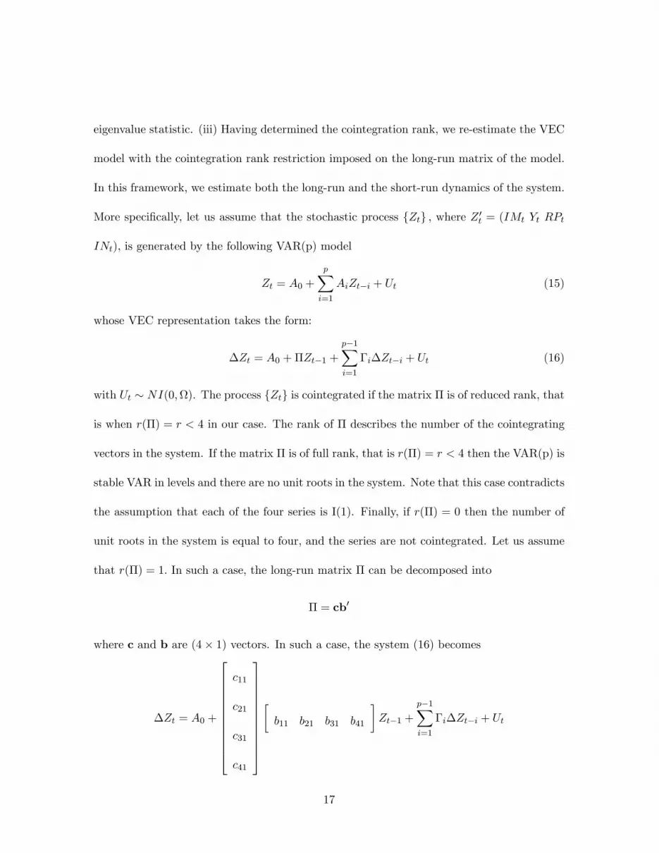
More speci�cally, let us assume that the stochastic process fZtg ; where Z 0t = (IMt Yt RPt
INt); is generated by the following VAR(p) model
Zt = A0 +
pXi=1
AiZt�i + Ut (15)
whose VEC representation takes the form:
�Zt = A0 +�Zt�1 +
p�1Xi=1
�i�Zt�i + Ut (16)
with Ut � NI(0;). The process fZtg is cointegrated if the matrix � is of reduced rank, that
is when r(�) = r < 4 in our case. The rank of � describes the number of the cointegrating
vectors in the system. If the matrix � is of full rank, that is r(�) = r < 4 then the VAR(p) is
stable VAR in levels and there are no unit roots in the system. Note that this case contradicts
the assumption that each of the four series is I(1). Finally, if r(�) = 0 then the number of
unit roots in the system is equal to four, and the series are not cointegrated. Let us assume
that r(�) = 1: In such a case, the long-run matrix � can be decomposed into
� = cb0
where c and b are (4� 1) vectors. In such a case, the system (16) becomes
�Zt = A0 +
266666666664
c11
c21
c31
c41
377777777775�b11 b21 b31 b41
�Zt�1 +
p�1Xi=1
�i�Zt�i + Ut
17

It can be seen that the vector b contains the long-run parameters of the system, whereas the
vector c contains the adjustment coe¢ cients of each of the four variables IMt Yt RPt INt to
the disequilibrium error of the of the previous period.
3.3 Results
We use the Johansen (1988), and Johansen and Juselius (1990) procedure in order to test
for cointegration and to determine the number of long-run relations. We choose the 2 lag
speci�cation for our VAR since the 1 lag speci�cation su¤ers from serial correlation. Our
results are reported in Table 1. We �rst examine whether in the absence of the inequality
variable there is cointegration among real imports, real GDP and relative prices. As can
be seen from column (1), there is no evidence of cointegration among IM; Y and RP . The
inclusion of inequality as an additional determinant of the volume of imports provides us
with evidence of cointegration according to both the trace test and the maximal eigenvalue
statistics - see column (2).17 All reported coe¢ cients (the elements of the cointegration vector
b) are signi�cant. The income elasticity of imports is 1.6, lower than the estimates reported
by Chinn (2005a). The relative price sensitivity is 0.15 and has the expected negative sign.
Inequality has a positive and signi�cant e¤ect on imports.
17 The cointegrating equation reported in Table 1 does not include a time trend. Nevertheless, even if weinclude a time trend in the regressors of column (2), we still get a cointegrating vector according to the tracetest.
18

TABLE 1: Import Cointegration Results I
Long Run US real imports, IM
Coe¢ cients, �i (1) (2) (3)
Cointegr. vectors:
trace test 0 1 1
max. eigenvalue 0 1 1
Y 1:980(0:080)
1:614(0:181)
1:11(0:076)
RP �0:345(0:227)
�0:155(0:046)
IN 1:220(0:189)
3:03(0:289)
REER �0:11(0:04)
constant -11:00 -12:38 -14:05
lag 2 2 1
N 46 46 25
Error correction coe¢ cients
IM �0:638(0:181)
�0:873(0:362)
Y �0:169(0:09)
�0:070(0:125)
RP 0:592(0:22)
IN 0:167(0:06)
�0:075(0:089)
REER �0:602(0:230)
Notes: Standard errors in parentheses.
Column (3) of Table 1 reports estimates using the real exchange rate, REER as an
19

alternative measure of competitiveness. Again, a long run relationship is detected only
after the inclusion of inequality, IN among the determinants of the volume of imports in a
VAR(1) speci�cation. In this case, the income elasticity is close to unity whereas inequality
has an even stronger impact on imports. However, as in Hooper et al (1998), we obtain
an incorrect sign for the real exchange rate elasticity. The error correction coe¢ cients of
real imports reported in the last two columns of Table 1 are negative and signi�cant under
both speci�cations. This indicates that in the presence of disequilibrium the volume of
imports gradually adjusts towards its long-run value. Finally, the residuals of both models
satisfy homoskedasticity, and normality. However, the residuals of model (3) su¤er from
serial correlation.
In order to get an idea for the importance of inequality in shaping the evolution of
US imports, we depict in Figure 3 the �tted values of imports derived from the long run
imports equation shown in column (2) of Table 1 (series 1), whereas series 2 represents the
�tted values of imports which would obtain had inequality remained constant at its 1975
level. Series 3 depicts the actual evolution of US imports. According to our estimates, had
inequality remained at its 1975 level, the �tted value of imports in 1996 would have been
19% lower than the �tted value of imports derived by using the actual level of inequality for
1996. The further rise in inequality since 1996 depicted by more recent but shorter data sets
(see Current Population Survey, U.S. Census Bureau), implies that had inequality in 2004
been at its 1975 level, the percentage decline in US imports in 2004 would have been even
larger than in 1996, thus implying a very large improvement in the current account de�cit.
20

0
100
200
300
400
500
600
700
800
900
1000
1970 1975 1980 1985 1990 1995 2000
US im
ports
Series1
Series2
Series3
Figure 3: US imports
3.4 Robustness
In this section we address the following questions:
(i) How robust are our empirical results to the choice of the cointegration estimation
method? In other words, how di¤erent would our results be if we adopted other asymptoti-
cally e¢ cient cointegration estimators?
(ii) The Johansen cointegration method is asymptotically optimal. However, in samples
as small as ours (46 observations) it has been reported that the Johansen method as well
as other asymptotically equivalent methods su¤er from small sample bias [see Hargreaves,
(1994), Inder (1993) and Gonzalo (1994)]. This bias depends on the dynamics of the system.
For example in the context of the triangular model of cointegration of Phillips (1991) this
bias depends on the Granger causality structure between the cointegration error and the
21

error that drives the regressor and the serial correlation properties of the former.
To address these questions we take the following two steps: First, since our previous
results indicate a single cointegrating vector, we estimate our model with two other asymp-
totically e¢ cient single equation cointegration methods. Second, we perform a small Monte
Carlo experiment to assess the relative performance of the alternative estimators for a sam-
ple equal to that used in the estimation and a Data Generation Process which resembles as
closer as possible the one that is likely to have given rise to the observed data.
3.4.1 Alternative cointegration methods
As far as cointegration estimators are concerned we consider, apart from the Johansen pro-
cedure (JOH) described in the previous section, the following estimators: (i) The simple
OLS which is not asymptotically e¢ cient but is included as a benchmark. (ii) the Autore-
grssive Distributed Lag estimator (ARDL) suggested by Pesaran and Y. Shin (1999) (see
also Phillips and M Loretan (1991) for a version of ARDL) (iii) the semi-parametric Fully
Modi�ed Least Squares (FMLS) estimator of Phillips and Hansen (1990) The di¤erence be-
tween FMLS and ARDL(p,q,k) lies in the way the �long-run correlation�and �endogeneity�
cointegration e¤ects are accounted for. In particular, FMLS generates estimates of the nui-
sance parameters present in the asympotic distribution of OLS non-parametrically, whereas
ARDL eliminates the nuisance parameters from the limiting distributions by estimating a
full dynamic model including lags and leads of the variables in the system (see Pesaran and
Shin (1999), and Panopoulou and Pittis (2004)).
Table 2 presents the results for these alternative cointegration estimators. These results
should be compared with those reported in the second column of Table 1. This comparison
22

reveals that our results are robust across the di¤erent methods: not only all coe¢ cients are
signi�cant and of the same sign independently of the estimation method used, but also the
income and relative price elasticities vary very little across all estimation methods. We also
observe that the inequality elasticity of imports increases from 0.8 to 1.2 when the Johansen
and FMLS are used. However, even under the lower elasticity, the e¤ect of the rise in US
inequality on US imports would still be very large - it would imply that imports in 2004 would
have been lower by about 12% of their 1996 value (25% of their 2004 value) had inequality
remained at its 1975 level.
TABLE 2 : Import Cointegration Results II
US real imports, IM
Method OLS ARDL� FMLS��
Y 1:707(0:02)
1:747(0:046)
1:683(0:019)
RP �0:170(0:045)
�0:252(0:100)
�0:244(0:041)
IN 0:784(0:166)
0:861(0:346)
1:24(0:155)
constant �11:58(0:530)
�12:18(1:123)
�13:04(0:488)
N 49 48 48
Notes: Standard errors in parentheses,
� The Schwartz Order Selection Criterion suggested one lag of IM and one lag of Y: No time
trend is included.
�� Bartlett weights have been used. A truncation lag of 8 has been selected. 8 is the lag that, ac-
cording to the Monte Carlo experiment of the following section, eliminates the bias for this parameters
con�guration.
Still since the rise of the GINI elasticity is realtively large when either the JOH or FMLS
23

procedures are employed, a natural question to ask is which estimate we trust. This question
cannot be answered by appealing to asymptotic arguments, since all the three estimators
(JOH, ARDL, FMLS) are asymptotically equivalent. Therefore, in order to assess the relative
performance of the alternative estimators, we proceed to Monte Carlo simulations. In the
following section we run a small Monte Carlo experiment for a sample equal to that used in
the estimation (49 observations) and a Data Generation Process which resembles as close as
possible the one that is likely to have given rise to the observed data.
3.4.2 A Monte Carlo experiment
We shall assess the performance of these estimators in the context of the triangular model of
cointegration suggested by Phillips (1991). In our case and assuming that the cointegration
error and the errors that drive the regressors follow a VAR(1) model, we have
yt = c+ b>xt + u1t (17)
xt = I3xt�1 + et2664 u1tet
3775 =2664 a11 a>12
a21 A22
37752664 u1t
et�1
3775+2664 �1t�t
3775and 2664 �1t
�t
3775 � NIID2664 0
0
3775 ;2664 �11 �>12
�12 �22
3775 (18)
where xt = [x1t; x2t; x3t]>; b = [b1; b2; b3]
>; et = [e1t; e2t; e3t]>; �t = [�1t; v2t; v3t]
>: In the
context of our empirical model, yt denotes real imports, IM , x1 denotes real GDP, Y , x2
denotes relative prices, RP and x3 denotes inequality, IN .
24

One can make the following remarks regarding the estimators used in our analysis as
opposed to the OLS estimator:
(i) The presence of nuisance parameters (cointegration e¤ects) in the asymptotic dis-
tribution of the OLS estimator can be due to either (a) Granger causality from et to u1t
(a12 6= 0); and/or (b) Granger causality from u1t to et ( a21 6= 0); and/or (c) contempora-
neous correlation between et and u1t ( �12 6= 0): In other words, if a12; a21 and �12 were all
zero vectors then the OLS estimator would be the optimal estimator for estimating b.18
(ii) The asymptotically e¢ cient estimators, namely JOH, ARDL and FMLS basically
deal with the nuisance parameters of the OLS estimator asymptotically. However, in the
presence of a small sample some remaining e¤ects may be manifested in biases produced
even by JOH, ARDL and FMLS.
(iii) The previous remarks suggest that di¤erent estimates among JOH, ARDL and FMLS
may arise depending on the relative ability of each estimator to remove the cointegration
e¤ects �relatively fast�. Moreover, if these e¤ects were present only in speci�c location of
the above system, then these estimators would di¤er only with respect to the corresponding
parameter. For example, if only e3t were either temporally or contemporaneously correlated
with u1t then the estimators are likely to produce di¤erent estimates of only say b3:
Next, we callibrate the above model using our data. This gives us estimates of a11;
a12;a21; A22; �11;�12;�22: These estimates allow us to simplify our Monte Carlo design, by
moving to a lower dimensional model where we have only one regressor. This is due to the
fact that our estimates suggest Granger causality and (negative) contemporaneous correlation
18 Some further corrections would be necessary for estimating its standard error if a11 6= 0:
25

mainly between u1t and e3t: As a result, we adopt the following DGP:
yt = �xt + u1t (19)
with � = 1,
xt = xt�1 + et
0BB@ u1t
et
1CCA =
0BB@ 0:7 �0:21
0:30 0:30
1CCA0BB@ u1t�1
et�1
1CCA+0BB@ �1t
�2t
1CCA (20)
and
0BB@ �1t
�2t
1CCA ~NIID26640BB@ 0
0
1CCA0BB@ 0:0014 �0:00019
�0:00019 0:00031
1CCA3775 (21)
Regarding the assesment of our estimators, all estimators of � are compared on the basis of
the following three statistics:
1) Bias, computed as:
b� � �0where:
b� = rXi=1
b�i=ri = 1; :::; r and r is the number of replications and �0 = 1.
2) Average standard error, astde(b�)astde(b�) =
vuut rXi=1
�b�i � ��2 =r3) Average root mean squared error, rmse(b�), computed according to the previous formula
in which � has been replaced by �0:
26

TABLE 3 : Monte Carlo Results
Mean bias Standard error Root mean sq. error
Panel A: Sample size= 49
Estimator
OLS �0:0995 0:2035 0:0513
ARDL �0:0318 0:2266 0:0523
JOHANSEN �0:0115 0:2157 0:0466
FMLS �0:0232 0:1038 0:0113
Panel B: Sample size:=490
Estimator
OLS �0:0090 0:0200 0:0005
ARDL �0:0004 0:0187 0:0003
JOHANSEN �0:0015 0:0131 0:0002
FMLS �0:0022 0:0124 0:0002
Panel C: Sample size=4900
Estimator
OLS �0:0010 0:0020 0:000
ARDL �0:0001 0:0018 0:000
JOHANSEN �0:0002 0:0013 0:000
FMLS �0:0002 0:0013 0:000
Number of replications: 1000
The results of 1000 replications of the above model are presented in Table 3. Panel
27

A reports simulations results for a sample size of 49 observations. As expected, the OLS
appears to be the worst estimator of all, since it exhibits the largest bias and variation. On
the other hand, the Johansen speci�cations consistently outperforms the ARDL procedure
in terms of the bias, the standard deviation and root mean square error. However, the fully
modi�ed estimator outperforms the ARDL dynamic speci�cation in terms of variation. JOH
and FMLS exhibit the lowest bias and variation of all estimators, which implies that it is
more likely to be closer to the true value with these two estimators than with any other
estimator. In terms of mean bias, the ARDL procedure fairs well in comparison to the
simple OLS, but appears to be about three times worse than the Johansen procedure. Thus
our results strongly support the superiority of the fully modi�ed estimator and the Johansen
estimator for estimation and inference on �. These procedures appear to be the best since
they minimize the corresponding biases and the variation. Note that these procedures also
imply the highest inequality elasticity of imports.
Finally, we investigate the e¤ect of the sample size on the estimators�performance. Panel
B and C report the Monte Carlo results when our sample increases by a factor of 10 in
panel B and by a factor of 100 in panel C. As expected, the bias becomes negligible for
all the estimators as our sample increases, with only the OLS bias remaining relatively
high (OLS does not account for the cointegration e¤ects even asymptotically, although it is
super consistent). Moreover, the standard deviation (and the root mean squared error) is
almost the same for all estimators. These results are consistent with the relevant asymptotic
theory. Indeed, our results show that the bias for all estimators decrease at a rate close to T
(instead ofpT ). For example, the bias of the OLS and FMLS at T=1 is -0.0995 and -0.0232
28

respectively, whereas at T=10 the bias decreases to -0.0090 and -0.0022 respectively and at
T=100 the bias decreases further to -0.001 and -0.0002 respectively.
4 Concluding Remarks
The present paper explains our �nding that US income inequality has a signi�cant in�uence
on the US demand for imports on the basis of a model in which trade is conducted in
vertically-di¤erentiated products. However, one could advance alternative explanations for
this �nding. For example, if one assumes that preferences are non-homothetic, and imports
have a higher income elasticity than domestically produced goods, then changes in inequality
can a¤ect the demand for imports even if trade is conducted in homogeneous goods. Given
our objective to improve on the standard speci�cations of the aggregate import demand
function we regard the existence of alternative channels for the in�uence of inequality on
the demand for imports as a plus; after all, despite the increasing importance of vertically-
di¤erentiated products in world trade, the share of international trade that is conducted in
either homogeneous goods or in horizontally-di¤erentiated products remains signi�cant.
In this paper, in line with Rose and Yellen (1989), Meade (1992), Johnston and Chinn
(1996) and Chinn (2005b), we �nd no evidence for the existence of a long run relationship
between agrregate imports, income and competitiveness in the US. However, the addition of
US income inequality as a determinant of the aggregate demand for imports improves the
picture signi�cantly. Using US data for the 1948-1996 period we �nd not only that there is a
stable long run relationship between aggregate imports, income relative prices and inequality,
but that the in�uence of inequality is quantitatively very important as well. This result
appears robust accross alternative methods of estimating cointegration equations. Moreover,
29

Monte Carlo simulations suggest that the methods delivering the highest inequality impact
on imports are those with the best performance in small samples.
References
Acemoglu, D. (2002), "Technical Change, Inequality and the Labor Market", Journalof Economic Literature, 40, 1, pp. 7-72.
Armington, P.S. (1969), �A theory of demand for products distinguished by place oflocation�, IMF Sta¤ Papers, 26, pp. 159-178.
Boyd D., G.M. Caporale and R. Smith (2001), "Real Exchange Rate E¤ects on theBalance of Trade: Cointegratiopn and the Marshall-Lerner Condition", InternationalJournal of Finance and Economics, 6, pp. 187-200
Bowen, H.P., E. Leamer, and L. Sviekauskas (1987), �Multicountry, Multifactor Testsof the Factor Abundance Theory", American Economic Review, 82, pp. 371-392.
Brandolini A. (1998 ), "A Bird�s-Eye View of Long-Run Changes in Income Inequality",Banca d�Italia Research Department.
Chinn, M. (2005a), "Doomed to De�cits? Aggregate U.S. Trade Flows Re-Examined",Review of World Economics, 141(3), pp. 460-485.
Chinn, M. (2005b), "Incomes, Exchange Rates and the U.S. trade De�cit, Once Again",International Finance, 7(3), pp. 1-19.
Creedy, J. (1977), �Pareto and the Distribution of Income,� Review of Income andWealth, 23, pp. 405-411.
Deininger, A. and L. Squire (1996), A new data set measuring inequality, WIDER,Word Bank.
Flam, H. and E. Helpman (1987), "Vertical Product Di¤erentiation and North-SouthTrade", American Economic Review, 77, pp. 810-822.
Francois, J.and S. Kaplan (1996), �Aggregate Demand Shifts, Income Distribution,and the Linder Hypothesis.�Review of Economics and Statistics, 78, 2 , pp. 244-250.
Goldstein, M. and M.S. Khan (1985), �Income and Price E¤ects in Foreign Trade�,in R. W. Jones and P.B.Kenen (eds), Handbook of International Economics, Vol. 2,North-Holland, New York.
Gonzalo, J. (1994), �Five Alternative Methods of Estimating Long-Run EquilibriumRelationships�, Journal of Econometrics, 60, 203-233.
30

Grossman, G. (1982), " Import competition from developed and developing countries",Review of Economics and Statistics, 64, pp. 271�281.
Hansen, B. (2000), "Sample Splitting and Threshold Estimation", Econometrica, 68,pp.575-603.
Hargreaves, C.P. (1994), �A Review of Methods of Estimating Cointegrating Relation-ships�in C.P. Hargreaves (ed.), Nonstationary Time Series Analysis and Cointegration,87-132, Oxford University Press, Oxford.
Helkie, W. and P. Hooper (1988), "An Empirical Analysis of the External De�cit,1980-86", in R. Bryant, G. Holtham and P. Hooper, External De�cits and the Dollar,Brookings Institution.
Hooper, P., and J. Marquez (1995), "Exchange rates, prices, and external adjustmentin the United States and Japan", in Kenen, P. (ed.), Understanding Interdependence,Princeton University Press, Princeton, NJ.
Hooper, P, Johnson K. and J. Marquez (1998), "Trade Elasticities for G-7 Countries",International Finance Discussion Papers No. 609, Federal Reserve Board, WashingtonD.C.
Houthakker, H., and S. Magee (1969), "Income and price elasticities in world trade",Review of Economics and Statistics, 51, pp.111�125.
Hunter, L. (1991), �The Contribution of Nonhomothetic Preferences to Trade�, Journalof International Economics 30, pp. 345-358.
Inder, B. (1993), �Estimating Long-Run Relationships in Economics. A Comparison ofDi¤erent Approaches�, Journal of Econometrics, 57, pp. 53-68.
Johansen, S. (1988), "Statistcal Analysis of Cointegration Vectors", Journal of Eco-nomic Dynamics and Control 12, pp. 231-254.
Johansen, S. and K. Juselius (1990), "Maximum Likelihood Estimation and Inferenceon Cointegration with Application to the Demand for Money", Oxford Bulletin ofEconomics and Statistics 52, pp. 169-210.
Johansen, Soren, 1991. "Estimation and Hypothesis Testing of Cointegration Vectorsin Gaussian Vector Autoregressive Models," Econometrica, 59, pp 1551-80.
Johnston, L.D. and M. Chinn (1996), "How well is America Competing? A Commenton Papadakis", Journal of Policy Analysis and Management 15(1), pp. 68-81.
Katsimi, M. and T. Moutos (2005), "Inequality and Relative Reliance on Tari¤s: The-ory and Evidence", CESifo Working Paper No. 1457.
Kohli, U.R. (1982), �Relative price e¤ects and the demand for imports�, CanadianJournal of Economics, 15, pp. 205-219.
31

Krugman, P. (1989), "Di¤erences in Income Elasticities and Trends in Real ExchangeRates", European Economic Review, 33, pp. 1031-1054.
Linder, S. (1961), An Essay on Trade and Transformation, Almqvist and Wiksells,Uppsala.
Malley, J.and T. Moutos, (2002), "Vertical product di¤erentiation and the importdemand function: theory and evidence", Canadian Journal of Economics, 35, pp. 257-281.
Marquez, J. (2000), "The Puzzling Income Elasticity of US Imports", World Conferenceof Econometric Society.
Marquez, J. (2002), Estimating Trade Elasticities, Kluwer Academic Publishers,Boston.
Meade, E. (1991), "A Fresh Look at the Resposiveness of Trade Flows to ExchangeRates", Annual meeting of the Western Economic Association.
Mitra, D. and V. Trindade (2003), �Inequality and Trade.�NBER Working Paper No.10087.
Markusen, J. (1986), �Explaining the Volume of Trade: an Eclectic Approach�, Amer-ican Economic Review, 76, 5, pp.1002-1011.
Panopoulou, E. and N. Pittis (2004), "A Comparison of Autoregressive DistributedLag and Dynamic OLS Cointegration Estimators in the Case of a Serially CorrelatedCointegration Error", Econometrics Journal, 7, pp. 585-687.
Pesaran, M.H. and Y. Shin (1999) "An Autoregressive Distributed Lag Modelling Ap-proach to Cointegration Analysis", in S. Strom (ed.) Econometrics and Economic The-ory in the 20th Century: The Ragnar Frish Centennial Symposium, Econometric So-ciety Monograph, Cambridge University Press, Cambridge.
Phillips, P.C.B. and B.E. Hansen (1990) "Statistical Inference in Instumental VariablesRegression withI(1) Processes,"Review of Economic Studies, 57:99-125.
Phillips, P.C.B. (1991) "Optimal Inference in Cointegrated Systems,�Econometrica,59, pp. 283-306.
Phillips, P.C.B. and M. Loretan (1991), "Estimating Long-run Economic Equilibria",Review of Economic Studies, 58, pp. 407-436.
Rose, A. (1991), "The Role of Exchange Rates in a Popular Model of InternationalTrade: Does the �Marshall-Lerner� Condition Hold?� Journal of International Eco-nomics, 30, pp. 301-316.
Rose, A. and J. Yellen (1989), "Is there a J-Curve?", Journal of Monetary Economics,24, pp. 53-68.
32

Rosen, S. (1974), "Hedonic Prices and Implicit Markets: Product Di¤erentiation inPure Competition", Journal of Political Economy, 82, pp. 34-55.
Schott, P. (2003), "Across-Product versus Within-Product Specialization in Interna-tional Trade", Quarterly Journal of Economics, 108, pp. 657-691.
Tre�er, D. (1995), �The Case of the Missing Trade and Other Mysteries,�AmericanEconomic Review, 85, pp.1029-1046.
33

CESifo Working Paper Series (for full list see Twww.cesifo-group.de)T
___________________________________________________________________________ 1764 Didier Laussel and Raymond Riezman, Fixed Transport Costs and International Trade,
July 2006 1765 Rafael Lalive, How do Extended Benefits Affect Unemployment Duration? A
Regression Discontinuity Approach, July 2006 1766 Eric Hillebrand, Gunther Schnabl and Yasemin Ulu, Japanese Foreign Exchange
Intervention and the Yen/Dollar Exchange Rate: A Simultaneous Equations Approach Using Realized Volatility, July 2006
1767 Carsten Hefeker, EMU Enlargement, Policy Uncertainty and Economic Reforms, July
2006 1768 Giovanni Facchini and Anna Maria Mayda, Individual Attitudes towards Immigrants:
Welfare-State Determinants across Countries, July 2006 1769 Maarten Bosker and Harry Garretsen, Geography Rules Too! Economic Development
and the Geography of Institutions, July 2006 1770 M. Hashem Pesaran and Allan Timmermann, Testing Dependence among Serially
Correlated Multi-category Variables, July 2006 1771 Juergen von Hagen and Haiping Zhang, Financial Liberalization in a Small Open
Economy, August 2006 1772 Alessandro Cigno, Is there a Social Security Tax Wedge?, August 2006 1773 Peter Egger, Simon Loretz, Michael Pfaffermayr and Hannes Winner, Corporate
Taxation and Multinational Activity, August 2006 1774 Jeremy S.S. Edwards, Wolfgang Eggert and Alfons J. Weichenrieder, The Measurement
of Firm Ownership and its Effect on Managerial Pay, August 2006 1775 Scott Alan Carson and Thomas N. Maloney, Living Standards in Black and White:
Evidence from the Heights of Ohio Prison Inmates, 1829 – 1913, August 2006 1776 Richard Schmidtke, Two-Sided Markets with Pecuniary and Participation Externalities,
August 2006 1777 Ben J. Heijdra and Jenny E. Ligthart, The Transitional Dynamics of Fiscal Policy in
Small Open Economies, August 2006 1778 Jay Pil Choi, How Reasonable is the ‘Reasonable’ Royalty Rate? Damage Rules and
Probabilistic Intellectual Property Rights, August 2006

1779 Ludger Woessmann, Efficiency and Equity of European Education and Training
Policies, August 2006 1780 Gregory Ponthiere, Growth, Longevity and Public Policy, August 2006 1781 Laszlo Goerke, Corporate and Personal Income Tax Declarations, August 2006 1782 Florian Englmaier, Pablo Guillén, Loreto Llorente, Sander Onderstal and Rupert
Sausgruber, The Chopstick Auction: A Study of the Exposure Problem in Multi-Unit Auctions, August 2006
1783 Adam S. Posen and Daniel Popov Gould, Has EMU had any Impact on the Degree of
Wage Restraint?, August 2006 1784 Paolo M. Panteghini, A Simple Explanation for the Unfavorable Tax Treatment of
Investment Costs, August 2006 1785 Alan J. Auerbach, Why have Corporate Tax Revenues Declined? Another Look, August
2006 1786 Hideshi Itoh and Hodaka Morita, Formal Contracts, Relational Contracts, and the
Holdup Problem, August 2006 1787 Rafael Lalive and Alejandra Cattaneo, Social Interactions and Schooling Decisions,
August 2006 1788 George Kapetanios, M. Hashem Pesaran and Takashi Yamagata, Panels with
Nonstationary Multifactor Error Structures, August 2006 1789 Torben M. Andersen, Increasing Longevity and Social Security Reforms, August 2006 1790 John Whalley, Recent Regional Agreements: Why so many, why so much Variance in
Form, why Coming so fast, and where are they Headed?, August 2006 1791 Sebastian G. Kessing and Kai A. Konrad, Time Consistency and Bureaucratic Budget
Competition, August 2006 1792 Bertil Holmlund, Qian Liu and Oskar Nordström Skans, Mind the Gap? Estimating the
Effects of Postponing Higher Education, August 2006 1793 Peter Birch Sørensen, Can Capital Income Taxes Survive? And Should They?, August
2006 1794 Michael Kosfeld, Akira Okada and Arno Riedl, Institution Formation in Public Goods
Games, September 2006 1795 Marcel Gérard, Reforming the Taxation of Multijurisdictional Enterprises in Europe, a
Tentative Appraisal, September 2006

1796 Louis Eeckhoudt, Béatrice Rey and Harris Schlesinger, A Good Sign for Multivariate
Risk Taking, September 2006 1797 Dominique M. Gross and Nicolas Schmitt, Why do Low- and High-Skill Workers
Migrate? Flow Evidence from France, September 2006 1798 Dan Bernhardt, Stefan Krasa and Mattias Polborn, Political Polarization and the
Electoral Effects of Media Bias, September 2006 1799 Pierre Pestieau and Motohiro Sato, Estate Taxation with Both Accidental and Planned
Bequests, September 2006 1800 Øystein Foros and Hans Jarle Kind, Do Slotting Allowances Harm Retail Competition?,
September 2006 1801 Tobias Lindhe and Jan Södersten, The Equity Trap, the Cost of Capital and the Firm’s
Growth Path, September 2006 1802 Wolfgang Buchholz, Richard Cornes and Wolfgang Peters, Existence, Uniqueness and
Some Comparative Statics for Ratio- and Lindahl Equilibria: New Wine in Old Bottles, September 2006
1803 Jan Schnellenbach, Lars P. Feld and Christoph Schaltegger, The Impact of Referendums
on the Centralisation of Public Goods Provision: A Political Economy Approach, September 2006
1804 David-Jan Jansen and Jakob de Haan, Does ECB Communication Help in Predicting its
Interest Rate Decisions?, September 2006 1805 Jerome L. Stein, United States Current Account Deficits: A Stochastic Optimal Control
Analysis, September 2006 1806 Friedrich Schneider, Shadow Economies and Corruption all over the World: What do
we really Know?, September 2006 1807 Joerg Lingens and Klaus Waelde, Pareto-Improving Unemployment Policies,
September 2006 1808 Axel Dreher, Jan-Egbert Sturm and James Raymond Vreeland, Does Membership on
the UN Security Council Influence IMF Decisions? Evidence from Panel Data, September 2006
1809 Prabir De, Regional Trade in Northeast Asia: Why do Trade Costs Matter?, September
2006 1810 Antonis Adam and Thomas Moutos, A Politico-Economic Analysis of Minimum Wages
and Wage Subsidies, September 2006 1811 Guglielmo Maria Caporale and Christoph Hanck, Cointegration Tests of PPP: Do they
also Exhibit Erratic Behaviour?, September 2006

1812 Robert S. Chirinko and Hisham Foad, Noise vs. News in Equity Returns, September
2006 1813 Oliver Huelsewig, Eric Mayer and Timo Wollmershaeuser, Bank Behavior and the Cost
Channel of Monetary Transmission, September 2006 1814 Michael S. Michael, Are Migration Policies that Induce Skilled (Unskilled) Migration
Beneficial (Harmful) for the Host Country?, September 2006 1815 Eytan Sheshinski, Optimum Commodity Taxation in Pooling Equilibria, October 2006 1816 Gottfried Haber and Reinhard Neck, Sustainability of Austrian Public Debt: A Political
Economy Perspective, October 2006 1817 Thiess Buettner, Michael Overesch, Ulrich Schreiber and Georg Wamser, The Impact of
Thin-Capitalization Rules on Multinationals’ Financing and Investment Decisions, October 2006
1818 Eric O’N. Fisher and Sharon L. May, Relativity in Trade Theory: Towards a Solution to
the Mystery of Missing Trade, October 2006 1819 Junichi Minagawa and Thorsten Upmann, Labor Supply and the Demand for Child
Care: An Intertemporal Approach, October 2006 1820 Jan K. Brueckner and Raquel Girvin, Airport Noise Regulation, Airline Service Quality,
and Social Welfare, October 2006 1821 Sijbren Cnossen, Alcohol Taxation and Regulation in the European Union, October
2006 1822 Frederick van der Ploeg, Sustainable Social Spending in a Greying Economy with
Stagnant Public Services: Baumol’s Cost Disease Revisited, October 2006 1823 Steven Brakman, Harry Garretsen and Charles van Marrewijk, Cross-Border Mergers &
Acquisitions: The Facts as a Guide for International Economics, October 2006 1824 J. Atsu Amegashie, A Psychological Game with Interdependent Preference Types,
October 2006 1825 Kurt R. Brekke, Ingrid Koenigbauer and Odd Rune Straume, Reference Pricing of
Pharmaceuticals, October 2006 1826 Sean Holly, M. Hashem Pesaran and Takashi Yamagata, A Spatio-Temporal Model of
House Prices in the US, October 2006 1827 Margarita Katsimi and Thomas Moutos, Inequality and the US Import Demand
Function, October 2006